For $Y\gg\ln x\sim\ln(1-x)$, $N(Y+\ln x)$ ($N(Y+\ln(1-x))$) can be replaced by $N(Y)$ in the hard partonic splitting region $x\sim 1$ ($1-x\sim 1$) (non-singular or regular parts of the splitting functions), while the dependence on $\ln x$ is kept on the singular one $\Phi(x)\approx N_{s}/x$ as it is performed in the vacuum. Furthermore, the integration over $x$ can be replaced by the integration over $Y(x)=\ln\left(\frac{xE\Theta}{Q_{0}}\right)$

$$\int^{1}\gamma_{0}^{2}(x)\frac{dx}{x}=\int^{Y}\gamma_{0}^{2}(Y(x))dY(x).$$

(7)

After applying the differential operator $\frac{d}{dY}$ to both members of the system (3,4) above, one is left with the approximate system of coupled equations,

	$\displaystyle\frac{d^{2}}{dY^{2}}N_{g}(Y)\!\!$	$\displaystyle\!\!=\!\!$	$\displaystyle\!\!\gamma_{0}^{2}\left(N_{s}-a_{1}\frac{d}{dY}\right)N_{g}(Y),$		(8)
	$\displaystyle\frac{d^{2}}{dY^{2}}N_{q}(Y)\!\!$	$\displaystyle\!\!=\!\!$	$\displaystyle\!\!\frac{C_{F}}{N_{c}}\gamma_{0}^{2}\left(N_{s}-\tilde{a}_{1}\frac{d}{dY}\right)N_{g}(Y),$		(9)

with the initial conditions at threshold $N_{A}^{h}(0)=1$ and $N_{A}^{{}^{\prime}h}(0)=0$ and the hard constants

$$a_{1}=\frac{1}{4N_{c}}\left[\frac{11}{3}N_{c}+\frac{4}{3}T_{R}\left(1-2\frac{C_{F}}{N_{c}}\right)\right],\qquad\tilde{a}_{1}=\frac{3}{4}.$$

The quantum corrections $\propto a_{1},\;\tilde{a}_{1}$ in (8,9) arise from the integration over the regular part of the splitting functions, they are ${\cal O}(\sqrt{\alpha}_{s})$ suppressed and partially account for energy conservation as happens in the absence of the dense medium. Since only the DLA terms are medium-enhanced in (8,9), the hard constants are $N_{s}$-independent.

These equations can be solved by applying the inverse Mellin transform:

$$N_{g}(Y)=\int_{C}\frac{d\omega}{2\pi i}e^{\omega Y^{\prime}}N_{g}(\omega)$$

(10)

to the self-contained gluonic equation (8), where the contour $C$ lies to the right of all singularities of $N_{G}(\omega)$ in the complex plane. The running of the coupling constant $\alpha_{s}(Y)$, Eq. (2), is taken into account through the identity

$$\int_{C}\frac{d\omega}{2\pi i}Y^{\prime}e^{\omega Y^{\prime}}N_{g}(\omega)=-\int_{C}\frac{d\omega}{2\pi i}e^{\omega Y^{\prime}}\left(2\omega N_{g}(\omega)+\omega^{2}\frac{d}{d\omega}N_{g}(\omega)\right).$$

Consequently, one is left with the following differential equation in Mellin space

$$\frac{1}{N_{g}}\frac{d}{d\omega}N_{g}(\omega)=-\frac{N_{s}}{\beta_{0}\omega^{2}}+\left(\frac{a_{1}}{\beta_{0}}-2\right)\frac{1}{\omega}.$$

(11)

Solving (11) and using (10), one obtains

$$N_{g}(Y)\simeq\int_{C}\frac{d\omega}{2\pi i}\omega^{\frac{a_{1}}{\beta_{0}}-2}\exp{\left(\omega Y^{\prime}+\frac{N_{s}}{\beta_{0}\omega}\right)}.$$

(12)

The exact solution of (12) together with the initial conditions leads to a linear combination of two kinds of Bessel functions which resums the perturbative series at all powers of $\sqrt{\alpha}_{s}$ [1]. However, in this paper we are concerned with the asymptotic solution of the equation as $Y\gg 1$ ($E\Theta\gg Q_{0}$), that is the high energy limit. Therefore, the Mellin transform (12) can be estimated by the steepest descent method. Indeed, the large parameter is $Y^{\prime}$ and the function in the exponent presents a saddle point at $\omega_{0}=\sqrt{N_{s}/(\beta_{0}Y^{\prime})}$, such that the asymptotic solution reads

$$N_{g}^{h}(Y)\simeq{\cal K}\times{Y^{\prime}}^{-\frac{\sigma_{1}}{\beta_{0}}}\exp{\sqrt{\frac{4N_{s}}{\beta_{0}}Y^{\prime}}},$$

(13)

where

$$\sigma_{1}=\frac{a_{1}}{2}-\frac{\beta_{0}}{4}.$$

We also introduced, as stressed in the introduction, the LPHD normalization constant ${\cal K}$ [23], which accounts for hadronization effects outside the medium. The constant $\sigma_{1}$ is $N_{s}$-independent because it resums vacuum corrections. Therefore, the production of soft gluons in a dense medium becomes $\exp\left[2(\sqrt{N_{s}}-1)\sqrt{Y^{\prime}/\beta_{0}}\right]$ higher than the standard production of soft gluons in the vacuum [1] and the factor $\sqrt{N_{s}}$ in (13) underlines the presence of the nuclear medium; this results has first been reported in [24]. From (13) one obtains the first and second logarithmic derivatives of $N_{g}$:

$$\frac{1}{N_{g}}\frac{dN_{g}}{dY}\equiv\frac{1}{N_{q}}\frac{dN_{q}}{dY}=\sqrt{N_{s}}\gamma_{0}-\sigma_{1}\gamma_{0}^{2},\quad\frac{1}{N_{g}}\frac{d^{2}N_{g}}{dY^{2}}\equiv\frac{1}{N_{q}}\frac{d^{2}N_{q}}{dY^{2}}=N_{s}\gamma_{0}^{2}.$$

(14)

The expression on the left hand side of (14) is nothing but the MLLA rate of multiparticle production with respect to the evolution-time variable $Y\simeq\ln(\Theta)$ in the medium, which we define as the medium-modified MLLA anomalous dimension:

$$\gamma_{\text{med}}(Y)\equiv\frac{1}{N_{g}}\frac{dN_{g}}{dY}=\sqrt{N_{s}}\gamma_{0}\left[1-\sigma_{1}\frac{\gamma_{0}}{\sqrt{N_{s}}}+{\cal O}\left(\frac{\gamma_{0}^{2}}{N_{s}}\right)\right],$$

(15)

where $N_{s}$ only affects, as expected, the leading double logarithmic term. From (13) and (15), one recovers the ansatz

$$N_{g}(Y)\simeq\exp{\left(\int\gamma_{\text{med}}(Y)dY\right)},$$

(16)

which we further improve in the next paragraph by adding higher order corrections. Finally, using (13) and (8,9), one obtains the solution for $N_{Q}^{h}$:

$$N_{q}(Y)=\frac{C_{F}}{N_{c}}\left[1+\left(a_{1}-\tilde{a}_{1}\right)\frac{\gamma_{0}}{\sqrt{N_{s}}}\right]N_{g}(Y)+{\cal O}\left(\frac{\gamma_{0}^{2}}{N_{s}}\right).$$

(17)

Therefore, we can introduce the medium-modified MLLA gluon to quark average multiplicity ratio $r=N_{g}/N_{q}=N_{g}^{h}/N_{q}^{h}$ in the form

$$r=r_{0}\left[1-r_{1}\frac{\gamma_{0}}{\sqrt{N_{s}}}+{\cal O}\left(\frac{\gamma_{0}^{2}}{N_{s}}\right)\right],\qquad r_{0}=\frac{N_{c}}{C_{F}},\qquad r_{1}=a_{1}-\tilde{a}_{1},$$

(18)

where the suppression factor $1/\sqrt{N_{s}}$ restricts the production of hard collinear partons as $N_{s}>1$. We notice that (18) is identical to the expression with fixed coupling constant $\alpha_{s}(Y)$, where $Y=\ln\left(Q/Q_{0}\right)$ and $Q=E\Theta$ is the virtuality of the jet produced in the nucleus-nucleus reaction. This factor is found to suppress the hard correction ${\cal O}(\gamma_{0})$ and therefore, $r$ approaches its asymptotic DLA limit $r_{0}=N_{c}/C_{F}$ when the coherent radiation of soft gluons is enhanced. Setting $N_{s}=1$ in (18), one recovers the appropriate limits in the vacuum [1, 11, 25]. The constants entering in (13) and (18) are the same as those obtained in the vacuum and their values are displayed in Table 1.

Previous MLLA results for the average multiplicities can be improved by further pushing the perturbative series in (3,4). We can include NNLO or NMLLA corrections of order ${\cal O}(\alpha_{s})$, which are known to better account for energy conservation in the vacuum [12, 17, 20]. For this purpose, we replace $N(Y+\ln x)$ ($N(Y+\ln(1-x)$) by the Taylor expansion $N(Y)+\frac{d}{dY}N(Y)\ln x+\ldots$ ($N(Y)+\frac{d}{dY}N(Y)\ln(1-x)+\ldots$) and, as in section 2.1, we integrate over the non-singular parts of the splitting functions. We thus obtain the medium-modified NMLLA approximate system of two-coupled evolution equations

	$\displaystyle\frac{d^{2}}{dY^{2}}N_{g}(Y)\!$	$\displaystyle\!=\!$	$\displaystyle\!\gamma_{0}^{2}\left(N_{s}-a_{1}\left(\frac{d}{dY}-\beta\gamma_{0}^{2}\right)+a_{2}(N_{s})\frac{d^{2}}{dY^{2}}\right)N_{g}(Y),$		(19)
	$\displaystyle\frac{d^{2}}{dY^{2}}N_{q}(Y)\!$	$\displaystyle\!=\!$	$\displaystyle\!\frac{C_{F}}{N_{c}}\gamma_{0}^{2}\left(N_{s}-\tilde{a}_{1}\left(\frac{d}{dY}-\beta\gamma_{0}^{2}\right)+\tilde{a}_{2}(N_{s})\frac{d^{2}}{dY^{2}}\right)N_{g}(Y),$		(20)

with the new $N_{s}$-dependent constants

$$a_{2}(N_{s})=\frac{67}{36}-N_{s}\frac{\pi^{2}}{6}-\frac{13}{18}\frac{T_{R}}{N_{c}}\frac{C_{F}}{N_{c}}+\frac{2}{3}\frac{T_{R}}{N_{c}}\frac{C_{F}}{N_{c}}\frac{(a_{1}-\tilde{a}_{1})}{\sqrt{N_{s}}},\quad\tilde{a}_{2}(N_{s})=\frac{7}{8}+\frac{C_{F}}{N_{c}}\left(\frac{5}{8}-N_{s}\frac{\pi^{2}}{6}\right).$$

The dependence of $a_{2}$ and $\tilde{a}_{2}$ on $N_{s}$ follows from the singular term in the integral $N_{s}\int_{0}^{1}\frac{dx}{x}\ln(1-x)=-N_{s}\frac{\pi^{2}}{6}$ which also enhances (see below) the induced soft gluon radiation at the NNLO level. The term $\propto 1/\sqrt{N_{s}}$ in $a_{2}(N_{s})$ was obtained by replacing (17) in the single logarithmic piece $\propto N_{q}$ in (3), while the term $\propto N_{s}$ in the equations (19,20) enhances the role of the leading DLA as in (8,9). As expected, one recovers the constants $a_{2}(N_{s}=1)=a_{2}$ and $\tilde{a}_{2}(N_{s}=1)=\tilde{a}_{2}$ obtained in the vacuum [20] when $N_{s}=1$. The terms proportional to these constants are known to better account for energy conservation in the partonic shower in the vacuum. Also note that the contributions $\propto a_{1}\beta_{0}$ and $\tilde{a}_{1}\beta_{0}$ cannot be neglected when performing predictions with running coupling coupling constant.

The system (19,20) can be solved by inserting the ansatz (16) in both sides of (19) with

$$\gamma_{\text{med}}(Y)=\sqrt{N_{s}}\gamma_{0}\left[1-\sigma_{1}\frac{\gamma_{0}}{\sqrt{N_{s}}}-\sigma_{2}(N_{s})\frac{\gamma_{0}^{2}}{N_{s}}+{\cal O}\left(\frac{\gamma_{0}^{3}}{N_{s}^{3/2}}\right)\right],$$

(21)

where $\sigma_{2}(N_{s})$ is the unknown coefficient to be determined. The medium-modified NMLLA anomalous dimension (21) has been inspired from the MLLA (15) where, in both cases, we make appear the rescaling of the coupling constant $\alpha_{s}\to\alpha_{s}/N_{s}$ in the series. After equating terms $\propto\gamma_{0}^{2}$ in the left and right hand sides of (19) we obtain the following value

$$\sigma_{2}(N_{s})=-\frac{1}{2}\left(\frac{1}{2}a_{1}\beta_{0}+\frac{1}{4}a_{1}^{2}+N_{s}a_{2}(N_{s})+\frac{3}{16}\beta_{0}^{2}\right),$$

(22)

such that after integrating (21) according to (16), the medium-modified NMLLA average multiplicity takes the simple form

$\displaystyle N_{g}^{h}(Y)\simeq{\cal K}\times{Y^{\prime}}^{-\frac{\sigma_{1}}{\beta_{0}}}\exp\left[{\sqrt{\frac{4N_{s}}{\beta_{0}}Y^{\prime}}}+\frac{2\sigma_{2}(N_{s})}{\sqrt{N_{s}\beta^{3}_{0}Y^{\prime}}}\right].$

(23)

The term $\propto\sigma_{2}(N_{s})$ in (23) provides the NMLLA correction to $N_{G}^{h}$. As $N_{s}$ increases, $\sigma_{2}(N_{s})$ follows the leading behavior $\sigma_{2}(N_{s})\simeq N_{s}^{2}$ (and the second factor in the exponent of (23) $\simeq N_{s}^{3/2}$) which enhances the production of induced soft gluons in the medium at the NNLO level. Setting $N_{s}=1$ in (23) one recovers the value of this constant in the vacuum $\sigma_{2}(N_{s}=1)\stackrel{{\scriptstyle n_{f}=3}}{{=}}-0.378$ as given in [12]. Furthermore, setting $\beta_{0}=0$ in (22), the appropriate limit with fixed coupling constant $\alpha_{s}=const$ can be deduced.

We proceed to determine the medium-modified NMLLA gluon to quark average multiplicity ratio by subtracting (20) from (19), one has

$$\frac{d^{2}}{dY^{2}}\left(N_{g}-\frac{N_{c}}{C_{F}}N_{q}\right)=-(a_{1}-\tilde{a}_{1})\frac{d}{dY}(\gamma_{0}^{2}N_{g})-(\tilde{a}_{2}(N_{s})-a_{2}(N_{s}))\gamma_{0}^{2}\frac{d^{2}N_{g}}{dY^{2}}.$$

(24)

Applying the operators $\frac{d}{dY}$ and $\frac{d^{2}}{dY^{2}}$ to (20) and dropping corrections contributing beyond NMLLA, we obtain respectively

$$N_{s}\frac{d}{dY}(\gamma_{0}^{2}N_{g})=\frac{N_{c}}{C_{F}}\frac{d^{3}N_{q}}{dY^{3}}+\tilde{a}_{1}\gamma_{0}^{2}\frac{d^{2}N_{g}}{dY^{2}},\quad N_{s}\gamma_{0}^{2}\frac{d^{2}N_{g}}{dY^{2}}=\frac{N_{c}}{C_{F}}\frac{d^{4}N_{q}}{dY^{4}},$$

(25)

where we keep track of the nuclear factor $N_{s}$ and the running of $\alpha_{s}(Y(x))$ in such a way that (24) can be rewritten in the form

$$N_{g}\!=\!\frac{N_{c}}{C_{F}}N_{q}\!-\!\frac{N_{c}}{C_{F}}\frac{(a_{1}\!-\!\tilde{a}_{1})}{N_{s}}\frac{dN_{q}}{dY}\!-\!\frac{N_{c}}{C_{F}}\!\left(\!\frac{\tilde{a}_{1}(a_{1}\!-\!\tilde{a}_{1})}{N_{s}^{2}}\!+\!\frac{(\tilde{a}_{2}(N_{s})\!-\!a_{2}(N_{s}))}{N_{s}}\!\right)\!\frac{d^{2}N_{q}}{dY^{2}},$$

after reassembling terms $\propto\frac{dN_{q}}{dY}$ and $\propto\frac{d^{2}N_{q}}{dY^{2}}$. Using (14) together with the initial conditions at threshold yields for $r=N_{g}/N_{q}$ with NNLO accuracy

$$r=r_{0}\left[1-r_{1}\frac{\gamma_{0}}{\sqrt{N_{s}}}-r_{2}(N_{s})\frac{\gamma_{0}^{2}}{N_{s}}+{\cal O}\left(\frac{\gamma_{0}^{3}}{N_{s}^{3/2}}\right)\right],$$

(26)

where the coefficient $r_{2}$ is explicitly dependent on $N_{s}$ through the formula

$\displaystyle r_{2}(N_{s})=\left(\tilde{a}_{1}-\sigma_{1}\right)r_{1}+(\tilde{a}_{2}(N_{s})-a_{2}(N_{s}))N_{s}.$

(27)

The dependence of $r_{2}(N_{s})$ on $\beta_{0}$ in (26) underlines the account of the running coupling constant, setting $\beta_{0}=0$ the appropriate fixed coupling solution can be deduced. For $N_{s}=1$, the appropriate limits in the vacuum are recovered [12], for example

$$r_{2}(N_{s}=1)=\left(\tilde{a}_{1}-\sigma_{1}\right)r_{1}+(\tilde{a}_{2}(1)-a_{2}(1))\stackrel{{\scriptstyle n_{f}=3}}{{=}}0.426.$$

We give the NMLLA coefficients $\sigma_{2}(N_{s})$ and $r_{2}(N_{s})$ defined in (23) and (26) as a function of $N_{s}$ in Table 2.

As $N_{s}$ increases, the ${\cal O}(\gamma_{0}/\sqrt{N_{s}})$ correction decreases, while the one ${\cal O}(\gamma_{0}^{2}/N_{s})$ becomes sizable and decreases like $\simeq-N_{s}$. That is why it might be wondered whether the convergence of the perturbative series could be reached at a certain level of accuracy. Since the series widely oscillate at low energy scales, large terms $\propto\pi^{2}$ in $a_{2}(N_{s})$ and $\tilde{a}_{2}(N_{s})$ might spoil or drastically affect the trends obtained at MLLA. This kind of behavior has first been noticed in the Koba-Nielsen-Olsen (KNO) problem [28] in the vacuum.

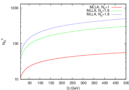
Setting $n_{f}=3$, we display in Fig. 1 our results for the medium-modified MLLA (13) and NMLLA (23) average multiplicity. We plot $N_{g}^{h}$ in the range $10\leq Q(\text{GeV})\leq 500$, where $Q=E\Theta$ is the total virtuality of the jet related to $Y$ in (2). We compare our results in the medium for $N_{s}=1.6$ and $N_{s}=1.8$ (see [5]) with predictions in the vacuum ($N_{s}=1$), we set $Q_{0}=\Lambda_{QCD}=0.23$ GeV in the limiting spectrum approximation [12], and ${\cal K}=0.2$ is taken from [12]. The values $N_{s}=1.6$ and $N_{s}=1.8$ in the medium may be realistic for RHIC and LHC phenomenology [5, 26]; the jet energy subrange $10\leq Q(\text{GeV})\leq 50$ displayed in Fig. 1 has been recently considered by the STAR collaboration, which reported the first measurements of charged hadrons and particle-identified fragmentation functions from p+p collisions [27] at $\sqrt{s_{\text{NN}}}=200$ GeV. Finally, the jet energy range in the same figure, in particular for those values at $Q\geq 50$ GeV, will be reached at the LHC, i.e $Q=100$ GeV is an accessible value in this experiment (see [5] and references therein).

Notice that at NMLLA, the increase of $N_{g}^{h}$ with $N_{s}$ is more substantial than at MLLA. The former is driven by the leading contribution to $\sigma_{2}(N_{s})$: it increases like $\sigma_{2}(N_{s})\simeq N_{s}^{2}$ (see Table 2) in the sub-leading piece of (23). In both resummations schemes we find, as expected from our calculations, that the production of soft hadrons increases as $N_{s}>1$, which implies that the available phase space becomes restricted for the production of harder collinear hadrons.

In Fig. 2, we display the medium-modified MLLA ratio $r=N_{g}/N_{q}$ (18) and the medium-modified NMLLA ratio as a function of $Q=E\Theta$. As expected from (18), as $N_{s}$ increases, the ${\cal O}(\gamma_{0})$ correction is suppressed by $1/\sqrt{N_{s}}$, the ratio approaches the DLA asymptotic regime $r_{0}=N_{c}/C_{F}=9/4$. At NMLLA, the previous trend goes in the opposite direction: one has indeed $-r_{2}(N_{s})\simeq-N_{s}^{2}$ (see Table 2) in the ${\cal O}(\gamma_{0}^{2}/N_{s})$ piece of (26), which is negative and sizable as $N_{s}$ increases and, therefore, spoils the behavior obtained at MLLA signaling difficulties with perturbative theory in the medium. Indeed, sizable oscillations have been noticed in the perturbative series [13] and it turns out that they are wider in the medium than in the vacuum. For example, the NMLLA correction to $r$ is $\sim 10\%$ for $N_{s}=1$, and for $N_{s}=1.8$ it is $\sim 40\%$. It should be noticed that every logarithmic derivative of $N_{A}^{h}$ provides a half power of $N_{s}$ to successive terms in the series in the form $\frac{d^{n}N}{dY^{n}}\approx(N_{s}\alpha_{s})^{n/2}$ ($n=1\to$ MLLA, $n=2\to$ NMLLA…), such that the perturbative approach should fail as higher order terms are incorporated. Former statements suggest that by incorporating NMLLA and next-to-NMLLA (NNMLLA, see paragraph 3.4) corrections on an equal footing, the MLLA behavior can be recovered. We conclude from this analysis that MLLA provides a more realistic physical picture of the softening of jets than NMLLA. Therefore, either the incorporation of NNMLLA terms or the exact numerical solution of the evolution equations [29, 7], which exactly accounts for the running of $\alpha_{s}$ and the energy balance, is required. In [21], a numerical solution of the equations was provided with fixed coupling constant $\alpha_{s}$, and the results are shown to follow our MLLA expectations as $N_{s}$ increases.

Finally, in both MLLA and NMLLA, the gluon jets are still more active than the quark jets in producing secondary particles and the shape of the curves are roughly identical; however, these characteristics prove not to be very sensitive to $N_{s}$.

For $Y\gg\ln x\sim\ln(1-x)$ in the system above (33,36), $N(Y+\ln x)$ ($N(Y+\ln(1-x))$) and $N^{(2)}(Y+\ln x)$ ($N^{(2)}(Y+\ln(1-x))$) can be replaced by $N(Y)$ and $N^{(2)}(Y)$ respectively in the hard partonic splitting region $x\sim 1-x\sim 1$, while the dependence on $\ln x$ is kept on the singular one ($x\to 0$). The medium-modified MLLA approximate system of two-coupled evolution equations for the second multiplicity correlator reads

	$\displaystyle\frac{d^{2}}{dY^{2}}\left(N^{(2)}_{g}-N_{g}^{2}\right)\!\!$	$\displaystyle\!\!=\!\!$	$\displaystyle\!\!\gamma_{0}^{2}\left(N_{s}-a_{1}\frac{d}{dY}\right)N^{(2)}_{g}+(a_{1}-b_{1})\gamma_{0}^{2}\frac{d}{dY}N_{g}^{2},$		(37)
	$\displaystyle\frac{d^{2}}{dY^{2}}\left(N^{(2)}_{q}-N_{q}^{2}\right)\!\!$	$\displaystyle\!\!=\!\!$	$\displaystyle\!\!\frac{C_{F}}{N_{c}}\gamma_{0}^{2}\left(N_{s}-\tilde{a}_{1}\frac{d}{dY}\right)N^{(2)}_{g},$		(38)

where the new hard constant is:

$$b_{1}=\frac{1}{4N_{c}}\left[\frac{11}{3}N_{c}-4\frac{T_{R}}{N_{c}}\left(1-2\frac{C_{F}}{N_{c}}\right)^{2}\right].$$

The constant $N_{s}$ only affects the leading double logarithmic term of the equations. The terms proportional to $a_{1}$, $(a_{1}-b_{1})$ and $\tilde{a}_{1}$ are hard vacuum corrections which partially account for energy conservation, indeed $\gamma_{0}^{2}\frac{dN}{dY}\approx\sqrt{N_{s}}\gamma_{0}^{3}$ and the relative correction to DLA is ${\cal O}(\sqrt{\alpha_{s}/N_{s}})$. As before, the hard constants are, as expected, $N_{s}$-independent. Moreover, these sub-leading contributions have the same form as those describing the two-particle correlation [30].

References

- [1] Yu.L. Dokshitzer, V.A. Khoze, A.H. Mueller & S.I. Troyan, Basics of Perturbative QCD, Editions Frontières, Paris (1991).
- [2]
K. Adcox et al. (PHENIX Collab.), Phys. Rev. Lett. 88
(2002) 022301;
S.S. Adler et al. (PHENIX Collab.), Phys. Rev. Lett. 91 (2003) 072301. - [3] C. Adler et al. (STAR Collab.), Phys. Rev. Lett 89 (2002) 202301.
- [4]
F. Arleo, hep-ph/08101193;
R. Baier, D. Schiff & B. G. Zakharov, Ann. Rev. Nucl. Part. Sci. 50 (2000) 37;
A. Kovner & U. A. Wiedemann, in Quark Gluon Plasma 3, World Scientific, Singapore, hep-ph/0304151;
M. Gyulassy, I. Vitev, X.-N. Wang & B.-W. Zhang, nucl-th/0302077, ibid.;
A. Majumder, J. Phys. G 34 (2007) S377;
For a more recent review, see also S. Peigné & A.V. Smilga, hep-ph/08105702. - [5] N. Borghini & U.A. Wiedemann, hep-ph/0506218.
- [6] N. Armesto, L. Cunqueiro, C. Salgado & W.C. Xiang, JHEP 02 (2008) 048.
- [7] S. Sapeta & U.A. Wiedemann, hep-ph/0809.4251.
- [8] U.A. Wiedemann, Nucl. Phys. B 588 (2000) 303.
- [9] V. N. Gribov & L. N. Lipatov, Yad. Fiz. 15, 781 (1972) [Sov. J. Nucl. Phys. 15, (1972) 438]; G. Altarelli & G. Parisi, Nucl. Phys. B 126, (1977) 298; Yu. L. Dokshitser, Zh. Eksp. Teor. Fiz. 73, (1977) 1216; [Sov. Phys. JETP 46, (1977) 641].
- [10] A.H. Mueller, Nucl. Phys. B 241 (1984) 141; Erratum ibid., B 241 (1984) 141.
- [11] E.D. Malaza & B.R. Webber, Phys. Lett. B 149 (1984) 501; E.D. Malaza & B.R. Webber, Nucl. Phys. B 267 (1986) 702.
- [12] I.M. Dremin & V.A. Nechitailo, Mod. Phys. Lett. A 9 (1994) 1471; JETP Lett. 58 (1993) 945.
- [13] I.M. Dremin, C.S. Lam & V.A. Nechitailo, Phys. Rev. D 61 (2000) 074020.
- [14] G. Abbiendi et al., [OPAL Collaboration], Phys. Rev. D 69 (2004) 032002.
- [15] J. Abdallah et al. [DELPHI Collaboration], Eur. Phys. J. C 44 (2005) 311.
- [16] HRS Coll., Phys. Rev. D 34 (1986) 3304; AMY Coll., Phys. Rev. D 42 (1990) 737; DELPHI Coll., Z. Phys. C-Particles and Fields 50 (1991) 185.
- [17] I.M. Dremin & J.W. Gary, Phys. Rep. 349 (2001) 301.
- [18] D. Acosta et al., Phys. Rev. Lett. 94 (2005) 171802.
- [19] A.N. Safonov (for CDF Collaboration), Nucl. Phys. B (Proc. suppl.) 86 (2000) 55.
- [20] R. Perez-Ramos, F. Arléo & B. Machet, Phys. Rev. D 78 (2008) 014019; F. Arléo, R. Perez-Ramos & B. Machet, Phys. Rev. Lett. 100 (2008) 052002.
- [21] I.M. Dremin, O.S. Shadrin, J. Phys. G 32 (2006) 963.
- [22] N. Armesto, C. Pajares & P. Quiroga Arias, hep-ph/0809.4428.
- [23] Ya.I. Azimov, Yu.L. Dokshitzer, V.A. Khoze & S.I. Troian, Z. Phys. C 27 (1985) 65; Yu.L. Dokshitzer, V.A. Khoze & S.I. Troian, J. Phys. G 17 (1991) 1585.
- [24] R. Perez-Ramos, hep-ph/0811.2418.
- [25] V.A. Khoze & W. Ochs, Int. J. Mod. Phys. A 12 (1997) 2949.
- [26] S. Sapeta & U.A. Wiedemann, Eur. Phys. J. C55 (2008) 293.
- [27] M. Heinz for the STAR Collaboration, nucl-exp/0809.3769.
- [28] Yu.L. Dokshitzer, Phys. Lett. B 305 (1993) 295.
- [29] S. Lupia & W. Ochs, Phys. Lett. B 418 (1998) 214.
- [30] R. Perez-Ramos, JHEP 06 (2006) 019, and references therein; R. Perez-Ramos, JHEP 09 (2006) 014.
- [31] A.M. Polyakov, Sov. Phys. JETP 32 (1971) 296.
- [32] M. Cacciari & G.P. Salam, Phys. Lett. B 641 (2006) 57.
- [33] ALICE collaboration, B. Alessandro et al., J. Phys. G 32 (2006) 1295.
- [34] CMS collaboration, D. d’Enterria (Ed.) et al., J. Phys. G 34 (2007) 2307.