The University Of British Columbia \institutionaddressVancouver, Canada \programPhysics \numberofsignatures4 \previousdegreeB.Sc., The Chinese University of Hong Kong, 2001 \previousdegreeM.Phil., The Chinese University of Hong Kong, 2003 \ubclocationVancouver \submitdateAugust, 2008 \advisorDouglas Scott \advisortitleProfessor of Astronomy
Cosmological Recombination
Abstract
In this thesis we focus on studying the physics of cosmological recombination and how the details of recombination affect the Cosmic Microwave Background (CMB) anisotropies. We present a detailed calculation of the spectral line distortions on the CMB spectrum arising from the Ly and two-photon transitions in the recombination of hydrogen (H), as well as the corresponding lines from helium (He). The peak of these distortions mainly comes from the Ly transition and occurs at about m, which is the Wien part of the CMB. The detection of this distortion would provide the most direct supporting evidence that the Universe was indeed once a plasma.
The major theoretical limitation for extracting cosmological parameters from the CMB sky lies in the precision with which we can calculate the cosmological recombination process. Uncertainty in the details of hydrogen and helium recombination could effectively increase the errors or bias the values of the cosmological parameters derived from microwave anisotropy experiments. With this motivation, we perform a multi-level calculation of the recombination of H and He with the addition of the spin-forbidden transition for neutral helium (He i), plus the higher order two-photon transitions for H and among singlet states of He i. Here, we relax the thermal equilibrium assumption among the higher excited states to investigate the effect of these extra forbidden transitions on the ionization fraction and the CMB angular power spectrum . We find that the inclusion of the spin-forbidden transition results in more than a percent change in , while the higher order non-resonance two-photon transitions give much smaller effects compared with previous studies.
Lastly we modify the cosmological recombination code recfast by introducing one more parameter to reproduce recent numerical results for the speed-up of helium recombination. Together with the existing hydrogen ‘fudge factor’, we vary these two parameters to account for the remaining dominant uncertainties in cosmological recombination. By using a Markov Chain Monte Carlo method with Planck forecast data, we find that we need to determine the parameters to better than 10% for He i and 1% for H, in order to obtain negligible effects on the cosmological parameters.
Chapter 0 List of Symbols
| Case B recombination coefficient of species x | |
| Case B photoionization coefficient of species x | |
| Variance of the comoving curvature perturbations | |
| Wavelength of a photon | |
| Cosmological constant | |
| Spontaneous 2s–1s two-photon rate of H i | |
| Spontaneous 21S0–11S0 two-photon rate of He i | |
| Spontaneous two-photon rate of species x from th state to th state | |
| Chemical potential in the radiation spectrum | |
| Frequency of a photon | |
| Critical density (zero curvature) | |
| Ratio of dark energy density to the critical density | |
| Ratio of baryon density to the critical density | |
| Ratio of cold dark matter density to the critical density | |
| Ratio of total matter density to the critical density | |
| Ratio of total density of the Universe to the critical density | |
| Thomson scattering cross-section | |
| Ionization cross-section at frequency | |
| Optical depth | |
| Radiation constant, | |
| Amplitude of spherical harmonic component | |
| Scalar amplitude of the primordial perturbation | |
| Einstein coefficient of transition from th to th state | |
| Einstein coefficient of transition from th to th state | |
| Fudge factor for He i recombination | |
| Speed of light | |
| CMB anisotropies at angular moment | |
| Ionization energy of the th state in an atom | |
| Total internal energy of a system with matter and radiation | |
| Number fraction of helium nuclei, | |
| Fudge factor for speeding up the H i recombination at low redshift | |
| Newton’s gravitational constant | |
| Degeneracy of the th state in an atom | |
| Visibility function for the CMB photons | |
| Hubble parameter, expansion rate of the Universe, |
| Current value of Hubble constant | |
| Dimensionless value of , /100 km s-1 Mpc-1 | |
| Planck’s constant | |
| Specific intensity per unit frequency | |
| Specific intensity per unit wavelength | |
| Specific intensity per unit frequency from a blackbody | |
| Wavenumber or inverse scale of primodial fluctuation | |
| Boltzmann’s constant | |
| Multipole of the CMB temperature fluctuation | |
| Angular momentum of a level in an atom | |
| Mpc | Mega-parsec ( pc), 1 pc = 3.26156 light years = 3.0857 m |
| Electron mass | |
| Proton mass | |
| Mass of hydrogen atom | |
| Mass of helium 4He atom | |
| Principle quantum number of a level in an atom | |
| Number density of nucleus of species x | |
| Number density of electrons | |
| Number density of electrons in the th level of atom x | |
| Index of power spectrum of primodial fluctuations | |
| Sobolev escape probability of photons | |
| Scale factor for universal expansion | |
| Net transition rate from th state to th state of species x | |
| Matter temperature | |
| Radiation temperature | |
| Current radiation temperature, | |
| Radiation energy density | |
| Ionization fraction or free electron fraction, | |
| Compton-scattering distortion parameter | |
| Primordial mass fraction of 4He | |
| Spherical harmonics | |
| Redshift |
Acknowledgements.
First I would like to thank my supervisor, Douglas Scott for his ideas, encouragement and patience. He introduced me to the field of cosmology and guided me through my research projects. I have learned a lot through stimulating discussions with him and he always shares his ideas openly in different aspects of physics and astronomy. I would also like to thank the other collaborators in this work. Sara Seager generously shared her original numerical recombination code and shared with me her understanding of recombination. She also provided me hospitality during my stay at the Carnegie Institute of Washington. And Adam Moss helped me to make the CosmoMC code work properly. I would like to thank the Astronomy group at the University of British Columbia. The professors provided an interactive, warm and helpful environment for me to study here. And the graduate students, especially my officemates, gave me a sense of what is Canadian culture. I would also like to thank the staff in St. John’s College, especially the kitchen chefs. They provided me with a comfortable stay and wonderful meals during my two years of living there. Here I would also like to thank my friends for all their support. In particular, Kandy Wong and Cecilia Mak always help me out and bring lots of fun to my life in Vancouver. I owe my father and mother many thanks. They brought me into this amusing world and allowed me to do whatever I like to do. I thank my brother Ting Chun Wong for taking care of the family when I am away from home. And to my husband Henry Ling. He always supports and helps me through the difficult times.Chapter 0 Co-Authorship Statement
This thesis is in the manuscripted format and Chapters 3 to 6
are essentially reprints of individual published works (see the footnotes of
the first page in each chapter for references).
My supervisor, Professor Douglas Scott provided many useful
discussions during all of these works and also gave me numerous
suggestions in editing the papers, but in each case
the calculations and writing are on my own.
Chapter 3
Professors Sara Seager and Douglas Scott are the co-authors of the work in
Chapter 3, and initiated this project.
The numerical recombination code was originated and
developed by Professor Sara Seager before this work started.
I performed all the calculations by modifying the relevant parts in
the numerical code, analyzed the results and wrote the manuscript.
Chapter 4
Professor Douglas Scott is the co-author of the work in Chapter 4, and
motivated me to start this project. I collected and updated the atomic data
in the numerical code originally developed by Professor Sara Seager.
Modifications were made in the numerical code specifically for
the study in this Chapter. I performed all
the theoretical and numerical calculations, analyzed the results
and wrote the manuscript.
Chapter 5
Professor Douglas Scott is the co-author of the work in Chapter 5, and
motivated me to clarify this previous claimed effect on the recombination
calculation. I developed the consistent approach
under the equilibrium assumption and also estimated the maximum
effect in the real situation. I also wrote the manuscript of this work.
Chapter 6
Professor Douglas Scott and Dr. Adam Moss are the co-authors of the
work in Chapter 6. Professor Douglas Scott motivated me to start
this project. I developed the method and modified the
existing recfast recombination code by including the
recent updates and uncertainties. Dr. Adam Moss provided the
Planck forecast data and helped me in running the
CosmoMC code. I performed all the numerical calculations,
analyzed the results and wrote the paper.
Chapter 0 Introduction
The detection of the 2.725 K Cosmic Microwave Background (CMB) is one of the strongest pieces of supporting evidence for the Big Bang model, which is the widely accepted theory for the history of the Universe. Together with other observations, we know that the Universe is expanding implying that it was much denser and hotter in the past and used to be a plasma of ions and electrons. The CMB, which is the remnant of the early radiation, was last scattered when the atoms became neutral. This period is called cosmological recombination, and it happened when the Universe was a few hunderd thousand years old. In the decades following its discovery, the CMB was found to be remarkably homogeneous and isotropic, but its tiny temperature fluctuations give us the most distant image we have of the Universe. This carries important information about the geometry, the expansion rate and contents of the Universe, as well as clues about the origin of all the structure it contains (see, for example, [21, 24]). Exploiting this information requires an extremely precise undertanding of the process of cosmological recombination, which is the main topic of this thesis. In order to explain why this is the case we should first review the physics of the standard cosmological model.
0.1 A brief history of the Universe
In the late 1920s, Hubble [14] discovered that the Universe is expanding. He found that atomic lines in the spectrum of nearly all distant galaxies are redshifted (or shifted to longer wavelengths) compared with the laboratory values. This means that the galaxies are moving away from us due to the expansion of the Universe. The redshift is defined as
| (1) |
where and are the observed and emitted wavelengths, respectively. Here is a time-dependent scale factor, which gives infinitestimal distances in space when multiplied by the comoving distance . This idea of a uniform scale factor for the expansion is consistent with Hubble finding that the velocity of galaxies increases linearly with distance , which is the famous Hubble’s law:
| (2) |
Here is the Hubble constant and represents the rate of expansion so that
| (3) |
and today we have . Although the actual value of the constant determined by Hubble is far from our current estimates, the Hubble diagram nevertheless proves that the Universe is expanding, and the same principle is used for today’s measurements: measure the redshifts and estimate the distances of distant objects to determine . Redshift, can be easily estimated from the shifting of the spectral lines, but it is hard to determine the distances without any information of on the intrinsic brightness or the intrinsic size of an object, so that precision measurements of Hubble’s constant have been elusive.
The current value of the Hubble constant (the subscript ‘0’ represents the present value, that is at = 0) was determined by the Hubble Key Project [7] using ‘standard candles’, which basically have the same intrinsic brightness or have a correlation between some observables and the intrinsic brightness. For example, Cepheid variables and Type Ia supernovae are commonly used standard candles. The measured value of is equal to km s-1Mpc-1 [7]. We usually define a dimensionless constant for , which is
| (4) |
and therefore, = 0.72 0.08. Assuming is constant, the age of the Universe is then equal to , which is about 13.7 Gyr.
The Universe appears to be homogeneous and isotropic on large scales (distances greater than about 300 Mpc) from observations of the distribution of galaxies [23]. This is the Cosmological Principle; based on that we can build a simple model of the expanding Universe within General Relativity. Here we temporarily ignore the density fluctuation on small scales, which are of small amplitude in the early Universe but important later for the formation of galaxies and clusters (the structure formation). On large scales, the Universe can be described by the Friedmann-Robertson-Walker (FRW) metric and the geometry of the Universe depends on the total density (see, for example, [21, 24]). Given the expansion rate , there is a critical density that determines whether the Universe has flat geometry. This critcal density is
| (5) |
and we usually define a density parameter
| (6) |
where represents different components (e.g. matter, radiation and dark energy) in the Universe. The Universe is spatially closed if the total density of the Universe is larger than , and spatially open if its density is lower than .

From the combined results of recent observations of the CMB, acoustic signatures in galaxy clustering and Type Ia supernovae, the Universe is found to be very close to flat with the total density 1.0052 0.0064 [9]. At the present time the Universe consists of about 4% baryons (), 20% cold dark matter (), 76% dark energy () and a tiny portion of photons ( 4.17 ). Here ‘baryon’ means ordinary matter, for example atoms, nuclei and electrons. ‘Dark matter’ is some gravitationally interacting (weakly interacting with baryons) and non-luminous substance. The dark matter is considered to have velocity dispersion which is negligible for structure formation, meaning that it decoupled when it was non-relativistic (cold); its fluctuations are the seeds of structure formation. The concept of dark matter was first proposed by Zwicky [45] in 1933 through observations at the rotational curves of stars in galaxies. This dark matter was introduced in order to explain the increasing rotational velocity of material with increasing distance from the centres of galaxies. As we will see later, since Big Bang Nucleosynthesis (as well as the CMB) gives a very low limit on the baryon density, some non-baryonic matter must exist in the Universe. In general, the density of matter is proportional to , while that of the radiation is proportional to . The dark energy provides the negative pressure responsible for the recent accelerated expansion of the Universe and its density is constant over redshift (this is Einstein’s cosmological constant, ) or very nearly so.
Due to different scalings of the density of each species with redshift, the components dominate the Universe at different times. Figure 1 shows a brief history of the Universe and indicates the important epochs using both time and redshift as coordinates. In cosmology, redshift is usually used instead of time, since it is (in principle at least) directly observable and so independent of the cosmological model. In the Big Bang picture, the very early times are still quite uncertain, but the physics of the thermal history of the Big Bang Nucleosynthesis (BBN) and recombination are well understood and firmly established.
The earliest times were radiation dominated. The Universe was very hot (the background radiation temperature = , where = 2.725 K) and dense. Due to the strong and highly energetic photon background, there were no bound nuclei until BBN occured at about 3 minutes after the Big Bang (). During BBN, the temperature decreased to about 100 keV/, which is lower than the typical binding energy of the nuclei. Therefore, nuclei of deuterium (D), helium (3He, 4He) and lithium (7Li) were able to form without being destroyed by the photons. Given the baryon density , the theoretical calculation of standard BBN can predict the abundance of different species of nuclei with very small uncertainties due to nuclear and weak-interaction rates (see Figure 1 in [2] or Figure 5 in [35]). In particular, the abundance of D is very sensitive to . By measuring the primodial abundance of D through the absorption lines in the hydrogen clouds at redshift , we can put tight constraints on using the theoretical BBN prediction (see [2] and references therein). BBN gives a limit that the baryons can contribute at most 5% of the critical density, and therefore the rest of the matter must be non-baryonic.
At about years () after the Big Bang, the radiation temperature dropped to around 1 eV/, which is lower than the ionization energy of typical atoms. This period is called cosmological recombination. During this time, the ions and electrons were able to bind together without being ionized by the background photons. After the Universe became neutral, the photons were no longer scattered by the electrons and could basically travel freely to the present, being redshifted in the expanding Universe. These are the CMB photons that we detect today. The CMB has been found to be remarkably smooth, the amplitude of the temperature deviations is only about , which is a strong contrast to the non-linear structure formed by the galaxies and clusters we observe today. Therefore this fluctuation amplitude of temperatures in the CMB gives us an idea about the strength of the matter density fluctuations at the time of recombination, which evolved into the large scale structures we observe now.
After recombination, the Universe remained dark and neutral until the first stars formed. There has not been any detection of informtion from this ‘dark age’ and we are still not sure how and when exactly the first stars formed. Up until now, the most distant quasar that has been observed is at about [15, 42]. From the hydrogen absorption line spectra from such high- quasars [1] we know that the Universe was fully ionized by ultraviolet radiation from hot stars at . Moreover the CMB provides a constraint on the optical depth during this reionization epoch through the Thomson scattering effect on the photons. The integrated optical depth is
| (7) |
where is the Thomson scattering cross-section, is the number density of free electrons and is the redshift at which the Universe became ionized. From the latest CMB measurement and assuming that the Universe became fully ionized instantaneously, the current estimate is 11 [9]. Stars and galaxies are created basically due to the gravitation collapse of dense regions, but the process is non-linear and also involves the pressure of the gas. Therefore, although the current matter inhomogeneites in the Universe and the temperture fluctuations of the CMB originated from the same source, they appear very different today.
In inflationary models, the primodial perturbations are generated by quantum fluctuations (see [21, 24] for a general review). For the simplest model, by assuming the matter is adiabatic and its fluctuations are Gaussian, the initial conditions for density perturbations can be described by only two parameters: the scalar amplitude and the spectrum index (the slope of the power spectrum; the subscript ‘s’ distinguishes these scalar perturbations from possible tensor, or gravity wave, contributions). The variance of the comoving curvature perturbations is usually defined as [27]
| (8) |
where , is the wavenumber and Mpc-1.
Since the CMB photons come from the time before stars formed, the anisotro-pies in the CMB provide us with information about density perturbations at the recombination time and in combination with measurements made today, they are a powerful tool for constraining the parameters of the cosmological model. From the above discussion, and assuming a flat Universe, the standard cosmological model (the Cold Dark Matter model, CDM) consists of six parameters: , , , , and . There could of course be more parameters in the cosmological model (see [17] for a review), for example, including the tensor mode of the primodial perturbations or allowing the Universe to deviate from flatness ().
Since the CMB photons were mostly last scattered during the epoch of cosmological recombination, we need to understand in detail how the photons decoupled from the matter during that period in order to obtain the correct CMB anisotropy power spectrum for constraining the cosmological parameters using the observations. In this thesis, we focus on the physics of recombination and how the details of the recombination process affects the CMB. We now therefore present an introduction to the physics of cosmological recombination (the last scattering surface of the CMB photons), and also the basic principles of the formation of the CMB anisotropies.
0.2 Cosmological recombination
Recombination in an expanding Universe is not an instantaneous process. It is basically controlled by the recombination time and by the Hubble expansion time. If the recombination time is much shorter than the expansion time, then the electrons and ions follow an equilibrium distribution. For the ionization of a plasma, the equilibrium situation is described by the Saha equation. Taking hydrogen as an example (see Equation (13) in [29] and references therein),
| (9) |
Here is the number density of electrons in the th energy level of the H atom, is the number density of free protons, is the mass of the electron, is the Boltzmann constant, is Planck’s constant, is the degeneracy of the energy level and is the ionization energy of level . Due to the higher ionization energy, helium recombined at higher redshifts, first by forming He+ (He ii) and then neutral He (He i). Hydrogen started to recombine shortly after. Figure 2 shows the full ionization history of recombination by plotting the ionization fraction ( , where is the number density of H nuclei) versus . Based on standard BBN, about 8% (by number) of the atomic nuclei are helium. And since the ionization fraction is normalized to the total number density of hydrogen, is equal to about 1.16 when the Universe is fully ionized.
Peebles (1968) [22] and Zeldovich (1968) [44] first calculated the H i recombination evolution in detail and found that the recombination process is much slower than Saha equilibrium (for example, see Figure 6.8 in [24]). The Saha equation is good for describing the initial departure from full ionization, but the equilibrium situation breaks down shortly after recombination starts. When the temperature of the Universe reached about 0.3 eV/ at 1700, there were not enough photons in the Wien tail to keep ionizing the H atoms. Due to the high photon to baryon ratio , direct recombinations to the ground state were highly prohibited. The ‘spectral distortion’ photons emitted from direct recombination are highly energetic and easily re-ionize the nearby neutral atoms. This is very similar to the ‘Case B’ recombination familiar in other areas of astrophysics (see e.g. [20]), in which the electrons mostly cascade down to the ground state through the first excited state = 2. However, in cosmological H i recombination, the resonant 2p–1s Ly transition is also strongly suppressed, because the line is optically thick. These line photons can only escape reabsorption through redshifting out of the line and the probability for this is very low. The other way for the electrons to move from the first excited state to the ground state is through the 2s–1s two-photon forbidden transition. Almost half of the electrons cascade down from the = 2 state through this process (see Chapter 2 & 3 for details). Overall, the net recombination rate to ground state from = 2 state is lower than the recombination rate into the = 2 state, and this causes a ‘bottleneck’, which is responsible for making the net recombination rate much smaller than the one given by Saha equilibrium.

In the next chapter, we will discuss details of the radiative processes during recombination and also recent development in performing the numerical calculations. However, all the updates are based on the basic picture of the standard recombination given here. We have already discussed how H i recombination is not an equilibrium process. The situation is similar for helium recombination. He i recombination is also slower than Saha equilibrium due to the ‘bottleneck’ at the first excited state, but He ii deviates from the Saha value at only the 0.2% level due to the relatively fast two-photon rate to the ground state [29, 39].
The ionization fraction affects the CMB anisotropies (see Equation (13) for the definition of ) through the shape of the last scattering surface which is given by the visibility function ,
| (10) |
where is the Thomson optical depth during recombination (excluding the effects of reionization if we are only considering primary anisotropies). Here is defined the same as in Equation (7), but with different integration limits (say, from = to 100). One can consider as the probability that a photon last scattered at redshift . In Figure 2, the function is plotted on top of the ionization history of cosmological recombination. Since changes rapidly with , is sharply peaked, and its width gives us the thickness of the last scattering surface (which means that the CMB photons we see last scattered in the specific range of redshift 600 1500). It is usual to define the location of the peak of as the redshift of the recombination epoch, when the radiation effectively decoupled from the matter . This is approximately equal to 1100 in the current cosmological CDM model. From the profile of , we can see that H i recombination affects the much more than He. The later stages of He i recombination can also change the high- tail of (see Chapter 6 for more details), but He ii recombination occurs too early to bring any significant effects on .
0.3 Cosmic microwave background
From many measurements, particularly those of the Far-InfraRed Absolute Spectrophotometer (FIRAS) on board with the Cosmic Background Explorer (COBE) [5, 6, 19], the CMB was found to be very close to a pure blackbody spectrum, which is described by the Planck function :
| (11) |
Figure 3 shows the data points from FIRAS [5, 6], with error bars multiplied by 100 and compared with the theoretical blackbody spectrum with = 2.725 K. We can see that the data points match the blackbody shape incredibly well within the frequency range from 2 to 20 cm-1 (i.e. 60 to 600 GHz). The deviation is less than 5 at the peak of the CMB spectrum [5]. The background photons originate from an epoch much earlier than that of recombination, coming from the electron-positron annihilations before BBN and from when the energy of the photons was so high that bremsstrahlung and double Compton scattering could create and destroy photons so that they were rapidly thermalized into a blackbody spectrum [36]. Hence spectral distortion constrain any energy injection later than that epoch. The FIRAS data put strong limits on the chemical potential 9 and the Compton-scattering distortion parameter 1.5 [5, 37]. These strong constraints eliminated many earlier competing cosmological models and provide strong evidence that the radiation temperature scales accurately as (1 + ) (see, for example, [21, 43] for more details). The small value of shows that the hydrogen remained neutral for quite a long time, otherwise distortions of the blackbody spectrum due to Compton scattering by the hot electrons would be observed (see [37] and references therein).

The other main feature of the CMB is the dipole variation of the temperature across the sky, with an amplitude equal to 3.358 mK (see [27] for a review). This anisotropy is determined by the Doppler shift from the solar system’s motion relative to the ‘rest frame’ of the radiation, which is supported by measurements of the radial velocities of relatively local galaxies. When we talk about the temperature anisotropies of the CMB, this contribution from our relative motion is usually removed.
The first detection of the CMB temperature anisotropies was made by the COBE Differential Microwave Radiometer (DMR; [33]). The variations in temperature, , were found to be of the order of . We usually decompose maps of the CMB temperature fluctuations using the spherical harmonic expansion:
| (12) |
If the fluctuations are Gaussian and the sky is statistically isotropic (independent of ), then the temperature field is fully charaterized by the amplitudes ,
| (13) |
We usually plot , since this is the contribution to the variance of the power spectrum per logarithmic interval in (see, for example, [13, 27, 41]). The radiation temperature itself corresponds to the monopole , while the dipole variation corresponds to .
Temperature fluctuations in the CMB are essentially a projection of the matter density perturbations at the recombination time. There are many reviews covering details of the formation of the CMB anisotropies (see [13, 27] and references therein) and we just briefly recount the basic mechanism here. Photons from high density regions were redshifted when they climbed out of the potential wells (the Sachs-Wolfe effect). And the adiabaticity between matter and photons also gives a higher temperature in higher density regions. The other primary source is the oscillating density and velocity of the photon fluid itself. Before the epoch of recombination, the baryons and the radiation are tightly coupled as a single photon-baryon fluid, through Thomson and Compton scatterings. The structure seen in the anisotropy power spectrum is mainly due to the acoustic oscillations in this photon-baryon fluid, driven by the evolving perturbations in the gravitational potential. One can think of these oscillations as standing waves in a harmonic series, with the fundamental mode being the scale which has reached maximal compression at the time of last scattering. After recombination, when the Universe became neutral, the photons decoupled from the atoms and could propagate freely to us (although there are some secondary anisotropies formed when the photons travel along the line of sight). Therefore, the correct interpretation of the relationship between the underlying matter fluctuation spectrum and the photon distribution depends strongly on the angular diameter distance between us and the last scattering surface. This distance depends on the expansion and curvature of the Universe or equivalently, the energy content of the Universe. Therefore, the CMB temperature anisotropies can provide precise constraints on the cosmological expansion model, as well as the scale dependence of the primodial fluctuations.
In addition, the Thomson scattering between electrons and photons also leaves a characteristic signature in the polarization of the CMB photons. The quadrupole temperature anisotropy in the photon field generates a net linear polarization pattern through Thomson scattering. It has became conventional to decompose the polarization pattern into two modes: a part that comes from a divergence (‘E-mode’); and another part from a curl (‘B-mode’). Scalar perturbations (i.e. spatial variations in density) coming from the inflation epoch only give an E-mode signal, while tensor perturbations (i.e. gravity waves) produce both E and B-modes. Much current activity in CMB experiments is focussed on trying to measure these B-modes, in order to probe the physics of inflation. In fact, there are 6 possible cross power spectra from the full temperature and polarization anisotropy data set. Cross-correlation between the B-mode and either the T or E-mode is zero due to having opposite parity. This leaves us with 4 possible observables: , , and .
Figure 4 shows the anisotropies and with 2 from recent result based on the Wilkinson Microwave Anisotropy Probe (WMAP; [9]) 5-year data. The points show the WMAP data, while the solid line is the best-fit CDM model. We can see that the first two acoustic peaks of the temperature spectrum are well measured and there is clearly a rise for the third peak. Together with other ground based experiments (see [27] and references therein), perhaps the first five acoustic peaks have now been localized.
The amplitude of the polarization signal is about 2 orders of magnitude smaller than the temperature one and so it is much harder to detect. The DASI [16] experiment first demonstrated the existence of CMB polarization in 2002 and the WMAP experiment has measured the TE power spectrum to high precision [9]. Figure 4 shows the recent measurements of from the WMAP 5 year results.

0.4 Why are we interested in recombination?
0.4.1 Distortion photons from recombination
From the previous section, we know that the photons in the radiation background were thermalized to a nearly perfect blackbody spectrum by bremsstrah-lung and double Compton scattering processes before recombination. As well as the photons from this blackbody background, there were some extra distortion photons produced during the epoch of cosmological recombination. When an electron combined with an ionized atom and cascaded down to the ground state, there was at least one distortion photon emitted for each recombination. These recombination photons give a distinct series of spectral line distortions on the nearly perfect blackbody CMB spectrum. The main contribution to the distortion comes from the H i Ly transition at about , and this line will be observed in the Wien tail ( m) of the CMB spectrum today (see Figure 7 in Chapter 3). Since these distortion photons are produced directly from each recombination of the atoms, the overall shape and amplitude of the line are very sensitive to the details of the recombination process. Therefore the detection of this spectral distortion would provide direct contraints on the physics of recombination and also provide incontrovertible evidence that the Universe was once a hot, dense plasma which recombined.
FIRAS showed that the CMB spectrum around the peak is well-modelled by a 2.725 K Planck spectrum. It was found that there is also a Cosmic Infrared Background (CIB; see [3, 8, 26]), which peaks at about 150 m, right above the recombination distortion on the CMB spectrum (see Figure 7). This background is mainly due to luminous infrared galaxies at fairly recent epochs and it makes the detection of the recombination distortion even more challenging. The first calculations of the line distortion on the CMB tail were presented by Peebles (1968) [22] and by Zeldovich et al. (1968) [44]. However, they provided no details about the line shape, and since then there have been no explicit calculations showing different contributions to the line shape. Today we have a better understanding of the cosmological model as well as improved detection techniques, and so it is time to calculate these spectral distortion lines to much higher accuracy, in order to investigate whether they could be detected and whether such a detection would be cosmologically interesting. A detailed study of this line distortion on the CMB spectrum coming from the recombination time will be presented in Chapter 3.
0.4.2 Precision cosmology
The CMB anisotropies have been well studied theoretically, and the calculations are robust, because they can be based on linear perturbation theory (see [13] and references therein), given that the primordial fluctuations are of small amplitude. CMBFAST [31] is one of the most widely used numerical Boltzmann codes for calculating the . It has been tested over a large set of cosmological models and is consistent with other codes with an accuracy at better than the 1% level [32]. We have already entered the era of precision cosmology [11, 25, 34, 40]. With the release of the WMAP 5 year data, we can constrain the cosmological parameters extermely well from the shape of the anisotropy power spectrum [9]. The next generation of CMB satellites, Planck [25], which will be launched in early 2009, has been designed to sensitively measure the of the TT- and TE-modes up to = 2500 and the EE-mode for . In order to extract the correct cosmological parameters from the experimental data, theoretical calculations with consequently higher accuracy are required. It now seems clear that we need to obtain the theoretical s to better than the 1% level. And the main theoreical uncertainty comes from details of the ionization history during recombination [32].
recfast [28] is the most common numerical code for calculating the evolution of the ionization fraction during recombination; it is embedded into all of the widely-used Boltzmann codes. It is written to be a short and quick program for reproducing the results from a multi-level atom calculation [29], which follows the evolution of the number density of electrons at each of more than 100 atomic levels for each species of atom. The accuracy of the obtained from recfast is at the percent level, which is sufficient for WMAP, but may not be good enough for Planck. This fact has recently motivated many researchers to investigate several detailed physical processes during recombination which may cause roughly percent level changes on . Although the basic physical picture for standard cosmological recombination is quite well established, the non-equilibrium details of recombination are unexpectedly complicated to solve. That is because it must be done consistently with the interaction between the matter and radiation field, in order to reach the required sub- 1% accuracy in (see Chapter 2 for a review). In one specific example (Chapter 4), we investigated the effect of inclusion of the higher order non-resonant two-photon transitions and the semi-forbidden transitions in a multi-level atom calculation, which was first suggested by Dubrovich & Grachev (2005) [4] using a three-level atom model.
There have recently been comprehensive studies of calculations of the He i reombination, with all relevent radiative processes to the 0.1% accuracy level [10, 38, 39]. However there still has not been a single numerical calculation which includes all the improvements in H i recombination (which of course has greater effect on the than for He). From another point of view, given the precision of the experimental measurement, we may want to ask how accurate the theoretical model needs to be in order not to bias the determination of the cosmological parameters. In another of our projects (Chapter 6), we investigated how the remaining uncertainties in recombination affects the constraints on the cosmological parameters using Planck forecast data. We do this through use of the CosmoMC code [18], which is a numerical code for exploring the multi-dimensional cosmological parameter space with the Markov Chain Monte Carlo method.
0.5 Outline of the thesis
This thesis focuses on the study of cosmological recombination and its effects on the CMB. Here we have briefly reviewed the standard model for the evolution of Universe, including the basic picture of cosmological recombination and the formation of the CMB. Chapter 2 provides an overview of progress in the theoretical calculation of recombination, and the recent updates for obtaining the ionization fraction to better than 0.1% accuracy. In Chapter 3 we present a calculation of the spectral distortions in the CMB due to H i Ly and the lowest 2s–1s line transitions, as well as the corresponding lines of He i and He ii, during the epoch of recombination. Next, in Chapter 4, we investigate the effects of including non-resonant two-photon transitions and the semi-forbidden transitions in the process of H i and He i recombination. Chapter 5 is a brief study to clarify that the previously claimed effect of the reheating of matter due to the distortion photons emitted during recombination is neligible. In Chatper 6 we investigate how uncertainties in the recombination calculation affects the determination of the cosmological parameters in future CMB experiments. Finally we present our conclusion and ideas for future directions in Chapter 7.
0.6 References
References
- [1] Becker R. H., et al. 2001, Astrophysical Journal, 122, 2850
- [2] Burles S., Nollett K. M., Truran J. W., Turner M. S. 1999, Physical Review Letters, 82, 4176
- [3] Dole H., et al. 2006, Astronomy and Astrophysics, 451, 417
- [4] Dubrovich V. K., Grachev S. I. 2005, Astronomy Letters, 31, 359
- [5] Fixsen D. J., Cheng E. S., Gales J. M., Mather J. C., Shafer R. A., Wright E. L. 1996, Astrophysical Journal, 473, 576
- [6] Fixsen D. J., Mather J. C. 2002, Astrophysical Journal, 581, 817
- [7] Freedman W. L., et al. 2001, Astrophysical Journal, 553, 47
- [8] Hauser M. G., Dwek E., 2001, Annual Review of Astronomy and Astrophysics, 39, 249
- [9] Hinshaw, G., et al. 2008, ArXiv e-prints, arXiv:0803.0732
- [10] Hirata C. M., Switzer, E. R. 2008, Physical Review D, 77, 083007
- [11] Hu W. 2000, Nature, 404, 939
- [12] Hu W., Scott D., Sugiyama N., White M. 1995, Physical Review D, 52, 5498
- [13] Hu W., Dodelson S. 2002, Annual Review of Astronomy and Astrophysics, 40, 171
- [14] Hubble E. 1929, Proceedings of the National Academy of Science, 15, 168
- [15] Jiang L., et al. 2008, Astronomical Journal, 135, 1057
- [16] Kovac J. M., Leitch E. M., Pryke C., Carlstrom J. E., Halverson N. W., Holzapfel W. L. 2002, Nature, 420, 772
- [17] Lahav O., Liddle A. R. 2006, in ‘The Review of Particle Physics’, Yao W.-M. et al., Journal of Physics, G 33, 1, arXiv:astro-ph/0601168
- [18] Lewis A., Bridle S. 2002, Physical Review D, 66, 103511
- [19] Mather J. C., et al. 1994, Astrophysical Journal, 420, 439
- [20] Osterbrock D. E., Ferland G. F. 2006, Astrophysics of Gaseous Nebulae and Active Galactic Nuclei, University Science Books
- [21] Peacock J. A. 1999, Cosmological Physics, Cambridge University Press, Cambridge, UK
- [22] Peebles P. J. E. 1968, Astrophysical Journal, 153, 1
- [23] Peebles P. J. E. 1980, The Large scale Structure of the Universe, Princeton University Press, Princeton, New Jersey, USA
- [24] Peebles P. J. E., 1993, Principles of Physical Cosmology, Princeton University Press
- [25] The Planck Collaboration 2006, ESA-SCI(2005)1, arXiv:astro-ph/0604069
- [26] Puget J.-L. et al., 1996, Astronomy and Astrophysics, 308, L5
- [27] Scott D., Smoot G. F. 2006, in ‘The Review of Particle Physics’, Yao W.-M. et al., Journal of Physics, G 33, 1, arXiv:astro-ph/0601307v1
- [28] Seager S., Sasselov D. D., Scott, D. 1999, Astrophysical Journal, 523, L1
- [29] Seager S., Sasselov D. D., Scott D. 2000, Astrophysical Journal Supplement, 128, 407
- [30] Seager S. 2001, Spectroscopic Challenges of Photoionized Plasmas, ASP Conference Series Vol. 247. Edited by Gary Ferland and Daniel Wolf Savin. San Francisco: Astronomical Society of the Pacific, 327
- [31] Seljak U., Zaldarriaga M. 1996, Astrophysical Journal, 463, 1
- [32] Seljak U., Sugiyama N., White M., Zaldarriaga M. 2003, Physical Review D, 68, 083507
- [33] Smoot G. F. et al. 1992, Astrophysical Journal Letters, 396, L1
- [34] Spergel D. N. et al. 2003, Astrophysical Journal Supplement, 148, 175
- [35] Steigman G. 2007, Annual Review of Nuclear and Particle Science, 57, 463
- [36] Sunyaev R. A., Zeldovich Y. B. 1970, Astrophysics and Space Science, 7, 20
- [37] Sunyaev R. A., Zeldovich I. B. 1980, Annual Review of Astronomy and Astrophysics, 18, 537
- [38] Switzer E. R., Hirata C. M. 2008, Physical Review D, 77, 083006
- [39] Switzer E. R., Hirata C. M. 2008, Physical Review D, 77, 083008
- [40] Turner M. S. 2001, The Publications of the Astronomical Society of the Pacific, 113, 653
- [41] White M., Scott D., Silk J. 1994, Annual Review of Astronomy and Astrophysics, 32, 319
- [42] Willott C. J., et al. 2007, Astronomical Journal, 134, 2435
- [43] Wright E. L., et al. 1994, Astrophysical Journal, 420, 450
- [44] Zeldovich Y. B., Kurt V. G., Syunyaev R. A. 1968, Zhurnal Eksperimental noi i Teoreticheskoi Fiziki, 55, 278: English translation: 1969, Soviet Physics-JETP, 28,146
- [45] Zwicky, F. 1933, Helvetica Physica Acta, 6, 110
Chapter 0 Progress in recombination calculations11 1 A version of this chapter will be submitted for publication: Wong W. Y. ‘Progress in recombination calculations’.
In this chapter, we will give a review of progress in controlling the accuracy of the recombination calculation, starting from a traditional three-level atom model and going up to the recent multi-level atom models including interactions between matter and radiation. We will also describe the remaining uncertainties which will need to be tackled in the numerical codes in order to obtain the ionization fraction to better than 1%.
0.7 Standard picture of recombination
Cosmological recombination calculations were first performed forty years ago by Peebles (1968) [63] and Zeldovich, Kurt and Sunyaev (1968) [88] using a 3-level atom model in hydrogen ( + e- H + ). In this simplified model, one only follows the detailed rates of change of electrons in the continuum, the first excited state and also the ground state of the atom. The higher excited states are assumed to be in thermal equilibrium with the first excited state. The cosmological recombination of H is slower than that via the Saha equation; it is ‘Case B’ recombination, since direct recombination to the ground state is highly prohibited and the Ly line is optically thick. Due to the short mean free time of the ionizing photons compared to the expansion time of the Universe (by a factor of ), the ionizing photons emitted from direct recombination to the ground state easily photoionize the surrounding neutral atoms. Therefore, the electrons recombine mainly through the first excited state ( = 2) and cascade down to the ground state by the Ly or the 2s–1s two-photon transition. The two-photon transition plays an important role in recombination and the net rate is comparable to the net Ly rate (see Fig. 9), because only a tiny amount of the Ly photons redshift out of the line and escape to infinity without getting absorbed or scattered. To account for the redshifting of the Ly resonance photons, Peebles (1968) [63] approximated the intensity distribution as a step and scaled the Ly rate by multiplying by the ratio of the rate of redshifting of photons through the line to the expansion rate of the Universe. The radiation field and the matter are strongly coupled through Compton scattering, and therefore the matter temperature can be well approximated as the radiation temperature . These two temperatures start to depart only in the very late stages of recombination (at ) [37, 63, 82], when most of the electrons have already recombined. After that the matter temperature decreases adiabatically, , while decays as .
The above description gives us the standard picture for the H i recombination. It has been argued that we should also include stimulated recombination in the three level atom model [39], but the effect is quite negligible. An analogous physical situation was proposed for He i recombination ( + e- He + ) by Matsuda et al. (1969, 1971) [54, 55], and a slower recombination than Saha equilibrium was then found. However, it was later argued that He i recombination should be well approximated by the Saha equation by taking into account the tiny amount of neutral hydrogen formed at the same time. Since these H i atoms can capture the He i P–S resonant line photons as well as the photons from direct recombination to the S ground state [37], this speeds up He i recombination. This issue was not entirely cleared up until some recent calculations included the continuum opacity of H i in the He i recombination evolution [42, 82], as will be discussed in Section 0.9.4.
He ii recombination ( + e- He+ + ) was found to remain very close to Saha equilibrium [73, 83] due to the fast radiative rates. This, together with the fact that He ii recombination occurs too early to have any effects on the CMB anisotropies, means that we do not discuss He ii recombination in detail in this chapter.
0.8 Multi-level atom model
Thirty years later, after the first calculations there was an increased demand for an accurate ionization history for modeling the CMB power spectrum for new experiments, for example, WMAP. Seager et al. (1999, 2000) [72, 73] set a benchmark precision for the numerical recombination calculation by following the evolution of the occupation numbers of 300 atomic energy levels in H i and 200 levels in He i without any thermal equilibrium assumption between each state. This multi-level H i atom consisted of maximum 300 separated quantum number energy levels (-states), while the He i atom included the first four angular momentum states (-states) up to = 22 and just the separated -states above that. The rate equation for each level was written down using the photoionization and photorecombination (bound-free) rates, the photoexcitation (bound-bound) rates and the collision rates. The bound-bound rates included all the resonant transitions but only one forbidden transition, the lowest spontaneous two-photon transition (2s–1s for H i and S–S for He i). The bound-bound rate of the Lyman-series transitions were scaled with the Sobolev escape probability [69] to account for the redshifting and trapping of the distortion photons in the radiation field; this reduces to Peebles’ step method when (see Equation (3.14) for an explicit expression for ) and ( is the optical depth of the line). All the rates were obtained with the radiation background approximated as a perfect blackbody spectrum.
In this multi-level atom model, Seager et al. (1999, 2000) [72, 73] found a speed-up in H i recombination at low redshift compared with the standard Case B recombination [63, 88] at low redshift, and a delayed He i recombination in contrast to that from the Saha equation. The H i recombination was faster than previously estimated because of the non-zero bound-bound rates among higher excited ( 2) states. In the three-level atom model, the higher excited states are assumed to be in thermal equilibrium and the bound-bound rates between these states are negligible. However, these bound-bound rates are actually dominated by spontaneous de-excitations due to the strong but cool radiation field, which means that the electrons prefer to cascade down to the lower energy states rather than staying at the higher excited states. This results in faster H i recombination.
On the other hand in this study, the He i was found to follow a standard hydrogen-like Case B recombination, agreeing with the earlier study of Matsuda et al. (1969, 1971) [54, 55], which adopted a three-level atom model for He i by considering the singlets only. There are two sets of states in the He i atom: the singlets and the triplets. In this multi-level atom model calculation, the triplet states were found to be highly unpopulated because the collisional transitions between singlets and triplets are weak, and therefore the electrons mainly cascade down to the ground state via the singlet states. Concerning any mechanisms which might bring the He i recombination into Saha equilibrium, Seager et al. (2000) [73] found that the photoionization rate of H i was much lower than the He i S–P photoexcitation rate, and concluded that the H i atoms have negligible effect on stealing the He i resonance line photons in order to speed up the He i recombination.
Evolution of the matter temperature with all the relevant cooling processes (specifically, Compton, adiabatic cooling, free-free, photorecombination and line cooling) and the formation of hydrogen molecules (for example, H2) was also considered, but these effects, along with the collisional transitions, were found to be negligible for the ionization fraction (see Table 1 for the magnitude of the change in ). Seager et al. (2000) [73] also discussed the effects of the secondary distortions due to photons emitted from the H i Ly and 2s–1s transitions, and also from the corresponding transitions in He i and He ii. These distortion photons can be redshifted into a frequency range where they could photoionize the electrons in the first excited () state and the ground state of H i during the time of H i recombination. Again, the effect, was found to be very small.
In order to reproduce the accurate numerical results without going through the full multi-level calculation, the authors used a so-called ‘effective three-level model’ [72] by multiplying by a ‘fudge factor’ the recombination and ionization rates in the standard Case B recombination calculation to reproduce the speed-up of H i recombination. For He i, the result can be well approximated by considering the standard Case B recombination situation in a three-level atom model (singlets only), consisting of the continuum, the first excited singlet state and the ground state (see Section 3.2 for details). recfast [72] is the publicly available computer code which calculates the ionization fraction (the detailed profile of the last scattering surface) using the effective three-level model discussed above. It is currently adopted in most of the commonly used Boltzmann codes, for example, cmbfast [74], camb [52] and cmbeasy [17], to numericallly evolve the accurate CMB anisotropy spectrum for different sets of cosmological parameters.
0.9 Recent improvements and suggested modifications
Recently, driven mainly by the up-coming high- CMB experiments [43, 65] and also the possibility of detecting spectral distortions [67, 68, 80, 86], there have been many suggested updates and improvements to the the multi-level atom model suggested by Seager et al. (2000) [73]. In this section, we discuss these new physical processes included in recombination, concentrated on those which may lead to more than 1% level change in the ionization fraction .
0.9.1 Energy levels
In the Seager et al. (2000) [73] calculation, they only considered separated -states for H i, while the -states are assumed to be in thermal equilibrium within each -shell. Rubiño-Martín et al. (2006) [67] first tried to relax this assumption by resolving all the -states up to = 30, and later the same authors [8] even pushed the maximum level to = 100. They found that the total population of any shell is smaller than the value obtained from the Saha equation during H i recombination. The deviation of the populations from Saha was claimed to increase from 0.1% at = 1300 to 10% at = 800 and this in general led to a slower recombination at lower redshift compared with previous studies (see Table 1). There seems to be no need to further consider the separate states with different spin orientations (for example, hyperfine splitting), since the rates of the resonant transitions connecting individual hyperfine splitting states (or only one -state to the other states) are the same, even if these splitting states are not in equilibrium.
Note that there is a serious problem in the Rubiño-Martín et al. (2006) model: the ionization fraction does not converge when increasing numbers of -shells are included. Due to computational limitations, the most intensive calculation involved 5050 separate -states with maximum = 100. Although the -changing and -changing collisional transitions were additionally considered in their model, these authors found that these transitions were not strong enough to bring the higher excited states back into thermal equilibrium and the divergence problem remained. Although there is undoubtedly still some physics missing in this model (which will be discussed later in this chapter), it is still worth asking how many levels we need to consider to solve for the recombination of H i atom. Using the thermal equilibrium assumption in each -shell, Seager et al. (2000) [73] found that the ionization fraction converges well when considering a maximum of 300 energy levels, and claimed that this should be the maximum number of levels which needs to be considered by arguing that for such a large state the thermal broadening width of the level is larger than the gap between that level and continuum.
For He i recombination, no such convergence problem exists. Switzer & Hirata (2008) [82, 83] performed a similar multi-level atom model calculation including the interaction of matter with the radiation field by resolving all the -states with . The number of resolved -states are limited by the availability of the atomic data of He i and so this calculation is the best that can be carried out for now (the limited availablility of the atomic data will be discussed in Section 0.9.5). Switzer & Hirata (2008) [83] found that the change of was smaller than % when reducing the maximum principal number of the levels from 100 to 45. In their model, the effect was not significant because the feedback of the spectral distortion from these highly excited states suppressed the net recombination to the ground state via these states (See Section 0.9.4 for more details).
0.9.2 Bound-bound transitions
In the formerly standard recombination model, the lowest two-photon transition is the only forbidden transition considered. Dubrovich & Grachev (2005) [22] first suggested that it might be important to include more intercombination (i.e. transitions connecting triplets and singlets), the He i P1–S0 spin-forbidden transition specifically and the non-resonant two-photon transitions from the higher excited states (s, d 1s for H i and S, DS0 for He i). They demonstrated that these additional transitions significantly speed up the recombination in an effective three-level atom model calculation. We first focus on the effect of including the intercombination P1–S0 transition. With the addition of this transition in a standard multi-level atom model, Wong & Scott (2007) [85] (see also Chapter 4) found that more than 40% of the photons from state cascaded down to the ground state through the triplet P1 state (see Table 2). This is almost the same as the amount of electrons going from P1 through the resonant transition, and the net rates of the P1–S0 and P1–S0 transitions are comparable (see Figure 26 and Section 0.21 for details) under the Sobolev photon escape approximation. The He i recombination speeds up due to this extra channel through the triplets to the ground state and the change on is about 1.1% at . Switzer & Hirata (2008) [83] also found that the P1–S0 transition is important for He i recombination in their improved multi-level model calculation including the evolution of the radiation field; the effect of the radiative feedback between the P1–S0 and P1–S0 transitions was found to bring a 1.5% change in (the details of the feedback effect will be discussed in Section 0.9.4).
For the higher order two-photon transitions, Dubrovich & Grachev (2005) [22] attempted to include the corresponding rates in an analogous way to the lowest 2s–1s two-photon transition. However, they found that these two-photon transitions from high states are more complicated than the 2s–1s one. That is because the matrix elements for these transition rates have poles when the intermediate states are not virtual (i.e. s, d p 1 with 1 ) and this is in-distinguishable from the resonant one-photon transitions themselves. If we include all the poles in calculating the two-photon decay rate, then we obtain a very fast rate since the process is dominated by the resonant Lyman-series transitions. Additionally we double count the number of electrons recombining through those one-photon resonance transitions. In order to avoid these problems due to the resonance poles, Dubrovich & Grachev (2005) [22] approximated the non-resonant two-photon rate by considering only one pole (the p state) as the intermediate state in the matrix element. Their estimated rate was very fast (scaling as for large ) and this dramatically sped up the recombination process, with equal to a few percent.
Wong & Scott (2007) [85] proposed an improved, net non-resonant two-photon rate for H i from = 3 [13, 25], and this was significantly lower. This calculation included all the non-resonant poles (i.e. all the intermediate states). By comparing with the Dubrovich & Grachev (2005) [22] estimate at , the rate obtained is an order of magnitude smaller, due to the destructive interference of some matrix elements, which was ignored in Dubrovich & Grachev (2005) [22] (since they only considered one pole). Using this rate with the same scaling given by Dubrovich & Grachev (2005) for the higher two-photon rates, Wong & Scott (2007) [85] found that the maximum change in was only 0.4%. Chluba & Sunyaev (2007) [12] performed a more detailed calculation of the high two-photon rates for H i by studying the frequency distribution profile of the photons from these transitions. They estimated the effective two-photon rates by subtracting Lorentz profiles of the possible resonant transitions directly from the full two-photon profile in order to avoid the double-counting from the one-photon resonant transitions. The rates they found were lower than the ones given by Dubrovich & Grachev (2005) [22], also due to destructive interference of the matrix elements. With their effective rates, Chluba & Sunyaev (2007) [12] obtained essentially the same value for the maximum change in at similar redshift range as found by Wong & Scott (2007) [85].
Hirata & Switzer (2008) [36] and Hirata (2008) [34] further studied the role of these high two-photon transitions in He i and H i recombination, respectively, by including the related two-photon scattering (Raman scattering) and the possibility of re-absorption of the photons from the resonant intermediate states. In their model, they separated the spectrum of the photons into non-resonant (photons emitted through a virtual intermediate state) and resonant regions. They added an additional rate due to these non-resonant photons in analogy to the lowest 2s–1s two-photon rate. The higher order non-resonant two-photon rates were also found to be much lower than those estimated by Dubrovich & Grachev (2005) [22], again because of the destructive interference of the matrix elements, and the rates scale as . The resonant transitions were considered as being photons from the corresponding one-photon resonant transitions, but with a modified line profile; these photons were highly probable to be scattered or absorbed by other atoms. For He i, Hirata & Switzer (2007) [36] found that inclusion of these higher order two-photon transitions brought no more than a 0.04% change in . But for H i, with the additional consideration of the feedback between the Ly line and the two-photon transitions [34] (see Section 0.9.4 for details), the change in was found to be more than a percent around the peak of the visibility function.
Some other forbidden transitions were also included in He i recombination, specifically, the magnetic dipole S–S0 transition [53, 83, 85], the electric dipole transitions with 10 and 7 [85], the intercombination P1–S0 transitions, the electric quadrupole D–S0 () transitions, the magnetic quadrupole P2–S0 transition and the electric octupole F–S0 () transitions [83]. However, the effect of the inclusion of all the above transitions is very small ( 0.001%) and can therefore be neglected. One may ask whether we should include the one-photon 2s–1s magnetic dipole transition for H i. The rate of this transition is equal to 2.49 s-1[2, 62], which is about 6 orders of magnitude smaller than the 2s–1s two-photon transition. Therefore we expect that the effect of the inclusion of this magnetic dipole transition should be negligible.
It is worth remembering that there are two electrons bound in each He i atom. In the standard He i recombination calculation, we usually consider the inner electron to be in the ground state. One may wonder whether these other electrons might sometimes leave the ground state by stealing photons and getting excited to higher levels. However, He ii recombination occurs much earlier than He i recombination, and therefore almost all of the inner electrons were already in the ground state based on the Boltzmann distribution at the time when He i recombination began. In order to excite the inner electrons from the ground state to the first excited state, the energy of the incident photons would need to be about 40 eV, which is almost double the ionization energy of He i. This means that the abundance of such 40 eV photons is of the He i ionization photons at = 2500, based on the blackbody spectrum, implying that the inner electrons have almost no chance to get excited from the ground state during the He i recombination. Hence we can completely neglect all such transitions.
0.9.3 Bound-free transitions
One of the approximations adopted in the standard recombination calculation is that there are no direct recombinations to the ground state. This is because the photons emitted in this transition immediately reionize another neutral atom (the same situation applies to both H i and He i). Chluba and Sunyaev (2007) [10] revisited this approximation by calculating the net rate of direct recombinations to the ground state for H i through detailed consideration of photon escape. Although the escape probability of a photon emitted from the continuum to the ground state is about 10–100 times larger than that of the Ly photons, the inclusion of these direct recombinations only brings about a % change in . Hu et al. (1995) [37] had earlier argued that the direct recombination of He i should be possible, due to the absorption of the continuum photons by the tiny amount of H i atoms in the later stages of He i recombination. However, Switzer & Hirata (2008) [82] showed that this effect on the speed-up of He i recombination is negligible (%) by calculating the effective cross-section of the bound-free transition to the ground state due to the presence of H i. From the above disscusion, we can therefore safely neglect direct recombinations to the ground state for both H i and He i.
0.9.4 Radiative transfer
In the standard multi-level calculation of recombination, the radiation background field is approximated as a perfect blackbody spectrum. For the interaction between atoms and the radiation field, the Sobolev approximation is adopted to account for the escape probability of the photons redshifting out of the line. But in order to calculate to better than the 1% level, the above approximations are not sufficient, and fundamentally we need to solve for the evolution of the number densities of the atomic levels and the radiation field, with the distortion photons from recombination process solved consistently in an expanding environment. Several recent studies [9, 10, 31, 34, 36, 41, 42, 82, 83] have suggested that additional radiative transfer processes (for example, the feedback between lines) might cause significant effects on recombination. In particular, Switzer & Hirata (2008) [36, 82, 83] have performed the most complete and systematic multi-level He i atom model calculation, with the consideration of both coherent and incoherent scattering process between atoms and photons. They specifically included the feedback between lines, absorption due to the continuum opacity of H i, stimulated and induced two-photon transitions, the collisional transitions and Thomson scattering (all examples of incoherent scattering), together with partial redistribution of the line profile due to coherent scattering. We will discuss each of these processes in turn.
Feedback from spectral distortions
In the standard multi-level atom calculation, no feedback between resonant lines is considered. However, in practice distortion photons escaping from the higher order resonance transitions will redshift to a lower line frequency and excite electrons in the corresponding state. For example, photons emitted from Ly transitions can excite electrons in the ground state after redshifting to Ly or Ly line frequencies. In general, this feedback process will suppress the net recombination rate to the ground state thereby slowing down recombination. Switzer & Hirata (2008) [82] used an iterative method to include the feedback between transitions connecting the excited states and the ground state during He i recombination. They only considered the radiation being transported from the next higher transition [th state to S0] to the th transition (to the ground state in the same species). They found that the most significant change to the ionization fraction (%) is due to the feedback between the P–S0 and P1–S0 transitions. Chluba & Sunyaev [10] also studied the same feedback effects among the Lyman-series transitions during H i recombination. They found that feedback from the Ly transition on the Ly line accounts for most of the contribution, and the maximum change in is about %, this appearing to be a convergent result when including Lyman-series transitions up to = 30. For H i recombination, we also need to consider the distortion photons from He i recombination feeding back to the H i line transitions (especially the Lyman series), which brings about a 0.1% change in [80]. In the Seager et al. (1999)[73] recombination model, only the photons from He i P1–S0 and S0–S0 transitions were considered as secondary distortions on the H i recombination. This should clearly be extended by calculating a detailed He i line spectrum, including all the released photons.
Stimulated and induced two-photon transitions
The standard recombination model only includes the spontaneous 2s–1s two-photon emission rate and the corresponding two-photon absorption rate coming from detailed balance. Taking H i as an example, the spontaneous two-photon decay is
| (14) |
and the two-photon excitation is
| (15) |
Here represents a spontaneously emitted photon and represents a photon taken from a blackbody radiation spectrum. Chluba & Sunyaev (2005) [9] suggested that one should include the stimulated H i 2s–1s two-photon emission due mainly to the low frequency background photons. The two stimulated decays are
| (16) |
and
| (17) |
where refers to a photon from stimulated emission. The recombination is found to speed up, and these authors claimed that the effect can be more than 1% in . Later, Kholupenko & Ivanchik (2006) [41] pointed out that the induced H i 2s–1s two-photon absorption of a thermal background photon and a redshifted distortion photon from the H i Ly transition should also be considered, i.e.
| (18) |
where represents a spectral distortion photon. By including this absorption process, recombination is actually delayed overall, and the maximum change in is about 0.6%[34, 41]. Hirata (2008) [34] extended the above ideas further to include the higher order two-photon transitions (H i d, s–1s) using the steady-state approximation. Instead of adopting an effective rate, he performed a radiative transfer calculation to account for the emitted line photons, whether they are being re-absorbed or scattered later. The result showed that the recombination speeds up after inclusion of the stimulated and induced higher order two-photon transitions, the maximum change being 1.7% in at , which is bigger than the result of using only the effective rates in the previous studies [12, 85]. Hirata (2008) [34] also investigated the effect of two other relevant two-photon process: Raman scattering
| (19) |
where is a photon with higher energy compared with ; and direct two-photon recombination to the ground state
| (20) |
The direct two-photon recombination process was found to be negligible, but on the other hand, the Raman scattering brought about dramatic effects on H i recombination. Raman scattering is dominant in the 2s–1s transition, since the 2s state is the most populated among all the s and d states with 2. Through Raman scattering, the CMB photons can excite atoms in the 2s state and the atoms will decay down to the ground state by emitting photons with frequencies between the Ly and Ly lines. Therefore, Raman scattering provides another channel for the electrons to get down to the ground state and this initially speeds up recombination. However, the photons emitted from the Raman scattering process having energy larger than Ly will redshift and feed back on the Ly and 2s–1s transitions. This additional feedback delays recombination and increases by about 1% at .
For He i recombination, a similar study was performed by Hirata & Switzer (2008) [36] and a much smaller effect was found on ( 0.01%). The reason is that the abundance of H is much greater than for He (about a factor of 12 in number) which leads to a lower optical thickness in the case of the He i P1–S0 line than the H i Ly line for the resonant photons from two-photon transitions. The other reason comes from the different shapes of the frequency spectra of the lowest two-photon transition at low frequencies. The frequency spectrum for He i P1–S0 is proportional to , while that at H i 2s–1s is proportional to . This is because the H i 2p and 2s states are essentially degenerate (actually the 2p state is slightly lower than 2s due to the Lamb shift [48], but the shift is only 4.372 eV) and so there is a pole in the matrix element at zero frequency when 2p is the intermediate state [36]. The stimulated and induced two-photon transitions dominate at low frequencies and therefore there is a larger probability in the H i two-photon spectrum at both ends (where one of the photons has a small frequency) . As a result the effect is more significant in H i recombination.
Photon absorption due to continuum opacity of H i
The other important improvement in He i recombination is inclusion of the continuum opacity of H i [82]. In the later stages of He i recombination a tiny but significant amount of neutral hydrogen H i is formed ( at 2000), and these H i atoms can absorb (through photoionization) the distortion photons emitted during He i recombination. In Section 0.9.3, we have already discussed how the effect on the direct recombination of He i due to this continuum opacity of H i is negligible. However, the presence of the H i continuum opacity significantly affects the transitions connecting the excited states and the ground state, particularly the P1–S0 transition. The P1–S0 transition, which is the lowest He i resonance transition, is also one of the main paths for the electrons to cascade down to the ground state. In the standard multi-level atom model, about 60% of the electrons in the state reach the ground state through this transition (see Table 2). The energy of the photons emitted from the P1–S0 transition is equal to 21.2 eV, which is much larger than the ionization energy of H i. Therefore, the H i atoms can absorb: (1) the He i P1–S0 line photons directly; or (2) the redshifted line photons from the next higher transitions before they redshift down to the P1–S0 line and excite another atom. This process removes these distortion photons and prevents them from re-exciting other He i atoms:
| (21) |
For process (1), the usual Sobolev escape probability can be modified due to the direct line photon absorption by the H i atoms instead of He i [41, 82]. The modified escape probability, which is in general larger than the Sobolev value, has been applied to the He i resonant P–S0, intercombination D–S0 and quadrupole F–S0 lines [82]. Recombination is significantly sped up mainly due to the extra continuum opacity of H i within the P1–S0 line. This effect gives more than a 2% change in , while the opacity in other lines only contributes about %. For process (2), the absorption of the redshifted line photons suppresses feedback between the lines. For example, there are some distortion photons from He i P–S0 which are absorbed by H i before they can redshift down to the He i P1–S0 line frequency to excite electrons in the ground state of He i atoms. Therefore, the number of redshifted distortion photons available for the feedback between He i lines is smaller, and hence the He i recombination speeds up a little. Overall, the continuum opacity of H i modified to include these feedback process brings about a % change in .
Coherent scattering
In the Sobolev escape probability method, a Voigt profile is assumed for both the frequency spectra of the emitted and absorbed photons in the line transitions. However, this will only be true when the system is very close to thermal equilibrium. For an optically thick line (for example, He i P1–S0) without the continuum opacity of other species of atoms, the radiation field in the region of the line frequency is in thermal equilibrium with the population ratio of the corresponding two levels relevant for this transition. However, in the presence of the continuum opacity of H i, the H i and He i atoms complete for the the distortion photons from the line transitions and so no such thermal equilibrium exists. The emission and absorption line profiles may not be the same as each other or equal to a Voigt function, since there is no complete redistribution in the line profile. In such a non-equilibrium situation, we need to consider all the possible paths for an electron at each state to go after it is excited by a resonant photon from a lower state. Therefore, besides the incoherent scattering processes, we also need to consider coherent scattering (relative to the atom’s rest frame). An electron excited by a resonant photon to a higher state can decay to the original lower state by emitting a photon with the same energy without any intermediate interaction. The emitted and absorbed photons have no energy difference in the atom’s rest frame, but there is a small fractional change in the photon’s frequency (on the order of , where is the atomic velocity) in the comoving frame. If the effects of coherent scattering are significant, the line profile is only partially redistributed and the frequency spectrum of the emission line photons depends on the radiation background. Switzer & Hirata (2008) [82] performed a Monte Carlo simulation for the partial redistribution of the profile in the He i P1–S0 resonance line due to coherent scattering. The effect they found was about % in , compared with the model having feedback and continuous opacity of H i, as discussed above.
Thomson scattering and collisional transitions
Thomson scattering and collisional transitions were also considered by Switzer & Hirata (2008) [83] in the He i recombination calculation, but both of these processes were found to be negligible. During He i recombination, Thomson scattering may be significant, since a large fraction of electrons have not yet recombined. The photons can gain energy after multiple electron scatterings and the photons which had previously redshifted out of the line can be scattered back into the line. This reduces the escape probability of the line and hence delays the recombination. However, in the presence of feedback between lines and the continuum opacity of H i, the distortion photons are more likely to get re-absorbed instead, and therefore Thomson scattering is strongly suppressed. The net effect becomes only % in . During H i recombination, Thomson scattering should also be considered, because the optical depth of the Lyman-series lines is very high ( for Ly, which is times that of the He i P1–S0 line). Due to this high optical depth, a similar calculation is necessary for studying the partial redistribution of the Lyman-series line profiles with all the possible coherent and incoherent scattering processes. However, no such systematic calculation (similar to the He i one) has been performed yet. Since the rate of H i recombination is mainly controlled by the trapping of the Ly photons, there are several studies concerning only the line profile of the Ly transition. Rybicki & Dell’Antonio [70] studied the time-dependent spectral profile of the Ly transition in an expanding environment using the Fokker-Planck equation and, found that the quasi-static assumption is an adequate approximation for this transition. Several other works [30, 31, 44, 45] have also included the effect of the frequency shift of Ly due to the recoil of the H atoms, with suggestions that the effect on may be at the level of 1%.
Collisional transitions, caused by the collisions between atoms and ions, are usually neglected in recombination, because of the high photon to baryon ratio ( ). Such collisional processes tend to bring the species into equilibrium and maintain statistical balance between the energy levels. The bound-free transitions, bound-bound transitions, and charge exchange (He+ + H He +H+ + ) between H i and He i due to the collisions are found to be too slow to have any effect on He i recombination [83]. In the later stage of H i recombination, the separated -states fall out of equilibrium and the collisional transitions become very important for redistributing the electrons within each shell, at least for the higher excited states ( 50) [8]. For the lower excited states, radiative transitions are dominant and the effect of collisional processes between the H i 2s and 2p states was found to be negligible [7].
The electrons, ions and neutral hydrogen are well approximated as a single tightly coupled component in the standard recombination picture [33]. They are considered as a single ‘baryon’ fluid and described by a single temperature, the matter temperature . The matter temperature is very close to the radiation temperature during recombination, due to the strong effects of Compton scattering. During He i recombination ( 1600), for example, the fractional temperature difference is smaller than [73, 82]. The effects of the Compton scattering become weaker during H i recombination, since most of the electrons are captured to form neutral neutral atoms. Adiabatic cooling starts to become important for matter when Compton scattering effects become slow compared with expansion time. The matter temperature then starts to depart from the radiation temperature, because the matter cools faster. But actually, even during H i recombination (700 1500), the fractional difference between these two temperatures is no more than % (see Fig. 2 in [82]). This summarizes the general picture for the evolution of matter temperature. Several authors [33, 73, 82] have performed detailed calculations of the evolution of by including all the relevant heating and cooling processes between the matter and radiation fields, in addition to Compton and adiabatic cooling. The results found are basically the same as in previous studies [37, 63], with the additional processes bringing negligible change on the matter temperature. One study suggested that one should include the heating of matter due to the distortion photons emitted during H i recombination, and that this effect delayed recombination [51]. However, the coupling between matter and these distortion photons is very weak. Almost all of these photons go into the radiation field and form the spectral distortion lines on the CMB blackbody spectrum [84] (see Chapter Cosmological Recombination for details). This additional suggested effect is therefore negligible.
0.9.5 Atomic data
In the multi-level atom calculation of cosmological recombination, the non-equilibrium situation existing between states is important, since radiative processes are much stronger than collisional ones [37, 73]. Based on recent studies, it is necessary to include energy levels with principal quantum number for He i and for H i in the multi-level atom model. Therefore, for the numerical recombination calculation, detailed and accurate atomic data are required for the energies of the states, and for the bound-free and bound-bound transition rates, not only for the lower states, but also for the higher excited states.
For the H i atom, there is an exact solution for the non-relativistic Schrödinger equation, and the energies of each state are given by , where is the hydrogen Rydberg constant and eV [87]. With the exact wavefunctions, the rates of the bound-bound resonant (electric dipole) transitions between resolved -states can also be determined to very high accuracy [82]. This is also true for the lowest two-photon 2s–1s transition, and there are many papers in the literature determining the theoretical value of this spontaneous rate, [5, 27, 29, 46, 60, 71, 76]. The latest value of is 8.2206 s-1, given by Labzowsky et al. (2005) [46], and this agrees with other calculations to about the 0.1% level of accuracy. This small uncertainty has negligible effect on recombination. For two-photon transitions from the higher excited states ( 2) to the ground state, we need to have the detailed spectra of the emitted photons in order to avoid double counting the photons in the resonant transitions. By direct summation of the matrix elements or by by using the Green functions method, the spectra can be calculated to 0.1% accurarcy (see [12, 36] and references therein).
For , TOPbase [14] provides spectra for the photoionization cross sections for each level. And we can use the Gaunt factor approximation [56, 82] to calculate the photoionization cross section for the states with . The Gaunt factor is the ratio of the photoionization cross-section from a quantum-mecahnical calculation to the value obtained from the semi-classical electromagnetism formalism (see, for example, Chapter 6 in [16]). Rubiño-Martín et al. (2006) [67] compared three numerical methods [4, 6, 40] for obtaining these cross-sections and found that the results agree to the percent level.
The atomic physics of He i is more complicated than H i because it is a two-electron system. Morton et al. (2006) [58] have provided the largest and most recent set of ionization energies of resolved states for 10 and 7, with accurarcy better than , combined with both experimental and theoretical results. For the other states, it is usual to adopt re-scaled hydrogenic values; it should be a good approximation to consider an electron orbiting a pointlike He+ ion for 2. For the bound-bound transition rates, Drake & Morton (2007) [20] have also presented the most up-to-date data-set of the emission oscillator strengths for the electric dipole transitions, and also the intercombination (spin-forbidden) transitions between the singlets and triplets with 10 and 7. Bauman et al. (2005)[3, 66] developed a computer code for generating s and the Einstein coefficients for the bound-bound transitions for even higher excited states ( 13 and 11) by combining different data sources and approximations. The accuracy of these two approaches is about 5% to 10%, respectively, which is estimated by comparing the results with experimental data using the adopted approximations [3, 20]. For the higher order resonant transitions, 12, the rescaled hydrogenic values are used for the bound-bound resonant rates and the uncertainty should be at least at the 10% level. Since the resonant lines are optically thick, the intercombination transitions (P1–S0 with ) play an important role in recombination, especially the P1–S0 transition. The theoretical value of the P1–S0 spontaneous transition rate ranges from 171 s-1 to 233 s-1 in different calculations [19, 47, 49, 53]. The latest value is 177 s-1 given by Łach & Pachucki (2001) [47]. Although variations of among estimates of this rate are about 30%, the effect on is only at the 0.1% level [83]. The most important forbidden transition for He i is the lowest two-photon S0–S0 transition. The latest value of the spontaneous rate is 51.02 s-1 [15], which agrees with other theoretical values [18, 21] at the 1% level. For the higher order two-photon transitions (S0, D2–S0), Hirata & Switzer (2008) [36] have tried to estimate the corresponding rates and also the freqency spectrum of the emitted photons by direct summation of the matrix elements. The accuracy of their method is at about the 10% level. But this uncertainty brings almost no change on recombination, since the effect of the inclusion of the higher order two-photon transitions was found to be insignificant for He i recombination [36].
For the bound-free cross-sections, Hummer & Storey (1998) [38] provided the largest set of data for the spectrum of the cross-section with 25 and 4, while Topbase [14] only contains with 10 and 2. Bauman et al. (2005) [3, 66] have combined these two results with other approximations in a computer code which can generate up to = 27 and = 26. These three sets of data (although not entirely independent) agree at the few percent level. For higher excited states (), the re-scaled hydrogenic cross-section [79] can be used. This is a reasonable approximation, giving accuracy at about the 10% level [68]. Overall there is about a 10% error in the atomic data of He i, but the effect on should be no more than the 0.1% level, helped considerably by the low abundance of He i (about 8% of the total number of H and He atoms).
0.9.6 Fundamental constants, cosmological parameters and other uncertainties
The accuracy of the avaliable fundamental physical constants is of course important for the numerical recombination calculation. The biggest uncertainty comes from the gravitational constant [37], due to the inconsistency among different experimental measurements (see Chapter 10 in [57] for details). The latest recommended value by the Committee on Data for Science and Technology (CODATA) is m3kg-1s-2, with a fractional uncertainty equal to [57]. The gravitational constant mainly affects the overall time scale of the expanding Universe. However, this uncertainty brings almost no effect on () [85]. All other relevant physical constants are measured to much higher accuracy and their effects on recombination can be ignored.
The CMB monopole temperature is one of the few cosmological parameters that can be measured directly by experiments, and is usually considered as one of the fundamental ‘input’ parameters in the standard six parameter CDM cosmological model for calculating the CMB temperature and polarization anisotropies. Given , we can determine the radiation density or the photon background field of the Universe, and this strongly affects the speed of recombination. The latest value of is K, which is the final assessment, including calibration and other systematic effects, coming from measurements made with FIRAS instrument (on the COBE satellite) [24]. Although the relative uncertainty in is only 0.04% , it leads to a 0.5% change in [11] at 900. But the corresponding effect on the is only at the 0.1% level for 2500 [11, 32].
The other uncertainty among the input cosmological parameters is the primordial helium abundance (defined to be the mass fraction of helium) [11]. In the standard Big Bang Nucleosynthesis (BBN) calculation, the derived value of only depends on the baryon to photon ratio (), and can be numerically calculated to about the 0.2% level of accuracy [78]. Note that the number of neutrino species is assumed to be 3 in standard BBN (although it is not quite correct if there is mixing between different kinds of neutrinos). The number of neutrino species affects the He abundance because of the change in the expansion rate of the Universe ( 0.013 ) [78]. Based on standard BBN and the WMAP five-year results, is determined to be equal to [23], which is a little larger than the value estimated from the direct observational results [78]. After the BBN epoch, helium can be produced in all H-burning stars, while some other heavier elements, such as oxygen O, are produced only in short-lived massive stars. In low-metallicity regions, the measured He abundance should be close to if the oxygen to hydrogen ratio O/H is very low. Therefore, the observed value of is usually determined by studying line emission from the recombination of ionized H and He in low-metallicity extragalactic H ii regions. However, the observed value of is still quite uncertain, due to the sysmatic errors and the lack of evidence for the correlation between helium and oxygen abundances (see Section 3.3 in [78] for details). Due to discrepancies between the theoretical and observational results, the uncertainty of should be considered to be about 5% and this brings a change in at about the 1% level at redshifts around the peak of the visibility function.
In most recombination codes, only the masses of the constituents of atomic hydrogen and helium are taken into account for converting the baryon density to the number of hydrogen atoms , i.e.
| (22) |
It has been argued that we should also consider the binding energy in each atom [77] as well as the abundance of lithium in the above formula. However, the binding enerygy is about of the mass of a proton and the mass fraction of lithium is only . Therefore, the effects on recombination should be very small.
When we calculate the ionization history of cosmological recombination, we mainly talk about the hydrogen and helium because these two elements comprise more than 99% of the total number of atoms in the Universe, particularly in the primodial abundance. However, from the standard BBN, there are also tiny amount of deuterium (D) and lithium (Li) produced. Since Li2+ and Li+ have higher ionization energies (122.4 and 75.6 eV respectively), they actually recombined before helium [50]. On the other hand, neutral Li recombined at a much later time () than hydrogen recombination [81]. However, the lithium recombination brings negligible effect on , because of its low abundance. Deuterium recombined at the same time as the rest of the hydrogen, due to having almost the same atomic structure, but with a heavier nucleus. Similar to Li, the abundace of D is also low () and therefore, the recombination of D brings a negligible effect on .
There is a tiny fraction of free electrons left () after hydrogen recombination, and this allows for the formation of molecules in the later stages of evolution (see [26, 50, 73] and reference therein). Due to the high photon to baryon ratio, then at early times there are huge numbers of photons about the dissociation energy of H2 and hence collisional processes (e.g. three-body reactions) are inefficient in molecule formation. The molecules are only produced through radiative association [50]. For example, H2 (H- + H H2 + e-) is produced via the formation of H- (H + e- H- + ; see [35, 50] for the latest calculations). Since the process of radiative association requires the existence of H i, significant production of molecules occurs only after recombination. These primordial molecules are important coolants in the star formation process and hence are crucial for understanding the formation of the first stars and galaxies, but they again have negligible effect on . Due to the very low fraction of free electrons available for molecule formation, the abundance of these molecules is very low and they are also produced too late () to significantly affect the CMB photons.
In all of this discussion we have focussed on the standard picture of recombination. Of course it is possible that we are still missing important pieces of the big picture. Some other non-standard physics could also easily alter the ionization fraction at more than the percent level. Examples include a non-negligible interacting cross-section of dark matter [37, 61], strong primordial magnetic fields [28, 37], strong spatial inhomogeneities [37, 59], extra Ly emission from primordial black holes [64] and a time-varying fine structure constant [1].
0.10 Discussions
In this chapter, we have briefly reviewed the recent updates and remaining uncertainties in the numerical recombination calculation. In order to obtain the ionization fraction to better than the percent level, then complicated details of the non-equilibrium situation need to be included. Most of the significant improvements have been mainly from additional radiative processes controlling the population of the states. This is because there is no direct recombination to the ground state and cascading down through states is the main path for electrons to reach the ground state. If the existing studies have already considered all the relevant physical processes in He i recombination, then we currently have the corresponding numerical calculation to an accuracy better than 1%. However, for H i recombination, there is still no single computational code which includes all of the suggested improvements. Hydrogen recombination is even more important for calculating the CMB anisotropies , because it dominates the detailed profile of the visibility function. A comprehensive numerical calculation of H i recombination, including at least all the suggested processes here, is neccessary and urgent in order to obtain high accuracy for future experiments.
| Effect | References | ||
|---|---|---|---|
| Energy level | |||
| Separate -states in H i atom | % | 1090 | [8, 67] |
| % | |||
| Bound-bound transitions | |||
| Inclusion of He i P1–S0 | % | 1750 | [22, 85] |
| %* | [83] | ||
| Inclusion of He i P1–S0 () | %* | 2000 | [83] |
| Inclusion of H i s, d–1s (): | |||
| – effective rate only | % | 1200 | [12, 85] |
| – with feedback | % | 1250 | [34] |
| – with feedback and Raman scattering | +1.3% | 900 | [34] |
| Inclusion of He i S, D–S0 (): | |||
| – effective rate only | % | 1800 | [22, 85] |
| – with feedback and Raman scattering | % | 2000 | [36] |
| Bound-free transitions | |||
| Direct recombination for H i | % | 1280 | [10] |
| Direct recombination for He i | % | 1900 | [37, 82] |
| Radiative transfer | |||
| Continuum opacity of H i | %* | 1800 | [42, 82, 83] |
| in He i P1–S0 | |||
| Feedback between He i P–S0 | %* | 1800 | [82, 83] |
| and P1–S0 | to 2600 | ||
| Stimulated and induced H i 2s–1s | % | 900 | [9, 34, 41] |
| Diffusion of Ly line profile | % | 900 | [30, 31] |
| (with recoil of H atoms) | [44, 45] | ||
| Continuum opacity of H i modified | %* | 1800 | [82, 83] |
| to feedback in He i lines | |||
| Continuum opacity of H i in He i | %* | 1900 | [82, 83] |
| P–S0, P–S0 (), D–S0 | |||
| Coherent scattering in P–S0 | %* | 2000 | [82] |
| Evolution of | % | – | [37, 73, 82] |
| Secondary distortions from He i | % | – | [73, 80] |
| & H i in H i recombination | |||
| Other | |||
| He i P1–S0 spontaneous rate | % | 1900 | [83] |
| CMB monopole uncertainty mK | % | 900 | [11] |
| Primordial He abundance % | % | [11] | |
| Formation of hydrogen molecules | % | [73] | |
0.11 References
References
- [1] Avelino P. P., Martins C. J. A. P., Rocha G., Viana P. 2000, Physical Review D, 62, 123508
- [2] Barut A. O., Salamin Y. I. 1988, Physical Review A, 37, 2284
- [3] Bauman R. P., Porter R. L., Ferland G. J., MacAdam K. B. 2005, Astrophysical Journal, 628, 541
- [4] Boardman, W. J. 1964, Astrophysical Journal Supplement, 9, 185
- [5] Breit G., Teller E. 1940, Astrophysical Journal, 91, 215
- [6] Burgess A. 1958, Monthly Notices of the Royal Astronomical Society, 118, 477
- [7] Burgin M. S., Kauts V. L., Shakhvorostova N. N. 2006, Astronomy Letters, 32, 507
- [8] Chluba J., Rubiño-Martín J. A., Sunyaev R. A. 2007, Monthly Notices of the Royal Astronomical Society, 374, 1310
- [9] Chluba J., Sunyaev R. A. 2006, Astronomy and Astrophysics, 446, 39
- [10] Chluba J., Sunyaev R. A. 2007, Astronomy and Astrophysics, 475, 109
- [11] Chluba J., Sunyaev R. A. 2008, Astronomy and Astrophysics, 478, L27
- [12] Chluba J., Sunyaev R. A. 2008, Astronomy and Astrophysics, 480, 629
- [13] Cresser J. D., Tang A. Z., Salamo G. J., Chan F. T. 1986, Physical Review A, 33, 1677
- [14] Cunto W., Mendoza C., Ochsenbein F., Zeippen C. J. 1993, Astronomy and Astrophysics, 275, L5
- [15] Derevianko A., Johnson W. R. 1997, Physical Review A, 56, 1288
- [16] Dopita M. A., Sutherland R. S., 2003, Astrophysics of the Diffuse Universe, Springer-Verlag, Berlin, Germany
- [17] Doran M. 2005, Journal of Cosmology and Astro-Particle Physics, 10, 11
- [18] Drake G. W. F. 1986, Physical Review A, 34, 2871
- [19] Drake G. W. F., Dalgarno, A. 1969, Astrophysical Journal, 157, 459
- [20] Drake G. W. F., Morton, D. C. 2007, Astrophysical Journal Supplement, 170, 251
- [21] Drake G. W. F., Victor, G. A., Dalgarno, A. 1969, Physical Review, 180, 25
- [22] Dubrovich V. K., Grachev S. I. 2005, Astronomy Letters, 31, 359
- [23] Dunkley J., et al. 2008, ArXiv e-prints, arXiv:0803.0586
- [24] Fixsen D. J., Mather J. C. 2002, Astrophysical Journal, 581, 817
- [25] Florescu V., Schneider I., Mihailescu I. N. 1988, Physical Review A, 38, 2189
- [26] Galli D., Palla F. 1998, Astronomy and Astrophysics, 335, 403
- [27] Goldman S. P. 1989, Physical Review A, 40, 1185
- [28] Gopal R., Sethi S. K. 2005, Monthly Notices of the Royal Astronomical Society, 363, 521
- [29] Göppert-Mayer, M. 1931, Annalen der Physik, 401, 273
- [30] Grachev S. I. 1989, Astrophysics, 30, 211
- [31] Grachev S. I., Dubrovich V. K. 2008, ArXiv e-prints, arXiv:0801.3347
- [32] Hamann J., Wong Y. Y. Y. 2007, ArXiv e-prints, arXiv:0709.4423
- [33] Hannestad S. 2001, New Astronomy, 6, 17
- [34] Hirata C. M. 2008, ArXiv e-prints, arXiv:0803.0808
- [35] Hirata C. M., Padmanabhan N. 2006, Monthly Notices of the Royal Astronomical Society, 372, 1175
- [36] Hirata C. M., Switzer, E. R. 2008, Physical Review D, 77, 083007
- [37] Hu W., Scott D., Sugiyama N., White M. 1995, Physical Review D, 52, 5498
- [38] Hummer D. G., Storey P. J. 1998, Monthly Notices of the Royal Astronomical Society, 297, 1073
- [39] Jones B. J. T., Wyse R. F. G. 1985, Astronomy and Astrophysics, 149, 144
- [40] Karzas W. J., Latter R. 1961, Astrophysical Journal Supplement, 6, 167
- [41] Kholupenko, E. E., Ivanchik, A. V. 2006, Astronomy Letters, 32, 795
- [42] Kholupenko E. E., Ivanchik A. V., Varshalovich D. A. 2007, Monthly Notices of the Royal Astronomical Society, L42
- [43] Kosowsky A. 2003, New Astronomy Review, 47, 939
- [44] Krolik J. H. 1989, Astrophysical Journal, 338, 594
- [45] Krolik J. H. 1990, Astrophysical Journal, 353, 21
- [46] Labzowsky L. N., Shonin A. V., Solovyev D. A. 2005, Journal of Physics B Atomic Molecular Physics, 38, 265
- [47] Lach G., Pachucki K. 2001, Physical Review A, 64, 042510
- [48] Lamb W. E. Jr., Retherford R. C. 1947, Physical Review, 72, 241
- [49] Laughlin C. 1978, Journal of Physics B Atomic Molecular Physics, 11, L391
- [50] Lepp S., Stancil P. C., Dalgarno A. 2002, Journal of Physics B Atomic Molecular Physics, 35, 57
- [51] Leung P.K., Chan C.W., Chu M.C., 2004, Monthly Notices of the Royal Astronomical Society, 349, 2, 632
- [52] Lewis A., Challinor A., Lasenby A. 2000, Astrophysical Journal, 538, 473
- [53] Lin C. D., Johnson W. R., Dalgarno A. 1977, Physical Review A, 15, 154
- [54] Matsuda T., Sato H., Takeda H. 1969, Progress of Theoretical Physics, 42, 219
- [55] Matsuda T., Sato H., Takeda H. 1971, Progress of Theoretical Physics, 46, 416
- [56] Menzel D. H., Pekeris C. L. 1935, Monthly Notices of the Royal Astronomical Society, 96, 77
- [57] Mohr P. J., Taylor B. N., Newell D. B. 2008, ArXiv e-prints, arXiv:0801.0028
- [58] Morton D. C., Wu Q., Drake G. W. 2006, Bulletin of the American Astronomical Society, 38, 138
- [59] Novosyadlyj B. 2006, Monthly Notices of the Royal Astronomical Society, 370, 1771
- [60] Nussbaumer H., Schmutz W. 1984, Astronomy and Astrophysics, 138, 495
- [61] Padmanabhan N., Finkbeiner D. P. 2005, Physical Review D, 72, 023508
- [62] Parpia F. A., Johnson W. R. 1982, Physical Review A, 26, 1142
- [63] Peebles P. J. E. 1968, Astrophysical Journal, 153, 1
- [64] Peebles P. J. E., Seager S., Hu W. 2000, Astrophysical Journal, 539, L1
- [65] The Planck Collaboration 2006, ESA-SCI(2005)1, arXiv:astro-ph/0604069
- [66] Porter R. L. 2007, ArXiv e-prints, arXiv:0705.1135
- [67] Rubiño-Martín J. A., Chluba J., Sunyaev R. A. 2006, Monthly Notices of the Royal Astronomical Society, 371, 1939
- [68] Rubiño-Martín J. A., Chluba J., Sunyaev R. A. 2007, ArXiv e-prints, arXiv:0711.0594
- [69] Rybicki G. B. 1984, Escape probability methods in Methods in Radiative Transfer, edited by Kalkofen W., Cambridge and New York, Cambridge University Press, 21-64
- [70] Rybicki G. B., dell’Antonio, I. P. 1994, Astrophysical Journal, 427, 603
- [71] Santos J. P., Parente F., Indelicato P. 1998, European Physical Journal D, 3, 43
- [72] Seager S., Sasselov D. D., Scott, D. 1999, Astrophysical Journal, 523, L1
- [73] Seager S., Sasselov D. D., Scott D. 2000, Astrophysical Journal Supplement, 128, 407
- [74] Seljak U., Zaldarriaga M. 1996, Astrophysical Journal, 463, 1
- [75] Seljak U., Sugiyama N., White M., Zaldarriaga M. 2003, Physical Review D, 68, 083507
- [76] Spitzer L. J., Greenstein J. L. 1951, Astrophysical Journal, 114, 407
- [77] Steigman G. 2006, Journal of Cosmology and Astro-Particle Physics, 10, 16
- [78] Steigman G. 2007, Annual Review of Nuclear and Particle Science, 57, 463
- [79] Storey P. J., Hummer D. G. 1991, Computer Physics Communications, 66, 129
- [80] Sunyaev R. A., Chluba J. 2008, ArXiv e-prints, arXiv:0802.0772
- [81] Switzer E. R., Hirata C. M. 2005, Physical Review D, 72, 083002
- [82] Switzer E. R., Hirata C. M. 2008, Physical Review D, 77, 083006
- [83] Switzer E. R., Hirata C. M. 2008, Physical Review D, 77, 083008
- [84] Wong W. Y., Scott D. 2006, ArXiv e-prints, arXiv:astro-ph/0612322
- [85] Wong W. Y., Scott D. 2007, Monthly Notices of the Royal Astronomical Society, 375, 1441
- [86] Wong W. Y., Seager S., Scott D. 2006, Monthly Notices of the Royal Astronomical Society, 367, 1666
- [87] Yao W.-M. et al. 2006, Journal of Physics G, 33, 1
- [88] Zeldovich Y. B., Kurt V. G., Syunyaev R. A. 1968, Zhurnal Eksperimental noi i Teoreticheskoi Fiziki, 55, 278: English translation: 1969, Soviet Physics-JETP, 28,146
Chapter 0 Spectral Distortions22 2 A version of this chapter (except Section 0.17) has been published: Wong W. Y., Seager S. and Scott D. (2006) ‘Spectral distortions to the cosmic microwave background from the recombination of hydrogen and helium’, Monthly Notices of the Royal Astronomical Society, 367, 1666–1676.
0.12 Introduction
Physical processes in the plasma of the hot early Universe thermalize the radiation content, and this redshifts to become the observed Cosmic Microwave Background (CMB; see [49] and references therein). Besides the photons from the radiation background, there were some extra photons produced from the transitions when the electrons cascaded down to the ground state after they recombined with the ionized atoms. The transition from a plasma to mainly neutral gas occurred because as the Universe expanded the background temperature dropped, allowing the ions to hold onto their electrons. The photons created in this process give a distortion to the nearly perfect blackbody CMB spectrum. Since recombination happens at redshift , then Ly is observed at m today. There are of these photons per baryon, which should be compared with the photons per baryon in the entire CMB. However, the recombination photons are superimposed on the Wien part of the CMB spectrum, and so make a potentially measurable distortion.
From the Far-Infrared Absolute Spectrophotometer (FIRAS) measurements, Fixsen et al. (1996) [16] and Mather et al. (1999) [34] showed that the CMB is well modelled by a K blackbody, and that any deviations from this spectrum around the peak are less than 50 parts per million of the peak brightness. Constraints on smooth functions, such as - or -distortions are similarly very stringent. However, there are much weaker constraints on narrower features in the CMB spectrum. Moreover, within the last decade it has been discovered [43] that there is a Cosmic Infrared Background (CIB; see [22] and references therein), which peaks at –m and is mainly comprised of luminous infrared galaxies at moderate redshifts. The existence of this background makes it more challenging to measure the recombination distortions than would have been the case if one imagined them only as being distortions to Wien tail of the CMB. However, as we shall see, the shape of the recombination line distortion is expected to be much narrower than that of the CIB, and hence the signal may be detectable in a future experiment designed to measure the CIB spectrum in detail.
The first published calculations of the line distortions occur in the seminal papers on the cosmological recombination process by Peebles (1968) [39] and Zel’dovich et al. (1968) [59]. One of the main motivations for studying the recombination process was to answer the question: ‘Where are the Ly line photons from the recombination in the Universe?’ (as reported in [44]). In fact these studies found that for hydrogen recombination (in a cosmology which is somewhat different than the model favoured today) there are more photons created through the two-photon 2s–1s transition than from the Ly transition. Both Peebles (1968) [39] and Zel’dovich et al. (1968) [59] plot the distortion of the CMB tail caused by these line photons, but give no detail about the line shapes. Other authors have included some calculation or discussion of the line distortions as part of other recombination related studies, e.g. Boschan & Biltzinger (1998) [1], and most recently Switzer & Hirata (2005) [54]. However, the explicit line shapes have never before been presented, and the helium lines have also been neglected so far. The only numerical study to show the hydrogen lines in any detail is a short conference report by Dell’Antonio & Rybicki (1993) [5], meant as a preliminary version of a more full study which never appeared. Although their calculation appears to have been substantially correct, unfortunately in the one plot they show of the distortions (their figure 2) it is difficult to tell precisely which effects are real and which might be numerical.
Some of the recombination line distortions from higher energy levels, , have also been calculated [2, 3, 5, 10, 11, 12, 14, 24, 32]. However, these high lines lie near the peak of the CMB and therefore are extremely weak compared with the CMB (below the level), while the Ly line is well above the CMB in the Wien region of the spectrum.
As trumpeted by many authors, we are now entering into the era of precision cosmology. Hence one might imagine that future delicate experiments may be able to measure these line distortions. Since the lines are formed by the photons emitted in each transitions of the electrons, they are strongly dependent on the rate of recombination of the atoms. The distortion lines may thus be a more sensitive probe of recombination era physics than the ionization fraction , and the related visibility function which affects the CMB anisotropies. This is because a lot of energy must be injected in order for any physical process to change substantially (for example, [40]). In general that energy will go into spectral distortions, including boosting the recombination lines.
This also means that a detailed understanding of the physics of recombination is crucial for calculating the distortion. The basic physical picture for cosmological recombination has not changed since the early work of Peebles (1968) [39] and Zel’dovich et al. (1968) [59]. However, there have been several refinements introduced since then, motivated by the increased emphasis on obtaining an accurate recombination history as part of the calculation of CMB anisotropies. Seager et al. (1999,2000) [50, 51] presented a detailed calculation of the whole recombination process, with no assumption of equilibrium among the energy levels. This multi-level computation involves 300 levels for both hydrogen and helium, and gives us the currently most accurate picture of the recombination history. In the context of the Seager et al. (2000) [51] recombination calculation, and with the well-developed set of cosmological parameters provided by Wilkinson Microwave Anisotropy Probe (WMAP; [52]) and other CMB experiments, it seems an appropriate time to calculate the distortion lines to higher accuracy in order to investigate whether they could be detected and whether their detection might be cosmologically useful.
In this Chapter we calculate the line distortions on the CMB from the 2p–1s and 2s–1s transitions of H i and the corresponding lines of He (i.e. the p–s and s–s transitions of He I, and the 2p–1s and 2s–1s transitions of He II) during recombination, using the standard cosmological parameters and recombination history. In Section 0.13 we will describe the model we used in the numerical calculation and give the equations used to calculate the spectral lines. In Section 0.14 we will present our results and discuss the detailed physics of the locations and shapes of the spectral lines. An approximate formula for the magnitude of the distortion in different cosmologies will also be given. Other possible modifications of the spectral lines and their potential detectability will be discussed in Section 0.15. And finally, we present our conclusions in the last section.
0.13 Basic theory
0.13.1 Model
Instead of adopting a full multi-level code, we use a simple 3-level model atom here. For single-electron atoms (i.e. H i and He ii), we consider only the ground state, the first excited state and the continuum. For the 2-electron atom (He i), we consider the corresponding levels among singlet states. In general, the upper level states are considered to be in thermal equilibrium with the first excited state. Case B recombination is adopted here, which means that we ignore recombinations and photo-ionizations directly to ground state. This is because the photons emitted from direct recombinations to the ground state will almost immediately reionize a nearby neutral H atom [39, 51]. We also include the two-photon rate from 2s to the ground state for all three atoms, with rates: s-1 [19, 47]; s-1 [7], although it makes no noticeable difference to the calculation if one uses the older value of s-1 from Drake, Victor & Dalgarno (1969) [8]; and s-1 [19, 31]. This 3-level atom model is similar to the one used in the program recfast, with the main difference being that here we do not assume that the rate of change of the first excited state is zero.
The rate equations for the 3 atoms are similar, and so we will just state the hydrogen case as an example:
| (23) | |||||
| (24) | |||||
| (25) | |||||
| (26) |
Here the values of are the number density of the th state, where and are the number density of electrons and protons respectively. is the net bound-bound rate between state and and the detailed form of and will be discussed in the next subsection. is the Hubble factor,
| (27) |
Here is the redshift of matter-radiation equality [51],
| (28) |
where is radiation energy density , is the radiation constant, is the neutrino contribution to the energy density in relativistic species. Finally is the Case B recombination coefficient from Hummer (1994) [23],
| (29) |
which is fitted by Pequignot et al. (1991) [41], with , , , and K, while is the photo-ionization coefficient:
| (30) |
where is the matter temperature and is the frequency of the energy difference between state 2s and the continuum. For the rate of change of , we only include the Compton and adiabatic cooling terms [51], i.e.
| (31) |
where is the speed of light and is the Thompson scattering cross-section.
0.13.2 Spectral distortions
We want to calculate the specific line intensity (i.e. energy per unit time per unit area per unit frequency per unit solid angle, measured in W m-2Hz) observed at the present epoch, . The detailed calculation of for the Ly transition and the two-photon transition in hydrogen are presented as examples (the notation follows Section 2.5 in [37]). A similar derivation holds for the corresponding transitions in helium. To perform this calculation we first consider the emissivity (energy per unit time per unit volume per unit frequency, measured in W m-3Hz-1) of photons due to the transition of electrons between the 2p and 1s states at redshift :
| (32) |
where is the frequency distribution of the emitted photons from the emission process and is the net rate of photon production between the 2p and 1s levels, i.e.
| (33) |
Here is the number density of hydrogen atoms having electrons in state , the upward and downward transition rates are
| (34) | |||||
| (35) |
with , and being the Einstein coefficients and the Sobolev escape probability (see [51]), which accounts for the redshifting of the Ly photons due to the expansion of the Universe. As , can be expressed in the following form:
| (36) |
| (37) |
We approximate the background radiation field as a perfect blackbody spectrum by ignoring the line profile of the emission (see [51]). We also neglect secondary distortions to the radiation field (but see the discussion in Section 0.15.1). These secondary distortions come from photons emitted earlier in time, during recombination of H or He, primarily the line transitions described in this paper. Assuming a blackbody we have
| (38) |
where nmHz and corresponds to the energy difference between states 2p and 1s, while the frequency of the emitted photons is equal to . Therefore, we can set , i.e. a delta function centred on , so that
| (39) |
The increment to the intensity coming from time interval at redshift is
| (40) |
which redshifts to give
| (41) |
We assume that the emitted photons propagate freely until the present time. Integration over frequency then gives
| (42) | |||||
| (43) |
with
using
Equation (43) is the basic equation for determining the Ly line distortion, using from the 3-level atom calculation.
For the two-photon emission between the 2s and 1s levels, the emissivity at each redshift is
| (44) |
and the calculation is slightly more complicated, since for we need the frequency spectrum of the emission photons of the 2s–1s transition of H [33, 53] as shown in Fig. 5. Here is the net rate of photon production for the 2s–1s transition, i.e.
| (45) |
Therefore, using equation (42), we have
| (46) |
We use the simple trapezoidal rule (see Section 4.1 in [42]) to integrate equation (46) numerically from to the time when is sufficiently small that the integrand can be neglected.
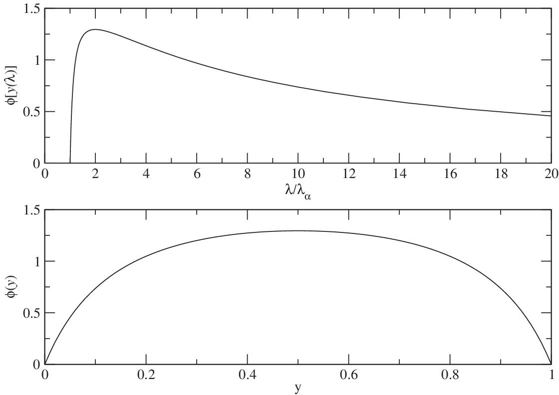
0.14 Results
Each of the line distortions is shown separately in Fig. 6 and summed for each species in Fig. 7. The shape of the lines from H i, He i and He ii are fairly similar. There are two distinct peaks to the 2p–1s emission lines. We refer to the one located at longer wavelength as the ‘pre-recombination peak’, since the corresponding atoms had hardly started to recombine during that time. The physics of the formation of this peak will be discussed in detail in section 0.14.1. The second (shorter wavelength) peak is the main recombination peak, which was formed when the atoms recombined. While the longer wavelength peak actually contains almost an order of magnitude more flux, it makes a much lower relative distortion to the CMB. The ratio of the total distortion to the CMB intensity is shown in Fig. 8. It is for the main recombination peak, but for the pre-recombination peak.
In Fig. 7, we plot the lines from H i and He i together with the CMB and an estimate of the CIB. We can see that the lines which make the most significant distortion to the CMB are the Ly line and the 21p–11s line of He i, and that these lines form a non-trivial shape for the overall distortion. The sum of all the spectral lines and the CMB is shown in Fig. 7. Note that these lines will also exist in the presence of the CIB – but the shape of this background is currently quite poorly determined [17, 21].
We now discuss details of the physics behind the shapes of each of the main recombination lines.


0.14.1 Lines from the recombination of hydrogen
During recombination, the Lyman lines are optically thick, which means that nearly all photons emitted from the transition to are instantly reabsorbed. However, some of the emitted photons redshift out of the line due to the expansion of the Universe and this makes the Ly transition one of the possible ways for electrons to cascade down to the ground state. The other path for electrons going from to is the two-photon transition between 2s and 1s. Fig. 9 shows the net photon emission rate of the Ly and two-photon transitions as a function of redshift for the standard CDM model. The two-photon rate dominates at low redshift, where the bulk of the recombinations occur. This means that there are more photons emitted through the two-photon emission process (54% of the total number of photons created during recombination of H) than through the Ly redshifting process. This conclusion agrees with Zeldovich et al. (1968) [59] – although of course the balance depends on the cosmological parameters (see [51]) and for today’s best fit cosmology the two processes are almost equal. Despite this fact, the overall strength of the two-photon emission lines are weaker because the photons are not produced with a single frequency, but with a wide spectrum ranging from 0 to . The location of the two-photon peak (see Fig. 6) is also somewhat unexpected, since it is almost at the same wavelength as the Ly recombination peak, rather than at twice the wavelength. The reason for this will be discussed in the following subsection.
We should also note that the tiny dip in our curves for the long-wavelength tail of the pre-recombination peak (see Fig. 6) is due to a numerical error, when the number density of the ground state is very small. This can also be seen in the pre-recombination peak for Heii.
The pre-recombination emission peak
The highest Ly peak (shown in Fig. 6) is formed before the recombination of H has already started, approximately at . During that time the emission of Ly photons is controlled by the bound-bound Ly rate from (i.e. the term in equation (33)) and the photo-ionization rate (). From Fig. 10, we can see that at early times the bound-bound Ly rate is larger than the photo-ionization rate. This indicates that when an electron recombines to the state, it is more likely to go down to the ground state by emission of a Ly photon than to get ionized. The excess Ly alpha photons are not reabsorbed by ground state H, but are redshifted out of the absorption frequency due to the expansion of the Universe; they escape freely and form the pre-recombination emission line. Note that there is very little net recombination of H, since the huge reservoir of eV CMB photons keeps photo-ionizing the ground state H atoms (see Fig. 16).


We now turn to a more detailed explanation of the pre-recombination emission peak. The bound-bound Ly rate from is initially approximately constant, as it is dominated by the spontaneous de-excitation rate (the term in equation (45)). At the same time the photo-ionization rate is always decreasing as redshift decreases, since the number of high energy photons keeps decreasing with the expansion of the Universe. Therefore, with a constant bound-bound Ly rate and the decreasing photo-ionization rate, the emission of Ly photons rises. The peak of this pre-recombination line of H occurs at around = 3000, by which time only a very tiny amount of ground state H atoms have formed (, see Fig. 10). These ground state H atoms build up until they can reabsorb the Ly photons and this lowers the bound-bound Ly rate. The decrease of the bound-bound Ly rate is represented in the Sobolev escape probability in equation (36). At high redshift, is 1 and there is no trapping of Ly photons. When H starts to recombine, the optical depth increases and the Ly photons can be reabsorbed by even very small amounts of neutral H. For , we can approximate and . Because of the increase of the number density of the ground state and the decrease of , the pre-recombination line decreases. One can therefore think of the ‘pre-recombination peak’ as arising from direct Ly transitions, before enough neutral H has built up to make the Universe optically thick for Lyman photons. This process occurs because the spontaneous emission rate ( term) is faster than the photo-ionization rate for ; it increases as the Universe expands, due to the weakening CMB blackbody radiation, and is quenched as the fraction of atoms in the = 1 level grows. The shorter wavelength peak, on the other hand, comes from the process of redshifting out of the Ly line during the bulk of the recombination epoch.
By using the recfast program [50], we can generate the main Ly recombination peak and also the two-photon emission spectrum, by simply adding a few lines into the code. However, the pre-recombination peak cannot be generated from recfast, since there the rate of change of the number density of the first excited state is assumed to be negligible and is related to via thermal equilibrium. Moreover, in the effective 3-level formalism, the Ly line is assumed to be optically thick throughout the whole recombination process of H (in order to reduce the calculation into a single ODE), which is not valid at the beginning of the recombination process. Hence, one needs to follow the rate equations of both states (i.e. = 1 and = 2) to generate the full Ly emission spectrum. The pre-recombination peak of H was mentioned and plotted in the earlier work of Dell’Antonio & Rybicki (1993) [5] as well, although they did not describe it in any detail.
Another way to understand the line formation mechanism is to ask how many photons are made in each process per atom. We find that for the main Ly peak there are approximately 0.47 photons per hydrogen atom (in the standard cosmology). During the recombination epoch, net photons for the to transitions are only made when atoms terminate at the ground state. Hence we expect exactly one = 2 to = 1 photon for each atom, split between the Ly redshifting and 2-photon processes (and the latter splits the energy into two photons, so there are 1.06 of these photons per atom). For the ‘pre-recombination peak’, on the other hand, the atoms give a Ly photon when they reach , but they then absorb a CMB continuum photon to get back to higher or become ionized. The number of times an atom cycles through this process depends on the ratio of the relevant rates. If we take the rate per unit volume from Fig. 9 and divide by the number density of hydrogen atoms at then we get a rate which is about an order of magnitude larger than the Hubble parameter at that time. Hence we expect about 10 ‘pre-recombination peak’ photons per hydrogen atom. A numerical calculation gives the more precise value of 8.11.
The two-photon emission lines
Surprisingly, the location of the peak of the line intensity of the 2s–1s transition is almost the same as that of the Ly transition, as shown in Fig. 6, while one might have expected it to differ by a factor of 2. In order to understand this effect, we rewrite the equation (46) in the following way:
| (47) |
where , and
| (48) |
with
Equation (48) gives the redshifted flux (measured now at = 0) of a single frequency coming from redshift and corresponding to the redshifted frequency .
We first calculate the line intensity of the two-photon emission with a simple approximation: a delta function spectrum , where is the frequency corresponding to the peak of the two-photon emission spectrum . Fig. 11 shows the intensity spectrum of two-photon emission using a delta frequency spectrum compared with the two-photon emission using the correct spectrum . We can see that there is a significant shift in the line centre compared with the -function case. Where does this shift come from?

We know that the frequencies of emitted photons are within the range of 0 to at the time of emission. For a fixed redshifted frequency now, we can calculate the range of emission redshifts contributing to (referred to as the ‘contribution period’ from now on), which is represented by or . In Fig. 12, we show the spectral distribution as a function of redshift for specific values of . For example, if we take , then photons emitted between (i.e. ) and () will give contributions to . The smaller the redshifted frequency , the wider the contribution period. We might expect that the line intensity of this two-photon emission will be larger if the contribution period is longer, as there are more redshifted photons propagating from earlier times. However, this is not the case, because the rate of two-photon emission also varies with time, and is sharply peaked at 1300–1400. Hence is also sharply peaked at 1300–1400. In Fig. 12, the redshifted flux integrand and the emission spectrum are plotted on the same redshift scale. For (lowest panel), we can see that the contribution period covers a redshift range when and are small in value. The contribution period widens with decreasing and covers more of the redshift range when two-photon emission was high. Therefore, the flux is expected to increase with decreasing until the contribution period extends to the redshifts at which the two-photon emission peaks. As gets even smaller (e.g. Hz), then the contribution period becomes larger than the redshift range for two-photon emission and hence only lower energy photons can be redshifted to that redshifted frequency. As a result, the flux starts to decrease, and so we have a peak. The flux peaks at when we use the -function approximation. However, from Fig. 12, we can see that the contribution period for is much greater than that of the two-photon emission period, and therefore this is not the location of peak. Based on the argument presented above, we expect the peak to be at around , or m.

The basic mathematical point is that is extremely poorly represented by a -function. Since the spectrum is quite broad, it can be better approximated as a uniform distribution than as a -function. Another crude approximation would be to assume a flat spectrum for in Fig. 5. Fig. 11 compares the intensity found using the correct form for with the -function and flat spectrum approximations. This shows that the flat spectrum gives qualitatively the same results as the correct form of the spectrum, and that the peak occurs fairly close to that of Ly, but is much broader. The same general arguments apply to the two-photon lines of He i and He ii (as we discuss in Section 3.3.2).
Dependence of and
The largest distortion on the CMB is from the shorter wavelength recombination peak of the hydrogen Ly line (see Fig. 8). It may therefore be useful estimate the peak of this line’s intensity as a function of the cosmological parameters. The relevant parameters are the matter density () and the baryon density (). This is because affects the expansion rate, while is related to the number density of hydrogen. No other combinations of cosmological parameters have a significant impact on the physics of recombination.
We can crudely understand the scalings of these parameters through the following argument. Regardless of the escape probability , the remaining part of the rate is roughly proportional to . The escape probability can be approximated as 1 at the beginning of recombination and during the bulk of the recombination process (with . Note that . Therefore,
| (49) |
and thus
| (50) |
From this rough scaling argument, we may expect that the dependence of the peak of the Ly line is an approximate power law with index between and 0, while for the corresponding power-law index is expected to lie between 0 and 1. The dependence of is actually more complicated when one allows for a wider range of values (see [5]). The above estimation just gives a rough physical idea of the power of the dependence.
A more complete numerical estimate of the peak of the recombination Ly distortion is:
| (51) |
where we have normalized to the parameters of the currently favoured cosmological model. The peak occurs at
| (52) |
for all reasonable variants of the standard cosmology.
0.14.2 Lines from the recombination of helium (He i and He ii)
We compute the recombination of He ii and He i in the same way as for hydrogen. For the two-electron atom He i, we ignore all the forbidden transitions between singlet and triplet states due to the low population of the triplet states (see [50, 51]). The p–11s transitions of He i are optically thick, the same situation as for H. This makes the electrons take longer to reach the ground state and causes the recombination of He i to be slower than Saha equilibrium. However, unlike for H, and despite the optically thick p–11s transition line, the p–11s rate dominates, as shown in Fig. 13. For He ii, due to the fast two-photon transition rate (see Fig. 14), there is no ‘bottleneck’ at the level in the recombination process. Hence He ii recombination can be well approximated by using the Saha equilibrium formula [51].

We can see the effect of the above differences in recombination history on the lines: the width of the recombination peak of both H and He i is larger than that of He ii. Overall, the spectral lines of He ii are of much lower amplitude than those of H (see Fig. 6) with the distortion to the CMB about an order of magnitude smaller.
The peaks of the line distortions from H and He ii are located at nearly the same wavelengths. For hydrogenic ions the 1s–2p energy (and all the others) scales as , where is the atomic number. Hence for He ii recombination takes place at rather than the for hydrogen. Hence the line distortion from the 2p–1s transition of He ii redshifts down to about m, just like Ly.
The two-photon frequency spectrum of He ii is the same as for H, since they are both single-electron atoms [56]. However, it is complicated to calculate the two-photon frequency spectrum of He i very accurately, since there is no exact wave-function for the state of the atom. Drake et al. (1969) [8] used a variational method to calculate the two-photon frequency spectrum of He i with values given up to 3 significant figures. Drake (1986) [9] presented another calculation, giving one more digit of precision, and making the spectrum smoother, as shown in Fig. 15. These two calculations differ by only about 1%, which makes negligible change to the two-photon He i spectral line.
All of the H and He lines (for = 2 to = 1) are presented in Fig. 6 and the sum is shown as a fractional distortion to the CMB spectrum in Fig. 8. We find that in the standard cosmological model, for He i recombination, there are about 0.67 photons created per helium atom in the ‘main’ p–s peak, 0.70 per helium atom in the ‘pre-recombination peak’, and 0.66 in the two-photon process. The numbers for He ii recombination are 0.62, 0.76 and 6.85 for these three processes, respectively.


0.15 Discussion
0.15.1 Modifications in the recombination calculation
There are several possible improvements that we could make to the line distortion calculation. However, as we will discuss below, we do not believe that any of them will make a substantial difference to the amplitudes of the lines.
In order to calculate the distortion lines to higher accuracy, we should use the multi-level model without any thermal equilibrium assumption among the bound states. And we also need to take into account the secondary spectral distortion in the radiation field, i.e. we cannot approximate the background radiation field as a perfect blackbody spectrum. This means, for example, that the extra photons from the recombination of He i may redshift into an energy range that can photo-ionize H( = 1) [5, 51]. We can assess how significant this effect might be by considering the ratio of the number of CMB background photons with energy larger than , , to the number of baryons, , at different redshifts (see Fig. 16).
Roughly speaking, the recombination of H occurs at the redshift when is about equal to 1. This is because at lower redshifts there are not enough high energy background photons to photo-ionize or excite electrons from the ground state to the upper states (even to = 2), while at higher redshift, when such transitions are possible, there are huge numbers of photons able to ionize the level. The solid line in Fig. 16 shows the effect of the helium line distortions on the number of high energy photons (above Ly) per baryon. The amount of extra distortion photons with redshifted energy larger than coming from the recombination of Hei is only about 1 per cent of the number of hydrogen atoms. Their effect is therefore expected to be negligibly small for . We neglect the effect of the helium recombination photons on the hydrogen line distortion, since it is clearly going to make a small correction (at much less than the 10 per cent level).
As well as this particular approximation, there have been some other recent studies which have suggested that it may be necessary to make minor modifications to the recombination calculations presented in Seager et al. (1999, 2000) [50, 51]. Although these proposed modifications would give only small changes to the recombination calculation, it is possible that they could have much more significant effects on the line amplitudes and shapes. Recent papers have described 3 separate potential effects.
In the effective three-level model, Leung et al. (2004) [30] argued that the adiabatic index of the matter should change during the recombination process, as the ionized gas becomes neutral, giving slight differences in the recombination history. Dubrovich & Grachev (2005) [13] have claimed that the two-photon rate between the lowest triplet state and the ground state and that between the upper singlet states and the ground state should not be ignored in the recombination of Hei. And Chluba & Sunyaev (2005) [4] suggested that one should also include stimulated emission from the 2s state of H, due to the low frequency photons in the CMB blackbody spectrum. Even if all of these effects are entirely completely correct, we find that the change to the amplitude of the main spectral distortion is much less than 10%. We therefore leave the detailed discussion of these and other possible modifications to a future work.

0.15.2 Possibility of detection
There is no avoiding the fact that detecting these CMB spectral distortions will be difficult. There are three main challenges to overcome: (1) achieving the required raw sensitivity; (2) removing the Galactic foreground emission; and (3) distinguishing the signal from the CIB.
Let us start with the first point. We can estimate the raw sensitivity achievable in existing or planned experiments (even although these instruments have not been designed for measuring the line distortion). Since the relevant wavelength range is essentially impossible to observe from the ground, it will be necessary to go into space, or at least to a balloon-based mission. One existing experiment with sensitivity at relevant wavelengths is BLAST [6] which has an array of bolometers operating at m on a balloon payload. The estimated sensitivity is mJy in s, for a 30 arcsec FWHM beam, which corresponds to . Comparing with equation (51) for the peak intensity, it would take such detectors running for a year to detect the line distortion. The SPIRE instrument on Herschel will have a similar bolometer array, but with better beamsize. The estimated sensitivity of mJy at in 1 hour for a 17.4 arcsec FWHM beamsize [20] corresponds to per detector for the sensitivity in second. So detection of the line would still require such detectors operating for a year.
These experiments are limited by thermal emission from the instrument itself, and so a significant advance would come from cooling the telescope. This is one of the main design goals of the proposed SAFIR [29] and SPICA [36] missions. One can imagine improvements of a factor for far-IR observations with a cooled mirror. This would put us in the regime where arrays of detectors (of a size currently being manufactured for sub-mm instruments) could achieve the desired sensitivity.
One could imagine an experiment designed to have enough spectroscopic resolution to track the shape of the expected line distortion. The minimum requirement here is rather modest, with only in at least 3 bands. An important issue will be calibration among the different wavelengths, so that the non-thermal shape can be confidently measured. To overcome this, one might consider the use of direct spectroscopic techniques rather than filtered or frequency-sensitive bolometers.
Another way of quoting the required sensitivity is to say that any experiment which measures the recombination line distortion would have to measure the CIB spectrum with a precision of about 1 part in , which is obviously a significant improvement over what has been currently achieved. A detection of the line distortion might therefore naturally come out of an extremely precise measurement of the CIB spectrum, which would also constrain other high frequency distortions to the CMB spectrum.
Some of the design issues involved in such an experiment are discussed by Fixsen & Mather (2002) [18]. They describe a future experiment for measuring deviations of the CMB spectrum from a perfect blackbody form, with an accuracy and precision of 1 part in . This could provide upper limits on Bose-Einstein distortion and Compton distortion parameters at the level (the current upper limits for and are and , respectively; [16]). The frequency coverage they discuss is 2–120 (about 80–5,000m), which extends to much longer wavelengths than necessary for measuring the line distortion. The beam-size would be large, similar to FIRAS, but the sensitivity achieved could easily be 100 times better. An experiment meant for detecting the line distortion would have to be another couple of orders of magnitude more sensitive still.
Turning to the second of the major challenges, it will be necessary to detect this line in the presence of the strong emission from our Galaxy. At m the Galactic Plane can be as bright as which is about a billion times brighter than the signal we are looking for! Of course the brightness falls dramatically as one moves away from the Plane, but the only way to confidently avoid the Galactic foreground is to measure it and remove it. So any experiment designed to detect the line distortion will need to cover some significant part of the sky, so that it will be possible to extrapolate to the cosmological background signal. The spectrum of the foreground emission is likely to be smoother than that of the line distortion, and it may be possible to use this fact to effectively remove it. However, it seems reasonable to imagine that the most efficient separation of the signals will involve a mixture of spatial and spectral information, as is done for CMB data (see, for example, [38]).
In the language of spherical harmonics, the signal we are searching for is a monopole, with a dipole at the level and smaller angular scale fluctuations of even lower amplitude. Hence we would expect to be extrapolating the Galactic foreground signals so that we can measure the overall DC level of the sky. This is made much more difficult by the presence of the CIB, which is also basically a monopole signal. Hence spatial information cannot be used to separate the line distortion from the CIB. The measurement of the line distortion is therefore made much more difficult by the unfortunate fact that the CIB is several orders of magnitude brighter – this is the third of the challenges in measuring the recombination lines.
The shape of the CIB spectrum is currently not very well characterised. It was detected using data from the DIRBE and FIRAS experiments on the COBE satellite. Estimates for the background () are: at m [35]; at m [27]; at m [21, 26]; and at m [21, 26]; In each case the detections are only at the 3– level, and the precise values vary between different prescriptions for data analysis (see also [15, 22, 48]). The short wavelength distortion of the CMB, interpretted as a measurement of the CIB [43] can be fit with a modified blackbody with temperature K and emissivity index 0.64 (although there is degeneracy between these parameters), which we plotted in Fig. 7.
The CIB is thus believed to peak somewhere around m, which is just about where we are expecting the recombination line distortion. The accuracy with which the CIB spectrum is known will have to improve by about 5 orders of magnitude before the distortion will be detectable. Fortunately the spectral shape is expected to be significantly narrower than that of the CIB – the line widths are similar to the for the last scattering surface thickness, as opposed to for a modified blackbody shape (potentially even wider than this, given that the sources of the CIB come from a range of redshift ).
One issue, however, is how smooth the CIB will be at the level of detail with which it will need to be probed. It may be that emission lines, absorption features, etc. could result in sufficiently narrow structure to obscure the recombination features. We are saved by 2 effects here: firstly the CIB averaged over a large solid angle patch is the sum of countless galaxies, and hence the individual spectral features will be smeared out; and secondly, the far-IR spectral energy distributions of known galaxies do not seem to contain strong features of the sort which might mimic the recombination distortion (see, for example, [28]). As we learn more about the detailed far-IR spectra of individual galaxies we will have a better idea of whether this places a fundamental limit on our ability to detect the recombination lines.
Overall it would appear that the line distortion should be detectable in principle, but will be quite challenging in practice.
0.16 Conclusion
We have studied the spectral distortion to the CMB due to the Ly and 2s–1s two-photon transition of H i and the corresponding lines of He i and He ii. Together these lines give a quite non-trivial shape to the overall distortion. The strength and shape of the line distortions are very sensitive to the details of the recombination processes in the atoms. Although the amplitude of the spectral line is much smaller than the Cosmic Infrared Background, the raw precision required is within the grasp of current technology, and one can imagine designing an experiment to measure the non-trivial line shape which we have calculated. The basic detection of the existence of this spectral distortion would provide incontrovertible proof that the Universe was once a hot plasma and its amplitude would give direct constraints on physics at the recombination epoch.
0.17 Remarks
Since this work was published, there have been other studies calculating the same spectral distortions with different approach in a different independent numerical code [45, 46]. Rubiño-Martín et al. (2006) [45] pointed out a correction in the treatment of the two-photon spectrum, and found no pre-recombination peak in the H Ly line distortion, in contradiction to the results of this chapter. As an addition to our published study, we now discuss these two issues.
Normalization of the two-photon spectrum
In our calculation of the two-photon line distortion, the emission spectrum is normalized to 1 (see Figure 5 and Equation (3.22)). However, the two-photon spectrum should be normalized to 2 (as pointed out by [45]) because there are two photons emitted in each electron transition from the 2s state to the ground state. Due to this correction, the intensity of the two-photon line distortion presented before should be doubled. For H i, since the amplitude of the distortion from Ly emission is about 10 times larger than the two-photon contribution, the overall shape and the peak location of the line spectrum remain almost the same as before. The same correction should be made for the helium line distortion spectrum as well, and again the effect or the overall distortion from He is small.
The pre-recombination peak
Rubiño-Martín et al. (2006) [45] performed an independent calculation of the spectral line distortions from H i recombination with a multi-level atom model. The authors adopted the same procedure described in Seager et al. (2000) [51] but considered separate -states within each -shell of H i with no thermal equilibrium assumption. In this Chapter, we obtained a pre-recombination peak using a 3-level atom model also based on the recombination model given by Seager et al. (2000) [51]. In contrast, Rubiño-Martín et al. (2006) [45] found no pre-recombination peak in their calculation.
As with earlier work [5], our pre-recombination peak was only found from numerical calculation and no explicit theoretical argument for the formation of this peak was given. We can consider the calculation a different way in order to understand the underlying physics. Since the population of the hydrogen atom states is well described by the Boltzmann equations before recombination (say 1700 for H i; see for example [51]), we now present an analytical estimate of the H i pre-recombination peak under the local thermal equilibrium assumption in a 3-level atom model.
The pre-recombination peak was previously found in the calculation of the H i Ly emission line, and also for the corresponding He i and He ii emission lines. Here we only discuss the case of H i, since the physics is basically the same for other species within the standard recombination model [51]. Since the spectrum of the photon emission in this transition is narrowly peaked at the Ly frequency, the distortion shape is mainly controlled by the net Ly emission rate (see Equation (43)). From Equation (33), the net Ly rate can be rewritten as
| (53) |
Here we approximate . We can also write the net 2s–1s two-photon rate as
| (54) |
by assuming that the 2p and 2s states are in thermal equilibrium. From the above equations, we can see that these two rates are controlled by the same difference, i.e. the difference between the ratio and its local thermal equilibrium value from the Boltzmann factor.
Rubiño-Martín et al. (2006) [45] argued that is equal to zero at because the states are in thermal equilibrium. This is not entirely true, since the expanding Universe is a fundamentally out-of-equilibrium system; we will show that is non-zero (although the rate is very low) even if the population of the states in H i is well approximated by the Boltzmann distribution at each instant of time during the pre-recombination period. From the Saha equation, we have
| (55) |
where is the frequency of the energy difference between the th state and the continuum. We can take Equation (55) for = 1 (1s, the ground state), differentiate with respect to and substitute into Equation (3.1), giving
| (56) |
The right-hand side of the above equation is dominated by the first two terms, since
| (57) |
and
| (58) |
before the recombination of H i ( 1800). This makes the sum of the two rates larger than zero and implies that there are net recombinations to the ground state even in the case that the number density of each state closely follows the thermal equilibrium distribution. Physically, the non-zero net recombination rate of H i is due to the decreasing number of high-energy photons in the expanding Universe. And as we know from Equation (3.31) and (3.32),
| (59) |
Before the H i recombination ( 1800 say), the net Ly rate dominates, because the neutral hydrogen abundance is very low and the escape probability is very close to 1. Therefore, we can ignore in Equation (56) and we have
| (60) |
In Figure 17, the approximate rate is plotted along with the previous result from the numerical recombination code. We can see that matches the numerical rate very well when the hydrogen is about to recombine at =1800–2000. These two rates are expected to depart at when the ground state goes out of thermal equilibrium with the higher excited states due to the bottleneck at the first excited state. On the other hand, we expect the thermal equilibrium assumption to be valid at even higher redshifts ( 2000). Under this assumption, we find no significant emission before recombination and therefore, there is no pre-recombination peak. Why does this result contradict with what we found in the numerical calculation?

In fact we found that the pre-recombination peak that we presented before arose due to a systematic error in the ODE (ordinary differential equation) solver. Any ODE solver allows us to find a numerical approximation to an exact (or real) solution of the equations to within some error. We usually want the relative error to be small, and this is controlled by setting the required accuracy as an input parameter in the solver. In our case, the relative error of the number density is ( and are the real and numerical values of , respectively).
Now consider the effect of this error on the net rates. The net rates are strongly controlled by the deviation of the ratio from its Boltzmann value. Note that
| (61) | |||||
where , should be the same order of magnitude as the uncertainty in (i.e. ). In the above equation, the first bracket accounts for how much the first excited state and the ground state are out of equilibrium and this gives us the actual net Ly rate. The second term is the error in the Ly rate due to the numerical errors in the number densities. Somewhat surprisingly, it is directly proportional to the actual value of , which increases with . In the pre-recombination epoch, we can approximate using Boltzmann equations in order to calculate the error of the rate. For comparison, we use Equation (3.31) to obtain the estimate
| (62) |
In Fig. 18, we separately plot the two terms in Equation (61) as well as from the numerical code. The estimated numerical error dominates at and it matches well with the curve if we take , which is even smaller than the required accuracy in the ODE solver. This error term explains why there is an anomalous increasing trend of at high , while we expect the difference in the ratio to get smaller with increasing due to the tight thermal equilibrium relation between the states. This estimated numerical error is directly proportional to and decreases with decreasing . On the other hand, is getting larger and larger as the recombination of hydrogen begins. So at , takes over. This explains why the and values agree with each other only in the range of 1600–2000. Overall, the pre-recombination peak that we found earlier seems to have beem caused by a systematic error. This should serve as a warning for blindly accepting numerical result.
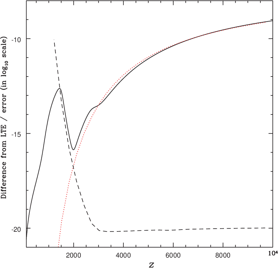
Physically, any possible pre-recombination peak or extra emission through the H i Ly transition would require channels for electrons in the ground state to get back to higher excited states or the continuum, since there is almost no net neutral hydrogen H i formed due to these processes. In the three-level atom model, no such path exists since all the transitions to and from the ground state are connected with the first excited state ( = 2). We have also investigated this problem in a multi-level atom model based on the paper of Seager et al. (2000) [51], and still find no such net excitation to the higher excited states. From this physical reasoning and the previous analysis of numerical errors, the pre-recombination peak we found in the standard recombination calculation therefore appears to have been a false signal.
On the other hand, additional radiative processes not considered in the standard recombination model of Seager et al. (2000) [51] provide the channels necessary for a pre-recombination peak. In the recent studies which include addditional continuum opacity of H i in the He i recombination [25, 55] evolution, the extra high energy distortion photons from He i recombination can excite the electrons in the ground state for H i atom before the recombination of H i at = 1600 – 2200. This allows for direct ionization from the ground state, and a narrow ‘pre-recombination peak’ in the H i Ly line is formed at 1870 (see Figure 9 in [46]). This effect is, however, much smaller than the previous false signal. The amplitude of this pre-recombination peak is about an order of magnitude smaller than the main peak of the H i Ly line formed during H i recombination.
To conclude, the pre-recombination peaks found in our previous studies [5, 57] seem to have been false signals coming from a systematic error in the numerical code (for both H and He). By including the direct ionization from the ground state of H i due to the distortion photons from He i recombination, we can find a pre-recombination peak in the H i Ly line, but with a much reduced amplitude.
0.18 References
References
- [1] Boschan P., Biltzinger P. 1998, Astronomy and Astrophysics, 336, 1
- [2] Burdyuzha V. V., Chekmezov A. N. 1994, Astronomicheskii Zhurnal, 71, 341
- [3] Burgin M. S. 2003, Astronomicheskii Zhurnal, 80, 9, 771; English translation, 2003, Astronomy Reports, 47, 9, 709
- [4] Chluba J., Sunyaev R. A. 2006, Astronomy and Astrophysics, 446, 39
- [5] Dell’Antonio I. P., Rybicki G. B. 1993, in ASP Conference Series 51, Observational Cosmology, ed. G.Chincarini et al. (San Francisco:ASP), 548
- [6] Devlin M. J. et al. 2004, Millimeter and Submillimeter Detectors for Astronomy II. Edited by Jonas Zmuidzinas, Wayne S. Holland and Stafford Withington Proceedings of the SPIE, 5498, 42
- [7] Derevianko A., Johnson W. R. 1997, Physical Review A, 56, 1288
- [8] Drake G. W. F., Victor G. A., Dalgamrno A. 1969, Physical Review, 180, 25
- [9] Drake G. W. F. 1986, Physical Review A, 34, 2871
- [10] Dubrovich V. K. 1975, Soviet Astronomy Letters, 1, 196
- [11] Dubrovich V. K., Stolyarov V. A. 1995, Astronomy and Astrophysics, 302, 635
- [12] Dubrovich V. K., Stolyarov V. A. 1997, Astronomy Letters, 23, 565
- [13] Dubrovich V. K., Grachev S. I. 2005, Astronomy Letters, 31, 359
- [14] Fahr H. J., Loch R. 1991, Astronomy and Astrophysics, 246, 1
- [15] Finkbeiner D. P., Davis M., Schlegel D. J. 2000, Astrophysical Journal, 544, 81
- [16] Fixsen D. J., Cheng E. S., Gales J. M., Mather J. C., Shafer R. A., Wright E. L. 1996, Astrophysical Journal, 473, 576
- [17] Fixsen D. J., Dwek E., Mather J. C., Bennett C. L., Shafer R. A. 1998, Astrophysical Journal, 508, 123
- [18] Fixsen D. J., Mather J. C. 2002, Astrophysical Journal, 581, 817
- [19] Goldman S. P. 1989, Physical Review A, 40, 1185
- [20] Griffin M. J., Swinyard B. M., Vigroux L. 2001, The Promise of the Herschel Space Observatory, ed. G.L. Pilbratt, J. Cernicharo, A.M. Heras, T. Prusti & R. Harris, ESA Special Publication, 460, 37
- [21] Hauser M. G. et al. 1998, Astrophysical Journal, 508, 25
- [22] Hauser M. G., Dwek E. 2001, Annual Review of Astronomy and Astrophysics, 39, 249
- [23] Hummer D. G. 1994, Monthly Notices of the Royal Astronomical Society, 268,109
- [24] Kholupenko E. E., Ivanchik A. V., Varshalovich D. A. 2005, Gravitation and Cosmology, 11, 161
- [25] Kholupenko E. E., Ivanchik A. V., Varshalovich D. A. 2007, Monthly Notices of the Royal Astronomical Society, L42
- [26] Lagache G., Abergel A., Boulanger F., Désert F. X., Puget J.-L. 1999, Astronomy and Astrophysics, 344, 322
- [27] Lagache G., Haffner L. M., Reynolds R. J., Tufte S. L. 2000, Astronomy and Astrophysics, 354, 247
- [28] Lagache G., Puget J.-L., Dole H. 2005, Annual Review of Astronomy & Astrophysics, 43, 727
- [29] Leisawitz D. 2004, Advances in Space Research, 34, 631
- [30] Leung P. K., Chan C. W., Chu M. C. 2004, Monthly Notices of the Royal Astronomical Society, 349, 2, 632
- [31] Lipeles M., Novick R., Tolk N., 1965, Physics Review Letter, 15, 690
- [32] Lyubarsky Y. E., Sunyaev R. A. 1983, Astronomy and Astrophysics, 123, 171
- [33] Martinis M., Stojic M. 2000, Fizika A, 9, 115
- [34] Mather J. C., Fixsen D. J., Shafer R. A., Mosier C., Wilkinson D. T. 1999, Astrophysical Journal, 512, 511
- [35] Miville-Deschênes M.-A., Lagache G., Puget J.-L. 2002 Astronomy and Astrophysics, 393, 749
- [36] Nakagawa T. et al, 2004, Advances in Space Research, 34, 3, 645
- [37] Padmanabhan T. 1993, Structure Formation in the Universe, Cambridge Univ. Press, Cambridge, UK
- [38] Patanchon G., Cardoso J.-F., Delabrouille J., Vielva P. 2004, submitted to Monthly Notices of the Royal Astronomical Society, preprint(astro-ph/0410280)
- [39] Peebles P. J. E. 1968, Astrophysical Journal, 153, 1
- [40] Peebles P. J. E., Seager S., Hu W. 2000, Astrophysical Journal, 539, L1
- [41] Pequignot D., Petitjean P., Boisson C. 1991, Astronomy and Astrophysics, 251, 680
- [42] Press W. H., Flannery B. P., Teukolsky S. A., Vetterling W. T. 1992, Numerical Recipes in C: The Art of Scientific Computing, Cambridge Univ. Press, Cambridge, UK
- [43] Puget J.-L. et al. 1996, Astronomy and Astrophysics, 308, L5
- [44] Rubiño-Martí, J. A., Hernández-Monteagudo C., Sunyaev R. A. 2005, Astronomy and Astrophysics, 438, 461
- [45] Rubiño-Martín J. A., Chluba J., Sunyaev R. A. 2006, Monthly Notices of the Royal Astronomical Society, 371, 1939
- [46] Rubiño-Martín J. A., Chluba J., Sunyaev R. A. 2007, ArXiv e-prints, arXiv:0711.0594
- [47] Santos J. P., Parente F., Indelicato P. 1998, The European Physical Journal D, 3, 43
- [48] Schlegel D. J., Finkbeiner D. P., Davis M. 1998, Astrophysical Journal, 500, 525
- [49] Scott D., Smoot G. 2004, The Review of Particle Physics, S. Eidelman et al., Physics Letters B., 592, 1
- [50] Seager S., Sasselov D. D., Scott D. 1999, Astrophysical Journal, 523, L1
- [51] Seager S., Sasselov D. D., Scott D. 2000, Astrophysical Journal Supplement, 128, 407
- [52] Spergel D. N. et al. 2003 Astrophysical Journal Supplement, 148, 175
- [53] Spitzer L., Greenstein J. L. Jr., 1951, Astrophysical Journal, 114, 407
- [54] Switzer E. R., Hirata C. M. 2005, Physical Review D, 72, 083002
- [55] Switzer E. R., Hirata C. M. 2008, Physical Review D, 77, 083006
- [56] Tung J. H., Ye X. M., Salamo G. J., Chan F. T. 1984, Physical Review A, 30, 1175
- [57] Wong W. Y., Seager S., Scott D. 2006, Monthly Notices of the Royal Astronomical Society, 367, 1666
- [58] Wright E. L. 2004, New Astronomy Reviews, 48, 465
- [59] Zeldovich Y. B., Kurt V. G., Syunyaev R. A. 1968, Zhurnal Eksperimental noi i Teoreticheskoi Fiziki, 55, 278: English translation: 1969, Soviet Physics-JETP, 28,146
Chapter 0 Forbidden transitions33 3 A version of this chapter has been published: Wong W. Y. and Scott D. (2007) ‘The effect of forbidden transitions on cosmological hydrogen and helium recombination’, Monthly Notices of the Royal Astronomical Society, 375, 1441–1448.
0.19 Introduction
The release of the third year data from the Wilkinson Microwave Anisotropy Probe (WMAP) has further improved the precision with which we can constrain the cosmological parameters from the shape of the Cosmic Microwave Background (CMB) anisotropies [28]. The Planck satellite, scheduled for launch in 2008 [20], will provide even higher precision values and data down to smaller angular scales (). Higher precision in the observations requires increased accurarcy from the theoretical calculations, in order for the correct cosmological parameters to be extracted. It now seems crucial to obtain the s down to at least the 1 percent level over a wide range of .
cmbfast [27] is the most commonly used Boltzmann code for calculating the s, and it gives consistent results with other independent codes (see [26] and references therein). The dominant uncertainty in obtaining accurate s comes from details in the physics of recombination, for example, the ‘fudge factor’ in the recfast routine [24, 25]. Calculations of cosmological recombination were first published by Peebles (1968) [19] and Zeldovich et al. (1968) [35]. Seager et al. (2000) [25] presented the most detailed multi-level calculation and introduced a fudge factor to reproduce the results within an effective three-level atom model. Although the multi-level calculation already gives reasonable accuracy, the required level of accuracy continues to increase, so that today any effect which is 1 per cent over a range of multipoles is potentially significant. Several modifications have been recently suggested to give per cent level changes in the ionization fraction and/or the s (see Section 4.4 for details). Most of these modifications have been calculated only with an effective three-level code, and so the results may be different in the multi-level calculation, since there is no thermal equilibrium assumed between the upper states. Here we want to focus on one of these modifications, namely the extra forbidden transitions proposed by Dubrovich & Grachev (2005) [7], which we study using a multi-level code.
In the standard calculations of recombination, one considers all the resonant transitions, but only one forbidden transition, which is the 2S–1S two-photon transition, and this can be included for both H and He. Dubrovich & Grachev (2005) [7] suggested that one should also include the two-photon transitions from higher excited S and D states to the ground state for H and He i, and also the spin-forbidden transition between the triplet P1 and singlet ground state S0 for He i. They showed that the recombination of both H i and He i sped up in the three-level atom model. The suggested level of change is large enough to bias the determination of the cosmological parameters [16].
In this chapter we try to investigate the effect of the extra forbidden transitions suggested by Dubrovich & Grachev (2005) [7] in the multi-level atom model without assuming thermal equilibrium among the higher excited states. The outline of this chatper is as follows. In Section 0.20 we will describe details of the rate equations in our numerical model. In Section 0.21 we will present results on the ionization fraction and the anisotropies , and assess the importance of the addition of the forbidden transitions. Other possible improvements of the recombination calculation will be discussed in Section 0.22. And finally in Section 0.23 we will present our conclusions.
0.20 Model
Here we follow the formalism of the multi-level calculation performed by Seager et al. (2000) [25]. We consider 100 levels for H i, 103 levels for He i, 10 levels for He ii, 1 level for He iii, 1 level for the electrons and 1 level for the protons. For H i, we only consider discrete levels and assume that the angular sub-levels (-states) are in statistical equilibrium within a given shell. For both He i and He ii, we consider all the -states separately. The multi-level He i atom includes all states with and . Here we give a summary of the rate equations for the number density of each energy level , and the equation for the change of matter temperature . The rate equation for each state with respect to redshift is
| (63) |
where is the number density of the th excited atomic state, is the number density of free electrons, and is the number density of continuum particles such as a proton, He+, or He2+. Additionally is the photo-recombination rate, is the photo-ionization rate, is the net bound-bound rate for each line transition, and is the Hubble parameter. We do not include the collisional rates, as they have been shown to be negligible [25].
For He i, we update the atomic data for the energy levels [18], the oscillator strength for resonant transitions [6]and the photo-ionization cross-section spectrum. We use the photo-ionization cross-section given by Hummer & Storey (1998) [12] for 10 and 4, and adopt the hydrogenic approximation for states with 5 [30]. It is hard to find published accurate and complete data for the photo-ionization cross-section of He i with large and . For example, a recent paper by Bauman et al. (2005) [1] claimed that they had calculated the photo-ionization cross-section up to 27 and 26, although, no numerical values were provided.
For the matter temperture , we only include the adiabatic and Compton cooling terms in the rate and it is given by Equation (31). Seager et al. (2000) [25] considered all the resonant transitions and only one forbidden transition, namely the 2S–1S two-photon transition, in the calculation of each atom, (for He i, 2S S0 and 1S S0). The 2S–1S two-photon transition rate is given by
| (64) |
where is the spontaneous rate of the corresponding two-photon transition, is the frequency between levels 2S and 1S and is the degeneracy of the energy level . Here we include the following extra forbidden transitions, which were first suggested by Dubrovich & Grachev (2005) [7]. The first ones are the two-photon transitions from S and D to 1S for H, plus S0 and D2 to S0 for He i. For example, for H i, we can group together the S and D states coming from the same level, so that we can write the two-photon transition rate as
| (65) |
Here (without a subscript) is the principle quantum number of the state, is the total number density of the excited atoms in either the S or D states, and is the effective spontaneous rate of the two-photon transition from to 1S, which is approximated by the following formula [7]:
| (66) |
where is equal to 8.2290 s-1 [10, 23]. The latest value of is equal to 8.2206 s-1 [13] and does not bring any noticeable change to the result. Here is equal to 1 for 2, and 6 for 3. This spontaneous rate is estimated by considering only the non-resonant two-photon transitions through one intermediate state P. Dubrovich & Grachev (2005) [7] ignored the resonant two-photon transition contributions, since the escape probability of these emitted photons is very low. The above formula for is valid up to , due to the dipole approximation used, although it is not trivial to check how good this approximate rate is. Besides the 2S–1S two-photon rate, only the non-resonant two-photon rates from 3S to 1S and 3D to 1S are calculated accurately and available in the literature. Cresser et al. (1986) [4] evaluated and by including the non-resonant transitions through the higher-lying intermediate P states ( ), which are equal to 8.2197 s-1 and 0.13171 s-1, respectively. These values were confirmed by Florescu (1988) [9] and agreed to three significant figures. Using these values, we find that is equal to 1.484 s-1, which is an order of magnitude smaller than the value from the approximated rate coming from equation (4.4). The approximation given by Dubrovich & Grachev (2005) [7] therefore seems to be an overestimate. This leads us instead to consider a scaled rate , which is equal to multiplied by a factor to bring the approximated two-photon rates of H i (equation (4.4)) with 3 into agreement with the numerical value given above, i.e.
| (67) |
Note that the use of the non-resonant rates is an approximation. The resonant contributions are suppressed in practice because of optical depth effects, and in a sense some of these contributions are already included in our multi-level calculation. Nevertheless, the correct way to treat these effects would be in a full radiative transfer calculation, which we leave for a future study. For He i, we treat S0 and D2 separately and use equation (4.3) for calculating the transition rates. The spontaneous rate is estimated by Dubrovich & Grachev (2005) [7] by assuming a similar form to that used for :
| (68) |
where is a fitting parameter (which is still uncertain both theoretically and experimentally). According to Dubrovich & Grachev (2005) [7], resonable values of range from 10 to 12 s-1, and we take 11 s-1 here. In our calculation, we include these extra two-photon rates up to 40 for H and up to for He i.
The other additional channel included is the spin-forbidden transition between the triplet P1 and singlet S0 states in He i. This is an intercombination/ semi-forbidden electric-dipole transition which emits a single photon and therefore we can calculate the corresponding net rate by using the bound-bound resonant rate expression, i.e.
| (69) |
where
| (70) | |||
| (71) | |||
| (72) | |||
| (73) |
Here , and are the Einstein coefficients, is the Sobolev escape probability, is the Sobolev optical depth (see [25] and references therein), is the wavelength of the energy difference between states and , and is the blackbody intensity with temperature .
This P1–S0 transition is not the lowest transition between the singlet and the triplet states. The lowest one is the magnetic-dipole transition between S1 and S0, with Einstein coefficient = s-1 [17]. However, this is much smaller than s-1 [6, 14], so this transition can be neglected. Note that Dubrovich & Grachev (2005) [7] used an older value of s-1 [17] in their calculation.
We use the Bader-Deuflhard semi-implicit numerical integration scheme (see Section 16.6 in [21]) to solve the above rate equations. All the numerical results are carried out using the CDM model with cosmological parameters: 0.04; 0.2; 0.76; 0; 0.24; 2.725 K and = 0.73 (consistent with those in [28]).


0.21 Result
The recombination histories calculated using the previous multi-level code [25] and the code in this paper are shown in Fig. 19, where is the ionization fraction relative to hydrogen. As we have included more transitions in our model, and these give electrons more channels to cascade down to the ground state, we expect the overall recombination rate to speed up, and that this will be noticeable if the rates of the extra forbidden transitions are significant. From Fig. 19, we can see that the recombination to He i is discernibly faster in the new calculation. Fig. 20 shows the difference in with and without the extra forbidden transitions. The dip at around corresponds to the recombination of He i and the one around is for H i. Overall, the addition of the forbidden transitions claimed by Dubrovich & Grachev (2005) [7] leads to greater than 1% change in over the redshift range where the CMB photons are last scattering.
In the last Section, we found that the approximated two-photon rate given by Dubrovich & Grachev (2005) [7] for H i with 3 was overestimated by more than a factor of 10. By considering only this extra two-photon transition, the approximate rate gives more than a per cent difference in , while with the more accurate numerical rates, the change in is less than 0.1 per cent (as shown in Fig. 21). Based on this result, we do not need to include this two-photon transition, as it brings much less than a per cent effect on . For estimating the effect of the extra two-photon transitions for higher , we use the scaled two-photon rate given by equation (4.6). The result is plotted in Fig. 22. The change in with the scaled two-photon rates is no more than 0.4 per cent, while the one with the Dubrovich & Grachev (2005) [7] approximated rates brings about a 5 per cent change.

For He i, Dubrovich & Grachev (2005) [7] included the two-photon transitions from 6 to 40, since they claimed that the approximate formula (equation 4.7) is good for 6. In our calculation, we use from the approximate formula for the two-photon transitions of 3 to 10, since this is the best one can do for now (and the formula at least gives the right order of magnitude). The addition of the singlet-triplet – transition and the – and – two-photon transitions with 310 cause more than 1 per cent changes in (as shown in Fig. 2). The – transition has the biggest effect on .
Fig. 23 shows the fractional difference in using different combinations of additional forbidden transitions. We can see that the – transition alone causes more than a 1 per cent change in , and the addition of each two-photon transition only gives about another 0.1 per cent change. The extra two-photon transitions from higher excited states (larger ) have a lower effect on compared with that from small , and we checked that this trend continues to higher . However, the convergence is slow with increasing . Therefore, one should also consider these two-photon transitions with 10 for He i, and the precise result will require the use of accurate rates, rather than an approximate formula such as equation (4.7). For the – transition, Dubrovich & Grachev (2005) [7] adopted an older and slightly larger rate, and this causes a larger change of the ionization fraction (about 0.5 per cent more compared with that calculated with our best rate), as shown in Fig. 24.
0.21.1 The importance of the forbidden transitions
One might wonder why the semi-forbidden transitions are significant in recombination at all, since the spontaneous rate (or the Einstein coefficient) of the semi-forbidden transitions are about 6 orders of magnitude (a factor of , where is the fine-structure constant) smaller than those of the resonant transitions. Let us take He i as an example for explaining the importance of the spin-forbidden – transition in recombination. The spontaneous rate is equal to 177.58 s-1 for this semi-forbidden transition, which is much smaller than s-1 for the – resonant transition. But when we calculate the net rate [see equation (4.7)], we also need to include the effect of absorption of the emitted photons by the surrounding neutral atoms, and we take this into account by multiplying the net bound-bound rate by the Sobolev escape probability [25]. If = 1, the emitted line photons can escape to infinity, while if = 0 the photons will all be reabsorbed and the line is optically thick. Fig. 25 shows that the escape probability of the – resonant transition is about 7 orders of magnitude smaller than the spin-forbidden transition. This makes the two net rates roughly comparable, as shown in Fig. 26. From equation (4.11), we can see that the easier it is to emit a photon, the easier that photon can be re-absorbed, because the optical depth is directly proportional to the Einstein coefficient. So when radiative effects dominate, it is actually natural to expect that some forbidden transitions might be important (although this is not true in a regime where collisonal rates dominate which is often the case in astrophysics). In fact for today’s standard cosmological model, slightly more than half of all the hydrogen atoms in the Universe recombined via a forbidden transition [33]. Table 4.1 shows that this is also true for helium.
| SS0 | PS0 | PS0 | |
|---|---|---|---|
| (two-photon) | (resonant) | (spin-forbidden) | |
| Seager et al. (2000) | 30.9% | 69.1% | – |
| this work | 17.3% | 39.9% | 42.8% |
In the previous multi-level calculation [25], there was no direct transition between the singlet and triplet states. The only communication between them was via the continuum, through the photo-ionization and photo-recombination transitions. Table 4.1 shows how many electrons cascade down through each channel from states to the ground state. In the previous calculation, about 70% of the electrons went down through the – resonant transition. In the new calculation, including the spin-forbidden transition between the triplets and singlets, there are approximately the same fraction of electrons going from the and states to the ground state (actually slightly more going from P1 in the current cosmological model). This shows that we should certainly include this forbidden transition in future calculations. Our estimate is that only about 40% of helium atoms reach the ground state without going through a forbidden transition.
How about the effect of other forbidden transitions in He i recombination? We have included all the semi-forbidden electric-dipole transitions with and , and with oscillator strengths larger than given by Drake & Morton (2007)[6]. There is no significant change found in the ionization fraction. Besides the P1– transition, all the other extra semi-forbidden transitions are among the higher excited states where the resonant transitions dominate. This is because these transition lines are optically thin and the escape probabilities are close to 1.


0.21.2 Effects on the anisotropy power spectrum
The CMB anisotropy power spectrum depends on the detailed profile of the evolution of the ionization fraction . This determines the thickness of the photon last scattering surface, through the visibility function , where is the Thomson scattering optical depth (). The function sets the epoch when the tight coupling between baryons and photons breaks down, i.e. when the photon diffusion length becomes long, and the visibility function fixes the time when the fluctuations are effectively frozen in (see [11, 25] and references therein). The addition of the extra forbidden transitions speeds up both the recombination of H i and He i, and hence we expect that there will be changes in .
In order to perform the required calculation, we have used the code cmbfast [27] and modified it to allow the input of an arbitrary recombination history. Figs. 27 and 28 show the relative changes in the CMB temperature (TT) and polarization (EE) anisotropy spectra, respectively, with different combinations of extra forbidden transitions. The overall decrease of free electrons brings a suppression of over a wide range of .
For He i, there is less at , which leads to an earlier relaxation of tight coupling. Therefore, both the photon mean free path and the diffusion length are longer. Moreover, the decrease of in the high- tail results in increased damping, since the effective damping scale is an average over the visibility function. This larger damping scale leads to suppression of the high- part of the power spectrum. From Figs. 27 and 28, we can see a decrease of (for both TT and EE) toward high for He i, with the maximum change being about 0.6 percent.
For H i, the change of is due to the decrease in at (see Fig. 20). There are two basic features in the curve of change in (the dotted and dashed lines in Fig. 27). Firstly, the power spectrum is suppressed with increasing , due to the lower in the high- tail ( 1000). Secondly, there are a series of wiggles, showing that the locations of the acoustic peaks are slightly shifted. This is due to the change in the time of generation of the s in the low- tail. actually shows an increase for (see Fig. 28); this is caused by the shift of the center of the visibility function to higher , leading to a longer diffusion length. Polarization occurs when the anisotropic hot and cold photons are scattered by the electrons. The hot and cold photons can interact with each other through multiple scatterings within the diffusion length, and therefore, a longer diffusion length allows more scatterings and leads to a higher intensity of polarization at large scales.
With the approximate rates used by Dubrovich & Grachev (2005) [7], the maximum relative change of is about 4 percent and for it is about 6%. The overall change is thus more than 1% over a wide range of . However, if we adopt the scaled two-photon rate given by equation (4.6), the relative changes of and are no more than 1 per cent. Note that we do not plot the temperature-polarization correlation power spectrum here, since there is no dramatically different change found (and relative differences are less meaningful since oscillates around zero).
0.22 Discussion
In our model we only consider the semi-forbidden transitions with 10 and 7 for He i and the two-photon transitions from the higher S and D states to the ground state for H and He i. It would be desirable to perform a more detailed investigation of all the other forbidden transitions, which may provide more paths for the electrons to cascade down to the ground state and speed up the recombination process. In this paper we have tried to focus on the forbidden transitions which are likely to be the most significant. However we caution that, if the approximations used are inadequate, or other transitions prove to be important, then our results will not be accurate.
There are several other approximations that we have adopted in order to perform our calculations. For example, we consider the non-resonant two-photon rates for higher excited rates. The two-photon transitions from higher excited states ( 3) to the ground state are more complicated than the 2S–1S transition, because of the resonant intermediate states. For example, for the 3S–1S two-photon transition, the spectral distribution of the emitted photons shows infinities (resonance peaks) at the frequencies corresponding to the 3S–2P and 2P–1S transitions [31]. Here, we use only the non-resonant rates, by assuming a smooth spectral distribution of the emitted photons; this probably gives a lower limit on the change of and coming from these extra forbidden transitions. The correct way to treat this would be to consider the rates and feedback from medium using the full spectral distribution of the photons and radiative transfer; this will have to wait for a future study.


Besides the consideration of more forbidden transitions, there are many other improvements that could be made to the recombination calculation by the time when this work was published. In particular, Rubiño-Martín et al. (2006) [22] showed that a multi-level calculation of the recombination of H i with the inclusion of separate -states can give more than 20 per cent difference in the population of some levels compared with the thermal equilibrium assumption for each -shell. The latest calculation, considering up to 100 shells, is presented by Chluba et al. (2006) [3], but does not include all the forbidden transitions studied here. A more complete calculation should be done by combining the forbidden transitions in a code with full angular momentum states, and we leave this to a future study. There are also other elaborations which could be included in future calculations, which we now describe briefly.
The rate equation we use for all the two-photon transitions only includes the spontaneous term, assuming there is no interaction with the radiation background (see equation (4.3)). Chluba & Sunyaev (2005) [2] suggested that one should also consider the stimulated effect of the 2S–1S two-photon transition for H, due to photons in the low frequency tail of the CMB blackbody spectrum. Leung et al. (2004) [15] additionally argued that the change of the adiabatic index of the matter should also be included, arising due to the neutralization of the ionized gas. These two modifications have been studied only in an effective three-level atom model, and more than a percent change in was claimed in each case (but see Chapter 5 [34] for arguments against the effect claimed by Leung et al. 2004 [15] ).
For the background radiation field , we approximated it with a perfect blackbody Planck spectrum. This approximation is not completely correct for the recombination of H i, since the He line distortion photons redshift into a frequency range that can in principle photo-ionize the neutral H [5, 25, 33]. Althought we expect this secondary distortion effect to bring the smallest change on among all the modifications suggested here, it is nevertheless important to carry out the calculation self-consistently, particularly for the spectral line distortions. In order to obtain an accurate recombination history, we therefore need to perform a full multi-level calculation with seperate -states and include at least all the improvements suggested above, which we plan to do in a future study.
For completeness we also point out that the accuracy of the physical constants is important for recombination as well. The most uncertain physical quantity in the recombination calculation is the gravitational constant . The value of used previously in the recfast code is m3kg-1s-2 and the latest value (e.g. from the Pariticle Data Group [32]) is m3kg-1s-2. Another quantity we need to modify is the atomic mass ratio of 4He and 1H, , which was previously taken to be equal to 4 (as pointed out by Steigman 2006 [29]). By using the atomic masses given by Yao et al. (2006) [32], the mass ratio is equal to 3.9715. The overall change in is no more than 0.1 per cent after updating these two constants in both recfast and multi-level code.
0.23 Conclusion
In this paper, we have computed the cosmological recombination history by using a multi-level code with the addition of the P1 to S0 spin-forbidden transition for He i and the two-photon transitions from S and D states to the ground state for both H i and He i. With the approximate rates from Dubrovich & Grachec (2005) [7], we find that there is more than a per cent decrease in the ionization fraction, which agrees broadly with the result they claimed. However, the only available accurate numerical value of two-photon rate with is for the 3S to 1S and 3D to 1S transitons for H. We found that the approximate rates from Dubrovich & Grachec (2005) [7] were overestimated, and instead we considered a scaled rate in order to agree with the numerical two-photon rate. With this scaled rate, the change in is no more than 0.5 per cent.
Including these extra forbidden transitions, the change in the CMB anisotropy power spectrum is more than 1 per cent, which will potentially affect the determination of cosmological parameters in future CMB experiments. Since one would like the level of theoretical uncertainty to be negligible, it is essential to include these forbidden transitions in the recombination calculation. In addition, we still require accurate spontaneous rates to be calculated for the two-photon transitions and also a code which includes at least all the modifications suggested in Section 4.4, in order to obtain the s down to the 1 per cent level. Achieving sub-percent accuracy in the calculations is challenging!
However, the stakes are high – the determination of the parameters which describe the entire Universe – and so further work will be necessary. Systematic deviations of the sort we have shown would potentially lead to incorrect values for the spectral tilt derived from Planck and even more ambitions future CMB experiments, and hence incorrect inferences about the physics which produced the density perturbations in the very early Universe. It is amusing that in order to understand physics at the GeV energy scale we need to understand eV scale physics in exquisite detail!
0.24 References
References
- [1] Bauman R. P., Porter R. L., Ferland G. J., MacAdam K. B. 2005, Astrophysical Journal, 628, 541
- [2] Chluba J., Sunyaev R. A. 2006, Astronomy and Astrophysics, 446, 39
- [3] Chluba J., Rubiño-Martín J. A., Sunyaev R. A. 2006, Monthly Notices of the Royal Astronomical Society, 374, 1310
- [4] Cresser J. D., Tang A. Z., Salamo G. J., Chan F. T. 1986, Physical Review A, 33, 3, 1677
- [5] Dell’Antonio I. P., Rybicki G. B. 1993, in ASP Conf. Ser. 51, Observational Cosmology, ed. G. Chincarini et al. (San Francisco:ASP), 548
- [6] Drake G. W. F., Morton, D. C. 2007, Astrophysical Journal Supplement, 170, 251
- [7] Dubrovich V. K., Grachev S. I. 2005, Astronomy Letters, 31, 6, 35
- [8] Florescu V., Patrascu S., Stoican O. 1987, Physical Review A, 36, 2155
- [9] Florescu V., Schneider I., Mihailescu I. N. 1988, Physical Review A, 38, 4, 2189
- [10] Goldman S. P. 1989, Physical Review A, 40, 1185
- [11] Hu W., Scott D., Sugiyama N., White M. 1995, Physical Review D, 52, 5498
- [12] Hummer D. G., Storey P. J. 1998, Monthly Notices of the Royal Astronomical Society, 297, 1073
- [13] Labzowsky L. N., Shonin A. V., Solovyev D. A. 2005, Journal of Physics B, 38, 265
- [14] Lach G., Pachucki K. 2001, Physical Review A, 64, 042510
- [15] Leung P. K., Chan C. W., Chu M. C. 2004, Monthly Notices of the Royal Astronomical Society, 349, 2, 632
- [16] Lewis A., Weller J., Battye R. 2006, Monthly Notices of the Royal Astronomical Society, 373, 561
- [17] Lin C. D., Johnson W. R., Dalgarno A. 1977, Physical Review A, 15, 1, 154
- [18] Morton D. C., Wu Q., Drake G. W. F. 2006, Canadian Journal of Physics, 84, 83
- [19] Peebles P. J. E. 1968, Astrophysical Journal, 153, 1
- [20] Planck Collaboration 2006, ESA-SCI(2005)1, arXiv:astro-ph/0604069
- [21] Press W.H., Flannery B. P., Teukolsky S. A., Vetterling W. T. 1992, Numerical Recipes in C: The Art of Scientific Computing, Cambridge Univ. Press, Cambridge, UK
- [22] Rubiño-Martín J. A., Chluba J., Sunyaev R. A. 2006, Monthly Notices of the Royal Astronomical Society, 371, 1939
- [23] Santos J. P., Parente F., Indelicato P. 1998, European Physical Journal, D3, 43
- [24] Seager S., Sasselov D. D., Scott D. 1999, Astrophysical Journal, 523, L1
- [25] Seager S., Sasselov D. D., Scott D. 2000, Astrophysical Journal Supplement, 128, 407
- [26] Seljak U., Sugiyama N., White M., Zaldarriaga M. 2003, Physical Review D, 68, 083507
- [27] Seljak U., Zaldarriaga M. 1996, Astrophysical Journal, 463, 1
- [28] Spergel D. N. el al. 2006, Astrophysical Journal Supplement, 170, 377
- [29] Steigman G. 2006, Journal of Cosmology and Astro-Particle Physics, 10, 16
- [30] Storey P. J., Hummer D. G. 1991, Computer Physics Communications, 66, 12
- [31] Tung J. H., Ye X. M., Salamo G. J., Chan F. T. 1984, Physical Review A, 30, 1175
- [32] Yao W.-M. et al., 2006, Journal of Physics G, 33, 1
- [33] Wong W. Y., Seager S., Scott D. 2006, Monthly Notices of the Royal Astronomical Society, 367, 1666
- [34] Wong W. Y., Scott D. 2006, ArXiv e-prints, astro-ph/0612322
- [35] Zel’dovich Y. B., Kurt V. G., Sunyaev R. A. 1968, Zh. Eksp. Teor. Fiz., 55, 278; English translation, 1969, Soviet Phys. JETP Lett., 28, 146
Chapter 0 Matter temperature44 4 A version of this chapter has been posted on the e-prints ArXiv: Wong W. Y. and Scott D. (2006) ‘Comment on “Recombination induced softening and reheating of the cosmic plasma”’, ArXiv e-prints, arXiv:astro-ph/0612322.
0.25 Introduction
Detailed calculations of the process through which the early Universe ceased to be a plasma are increasingly important because of the growing precision of microwave anisotropy experiments. The standard way to calculate the evolution of the matter temperature during the process of cosmological recombination is to consider the expansion of radiation and matter separately, and include the relevant interactions, specifically Compton scattering (see Equation (31)) and photoionization cooling, as corrections [5, 6, 8]. The matter is treated as a perfect gas which is assumed to envolve adiabatically. Recently, Leung et al. (2004) [2] suggested that we need to use a generalized adiabatic index, since the gas was initially ionized and so the number of species (ion + electron vs atom) changes in the recombination process. In their derivation, they considered the effect of photoionization, recombination and excitation on the matter, but assumed that the matter was undergoing an adiabatic process. However, an adiabatic approximation for only the ionized matter is not valid in this case, because the change of entropy of the matter is not zero. Moreover, the photons released from the recombination of atoms mostly escape as free radiation [11], instead of reheating the matter, since the heat capacity of the radiation is much larger than that of the matter (see, for example, [6, 8]).
Here, we try to study this problem in a consistent way by considering both the radiation and ionizing hydrogen as components in thermal equilibium and under adiabatic expansion. This is not exactly the way things happened during recombination, but this will give us the maximum effect of the heat if it is all shared by the radiation and matter.
0.26 Discussion
For simplicity, we consider that the matter consists only of hydrogen (including helium does not change the physical picture). By assuming that the radiation field and the matter are in thermal equilibrium, the total internal energy per unit mass of the system is
| (74) | |||||
where is the number density of neutral atoms in the th state, is the number density of free protons, is the total number density of neutral and ionized hydrogens, and is the number density of free electrons. Additionally and are the ionization energy for the ground state and the th state of hydrogen, respectively, the s are the fractional number densities normalized by , is the temperature of the whole system, is the radiation constant and is Boltzmann’s constant.
In equation (74), the first term is the radiation energy, the second term is the kinetic energy of the matter, and the last two terms are the excitation energy of the atoms. Here the energy of the ground state is set to be equal to zero [3]. No matter what energy reference is chosen, the change of energy should be the same, i.e.
| (75) | |||||
We know that the radiation and matter are not exactly in thermal equilibrium (the two temperatures are not precisely the same) during the cosmological recombination of hydrogen, because the recombination rate is faster than the rate of expansion and cooling of the Universe. Nevertheless, the radiation background and matter are tightly coupled and it is a good approximation to treat the two as if they were in thermal equilibrium (for example, Peebles 1971 [5] P.232). This simple approach allows us to estimate how much of the heat released is shared with the radiation field and the matter during the recombination of hydrogen. In the expansion of the Universe, the whole system (radiation plus matter) is under an adiabatic process. However, this is not the case for the ionizing matter on its own, because the change of entropy of the matter is not zero. For an adiabatic process we have
| (76) | |||||
| (77) |
where and are the pressure and mass density of the system and is redshift. By equating equations (75) and (77), we have
| (78) | |||||
In order to see whether we can ignore the radiation field, we need to compare the two terms in the denominator, i.e. the radiation energy and the kinetic energy of the matter. If the matter energy were much greater than the radiation energy, then we would have
| (79) |
which is the result given by Leung et al. (2004) [2]. However, in the current cosmological model with , , and (for example, [9]), we have
| (80) |
So, the radiation energy is much larger than both the kinetic energy of matter and also the total heat released during recombination. Hence, we definitely cannot ignore the radiation field. In such a case, the second term in equation (78) is much smaller than the first term, because
| (81) |
Hence the energy change due to the recombination process is taken up mostly by the radiation field, since there are many more photons than baryons. In other words, most of the extra photons (or heat) escape to the photon field, with just a very small portion ( ) reheating the matter. Therefore, the change of the temperature of the system can be approximated as
| (82) |
where . This gives us back the usual formula for the radiation temperature, which is consistent with the result that the matter temperature closely follows the radiation temperatre (for example, [4, 8]). Leung, Chan & Chu (2004) [2] assumed that the extra heat is shared by the matter only, and hence that the second term of equation (79) is significant, because
| (83) |
By comparing this and the ratio given in equation (5.8), we can see that the factor is about 10 orders of magnitude larger if we ignore the radiation field. Another way to understand this overestimate is that the adiabatic approximation for matter only is not valid in their derivation, because the entropy of the matter is changing (i.e. ). The Leung et al. (2004) [2] paper ignored the last term (the sum of the excitation energy terms) in equation (5.6), which physically means that there is a photon with energy equal to (13.6 eV) emitted when a proton and electron recombine, and the energy of this distortion photon is used up to heat the matter. This is actually not true for the recombination of hydrogen, since there is no direct recombination to the ground state [4, 12, 8] and there are about 5 photons per neutral hydrogen atom produced for each recombination [1].
Note that what we calculate above is in the thermal equilibrium limit and it assumes that all the distortion photons are thermalized with the radiation background and the matter. However, in the standard recombination calculation, most of these distortion photons escape to infinity with tiny energy loss to the matter through Compton scattering. The maximum fraction of energy loss by the distortion photons after multiple scatterings () is very low [10]. An approximate estimate is
| (84) | |||||
where is the mass of electron, is the speed of light and is the optical depth. Therefore, the term is in practise suppressed by at least (since decreases when more neutal hydrogen atoms form at lower redshift). Hence, although there is some heating of the matter, the ratio of the heat shared by the matter and the radiation is very small, and the effect claimed by Leung et al. (2004) [2] is negligible for the recombination history and also for the microwave anisotropy power spectra.
0.27 Conclusion
By considering a simple model consisting of the radiation background and the ionizing gas under equilibrim adiabatic expansion, we show that the effect claimed by Leung et al. (2004) [2] is hugely overestimated. The appropriate method for calculating the matter temperature is to deal with Compton and Thomson scattering between the background photons, distortion photons and matter in detail. In general the Compton cooling time of the baryons off the CMB is very much shorter than the Hubble time until , hence it is extremely hard for any heating process to make the matter and radiation temperatures differ significantly at much earlier times.
0.28 References
References
- [1] Chluba J., Sunyaev R. A. 2006, Astronomy and Astrophysics, 458, L29
- [2] Leung P. K., Chan C. W., Chu M. C. 2004, Monthly Notices of the Royal Astronomical Society, 349, 2, 632
- [3] Mihalas D., Mihalas B. W. 1984, Foundations of Radiation Hydrodynamics, Oxford University Press, New York
- [4] Peebles P. J. E. 1968, Astrophysical Journal, 153, 1
- [5] Peebles P. J. E. 1971, Physical Cosmology, Princeton University Press, Princeton
- [6] Peebles P. J. E. 1993, Principles of Physical Cosmology, Princeton University Press, Princeton
- [7] Seager S., Sasselov D. D., Scott, D. 1999, Astrophysical Journal, 523, L1
- [8] Seager S., Sasselov D. D., Scott D. 2000, Astrophysical Journal Supplement, 128, 407
- [9] Spergel D. N., el al. 2006, Astrophysical Journal Supplement, 170, 377
- [10] Switzer E. R., Hirata C. M. 2005, Physical Review D, 72, 083002
- [11] Wong W. Y., Seager S., Scott D. 2006, Monthly Notices of the Royal Astronomical Society, 367, 1666
- [12] Zeldovich Y. B., Kurt V. G., Syunyaev R. A. 1968, Zhurnal Eksperimental noi i Teoreticheskoi Fiziki, 55, 278: English translation: 1969, Soviet Physics-JETP, 28,146
Chapter 0 How well do we understand recombination?55 5 A version of this chapter has been published: Wong W. Y., Moss A. and Scott D. (2008) ‘How well do we understand cosmological recombination?’, Monthly Notices of the Royal Astronomical Society, 386, 1023-1028.
0.29 Introduction
Planck [14], the third generation Cosmic Microwave Background (CMB) satellite will be launched in 2008; it will measure the CMB temperature and polarization anisotropies at multipoles to at much higher precision than has been possible before. In order to interpret these high fidelity experimental data, we need to have a correspondingly high precision theory. Understanding precise details of the recombination history is the major limiting factor in calculating the to better than 1 per cent accuracy. An assessment of the level of this uncertainty, in the context of the expected Planck capabilities, will be the subject of this chapter.
The general physical picture of cosmological recombination was first given by Peebles (1968) [13] and Zeldovich et al. (1968) [22]. They adopted a simple three-level atom model for hydrogen (H), with a consideration of the Ly and lowest order 2s–1s two-photon rates. Thirty years later, Seager et al. [16] performed a detailed calculation by following all the resonant transitions and the lowest two-photon transition in multi-level atoms for both hydrogen and helium in a blackbody radiation background. Lewis et al. (2006) [12] first discussed how the uncertainties in recombination might bias the constraints on cosmological parameters coming from Planck; this study was mainly motivated by the effect of including the semi-forbidden and high-order two-photon transitions [5], which had been ignored in earlier calculations.
There have been many updates and improvements in the modelling of recombination since then. Switzer & Hirata (2008) [18] presented a multi-level calculation for neutral helium (He i) recombination including evolution of the radiation field, which had been assumed to be a perfect blackbody in previous studies. Other issues discussed recently include the continuum opacity due to neutral hydrogen (H i) (see also [42]), the semi-forbidden transition p–s (the possible importance of which was first proposed by [5]), the feedback from spectral distortions between p–s and p–s lines, and the radiative line transfer. In particular, continuum absorption of the p–s line photons by neutral hydrogen causes helium recombination to end earlier than previously estimated (see Fig. 29). Hirata & Switzer (2008) [6] also found that the high order two-photon rates have a negligible effect on He i, and the same conclusion was made by other groups for hydrogen as well [4, 21], largely because the approximate rates adopted by Dubrovich & Grachev (2005) [5] had been overestimated. The biggest remaining uncertainty in He i recombination is the rate of the p–s transition, which causes a variation equal to about 0.1 per cent in the ionization fraction [19].

For hydrogen, Chluba et al.(2006) [2] improved the multi-level calculation by considering seperate angular momentum states. This brings about a 0.6 per cent change in at the peak of the visibility function, and about 1 per cent at redshifts . The effect of the induced 2s–1s two-photon rate due to the radiation background [1] is partially compensated by the feedback of the Ly photons [8], and the net maximum effect on is only 0.55 per cent at . The high-order two photon transitions bring about a 0.4 per cent change in at [4, 21]. There are also 0.22 per cent changes in at when one considers the Lyman series feedback up to , and there is additionally the possibility of direct recombination, although this has only a roughly per cent effect [3].
The list of suggested updates on is certainly not complete yet, since some additional effects, such as the convergence of including higher excited states and the feedback-induced corrections due to the He i spectral distortions, may enhance or cancel other effects. In general we still need to develop a complete multi-level code for hydrogen, with detailed interactions between the atoms and the radiation field. However, what is really important here is establishing how these effects propagate into possible systematic uncertainties in the estimation of cosmological parameters.
Since the uncertainties in cosmological recombination discussed in the Lewis et al. (2006) [12] paper have been reduced or updated, it is time to revisit the topic on how the new effects or remaining uncertainties might affect the constraints on cosmological parameters in future experiments. The recent full version of the He i recombination calculation [6, 18, 19] takes too long to run to be included within the current Boltzmann codes for . So instead, in this paper, we try to reproduce the updated ionization history by modifying recfast [15] using a simple parametrization based on the fitting formulae provided by Kholupenko et al. (2007) [9]. We then use the CosmoMC [11] code to investigate how much this impacts the constraints on cosmological parameters for an experiment like Planck.
0.30 Recombination model
In this paper, we modify recfast based on the fitting formulae given by Kholupenko et al. (2007) [9] for including the effect of the continuum opacity of neutral hydrogen for He i recombination. The basis set of rate equations of the ionization fraction of H i and He i used in recfast are:
| (85) | |||
| (86) |
where
| (87) | |||
| (88) | |||
| (89) |
Note that is defined as the ratio of free electons per H atom and so during He recombination. We follow the exact notation used in Seager et al. (1999) [15] and we do not repeat the definitions of all symbols, except those that did not appear in that paper. The last term in equation (86) is added to the original rate for the recombination of He i through the triplets by including the semi-forbidden transition from the p state to the s ground state. This additional term can be easily derived by considering an extra path for electrons to cascade down in He i by going from the continuum through p to ground state, and assuming that the rate of change of the population of the p state is negligibly small. The superscript ‘t’ stands for triplets, so that, for example, is the Case B He i recombination coefficient for triplets. Based on the data given by Hummer & Storey (1998) [7], is fitted with the same functional form used for the singlets (see equation (4), in [15]), with different values for the parameters: ; ; K; and K. This fit is accurate to better than 1 per cent for temperatures between and K. Here is the photoionization coefficient for the triplets and is calculated from by
| (90) |
where and are the degeneracies of He ii and of the He i atom with electron in the s state, and is the ionization energy of the s state.
The correction factor accounts for the slow recombination due to the bottleneck of the He i p–s transition among singlets. We can also derive the corresponding correction factor for the triplets. The , and quantities are the cosmological redshifting of the H Ly , He i p–s and He i p–s transition line photons, respectively. The factor used in recfast is a good approximation when the line is optically thick () and the Sobolev escape probability is roughly equal to . In general, we can relate and through the following equations (taking He i as an example):
| (91) | |||
| (92) |
where and are the Einstein coefficients of the He I p–s and He I p–s transitions, respectively. Note that s-1 [10]. For He i p–s, we replace by the new escape probability , to include the effect of the continuum opacity due to H, based on the approximate formula suggested by Kholupenko et al. (2007) [9]. Explicitly this is
| (93) | |||||
| (94) | |||||
| (95) | |||||
where is the H i ionization cross-section at frequency and is the thermal width of the He i p–s line. The factor in is approximately the ratio of the He i p–s transition rate to the H i photoionization rate. When , the effect of the continuum opacity due to neutral hydrogen on the He i recombination is negligible. Here and are fitting parameters, which are equal to 0.36 and 0.97, based on the results from Kholupenko et al. (2007) [9].
We now try to reproduce these results with our modified recfast. Fig. 29 (upper panel) shows the numerical result of the ionization fraction from different He i recombination calculations. The results from Kholupenko et al. (2007) [9] and Switzer & Hirata (2008) [19] both demonstrate a significant speed up of He i recombination compared with the original recfast. We do not expect these two curves to match each other, since Kholupenko et al. (2007) [9] just included the effect of the continuum opacity due to hydrogen, which is only one of the main improvements stated in Switzer & Hirata (2008) [19]. Nevertheless, we can regard the Kholupenko et al. (2007) [9] study as giving a simple fitting model in a three-level atom to account for the speed-up of the He i recombination. Fig. 30 shows how the ionization history changes with different values of the fitting parameter (with fixed to be 0.36). When is larger than 1.2, the effect of the neutral H is tiny and the fit returns to the situation with no continuum opacity. However, if is smaller than 1, the effect of the continuum opacity becomes more significant. Note that when , both the escape probability and the correction factor are close to unity. This means that almost all the emitted photons can escape to infinity and so the ionization history returns to Saha equilibrium for He i recombination.

This simple fitting formula can reproduce quite well the detailed numerical result for the ionization history at the later stages of He i recombination. From Fig. 29, we can see that our model with matches with the numerical result at [19]. Although our fitting model does not agree so well with the numerical results for the earlier stages of He i recombination, the effect on the is neligible. This is because the visibility function , is very low at (at least 16 orders of magnitude smaller than the maximum value of ), as shown in the lower panel of Fig. 29. Our fitting approach also appears to work well for other cosmological models (Switzer & Hirata, private communication).
In this paper, we employ the fudge factor for H (which is the extra factor multiplying ) and the He i parameter in our model to represent the remaining uncertainties in recombination. For He i, the factors and in equation (95) are highly correlated. We choose to fix and use as the free parameter in this paper; this is because it measures the power dependence of the ratio of the relevant rates in the escape probability due to the continuum opacity . For hydrogen recombination, all the individual updates suggested recently give an overall change less than 0.5 per cent in around the peak of the visibility function. Only the effect of considering the separate -states causes more than a 1 per cent change, and only for the final stages of hydrogen recombination (). Therefore, we think it is sufficient to represent this uncertainty with the usual fudge factor , which basically controls the speed of the end of hydrogen recombination (see Fig. 31). The best-fit to the current recombination calculation has .

0.31 Forecast data
We use the CosmoMC [11] code to perform a Markov Chain Monte Carlo (MCMC) calculation for sampling the posterior distribution with given forecast data. The simulated Planck data and likelihood function are generated based on the settings suggested in Lewis et al. [12]. We use full polarization information for Planck by considering the temperature and -type polarization anisotropies for , and assume that they are statistically isotropic and Gaussian. The noise is also isotropic and is based on a simplified model with K2, having a Gaussian beam of 7 arcminutes (Full Width Half Maximum, [14]). For our fiducial model, we adopt the best values of the six cosmological parameters in a CDM model from the WMAP three-year result [17]. The six parameters are the baryon density = 0.0223, the cold dark matter density = 0.104, the present Hubble parameter = 73 km s-1Mpc-1, the constant scalar adiabatic spectral index = 0.951, the scalar amplitude (at = 0.05 Mpc-1) = 3.02 and the optical depth due to reionization (based on a sharp transition) = 0.09. For recombination, we calculate the ionization history using the original Recfast with the fudge factor for hydrogen recombination set to 1.14 and the helium abundance equal to 0.24.
0.32 Results
Fig. 32 shows the parameter constraints from our forecast Planck likelihood function using the original recfast code with varying and adopting different priors. For the Planck forecast data, can be well constrained away from zero (the same result as in [12]) and is bounded by a nearly Gaussian distribution with approximately equal to 0.1. When we only vary with different priors (compared with fixing it to 1.14), it basically does not change the size of the error bars on the cosmological parameters, except for the scalar adiabatic amplitude . From Fig. 30, we can see that the factor controls the speed of the final stages of H i recombination, when most of the atoms and electrons have already recombined. Changing affects the optical depth from Thomson scattering, which determines the overall normalization amplitude of () at angular scales below that subtended by the size of the horizon at last scattering (). This is the reason why varying affects the uncertainty in , since also controls the overall amplitude of (see the upper right panel in Fig. 34 for the marginalized distribution for and ). The modified recombination model also changes the peak value (but not really the width) of the adiabatic spectral index distribution, as one can see by comparing the dotted and dashed curves in Fig. 32.
Based on all the suggested effects on H i recombination, the uncertainty in is at the level of a few per cent at , which corresponds to roughly a 1 per cent change in . In Fig. 32, we have also tried to take this uncertainty into account by considering a prior on with (the long-dashed curves). We find that the result is almost the same as for the case using for the prior. On the other hand, the error bar (measured using the 68 per cent confidence level, say) of is increased by 40 and 16 per cent with and 0.01, respectively.


Fig. 33 shows the comparison of the constraints in the original and modified versions of recfast, with both H i and He i parameterized. By comparing the solid and dotted curves in Fig. 33, we can see that only the peaks of the spectra of the cosmological parameters are changed, but not the width of the distributions, when switching between the original and modified recfast codes. Allowing to float in the modified recombination model only leads to an increase in the error bar for spectral index among all the parameters, including . For the dashed curves, we used a very conservative prior for , namely a flat spectrum from 0 to 1.5 (i.e. from Saha recombination to the old Recfast behaviour). We can see that the value of is poorly constrained, because the CMB is only weakly sensitive to the details of He i recombination. Nevertheless, this variation allows for faster He i recombination than in the original Recfast code and this skews the distribution of towards higher values (see also the upper left panel in Fig. 34). This is because a faster He i recombination leads to fewer free electrons before H i recombination and this increases the diffusion length of the photons and baryons. This in turn decreases the damping scale of the acoustic oscillations at high , which therefore gives a higher value of . In addition, this variation in increases the uncertainty (at the 68 per cent confidence level) of by 11 per cent.
Based on the comprehensive study of Switzer & Hirata (2008) [19], the dominant remaining uncertainty in He i recombination is the p–s transition rate, which causes about a 0.1 per cent variation in at . For our fitting procedure this corresponds to about a 1 per cent change in . We try to take this uncertainty into account in our calculation by adopting a prior on which is peaked at 0.86 with width (sigma) liberally set to 0.1. From Fig. 33, one can see that the error bar on is then reduced to almost the same size as found when fixing equal to 0.86 (the dotted and long-dashed curves). This means that, for the sensitivity expected from Planck, it is sufficient if we can determine to better than 10 per cent accuracy.
As well as the individual marginalized uncertainties, we can also look at whether there are degeneracies among the parameters. From Fig. 34, we see that and are quite independent. This is because the two parameters govern recombination at very different times. As discussed before, controls the speed of He i recombination, which affects the high- tail of the visiblity function, while controls the low- part.

0.33 Discussion and conclusions
In this paper, we modify recfast by introducing one more parameter (besides the hydrogen fudge factor ) to mimic the recent numerical results for the speed-up of He i recombination. By using the CosmoMC code with forecast Planck data, we examine the variation of these two factors to account for the remaining dominant uncertainties in the cosmological recombination calculation. For He i, the main uncertainty comes from the p–s rate [19], which corresponds to about a 1 per cent change in . We find that this level of variation has a negligible effect on the determination of the cosmological parameters. Therefore, based on this simple model, if the existing studies have properly considered all the relevant physical radiative processes in order to provide to 0.1 per cent accuracy during He i recombination, then we already have numerical calculations which are accurate enough for Planck.
For H, since there is still no comprehensive model which considers all the interactions between the atomic transitions and the radiation background, we consider the size of the updates as an indication of the existing level of uncertainty. We represent this uncertainty by varying the fudge factor , because the largest update on occurs at , and comes from a consideration of the separate angular momentum states [2]. We find that needs to be determined to better than 1 per cent accuracy in order to have negligible effect on the determination of cosmological parameters with Planck.
Hydrogen recombination is of course important for the formation of the CMB anisotropies , since it determines the detailed profile around the peak of the visibility function . A comprehensive numerical calculation of the recombination of H i (similar to He i) to include at least all the recent suggestions for updates on the evolution of is an urgent task. We need to determine that the phenomenological parameters and are fully understood at the per cent level before we can be confident that the uncertainties in the details of recombination will have no significant effect on the determination of cosmological parameters from Planck.
0.34 References
References
- [1] Chluba J., Sunyaev R. A. 2006, Astronomy and Astrophysics, 446, 39
- [2] Chluba J., Rubiño-Martín J. A., Sunyaev R. A. 2007, Monthly Notices of the Royal Astronomical Society, 374, 1310
- [3] Chluba J., Sunyaev R. A. 2007, Astronomy and Astrophysics, 475, 109
- [4] Chluba J., Sunyaev R. A. 2007, Astronomy and Astrophysics, 480, 629
- [5] Dubrovich V. K., Grachev S. I. 2005, Astronomy Letters, 31, 359
- [6] Hirata C. M., Switzer, E. R. 2008, Physical Review D, 77, 083007
- [7] Hummer D. G., Storey P. J. 1998, Monthly Notices of the Royal Astronomical Society, 297, 1073
- [8] Kholupenko, E. E., Ivanchik, A. V. 2006, Astronomy Letters, 32, 795
- [9] Kholupenko E. E., Ivanchik A. V., Varshalovich D. A. 2007, Monthly Notices of the Royal Astronomical Society, L42
- [10] Lach G., Pachucki K. 2001, Physics Review A, 64, 042510
- [11] Lewis A., Bridle S. 2002, Physical Review D, 66, 103511
- [12] Lewis A., Weller J., Battye R. 2006, Monthly Notices of the Royal Astronomical Society, 373, 561
- [13] Peebles P. J. E. 1968, Astrophysical Journal, 153, 1
- [14] The Planck Collaboration 2006, ESA-SCI(2005)1, arXiv:astro-ph/0604069
- [15] Seager S., Sasselov D. D., Scott, D. 1999, The Astrophysical Journal, 523, L1
- [16] Seager S., Sasselov D. D., Scott D. 2000, Astrophysical Journal Supplement Series, 128, 407
- [17] Spergel D. N., et al. 2007, Astrophysical Journal Supplement, 170, 377
- [18] Switzer E. R., Hirata C. M. 2008, Physical Review D, 77, 083006
- [19] Switzer E. R., Hirata C. M. 2008, Physical Review D, 77, 083008
- [20] Verner D. A., Ferland G. J. 1996, Astrophysical Journal Supplement, 103, 467
- [21] Wong W. Y., Scott D. 2007, Monthly Notices of the Royal Astronomical Society, 375, 1441
- [22] Zel’dovich Y. B., Kurt V. G., Syunyaev R. A. 1968, Zh. Eksp. Teor. Fiz., 55, 278; English translation, 1969, Soviet Phys. –JETP Lett., 18, 146
Chapter 0 Summary and Future work
0.35 Effects of distortion photons
In this thesis, we have presented the detailed profile of the spectral distortion to the Cosmic Microwave Background (CMB) due to the H i Ly and 2s–1s two-photon transitions, and the corresponding lines of He i and He ii. The main peak of the distortion is from the Ly line and is located at = 170 m in the standard cosmological CDM model. Although the detection of these spectral distortions will be quite challenging due to the presence of the Cosmic Infrared Background (CIB), they would provide a direct probe for the detailed physical processes during the recombination epoch. These high energy distortion photons also have significant effects on the recombination of lithium [21] and formation of the primordial molecules [7] in the cosmological ‘dark ages’ at redshift 500. Recently, Switzer & Hirata (2005) [21] showed that the distortion photons from H i strongly suppress and delay the formation of neutral lithium (Li i). They found that neutral lithium is three orders of magnitude smaller than found in previous studies, which assumed a perfect blackbody radiation background (see [5, 11, 16] for reviews). This dramatically reduces the optical depth of Li i and makes the effects of Li i scattering on the CMB anisotropies unobservable [21].
Despite the effect of these spectral distortions reducing the strength of some potentially observable anisotropy effects, there may be other, related effects which are detectable. Basu et al. (2004) [1] and Hernández-Monteagudo & Sunyaev (2005) [9] have shown that other sources of line scattering might lead to interesting signatures from the 3–25 universe. In a seperate study [17] it was suggested that the spectral lines themselves, each with a different effective visibility function, could lead to anisotropy signatures which probe different epoches. Although all of these effects are relatively weak, as the sensitivity of experiments increases, it seems likely that these subtle effects, which are essentially mixed anisotropy and spectral signatures, will become of increasing importance.
The primordial molecules (for example, H2, HD and LiH) are important in the formation of the first stars, since molecular cooling plays a significant role in the first collapse of baryonic matter, when the amplitudes of structures grow non-linear and virialize [5, 11]. With the addition of the distortion photons, the abundance of primordial H2 was found to be about 75% less compared with previous studies [7]. Note that the cooling of gas is more effective through the HD dipole radiation than through the quadrupole radiation from H2, and therefore understanding the formation of HD may be very important. Since the main route for the formation of HD is H2 + D+ HD + H+, it will be worth performing a follow-up calculation for HD with the updated populations of H2.
0.36 A single numerical code for recombination
From the above discussion, it is clear that the detailed spectrum of the distortion photons can have strong influence on the formation of primordial molecules. The distortion spectrum in turn depends strongly on details of the radiative processes in cosmological recombination. But the main motivation of improving the recombination calculation is to obtain an accurate visibility function for CMB anisotropies. In anticipation of upcoming CMB experiments which push to smaller angular scales with higher sensitivity (for example, Planck [15], ACT [10] and SPT [18]), it is crucial to understand all the relevant physical processes during recombination which may contribute more than (say) 0.1% to the ionization fraction , in order not to bias the cosmological parameter extraction. In this thesis, we studied the effect on recombination of the He i 23P1–11S0 spin-forbidden transition and also the higher order non-resonant two-photon transitions (S–1S and D–1S) of H i and He i in a multi-level atom model. We found that more than 40% of electrons cascade down to the ground state through the 23P1–11S0 spin-forbidden transition from the = 2 state, and the inclusion of this transition brings more than a 1% change in compared with previous studies. We also adopted improved two-photon rates for the transitions from 3S to 1S and 3D to 1S by including all the non-resonant poles through the high-lying intermediate P states ( 4) [2, 4]. Our best estimated H i non-resonance two-photon rates are lower than the ones from Dubrovich & Grachev (2005) [3] due to destructive interference in the matrix element; and so from this effect we found no more than a 0.5% change in .
Although in Chapter 4, we only considered the effect of some of these specific additional transitions, there have been many other recent updates on recombination calculation, as discussed in Chapter 2 and the discussion sections in Chapter 3, 4 and 6. Most of the suggested improvements are concerned with consistently treating the radiative interactions between matter and the surrounding photons. We revisited one of the previous studies [12], which claimed that the matter was reheated by the distortion photons from recombination and that this delayed the H i recombination. We found that the energy transfer between the distortion photons and the matter (through Compton scattering) is very inefficient, and the resulting effect on is no more than . This is much lower than the previous estimate and hence this effect can be safely ignored.
Many suggestions for improvements to recombination have been carried out in different independent numerical codes, and therefore the overall effect of all the modifications is still uncertain. Recently, there has been a comprehensive study of helium recombination [7, 22, 23], which includes most of the physical processes relevant of calculating at the 0.1% level. Since 92% of the atoms in the Universe are hydrogen, it follows that H i recombination is considerably more important in determing the detailed profile of the last scattering surface for CMB photons. So a remaining task is to perform a similar systematic study for H i recombination, or even a full calculation combining the H and He cases.
Once all the relevant corrections for the detailed numerical recombination calculation have been solidified, we need to incorporate a modified approximate version of these effects into a fast code similar to recfast [19] for incorporating into the Boltzmann codes (for example, cmbfast [20] and camb [13]) which are used for calculating the CMB anisotropies, s. This is because the current detailed numerical recombination calculations take far too long (typically more than a day) to yield results for a single cosmological model. In the previous chapter, we introduced an extra parameter in the current recfast to approximately model the speed-up of He i recombination due to the continuum opacity of H i. This modified recfast can be considered as the first step in parametrizing the other recent result from the detailed numerical codes into a simple three-level atom calculation.
We also studied how varying along with the existing hydrogen fudge factor might account for some of the remaining uncertainties in recombination. Using the CosmoMC code with Planck forecast data ( 2500), we found that we need to determine the effective value of to better than 10% and to better than 1%. The current He i recombination studies seem to already calculate accurately enough for Planck, but we still require a comprehensive study for H i to reach the same level of accuracy. Note that these two phenomenological parameters mainly affect the determination of the scalar amplitude and the spectral index of the primordial perturbation spectrum. There are other CMB experiments, such as the Atacama Cosmology Telescope (ACT) [10] which will be able to measure s over a wide range of angular scales (1000 10000); such measurements can put tight constraints on the tilt of the temperature power spectrum, which is characterized by the primodial spectral index . For these and even better future experiments, we may need to determine these two phenomemological parameters ( and ) to better than the 1% level in order to obtain the correct inferences about inflationary models. Alternatively, we should systematically account for all the relevant updates on recombination, in additional to the one recent correction which we included in the modified recfast code. There is still much work to be done!
0.37 References
References
- [1] Basu K., Hernández-Monteagudo C., Sunyaev R. A. 2004, Astronomy and Astrophysics, 416, 447
- [2] Cresser J. D., Tang A. Z., Salamo G. J., Chan F. T. 1986, Physical Review A, 33, 3, 1677
- [3] Dubrovich V. K., Grachev S. I. 2005, Astronomy Letters, 31, 359
- [4] Florescu V., Schneider I., Mihailescu I. N. 1988, Physical Review A, 38, 4, 2189
- [5] Galli D., Palla F. 1998, Astronomy and Astrophysics, 335, 403
- [6] Hirata C. M. 2008, ArXiv e-prints, arXiv:0803.0808
- [7] Hirata C. M., Padmanabhan N. 2006, Monthly Notices of the Royal Astronomical Society, 372, 1175
- [8] Hirata C. M., Switzer E. R. 2008, Physical Review D, 77, 083007
- [9] Hernández-Monteagudo C., Sunyaev R. A. 2005, Monthly Notices of the Royal Astronomical Society, 359, 597
- [10] Kosowsky A. 2003, New Astronomy Review, 47, 939
- [11] Lepp S., Stancil P. C., Dalgarno A. 2002, Journal of Physics B Atomic Molecular Physics, 35, 57
- [12] Leung P.K., Chan C.W., Chu M.C. 2004, MNRAS, 349, 2, 632
- [13] Lewis A., Challinor A., Lasenby A. 2000, Astrophysical Journal, 538, 473
- [14] Lewis A., Bridle S. 2002, Physical Review D, 66, 103511
- [15] The Planck Collaboration 2006, ESA-SCI(2005)1, arXiv:astro-ph/0604069
- [16] Puy D., Signore M. 2002, New Astronomy Review, 46, 709
- [17] Rubiño-Martín J. A., Hernández-Monteagudo C., Sunyaev R. A. 2005, Astronomy and Astrophysics, 438, 461
- [18] Ruhl J., et al. 2004, Millimeter and Submillimeter Detectors for Astronomy II. Edited by Jonas Zmuidzinas, Wayne S. Holland and Stafford Withington Proceedings of the SPIE, 5498, 11
- [19] Seager S., Sasselov D. D., Scott, D. 1999, Astrophysical Journal, 523, L1
- [20] Seljak U., Zaldarriaga M. 1996, Astrophysical Journal, 463, 1
- [21] Switzer E. R., Hirata C. M. 2005, Physical Review D, 72, 083002
- [22] Switzer E. R., Hirata C. M. 2008, Physical Review D, 77, 083006
- [23] Switzer E. R., Hirata C. M. 2008, Physical Review D, 77, 083008