CALT-68-2706
IPMU-08-0087
UT-08-30
Crystal Melting and Toric Calabi-Yau Manifolds
Hirosi Ooguri1,2 and Masahito Yamazaki1,2,3
1 California Institute of Technology, 452-48, Pasadena, CA 91125, USA
2Institute for the Physics and Mathematics of the Universe,
University of Tokyo, Kashiwa, Chiba 277-8586, Japan
3Department of Physics, University of Tokyo,
Hongo 7-3-1, Tokyo 113-0033,
Japan
Abstract
We construct a statistical model of crystal melting to count BPS bound states of D0 and D2 branes on a single D6 brane wrapping an arbitrary toric Calabi-Yau threefold. The three-dimensional crystalline structure is determined by the quiver diagram and the brane tiling which characterize the low energy effective theory of D branes. The crystal is composed of atoms of different colors, each of which corresponds to a node of the quiver diagram, and the chemical bond is dictated by the arrows of the quiver diagram. BPS states are constructed by removing atoms from the crystal. This generalizes the earlier results on the BPS state counting to an arbitrary non-compact toric Calabi-Yau manifold. We point out that a proper understanding of the relation between the topological string theory and the crystal melting involves the wall crossing in the Donaldson-Thomas theory.
1 Introduction
In type IIA superstring theory, supersymmetric bound states of D branes wrapping holomorphic cycles on a Calabi-Yau manifold give rise to BPS particles in four dimensions. In the past few years, remarkable connections have been found between the counting of such bound states and the topological string theory:
(1) When the D brane charges are such that bound states become large black holes with smooth event horizons, the OSV conjecture [1] states that the generating function of a suitable index for black hole microstates is equal to the absolute value squared of the topological string partition function ,
| (1.1) |
to all orders in the string coupling expansion.
(2) When there is a single D6 brane with D0 and D2 branes bound on it, it has been proposed [2] that the bound states are counted by the Donaldson-Thomas invariants [3, 4] of the moduli space of ideal sheaves on the D6 brane. For a non-compact toric Calabi-Yau manifold, the Donaldson-Thomas invariants are related to the topological string partition function [5, 2, 6] using the topological vertex construction [7]. Recently the connection between the topological string theory and the Donaldson-Thomas theory for toric Calabi-Yau manifolds was proven mathematically in [8]. Given the conjectural relation between the counting of D brane bound states and the Donaldson-Thomas theory, it is natural to expect the relation,
| (1.2) |
The purpose of this paper is to understand the case (2) better. We start with the left-hand side of the relation, namely the counting of BPS states. Recently, the non-commutative version of the Donaldson-Thomas theory is formulated by Szendröi [9] for the conifold and by Mozgovoy and Reineke [10] for general toric Calabi-Yau manifolds.11 1 See [11, 12, 13, 14, 15, 16] for further developments. In this paper, we will establish a direct connection between the non-commutative Donaldson-Thomas theory and the counting of BPS bound states of D0 and D2 branes on a single D6 brane. Using this correspondence, we will find a statistical model of crystal melting which counts the BPS states.
The crystal melting description has been found earlier in the topological string theory on the right-hand side of (1.2). It was shown in [5, 2] that the topological string partition function on , the simplest toric Calabi-Yau manifold, and the topological vertex can be expressed as sums of three-dimensional Young diagrams, which can be regarded as complements of molten crystals with the cubic lattice structure.22 2 See [17, 18, 19, 20, 21, 22, 23, 24] for further developments. Since the topological vertex can be used to compute the topological string partition function for a general non-compact toric Calabi-Yau manifold, it is natural to expect that a crystal melting description exists for any such manifold. To our knowledge, however, this idea has not been made explicit. The crystal melting model defined in this paper appears to be different from the one suggested by the topological vertex construction.
The low energy effective theory of D0 and D2 branes bound on a single D6 brane is a one-dimensional supersymmetric gauge theory, which is a dimensional reduction of an gauge theory in four dimensions. The field content of the gauge theory is encoded in a quiver diagram and the superpotential can be found by the brane tiling [25, 26, 27, 28].33 3 See [29, 30] for reviews of the quiver gauge theory and the brane tiling method. From these gauge theory data, we define a crystalline structure in three dimensions. The crystal is composed of atoms of different colors, each of which corresponds to a node of the quiver diagram and carries a particular combination of D0 and D2 charges. The chemical bond is dictated by the arrows of the quiver diagram. There is a special crystal configuration, whose exterior shape lines up with the toric diagram of the Calabi-Yau manifold. Such a crystal corresponds to a single D6 brane with no D0 and D2 charges. We define a rule to remove atoms from the crystal, which basically says that the crystal melts from its peak. By using the non-commutative Donaldson-Thomas theory [10], we show that there is a one-to-one correspondence between molten crystal configurations and BPS bound states carrying non-zero D0 and D2 charges. The statistical model of crystal melting computes the index of D brane bound states.
The number of BPS states depends on the choice of the stability condition, and the BPS countings for different stability conditions are related to each other by the wall crossing formulae. In this paper, we find that, under a certain stability condition, BPS bound states of D branes are counted by the non-commutative Donaldson-Thomas theory. We can use the wall crossing formulae recently derived in [13, 14] to relate this result to the commutative Donaldson-Thomas theory. Since the topological string theory is equivalent to the commutative Donaldson-Thomas theory for a general toric Calabi-Yau manifold [8], the relation (1.2) is indeed true for some choice of the stability condition, as expected in [2].
In general, the topological string partition function and the partition function of the crystal melting model are not identical, but their relation involves the wall crossing,
| (1.3) |
This does not contradict with the result in [5, 2] since there is no wall crossing phenomenon for . In general, however, a proper understanding of the relation between the topological string theory and the crystal melting requires that we take the wall crossing phenomena into account.
In section 2, we will summarize the computation of D brane bound states from the gauge theory perspective. In section 3, we will discuss how this is related to the recent mathematical results on the non-commutative Donaldson-Thomas invariants. In section 4, we will formulate the statistical model of crystal melting for a general toric Calabi-Yau manifold. The final section is devoted to summary of our result and discussion on the wall crossing phenomena. The Appendix explains the equivalence of a configuration of molten crystal with a perfect matching of the bipartite graph.
2 Quiver Quantum Mechanics
In the classic paper by Douglas and Moore [31], it was shown that the low energy effective theories of D branes on some orbifolds are described by gauge theories associated to quiver diagrams. Subsequently, this result has been generalized to an arbitrary non-compact toric Calabi-Yau threefold. A toric Calabi-Yau threefold is a fiber bundle of over , where the fibers are special Lagrangian submanifolds. The toric diagram tells us where and how the fiber degenerates. For a given and a set of D0 and D2 branes on , the following procedure determines the field content and superpotential of the gauge theory on the branes. We will add a single D6 brane to the system later in this section.
2.1 Quiver Diagram and Field Content
The low energy gauge theory is a one-dimensional theory given by dimensional reduction of an supersymmetric gauge theory in four dimensions. The field content of the theory is encoded in a quiver diagram, which is determined from the toric data and the set of D branes, as described in the following. A quiver diagram consists of a set of nodes, with a rank associated to each node , and a set of arrows connecting the nodes. The corresponding gauge theory has a vector multiplet of gauge group at each node . There is also a chiral multiplet in the bifundamental representation associated to each arrow connecting a pair of nodes.
In the following, we will explain how to identify the quiver diagram. The reader may want to consult Figure 1, which describes the procedure for the Suspended Pinched Point singularity, which is a Calabi-Yau manifold defined by the toric diagram in Figure 1-(a) or equivalently by the equation,
| (2.1) |
in .

To identify the quiver diagram, we take T-dual of the toric Calabi-Yau manifold along the fibers [26, 32]. The fibers degenerate at loci specified by the toric diagram , and the T-duality replaces the singular fibers by NS5 branes [33]. Some of these NS5 branes divide into domains as shown in the red lines in Figure 1-(b) [34, 35, 36, 30]. The D0 branes become D2 branes wrapping the whole . The original D2 are still D2 branes after the T-duality, but each of them is in a particular domain of suspended between NS5 branes. In addition, there are some domains that contain NS5 branes stretched two-dimensionally in parallel with D2 branes.44 4 The NS5 branes are also filling the four-dimensional spacetime while the D2 branes are localized along a timelike path in four dimensions. Let us denote the domains without NS5 branes by and the domains with NS5 branes by . In Figure 1-(b), the -type domains are shown in white, and the -type domains are shown with shade. There are two types of shades, corresponding to two different orientations of NS5 branes. This distinction will become relevant when we discuss the superpotential.
The -type domains are identified with nodes of the quiver diagram since open strings ending on them can contain massless excitations. The rank of the node is the number of D2 branes in the corresponding domain. On the other hand, -type domains give rise to the superpotential constraints as we shall see below. Though two domains never share an edge, they can touch each other at a vertex. In that case, open strings going between and contain massless modes. We draw an arrow from or depending on the orientation of the massless open string modes, which is determined by the orientation of NS5 branes. Note that the quiver gauge theory we consider in this paper are in general chiral. This completes the specification of the quiver diagram.
As another example, the quiver diagram for the conifold geometry has two nodes connected by two sets of arrows in both directions. The ranks of the gauge groups are and , where and are the numbers of D0 and D2 branes. The gauge theory is a dimensional reduction of the Klebanov-Witten theory [37] when and the Klebanov-Strassler theory [38] when .
2.2 Superpotential and Brane Tiling
Each domain containing an NS5 brane is surrounded by domains without NS5 branes, as in Figure 1-(b). By studying the geometry T-dual to in more detail, one finds that the domain is contractible. Since open strings can end on the domains , the domain can give rise to worldsheet instanton corrections to the superpotential.
This fact, combined with the requirement that the moduli space of the gauge theory agrees with the geometric expectation for D branes on , determines the superpotential. Depending on the NS5 brane orientation, the -type domains are further classified into two types, and , and thus the regions of torus is divided into three types , and . Such a brane configuration, or a classification of regions of , is called the brane tiling.55 5 In the literature the word brane tiling refers to the bipartite graph explained below. Here the word brane tiling refers to a brane configuration as shown Figure 1-(b). Such a graph is called the fivebrane diagram in [39]. In Figure 1-(b), the brane tiling is shown by the two different shades. The superpotential is then given by
| (2.2) |
where the domain are surrounded by the arrows . For each arrow (), the corresponding bifundamental field is denoted by . This formula is tested in many examples. In particular, it has been shown that the formula reproduces the toric Calabi-Yau manifold as the moduli space of the quiver gauge theory [40].
In the literature of brane tiling, bipartite graphs are often used in place of brane configurations as in Figure 1-(b). A bipartite graph is a graph consisting of vertices colored either black or white and edges connecting black and white vertices. Since bipartite graphs will also play roles in the following sections, it would be useful to explain how it is related to our story so far. For a given brane configuration, we can draw a bipartite graph on as follows. In each domain in (), place a white (black) vertex. Draw a line connecting a white vertex in a domain and a black vertex in a neighboring domain . The resulting graph is bipartite. See Figure 2 for the comparison of the brane configuration and the bipartite graph in the case of the Suspended Pinched Point singularity. We can turn this into a form that is more commonly found in the literature, for example in [26], by choosing a different fundamental region as in Figure 3.


2.3 D-term Constraints and the Moduli Space
The F-term constraints are given by derivatives of the superpotential, which can be determined as in the above. The moduli space of solutions to the D-term constraints is then described by a set of gauge invariant observables divided out by the complexified gauge group [41]. The theorem by King [42] states that an orbit of contains a solution to the D-term conditions if and only if we start with a point that satisfies the -stability, a condition defined in the next section. Thus, we can think of the moduli space as a set of solutions to the F-term constraints obeying the -stability condition, modulo the action of .
2.4 Adding a Single D6 Brane
To make contact with the Donaldson-Thomas theory, we need to include one D6 brane. Since the D6 brane fills the entire Calabi-Yau manifold, which is non-compact, it behaves as a flavor brane. In the low energy limit, the open string between the D6 brane and another D brane gives rise to one chiral multiplet in the fundamental representation for the D brane on the other end. The D6 brane then enlarges the quiver diagram by one node and one arrow from the new node. To understand why we only get one arrow from the D6 brane, let us take T-duality along the fiber again. The D6 brane is mapped into a D4 brane which is a point in some region in . This means that we only have one new arrow from the new node corresponding to the D6 brane to the node corresponding to the D2 branes in the region. See [23, 43] for related discussion in the literature.
3 Non-commutative Donaldson-Thomas Theory
In the previous section, we discussed how to construct the moduli space of solutions to the F-term and D-term constraints in the quiver gauge theory corresponding to a toric Calabi-Yau manifold with a set of D0/D2 branes and a single D6 brane. In this section, we will review and interpret the mathematical formulation of the non-commutative Donaldson-Thomas invariant in [9, 10] for . We find that it is identical to the Euler number of the gauge theory moduli space.
3.1 Path Algebra and its Module
For the purpose of this paper, modules are the same as representations. Consider a set of all open paths on the quiver diagram . By introducing a product as an operation to join a head of a path to a tail of another (the product is supposed to vanish if the head and the tail do not match on the same node) and by allowing formal sums of paths, the set of open oriented paths can be made into an algebra called the path algebra. We would like to point out that there is a one-to-one correspondence between a representation of the path algebra and a classical configuration of bifundamental fields of the quiver gauge theory. Suppose there is a representation of the path algebra. For each node , there is a trivial path of zero length that begins and ends at . It is a projection, . Since every path starts at some node and ends at some node , the sum acts as the identity on the path algebra. Therefore, , where . Let us write . For each path from to , one can assign a map from to . In particular, there is an matrix for each arrow of the quiver diagram. By identifying this matrix as the bifundamental field associated to the arrow , we obtain a classical configuration of bifundamental fields with the gauge group at the node . By reversing the process, we can construct a representation of the path algebra for each configuration of the bifundamental fields.
3.2 F-term Constraints and Factor Algebra
Let us turn to the F-term constraints. Since the bifundamental fields of the quiver gauge theory is a representation of the path algebra, the F-term equations give relations among generators of the path algebra. It is natural to consider the ideal generated by the F-term equations and define the factor algebra . The bifundamental fields obeying the F-term constraints then generate a representation of this factor algebra. Namely, classical configurations of the quiver gauge theory obeying the F-term constraints are in one-to-one correspondence with -modules.
As an example, the algebra for the conifold geometry contains an idempotent ring generated by two elements and is given by the following four generators and relations:66 6 The center of this algebra is generated by , and is given by (3.1) which is the ring of functions of the conifold singularity.
| (3.2) |
Each -module for this algebra corresponds to a choice of ranks of the gauge groups and a configuration of the bifundamental fields satisfying the F-term constraints.
F-term constraints have a nice geometric interpretation on the quiver diagram, which we will find useful in the next section. We observe that each bifundamental field appears exactly twice in the superpotential with different signs of coefficients in the superpotential shown in (2.2). By taking a derivative of the superpotential with respect to a bifundamental field corresponding to a given arrow, the resulting F-term constraint states that the product of bifundamental fields around a face of the quiver on on one side of the arrow is equal to that around the face on the other side. See Figure 4 for an example. Therefore, when we have a product of bifundamental fields along a path, any loop on the path can be moved along the path and the resulting product is F-term equivalent to the original one. In [10], it is shown that for any point , we can find a shortest path from to such that any other path from to is F-term equivalent to with non-negative integer , where is a loop around one face of the quiver diagram. It does not matter where the loop is inserted along the path since different insertions are all F-term equivalent. This means that any path is characterized by the integer and the shortest path .

In the next subsection, we will impose the D-term constraints on the space of finitely generated left -modules, . Before doing this, however, it is instructive to discuss topological aspects of by considering its bounded derived category77 7 See [44] for an introductory explanation of derived categories in the context of string theory. . In mathematics, the algebra gives the so-called “non-commutative crepant resolution” [45]. For singular Calabi-Yau manifolds such as , the crepant resolution means a resolution that preserves the Calabi-Yau condition.88 8 Mathematically, we mean a resolution such that , where and are canonical bundles of and , respectively. For the class of toric Calabi-Yau threefolds, the existence of crepant resolution is known and different crepant resolutions related by flops are equivalent in derived categories [46]. For a crepant resolution of , we have the following equivalence of categories99 9 This is well-known in the case of the conifold (cf. [47]). For general toric Calabi-Yau threefolds, this is not yet mathematically proven as far as the authors are aware of, although there are proofs in several examples [48, 49, 14].:
| (3.3) |
where is a bounded derived category of coherent sheaves of crepant resolution , and is the bounded derived categories of finitely generated left -modules. The equation (3.3) is also interesting from the physics viewpoint. Since gives a topological classification of A branes on the resolved space , the equivalence means that also classifies D branes, which is consistent with our interpretation above that -modules are in one-to-one correspondence with a configuration of bifundamental fields obeying the F-term constraints.
We should note that the paper [10], which computes the non-commutative Donaldson-Thomas invariants for general toric Calabi-Yau manifolds, requires a set of conditions on brane tilings, namely on the superpotential. We find that most of their conditions (specified in lemma 3.5 and conditions 4.12) are automatically satisfied for any quiver gauge theories for D branes on general toric Calabi-Yau manifold. We have not been able to prove that the condition 5.3 also holds in general, but it is satisfied in all the examples we know.
3.3 D-term Constraints and -Stability
We saw that the derived category of -modules gives the topological classification of D branes in the toric Calabi-Yau manifold . To understand the moduli space of D branes, however, we also need to understand implications of the D-term constraints. This is where the -stability comes in.1010 10 The -stability is a special limit of -stability as discussed in [50, 51]. Let be a vector whose components are real numbers. Consider an -module , and recall that this is decomposed as with . The module is called -stable if
| (3.4) |
for every submodule of .1111 11 In some literature, an additional condition is imposed for a choice of . This is trivially satisfied for the choice we choose below. When is replaced by , the module is called -semistable.
In the language of gauge theory, the stability condition (3.4) is required by the D-term conditions. Some readers might wonder why the D-term conditions, which are equality relations, can be replaced by an inequality as (3.4). In fact, the similar story goes for the Hermitian Yang-Mills equations. There instead of solving the Donaldson-Uhlenbeck-Yau equations, we can consider holomorphic vector bundles with a suitable stability condition, the so-called -stability or Mumford-Takemoto stability [52, 53]. As we mentioned at the end of section 2, it is known that a configuration of bifundamental fields is mapped to a solution to the D-term equations by a complexified gauge transformation if and only if the configuration is -stable. Since each -module gives a representation of , where is represented by at each node, each -module specifies a particular orbit. Thus, finding a -stable module is the same as solving the D-term conditions.
Up to this point we have not specified the value of . Physically, ’s correspond to the FI parameters, which are needed to write down D-term equations [50]. Although the Euler number of the space of -stable -modules does not change under infinitesimal deformation of , it does change along the walls of marginal stability [13, 14]. The noncommutative Donaldson-Thomas invariant defined by [9] is in a particular chamber in the space of ’s. Following [10], we hereafter take . We will comment more about this issue in the final section.
3.4 D6 Brane and Compactification of Moduli Space
We have found that solutions to the F-term and D-term conditions in the quiver gauge theory are identified with -stable -modules. We want to understand the moduli space of such modules and compute its Euler number.
Since D brane charges correspond to the ranks of the gauge groups, we consider moduli space of -stable modules with dimension (), which we denote by . To compute its Euler number, we need to address the fact that the moduli space of stable -modules is not always compact. In mathematics literature, the necessary compactification is performed by enlarging the quiver diagram by adding one more node in the following way.
Let us fix an arbitrary vertex , and define a new quiver by
| (3.5) |
Namely, we have added one new vertex and one arrow to obtain the extended quiver diagram . As in the previous case for , we can define the path algebra , the ideal generated in by , and the factor algebra . Define by and define -stable and semistable -modules using stability parameter . It is shown in lemma 2.3 of [10] that -semistable -modules are always -stable, and the moduli space of -stable modules with specified dimension vector is compact.
Adding the extra-node allows us to compactify the moduli space. In the language of D branes, this corresponds to adding a single D6 brane filling the entire Calabi-Yau manifold, which is necessary to interpret the whole system as a six-dimensional gauge theory related to the Donaldson-Thomas theory. As we mentioned in section 2, the D6 brane serves as a flavor brane and adds an extra node exactly in the way described in the above paragraph. Note that, in the above paragraph, the ideal is generated by the original ideal . In the quiver gauge theory, this corresponds to the fact that the flavor brane does not introduce a new gauge invariant operator to modify the superpotential. In this way, we arrive at the definition of non-commutative Donaldson-Thomas invariant as the Euler number of cohomologies. With our identification of with the moduli space of solutions to the F-term and D-term conditions, computes the Witten index of bound states of D0 and D2 branes bound on a single D6 brane (ignoring the trivial degrees of freedom corresponding the center of mass of D branes in ).
We have chosen a specific vertex to define the non-commutative Donaldson-Thomas invariant. The dependence drops out in simple cases such as and conifold, but in general depends on the choice of the . We note that the quiver gauge theory discussed in section 2 also has an apparent dependence on . There corresponds to the -type domain where the D6 brane is located after the T-duality. Since the fundamental group of the toric Calabi-Yau manifold is trivial, there is no moduli intrinsic to the D6 brane before taking the T-duality. Thus, we expect that the apparent dependence in the gauge theory side should disappear with a proper treatment of the T-duality. It would be interesting to study this point further.1212 12 In the example discussed in [14], the result is dependent on the choice of and a particular vertex should be chosen in order to match with the category of perverse coherent sheaves. We thank Yukinobu Toda for discussions on this point.
4 Crystal Melting
In this section, we define a statistical mechanical model of crystal melting and show that the model reproduces the counting of BPS bound state of D branes. Using the quiver diagram and the superpotential of the gauge theory, we define a natural crystalline structure in three dimensions. We specify a rule to remove atoms from the crystal and show that each molten crystal corresponds to a particular BPS bound states of D branes. We use the result of [10] to show that all the relevant BPS states are counted in this way.
4.1 Crystalline Structure
Mathematically, the three-dimensional crystal we define here is equivalent to a set of basis for , where is the factor algebra of the path algebra divided by the ideal generated by the F-term constraints and is the path of zero length at the reference node , which is also the projection operator to the space of paths starting at . Colloquially, the crystal is a set of paths starting at modulo the F-term relations. As we shall see later, it corresponds to a BPS state corresponding to a single D6 brane with no D0 and D2 charges. We interpret in terms of a three-dimensional crystal as follows.
The crystal is composed of atoms piled up on nodes in the universal covering on . By using the projection, , each atom is assigned with a color corresponding to the node in the original quiver diagram . The arrows of the quiver diagram determines the chemical bond between atoms. We start by putting one atom on the top of the reference node . Next attach an atom at an adjacent node that is connected by an arrow going from to . The atoms at such nodes are placed lower then the atom at . In the next step, start with the atoms we just placed and follow arrows emanating from them to attach more atoms at the heads of the arrows.
As we repeat this procedure, we may return back to a node where an atom is already placed. In such a case, we use the following rule. As we explained in section 3.2, modulo F-term constraints, any oriented path starting at and ending at can be expressed as , where is the loop around a face in the quiver diagram and is one of the shortest paths from to . This defines an integer for each path . The rule of placing atoms is that, if a path takes to and if , we place an atom at the -th place under the first atom on the node . If there is already an atom at the -th place, we do not place a new atom.
By repeating this procedure, we continue to attach atoms and construct a pyramid consisting of infinitely many atoms. Since atoms are placed following paths from modulo the F-term relations, it is clear that atoms in the crystal are in one-to-one correspondence with basis elements of . Note that by construction the crystal has a single peak at the reference node .
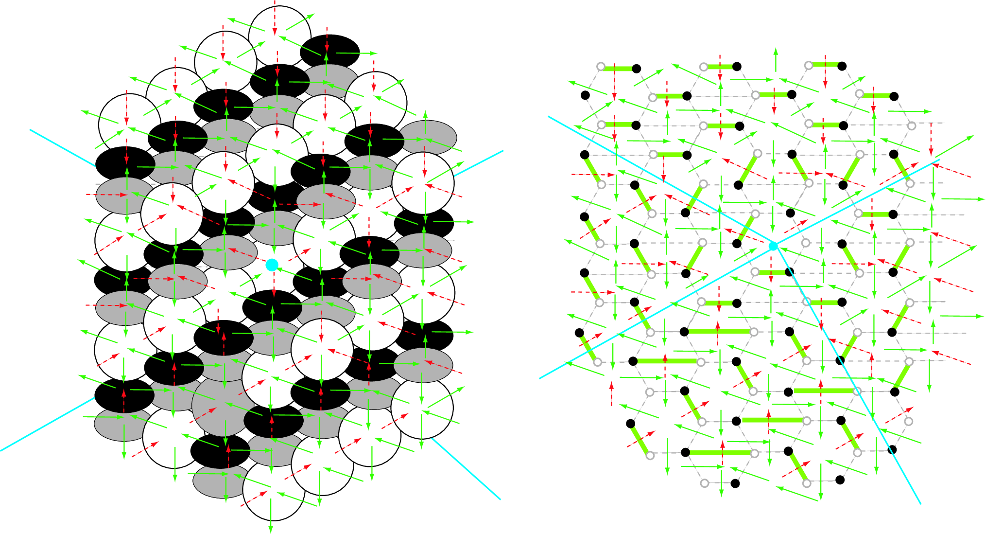
This defines a crystalline structure for an arbitrary toric Calabi-Yau manifold. In particular, it reproduces the crystal for discussed in [5, 2], and the one for conifold in [9]. See Figure 5 for the crystalline structure corresponding to the Suspended Pinched Point singularity. In this example, the ridge of the crystal (shown as blue lines in Figure 5) coincides with the -web of the toric geometry. As we will discuss later, this is a general property of our crystal.

4.2 BPS State and Molten Crystal
In the forthcoming discussions, the crystal defined above will be identified with a single D6 brane with no D0 and D2 charges. Bound states with non-zero D0 and D2 charges are obtained by removing atoms following the rule specified below.
In [9, 10], the Donaldson-Thomas invariants are computed by using the symmetry of the moduli space corresponding to translational invariance of . By the standard localization techniques, the Euler number can be evaluated at the fixed point set of the moduli space under the symmetry. Correspondingly, in the gauge theory side, BPS states counted by the index are those that are invariant under the global symmetry acting on bifundamental fields preserving the F-term constraints since those do not have extra zero modes and do not contribute to the index. We are interested in counting such BPS states.
In order for a molten crystal to correspond to invariant -stable -modules, we need to impose the following rule to remove atoms from the crystal. Let be a finite set of atoms to be removed from the crystal.
The Melting Rule: If is in for some , then should also be in .
Since atoms of the crystal correspond to elements of , we used the natural action of on to define in the above. This means that crystal melting starts at the peak at and takes place following paths in . An example of a molten crystal satisfying this condition is shown in Figure 6.

The melting rule means that a complement of the vector space spanned by in gives an ideal of . To see this, we just need to take the contraposition of the melting rule. It states: For any and for any , is also in .
Generally speaking, an ideal of an algebra defines a module. To see this, consider a vector which is annihilated by all elements of the ideal . From , we can generate a finite dimensional representation of the algebra by acting elements of on it. However, the converse is not always true. Fortunately, when modules are -stable and invariant under the symmetry, it was shown in [9, 10] that there is a one-to-one correspondence between ideals and modules. It follows that our molten crystal configurations are also in one-to-one correspondence with -modules and therefore with relevant BPS bound states of D branes. This proves that the statistical model of crystal melting computes the index of D brane bound states.
It would be instructive to understand explicitly how each molten crystal configuration corresponds to a BPS bound state. Starting from a molten crystal specified by , Prepare a one-dimensional vector space with basis vector for each atom . For each arrow of , define the action of on by when the arrow begins from and ends an another atom . Otherwise is defined to be zero. Since an arbitrary path is generated by concatenation of arrows, we have defined an action of on each . By linearly extending the action of onto the total space , we obtain a -module .
There are several special properties about this module . First, the F-term relations are automatically satisfied. This is because when there exists two different paths starting at and ending at , and are both defined to be . Second, by construction is generated by action of the algebra on a single element . In such a case is called a cyclic -module, and by lemma 2.3 of [10] is also -stable. Third, by the cyclicity of the module it follows that is invariant up to gauge transformations. Therefore, is a invariant -stable module. It follows from the result of [10] discussed at the beginning of this section that indeed corresponds a bound state of D branes contributing to the Witten index.
At the beginning of this subsection, we stated without explanation that the original crystal corresponds to a single D6 brane with no D0 and D2 charges, and removing atoms correspond to adding the D brane charges. To understand this statement, let us recall that, in section 2, we started with a configuration of D0 and D2 branes on the toric Calabi-Yau manifold and took a T-duality along the fiber to arrive at the brane configuration. Thus, the number of D2 branes at each node of the quiver diagram is a combination of D0 and D2 charges before T-duality. It is this number that is equal to the rank of the gauge group at .
By using the projection , the -module is decomposed as as we saw in section 3, where
| (4.1) |
In particular, the formula (4.1) means that the rank of the gauge group at the node is equal to the number of atoms with the color corresponding to the node that have been removed from the crystal. Thus, removing an atom at the node is equivalent to adding D0 and D2 charges carried by the node . It is interesting to note that each atom in the crystal does not correspond to a single D0 brane or a single D2 brane, but each of them carries a specific combination of D0 and D2 charges. In the crystal melting picture, fundamental constituents are not D0 and D2 branes but the atoms. This reminds us of the quark model of Gell-Mann and Zweig, where the fundamental constituents carry combinations of quantum numbers of hadrons, as opposed to the Sakata model, where existing elementary particles such as the proton, neutron and particle are chosen as fundamental constituents.
4.3 Observations on the Crystal Melting Model
We would like to make a few observations on the statistical model of crystal melting that counts the number of BPS bound states of D branes.
We have studied several examples of toric Calabi-Yau manifolds and found that the crystal structure in each case matches with the toric diagram. In particular, the ridges of the crystal, when projected onto the plane, line up with the web of the maximally degenerate toric diagram. This phenomenon is discussed in Appendix. There, we also explain the correspondence between molten crystal configurations and perfect matching of the bipartite graph introduced in section 2.2.
So far, we have considered molten crystals that are obtained by removing a few atoms. We may call them low temperature configurations. The high temperature behavior of the model, describing bound states with large D0 and D2 charges, is also interesting. For , it was shown in [5, 2] that the high temperature limit of the crystal melting model reproduces the geometric shape of the mirror manifold. Since the high temperature limit of a general statistical model of random perfecting matchings is known to be described by a certain plane algebraic curve [54], it would be interesting to understand its relation to the mirror of a general toric Calabi-Yau manifold [55].
In the last subsection, we found it useful to describe BPS bound states using ideals of the algebra . In the case when the toric Calabi-Yau manifold is , ideals are closely related to the quantization of the toric structure as discussed in [2]. The gauge theory for is the dimensional reduction of the supersymmetric Yang-Mills theory in four dimensions down to one dimension, and the bifundamental fields are three adjoint fields. The F-term and D-term conditions require that they all commute with each other. Thus chiral ring is generated by three elements which commute with each other without any further relation. In this case, any ideal is characterized by the three-dimensional Young diagram . Locate each box in the 3d Young diagram by the Cartesian coordinates () of the corner of the box most distant from the origin, and define to be a set of the 3d Cartesian coordinates for boxes in . We can then define the ideal of the chiral ring by,
| (4.2) |
In [2], this description was obtained by quantizing the toric geometry by using its canonical Kähler form and by identifying as states in the Hilbert space.
This can be generalized to an arbitrary toric Calabi-Yau manifold as follows. One starts with the quiver diagram corresponding to and use the brane tiling to identify the F-term equations. This gives the chiral ring generated by bifundamental fields obeying the F-term and D-term relations. As we saw in section 4.3, each BPS bound state is related to an ideal of the chiral algebra. We expect that such ideals arise from quantization of the toric structure. BPS bound states of D branes emerging from the quantization of background geometry is reminiscent of the bubbling AdS space of [56] and Mathur’s conjecture on black hole microstates [57].
5 Summary and Discussion
In this paper, we established the connection between the counting of BPS bound states of D0 and D2 branes on a single D6 brane to the non-commutative Donaldson-Thomas theory. We studied the moduli space of solutions to the F-term and D-term constraints of the quiver gauge theory which arises as the low energy limit of the brane configuration. We found the direct correspondence between the gauge theory moduli space and the space of modules of the factor algebra of the path algebra for the quiver diagram quotiented by its ideal related to the F-term constraints, subject to a stability condition to enforce the D-term constraints. Using this correspondence, we found a new description of BPS bound states of the D branes in terms of the statistical model of crystal melting. The crystalline structure is determined by the quiver diagram and the brane tiling which characterize the low energy effective theory of D branes. The crystal is composed of atoms of different colors, each of which corresponds to a node of the quiver diagram, and the chemical bond is dictated by the arrows of the quiver diagram. BPS states are constructed by removing atoms from the crystal.
The relation between the commutative and non-commutative Donaldson-Thomas invariant has been extensively discussed in the recent literature. The degeneracy of D brane bound states changes when the value of , used to define the stability condition, jumps along the codimension one subspace, which is called walls of marginal stability. The jump in the degeneracy can be computed by the wall crossing formula [58, 59, 60], and if we start from a particular chamber and applying wall crossing formula, we can obtain the value of in any chamber we want. In the example of conifold [13], wall crossing relates non-commutative Donaldson-Thomas invariants to commutative Donaldson-Thomas invariants and to new invariants defined by Pandharipande and Thomas [61]. This story is further generalized by [14] when has no internal lattice point. When the toric diagram contains an internal lattice point, non-commutative Donaldson-Thomas invariant includes D4 branes, since . Since (commutative) Donaldson-Thomas invariants does not include D4 brane charges, the above discussion of wall crossing should be modified.
It has been proven recently that the topological string theory is equivalent to the commutative Donaldson-Thomas theory for a general toric Calabi-Yau manifold [2, 8]. Since the commutative Donaldson-Thomas theory count BPS states for some choice of stability condition,
| (5.1) |
is indeed true in some chamber. On the other hand, our result shows that the relation,
| (5.2) |
holds in another chamber, where is the BPS state counting for another choice of the stability condition. Combining these two results, we find that the topological string theory and the statistical model of crystal melting are related by the wall crossing, and we have
| (5.3) |
Since there is no wall crossing phenomenon for the Donaldson-Thomas theory on , this result does not contradict with [2], where a direct identification of the topological string theory and the crystal melting is made for . In general, we expect that a proper understanding of the relation between the topological string theory and the crystal melting requires that we take the wall crossing phenomena into account.
The OSV formula (1.1) suggests yet another relation between the black hole microstate counting and the topological string theory. According to [62], for a compact Calabi-Yau manifold, the D6/D2/D0 brane system gives rise to a large black hole in four dimensions since it is related to a spinning M theory black hole by the Kaluza-Klein reduction. In fact, one can compute the semi-classical Bekenstein-Hawking entropy for such a 4-dimensional black hole and find that it can be made arbitrarily large provided the D2 charges are sufficiently larger than the D0 charge. In this paper, we discussed the D6/D2/D0 system on a non-compact toric Calabi-Yau manifold with an infinite volume. Though it is not obvious that the gravity description in four dimensions is applicable in this case, the OSV formula has been successfully tested for a similar class of non-compact Calabi-Yau manifolds [63, 64, 65, 66]. If it is applicable in our case, it would imply the relation between and , modulo wall crossings. It would be interesting to find out if such a relation holds.
It appears that the crystal melting picture is closely related to the quantization of the toric structure of the Calabi-Yau manifold. It would be interesting to understand the relation better. This could lead to a new insight into quantum geometry, along with the observations in [56] for the bubbling AdS geometry and [57] for black hole microstates.
Acknowledgments
We would like to thank Kentaro Nagao, Kazutoshi Ohta, Yukinobu Toda, Kazushi Ueda and Xi Yin for discussions. This work is supported in part by DOE grant DE-FG03-92-ER40701 and by the World Premier International Research Center Initiative of MEXT of Japan. H. O. is also supported in part by a Grant-in-Aid for Scientific Research (C) 20540256 of JSPS and by the Kavli Foundation. M. Y. is also supported in part by the JSPS fellowships for Young Scientists and by the Global COE Program for Physical Sciences Frontier at the University of Tokyo funded by MEXT of Japan.
Appendix A Perfect Matchings
In this Appendix we are going to explain the one-to-one correspondence between a molten crystal discussed in the main text and a perfect matching of the bipartite graph. This means that the problem of counting BPS states can also be reformulated as a problem of counting perfect matchings of the bipartite graph, where a perfect matching is a subset of edges of the bipartite graph such that each vertex is contained exactly once. The contents of this appendix is basically a recapitulation of [10].
In section 4.1 we considered a quiver , which is a universal cover of the quiver on . The dual graph of , which we denote by , can be made bipartite using orientation of arrows of , and is a universal cover of the bipartite graph on described in section 2.2. What we are going to do is to give an explicit correspondence between a perfect matching of the bipartite graph and a configuration of molten crystal.
We first construct a perfect matching from a molten crystal. Given a molten crystal as shown in Figure 5, choose all the arrows of which are along the surface of the crystal. In the example of Figure 5, such arrows are colored green in Figure 5, while the remaining arrows are colored red. Take the set of the dual of edges colored red. It is proven by [10] that such a subset of edges of is a perfect matching. This is the perfect matching we wanted to construct.
In the case when no atoms are removed from the crystal, the perfect matching obtained by this method is called the canonical perfect matching, which we denote by . Since only a finite number of atoms are removed from the crystal, the perfect matching obtained from a molten crystal by the above method coincides with when sufficiently away from the reference point .
Conversely, given a perfect matching which coincides with when sufficiently away from the reference point , we can reproduce a molten crystal. Let us superimpose with , and we have a finite number of loops, as shown in Figure 8 in the case of Suspended Pinched Point. Define a height function such that
(1) when sufficiently away from .
(2) increases by one whenever we cross the loop and go inside it.
The example of for the case of Suspended Pinched Point is shown in Figure 8.

By removing atoms from each , we can construct a molten crystal. It was proven in [10] that the set of atoms removed from the crystal so defined satisfies the melting rule of section 4.2. This establishes the one-to-one correspondence between a molten crystal and a perfect matching of the bipartite graph, meaning that BPS states can also be counted by perfect matchings of the bipartite graph .
Finally, let us finish this Appendix by pointing out an interesting connection of the canonical perfect matching with toric geometry. The example of canonical perfect matching for the Suspended Pinched Point is shown in Figure 9. In this example, the asymptotic form of the bipartite graph has four different patterns. Each of four patterns is periodic and therefore an be thought of as a perfect matching of the bipartite graph on . In the brane tiling literature, a perfect matching on the bipartite graph on is known to correspond to one of the lattice points of the toric diagram [25, 40].1313 13 For this correspondence, we consider superimposition of perfect matchings and define a -valued height function, which is similar to the height function defined previously. We recognize that the four perfect matchings are identified with the four corners of the toric diagram in Figure 1-(a) and that the borders between different patters are identified with the blue lines in Figure 1-(b), which makes the -web of the diagram.
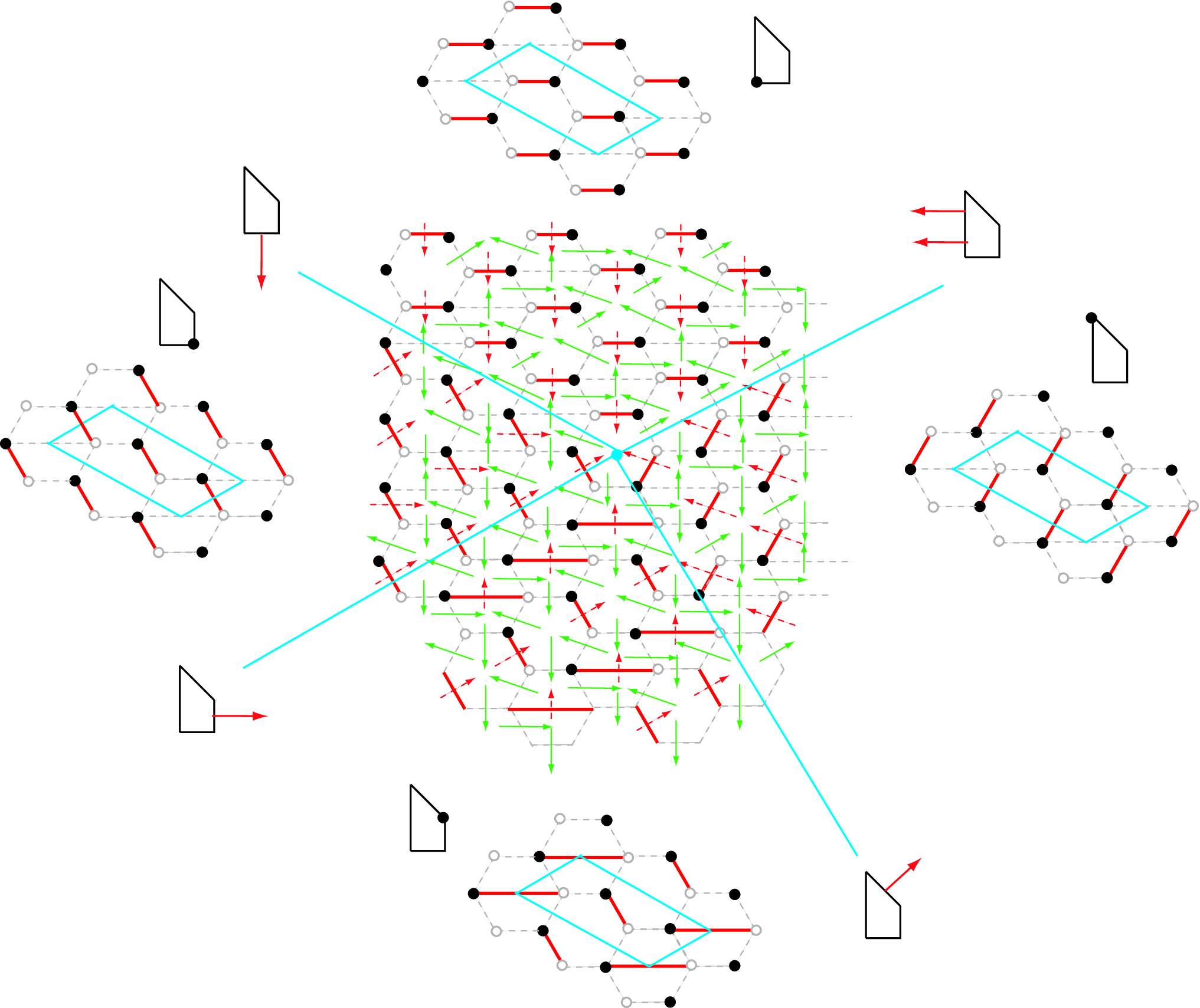
In general, for an arbitrary toric Calabi-Yau manifold, we can use the same pattern to construct a perfect matching. Divide the universal covering of the bipartite graph into segments separated by the -web of the toric diagram.1414 14 We choose the diagram that corresponds to the most singular Calabi-Yau manifold. The perfect matching in each segment is periodic and is identified with one of the perfect matchings of bipartite graphs on , which corresponds to one of the lattice points of the toric diagram and the lattice point in question is precisely the vertex surrounded by the two -webs on .1515 15 In a consistent quiver gauge theory, it is believed that the multiplicity of perfect matchings at the vertices of the toric diagram is one [28]. This determines a perfect matching. In particular, this means that the ridges of the crystal line up with the -web of the toric diagram.
We have examined several other examples as well, and this pattern holds in all cases. Thus, we conjecture that the perfect matching constructed in this way is canonical. We would like to stress again that this conjecture is not needed to construct the crystal melting model. Here we are simply pointing out that, in the examples we have studied, the crystalline structures fit beautifully with the corresponding toric geometries.
References
- [1] H. Ooguri, A. Strominger and C. Vafa, “Black hole attractors and the topological string,” Phys. Rev. D 70, 106007 (2004) [arXiv:hep-th/0405146].
- [2] A. Iqbal, N. Nekrasov, A. Okounkov and C. Vafa, “Quantum foam and topological strings,” JHEP 0804, 011 (2008) [arXiv:hep-th/0312022].
- [3] S. K. Donaldson and R. P. Thomas, “Gauge theory in higher dimensions,” in The geometric universe: science, geometry and the work of Roger Penrose, Oxford Univ. Press, 1998.
- [4] R. P. Thomas, “A holomorphic Casson invariant for Calabi-Yau 3-folds, and bundles on K3 fibrations,” J. Diff. Geom. 54, 367 (2000) [arXiv:math.AG/9806111].
- [5] A. Okounkov, N. Reshetikhin and C. Vafa, “Quantum Calabi-Yau and classical crystals,” arXiv:hep-th/0309208.
- [6] D. Maulik, N. Nekrasov, A. Okounkov and R. Pandharipande, “Gromov-Witten theory and Donaldson-Thomas theory. I,” Compos. Math. 142, 1263 (2006) [arXiv:math.AG/0312059].
- [7] M. Aganagic, A. Klemm, M. Marino and C. Vafa, “The topological vertex,” Commun. Math. Phys. 254, 425 (2005) [arXiv:hep-th/0305132].
- [8] D. Maulik, A. Oblomkov, A. Okounkov, R. Pandharipande, “Gromov-Witten/Donaldson-Thomas correspondence for toric 3-folds,” arXiv:0809.3976 [math.AG]
- [9] B. Szendröi, “Non-commutative Donaldson-Thomas theory and the conifold,” Geom. Topol. 12, 1171 (2008) [arXiv:0705.3419 [math.AG]].
- [10] S. Mozgovoy and M. Reineke, “On the noncommutative Donaldson-Thomas invariants arising from brane tilings,” arXiv:0809.0117 [math.AG].
- [11] B. Young, “Computing a pyramid partition generating function with dimer shuffling,” arXiv:0709.3079 [math.CO].
- [12] B. Young, with an appendix by J. Bryan, “Generating functions for colored 3D Young diagrams and the Donaldson-Thomas invariants of orbifolds,” arXiv:0802.3948 [math.CO].
- [13] K. Nagao and H. Nakajima, “Counting invariant of perverse coherent sheaves and its wall-crossing,” arXiv:0809.2992 [math.AG].
- [14] K. Nagao, “Derived categories of small toric Calabi-Yau 3-folds and counting invariants,” arXiv:0809.2994 [math.AG].
- [15] D. L. Jafferis and G. W. Moore, “Wall crossing in local Calabi Yau manifolds,” arXiv:0810.4909 [hep-th].
- [16] W. Y. Chuang and D. L. Jafferis, “Wall Crossing of BPS States on the Conifold from Seiberg Duality and Pyramid Partitions,” arXiv:0810.5072 [hep-th].
- [17] N. Saulina and C. Vafa, “D-branes as defects in the Calabi-Yau crystal,” arXiv:hep-th/0404246.
- [18] S. H. Katz, “Gromov-Witten, Gopakumar-Vafa, and Donaldson-Thomas invariants of Calabi-Yau threefolds,” arXiv:math/0408266.
- [19] T. Okuda, “Derivation of Calabi-Yau crystals from Chern-Simons gauge theory,” JHEP 0503, 047 (2005) [arXiv:hep-th/0409270].
- [20] R. Dijkgraaf, C. Vafa and E. Verlinde, “M-theory and a topological string duality,” arXiv:hep-th/0602087.
- [21] P. Sulkowski, “Crystal model for the closed topological vertex geometry,” JHEP 0612, 030 (2006) [arXiv:hep-th/0606055].
- [22] R. Dijkgraaf, D. Orlando and S. Reffert, “Dimer models, free fermions and super quantum mechanics,” arXiv:0705.1645 [hep-th].
- [23] D. L. Jafferis, “Topological Quiver Matrix Models and Quantum Foam,” arXiv:0705.2250 [hep-th].
- [24] J. J. Heckman and C. Vafa, “Crystal melting and black holes,” JHEP 0709, 011 (2007) [arXiv:hep-th/0610005].
- [25] A. Hanany and K. D. Kennaway, “Dimer models and toric diagrams,” arXiv:hep-th/0503149.
- [26] S. Franco, A. Hanany, K. D. Kennaway, D. Vegh and B. Wecht, “Brane dimers and quiver gauge theories,” JHEP 0601, 096 (2006) [arXiv:hep-th/0504110].
- [27] S. Franco, A. Hanany, D. Martelli, J. Sparks, D. Vegh and B. Wecht, “Gauge theories from toric geometry and brane tilings,” JHEP 0601, 128 (2006) [arXiv:hep-th/0505211].
- [28] A. Hanany and D. Vegh, “Quivers, tilings, branes and rhombi,” JHEP 0710, 029 (2007) [arXiv:hep-th/0511063].
- [29] K. D. Kennaway, “Brane Tilings,” Int. J. Mod. Phys. A 22, 2977 (2007) [arXiv:0706.1660 [hep-th]].
- [30] M. Yamazaki, “Brane Tilings and Their Applications,” Fortsch. Phys. 56, 555 (2008) [arXiv:0803.4474 [hep-th]].
- [31] M. R. Douglas and G. W. Moore, “D-branes, Quivers, and ALE Instantons,” arXiv:hep-th/9603167.
- [32] B. Feng, Y. H. He, K. D. Kennaway and C. Vafa, “Dimer models from mirror symmetry and quivering amoebae,” Adv. Theor. Math. Phys. 12, 3 (2008) [arXiv:hep-th/0511287].
- [33] H. Ooguri and C. Vafa, “Two-Dimensional Black Hole and Singularities of CY Manifolds,” Nucl. Phys. B 463 (1996) 55 [arXiv:hep-th/9511164].
- [34] Y. Imamura, “Anomaly Cancellations In Brane Tilings,” JHEP 0606, 011 (2006) [arXiv:hep-th/0605097].
- [35] Y. Imamura, “Global symmetries and ’t Hooft anomalies in brane tilings,” JHEP 0612, 041 (2006) [arXiv:hep-th/0609163].
- [36] Y. Imamura, H. Isono, K. Kimura and M. Yamazaki, “Exactly marginal deformations of quiver gauge theories as seen from brane tilings,” Prog. Theor. Phys. 117, 923 (2007) [arXiv:hep-th/0702049].
- [37] I. R. Klebanov and E. Witten, “Superconformal field theory on threebranes at a Calabi-Yau singularity,” Nucl. Phys. B 536, 199 (1998) [arXiv:hep-th/9807080].
- [38] I. R. Klebanov and M. J. Strassler, “Supergravity and a confining gauge theory: Duality cascades and SB-resolution of naked singularities,” JHEP 0008, 052 (2000) [arXiv:hep-th/0007191].
- [39] Y. Imamura, K. Kimura and M. Yamazaki, “Anomalies and O-plane charges in orientifolded brane tilings,” JHEP 0803, 058 (2008) [arXiv:0801.3528 [hep-th]].
- [40] S. Franco and D. Vegh, “Moduli spaces of gauge theories from dimer models: Proof of the correspondence,” JHEP 0611, 054 (2006) [arXiv:hep-th/0601063].
- [41] M. A. Luty and W. Taylor, “Varieties of vacua in classical supersymmetric gauge theories,” Phys. Rev. D 53, 3399 (1996) [arXiv:hep-th/9506098].
- [42] A. D. King, “Moduli of representations of finite dimensional algebras,” Quart. J. Math. Oxford 45, 515 (1994).
- [43] M. Cirafici, A. Sinkovics and R. J. Szabo, “Cohomological gauge theory, quiver matrix models and Donaldson-Thomas theory,” arXiv:0803.4188 [hep-th].
- [44] P. S. Aspinwall, “D-branes on Calabi-Yau manifolds,” arXiv:hep-th/0403166.
- [45] M. Van den Bergh, “Non-commutative crepant resolutions,” The legacy of Niels Henrik Abel, Springer, Berlin, 749 (2004) [arXiv:math.RA/0211064].
- [46] T. Bridgeland, “Flops and derived categories,” Invent. Math. 147, 613 (2002), [arXiv:math.AG/0009053]
- [47] M. Van den Bergh, “Three-dimensional flops and non-commutative rings,” Duke Math. J. 122, 423 (2004) [arXiv:math.AG/0207170].
- [48] K. Ueda and M. Yamazaki, “Brane tilings for parallelograms with application to homological mirror symmetry,” arXiv:math.AG/0606548.
- [49] K. Ueda and M. Yamazaki, “Homological mirror symmetry for toric orbifolds of toric del Pezzo surfaces,” arXiv:math.AG/0703267.
- [50] M. R. Douglas, B. Fiol and C. Romelsberger, “Stability and BPS branes,” JHEP 0509, 006 (2005) [arXiv:hep-th/0002037].
- [51] T. Bridgeland, “Stability conditions on triangulated categories,” Ann. of Math. 166, 317 (2007) [arXiv:math.AG/0212237].
- [52] S. K. Donaldson, “Anti self-dual Yang-Mills connections over complex algebraic surfaces and stable vector bundles,” Proc. London Math. Soc. 50, 1 (1985).
- [53] K. Uhlenbeck and S. -T. Yau, “On the existence of Hermitian-Yang-Mills connections in stable vector bundles,” Comm. Pure Appl. Math. 39, 257 (1986).
- [54] R. Kenyon, A. Okounkov and S. Sheffield, “Dimers and Amoebae,” arXiv:math-ph/0311005.
- [55] H. Ooguri and M. Yamazaki, work in progress.
- [56] H. Lin, O. Lunin and J. M. Maldacena, “Bubbling AdS space and 1/2 BPS geometries,” JHEP 0410, 025 (2004) [arXiv:hep-th/0409174].
- [57] S. D. Mathur, “The fuzzball proposal for black holes: An elementary review,” Fortsch. Phys. 53, 793 (2005) [arXiv:hep-th/0502050].
- [58] F. Denef and G. W. Moore, “Split states, entropy enigmas, holes and halos,” arXiv:hep-th/0702146.
- [59] M. Kontsevich and Y. Soibelman, “Stability structures, motivic Donaldson-Thomas invariants and cluster transformations,” to appear.
- [60] D. Gaiotto, G. W. Moore and A. Neitzke, “Four-dimensional wall-crossing via three-dimensional field theory,” arXiv:0807.4723 [hep-th].
- [61] R. Pandharipande and R. P. Thomas, “Curve counting via stable pairs in the derived category,” arXiv:0707.2348 [math.AG].
- [62] D. Gaiotto, A. Strominger and X. Yin, “New Connections Between 4D and 5D Black Holes,” JHEP 0602, 024 (2006) [arXiv:hep-th/0503217].
- [63] C. Vafa, “Two dimensional Yang-Mills, black holes and topological strings,” arXiv:hep-th/0406058.
- [64] M. Aganagic, H. Ooguri, N. Saulina and C. Vafa, “Black holes, q-deformed 2d Yang-Mills, and non-perturbative topological strings,” Nucl. Phys. B 715, 304 (2005) [arXiv:hep-th/0411280].
- [65] R. Dijkgraaf, R. Gopakumar, H. Ooguri and C. Vafa, “Baby universes in string theory,” Phys. Rev. D 73, 066002 (2006) [arXiv:hep-th/0504221].
- [66] M. Aganagic, H. Ooguri and T. Okuda, “Quantum entanglement of baby universes,” Nucl. Phys. B 778, 36 (2007) [arXiv:hep-th/0612067].