跳到论文正文
W Papers独立论文阅读器 arXiv:0811.2777 论文正文 计算阅读时间 · 0%
引用这篇论文根据当前论文元数据生成,正式投稿前建议核对。


License: arXiv.org perpetual non-exclusive license
arXiv:0811.2777v2 [math.DS] 03 Feb 2010

The Julia set of a post-critically finite endomorphism of ℙ​ℂ2\mathbb{P}\mathbb{C}^{2}Thanks: This paper is based upon work supported by the National Science Foundation under Grants DMS0605019 and DMS0800085.

Volodymyr Nekrashevych
Abstract.

We construct a combinatorial model of the Julia set of the endomorphism f⁡(z,w)=((1−2​z/w)2,(1−2/w)2)f(z,w)=((1-2z/w)^{2},(1-2/w)^{2}) of ℙ​ℂ2\mathbb{P}\mathbb{C}^{2}.

1. Introduction

J. E. Fornæss and N. Sibony studied in [FS92] two post-critically finite endomorphisms of ℙ​ℂ2\mathbb{P}\mathbb{C}^{2}. The Julia set of one of them is ℙ​ℂ2\mathbb{P}\mathbb{C}^{2}, while the Julia set of the other has no interior.

The latter map appeared independently in [BN06] as a natural skew product map in the study of Thurston equivalence of topological polynomials with the post-critical dynamics of z2+iz^{2}+i. It is written in affine coordinates as

f(z,w)=((1−2​zw)2,(1−2w)2).f\left(z,w\right)=\left(\left(1-\frac{2z}{w}\right)^{2},\quad\left(1-\frac{2}{w}\right)^{2}\right).

As a development of [BN06], group theoretic aspects of the map ff were studied in [Nek07] and [Nek10]. The iterated monodromy group of ff was used to construct an uncountable family of three-generated groups with interesting properties, and later a new group of non-uniform exponential growth was found in this family (the first examples of groups of non-uniform exponential growth were found in [Wil04]).

In the current paper we apply our group theoretic knowledge to description of the Julia set of ff. We construct a combinatorial model of the Julia set in the spirit of Hubbard trees. Of course, here the Hubbard trees become “Hubbard complexes” (actually even complexes of groups); but due to a particular skew product structure of the map, the Hubbard complex of ff is a bundle of “Hubbard tripods”, and the combinatorial model of the Julia set can be described in terms of a “folding map” on the bundle of tripods. The Julia set of ff is represented then as the projective limit of a sequences of three-dimensional Hubbard complexes, which are homeomorphic to subsets of the Julia set.

A general method of constructing similar combinatorial models of expanding dynamical systems is described in [Nek08a]. Finding simple and elegant models is still of interest, since construction from [Nek08a] depends on some choices, which can be made in different ways, leading to models of different complexity.

Interesting examples of post-critically finite multi-dimensional maps come from the study of correspondences on the moduli space of a punctured sphere, see [BN06, Koc07, Nek08a].

Unfortunately, an important ingredient of our analysis is missing. I was not able to prove that ff is sub-hyperbolic, i.e., to construct a singular metric on a neighborhood of the Julia set of ff, such that ff is uniformly expanding with respect to it.

1.1. Overview of the paper

The second section of the paper collects elementary and previously known properties of the function ff. We describe its action on the projective plane ℙ​ℂ2\mathbb{P}\mathbb{C}^{2}, the structure of the post-critical set of ff, recall the results of J. E. Fornæss and N. Sibony and discuss the skew product structure of the map.

Section “Techniques” is an overview of the theory of self-similar groups, iterated monodromy groups and their limit spaces. There are no proofs in it, which can be found either in [Nek05], or in [Nek08a]. In particular, the general notion of combinatorial models of expanding dynamical systems is described in this section. More on combinatorial models of hyperbolic dynamical systems, see [IS08] and [Nek08a].

We compute the iterated monodromy group of ff in Section 4. We use an interpretation of the map ff given in [BN06], which makes it possible to compute the iterated monodromy group IMG(f)\mathop{\mathrm{IMG}}(f) in a relatively easy way.

The combinatorial model of ff is constructed in Section 5. It is convenient to pass to an index 2 extension Γ\Gamma of IMG(f)\mathop{\mathrm{IMG}}(f). This extension can be defined as the iterated monodromy group of the quotient of the dynamical system (f,ℙ​ℂ2)(f,\mathbb{P}\mathbb{C}^{2}) by the group of order two generated by the transformation (z,w)↦(z¯,w¯)(z,w)\mapsto(\overline{z},\overline{w}). The group Γ\Gamma is generated by a relatively small automaton (of 12 states). It has appeared for the first time in [Nek07], where it was used to study a Cantor set of groups associated with ff. We continue the study of the group Γ\Gamma in Section 5 of our paper. In particular, we describe its nucleus, which happens to be a union of six finite groups. We use the poset of subgroups of the nucleus to construct a simplicial complex, serving as the first approximation of the limit space of Γ\Gamma.

This complex consists of three tetrahedra with one common face. The corresponding approximation of the Julia set of ff is obtained by pasting together two copies of this complex. We construct the combinatorial model of the Julia set (in Subsection 5.6); give an inductive cut-and-paste rule for constructing a sequences of polyhedra approximating the Julia set (Theorem 5.4 and Proposition 5.8); and prove that Julia set is the inverse limit of the constructed polyhedra (Theorem 5.7).

The cut-and-paste rule works as follows. The nnth level approximation ℳn\mathcal{M}_{n} of the Julia set is obtained by pasting together two copies of a complex 𝒯n\mathcal{T}_{n} along their “boundary”. The boundary of 𝒯n\mathcal{T}_{n} is decomposed into a union of 11 regions, which are domains of involutive maps κg,n\kappa_{g,n} (“pasting rules”). The next complex 𝒯n+1\mathcal{T}_{n+1} is obtained by pasting four copies of 𝒯n\mathcal{T}_{n} using five of the maps κg,n\kappa_{g,n}. The 11 pieces of the boundary of 𝒯n+1\mathcal{T}_{n+1} and the corresponding maps κg,n+1\kappa_{g,n+1} are defined then as unions of the pieces of the boundaries of the copies of 𝒯n\mathcal{T}_{n} according to rules described by the finite automaton generating the group Γ\Gamma.

The rules are not very complicated, but since the complexes are three dimensional and can not be embedded into ℝ3\mathbb{R}^{3} without self-intersections, it is hard to visualize them.

In order to understand better the constructed polyhedral model of the Julia set, we use the skew product structure of ff (and of the model), and study it “fiberwise” in Section 6. We show that the fibers of the complexes ℳn\mathcal{M}_{n} are trees that can be constructed using natural “folding” and “unfolding” transformation (Theorem 6.2 and Proposition 6.6). As a limit of iterations of the folding and unfolding procedures we get dendrites homeomorphic to the intersections of the Julia set of ff with the lines w=w0w=w_{0}.

Our models are very similar to the usual Hubbard trees, since the approximating complexes ℳn\mathcal{M}_{n} are homeomorphic to the subsets f−n​(ℳ)f^{-n}(\mathcal{M}), where ℳ\mathcal{M} is a “span” of the post-critical set of ff inside the Julia set of ff (Proposition 6.8).

The last section of our paper contains additional results deduced from the model of the Julia set and from properties of the iterated monodromy group of ff. We construct a family of length metrics on the slices of the Julia set of ff; define a family of natural surjections of the slices onto an isosceles right triangle (this includes, for instance, the Sierpiński plane-filling curve as a particular case); describe when the slices are finite trees; and describe the action of ff on the manifold of “external rays” of the Julia set of ff. It is shown that the manifold of external rays is an orbispace with the universal covering identified with the real Heisenberg group, so that the action of ff is induced by an expanding automorphism of the Heisenberg group. Note that in the classical case of polynomials of degree dd the space of external rays is ℝ/ℤ\mathbb{R}/\mathbb{Z} with the action of the polynomial induced by the automorphism x↦d⋅xx\mapsto d\cdot x of ℝ\mathbb{R}.

2. The rational function

Consider the transformation of ℂ2\mathbb{C}^{2}

f(z,w)=((1−2​zw)2,(1−2w)2).f\left(z,w\right)=\left(\left(1-\frac{2z}{w}\right)^{2},\quad\left(1-\frac{2}{w}\right)^{2}\right).

It can be extended to a map f:ℙ​ℂ2→ℙ​ℂ2f:\mathbb{PC}^{2}\rightarrow\mathbb{PC}^{2} as

f:[z:w:u]↦[(w−2z)2:(w−2u)2:w2].f:[z:w:u]\mapsto[(w-2z)^{2}:(w-2u)^{2}:w^{2}].

The Jacobian of the map ff is then

|−4​(w−2​z)002​(w−2​z)2​(w−2​u)2​w0−4​(w−2​u)0|=−32​(w−2​z)​(w−2​u)​w,\left|\begin{array}[]{ccc}-4(w-2z)&0&0\\ 2(w-2z)&2(w-2u)&2w\\ 0&-4(w-2u)&0\end{array}\right|=-32(w-2z)(w-2u)w,

Hence, the critical locus is the union of the lines w=2​zw=2z, w=2​uw=2u, and w=0w=0. Their orbits are

{w=2z}↦{z=0}↦{z=u}↦{z=w}↦{z=u}\{w=2z\}\mapsto\{z=0\}\mapsto\{z=u\}\mapsto\{z=w\}\mapsto\{z=u\}

and

{w=2u}↦{w=0}↦{u=0}↦{w=u}↦{w=u}.\{w=2u\}\mapsto\{w=0\}\mapsto\{u=0\}\mapsto\{w=u\}\mapsto\{w=u\}.

Consequently, the post-critical set is the union of six lines

z=0,z=u,z=w,w=0,w=u,u=0,z=0,\quad z=u,\quad z=w,\quad w=0,\quad w=u,\quad u=0,

or, in affine coordinates: z=0z=0, z=1z=1, z=wz=w, w=0w=0, w=1w=1, and the line at infinity.

The function ff appeared in [BN06], where it was used to answer a question of J. Hubbard and A. Duady from [DH93] on combinatorial equivalence of some branched coverings of the plane. Groups associated with it were studied in [Nek07] and [Nek10].

This function is conjugate to the function

f~([z:w:t])=[(z−2w)2:z2:(z−2t)2],\widetilde{f}([z:w:t])=[(z-2w)^{2}:z^{2}:(z-2t)^{2}],

considered by J. E. Fornæss and N. Sibony in [FS92]. The conjugating map is

z↦w,w↦u,t↦z,z\mapsto w,\quad w\mapsto u,\quad t\mapsto z,

where the variables on the left-hand side are from [FS92], while the variables from the right-hand side are the ones used in our paper.

The following properties of the map ff are proved in [FS92]. Denote by VV the post-critical set of ff and by WW its full preimage f−1​(V)f^{-1}(V).

Theorem 2.1.

The sets ℙ​ℂ2∖V\mathbb{P}\mathbb{C}^{2}\setminus V and ℙ​ℂ2∖W\mathbb{P}\mathbb{C}^{2}\setminus W are Kobayashi hyperbolic and the map f:ℙ​ℂ2∖W→ℙ​ℂ2∖Vf:\mathbb{P}\mathbb{C}^{2}\setminus W\rightarrow\mathbb{P}\mathbb{C}^{2}\setminus V is noncontracting in the infinitesimal Kobayashi metric on ℙ​ℂ2∖V\mathbb{P}\mathbb{C}^{2}\setminus V.

The point [1:0:0][1:0:0] is a superattracting fixed point. Let UU be its basin of attraction and let J=ℙ​ℂ2∖UJ=\mathbb{P}\mathbb{C}^{2}\setminus U be its complement. Then UU is a topological cell and a Kobayashi hyperbolic domain of holomorphy.

The set JJ has no interior and is the Julia set of ff. The map ff is topologically transitive on JJ and repelling periodic points are dense in JJ.

The aim of our paper is to describe the combinatorics and topology of the Julia set JJ in the spirit of Hubbard trees (see [DH84, DH85, Poi93]).

Theorem 2.1 is not quite what we need to be able to apply the techniques of the iterated monodromy groups to the study of the Julia set of ff. The results of our paper are therefore true only modulo the following conjecture.

Conjecture.

There exists an orbispace metric on ℙℂ2∖{[1:0:0]}\mathbb{P}\mathbb{C}^{2}\setminus\{[1:0:0]\} such that ff is uniformly expanding with respect to this metric on a neighborhood of the Julia set.

In fact, some weaker results would be sufficient, but they are probably equivalent to the above conjecture. It would be very nice to have a general statement about sub-hyperbolicity of post-critically finite endomorphisms of complex projective spaces.

Note that the map ff has a skew product structure: the second coordinate is a rational function depending only on the second coordinate. On the first coordinates of iterations of ff we get compositions of quadratic polynomials fw​(z)=(1−2w​z)2f_{w}(z)=\left(1-\frac{2}{w}z\right)^{2}, i.e., non-autonomous iteration of quadratic polynomials. The critical point z=w/2z=w/2 of the polynomial fwf_{w} is mapped to 00, fw​(0)=1f_{w}(0)=1, and fw​(1)f_{w}(1) is equal to the next value (1−2w)2\left(1-\frac{2}{w}\right)^{2} of the second coordinate in the iteration of ff. We see that the non-autonomous iteration on the first coordinate is post-critically finite: the set of critical values of the composition fwn∘fwn−1∘⋯∘fw1f_{w_{n}}\circ f_{w_{n-1}}\circ\cdots\circ f_{w_{1}} belongs to the set {0,1,wn+1}\{0,1,w_{n+1}\}, where wi+1=(1−2wi)2w_{i+1}=\left(1-\frac{2}{w_{i}}\right)^{2} for i=1,…,ni=1,\ldots,n. For more on post-critically finite non-autonomous iterations of polynomials, see [Nek09].

It follows from the skew-product structure of the map ff that it agrees with the projection P:[z:w:u]↦[w:u]P:[z:w:u]\mapsto[w:u] (defined on the complement of the point [1:0:0][1:0:0]), which is written in affine coordinates as P:(z,w)↦wP:(z,w)\mapsto w. Namely, the fibers of the projection are mapped by ff to fibers. In particular, by Theorem 2.1, the fiber P−1​(w)∩JP^{-1}(w)\cap J of the projection P:J→ℂ^P:J\rightarrow\widehat{\mathbb{C}} of the Julia set of ff onto the sphere (which is the Julia set of (1−2w)2\left(1-\frac{2}{w}\right)^{2}) is the Julia set of the non-autonomous iteration

ℂ→fw0ℂ→fw1ℂ→fw2⋯,\mathbb{C}\xrightarrow{f_{w_{0}}}\mathbb{C}\xrightarrow{f_{w_{1}}}\mathbb{C}\xrightarrow{f_{w_{2}}}\cdots,

where w0=ww_{0}=w and wi+1=(1−2w)2w_{i+1}=\left(1-\frac{2}{w}\right)^{2}.

This makes it possible to draw the slices P−1​(w)∩JP^{-1}(w)\cap J of the Julia set of ff in zz-planes. See some of such slices on Figure 1.

Refer to caption
Figure 1. Intersections of the Julia set of ff with the zz-planes

The rational function appearing on the second coordinate of ff is a Lattès example. Namely, it is semiconjugate to the map z↦(i−1)​zz\mapsto(i-1)z on ℂ\mathbb{C}, where the semiconjugacy is the map

ℂ→ℙ​ℂ1:z↦(℘⁡(z))2,\mathbb{C}\rightarrow\mathbb{PC}^{1}:z\mapsto(\wp(z))^{2},

where ℘\wp is the Weierstrass’ function associated with the lattice of Gaussian integers ℤ⁡[i]\mathbb{Z}[i]. See a proof of this fact in [Mil04] and [BN06]. In other words, the rational function (1−2w)2\left(1-\frac{2}{w}\right)^{2} is conjugate to the map induced by z↦(i−1)​zz\mapsto(i-1)z on the orbifold of the action of the group of orientation-preserving isometries of the lattice ℤ⁡[i]\mathbb{Z}[i] of Gaussian integers.

3. Techniques

3.1. Self-similar groups

Definition 3.1.

A wreath recursion is a homomorphism ψ:G→𝔖⁡(𝖷)≀G\psi:G\rightarrow\mathfrak{S}\left(\mathsf{X}\right)\wr G from a group GG to the wreath product of GG with the symmetric group 𝔖⁡(𝖷)\mathfrak{S}\left(\mathsf{X}\right).

Here symmetric group 𝔖⁡(𝖷)\mathfrak{S}\left(\mathsf{X}\right) acts on 𝖷\mathsf{X} from the left. We will denote the identity element of a group by ε\varepsilon.

The wreath product 𝔖⁡(𝖷)≀G=𝔖⁡(𝖷)⋉G𝖷\mathfrak{S}\left(\mathsf{X}\right)\wr G=\mathfrak{S}\left(\mathsf{X}\right)\ltimes G^{\mathsf{X}} is the set of pairs (σ,(gx)x∈𝖷)(\sigma,(g_{x})_{x\in\mathsf{X}}), where σ∈𝔖⁡(𝖷)\sigma\in\mathfrak{S}\left(\mathsf{X}\right) and (gx)x∈𝖷(g_{x})_{x\in\mathsf{X}} is an element of the direct product G𝖷G^{\mathsf{X}}. The elements of the wreath product are multiplied by the rule

(σ,(gx)x∈𝖷)⋅(π,(hx)x∈𝖷)=(σ​π,(gπ⁡(x)​hx)x∈𝖷).(\sigma,(g_{x})_{x\in\mathsf{X}})\cdot(\pi,(h_{x})_{x\in\mathsf{X}})=(\sigma\pi,(g_{\pi(x)}h_{x})_{x\in\mathsf{X}}).

We will write the pair (σ,(gx)x∈𝖷)(\sigma,(g_{x})_{x\in\mathsf{X}}) as a product σ​(gx)x∈𝖷\sigma(g_{x})_{x\in\mathsf{X}}, identifying σ\sigma with (σ,(ε)x∈𝖷)(\sigma,(\varepsilon)_{x\in\mathsf{X}}) and (gx)x∈𝖷(g_{x})_{x\in\mathsf{X}} with (ε,(gx)x∈𝖷)(\varepsilon,(g_{x})_{x\in\mathsf{X}}). It is easy to see that this identification agrees with the multiplication rule. If 𝖷={1,2,…,d}\mathsf{X}=\{\mathit{1},\mathit{2},\ldots,d\}, then we write σ​(gx)x∈𝖷\sigma(g_{x})_{x\in\mathsf{X}} as a sequence σ⁡(g1,g2,…,gd)\sigma(g_{\mathit{1}},g_{\mathit{2}},\ldots,g_{d}).

Let ψ:G→𝔖⁡(𝖷)≀G\psi:G\rightarrow\mathfrak{S}\left(\mathsf{X}\right)\wr G be a wreath recursion. Then the associated permutation GG-bimodule 𝔐\mathfrak{M} is the set 𝖷×G\mathsf{X}\times G together with two (left and right) actions of GG on it that are given by the rules

(x,h)⋅g=(x,h​g),g⋅(x,h)=(σ⁡(x),gx​h),(x,h)\cdot g=(x,hg),\quad g\cdot(x,h)=(\sigma(x),g_{x}h),

for ψ⁡(g)=σ​(gx)x∈𝖷\psi(g)=\sigma(g_{x})_{x\in\mathsf{X}}. We will identify x∈𝖷x\in\mathsf{X} with (x,ε)∈𝔐(x,\varepsilon)\in\mathfrak{M} and write (x,g)=x⋅g(x,g)=x\cdot g.

If we compose a wreath recursion ψ:G→𝔖⁡(𝖷)≀G\psi:G\rightarrow\mathfrak{S}\left(\mathsf{X}\right)\wr G with an inner automorphism of 𝔖⁡(𝖷)≀G\mathfrak{S}\left(\mathsf{X}\right)\wr G, then we do not change the isomorphism class of the associated bimodule (see [Nek05, Proposition 2.3.4] or [Nek08b, Proposition 2.22]).

Definition 3.2.

A self-similar group (G,𝖷)(G,\mathsf{X}) is a group GG together with a wreath recursion ψ:G→𝔖⁡(𝖷)≀G\psi:G\rightarrow\mathfrak{S}\left(\mathsf{X}\right)\wr G. Self-similar groups defined by wreath recursions that differ by an inner automorphism of 𝔖⁡(𝖷)≀G\mathfrak{S}\left(\mathsf{X}\right)\wr G are called equivalent.

Equivalently, a self-similar group is a group GG together with a covering bimodule 𝔐\mathfrak{M}, as it is defined below.

Definition 3.3.

Let GG be a group. A permutational GG-bimodule is a set 𝔐\mathfrak{M} with commuting left and right actions of GG on it, i.e., maps G×𝔐→𝔐:(g,x)↦g⋅xG\times\mathfrak{M}\rightarrow\mathfrak{M}:(g,x)\mapsto g\cdot x and 𝔐×G→𝔐:(x,g)↦x⋅g\mathfrak{M}\times G\rightarrow\mathfrak{M}:(x,g)\mapsto x\cdot g such that ε⋅x=x⋅ε=x\varepsilon\cdot x=x\cdot\varepsilon=x for all x∈𝔐x\in\mathfrak{M} and

g1⋅(g2⋅x)=g1​g2⋅x,(x⋅g1)⋅g2=x⋅g1​g2,\displaystyle g_{1}\cdot(g_{2}\cdot x)=g_{1}g_{2}\cdot x,\qquad(x\cdot g_{1})\cdot g_{2}=x\cdot g_{1}g_{2},
(g1⋅x)⋅g1=g1⋅(x⋅g2),\displaystyle(g_{1}\cdot x)\cdot g_{1}=g_{1}\cdot(x\cdot g_{2}),

for all g1,g2∈Gg_{1},g_{2}\in G and x∈𝔐x\in\mathfrak{M}.

A permutational GG-bimodule is called a covering dd-fold bimodule if the right action of GG on 𝔐\mathfrak{M} has dd orbits and is free, i.e., if x⋅g=xx\cdot g=x implies g=εg=\varepsilon.

It is easy to see that the bimodule associated with a wreath recursion ψ:G→𝔖⁡(𝖷)≀G\psi:G\rightarrow\mathfrak{S}\left(\mathsf{X}\right)\wr G is a covering dd-fold bimodule for d=|𝖷|d=|\mathsf{X}|. In the other direction, if 𝔐\mathfrak{M} is a covering GG-bimodule, then for a given right orbit transversal 𝖷\mathsf{X} (i.e., such a subset 𝖷⊂𝔐\mathsf{X}\subset\mathfrak{M} that every right orbit contains exactly one element of 𝖷\mathsf{X}), we get the associated wreath recursion

g↦σ​(g|x)x∈𝖷,g\mapsto\sigma(g|_{x})_{x\in\mathsf{X}},

where σ∈𝔖⁡(𝖷)\sigma\in\mathfrak{S}\left(\mathsf{X}\right) and g|xg|_{x} are given by the condition

g⋅x=σ⁡(x)⋅g|xg\cdot x=\sigma(x)\cdot g|_{x}

in 𝔐\mathfrak{M}. The permutation σ\sigma is the associated action of gg on 𝖷\mathsf{X}. We get in this way an action of GG on 𝖷\mathsf{X} defined by the wreath recursion. More formally, this action is obtained by composing the wreath recursion with the projection of 𝔖⁡(𝖷)≀G\mathfrak{S}\left(\mathsf{X}\right)\wr G onto 𝔖⁡(𝖷)\mathfrak{S}\left(\mathsf{X}\right). We will usually denote g⁡(x)=σ⁡(x)g(x)=\sigma(x).

We say that a subset 𝖷⊂𝔐\mathsf{X}\subset\mathfrak{M} is a basis of the bimodule 𝔐\mathfrak{M}, if it a right orbit transversal. We will usually label the letters of 𝖷\mathsf{X} by integers 1,2,…,d\mathit{1},\mathit{2},\ldots,d, thus identifying 𝔖⁡(𝖷)\mathfrak{S}\left(\mathsf{X}\right) with 𝔖⁡(d)\mathfrak{S}\left(d\right). It is not hard to prove that changing the basis 𝖷\mathsf{X} amounts to composing the associated wreath recursion by an inner automorphism of 𝔖⁡(d)≀G\mathfrak{S}\left(d\right)\wr G (see [Nek05, Subsection 2.3.4] and [Nek08b, Proposition 2.22]).

The following result is proved in [Nek05, Section 2.5].

Proposition 3.1.

Let GG be a self-similar group with the associated wreath recursion ψ:G→𝔖⁡(𝖷)≀G\psi:G\rightarrow\mathfrak{S}\left(\mathsf{X}\right)\wr G. Suppose that the associated action on 𝖷\mathsf{X} is transitive. Then the wreath recursion, up to composition with an inner automorphism of 𝔖⁡(𝖷)≀G\mathfrak{S}\left(\mathsf{X}\right)\wr G, is uniquely determined for any x∈𝖷x\in\mathsf{X} by the homomorphism

g↦gx,g\mapsto g_{x},

from the stabilizer of xx into GG. Here gxg_{x} is the coordinate of ψ⁡(g)=σ​(gx)x∈𝖷\psi(g)=\sigma(g_{x})_{x\in\mathsf{X}} corresponding to xx.

The homomorphism g↦gxg\mapsto g_{x} defined on the stabilizer of xx is called the virtual endomorphism associated with the wreath recursion (or with self-similarity of the group).

The following proposition gives formulae for the wreath recursion with a given associated virtual endomorphism.

Proposition 3.2.

Let ϕ:G1→G\phi:G_{1}\rightarrow G be a virtual endomorphism of a group GG, where G1G_{1} is a subgroup of finite index in GG. Let {r1,r2,…,rd}\{r_{1},r_{2},\ldots,r_{d}\} be a left coset transversal of GG modulo G1G_{1} (i.e., a set such that GG is a disjoint union of the cosets ri⋅G1r_{i}\cdot G_{1}). Let {xi}i=1,…,d=𝖷\{x_{i}\}_{i=1,\ldots,d}=\mathsf{X} be an alphabet of size dd. For g∈Gg\in G put ψ⁡(g)=σ​(gx)x∈𝖷\psi(g)=\sigma(g_{x})_{x\in\mathsf{X}}, where σ⁡(xi)=xj\sigma(x_{i})=x_{j} if g​ri∈rj​G1gr_{i}\in r_{j}G_{1}, and gxi=ϕ⁡(rj−1​g​ri)g_{x_{i}}=\phi(r_{j}^{-1}gr_{i}). Then ψ:G→𝔖⁡(𝖷)≀G\psi:G\rightarrow\mathfrak{S}\left(\mathsf{X}\right)\wr G is a wreath recursion such that ϕ\phi is associated with it.

3.2. Iteration of the wreath recursion

Let (G,𝖷)(G,\mathsf{X}) be a self-similar group and let 𝔐=𝖷×G\mathfrak{M}=\mathsf{X}\times G be the associated permutational bimodule. For x∈𝖷x\in\mathsf{X} and g∈Gg\in G we denote

g⋅x=g⁡(x)⋅g|x.g\cdot x=g(x)\cdot g|_{x}.

If ψ\psi is the associated wreath recursion, then for ψ⁡(g)=σ​(gx)x∈𝖷\psi(g)=\sigma(g_{x})_{x\in\mathsf{X}} we have g⁡(x)=σ⁡(x)g(x)=\sigma(x) and g|x=gxg|_{x}=g_{x}.

We define then inductively, for a finite word v=x1​x2​…​xn∈𝖷∗v=x_{1}x_{2}\ldots x_{n}\in\mathsf{X}^{*} and g∈Gg\in G, a word g⁡(v)g(v) and an element g|v∈Gg|_{v}\in G by the rule

g⁡(x​v)=g⁡(x)​g|x​(v),g|x​v=g|x|v.g(xv)=g(x)g|_{x}(v),\qquad g|_{xv}=g|_{x}|_{v}.

It is easy to see that for every n≥1n\geq 1 the map σn,g:v↦g⁡(v)\sigma_{n,g}:v\mapsto g(v) is a permutation of the set 𝖷n\mathsf{X}^{n} and that the map

ψ⊗n:G→𝔖⁡(𝖷n)≀G:g↦σn,g​(g|v)v∈𝖷n\psi^{\otimes n}:G\rightarrow\mathfrak{S}\left(\mathsf{X}^{n}\right)\wr G:g\mapsto\sigma_{n,g}(g|_{v})_{v\in\mathsf{X}^{n}}

is a homomorphism. The wreath recursion ψ⊗n\psi^{\otimes n} is called the nnth iteration of the wreath recursion ψ\psi.

Let 𝖷∗=⨆n≥0𝖷n\mathsf{X}^{*}=\bigsqcup_{n\geq 0}\mathsf{X}^{n} be the rooted tree of finite words over 𝖷\mathsf{X}, where every word v∈𝖷∗v\in\mathsf{X}^{*} is connected to the words of the form v​xvx for x∈𝖷x\in\mathsf{X}. The empty word is the root of the tree 𝖷∗\mathsf{X}^{*}. It is easy to check that for every g∈Gg\in G the permutation v↦g⁡(v)v\mapsto g(v) of 𝖷∗\mathsf{X}^{*} is an automorphism of the rooted tree 𝖷∗\mathsf{X}^{*}, and that in this way we get an action of the group GG on the tree 𝖷∗\mathsf{X}^{*}. It is called the action associated with the bimodule (with the wreath recursion). This action, up to conjugacy of actions, depends only on the associated permutational bimodule (does not depend on the choice of the basis 𝖷\mathsf{X}).

Definition 3.4.

Let ψ:G→𝔖⁡(𝖷)≀G\psi:G\rightarrow\mathfrak{S}\left(\mathsf{X}\right)\wr G be a wreath recursion. A faithful quotient of GG (with respect to ψ\psi) is the quotient of GG by the kernel of the action on 𝖷∗\mathsf{X}^{*} associated with the wreath recursion ψ\psi.

The wreath recursion is interpreted then as a recurrent description of the action of the group elements on the tree 𝖷∗\mathsf{X}^{*}. For g∈Gg\in G such that ψ⁡(g)=σ​(g|x)x∈𝖷\psi(g)=\sigma(g|_{x})_{x\in\mathsf{X}}, the permutation σ∈𝔖⁡(𝖷)\sigma\in\mathfrak{S}\left(\mathsf{X}\right) describes the action of gg on the first level 𝖷\mathsf{X} of the tree 𝖷∗\mathsf{X}^{*}, while the coordinates g|xg|_{x} describe the action on the subtree x​𝖷∗x\mathsf{X}^{*}, so that

g⁡(x​v)=σ⁡(x)​g|x​(v)g(xv)=\sigma(x)g|_{x}(v)

for all v∈𝖷∗v\in\mathsf{X}^{*}. In general, we have

g⁡(v​w)=g⁡(v)​g|v​(w)g(vw)=g(v)g|_{v}(w)

for all v,w∈𝖷∗v,w\in\mathsf{X}^{*} and g∈Gg\in G. Note that if the action of GG on 𝖷∗\mathsf{X}^{*} is faithful, then the above equality uniquely determines g|vg|_{v}. The elements g|vg|_{v} are called the sections of the element g∈Gg\in G.

If the action is faithful, then we identify the elements of the group GG with the corresponding automorphisms of the rooted tree 𝖷∗\mathsf{X}^{*}. We will usually omit then the letter denoting the wreath recursion and write g=σ⁡(g1,…,gd)g=\sigma(g_{1},\ldots,g_{d}) instead of ψ⁡(g)=σ⁡(g1,…,gd)\psi(g)=\sigma(g_{1},\ldots,g_{d}), naturally identifying the automorphism group Aut⁡(𝖷∗)\mathrm{Aut}(\mathsf{X}^{*}) with the wreath product 𝔖⁡(𝖷)≀Aut⁡(𝖷∗)\mathfrak{S}\left(\mathsf{X}\right)\wr\mathrm{Aut}(\mathsf{X}^{*}).

Iterations of wreath recursions correspond to tensor powers of the associated bimodule.

Definition 3.5.

Let 𝔐1\mathfrak{M}_{1} and 𝔐2\mathfrak{M}_{2} be permutational GG-bimodules (i.e., sets with commuting left and right actions of GG). Then their tensor product 𝔐1⊗𝔐2\mathfrak{M}_{1}\otimes\mathfrak{M}_{2} is the quotient of the direct product 𝔐1×𝔐2\mathfrak{M}_{1}\times\mathfrak{M}_{2} by the identifications

x1⋅g⊗x2=x1⊗g⋅x2x_{1}\cdot g\otimes x_{2}=x_{1}\otimes g\cdot x_{2}

together with the actions

g1⋅(x1⊗x2)⋅g2=(g1⋅x1)⊗(x2⋅g2).g_{1}\cdot(x_{1}\otimes x_{2})\cdot g_{2}=(g_{1}\cdot x_{1})\otimes(x_{2}\cdot g_{2}).

If 𝔐2\mathfrak{M}_{2} is a set with a right (resp. left) action of GG and 𝔐1\mathfrak{M}_{1} is a GG-bimodule, then the right GG-space 𝔐1⊗𝔐2\mathfrak{M}_{1}\otimes\mathfrak{M}_{2} (resp. left GG-space 𝔐2⊗𝔐1\mathfrak{M}_{2}\otimes\mathfrak{M}_{1}) are defined in a similar way.

One can show that the bimodule associated with the nnth iteration ψ⊗n\psi^{\otimes n} of a wreath recursion ψ\psi is isomorphic to the nnth tensor power 𝔐⊗n\mathfrak{M}^{\otimes n} of the bimodule 𝔐\mathfrak{M} associated with ψ\psi.

If the associated action on 𝖷∗\mathsf{X}^{*} is level-transitive (i.e., transitive on the levels 𝖷n\mathsf{X}^{n} of 𝖷∗\mathsf{X}^{*}), then the virtual endomorphism associated with the nnth iterate ψ⊗n\psi^{\otimes n} of the wreath recursion is conjugate (i.e., is equal, up to inner automorphisms of the group) to the nnth iterate of the virtual endomorphism associated with ψ\psi.

Definition 3.6.

Let (G,𝖷)(G,\mathsf{X}) be a self-similar group. A subset A⊂GA\subset G is said to be state-closed (or self-similar) if for every g∈Ag\in A and x∈𝖷x\in\mathsf{X} we have g|x∈Ag|_{x}\in A.

If AA is a state-closed subset of AA, then it can be considered as an automaton, which being in a state g∈Ag\in A and reading a letter x∈𝖷x\in\mathsf{X} on input, gives on output the letter g⁡(x)g(x) and changes its internal state to g|xg|_{x}. It is easy to see that if it processes a word v∈𝖷∗v\in\mathsf{X}^{*} in this way, then it will give on output the word g⁡(v)g(v).

Definition 3.7.

Let A⊂GA\subset G be a state-closed subset of a self-similar group (G,𝖷)(G,\mathsf{X}). Then its Moore diagram is the oriented graph with the set of vertices AA, where for every x∈𝖷x\in\mathsf{X} and g∈Gg\in G there is an arrow starting in gg, ending in g|xg|_{x}, and labeled by xx. Every vertex gg of the Moore diagram is labeled by the permutation x↦g⁡(x)x\mapsto g(x) of 𝖷\mathsf{X}.

3.3. Contracting self-similar groups and their limit spaces

Definition 3.8.

A self-similar group (G,𝖷)(G,\mathsf{X}) is called contracting if there exists a finite set 𝒩⊂G\mathcal{N}\subset G such that for every g∈Gg\in G there exists n0n_{0} such that for every v∈𝖷nv\in\mathsf{X}^{n} for n≥n0n\geq n_{0} we have g|v∈𝒩g|_{v}\in\mathcal{N}. The smallest set 𝒩\mathcal{N} satisfying this condition is called the nucleus of the group (G,𝖷)(G,\mathsf{X}).

Let us fix some contracting self-similar group (G,𝖷)(G,\mathsf{X}). Denote by 𝖷−ω\mathsf{X}^{-\omega} the space of sequences …​x2​x1\ldots x_{2}x_{1}, xi∈𝖷x_{i}\in\mathsf{X}, with the direct product topology. By 𝖷−ω×G\mathsf{X}^{-\omega}\times G we denote the direct product of the space 𝖷−ω\mathsf{X}^{-\omega} with the discrete group GG. We write the elements of 𝖷−ω×G\mathsf{X}^{-\omega}\times G in the form …​x2​x1⋅g\ldots x_{2}x_{1}\cdot g for xi∈𝖷x_{i}\in\mathsf{X} and g∈Gg\in G.

Definition 3.9.

Two sequences …​x2​x1,…​y2​y1∈𝖷−ω\ldots x_{2}x_{1},\ldots y_{2}y_{1}\in\mathsf{X}^{-\omega} are said to be asymptotically equivalent (with respect to (G,𝖷)(G,\mathsf{X})) if there exists a sequence gn∈Gg_{n}\in G taking values in a finite subset of GG such that

gn​(xn​…​x2​x1)=yn​…​y2​y1,g_{n}(x_{n}\ldots x_{2}x_{1})=y_{n}\ldots y_{2}y_{1},

for all n≥1n\geq 1. Two sequences …​x2​x1⋅g,…​y2​y1⋅h∈𝖷−ω×G\ldots x_{2}x_{1}\cdot g,\ldots y_{2}y_{1}\cdot h\in\mathsf{X}^{-\omega}\times G are asymptotically equivalent if there exists a sequence gn∈Gg_{n}\in G taking values in a finite subset of GG such that

gn⋅xn​…​x2​x1⋅g=yn​…​y2​y1⋅h,g_{n}\cdot x_{n}\ldots x_{2}x_{1}\cdot g=y_{n}\ldots y_{2}y_{1}\cdot h,

in 𝔐⊗n\mathfrak{M}^{\otimes n} for all n≥1n\geq 1.

Here xn​…​x2​x1x_{n}\ldots x_{2}x_{1} denotes the element xn⊗⋯⊗x1⊗x1x_{n}\otimes\cdots\otimes x_{1}\otimes x_{1} of 𝔐⊗n\mathfrak{M}^{\otimes n}. Note that the last equality in the definition is equivalent to the conditions

gn​(xn​…​x2​x1)=yn​…​y2​y1,gn|xn​…​x2​x1⋅g=h,g_{n}(x_{n}\ldots x_{2}x_{1})=y_{n}\ldots y_{2}y_{1},\qquad g_{n}|_{x_{n}\ldots x_{2}x_{1}}\cdot g=h,

for the nnth iteration of the associated wreath recursion.

The following description of the asymptotic equivalence relations is proved in [Nek05, Proposition 3.2.6 and Theorem 3.6.3].

Proposition 3.3.

Sequences …​x2​x1,…​y2​y1∈𝖷−ω\ldots x_{2}x_{1},\ldots y_{2}y_{1}\in\mathsf{X}^{-\omega} are asymptotically equivalent if and only if there exists a sequence gng_{n}, n≥0n\geq 0, of elements of the nucleus of GG such that gn⋅xn=yn⋅gn−1g_{n}\cdot x_{n}=y_{n}\cdot g_{n-1} for all n≥1n\geq 1.

Sequences …​x2​x1⋅g,…​y2​y1⋅h∈𝖷−ω×G\ldots x_{2}x_{1}\cdot g,\ldots y_{2}y_{1}\cdot h\in\mathsf{X}^{-\omega}\times G are asymptotically equivalent if and only if there exists a sequence gng_{n}, n≥0n\geq 0, of elements of the nucleus of GG such that gn⋅xn=yn⋅gn−1g_{n}\cdot x_{n}=y_{n}\cdot g_{n-1} for all n≥1n\geq 1, and g0​g=hg_{0}g=h.

Definition 3.10.

The quotient of the space 𝖷−ω\mathsf{X}^{-\omega} by the asymptotic equivalence relation is called the limit space of the group (G,𝖷)(G,\mathsf{X}) and is denoted 𝒥G\mathcal{J}_{G}. The quotient of 𝖷−ω×G\mathsf{X}^{-\omega}\times G by the asymptotic equivalence relation is called the limit GG-space and is denoted 𝒳G\mathcal{X}_{G}.

The asymptotic equivalence relations on 𝖷−ω\mathsf{X}^{-\omega} and 𝖷−ω×G\mathsf{X}^{-\omega}\times G are invariant with respect to the shift …​x2​x1↦…​x3​x2\ldots x_{2}x_{1}\mapsto\ldots x_{3}x_{2} and the right GG-action g:…​x2​x1⋅h↦…​x2​x1⋅(h​g)g:\ldots x_{2}x_{1}\cdot h\mapsto\ldots x_{2}x_{1}\cdot(hg), respectively. Hence we get a continuous map 𝗌:𝒥G→𝒥G\mathsf{s}:\mathcal{J}_{G}\rightarrow\mathcal{J}_{G} induced by the shift, and a natural right action of GG on 𝒳G\mathcal{X}_{G}. The space of orbits 𝒳G/G\mathcal{X}_{G}/G of the action is naturally homeomorphic to 𝒥G\mathcal{J}_{G}.

For every element x⋅gx\cdot g of the bimodule associated with (G,𝖷)(G,\mathsf{X}) we have a continuous map ξ↦ξ⊗x⋅g\xi\mapsto\xi\otimes x\cdot g mapping a point ξ\xi represented by a sequence …​x2​x1⋅h\ldots x_{2}x_{1}\cdot h to the point represented by

…​x2​x1​h​(x)⋅h|x​g.\ldots x_{2}x_{1}h(x)\cdot h|_{x}g.

Recall that h⋅x⋅g=h⁡(x)⋅h|x​gh\cdot x\cdot g=h(x)\cdot h|_{x}g in the bimodule 𝖷⋅G\mathsf{X}\cdot G associated with (G,𝖷)(G,\mathsf{X}).

For more on contracting groups and their limit spaces, in particular for examples, see [Nek05, Section 2.11 and Chapter 6].

3.4. Approximation of 𝒳G\mathcal{X}_{G} by GG-spaces

For more on the subject of this subsection (in particular for proofs) see [Nek08a].

Let (G,𝖷)(G,\mathsf{X}) be a self-similar contracting group with the associated wreath recursion ψ:G→𝔖⁡(𝖷)≀G\psi:G\rightarrow\mathfrak{S}\left(\mathsf{X}\right)\wr G and the permutational bimodule 𝔐=𝖷⋅G\mathfrak{M}=\mathsf{X}\cdot G.

If 𝒳\mathcal{X} is a topological space on which GG acts from the right side by homeomorphisms, then we denote by 𝒳⊗𝔐\mathcal{X}\otimes\mathfrak{M} the quotient of the direct product of the topological spaces 𝒳×𝔐\mathcal{X}\times\mathfrak{M} (where 𝔐\mathfrak{M} is discrete) by the identifications

ξ⋅g⊗x=ξ⊗g⋅x\xi\cdot g\otimes x=\xi\otimes g\cdot x

for ξ∈𝒳\xi\in\mathcal{X}, g∈Gg\in G, and x∈𝔐x\in\mathfrak{M}. It is a right GG-space with respect to the action

(ξ⊗x)⋅g=ξ⊗(x⋅g).(\xi\otimes x)\cdot g=\xi\otimes(x\cdot g).

A map I:𝒳⊗𝔐→𝒳I:\mathcal{X}\otimes\mathfrak{M}\rightarrow\mathcal{X} is said to be equivariant if I⁡(ξ⊗x⋅g)=I⁡(ξ⊗x)⋅gI(\xi\otimes x\cdot g)=I(\xi\otimes x)\cdot g for all ξ⊗x∈𝒳⊗𝔐\xi\otimes x\in\mathcal{X}\otimes\mathfrak{M} and g∈Gg\in G.

For example, consider the limit GG-space 𝒳G\mathcal{X}_{G}. Then there is a canonical equivariant homeomorphism between 𝒳G⊗𝔐\mathcal{X}_{G}\otimes\mathfrak{M} and 𝒳G\mathcal{X}_{G} induced by the map

𝖷−ω×G×𝔐→𝖷−ω×G:(…​x2​x1⋅h,x⋅g)↦…​x2​x1​h​(x)⋅(h|x​g)\mathsf{X}^{-\omega}\times G\times\mathfrak{M}\rightarrow\mathsf{X}^{-\omega}\times G:(\ldots x_{2}x_{1}\cdot h,x\cdot g)\mapsto\ldots x_{2}x_{1}h(x)\cdot(h|_{x}g)

already mentioned above (see also [Nek05, Section 3.4]).

If I:𝒳⊗𝔐→𝒳I:\mathcal{X}\otimes\mathfrak{M}\rightarrow\mathcal{X} is a GG-equivariant map, then we denote by I(n)I^{(n)} the map from 𝒳⊗𝔐⊗n\mathcal{X}\otimes\mathfrak{M}^{\otimes n} to 𝒳\mathcal{X} given by

I(n)(ξ⊗x1⊗x2⊗⋯⊗xn)=I(…I(I(ξ⊗x1)⊗x2)…⊗xn),I^{(n)}(\xi\otimes x_{1}\otimes x_{2}\otimes\cdots\otimes x_{n})=I(\ldots I(I(\xi\otimes x_{1})\otimes x_{2})\ldots\otimes x_{n}),

for xi∈𝔐x_{i}\in\mathfrak{M}, and by In:𝒳⊗𝔐⊗(n+1)→𝒳⊗𝔐⊗nI_{n}:\mathcal{X}\otimes\mathfrak{M}^{\otimes(n+1)}\rightarrow\mathcal{X}\otimes\mathfrak{M}^{\otimes n} the map given by

In​(ξ⊗x⊗v)=I⁡(ξ⊗x)⊗vI_{n}(\xi\otimes x\otimes v)=I(\xi\otimes x)\otimes v

for v∈𝔐⊗nv\in\mathfrak{M}^{\otimes n} and x∈𝔐x\in\mathfrak{M}. It is not hard to see that I(n)I^{(n)} and InI_{n} are GG-equivariant.

Definition 3.11.

Suppose that (G,𝖷)(G,\mathsf{X}) is a self-similar group, and let GG act on the metric space (𝒳,d)(\mathcal{X},d) by isometries properly and co-compactly. An equivariant map I:𝒳⊗𝔐→𝒳I:\mathcal{X}\otimes\mathfrak{M}\rightarrow\mathcal{X} is contracting if there exists an integer n≥1n\geq 1 and a number 0<λ<10<\lambda<1 such that

d⁡(I(n)​(ξ1⊗v),I(n)​(ξ2⊗v))≤λ​d​(ξ1,ξ2),d(I^{(n)}(\xi_{1}\otimes v),I^{(n)}(\xi_{2}\otimes v))\leq\lambda d(\xi_{1},\xi_{2}),

for all ξ1,ξ2∈𝒳\xi_{1},\xi_{2}\in\mathcal{X} and v∈𝔐⊗nv\in\mathfrak{M}^{\otimes n}.

An action of GG on 𝒳\mathcal{X} is said to be proper if for every compact subset C⊂𝒳C\subset\mathcal{X} the set of elements g∈Gg\in G such that C⋅g∩C≠∅C\cdot g\cap C\neq\emptyset is finite. It is called co-compact if there exists a compact subset C⊂𝒳C\subset\mathcal{X} such that every GG-orbit contains a point in CC.

If there exists a contracting equivariant map I:𝒳⊗𝔐→𝒳I:\mathcal{X}\otimes\mathfrak{M}\rightarrow\mathcal{X}, then 𝒳⊗𝔐⊗n\mathcal{X}\otimes\mathfrak{M}^{\otimes n} are approximations of the limit GG-space 𝒳G\mathcal{X}_{G} in the following sense.

Theorem 3.4.

Let (G,𝖷)(G,\mathsf{X}) be a contracting group and let 𝔐\mathfrak{M} be the associated permutational GG-bimodule. Suppose that 𝒳\mathcal{X} is a locally compact metric space with a co-compact proper right GG-action by isometries, and let I:𝒳⊗𝔐→𝒳I:\mathcal{X}\otimes\mathfrak{M}\rightarrow\mathcal{X} be a contracting equivariant map. Then the inverse limit of the GG-spaces and the GG-equivariant maps

𝒳←I1𝒳⊗𝔐←I2𝒳⊗𝔐⊗2←I3𝒳⊗𝔐⊗3←I4⋯,\mathcal{X}\xleftarrow{I_{1}}\mathcal{X}\otimes\mathfrak{M}\xleftarrow{I_{2}}\mathcal{X}\otimes\mathfrak{M}^{\otimes 2}\xleftarrow{I_{3}}\mathcal{X}\otimes\mathfrak{M}^{\otimes 3}\xleftarrow{I_{4}}\cdots,

is homeomorphic as a GG-space to the limit GG-space 𝒳G\mathcal{X}_{G} (i.e., there exists an equivariant homeomorphism between the inverse limit and 𝒳G\mathcal{X}_{G}).

It follows that, in the setting of the previous theorem, the orbispaces ℳn=𝒳⊗𝔐⊗n/G\mathcal{M}_{n}=\mathcal{X}\otimes\mathfrak{M}^{\otimes n}/G are approximations of the limit space 𝒥G\mathcal{J}_{G}. More precisely we have the following.

Corollary 3.5.

In conditions of Theorem 3.4 the limit space 𝒥G\mathcal{J}_{G} is homeomorphic to the inverse limit of the quotients ℳn=𝒳⊗𝔐⊗n/G\mathcal{M}_{n}=\mathcal{X}\otimes\mathfrak{M}^{\otimes n}/G with respect to the maps ιn:ℳn+1→ℳn\iota_{n}:\mathcal{M}_{n+1}\rightarrow\mathcal{M}_{n} induced by InI_{n}.

The shift map 𝗌:𝒥G→𝒥G\mathsf{s}:\mathcal{J}_{G}\rightarrow\mathcal{J}_{G} is the limit of the maps pn:ℳn+1→ℳnp_{n}:\mathcal{M}_{n+1}\rightarrow\mathcal{M}_{n} induced by the correspondence ξ⊗x1⊗⋯⊗xn↦ξ⊗x1⊗⋯⊗xn−1\xi\otimes x_{1}\otimes\cdots\otimes x_{n}\mapsto\xi\otimes x_{1}\otimes\cdots\otimes x_{n-1}.

3.5. Polyhedral models of the limit space

There is a standard procedure of constructing a GG-space satisfying conditions of Theorem 3.4.

Let (G,𝖷)(G,\mathsf{X}) be a contracting finitely generated group. Suppose that it is also self-replicating (or recurrent in terms of [Nek05]), i.e., that it is transitive on the first level of the tree 𝖷∗\mathsf{X}^{*} and the associated virtual endomorphism is onto. Let 𝒩\mathcal{N} be the nucleus of (G,𝖷)(G,\mathsf{X}). It is a generating set of GG, by [Nek05, Proposition 2.11.3].

Denote by Ξ¯\overline{\Xi} Cayley-Rips complex of GG with respect to the generating set 𝒩\mathcal{N}, i.e., the simplicial complex with the set of vertices GG in which a subset A⊂GA\subset G is a simplex if A⋅g−1⊂𝒩A\cdot g^{-1}\subset\mathcal{N} for all g∈Ag\in A. The action of GG on itself by right translations is simplicial on Ξ¯\overline{\Xi}, and we get in this way a right proper co-compact GG-space Ξ¯\overline{\Xi}.

The map I:Ξ¯⊗𝔐→Ξ¯I:\overline{\Xi}\otimes\mathfrak{M}\rightarrow\overline{\Xi} given by the rule

I⁡(g⊗x⋅h)=g|x​hI(g\otimes x\cdot h)=g|_{x}h

is a well defined and GG-equivariant continuous map. Its iteration I(n):Ξ¯⊗𝔐⊗n→Ξ¯I^{(n)}:\overline{\Xi}\otimes\mathfrak{M}^{\otimes n}\rightarrow\overline{\Xi} is defined by

I⁡(g⊗v⋅h)=g|v​hI(g\otimes v\cdot h)=g|_{v}h

for g,h∈Gg,h\in G and v∈𝖷nv\in\mathsf{X}^{n}.

It is proved in [Nek08a, Theorem 6.6] that there exists kk such that the map I(k)I^{(k)} is homotopic (through equivariant maps) to a contracting map, hence the spaces Ξ¯⊗𝔐⊗n\overline{\Xi}\otimes\mathfrak{M}^{\otimes n} converge to the limit GG-space 𝒳G\mathcal{X}_{G}, by Theorem 3.4.

We can replace Ξ¯\overline{\Xi} by any sub-complex Ξ\Xi of Ξ¯\overline{\Xi} (or of the barycentric subdivision of Ξ¯\overline{\Xi}) such that Ξ⋅g=Ξ\Xi\cdot g=\Xi for all g∈Gg\in G, and I⁡(Ξ⊗x)⊆ΞI(\Xi\otimes x)\subseteq\Xi for all x∈𝖷x\in\mathsf{X}. For instance, it is natural to consider the complex ⋂n≥1I(n)​(Ξ¯⊗𝔐⊗n)\bigcap_{n\geq 1}I^{(n)}(\overline{\Xi}\otimes\mathfrak{M}^{\otimes n}).

If the map II is contracting, then the complexes Jn=Ξ¯⊗𝔐⊗n/GJ_{n}=\overline{\Xi}\otimes\mathfrak{M}^{\otimes n}/G approximate the limit space 𝒥G\mathcal{J}_{G}.

3.6. Iterated monodromy groups

Definition 3.12.

A partial self-covering is a covering map f:ℳ1→ℳf:\mathcal{M}_{1}\rightarrow\mathcal{M}, where ℳ\mathcal{M} is a topological space and ℳ1\mathcal{M}_{1} is a subset of ℳ\mathcal{M}.

More generally, a topological automaton is a covering of orbispaces f:ℳ1→ℳf:\mathcal{M}_{1}\rightarrow\mathcal{M} together with a morphism ι:ℳ1→ℳ\iota:\mathcal{M}_{1}\rightarrow\mathcal{M} (which is an embedding in the case of a partial self-covering). For details on the definition of coverings and morphisms of orbispaces, see [Nek05] and [Nek08a].

The iterated monodromy group of a partial self-covering is defined in the following way.

Definition 3.13.

Let f:ℳ1→ℳf:\mathcal{M}_{1}\rightarrow\mathcal{M} be a partial self-covering of a path-connected and locally path connected topological space ℳ\mathcal{M}. Let t∈ℳt\in\mathcal{M} be a base-point. Denote by KnK_{n} the kernel of the monodromy action of π1​(ℳ,t)\pi_{1}(\mathcal{M},t) on the fiber f−n​(t)f^{-n}(t) of the nnth iteration of ff. Then the iterated monodromy group IMG(f)\mathop{\mathrm{IMG}}(f) is the quotient of the group π1​(ℳ,t)\pi_{1}(\mathcal{M},t) by the intersection ⋂n≥0Kn\bigcap_{n\geq 0}K_{n}.

The iterated monodromy group acts naturally by automorphisms on the rooted tree of inverse images ⨆n≥0f−n​(t)\bigsqcup_{n\geq 0}f^{-n}(t) of tt under the iterations of the partial self-covering ff. The action can be computed using the following permutational π1​(ℳ,t)\pi_{1}(\mathcal{M},t)-bimodule.

Define 𝔐f\mathfrak{M}_{f} as the set of homotopy classes in ℳ\mathcal{M} of the paths starting in tt and ending in a preimage z∈f−1​(t)z\in f^{-1}(t). Then the right action of π1​(ℳ,t)\pi_{1}(\mathcal{M},t) on 𝔐f\mathfrak{M}_{f} is given by pre-pending the loops:

ℓ⋅γ=ℓ​γ,\ell\cdot\gamma=\ell\gamma,

for all ℓ∈𝔐f\ell\in\mathfrak{M}_{f} and γ∈π1​(ℳ,t)\gamma\in\pi_{1}(\mathcal{M},t). We compose paths as maps: in a product ℓ​γ\ell\gamma the path γ\gamma is passed before ℓ\ell. The left action is given by taking lifts of loops by ff:

γ⋅ℓ=f−1​(γ)ℓ​ℓ,\gamma\cdot\ell=f^{-1}(\gamma)_{\ell}\ell,

where f−1​(γ)ℓf^{-1}(\gamma)_{\ell} is the lift of γ\gamma by ff starting at the end of ℓ\ell.

Let 𝖷⊂𝔐f\mathsf{X}\subset\mathfrak{M}_{f} be a right orbit transversal, i.e., a collection of paths {ℓz}z∈f−1​(t)\{\ell_{z}\}_{z\in f^{-1}(t)} starting at tt and ending in each of the preimages of tt. The transversal defines a wreath recursion ψf\psi_{f} on π1​(ℳ,t)\pi_{1}(\mathcal{M},t), as it is described above (just after Definition 3.3). This recursion is the main method of encoding the iterated monodromy group.

It is sufficient, by Propositions 3.1 and 3.2, to know the virtual endomorphism associated with the wreath recursion in order to be able to reconstruct the wreath recursion. In many cases this is a convenient way to compute the iterated monodromy group. One can use the following proposition (see [Nek05]).

Proposition 3.6.

Let f:ℳ1→ℳf:\mathcal{M}_{1}\rightarrow\mathcal{M} be a partial self-covering and suppose that ℳ1\mathcal{M}_{1} and ℳ\mathcal{M} are path connected and locally path connected. Then the virtual endomorphism of π1​(ℳ)\pi_{1}(\mathcal{M}) associated with the permutational bimodule 𝔐f\mathfrak{M}_{f} is equal to the composition ι∗∘f∗−1\iota_{*}\circ f^{-1}_{*}, where f∗−1f^{-1}_{*} is the virtual homomorphism π1​(ℳ)→π1​(ℳ1)\pi_{1}(\mathcal{M})\rightarrow\pi_{1}(\mathcal{M}_{1}) lifting loops by ff, and ι:ℳ1→ℳ\iota:\mathcal{M}_{1}\rightarrow\mathcal{M} is the identical embedding. All morphisms of the fundamental groups are defined here up to inner automorphisms.

The associated self-similar action of π1​(ℳ,t)\pi_{1}(\mathcal{M},t) on 𝖷∗\mathsf{X}^{*} is conjugate to the action of π1​(ℳ,t)\pi_{1}(\mathcal{M},t) on the tree of preimages of tt, hence the iterated monodromy group IMG(f)\mathop{\mathrm{IMG}}(f) coincides with the faithful quotient of π1​(ℳ,t)\pi_{1}(\mathcal{M},t) with respect to the wreath recursion ψf\psi_{f}.

The main application of the iterated monodromy groups is based on the following theorem, proved in [Nek05] (which can also be deduced from Theorem 3.4 above).

Theorem 3.7.

Let f:ℳ1→ℳf:\mathcal{M}_{1}\rightarrow\mathcal{M} be a partial self-covering of a path-connected and locally simply connected orbispace ℳ\mathcal{M} with a complete length metric. Suppose that the fundamental group of ℳ\mathcal{M} is finitely generated and ff is uniformly expanding on ℳ\mathcal{M}.

Then the iterated monodromy group IMG(f)\mathop{\mathrm{IMG}}(f) is contracting and the restriction of ff onto the set of the accumulation points of ⋃n≥0f−n​(t)\bigcup_{n\geq 0}f^{-n}(t) is topologically conjugate with the limit dynamical system 𝗌:𝒥IMG(f)→𝒥IMG(f)\mathsf{s}:\mathcal{J}_{\mathop{\mathrm{IMG}}(f)}\rightarrow\mathcal{J}_{\mathop{\mathrm{IMG}}(f)}.

4. Computation of the iterated monodromy group

Recall that the post-critical set VV of ff is the union of the line at infinity and the lines z=0z=0, z=1z=1, w=0w=0, w=1w=1, and z=wz=w. It follows that the complement ℙ​ℂ2∖V\mathbb{P}\mathbb{C}^{2}\setminus V can be interpreted as the configuration space of a pair of points (z,w)(z,w) in ℂ\mathbb{C} that are different from 00, 11, and from each other.

The rational map (1−2w)2\left(1-\frac{2}{w}\right)^{2} appearing in the second coordinate of ff has three fixed points: w=1w=1, w=2​iw=2i, and w=−2​iw=-2i. The polynomial fwf_{w} for w=2​iw=2i is conjugate to the polynomial z2+iz^{2}+i.

The polynomial f2​if_{2i} has two fixed points z1≈0.3002+0.3752​iz_{1}\approx 0.3002+0.3752i and z2≈−1.3002+1.6248​iz_{2}\approx-1.3002+1.6248i. Let us take (z,w)=(z1,2​i)(z,w)=(z_{1},2i) as a base-point in the space ℙ​ℂ2∖V\mathbb{P}\mathbb{C}^{2}\setminus V.

Let α,β,γ\alpha,\beta,\gamma be the loops in the configuration space ℙ​ℂ2∖V\mathbb{P}\mathbb{C}^{2}\setminus V obtained by moving zz around 0,10,1, and 2​i2i, respectively; and let ss and tt be the loops obtained by moving ww around 00 and 11, respectively. Then the fundamental group of ℙ​ℂ2∖V\mathbb{P}\mathbb{C}^{2}\setminus V is generated by the loops α,β,γ,s\alpha,\beta,\gamma,s, and tt (see Figure 2).

Refer to caption
Figure 2. Generators of π1​(ℙ​ℂ2∖V)\pi_{1}(\mathbb{P}\mathbb{C}^{2}\setminus V)

We have the following relations between these loops

(1) t​α​t−1=\displaystyle t\alpha t^{-1}= α,\displaystyle\alpha, s​α​s−1=\displaystyle\quad s\alpha s^{-1}= α​γ​α​γ−1​α−1,\displaystyle\alpha\gamma\alpha\gamma^{-1}\alpha^{-1},
(2) t​β​t−1=\displaystyle t\beta t^{-1}= γ​β​γ−1,\displaystyle\gamma\beta\gamma^{-1}, s​β​s−1=\displaystyle\quad s\beta s^{-1}= β,\displaystyle\beta,
(3) t​γ​t−1=\displaystyle t\gamma t^{-1}= γ​β​γ​β−1​γ−1,\displaystyle\gamma\beta\gamma\beta^{-1}\gamma^{-1}, s​γ​s−1=\displaystyle\quad s\gamma s^{-1}= α​γ​α−1,\displaystyle\alpha\gamma\alpha^{-1},

since ss and tt correspond to the Dehn twists around the curves shown on the left-hand side part of Figure 3.

Refer to caption
Figure 3. Computation of IMG(f)\mathop{\mathrm{IMG}}(f)
Lemma 4.1.

The subgroup of π1​(ℙ​ℂ2∖V)\pi_{1}(\mathbb{P}\mathbb{C}^{2}\setminus V) generated by α,β\alpha,\beta, and γ\gamma is normal and has trivial centralizer.

Proof.

The group G=⟨α,β,γ⟩G=\langle\alpha,\beta,\gamma\rangle is the fundamental group of the configuration space of one point zz in ℂ∖{0,1,w}\mathbb{C}\setminus\{0,1,w\}, where w∈ℂw\in\mathbb{C} is an arbitrary point different from 00 and 11. By [Bir74, Theorem 1.4], the subgroup G<π1​(ℙ​ℂ2∖V)G<\pi_{1}(\mathbb{P}\mathbb{C}^{2}\setminus V) is normal with the quotient isomorphic to the configuration space of one point pp in ℂ∖{0,1}\mathbb{C}\setminus\{0,1\}. It follows that GG is the fundamental group of a three-punctured plane, and the quotient π1​(ℙ​ℂ2∖V)/G\pi_{1}(\mathbb{P}\mathbb{C}^{2}\setminus V)/G is the fundamental group of a two-punctured plane. Consequently GG and π1​(ℙ​ℂ2∖V)/G\pi_{1}(\mathbb{P}\mathbb{C}^{2}\setminus V)/G are free of rank 3 and 2, respectively. Hence the group ⟨s,t⟩\langle s,t\rangle is a fortiori free.

It is known (see, for instance [Bir74, Corollary 1.8.3]) that the braid group BnB_{n} acts faithfully on the free group FnF_{n} by automorphisms in the natural way. In particular, the action of ⟨s,t⟩\langle s,t\rangle on GG by conjugation is faithful. It follows that if g∈π1​(ℙ​ℂ2∖V)g\in\pi_{1}(\mathbb{P}\mathbb{C}^{2}\setminus V) acts trivially by conjugation on GG, then it belongs to GG. But GG is free, hence only the trivial element of π1​(ℙ​ℂ2∖V)\pi_{1}(\mathbb{P}\mathbb{C}^{2}\setminus V) centralizes GG. ∎

In other words, if we know that two elements g1g_{1} and g2g_{2} of π1​(ℙ​ℂ2∖V)\pi_{1}(\mathbb{P}\mathbb{C}^{2}\setminus V) define the same automorphism on ⟨α,β,γ⟩\langle\alpha,\beta,\gamma\rangle by conjugation, then we know that g1=g2g_{1}=g_{2}. We will use this fact to identify the elements of the fundamental group by their action on the free group ⟨α,β,γ⟩\langle\alpha,\beta,\gamma\rangle.

Proposition 4.2.

The values of the virtual endomorphism of π1​(ℙ​ℂ2∖V)\pi_{1}(\mathbb{P}\mathbb{C}^{2}\setminus V) associated with the partial self-covering ff on the generators of its domain are

ϕ⁡(α2)=ε,ϕ⁡(β)=α,ϕ⁡(γ)=β,ϕ⁡(α​β​α−1)=γ,ϕ⁡(α​γ​α−1)=ε\displaystyle\phi(\alpha^{2})=\varepsilon,\quad\phi(\beta)=\alpha,\quad\phi(\gamma)=\beta,\quad\phi(\alpha\beta\alpha^{-1})=\gamma,\quad\phi(\alpha\gamma\alpha^{-1})=\varepsilon
ϕ⁡(s2)=ε,ϕ⁡(t)=β​α​β−1​γ​β​t−1​s−1,ϕ⁡(s​t​s−1)=t.\displaystyle\phi(s^{2})=\varepsilon,\quad\phi(t)=\beta\alpha\beta^{-1}\gamma\beta t^{-1}s^{-1},\quad\phi(sts^{-1})=t.

Recall that ε\varepsilon denotes the identity element of the group.

Proof.

The domain of ϕ\phi is the subgroup of loops such that their ff-preimages starting in (z1,2​i)(z_{1},2i) are again loops. It is a subgroup of index 4, since the covering is 44-fold.

The right-hand side of Figure 3 shows the preimages of the loops α,β,γ\alpha,\beta,\gamma under the action of the polynomial f2​if_{2i} (the labels show the images of the corresponding paths under the action of f2​if_{2i}). We see that α2\alpha^{2}, β\beta, γ\gamma, α​β​α−1\alpha\beta\alpha^{-1} and α​γ​α−1\alpha\gamma\alpha^{-1} belong to the domain of ϕ\phi. It is also clear that s2s^{2}, tt and s​t​s−1sts^{-1} belong to the domain of ϕ\phi. These elements already generate a subgroup of index 4 in the fundamental group of ℙ​ℂ2∖V\mathbb{P}\mathbb{C}^{2}\setminus V, due to relations (1)–(3) between α,β,γ\alpha,\beta,\gamma, and s,ts,t. Consequently, these elements generate the domain of ϕ\phi.

We see from Figure 3 that

ϕ⁡(α2)=ε,ϕ⁡(β)=α,ϕ⁡(γ)=β,ϕ⁡(α​β​α−1)=γ,ϕ⁡(α​γ​α−1)=ε.\phi(\alpha^{2})=\varepsilon,\quad\phi(\beta)=\alpha,\quad\phi(\gamma)=\beta,\quad\phi(\alpha\beta\alpha^{-1})=\gamma,\quad\phi(\alpha\gamma\alpha^{-1})=\varepsilon.

It is more convenient to find the action of ϕ\phi on rest of the generators of the domain using the action of ss and tt on ⟨α,β,γ⟩\langle\alpha,\beta,\gamma\rangle (see Lemma 4.1).

We have

ϕ⁡(s2)​α​ϕ​(s2)−1=ϕ⁡(s2​β​s−2)=ϕ⁡(β)=α,\phi(s^{2})\alpha\phi(s^{2})^{-1}=\phi(s^{2}\beta s^{-2})=\phi(\beta)=\alpha,
ϕ⁡(s2)​β​ϕ​(s−2)=ϕ⁡(s2​γ​s−2)=ϕ⁡(α​γ​α​γ​α−1​γ−1​α−1)=ϕ⁡(α​γ​α−1⋅α2⋅γ⋅α−2⋅α​γ−1​α−1)=β,\phi(s^{2})\beta\phi(s^{-2})=\phi(s^{2}\gamma s^{-2})=\phi(\alpha\gamma\alpha\gamma\alpha^{-1}\gamma^{-1}\alpha^{-1})=\\ \phi(\alpha\gamma\alpha^{-1}\cdot\alpha^{2}\cdot\gamma\cdot\alpha^{-2}\cdot\alpha\gamma^{-1}\alpha^{-1})=\beta,

and

ϕ⁡(s2)​γ​ϕ​(s−2)=ϕ⁡(s2​α​β​α−1​s2)=ϕ⁡((α​γ)2​α​(α​γ)−2​β​(α​γ)2​α−1​(α​γ)−2)=ϕ⁡(α​γ​α−1⋅α2⋅γ⋅α​γ−1​α−1⋅γ−1⋅α−1​β​α⋅γ⋅α​γ​α−1⋅γ−1⋅α−2⋅α​γ−1​α−1)=β​β−1​γ​β​β−1=γ,\phi(s^{2})\gamma\phi(s^{-2})=\phi(s^{2}\alpha\beta\alpha^{-1}s^{2})=\\ \phi((\alpha\gamma)^{2}\alpha(\alpha\gamma)^{-2}\beta(\alpha\gamma)^{2}\alpha^{-1}(\alpha\gamma)^{-2})=\\ \phi(\alpha\gamma\alpha^{-1}\cdot\alpha^{2}\cdot\gamma\cdot\alpha\gamma^{-1}\alpha^{-1}\cdot\gamma^{-1}\cdot\alpha^{-1}\beta\alpha\cdot\gamma\cdot\alpha\gamma\alpha^{-1}\cdot\gamma^{-1}\cdot\alpha^{-2}\cdot\alpha\gamma^{-1}\alpha^{-1})=\\ \beta\beta^{-1}\gamma\beta\beta^{-1}=\gamma,

which implies that

ϕ⁡(s2)=ε.\phi(s^{2})=\varepsilon.

We have

ϕ⁡(t)​α​ϕ​(t)−1=ϕ⁡(t​β​t−1)=ϕ⁡(γ​β​γ−1)=β​α​β−1,\phi(t)\alpha\phi(t)^{-1}=\phi(t\beta t^{-1})=\phi(\gamma\beta\gamma^{-1})=\beta\alpha\beta^{-1},
ϕ⁡(t)​β​ϕ​(t)−1=ϕ⁡(t​γ​t−1)=ϕ⁡(γ​β​γ​β−1​γ−1)=β​α​β​α−1​β−1,\phi(t)\beta\phi(t)^{-1}=\phi(t\gamma t^{-1})=\phi(\gamma\beta\gamma\beta^{-1}\gamma^{-1})=\beta\alpha\beta\alpha^{-1}\beta^{-1},

and

ϕ⁡(t)​γ​ϕ​(t)−1=ϕ⁡(t​α​β​α−1​t−1)=ϕ⁡(α​γ​β​γ−1​α−1)=γ.\phi(t)\gamma\phi(t)^{-1}=\phi(t\alpha\beta\alpha^{-1}t^{-1})=\phi(\alpha\gamma\beta\gamma^{-1}\alpha^{-1})=\gamma.

It follows that

ϕ⁡(t)=r=β​α​β−1​γ​β​t−1​s−1,\phi(t)=r=\beta\alpha\beta^{-1}\gamma\beta t^{-1}s^{-1},

since direct computations show that

r​α​r−1=β​α​β−1,r​β​r−1=β​α​β​α−1​β−1,r​γ​r−1=γ.r\alpha r^{-1}=\beta\alpha\beta^{-1},\quad r\beta r^{-1}=\beta\alpha\beta\alpha^{-1}\beta^{-1},\quad r\gamma r^{-1}=\gamma.

It remains to compute ϕ⁡(s​t​s−1)\phi(sts^{-1}). We have

ϕ⁡(s​t​s−1)​α​ϕ​(s​t−1​s−1)=ϕ⁡(s​t​s−1​β​s​t−1​s−1)=ϕ⁡(s​γ​β​γ−1​s−1)=ϕ⁡(α​γ​α−1​β​α​γ−1​α−1)=α,\phi(sts^{-1})\alpha\phi(st^{-1}s^{-1})=\phi(sts^{-1}\beta st^{-1}s^{-1})=\phi(s\gamma\beta\gamma^{-1}s^{-1})=\\ \phi(\alpha\gamma\alpha^{-1}\beta\alpha\gamma^{-1}\alpha^{-1})=\alpha,
ϕ⁡(s​t​s−1)​β​ϕ​(s​t−1​s−1)=ϕ⁡(s​t​s−1​γ​s​t−1​s−1)=ϕ⁡(s​t​γ−1​α−1​γ​α​γ​t−1​s−1)=ϕ⁡(s​γ​β​γ−1​β−1​γ−1​α−1​γ​β​γ​β−1​γ−1​α​γ​β​γ​β−1​γ−1​s)=ϕ⁡(α​γ​α−1​β​α​γ−1​α−1​β−1​α−1​β​α​γ​α−1​β−1​α​β​α​γ​α−1​β−1​α​γ−1​α−1)=γ​β​γ−1,\phi(sts^{-1})\beta\phi(st^{-1}s^{-1})=\phi(sts^{-1}\gamma st^{-1}s^{-1})=\\ \phi(st\gamma^{-1}\alpha^{-1}\gamma\alpha\gamma t^{-1}s^{-1})=\\ \phi(s\gamma\beta\gamma^{-1}\beta^{-1}\gamma^{-1}\alpha^{-1}\gamma\beta\gamma\beta^{-1}\gamma^{-1}\alpha\gamma\beta\gamma\beta^{-1}\gamma^{-1}s)=\\ \phi(\alpha\gamma\alpha^{-1}\beta\alpha\gamma^{-1}\alpha^{-1}\beta^{-1}\alpha^{-1}\beta\alpha\gamma\alpha^{-1}\beta^{-1}\alpha\beta\alpha\gamma\alpha^{-1}\beta^{-1}\alpha\gamma^{-1}\alpha^{-1})=\gamma\beta\gamma^{-1},

and

ϕ⁡(s​t​s−1)​γ​ϕ​(s​t​s−1)=ϕ⁡(s​t​s−1​α​β​α−1​s​t−1​s−1)=ϕ⁡(α​γ​α−1​β​α​γ−1​α−1​β−1​α​β​α​γ​α−1​β​α​γ−1​α−1​β−1​α−1​β​α​γ​α−1​β−1​α​γ−1​α−1)=γ​β​γ​β−1​γ−1,\phi(sts^{-1})\gamma\phi(sts^{-1})=\phi(sts^{-1}\alpha\beta\alpha^{-1}st^{-1}s^{-1})=\\ \phi(\alpha\gamma\alpha^{-1}\beta\alpha\gamma^{-1}\alpha^{-1}\beta^{-1}\alpha\beta\alpha\gamma\alpha^{-1}\beta\alpha\gamma^{-1}\alpha^{-1}\beta^{-1}\alpha^{-1}\beta\alpha\gamma\alpha^{-1}\beta^{-1}\alpha\gamma^{-1}\alpha^{-1})=\\ \gamma\beta\gamma\beta^{-1}\gamma^{-1},

which implies that

ϕ⁡(s​t​s−1)=t,\phi(sts^{-1})=t,

which finishes the proof of the proposition. ∎

Theorem 4.3.

The iterated monodromy group IMG(f)\mathop{\mathrm{IMG}}(f) is given by the wreath recursion

α=σ,β=(α,γ,α,β−1​γ​β),γ=(β,ε,ε,β),\displaystyle\alpha=\sigma,\quad\beta=(\alpha,\gamma,\alpha,\beta^{-1}\gamma\beta),\quad\gamma=(\beta,\varepsilon,\varepsilon,\beta),
t=(r,r,t,t),s=π⁡(ε,β−1,ε,β),\displaystyle t=(r,r,t,t),\quad s=\pi(\varepsilon,\beta^{-1},\varepsilon,\beta),

where σ=(12)​(34)\sigma=(\mathit{1}\mathit{2})(\mathit{3}\mathit{4}), π=(14)​(23)\pi=(\mathit{1}\mathit{4})(\mathit{2}\mathit{3}), and

r=β​α​β−1​γ​β​t−1​s−1.r=\beta\alpha\beta^{-1}\gamma\beta t^{-1}s^{-1}.
Proof.

We will use Proposition 3.2 to find the wreath recursion with the associated virtual endomorphism given in Proposition 4.2.

The set {ε,α,s,α​s}\{\varepsilon,\alpha,s,\alpha s\} is a left coset transversal of π1​(ℙ​ℂ2∖V)\pi_{1}(\mathbb{P}\mathbb{C}^{2}\setminus V) modulo the domain of the virtual endomorphism ϕ\phi. Let us take the transversal in the given order. Using Propositions 3.2 and 4.2 and relations (1)–(3), we get:

α=σ⁡(ϕ⁡(α−1​α),ϕ⁡(α2),ϕ⁡((α​s)−1​(α​s)),ϕ⁡(s−1​α2​s))=σ⁡(ϕ⁡(ε),ϕ⁡(α2),ϕ⁡(ε),ϕ⁡(γ−1​α2​γ))=σ,\alpha=\sigma(\phi(\alpha^{-1}\alpha),\phi(\alpha^{2}),\phi((\alpha s)^{-1}(\alpha s)),\phi(s^{-1}\alpha^{2}s))=\\ \sigma(\phi(\varepsilon),\phi(\alpha^{2}),\phi(\varepsilon),\phi(\gamma^{-1}\alpha^{2}\gamma))=\sigma,
β=(ϕ⁡(β),ϕ⁡(α−1​β​α),ϕ⁡(s−1​β​s),ϕ⁡(s−1​α−1​β​α​s))=(ϕ⁡(β),ϕ⁡(α−1​β​α),ϕ⁡(β),ϕ⁡(γ−1​α−1​γ​β​γ−1​α​γ))=(α,γ,α,β−1​γ​β),\beta=(\phi(\beta),\phi(\alpha^{-1}\beta\alpha),\phi(s^{-1}\beta s),\phi(s^{-1}\alpha^{-1}\beta\alpha s))=\\ (\phi(\beta),\phi(\alpha^{-1}\beta\alpha),\phi(\beta),\phi(\gamma^{-1}\alpha^{-1}\gamma\beta\gamma^{-1}\alpha\gamma))=(\alpha,\gamma,\alpha,\beta^{-1}\gamma\beta),
γ=(ϕ⁡(γ),ϕ⁡(α−1​γ​α),ϕ⁡(s−1​γ​s),ϕ⁡(s−1​α−1​γ​α​s))=(ϕ⁡(γ),ϕ⁡(α−1​γ​α),ϕ⁡(γ−1​α−1​γ​α​γ),ϕ⁡(γ−1​α−2​γ​α2​γ))=(β,ε,ε,β),\gamma=(\phi(\gamma),\phi(\alpha^{-1}\gamma\alpha),\phi(s^{-1}\gamma s),\phi(s^{-1}\alpha^{-1}\gamma\alpha s))=\\ (\phi(\gamma),\phi(\alpha^{-1}\gamma\alpha),\phi(\gamma^{-1}\alpha^{-1}\gamma\alpha\gamma),\phi(\gamma^{-1}\alpha^{-2}\gamma\alpha^{2}\gamma))=(\beta,\varepsilon,\varepsilon,\beta),
t=(ϕ⁡(t),ϕ⁡(α−1​t​α),ϕ⁡(s−1​t​s),ϕ⁡(s−1​α−1​t​α​s))=(ϕ⁡(t),ϕ⁡(t),ϕ⁡(s−1​t​s),ϕ⁡(s−1​t​s))=(r,r,t,t),t=(\phi(t),\phi(\alpha^{-1}t\alpha),\phi(s^{-1}ts),\phi(s^{-1}\alpha^{-1}t\alpha s))=\\ (\phi(t),\phi(t),\phi(s^{-1}ts),\phi(s^{-1}ts))=(r,r,t,t),
s=π⁡(ϕ⁡(s−1​s),ϕ⁡(s−1​α−1​s​α),ϕ⁡(s2),ϕ⁡(α−1​s​α​s))=π⁡(ϕ⁡(1),ϕ⁡(γ−1​α−1​γ​α),ϕ⁡(s2),ϕ⁡(γ​α​γ−1​α−1​s2))=π⁡(ε,β−1,ε,β).s=\pi(\phi(s^{-1}s),\phi(s^{-1}\alpha^{-1}s\alpha),\phi(s^{2}),\phi(\alpha^{-1}s\alpha s))=\\ \pi(\phi(1),\phi(\gamma^{-1}\alpha^{-1}\gamma\alpha),\phi(s^{2}),\phi(\gamma\alpha\gamma^{-1}\alpha^{-1}s^{2}))=\pi(\varepsilon,\beta^{-1},\varepsilon,\beta).

∎

5. Polyhedral model of ff

5.1. Index two extension

The function ff has real coefficients, hence complex conjugation of both coordinates is an automorphism of the dynamical system (f,ℙ​ℂ2)(f,\mathbb{PC}^{2}). We can take the quotient of this dynamical system by this automorphism (i.e., by the group of order two generated by it). The iterated monodromy group of the quotient is, by general theory (see [Nek05, Theorem 3.7.1] and [Nek08b, Subsection 3.8]), an index two extension of IMG(f)\mathop{\mathrm{IMG}}(f).

This extension was considered in [Nek07] and was used to study the properties of the Cantor set of groups associated with the iterations of the polynomials fpnf_{p_{n}}. It is the group Γ\Gamma generated by the transformations

(4) α\displaystyle\alpha =σ,\displaystyle=\sigma, a\displaystyle\qquad a =π,\displaystyle=\pi,
(5) β\displaystyle\beta =(α,γ,α,γ),\displaystyle=\left(\alpha,\gamma,\alpha,\gamma\right), b\displaystyle\qquad b =(a​α,a​α,c,c),\displaystyle=\left(a\alpha,a\alpha,c,c\right),
(6) γ\displaystyle\gamma =(β,ε,ε,β),\displaystyle=\left(\beta,\varepsilon,\varepsilon,\beta\right), c\displaystyle\qquad c =(b​β,b​β,b,b),\displaystyle=\left(b\beta,b\beta,b,b\right),

where σ=(12)​(34)\sigma=(\mathit{1}\mathit{2})(\mathit{3}\mathit{4}) and π=(13)​(24)\pi=(\mathit{1}\mathit{3})(\mathit{2}\mathit{4}), as before. We will not need the fact that Γ\Gamma is really the iterated monodromy group of the quotient of ff by complex conjugation, so we will not present its proof here.

Refer to caption
Figure 4. Automaton 𝔄\mathfrak{A} generating Γ\Gamma

Note that:

(7) b​β=(a,a​α​γ,α​c,c​γ),a​α=π​σ,c​γ=(b,b​β,b,b​β),\displaystyle b\beta=(a,a\alpha\gamma,\alpha c,c\gamma),\quad a\alpha=\pi\sigma,\quad c\gamma=(b,b\beta,b,b\beta),
(8) a​α​γ=π​σ​(β,ε,ε,β),α​c=σ⁡(b​β,b​β,b,b).\displaystyle a\alpha\gamma=\pi\sigma(\beta,\varepsilon,\varepsilon,\beta),\quad\alpha c=\sigma(b\beta,b\beta,b,b).

We see that the set {α,β,γ,a,b,c,a​α,b​β,c​γ,a​α​γ,α​c,ε}\{\alpha,\beta,\gamma,a,b,c,a\alpha,b\beta,c\gamma,a\alpha\gamma,\alpha c,\varepsilon\} is state-closed, hence it is the set of states of an automaton 𝔄\mathfrak{A} generating the group Γ\Gamma. The Moore diagram of the automaton 𝔄\mathfrak{A} is shown on Figure 4. The labels on the arrows show the input letters. An arrow with two labels i,ji,j correspond to two arrows with labels ii and jj. Arrows without labels correspond to four arrows with labels 1,2,3\mathit{1},\mathit{2},\mathit{3}, and 4\mathit{4}. The action of the states on the first level is not shown on the figure (but it follows from their labels).

Direct computation shows that all generators are involutions and that the following relations hold

αa\displaystyle\alpha^{a} =α,\displaystyle=\alpha, αb\displaystyle\qquad\alpha^{b} =α,\displaystyle=\alpha, αc\displaystyle\qquad\alpha^{c} =α,\displaystyle=\alpha,
βa\displaystyle\beta^{a} =β,\displaystyle=\beta, βb\displaystyle\qquad\beta^{b} =β,\displaystyle=\beta, βc\displaystyle\qquad\beta^{c} =βγ,\displaystyle=\beta^{\gamma},
γa\displaystyle\gamma^{a} =γα,\displaystyle=\gamma^{\alpha}, γb\displaystyle\qquad\gamma^{b} =γβ,\displaystyle=\gamma^{\beta}, γc\displaystyle\qquad\gamma^{c} =γ.\displaystyle=\gamma.

Let us show that the iterated monodromy group of ff is a self-similar subgroup of index 2 in Γ\Gamma. It follows from the relations mentioned above that the group generated by α,β,γ,a​c,b​c\alpha,\beta,\gamma,ac,bc is a subgroup of index two. Let us show that it is also self-similar (i.e., becomes state-closed after composition of the wreath recursion with an inner automorphism of the wreath product 𝔖⁡(𝖷)≀Γ\mathfrak{S}\left(\mathsf{X}\right)\wr\Gamma). We have

a​c=π⁡(b​β,b​β,b,b),c​b=(b​β​a​α,b​β​a​α,b​c,b​c).ac=\pi(b\beta,b\beta,b,b),\quad cb=(b\beta a\alpha,b\beta a\alpha,bc,bc).

Let us conjugate the right-hand side by (ε,ε,b,b)(\varepsilon,\varepsilon,b,b) (i.e., let us change the basis of the permutational bimodule from {1,2,3,4}\{\mathit{1},\mathit{2},\mathit{3},\mathit{4}\} to {1,2,3⋅b,4⋅b}\{\mathit{1},\mathit{2},\mathit{3}\cdot b,\mathit{4}\cdot b\}). We get

α\displaystyle\alpha =\displaystyle= σ\displaystyle\sigma
β\displaystyle\beta =\displaystyle= (α,γ,α,γb)=(α,γ,α,γβ)\displaystyle\left(\alpha,\gamma,\alpha,\gamma^{b}\right)=\left(\alpha,\gamma,\alpha,\gamma^{\beta}\right)
γ\displaystyle\gamma =\displaystyle= (β,ε,ε,βb)=(β,ε,ε,β),\displaystyle\left(\beta,\varepsilon,\varepsilon,\beta^{b}\right)=\left(\beta,\varepsilon,\varepsilon,\beta\right),

and

a​c\displaystyle ac =\displaystyle= π⁡(β,β,ε,ε)\displaystyle\pi(\beta,\beta,\varepsilon,\varepsilon)
c​b\displaystyle cb =\displaystyle= (β​α​b​a,β​α​b​a,c​b,c​b).\displaystyle(\beta\alpha ba,\beta\alpha ba,cb,cb).

If we denote s=a​c​γs=ac\gamma and t=c​bt=cb, then we have

s=a​c​γ=π⁡(ε,β,ε,β)s=ac\gamma=\pi(\varepsilon,\beta,\varepsilon,\beta)

and β​α​b​a=β​α​b​c​γ​γ​c​a=β​α​β​γ​β​b​c​γ​c​a=β​α​β​γ​β​t−1​s−1\beta\alpha ba=\beta\alpha bc\gamma\gamma ca=\beta\alpha\beta\gamma\beta bc\gamma ca=\beta\alpha\beta\gamma\beta t^{-1}s^{-1}, so that

t=(r,r,t,t),t=(r,r,t,t),

where r=β​α​b​a=β​α​β​γ​β​t−1​s−1r=\beta\alpha ba=\beta\alpha\beta\gamma\beta t^{-1}s^{-1}, as in Theorem 4.3.

We have just proved that the index two subgroup ⟨α,β,γ,a​c,c​b⟩\langle\alpha,\beta,\gamma,ac,cb\rangle is isomorphic as a self-similar group to IMG(f)\mathop{\mathrm{IMG}}(f).

5.2. Some finite subgroups of Γ\Gamma

Direct computations (see also [Nek07]) show that the following relations hold in the group Γ=⟨α,β,γ,a,b,c⟩\Gamma=\langle\alpha,\beta,\gamma,a,b,c\rangle.

(α​γ)4=ε,(α​β)8=ε,(β​γ)8=ε(\alpha\gamma)^{4}=\varepsilon,\quad(\alpha\beta)^{8}=\varepsilon,\quad(\beta\gamma)^{8}=\varepsilon

and

(a​c)2=(β,β,β,β)=(α​γ)2\displaystyle(ac)^{2}=(\beta,\beta,\beta,\beta)=(\alpha\gamma)^{2}
(a​b)4=(c​a​α,c​a​α,a​α​c,a​α​c)2=((α​γ)2,(α​γ)2,(α​γ)2,(α​γ)2)=(α​β)4\displaystyle(ab)^{4}=(ca\alpha,ca\alpha,a\alpha c,a\alpha c)^{2}=((\alpha\gamma)^{2},(\alpha\gamma)^{2},(\alpha\gamma)^{2},(\alpha\gamma)^{2})=(\alpha\beta)^{4}
(b​c)4=((a​b)4​(α​β)4,(a​b)4​(α​β)4,(c​b)4,(c​b)4)=((α​β)8,(α​β)8,(c​b)4,(c​b)4)=ε.\displaystyle(bc)^{4}=((ab)^{4}(\alpha\beta)^{4},(ab)^{4}(\alpha\beta)^{4},(cb)^{4},(cb)^{4})=((\alpha\beta)^{8},(\alpha\beta)^{8},(cb)^{4},(cb)^{4})=\varepsilon.

Consequently, the products a​bab, a​cac, and b​cbc are of orders 8, 4, and 4, respectively. Note that the elements a​α,b​β,c​γa\alpha,b\beta,c\gamma are of order 2 (since [a,α]=[b,β]=[c,γ]=ε[a,\alpha]=[b,\beta]=[c,\gamma]=\varepsilon) and that we have

(a​c​γ)2=a​c​γ​a​c​γ=a​c​a​α​γ​α​c​γ=a​c​a​c​α​γ​α​γ=(α​γ)4=ε,(ac\gamma)^{2}=ac\gamma ac\gamma=aca\alpha\gamma\alpha c\gamma=acac\alpha\gamma\alpha\gamma=(\alpha\gamma)^{4}=\varepsilon,
(a​α​b​β)2=(a​b)2​(α​β)2,(a​α​b​β)4=(a​b)4​(α​β)4=(α​β)8=ε(a\alpha b\beta)^{2}=(ab)^{2}(\alpha\beta)^{2},\quad(a\alpha b\beta)^{4}=(ab)^{4}(\alpha\beta)^{4}=(\alpha\beta)^{8}=\varepsilon

hence a⋅c​γa\cdot c\gamma is of order 2, while a​α⋅b​βa\alpha\cdot b\beta is of order 44.

It follows that the group Γ\Gamma contains the following finite groups

ΓA1=\displaystyle\Gamma_{A_{1}}= ⟨α,b,c⟩=⟨α⟩×⟨b,c⟩\displaystyle\langle\alpha,b,c\rangle=\langle\alpha\rangle\times\langle b,c\rangle ≅C2×D4,\displaystyle\cong C_{2}\times D_{4},
ΓB1=\displaystyle\Gamma_{B_{1}}= ⟨β,a,c​γ⟩=⟨β⟩×⟨a,c​γ⟩\displaystyle\langle\beta,a,c\gamma\rangle=\langle\beta\rangle\times\langle a,c\gamma\rangle ≅C2×D2,\displaystyle\cong C_{2}\times D_{2},
ΓC1=\displaystyle\Gamma_{C_{1}}= ⟨γ,a​α,b​β⟩=⟨γ⟩×⟨a​α,b​β⟩\displaystyle\langle\gamma,a\alpha,b\beta\rangle=\langle\gamma\rangle\times\langle a\alpha,b\beta\rangle ≅C2×D4,\displaystyle\cong C_{2}\times D_{4},

and

ΓA=\displaystyle\Gamma_{A}= ⟨β,γ,b,c⟩=⟨β,γ⟩⋊⟨b,c⟩\displaystyle\langle\beta,\gamma,b,c\rangle=\langle\beta,\gamma\rangle\rtimes\langle b,c\rangle ≅D8⋊D4,\displaystyle\cong D_{8}\rtimes D_{4},
ΓB=\displaystyle\Gamma_{B}= ⟨α,γ,a,c⟩=⟨α,γ⟩⋊⟨a,c​γ⟩\displaystyle\langle\alpha,\gamma,a,c\rangle=\langle\alpha,\gamma\rangle\rtimes\langle a,c\gamma\rangle ≅D4⋊D2,\displaystyle\cong D_{4}\rtimes D_{2},
ΓC=\displaystyle\Gamma_{C}= ⟨α,β,a,b⟩=⟨α,β⟩⋊⟨a​α,b​β⟩\displaystyle\langle\alpha,\beta,a,b\rangle=\langle\alpha,\beta\rangle\rtimes\langle a\alpha,b\beta\rangle ≅D8⋊D4,\displaystyle\cong D_{8}\rtimes D_{4},

where in the last three cases in a semidirect product ⟨x1,y1⟩⋊⟨x2,y2⟩\langle x_{1},y_{1}\rangle\rtimes\langle x_{2},y_{2}\rangle the generators x2x_{2} and y2y_{2} act on ⟨x1,y1⟩\langle x_{1},y_{1}\rangle as conjugation by x1x_{1} and y1y_{1}, respectively. (The group of inner automorphisms of D2​nD_{2n} is isomorphic to DnD_{n}.)

5.3. Nucleus of Γ\Gamma

It was proved in [Nek07] that the group Γ\Gamma is contracting without presenting the nucleus explicitly. More careful analysis gives the following complete description of the nucleus of Γ\Gamma.

Proposition 5.1.

The set 𝒩=ΓA∪ΓB∪ΓC∪ΓA1∪ΓB1∪ΓC1\mathcal{N}=\Gamma_{A}\cup\Gamma_{B}\cup\Gamma_{C}\cup\Gamma_{A_{1}}\cup\Gamma_{B_{1}}\cup\Gamma_{C_{1}} is the nucleus of the group Γ\Gamma.

Proof.

It is checked directly that the set 𝒩\mathcal{N} is state-closed. It is sufficient to show that sections of 𝒩⋅{α,β,γ,a,b,c}\mathcal{N}\cdot\{\alpha,\beta,\gamma,a,b,c\} eventually belong to 𝒩\mathcal{N}. Since sections of α\alpha and aa are trivial, it is sufficient to consider the set 𝒩⋅{β,γ,b,c}\mathcal{N}\cdot\{\beta,\gamma,b,c\}.

The generators of ΓA\Gamma_{A} are β,γ,b,c\beta,\gamma,b,c, hence ΓA⋅{β,γ,b,c}=ΓA\Gamma_{A}\cdot\{\beta,\gamma,b,c\}=\Gamma_{A}. The group ΓB\Gamma_{B} is generated by α,γ=(β,ε,ε,β),a,c=(b​β,b​β,b,b)\alpha,\gamma=(\beta,\varepsilon,\varepsilon,\beta),a,c=(b\beta,b\beta,b,b). It follows that the first level sections of the elements of ΓB\Gamma_{B} belong to ⟨b,β⟩\langle b,\beta\rangle. Consequently, the first level sections of ΓB⋅{β,γ,b,c}=ΓB⋅{β,b}\Gamma_{B}\cdot\{\beta,\gamma,b,c\}=\Gamma_{B}\cdot\{\beta,b\} belong either to ⟨b,β,α⟩<ΓC\langle b,\beta,\alpha\rangle<\Gamma_{C}, or to ⟨b,β,γ⟩<ΓA\langle b,\beta,\gamma\rangle<\Gamma_{A}, or to ⟨b,β,a​α⟩<ΓC\langle b,\beta,a\alpha\rangle<\Gamma_{C}, or to ⟨b,β,c⟩<ΓA\langle b,\beta,c\rangle<\Gamma_{A}.

Note that b​β=(a,a​α​γ,c​α,c​γ)b\beta=(a,a\alpha\gamma,c\alpha,c\gamma), therefore the sections of ΓB⋅b​β\Gamma_{B}\cdot b\beta belong to

⟨b,β,a⟩∪⟨b,β,c​γ⟩∪⟨b,β,c​α⟩∪⟨b,β​γ​a​α⟩⊂ΓC∪ΓA∪ΓA⋅α∪ΓA⋅a​α.\langle b,\beta,a\rangle\cup\langle b,\beta,c\gamma\rangle\cup\langle b,\beta,c\alpha\rangle\cup\langle b,\beta\gamma a\alpha\rangle\subset\Gamma_{C}\cup\Gamma_{A}\cup\Gamma_{A}\cdot\alpha\cup\Gamma_{A}\cdot a\alpha.

Consequently, the second level sections of ΓB⋅b​β\Gamma_{B}\cdot b\beta belong to 𝒩\mathcal{N}.

The group ΓC\Gamma_{C} is generated by α,β=(α,γ,α,γ),a,b=(a​α,a​α,c,c)\alpha,\beta=(\alpha,\gamma,\alpha,\gamma),a,b=(a\alpha,a\alpha,c,c). The first level sections of the elements of ΓC\Gamma_{C} belong to ⟨a,α,γ,c⟩=ΓB\langle a,\alpha,\gamma,c\rangle=\Gamma_{B}. The first level sections of ΓC⋅{β,γ,b,c}=ΓC⋅{γ,c}\Gamma_{C}\cdot\{\beta,\gamma,b,c\}=\Gamma_{C}\cdot\{\gamma,c\} belong to ΓB⋅{β,b,b​β}\Gamma_{B}\cdot\{\beta,b,b\beta\}, hence the third level sections of ΓC\Gamma_{C} belong to 𝒩\mathcal{N}.

The group ΓA1\Gamma_{A_{1}} is generated by α,b=(a​α,a​α,c,c),c=(b​β,b​β,b,b)\alpha,b=(a\alpha,a\alpha,c,c),c=(b\beta,b\beta,b,b), hence the first level sections of ΓA1⋅{β,γ,b,c}=ΓA1⋅{β,γ}\Gamma_{A_{1}}\cdot\{\beta,\gamma,b,c\}=\Gamma_{A_{1}}\cdot\{\beta,\gamma\} belong to

(⟨a​α,b​β⟩∪⟨b,c⟩)⋅{α,β,γ}⊂⟨α,β,a,b⟩∪⟨γ,a​α,b​β⟩∪⟨α,b,c⟩∪⟨β,γ,b,c⟩⊂𝒩.(\langle a\alpha,b\beta\rangle\cup\langle b,c\rangle)\cdot\{\alpha,\beta,\gamma\}\subset\langle\alpha,\beta,a,b\rangle\cup\langle\gamma,a\alpha,b\beta\rangle\cup\langle\alpha,b,c\rangle\cup\langle\beta,\gamma,b,c\rangle\subset\mathcal{N}.

The group ΓB1\Gamma_{B_{1}} is generated by β=(α,γ,α,γ),a,c​γ=(b,b​β,b,b​β)\beta=(\alpha,\gamma,\alpha,\gamma),a,c\gamma=(b,b\beta,b,b\beta). The first level sections of ΓB1\Gamma_{B_{1}} belong to ⟨α,b⟩∪⟨γ,b​β⟩\langle\alpha,b\rangle\cup\langle\gamma,b\beta\rangle. Hence, the first level sections of ΓB1⋅{β,γ,b,c}=ΓB1⋅{γ,b,c}\Gamma_{B_{1}}\cdot\{\beta,\gamma,b,c\}=\Gamma_{B_{1}}\cdot\{\gamma,b,c\} belong to

(⟨α,b⟩∪⟨γ,b​β⟩)⋅{β,a​α,b​β,b,c}⊂⟨α,β,a,b⟩∪⟨α,b,c⟩∪⟨β,γ,b,c⟩∪⟨γ,a​α,b​β⟩,(\langle\alpha,b\rangle\cup\langle\gamma,b\beta\rangle)\cdot\{\beta,a\alpha,b\beta,b,c\}\subset\langle\alpha,\beta,a,b\rangle\cup\langle\alpha,b,c\rangle\cup\langle\beta,\gamma,b,c\rangle\cup\langle\gamma,a\alpha,b\beta\rangle,

which is a subset of 𝒩\mathcal{N}.

The group ΓC1\Gamma_{C_{1}} is generated by γ=(β,ε,ε,β),a​α,b​β=(a,a​α​γ,c​α,c​γ)\gamma=(\beta,\varepsilon,\varepsilon,\beta),a\alpha,b\beta=(a,a\alpha\gamma,c\alpha,c\gamma), which implies that the first level sections of ΓC1\Gamma_{C_{1}} belong to ⟨β,a,c​γ⟩∪⟨a​α​γ,c​α⟩\langle\beta,a,c\gamma\rangle\cup\langle a\alpha\gamma,c\alpha\rangle. Therefore, the first level sections of the elements of ΓC1⋅{β,γ,b,c}=ΓC1⋅{β,b,c}\Gamma_{C_{1}}\cdot\{\beta,\gamma,b,c\}=\Gamma_{C_{1}}\cdot\{\beta,b,c\} belong to

(⟨β,a,c​γ⟩∪⟨a​α​γ,c​α⟩)⋅{α,γ,a​α,b​β,b}.(\langle\beta,a,c\gamma\rangle\cup\langle a\alpha\gamma,c\alpha\rangle)\cdot\{\alpha,\gamma,a\alpha,b\beta,b\}.

Since the sections of aa and α\alpha are trivial, the sections of the elements of ⟨β,a,c​γ⟩⋅{α,γ,a​α,b​β,b}\langle\beta,a,c\gamma\rangle\cdot\{\alpha,\gamma,a\alpha,b\beta,b\} in non-empty words are the same as sections of

⟨β,a,c​γ⟩⋅{γ,b​β,b}=⟨β,a,c​γ⟩⋅{γ,b}=ΓB1⋅{γ,b},\langle\beta,a,c\gamma\rangle\cdot\{\gamma,b\beta,b\}=\langle\beta,a,c\gamma\rangle\cdot\{\gamma,b\}=\Gamma_{B_{1}}\cdot\{\gamma,b\},

but we have seen that sections of the elements of this set in one-letter words belong to 𝒩\mathcal{N}.

It remains to consider the set ⟨a​α​γ,c​α⟩⋅{α,γ,a​α,b​β,b}\langle a\alpha\gamma,c\alpha\rangle\cdot\{\alpha,\gamma,a\alpha,b\beta,b\}. We have

⟨a​α​γ,c​α⟩⋅{α,γ,a​α,b​β,b}⊂⟨α,γ,a,c⟩⋅{ε,b​β,b}=ΓB⋅{ε,b​β,β},\langle a\alpha\gamma,c\alpha\rangle\cdot\{\alpha,\gamma,a\alpha,b\beta,b\}\subset\langle\alpha,\gamma,a,c\rangle\cdot\{\varepsilon,b\beta,b\}=\Gamma_{B}\cdot\{\varepsilon,b\beta,\beta\},

but we have seen above that the sections of the elements of the set ΓB⋅{ε,b​β,β}\Gamma_{B}\cdot\{\varepsilon,b\beta,\beta\} in words of length two belong to 𝒩\mathcal{N}. ∎

The sizes of the defined subgroups of 𝒩\mathcal{N} are |ΓA|=128|\Gamma_{A}|=128, |ΓB|=32|\Gamma_{B}|=32, |ΓC|=128|\Gamma_{C}|=128, |ΓA1|=16|\Gamma_{A_{1}}|=16, |ΓB1|=8|\Gamma_{B_{1}}|=8, |ΓC1|=16|\Gamma_{C_{1}}|=16. Their pairwise intersections are (here we denote by ΓX​Y\Gamma_{XY} the subgroup ΓX∩ΓY\Gamma_{X}\cap\Gamma_{Y}):

ΓA​B\displaystyle\Gamma_{AB} =⟨γ,c⟩,\displaystyle=\langle\gamma,c\rangle, ΓA​C\displaystyle\quad\Gamma_{AC} =⟨β,b⟩,\displaystyle=\langle\beta,b\rangle, ΓB​C\displaystyle\quad\Gamma_{BC} =⟨α,a⟩,\displaystyle=\langle\alpha,a\rangle,
ΓA​A1\displaystyle\Gamma_{AA_{1}} =⟨b,c⟩,\displaystyle=\langle b,c\rangle, ΓA​B1\displaystyle\quad\Gamma_{AB_{1}} =⟨β,c​γ⟩,\displaystyle=\langle\beta,c\gamma\rangle, ΓA​C1\displaystyle\quad\Gamma_{AC_{1}} =⟨γ,b​β⟩,\displaystyle=\langle\gamma,b\beta\rangle,
ΓB​A1\displaystyle\Gamma_{BA_{1}} =⟨α,c⟩,\displaystyle=\langle\alpha,c\rangle, ΓB​B1\displaystyle\quad\Gamma_{BB_{1}} =⟨a,c​γ⟩,\displaystyle=\langle a,c\gamma\rangle, ΓB​C1\displaystyle\quad\Gamma_{BC_{1}} =⟨γ,a​α⟩,\displaystyle=\langle\gamma,a\alpha\rangle,
ΓC​A1\displaystyle\Gamma_{CA_{1}} =⟨α,b⟩,\displaystyle=\langle\alpha,b\rangle, ΓC​B1\displaystyle\quad\Gamma_{CB_{1}} =⟨β,a⟩,\displaystyle=\langle\beta,a\rangle, ΓC​C1\displaystyle\quad\Gamma_{CC_{1}} =⟨a​α,b​β⟩.\displaystyle=\langle a\alpha,b\beta\rangle.

The intersections ΓA1∩ΓB1,ΓA1∩ΓC1,ΓB1∩ΓC1\Gamma_{A_{1}}\cap\Gamma_{B_{1}},\Gamma_{A_{1}}\cap\Gamma_{C_{1}},\Gamma_{B_{1}}\cap\Gamma_{C_{1}} are trivial. All non-trivial pairwise intersections are isomorphic to C2×C2C_{2}\times C_{2}, except for

ΓA​A1≅D4,ΓB​B1≅D2,ΓC​C1≅D4.\Gamma_{AA_{1}}\cong D_{4},\quad\Gamma_{BB_{1}}\cong D_{2},\quad\Gamma_{CC_{1}}\cong D_{4}.

The only non-trivial triple intersections (all of order 2) are

ΓA1​B​C=⟨α⟩,ΓA​B1​C=⟨β⟩,ΓA​B​C1=⟨γ⟩\Gamma_{A_{1}BC}=\langle\alpha\rangle,\quad\Gamma_{AB_{1}C}=\langle\beta\rangle,\quad\Gamma_{ABC_{1}}=\langle\gamma\rangle

and

ΓA1​A​B\displaystyle\Gamma_{A_{1}AB} =⟨c⟩,\displaystyle=\langle c\rangle, ΓA1​A​C\displaystyle\quad\Gamma_{A_{1}AC} =⟨b⟩,\displaystyle=\langle b\rangle, ΓB1​A​B\displaystyle\quad\Gamma_{B_{1}AB} =⟨c​γ⟩,\displaystyle=\langle c\gamma\rangle,
ΓB1​B​C\displaystyle\Gamma_{B_{1}BC} =⟨a⟩,\displaystyle=\langle a\rangle, ΓC1​B​C\displaystyle\quad\Gamma_{C_{1}BC} =⟨a​α⟩,\displaystyle=\langle a\alpha\rangle, ΓC1​A​C\displaystyle\quad\Gamma_{C_{1}AC} =⟨b​β⟩.\displaystyle=\langle b\beta\rangle.

Since all triple intersections are of order 2 and are pairwise different, there are no non-trivial intersections of four or more different groups ΓX\Gamma_{X}.

Removing the identity and using the inclusion-exclusion formula, we get that the size of the nucleus of Γ\Gamma is

1+127+31+127+15+7+15−7−3−7−9⋅3+9=288.1+127+31+127+15+7+15-7-3-7-9\cdot 3+9=288.

5.4. Sections of subgroups of 𝒩\mathcal{N}

Let us list sections G|xG|_{x} for the groups Γ∗\Gamma_{*}.

GG|1G|2G|3G|4ΓA⟨β,γ,b,c⟩⟨α,β,a,b⟩⟨γ,a​α,b​β⟩⟨α,b,c⟩⟨β,γ,b,c⟩ΓB⟨α,γ,a,c⟩⟨β,b⟩⟨β,b⟩⟨β,b⟩⟨β,b⟩ΓC⟨α,β,a,b⟩⟨α,γ,a,c⟩⟨α,γ,a,c⟩⟨α,γ,a,c⟩⟨α,γ,a,c⟩ΓA1⟨α,b,c⟩⟨a​α,b​β⟩⟨a​α,b​β⟩⟨b,c⟩⟨b,c⟩ΓB1⟨β,a,c​γ⟩⟨α,b⟩⟨γ,b​β⟩⟨α,b⟩⟨γ,b​β⟩ΓC1⟨γ,a​α,b​β⟩⟨β,a,c​γ⟩⟨a​α​γ,α​c⟩⟨a​α​γ,α​c⟩⟨β,a,c​γ⟩\begin{array}[]{|c|c||c|c|c|c|}\hline\cr&G&G|_{\mathit{1}}&G|_{\mathit{2}}&G|_{\mathit{3}}&G|_{\mathit{4}}\\ \hline\cr\Gamma_{A}&\langle\beta,\gamma,b,c\rangle&\langle\alpha,\beta,a,b\rangle&\langle\gamma,a\alpha,b\beta\rangle&\langle\alpha,b,c\rangle&\langle\beta,\gamma,b,c\rangle\\ \hline\cr\Gamma_{B}&\langle\alpha,\gamma,a,c\rangle&\langle\beta,b\rangle&\langle\beta,b\rangle&\langle\beta,b\rangle&\langle\beta,b\rangle\\ \hline\cr\Gamma_{C}&\langle\alpha,\beta,a,b\rangle&\langle\alpha,\gamma,a,c\rangle&\langle\alpha,\gamma,a,c\rangle&\langle\alpha,\gamma,a,c\rangle&\langle\alpha,\gamma,a,c\rangle\\ \hline\cr\Gamma_{A_{1}}&\langle\alpha,b,c\rangle&\langle a\alpha,b\beta\rangle&\langle a\alpha,b\beta\rangle&\langle b,c\rangle&\langle b,c\rangle\\ \hline\cr\Gamma_{B_{1}}&\langle\beta,a,c\gamma\rangle&\langle\alpha,b\rangle&\langle\gamma,b\beta\rangle&\langle\alpha,b\rangle&\langle\gamma,b\beta\rangle\\ \hline\cr\Gamma_{C_{1}}&\langle\gamma,a\alpha,b\beta\rangle&\langle\beta,a,c\gamma\rangle&\langle a\alpha\gamma,\alpha c\rangle&\langle a\alpha\gamma,\alpha c\rangle&\langle\beta,a,c\gamma\rangle\\ \hline\cr\end{array}
GG|1G|2G|3G|4ΓA​B⟨γ,c⟩⟨β,b⟩⟨b​β⟩⟨b⟩⟨β,b⟩ΓA​C⟨β,b⟩⟨α,a⟩⟨γ,a​α⟩⟨α,c⟩⟨γ,c⟩ΓB​C⟨α,a⟩{ε}{ε}{ε}{ε}ΓA​A1⟨b,c⟩⟨a​α,b​β⟩⟨a​α,b​β⟩⟨b,c⟩⟨b,c⟩ΓA​B1⟨β,c​γ⟩⟨α,b⟩⟨γ,b​β⟩⟨α,b⟩⟨γ,b​β⟩ΓA​C1⟨γ,b​β⟩⟨β,a⟩⟨a​α​γ⟩⟨α​c⟩⟨β,c​γ⟩ΓB​A1⟨α,c⟩⟨b​β⟩⟨b​β⟩⟨b⟩⟨b⟩ΓB​B1⟨a,c​γ⟩⟨b⟩⟨b​β⟩⟨b⟩⟨b​β⟩ΓB​C1⟨γ,a​α⟩⟨β⟩{ε}{ε}⟨β⟩ΓC​A1⟨α,b⟩⟨α,γ⟩⟨α,γ⟩⟨α,γ⟩⟨α,γ⟩ΓC​B1⟨β,a⟩⟨a​α,c⟩⟨a​α,c⟩⟨a​α,c⟩⟨a​α,c⟩ΓC​C1⟨a​α,b​β⟩⟨a,c​γ⟩⟨a​α​γ,α​c⟩⟨a​α​γ,α​c⟩⟨a,c​γ⟩\begin{array}[]{|c|c||c|c|c|c|}\hline\cr&G&G|_{\mathit{1}}&G|_{\mathit{2}}&G|_{\mathit{3}}&G|_{\mathit{4}}\\ \hline\cr\Gamma_{AB}&\langle\gamma,c\rangle&\langle\beta,b\rangle&\langle b\beta\rangle&\langle b\rangle&\langle\beta,b\rangle\\ \hline\cr\Gamma_{AC}&\langle\beta,b\rangle&\langle\alpha,a\rangle&\langle\gamma,a\alpha\rangle&\langle\alpha,c\rangle&\langle\gamma,c\rangle\\ \hline\cr\Gamma_{BC}&\langle\alpha,a\rangle&\{\varepsilon\}&\{\varepsilon\}&\{\varepsilon\}&\{\varepsilon\}\\ \hline\cr\Gamma_{AA_{1}}&\langle b,c\rangle&\langle a\alpha,b\beta\rangle&\langle a\alpha,b\beta\rangle&\langle b,c\rangle&\langle b,c\rangle\\ \hline\cr\Gamma_{AB_{1}}&\langle\beta,c\gamma\rangle&\langle\alpha,b\rangle&\langle\gamma,b\beta\rangle&\langle\alpha,b\rangle&\langle\gamma,b\beta\rangle\\ \hline\cr\Gamma_{AC_{1}}&\langle\gamma,b\beta\rangle&\langle\beta,a\rangle&\langle a\alpha\gamma\rangle&\langle\alpha c\rangle&\langle\beta,c\gamma\rangle\\ \hline\cr\Gamma_{BA_{1}}&\langle\alpha,c\rangle&\langle b\beta\rangle&\langle b\beta\rangle&\langle b\rangle&\langle b\rangle\\ \hline\cr\Gamma_{BB_{1}}&\langle a,c\gamma\rangle&\langle b\rangle&\langle b\beta\rangle&\langle b\rangle&\langle b\beta\rangle\\ \hline\cr\Gamma_{BC_{1}}&\langle\gamma,a\alpha\rangle&\langle\beta\rangle&\{\varepsilon\}&\{\varepsilon\}&\langle\beta\rangle\\ \hline\cr\Gamma_{CA_{1}}&\langle\alpha,b\rangle&\langle\alpha,\gamma\rangle&\langle\alpha,\gamma\rangle&\langle\alpha,\gamma\rangle&\langle\alpha,\gamma\rangle\\ \hline\cr\Gamma_{CB_{1}}&\langle\beta,a\rangle&\langle a\alpha,c\rangle&\langle a\alpha,c\rangle&\langle a\alpha,c\rangle&\langle a\alpha,c\rangle\\ \hline\cr\Gamma_{CC_{1}}&\langle a\alpha,b\beta\rangle&\langle a,c\gamma\rangle&\langle a\alpha\gamma,\alpha c\rangle&\langle a\alpha\gamma,\alpha c\rangle&\langle a,c\gamma\rangle\\ \hline\cr\end{array}

The triple intersections ΓX​Y​Z\Gamma_{XYZ} are generated by single elements g∈𝔄g\in\mathfrak{A}, therefore their sections are described on the Moore diagram of the automaton 𝔄\mathfrak{A} (see Figure 4).

5.5. Complex associated with the nucleus of Γ\Gamma

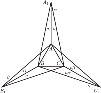
Denote by 𝒢\mathcal{G} the set of subgroups ΓA,ΓB,ΓC,ΓA1,ΓB1,ΓC1\Gamma_{A},\Gamma_{B},\Gamma_{C},\Gamma_{A_{1}},\Gamma_{B_{1}},\Gamma_{C_{1}}, and all their pairwise and triple intersections.

Denote by Ξ\Xi the simplicial complex associated with the poset of the subsets of Γ\Gamma of the form G⋅gG\cdot g for G∈𝒢G\in\mathcal{G} and g∈Γg\in\Gamma. Then Ξ\Xi is a Γ\Gamma-invariant sub-complex of the barycentric subdivision of the Cayley-Rips complex Ξ¯\overline{\Xi} of Γ\Gamma defined by the generating set 𝒩\mathcal{N} (see Subsection 3.5).

Denote by 𝒯0\mathcal{T}_{0} the simplcial complex of the poset 𝒢\mathcal{G}. It is the subcomplex of Ξ\Xi spanned by the vertices corresponding to cosets containing the identity, i.e., it is the union of the simplicies of Ξ\Xi containing the vertex corresponding to the trivial subgroup {ε}∈𝒢\{\varepsilon\}\in\mathcal{G} of Γ\Gamma.

It follows from the description of the set of groups 𝒢\mathcal{G} that we can represent 𝒯0\mathcal{T}_{0} as a union of three tetrahedra A1​A​B​CA_{1}ABC, B1​A​B​CB_{1}ABC, C1​A​B​CC_{1}ABC with a common face A​B​CABC, as it is shown on Figure 5. Every element ΓX\Gamma_{X}, ΓX​Y\Gamma_{XY}, or ΓX​Y​Z\Gamma_{XYZ} of 𝒢\mathcal{G} corresponds to (the barycenter of) the corresponding vertex XX, edge X​YXY, or triangle X​Y​ZXYZ, respectively. We have labeled on Figure 5 the triangles of 𝒯0\mathcal{T}_{0} by the generators of the respective groups ΓX​Y​Z\Gamma_{XYZ}.

Refer to caption
Figure 5. Complex 𝒯0\mathcal{T}_{0} associated with 𝒩\mathcal{N}

Denote

Ξn=Ξ⊗𝔐⊗n,𝒯n=𝒯0⊗𝖷n⊂Ξn.\Xi_{n}=\Xi\otimes\mathfrak{M}^{\otimes n},\quad\mathcal{T}_{n}=\mathcal{T}_{0}\otimes\mathsf{X}^{n}\subset\Xi_{n}.

The set 𝒯n\mathcal{T}_{n} is a fundamental domain of the action of Γ\Gamma on Ξn\Xi_{n} (since 𝖷n=𝖷⊗n\mathsf{X}^{n}=\mathsf{X}^{\otimes n} is a right orbit transversal of the action of Γ\Gamma on 𝔐⊗n\mathfrak{M}^{\otimes n}). The space 𝒯n\mathcal{T}_{n} is the quotient of the space 𝒯0×𝖷n\mathcal{T}_{0}\times\mathsf{X}^{n} by the identifications

(ξ,v)∼(ξ⋅g−1,g⁡(v))(\xi,v)\sim(\xi\cdot g^{-1},g(v))

for all g∈𝒩g\in\mathcal{N}, ξ∈𝒯0\xi\in\mathcal{T}_{0}, and v∈𝖷nv\in\mathsf{X}^{n} such that g|v=εg|_{v}=\varepsilon and ξ⋅g−1∈𝒯0\xi\cdot g^{-1}\in\mathcal{T}_{0}.

We will denote the points of 𝒯n\mathcal{T}_{n} in the same way as the points of Ξn\Xi_{n}: the point ξ⊗v\xi\otimes v is the equivalence class of the point (ξ,v)∈𝒯0×𝖷n(\xi,v)\in\mathcal{T}_{0}\times\mathsf{X}^{n}.

For g∈Γg\in\Gamma, denote Kg,n=𝒯n∩𝒯n⋅gK_{g,n}=\mathcal{T}_{n}\cap\mathcal{T}_{n}\cdot g, and let κg,n:Kg,n→Kg−1,n\kappa_{g,n}:K_{g,n}\rightarrow K_{g^{-1},n} be restriction onto Kg,nK_{g,n} of the map ξ↦ξ⋅g−1\xi\mapsto\xi\cdot g^{-1}.

If 𝒯0∩𝒯0⋅g\mathcal{T}_{0}\cap\mathcal{T}_{0}\cdot g is non-empty for g∈Γg\in\Gamma, then there exists G∈𝒢G\in\mathcal{G} such that G⋅g∈𝒢G\cdot g\in\mathcal{G}. But then g∈G⊂𝒩g\in G\subset\mathcal{N}, and G⋅g=GG\cdot g=G. It follows that Kg,0K_{g,0} is non-empty only for g∈𝒩g\in\mathcal{N}; Kg,0=Kg−1,0K_{g,0}=K_{g^{-1},0}; and κg,0\kappa_{g,0} is an identity map.

We have

Kα,0=A1​B​C,Kβ,0=B1​A​C,Kγ,0=C1​A​B,\displaystyle K_{\alpha,0}=A_{1}BC,\quad K_{\beta,0}=B_{1}AC,\quad K_{\gamma,0}=C_{1}AB,
Ka,0=B1​B​C,Kb,0=A1​A​C,Kc,0=A1​A​B,\displaystyle K_{a,0}=B_{1}BC,\quad K_{b,0}=A_{1}AC,\quad K_{c,0}=A_{1}AB,
Ka​α,0=C1​C​B,Kb​β,0=C1​C​A,Kc​γ,0=B1​B​A.\displaystyle K_{a\alpha,0}=C_{1}CB,\quad K_{b\beta,0}=C_{1}CA,\quad K_{c\gamma,0}=B_{1}BA.

The remaining sets Kg,0K_{g,0} for g∈𝔄g\in\mathfrak{A} are one-dimensional:

Kα​c,0=A1​B,Ka​α​γ,0=C1​B.K_{\alpha c,0}=A_{1}B,\quad K_{a\alpha\gamma,0}=C_{1}B.
Proposition 5.2.

The set Kg,nK_{g,n} is non-empty only for g∈𝒩g\in\mathcal{N}. The map κg,n:Kg,n→Kg−1,n\kappa_{g,n}:K_{g,n}\rightarrow K_{g^{-1},n} is given by the condition

κg,n​(ξ⊗v)=ξ⊗h⁡(v),\kappa_{g,n}(\xi\otimes v)=\xi\otimes h(v),

where h∈𝒩h\in\mathcal{N} is such that h|v=gh|_{v}=g, and ξ∈Kh,0\xi\in K_{h,0}.

Proof.

If κg,n\kappa_{g,n} is defined on a point ξ⊗v\xi\otimes v, for ξ∈𝒯0\xi\in\mathcal{T}_{0} and v∈𝖷nv\in\mathsf{X}^{n}, then ξ⊗v⋅g−1=ξ1⊗v1\xi\otimes v\cdot g^{-1}=\xi_{1}\otimes v_{1} for some ξ1∈𝒯0\xi_{1}\in\mathcal{T}_{0} and v1∈𝖷nv_{1}\in\mathsf{X}^{n}. Then, by the definition of a tensor product, there exists h∈Γh\in\Gamma such that ξ=ξ1⋅h\xi=\xi_{1}\cdot h and h⋅v⋅g−1=v1h\cdot v\cdot g^{-1}=v_{1} in 𝔐⊗n\mathfrak{M}^{\otimes n}. The first equality implies, by the argument above, that h∈𝒩h\in\mathcal{N} and ξ=ξ1∈Kh,0\xi=\xi_{1}\in K_{h,0}. Then v1=h⁡(v)v_{1}=h(v) and h|v⋅g−1=εh|_{v}\cdot g^{-1}=\varepsilon, which implies that g=h|v∈𝒩g=h|_{v}\in\mathcal{N}. ∎

The next technical lemma will be used several times in our paper.

Lemma 5.3.

For every point ξ∈𝒯n\xi\in\mathcal{T}_{n} the stabilizer Γξ\Gamma_{\xi} of ξ\xi in Γ\Gamma belongs either to 𝒢\mathcal{G} or to the set

𝒢1={⟨aαγ,αc⟩,⟨aαγ⟩,⟨αc⟩}.\mathcal{G}_{1}=\left\{\langle a\alpha\gamma,\alpha c\rangle,\quad\langle a\alpha\gamma\rangle,\quad\langle\alpha c\rangle\right\}.

In particular, it is generated by a subset of 𝔄\mathfrak{A}.

If ξ∈𝒯n\xi\in\mathcal{T}_{n} belongs to Kg,nK_{g,n} for g∈𝒩∖𝔄g\in\mathcal{N}\setminus\mathfrak{A}, then κg,n​(ξ)=ξ\kappa_{g,n}(\xi)=\xi, i.e., gg belongs to Γξ\Gamma_{\xi}.

Proof.

We have seen above that stabilizer of every point ξ∈𝒯0\xi\in\mathcal{T}_{0} belongs to 𝒢\mathcal{G}.

Let us prove our lemma by induction. Suppose that it is true for nn, and let gg be an element of the stabilizer of a point ξ⊗v​x\xi\otimes vx for ξ∈𝒯0\xi\in\mathcal{T}_{0}, v∈𝖷nv\in\mathsf{X}^{n}, and x∈𝖷x\in\mathsf{X}. Then ξ⊗v​x⋅g=ξ⊗v​x\xi\otimes vx\cdot g=\xi\otimes vx, which means that there exists h∈Γh\in\Gamma such that ξ⊗v=ξ⊗v⋅h\xi\otimes v=\xi\otimes v\cdot h and h⋅x=x⋅gh\cdot x=x\cdot g. Consequently, elements of the stabilizer of ξ⊗v​x\xi\otimes vx are sections at xx of the intersection of Γξ⊗v\Gamma_{\xi\otimes v} with the stabilizer of xx. In other words

Γξ⊗v​x=ϕx​(Γξ⊗v),\Gamma_{\xi\otimes vx}=\phi_{x}(\Gamma_{\xi\otimes v}),

where ϕx\phi_{x} is the virtual endomorphism associated with Γ\Gamma and x∈𝖷x\in\mathsf{X}.

The generators of G∈𝒢G\in\mathcal{G} (as they are listed in Subsection 5.3) acting non-trivially on the first level belong to {α,a,a​α}\{\alpha,a,a\alpha\}. Consequently, for every g∈Gg\in G and x∈𝖷x\in\mathsf{X} the section g|xg|_{x} is equal to ϕx​(h)\phi_{x}(h) for some h∈Gh\in G. Therefore, ϕx​(G)=G|x\phi_{x}(G)=G|_{x} for all G∈𝒢G\in\mathcal{G}. The groups G|xG|_{x} are listed in Subsection 5.4 (one has also to add the sections ⟨g⟩|x=⟨g|x⟩\langle g\rangle|_{x}=\langle g|_{x}\rangle for g∈𝔄g\in\mathfrak{A}).

We see that G|x∈𝒢∪𝒢1G|_{x}\in\mathcal{G}\cup\mathcal{G}_{1} for all G∈𝒢G\in\mathcal{G}. Sections g|xg|_{x} of the elements of the groups from 𝒢1\mathcal{G}_{1} belong to ⟨β,b⟩\langle\beta,b\rangle. But all subgroups of ⟨β,b⟩\langle\beta,b\rangle belong to 𝒢\mathcal{G}. It follows that stabilizers of points of 𝒯n\mathcal{T}_{n} belong to 𝒢∪𝒢1\mathcal{G}\cup\mathcal{G}_{1} for all nn.

Let us prove the remaining part of the lemma. Let ξ∈𝒯0\xi\in\mathcal{T}_{0}, v∈𝖷nv\in\mathsf{X}^{n}, and x∈𝖷x\in\mathsf{X} are such that ξ⊗v​x\xi\otimes vx belongs to Kg,n+1K_{g,n+1} for g∈𝒩∖𝔄g\in\mathcal{N}\setminus\mathfrak{A}. Then there exists h∈𝒩h\in\mathcal{N} such that ξ⋅h=ξ\xi\cdot h=\xi and h|v​x=gh|_{vx}=g. Since 𝔄\mathfrak{A} is state-closed, h|v∉𝔄h|_{v}\notin\mathfrak{A}. We have then ξ⊗v=ξ⊗h⋅v=ξ⊗h⁡(v)⋅h|v\xi\otimes v=\xi\otimes h\cdot v=\xi\otimes h(v)\cdot h|_{v}, i.e., ξ⊗v∈Kh|v,n\xi\otimes v\in K_{h|_{v},n}. By the inductive assumption, h|vh|_{v} belongs to the stabilizer of ξ⊗v\xi\otimes v.

Consequently, ξ⊗h⁡(v)=ξ⊗v⋅h|v−1=ξ⊗v\xi\otimes h(v)=\xi\otimes v\cdot h|_{v}^{-1}=\xi\otimes v. It follows that there exists h′∈𝒩h^{\prime}\in\mathcal{N} such that ξ⋅h′=ξ\xi\cdot h^{\prime}=\xi, h′​h​(v)=vh^{\prime}h(v)=v, and h′|h⁡(v)=εh^{\prime}|_{h(v)}=\varepsilon. We have then for h1=h​h′h_{1}=hh^{\prime}:

ξ⋅h1=ξ,h1⋅v=h′​h⋅v=v⋅h′|h⁡(v)​h|v=v⋅h|v.\xi\cdot h_{1}=\xi,\qquad h_{1}\cdot v=h^{\prime}h\cdot v=v\cdot h^{\prime}|_{h(v)}h|_{v}=v\cdot h|_{v}.

We may assume therefore that h⁡(v)=vh(v)=v.

Note that h|vh|_{v} can not belong to any of the groups of the set 𝒢1\mathcal{G}_{1}, since then g=h|v​x∈⟨β,b⟩⊂𝔄g=h|_{vx}\in\langle\beta,b\rangle\subset\mathfrak{A}. Consequently, h|vh|_{v} belongs to one of the groups of the set 𝒢\mathcal{G}.

If h|v​(x)=xh|_{v}(x)=x, then ξ⊗v​x=ξ⊗h⋅v​x=ξ⊗v​x⋅g\xi\otimes vx=\xi\otimes h\cdot vx=\xi\otimes vx\cdot g, and gg belongs to the stabilizer of ξ⊗v​x\xi\otimes vx.

Suppose that h|v​(x)≠xh|_{v}(x)\neq x. All the generators of the groups in the set 𝒢\mathcal{G} acting non-trivially on the first level belong to the set {α,a,α​a}\{\alpha,a,\alpha a\} of elements having trivial sections. Consequently, if h|vh|_{v} belongs to one of the stabilizers from 𝒢\mathcal{G}, then h|v​(x)=δ​(x)h|_{v}(x)=\delta(x) for δ∈{α,a,α​a}\delta\in\{\alpha,a,\alpha a\}, and ξ⊗v​x=ξ⊗v⋅δ⊗x=ξ⊗v​h|v​(x)\xi\otimes vx=\xi\otimes v\cdot\delta\otimes x=\xi\otimes vh|_{v}(x), therefore gg belongs to the stabilizer of ξ⊗v​x\xi\otimes vx. ∎

Let us describe now a recursive procedure of constructing the complexes 𝒯n\mathcal{T}_{n}.

Theorem 5.4.

The space 𝒯n+1\mathcal{T}_{n+1} is the quotient of the space 𝒯n×𝖷\mathcal{T}_{n}\times\mathsf{X} by the equivalence relation generated by the identifications

ξ⊗x=κg,n​(ξ)⊗g⁡(x)\xi\otimes x=\kappa_{g,n}(\xi)\otimes g(x)

for all g∈𝔄g\in\mathfrak{A}, x∈𝖷x\in\mathsf{X}, ξ∈Kg,n\xi\in K_{g,n}, such that g|x=εg|_{x}=\varepsilon.

The set Kg,n+1K_{g,n+1} for g∈𝔄g\in\mathfrak{A} is equal to

⋃h∈𝔄,x∈𝖷,h|x=gKh,n⊗x.\bigcup_{h\in\mathfrak{A},x\in\mathsf{X},h|_{x}=g}K_{h,n}\otimes x.

The map κg,n+1:Kg,n+1→Kg,n+1\kappa_{g,n+1}:K_{g,n+1}\rightarrow K_{g,n+1} for g∈𝔄g\in\mathfrak{A} acts by the rule

κg,n+1​(ξ⊗x)=κh,n​(ξ)⊗h⁡(x),\kappa_{g,n+1}(\xi\otimes x)=\kappa_{h,n}(\xi)\otimes h(x),

where h∈𝔄h\in\mathfrak{A} is such that h|x=gh|_{x}=g, and ξ∈Kh,n\xi\in K_{h,n}.

All the information used in the inductive pasting rule of Theorem 5.4 is read directly from the wreath recursion (4)–(8) (Subsection 5.1) or from the structure of the automaton 𝔄\mathfrak{A} on Figure 4.

For instance, the identification of the copies 𝒯n×x\mathcal{T}_{n}\times x of 𝒯n\mathcal{T}_{n} are given by the maps:

(κα,n,σ)\displaystyle(\kappa_{\alpha,n},\sigma) :\displaystyle: Kα,n×𝖷→Kα,n×𝖷,\displaystyle K_{\alpha,n}\times\mathsf{X}\rightarrow K_{\alpha,n}\times\mathsf{X},
(κa,n,π)\displaystyle(\kappa_{a,n},\pi) :\displaystyle: Ka,n×𝖷→Ka,n×𝖷,\displaystyle K_{a,n}\times\mathsf{X}\rightarrow K_{a,n}\times\mathsf{X},
(κa​α,n,π​σ)\displaystyle(\kappa_{a\alpha,n},\pi\sigma) :\displaystyle: Ka​α,n×𝖷→Ka​α,n×𝖷,\displaystyle K_{a\alpha,n}\times\mathsf{X}\rightarrow K_{a\alpha,n}\times\mathsf{X},

and

(κγ,n,ε)\displaystyle(\kappa_{\gamma,n},\varepsilon) :\displaystyle: Kγ,n×{2,3}→Kγ,n×{2,3},\displaystyle K_{\gamma,n}\times\{\mathit{2},\mathit{3}\}\rightarrow K_{\gamma,n}\times\{\mathit{2},\mathit{3}\},
(κa​α​γ,n,π​σ):\displaystyle(\kappa_{a\alpha\gamma,n},\pi\sigma): :\displaystyle: Ka​α​γ,n×{2,3}→Ka​α​γ,n×{2,3}.\displaystyle K_{a\alpha\gamma,n}\times\{\mathit{2},\mathit{3}\}\rightarrow K_{a\alpha\gamma,n}\times\{\mathit{2},\mathit{3}\}.
Proof.

If we replace 𝔄\mathfrak{A} by 𝒩\mathcal{N} everywhere in the theorem, then it will follow directly from the definition of the tensor product Ξn+1=Ξn⊗𝔐\Xi_{n+1}=\Xi_{n}\otimes\mathfrak{M}.

Therefore, the space 𝒯n+1\mathcal{T}_{n+1} is obtained by taking the quotient of the space 𝒯n×𝖷\mathcal{T}_{n}\times\mathsf{X} by the identifications

(9) (ξ,x)∼(κg,n​(ξ),g⁡(x)),(\xi,x)\sim(\kappa_{g,n}(\xi),g(x)),

where g∈𝒩g\in\mathcal{N}, g|x=εg|_{x}=\varepsilon, and ξ∈Kg,n\xi\in K_{g,n}. Suppose that gg does not belong to 𝔄\mathfrak{A}. Then, by Lemma 5.3, gg belongs to the stabilizer Γξ\Gamma_{\xi} of ξ\xi, and Γξ∈𝒢∪𝒢1\Gamma_{\xi}\in\mathcal{G}\cup\mathcal{G}_{1}. Identification (9) becomes (ξ,x)∼(ξ,g⁡(x))(\xi,x)\sim(\xi,g(x)). If x=g⁡(x)x=g(x), the identification is trivial. If g⁡(x)≠xg(x)\neq x and gg is an element of one of the groups in the set 𝒢\mathcal{G}, then there exists δ∈{α,a,α​a}\delta\in\{\alpha,a,\alpha a\} such that ξ⋅δ=ξ\xi\cdot\delta=\xi and δ⁡(x)=g⁡(x)\delta(x)=g(x). Then identification (9) is made using elements of 𝔄\mathfrak{A}. If gg is an element of a group from the set 𝒢1\mathcal{G}_{1}, then either g∈𝔄g\in\mathfrak{A}, or g∈{a​α​γ​α​c,a​c}g\in\{a\alpha\gamma\alpha c,ac\}. But a​α​γ​α​c=π⁡(b​β,b,b​β,b)a\alpha\gamma\alpha c=\pi(b\beta,b,b\beta,b) and a​c=π⁡(b​β,b​β,b,b)ac=\pi(b\beta,b\beta,b,b), which contradicts the condition g|x=εg|_{x}=\varepsilon. We see that identification (9) is either trivial, or can implemented by an element of 𝔄\mathfrak{A}.

It remains to prove that every point of Kg,n+1K_{g,n+1} for g∈𝔄g\in\mathfrak{A} can be represented by ξ⊗x\xi\otimes x for ξ∈Kh,n\xi\in K_{h,n} and x∈𝖷x\in\mathsf{X}, where h∈𝔄h\in\mathfrak{A} is such that h|x=gh|_{x}=g.

Every point of Kg,n+1K_{g,n+1} can be written as ξ⊗x\xi\otimes x for ξ∈Kh0,n\xi\in K_{h_{0},n} and x∈𝖷x\in\mathsf{X}, where h0∈𝒩h_{0}\in\mathcal{N} is such that h0|x=gh_{0}|_{x}=g. Suppose that h0∉𝔄h_{0}\notin\mathfrak{A}. Then, by Lemma 5.3, h0h_{0} belongs to the stabilizer Γξ∈𝒢∪𝒢1\Gamma_{\xi}\in\mathcal{G}\cup\mathcal{G}_{1}. It is enough then to show that there exist h∈Γξ∩𝔄h\in\Gamma_{\xi}\cap\mathfrak{A} and y∈𝖷y\in\mathsf{X} such that ξ⊗x=ξ⊗y\xi\otimes x=\xi\otimes y and h|y=gh|_{y}=g. We have ξ⊗x=ξ⊗y\xi\otimes x=\xi\otimes y if there exists δ∈Γξ\delta\in\Gamma_{\xi} such that δ⋅x=y⋅ε\delta\cdot x=y\cdot\varepsilon.

Thus, theorem is proved if we show that for all G∈𝒢∪𝒢1G\in\mathcal{G}\cup\mathcal{G}_{1}, x∈𝖷x\in\mathsf{X}, and g∈G|x∩𝔄g\in G|_{x}\cap\mathfrak{A} there exists δ∈G\delta\in G and h∈G∩𝔄h\in G\cap\mathfrak{A} such that δ|x=ε\delta|_{x}=\varepsilon and h|δ⁡(x)=gh|_{\delta(x)}=g.

Let us consider all the cases. If G=ΓA=⟨β,γ,b,c⟩G=\Gamma_{A}=\langle\beta,\gamma,b,c\rangle, then for every x∈𝖷x\in\mathsf{X} and g∈G|x∩𝔄g\in G|_{x}\cap\mathfrak{A} there exists h∈Gh\in G such that h|x=gh|_{x}=g (so we can take δ=ε\delta=\varepsilon):

  1. (1)

    For x=1x=\mathit{1}, G|1∩𝔄={ε,α,β,a,b,a​α,b​β}G|_{\mathit{1}}\cap\mathfrak{A}=\{\varepsilon,\alpha,\beta,a,b,a\alpha,b\beta\}, and

    α=β|1,β=γ|1,a=(b​β)|1,b=(c​γ)|1,a​α=b|1,b​β=c|1.\alpha=\beta|_{\mathit{1}},\quad\beta=\gamma|_{\mathit{1}},\quad a=(b\beta)|_{\mathit{1}},\quad b=(c\gamma)|_{\mathit{1}},\quad a\alpha=b|_{\mathit{1}},\quad b\beta=c|_{\mathit{1}}.
  2. (2)

    For x=2x=\mathit{2}, G|2∩𝔄={ε,γ,a​α,b​β,a​α​γ}G|_{\mathit{2}}\cap\mathfrak{A}=\{\varepsilon,\gamma,a\alpha,b\beta,a\alpha\gamma\}, and

    γ=β|2,a​α=b|2,b​β=c|2,a​α​γ=(b​β)|2.\gamma=\beta|_{\mathit{2}},\quad a\alpha=b|_{\mathit{2}},\quad b\beta=c|_{\mathit{2}},\quad a\alpha\gamma=(b\beta)|_{\mathit{2}}.
  3. (3)

    For x=3x=\mathit{3}, G|3∩𝔄={ε,α,b,c,α​c}G|_{\mathit{3}}\cap\mathfrak{A}=\{\varepsilon,\alpha,b,c,\alpha c\}, and

    α=β|3,b=c|3,c=b|3,α​c=(b​β)|3.\alpha=\beta|_{\mathit{3}},\quad b=c|_{\mathit{3}},\quad c=b|_{\mathit{3}},\quad\alpha c=(b\beta)|_{\mathit{3}}.
  4. (4)

    For x=4x=\mathit{4}, G|4∩𝔄={ε,β,γ,b,c,b​β,c​γ}G|_{\mathit{4}}\cap\mathfrak{A}=\{\varepsilon,\beta,\gamma,b,c,b\beta,c\gamma\}, and

    β=γ|4,γ=β|4,b=c|4,c=b|4,b​β=(c​γ)|4,c​γ=(b​β)|4.\beta=\gamma|_{\mathit{4}},\quad\gamma=\beta|_{\mathit{4}},\quad b=c|_{\mathit{4}},\quad c=b|_{\mathit{4}},\quad b\beta=(c\gamma)|_{\mathit{4}},\quad c\gamma=(b\beta)|_{\mathit{4}}.

If G=ΓB=⟨α,γ,a,c⟩G=\Gamma_{B}=\langle\alpha,\gamma,a,c\rangle, then G|x=⟨β,b⟩G|_{x}=\langle\beta,b\rangle for all x∈𝖷x\in\mathsf{X}. For any pair x,y∈𝖷x,y\in\mathsf{X} there exists δ∈⟨α,a⟩⊂ΓB\delta\in\langle\alpha,a\rangle\subset\Gamma_{B} such that δ⁡(x)=y\delta(x)=y. Hence, equalities

β=γ|1,b=c|1,b​β=(c​γ)|1,\beta=\gamma|_{\mathit{1}},\quad b=c|_{\mathit{1}},\quad b\beta=(c\gamma)|_{\mathit{1}},

finish the proof for G=ΓBG=\Gamma_{B}.

The case G=ΓC=⟨α,β,a,b⟩G=\Gamma_{C}=\langle\alpha,\beta,a,b\rangle is considered in the same way. We have G|x=⟨α,γ,a,c⟩G|_{x}=\langle\alpha,\gamma,a,c\rangle for all x∈𝖷x\in\mathsf{X}, and

α=β|1,a=(b​β)|1,a​α=b|1,\displaystyle\alpha=\beta|_{\mathit{1}},\quad a=(b\beta)|_{\mathit{1}},\quad a\alpha=b|_{\mathit{1}},
γ=β|2,c=b|3,c​γ=(b​β)|4,\displaystyle\gamma=\beta|_{\mathit{2}},\quad c=b|_{\mathit{3}},\quad c\gamma=(b\beta)|_{\mathit{4}},
α​c=(b​β)|3,a​α​γ=(b​β)|2.\displaystyle\alpha c=(b\beta)|_{\mathit{3}},\quad a\alpha\gamma=(b\beta)|_{\mathit{2}}.

Consider the case G=ΓA1=⟨α,b,c⟩G=\Gamma_{A_{1}}=\langle\alpha,b,c\rangle. If x∈{1,2}x\in\{\mathit{1},\mathit{2}\}, then G|x∩𝔄={ε,a​α,b​β}G|_{x}\cap\mathfrak{A}=\{\varepsilon,a\alpha,b\beta\}, and

a​α=b|x,b​β=c|x.a\alpha=b|_{x},\quad b\beta=c|_{x}.

If x∈{3,4}x\in\{\mathit{3},\mathit{4}\}, then G|x∩𝔄={ε,b,c}G|_{x}\cap\mathfrak{A}=\{\varepsilon,b,c\} and

b=c|x,c=b|x.b=c|_{x},\quad c=b|_{x}.

Cases G=ΓB1G=\Gamma_{B_{1}} and G=ΓC1G=\Gamma_{C_{1}} are similar to ΓA1\Gamma_{A_{1}}.

Cases G∈{ΓA​B,ΓA​C,ΓA​A1,ΓA​B1,ΓA​C1}G\in\{\Gamma_{AB},\Gamma_{AC},\Gamma_{AA_{1}},\Gamma_{AB_{1}},\Gamma_{AC_{1}}\} are straightforward: GG acts trivially on the first level; G|x∩𝔄G|_{x}\cap\mathfrak{A} coincides with the standard generating set; and for every x∈𝖷x\in\mathsf{X}, g∈G|x∩𝔄g\in G|_{x}\cap\mathfrak{A} there exists h∈G∩𝔄h\in G\cap\mathfrak{A} such that h|x=gh|_{x}=g.

There is nothing to prove for G=ΓB​CG=\Gamma_{BC}.

Cases G∈{ΓB​A1,ΓB​B1,ΓB​C1,ΓC​A1,ΓC​B1,ΓC​C1}G\in\{\Gamma_{BA_{1}},\Gamma_{BB_{1}},\Gamma_{BC_{1}},\Gamma_{CA_{1}},\Gamma_{CB_{1}},\Gamma_{CC_{1}}\} are similar to G=ΓA1G=\Gamma_{A_{1}}: the group GG contains an element δ∈{α,a,a​α}\delta\in\{\alpha,a,a\alpha\}; intersection of G|xG|_{x} with 𝔄\mathfrak{A} is the standard generating set of G|xG|_{x}; for every x∈𝖷x\in\mathsf{X} and g∈G|x∩𝔄g\in G|_{x}\cap\mathfrak{A} there exists h∈G∩𝔄h\in G\cap\mathfrak{A} such that either h|x=gh|_{x}=g, or h|δ⁡(x)=gh|_{\delta(x)}=g.

If G=⟨g⟩∈𝒢∪𝒢1G=\langle g\rangle\in\mathcal{G}\cup\mathcal{G}_{1} is cyclic, then g,g|x∈𝔄g,g|_{x}\in\mathfrak{A}, and we are done.

The only remaining case is G=⟨a​α​γ,α​c⟩G=\langle a\alpha\gamma,\alpha c\rangle. Since a​α​γ⋅α​c=π⁡(b​β,b,b​β,b)=γ​a​ca\alpha\gamma\cdot\alpha c=\pi(b\beta,b,b\beta,b)=\gamma ac is an involution, we have

G={ε,aαγ=πσ(β,ε,ε,β),αc=σ(bβ,bβ,b,b),γac=π(bβ,b,bβ,b)},G=\{\varepsilon,\quad a\alpha\gamma=\pi\sigma(\beta,\varepsilon,\varepsilon,\beta),\quad\alpha c=\sigma(b\beta,b\beta,b,b),\quad\gamma ac=\pi(b\beta,b,b\beta,b)\},

hence

G|1={ε,β=(a​α​γ)|1,b​β=(α​c)|1},G|4={ε,β=(a​α​γ)|4,b=(α​c)|4}.G|_{\mathit{1}}=\{\varepsilon,\beta=(a\alpha\gamma)|_{\mathit{1}},b\beta=(\alpha c)|_{\mathit{1}}\},\quad G|_{\mathit{4}}=\{\varepsilon,\beta=(a\alpha\gamma)|_{\mathit{4}},b=(\alpha c)|_{\mathit{4}}\}.

We also have a​α​γ⋅2=3⋅εa\alpha\gamma\cdot\mathit{2}=\mathit{3}\cdot\varepsilon, a​α​γ⋅3=2⋅εa\alpha\gamma\cdot\mathit{3}=\mathit{2}\cdot\varepsilon, and

G|2=G|3={ε,b=(α​c)|2,b=(α​c)|3},G|_{\mathit{2}}=G|_{\mathit{3}}=\{\varepsilon,b=(\alpha c)|_{\mathit{2}},b=(\alpha c)|_{\mathit{3}}\},

which finishes the proof. ∎

5.6. Equivariant map

Let us construct the complex 𝒯1\mathcal{T}_{1}. By Theorem 5.4, it is obtained by gluing four copies 𝒯0⊗x\mathcal{T}_{0}\otimes x, for x=1,2,3,4x=\mathit{1},\mathit{2},\mathit{3},\mathit{4}, of 𝒯0=ℳ\mathcal{T}_{0}=\mathcal{M} along the following faces:

(κα,0,σ):A1​B​C×1\displaystyle(\kappa_{\alpha,0},\sigma):A_{1}BC\times\mathit{1} ∼A1​B​C×2,\displaystyle\sim A_{1}BC\times\mathit{2}, A1​B​C×3\displaystyle\quad A_{1}BC\times\mathit{3} ∼A1​B​C×4,\displaystyle\sim A_{1}BC\times\mathit{4},
(κa,0,π):B1​B​C×1\displaystyle(\kappa_{a,0},\pi):B_{1}BC\times\mathit{1} ∼B1​B​C×3,\displaystyle\sim B_{1}BC\times\mathit{3}, B1​B​C×2\displaystyle\quad B_{1}BC\times\mathit{2} ∼B1​B​C×4,\displaystyle\sim B_{1}BC\times\mathit{4},
(κa​α,0,π​σ):C1​B​C×1\displaystyle(\kappa_{a\alpha,0},\pi\sigma):C_{1}BC\times\mathit{1} ∼C1​B​C×4,\displaystyle\sim C_{1}BC\times\mathit{4}, C1​B​C×2\displaystyle\quad C_{1}BC\times\mathit{2} ∼C1​B​C×3,\displaystyle\sim C_{1}BC\times\mathit{3},

where in each case the identification is identical on the first coordinate. Note that the identification (κa​α​γ,0,π​σ)(\kappa_{a\alpha\gamma,0},\pi\sigma) of C1​B×2C_{1}B\times\mathit{2} with C1​B×3C_{1}B\times\mathit{3} follows from the identification of C1​B​C×2C_{1}BC\times\mathit{2} with C1​B​C×3C_{1}BC\times\mathit{3}. The identification (κγ,0,ε)(\kappa_{\gamma,0},\varepsilon) is trivial.

The resulting complex 𝒯1\mathcal{T}_{1} consists of a square pyramid and two tetrahedra such that one face of each tetrahedron is attached to a diagonal of the square pyramid (see Figure 7, but ignore the labels of the vertices this time). Figure 6 shows the parts 𝒯0⊗i\mathcal{T}_{0}\otimes i of 𝒯1\mathcal{T}_{1} (the vertices of each part 𝒯0⊗i\mathcal{T}_{0}\otimes i are labeled as in 𝒯0\mathcal{T}_{0}).

The map ξ⊗x↦ξ\xi\otimes x\mapsto\xi folds the square pyramid in four using reflections with respect to the planes passing through the point C⊗1=C⊗2=C⊗3=C⊗4C\otimes\mathit{1}=C\otimes\mathit{2}=C\otimes\mathit{3}=C\otimes\mathit{4} and through midpoints of two opposite sides of the base of the pyramid, and folds the two tetrahedra along the planes passing through the images of C1⊗iC_{1}\otimes i and the hight of the pyramid.

Refer to caption
Figure 6. Pasting together 𝒯1\mathcal{T}_{1}

The elements of 𝔄\mathfrak{A} acting non-trivially on the first level are α,a,a​α,α​c\alpha,a,a\alpha,\alpha c, and a​α​γa\alpha\gamma. The first three elements have only trivial sections, hence they produce only the identifications of the copies of 𝒯0\mathcal{T}_{0} and no maps κg,1\kappa_{g,1}.

The element α​c=σ⁡(b​β,b​β,b,b)\alpha c=\sigma(b\beta,b\beta,b,b) produces a part of the map κb​β,1\kappa_{b\beta,1} switching Kα​c,0×1K_{\alpha c,0}\times\mathit{1} with Kα​c,0×2K_{\alpha c,0}\times\mathit{2} and a part of κb,1\kappa_{b,1} switching Kα​c,0×3K_{\alpha c,0}\times\mathit{3} with Kα​c,0×4K_{\alpha c,0}\times\mathit{4}. But Kα​c,0K_{\alpha c,0} is the segment A1​BA_{1}B, for which we have identifications A1​B×1∼A1​B×2A_{1}B\times\mathit{1}\sim A_{1}B\times\mathit{2} and A1​B×3∼A1​B×4A_{1}B\times\mathit{3}\sim A_{1}B\times\mathit{4} as parts of the identifications A1​B​C×i∼A1​B​C×σ⁡(i)A_{1}BC\times i\sim A_{1}BC\times\sigma(i).

The element a​α​γ=π​σ​(β,ε,ε,β)a\alpha\gamma=\pi\sigma(\beta,\varepsilon,\varepsilon,\beta) produces a part of the map κβ,1\kappa_{\beta,1} switching Ka​α​γ,0×1=C1​B×1K_{a\alpha\gamma,0}\times\mathit{1}=C_{1}B\times\mathit{1} with Ka​α​γ,0×3=C1​B×3K_{a\alpha\gamma,0}\times\mathit{3}=C_{1}B\times\mathit{3}. But these sets are also identified in 𝒯1\mathcal{T}_{1}.

We see that all the maps κg,1\kappa_{g,1} are identical. Their domains are

Kα,1=B1​A​C⊗{1,3},Kβ,1=C1​A​B⊗{1,4},Kγ,1=B1​A​C⊗{2,4}\displaystyle K_{\alpha,1}=B_{1}AC\otimes\{\mathit{1},\mathit{3}\},\quad K_{\beta,1}=C_{1}AB\otimes\{\mathit{1},\mathit{4}\},\quad K_{\gamma,1}=B_{1}AC\otimes\{\mathit{2},\mathit{4}\}
Ka,1=C1​C​A⊗1,Kc,1=A1​A​C⊗{3,4},\displaystyle K_{a,1}=C_{1}CA\otimes\mathit{1},\quad K_{c,1}=A_{1}AC\otimes\{\mathit{3},\mathit{4}\},
Kb,1=A1​A​B⊗{3,4}∪B1​B​A⊗{1,3},\displaystyle K_{b,1}=A_{1}AB\otimes\{\mathit{3},\mathit{4}\}\cup B_{1}BA\otimes\{\mathit{1},\mathit{3}\},
Ka​α,1=A1​A​C⊗{1,2},Kc​γ,1=C1​C​A⊗4\displaystyle K_{a\alpha,1}=A_{1}AC\otimes\{\mathit{1},\mathit{2}\},\quad K_{c\gamma,1}=C_{1}CA\otimes\mathit{4}
Kb​β,1=A1​A​B⊗{1,2}∪B1​B​A⊗{2,4},\displaystyle K_{b\beta,1}=A_{1}AB\otimes\{\mathit{1},\mathit{2}\}\cup B_{1}BA\otimes\{\mathit{2},\mathit{4}\},
Ka​α​γ,1=C1​C​A⊗2,Kα​c,1=C1​C​A⊗3.\displaystyle K_{a\alpha\gamma,1}=C_{1}CA\otimes\mathit{2},\quad K_{\alpha c,1}=C_{1}CA\otimes\mathit{3}.

We have seen in Subsection 5.4 that for every G∈𝒢G\in\mathcal{G} and every x∈𝖷x\in\mathsf{X} there exists H∈𝒢H\in\mathcal{G} such that G|x⊆HG|_{x}\subseteq H.

For G∈{ΓA,ΓB,ΓC,ΓA1,ΓB1,ΓC1}G\in\{\Gamma_{A},\Gamma_{B},\Gamma_{C},\Gamma_{A_{1}},\Gamma_{B_{1}},\Gamma_{C_{1}}\} and for x∈𝖷x\in\mathsf{X} denote by I⁡(G,x)I(G,x) the intersection of the groups H∈𝒢H\in\mathcal{G} for which G|x⊆HG|_{x}\subseteq H.

Denote for G∈{ΓA,ΓB,ΓC,ΓA1,ΓB1,ΓC1}G\in\{\Gamma_{A},\Gamma_{B},\Gamma_{C},\Gamma_{A_{1}},\Gamma_{B_{1}},\Gamma_{C_{1}}\} and g∈Γg\in\Gamma:

I⁡(G⋅g,x)=I⁡(G,g⁡(x))⋅g|x.I(G\cdot g,x)=I(G,g(x))\cdot g|_{x}.

Then I⁡(G⋅g,x)I(G\cdot g,x) is the intersection of the cosets H⋅hH\cdot h, for H∈𝒢H\in\mathcal{G} and h∈Γh\in\Gamma, containing the set (G⋅g)|x(G\cdot g)|_{x}. The maps I⁡(⋅,x)I(\cdot,x) satisfy the condition

I⁡(U⋅g,x)=I⁡(U,g⁡(x))⋅g|x,I(U\cdot g,x)=I(U,g(x))\cdot g|_{x},

for all cosets UU and for all g∈Γg\in\Gamma, x∈𝖷x\in\mathsf{X}.

Recall that Ξ=⋃g∈Γ𝒯0⋅g\Xi=\bigcup_{g\in\Gamma}\mathcal{T}_{0}\cdot g, where 𝒯0\mathcal{T}_{0} is a union of three tetrahedra A1​A​B​CA_{1}ABC, B1​A​B​CB_{1}ABC, C1​A​B​CC_{1}ABC with vertices corresponding to the groups ΓA\Gamma_{A}, ΓB\Gamma_{B}, ΓC\Gamma_{C}, ΓA1\Gamma_{A_{1}}, ΓB1\Gamma_{B_{1}}, and ΓC1\Gamma_{C_{1}}. It is checked directly that for every x∈𝖷x\in\mathsf{X} the image of the set of vertices of each of these tetrahedra under I⁡(⋅,x)I(\cdot,x) is a subset of one of the tetrahedra (we will see this also in the geometric description of the maps I⁡(⋅,x)I(\cdot,x) below). Consequently, we can extend I⁡(⋅,x)I(\cdot,x) by linearity to the whole complex Ξ\Xi. In this way we get continuous maps satisfying the condition

I⁡(ξ⋅g,x)=I⁡(ξ,g⁡(x))⋅g|x,I(\xi\cdot g,x)=I(\xi,g(x))\cdot g|_{x},

for all ξ∈Ξ\xi\in\Xi, g∈Γg\in\Gamma, and x∈𝖷x\in\mathsf{X}. Hence, the map I⁡(ξ⊗x)=I⁡(ξ,x)I(\xi\otimes x)=I(\xi,x) is a well defined continuous equivariant map from Ξ1=Ξ⊗𝔐\Xi_{1}=\Xi\otimes\mathfrak{M} to Ξ\Xi.

Figure 7 shows the complex 𝒯1\mathcal{T}_{1} in the same way as it is shown on Figure 6, but with vertices labeled by their images under the map II (except for B1′B_{1}^{\prime}, which is mapped to BB). One tetrahedron (B1′​A1​B​C1B_{1}^{\prime}A_{1}BC_{1} on Figure 7) is collapsed by II onto the diagonal of the square pyramid (triangle A1​B​C1A_{1}BC_{1}). The remaining part of 𝒯1\mathcal{T}_{1} is a union of three tetrahedra and is mapped by a locally affine homeomorphism onto 𝒯0\mathcal{T}_{0}.

Refer to caption
Figure 7. The complex 𝒯1\mathcal{T}_{1}

We have the following formulae for II (see Figures 5):

I⁡(A⊗1)\displaystyle I(A\otimes\mathit{1}) =C,\displaystyle=C, I⁡(B⊗1)\displaystyle\quad I(B\otimes\mathit{1}) =(A​C),\displaystyle=(AC), I⁡(C⊗1)\displaystyle\quad I(C\otimes\mathit{1}) =B,\displaystyle=B,
I⁡(A⊗2)\displaystyle I(A\otimes\mathit{2}) =C1,\displaystyle=C_{1}, I⁡(B⊗2)\displaystyle\quad I(B\otimes\mathit{2}) =(A​C),\displaystyle=(AC), I⁡(C⊗2)\displaystyle\quad I(C\otimes\mathit{2}) =B,\displaystyle=B,
I⁡(A⊗3)\displaystyle I(A\otimes\mathit{3}) =A1,\displaystyle=A_{1}, I⁡(B⊗3)\displaystyle\quad I(B\otimes\mathit{3}) =(A​C),\displaystyle=(AC), I⁡(C⊗3)\displaystyle\quad I(C\otimes\mathit{3}) =B,\displaystyle=B,
I⁡(A⊗4)\displaystyle I(A\otimes\mathit{4}) =A,\displaystyle=A, I⁡(B⊗4)\displaystyle\quad I(B\otimes\mathit{4}) =(A​C),\displaystyle=(AC), I⁡(C⊗4)\displaystyle\quad I(C\otimes\mathit{4}) =B,\displaystyle=B,

and

I⁡(A1⊗1)\displaystyle I(A_{1}\otimes\mathit{1}) =(C​C1),\displaystyle=(CC_{1}), I⁡(B1⊗1)\displaystyle\quad I(B_{1}\otimes\mathit{1}) =(C​A1),\displaystyle=(CA_{1}), I⁡(C1⊗1)\displaystyle\quad I(C_{1}\otimes\mathit{1}) =B1,\displaystyle=B_{1},
I⁡(A1⊗2)\displaystyle I(A_{1}\otimes\mathit{2}) =(C​C1),\displaystyle=(CC_{1}), I⁡(B1⊗2)\displaystyle\quad I(B_{1}\otimes\mathit{2}) =(A​C1),\displaystyle=(AC_{1}), I⁡(C1⊗2)\displaystyle\quad I(C_{1}\otimes\mathit{2}) =B,\displaystyle=B,
I⁡(A1⊗3)\displaystyle I(A_{1}\otimes\mathit{3}) =(A​A1),\displaystyle=(AA_{1}), I⁡(B1⊗3)\displaystyle\quad I(B_{1}\otimes\mathit{3}) =(C​A1),\displaystyle=(CA_{1}), I⁡(C1⊗3)\displaystyle\quad I(C_{1}\otimes\mathit{3}) =B,\displaystyle=B,
I⁡(A1⊗4)\displaystyle I(A_{1}\otimes\mathit{4}) =(A​A1),\displaystyle=(AA_{1}), I⁡(B1⊗4)\displaystyle\quad I(B_{1}\otimes\mathit{4}) =(A​C1),\displaystyle=(AC_{1}), I⁡(C1⊗4)\displaystyle\quad I(C_{1}\otimes\mathit{4}) =B1,\displaystyle=B_{1},

where (X​Y)(XY) denotes the midpoint of the segment X​YXY. The vertices X⊗iX\otimes i are shown on Figure 6: a vertex X⊗iX\otimes i is labeled by XX on the part showing 𝒯0⊗i\mathcal{T}_{0}\otimes i.

The map I:Ξ⊗𝔐→ΞI:\Xi\otimes\mathfrak{M}\rightarrow\Xi is uniquely determined by its restriction I:𝒯1→𝒯0I:\mathcal{T}_{1}\rightarrow\mathcal{T}_{0} onto the fundamental domain, due to equivariance.

Let us introduce a Euclidean structure on the complex Ξ\Xi by embedding the complex 𝒯0\mathcal{T}_{0} into ℝ5\mathbb{R}^{5} in such a way that

{B​A→,B​C→,A​A1→,B​B1→,C​C1→}\{\overrightarrow{BA},\quad\overrightarrow{BC},\quad\overrightarrow{AA_{1}},\quad\overrightarrow{BB_{1}},\quad\overrightarrow{CC_{1}}\}

is the standard orthonormal basis of ℝ6\mathbb{R}^{6}.

Proposition 5.5.

The map I:Ξ⊗𝔐→ΞI:\Xi\otimes\mathfrak{M}\rightarrow\Xi is contracting.

Proof.

The map ξ↦I⁡(ξ⊗x)\xi\mapsto I(\xi\otimes x) is affine on 𝒯0\mathcal{T}_{0} for every x∈𝖷x\in\mathsf{X}. Let ℐx\mathcal{I}_{x} be its linear part.

We have

ℐ1​(B​A→)=12​A​C→=−12​B​A→+12​B​C→,ℐ1​(B​C→)=−12​B​A→−12​B​C→,\displaystyle\mathcal{I}_{\mathit{1}}(\overrightarrow{BA})=\frac{1}{2}\overrightarrow{AC}=-\frac{1}{2}\overrightarrow{BA}+\frac{1}{2}\overrightarrow{BC},\quad\mathcal{I}_{\mathit{1}}(\overrightarrow{BC})=-\frac{1}{2}\overrightarrow{BA}-\frac{1}{2}\overrightarrow{BC},
ℐ1​(A​A1→)=12​C​C1→,ℐ1​(B​B1→)=12​A​A1→,ℐ1​(C​C1→)=B​B1→,\displaystyle\mathcal{I}_{\mathit{1}}(\overrightarrow{AA_{1}})=\frac{1}{2}\overrightarrow{CC_{1}},\quad\mathcal{I}_{\mathit{1}}(\overrightarrow{BB_{1}})=\frac{1}{2}\overrightarrow{AA_{1}},\quad\mathcal{I}_{\mathit{1}}(\overrightarrow{CC_{1}})=\overrightarrow{BB_{1}},

hence

ℐ1=(−1/2−1/20001/2−1/20000001/2000001001/200).\mathcal{I}_{\mathit{1}}=\left(\begin{array}[]{ccccc}-1/2&-1/2&0&0&0\\ 1/2&-1/2&0&0&0\\ 0&0&0&1/2&0\\ 0&0&0&0&1\\ 0&0&1/2&0&0\end{array}\right).

We have

ℐ2​(B​A→)=12​A​C1→+12​C​C1→=−12​B​A→+12​B​C→+C​C1→\displaystyle\mathcal{I}_{\mathit{2}}(\overrightarrow{BA})=\frac{1}{2}\overrightarrow{AC_{1}}+\frac{1}{2}\overrightarrow{CC_{1}}=-\frac{1}{2}\overrightarrow{BA}+\frac{1}{2}\overrightarrow{BC}+\overrightarrow{CC_{1}}
ℐ2​(B​C→)=12​A​B→+12​C​B→=−12​B​A→−12​B​C→\displaystyle\mathcal{I}_{\mathit{2}}(\overrightarrow{BC})=\frac{1}{2}\overrightarrow{AB}+\frac{1}{2}\overrightarrow{CB}=-\frac{1}{2}\overrightarrow{BA}-\frac{1}{2}\overrightarrow{BC}
ℐ2​(A​A1→)=−12​C​C1→,ℐ2​(B​B1→)=12​C​C1→,ℐ2​(C​C1→)=0→,\displaystyle\mathcal{I}_{\mathit{2}}(\overrightarrow{AA_{1}})=-\frac{1}{2}\overrightarrow{CC_{1}},\quad\mathcal{I}_{\mathit{2}}(\overrightarrow{BB_{1}})=\frac{1}{2}\overrightarrow{CC_{1}},\quad\mathcal{I}_{\mathit{2}}(\overrightarrow{CC_{1}})=\overrightarrow{0},

hence

ℐ2=(−1/2−1/20001/2−1/2000000000000010−1/21/20).\mathcal{I}_{\mathit{2}}=\left(\begin{array}[]{ccccc}-1/2&-1/2&0&0&0\\ 1/2&-1/2&0&0&0\\ 0&0&0&0&0\\ 0&0&0&0&0\\ 1&0&-1/2&1/2&0\end{array}\right).

The map ℐ3\mathcal{I}_{\mathit{3}} acts by

ℐ3​(B​A→)=12​A​A1→+12​C​A1→=12​B​A→−12​B​C→+A​A1→,ℐ3​(B​C→)=−12​B​A→−12​B​C→,\displaystyle\mathcal{I}_{\mathit{3}}(\overrightarrow{BA})=\frac{1}{2}\overrightarrow{AA_{1}}+\frac{1}{2}\overrightarrow{CA_{1}}=\frac{1}{2}\overrightarrow{BA}-\frac{1}{2}\overrightarrow{BC}+\overrightarrow{AA_{1}},\quad\mathcal{I}_{\mathit{3}}(\overrightarrow{BC})=-\frac{1}{2}\overrightarrow{BA}-\frac{1}{2}\overrightarrow{BC},
ℐ3​(A​A1→)=−12​A​A1→,ℐ3​(B​B1→)=12​A​A1→,ℐ3​(C​C1→)=0→,\displaystyle\mathcal{I}_{\mathit{3}}(\overrightarrow{AA_{1}})=-\frac{1}{2}\overrightarrow{AA_{1}},\quad\mathcal{I}_{\mathit{3}}(\overrightarrow{BB_{1}})=\frac{1}{2}\overrightarrow{AA_{1}},\quad\mathcal{I}_{\mathit{3}}(\overrightarrow{CC_{1}})=\overrightarrow{0},

hence

ℐ3=(1/2−1/2000−1/2−1/200010−1/21/200000000000).\mathcal{I}_{\mathit{3}}=\left(\begin{array}[]{ccccc}1/2&-1/2&0&0&0\\ -1/2&-1/2&0&0&0\\ 1&0&-1/2&1/2&0\\ 0&0&0&0&0\\ 0&0&0&0&0\end{array}\right).

Finally,

ℐ4​(B​A→)=12​C​A→=12​B​A→−12​B​C→,ℐ4​(B​C→)=−12​B​A→−12​B​C→,\displaystyle\mathcal{I}_{\mathit{4}}(\overrightarrow{BA})=\frac{1}{2}\overrightarrow{CA}=\frac{1}{2}\overrightarrow{BA}-\frac{1}{2}\overrightarrow{BC},\quad\mathcal{I}_{\mathit{4}}(\overrightarrow{BC})=-\frac{1}{2}\overrightarrow{BA}-\frac{1}{2}\overrightarrow{BC},
ℐ4​(A​A1→)=12​A​A1→,ℐ4​(B​B1→)=12​C​C1→,ℐ4​(C​C1→)=B​B1→,\displaystyle\mathcal{I}_{\mathit{4}}(\overrightarrow{AA_{1}})=\frac{1}{2}\overrightarrow{AA_{1}},\quad\mathcal{I}_{\mathit{4}}(\overrightarrow{BB_{1}})=\frac{1}{2}\overrightarrow{CC_{1}},\quad\mathcal{I}_{\mathit{4}}(\overrightarrow{CC_{1}})=\overrightarrow{BB_{1}},

hence

ℐ4=(1/2−1/2000−1/2−1/2000001/200000010001/20).\mathcal{I}_{\mathit{4}}=\left(\begin{array}[]{ccccc}1/2&-1/2&0&0&0\\ -1/2&-1/2&0&0&0\\ 0&0&1/2&0&0\\ 0&0&0&0&1\\ 0&0&0&1/2&0\end{array}\right).

We see that all matrices ℐx\mathcal{I}_{x} are of the block-triangular form (Ux0WxVx)\left(\begin{array}[]{c|c}U_{x}&0\\ \hline\cr W_{x}&V_{x}\end{array}\right), where UxU_{x} and VxV_{x} are of size 2×22\times 2 and 3×33\times 3, respectively. For every vector v→\vec{v} and every x∈𝖷x\in\mathsf{X} the Euclidean length ‖Ux​v→‖\|U_{x}\vec{v}\| is equal to ‖v‖/2\|v\|/\sqrt{2}. Consequently, the norm of any product Ux1Ux2⋯UxnU_{x_{1}}U_{x_{2}}\cdots U_{x_{n}} of length nn is equal to 2−n/22^{-n/2}.

It is straightforward to check that for any two indices x1,x2∈𝖷x_{1},x_{2}\in\mathsf{X} the norm of Vx1​Vx2V_{x_{1}}V_{x_{2}} is not more than 1/21/\sqrt{2}. Consequently, there is a constant CC such that norm of Vx1Vx2⋯VxnV_{x_{1}}V_{x_{2}}\cdots V_{x_{n}} is not more than C2−n/4C2^{-n/4}. Norm of WxW_{x} does not exceed 11.

The product ℐx1ℐx2⋯ℐxn\mathcal{I}_{x_{1}}\mathcal{I}_{x_{2}}\cdots\mathcal{I}_{x_{n}} is of the form (U0WV)\left(\begin{array}[]{c|c}U&0\\ \hline\cr W&V\end{array}\right), where

U=Ux1Ux2⋯Uxn,V=Vx1Vx2⋯Vxn,U=U_{x_{1}}U_{x_{2}}\cdots U_{x_{n}},\quad V=V_{x_{1}}V_{x_{2}}\cdots V_{x_{n}},

and

W=∑k=1nVx1⋯Vxk−1WxkUxk+1⋯Uxn.W=\sum_{k=1}^{n}V_{x_{1}}\cdots V_{x_{k-1}}W_{x_{k}}U_{x_{k+1}}\cdots U_{x_{n}}.

The norm of WW is estimated then as follows

∥W∥≤∑k=1n∥Vx1⋯Vxk−1∥⋅∥Wxk∥⋅∥Uxk+1⋯Uxn∥≤∑k=1nC2−k/4⋅2−(n−k)/2≤∑k=1nC2−k/4⋅2−(n−k)/4=nC2−n/4.\|W\|\leq\sum_{k=1}^{n}\|V_{x_{1}}\cdots V_{x_{k-1}}\|\cdot\|W_{x_{k}}\|\cdot\|U_{x_{k+1}}\cdots U_{x_{n}}\|\leq\\ \sum_{k=1}^{n}C2^{-k/4}\cdot 2^{-(n-k)/2}\leq\sum_{k=1}^{n}C2^{-k/4}\cdot 2^{-(n-k)/4}=nC2^{-n/4}.

It follows that the norm of the product ℐx1ℐx2⋯ℐxn\mathcal{I}_{x_{1}}\mathcal{I}_{x_{2}}\cdots\mathcal{I}_{x_{n}} uniformly converges to 00 as nn goes to infinity. Consequently, there exists nn such that the map ξ↦I(n)​(ξ⊗v)\xi\mapsto I^{(n)}(\xi\otimes v) contracts all distances in Ξ\Xi at least by 1/21/2 for all v∈𝖷nv\in\mathsf{X}^{n}. ∎

5.7. Complexes approximating the Julia set

Recall (see 5.1) that IMG(f)\mathop{\mathrm{IMG}}(f) is the index two subgroup of Γ\Gamma generated by α,β,γ,a​b,b​c\alpha,\beta,\gamma,ab,bc. Then Ξ\Xi is also a co-compact proper IMG(f)\mathop{\mathrm{IMG}}(f)-space.

Let 𝔐\mathfrak{M} and 𝔐f\mathfrak{M}_{f} be the self-similarity bimodules of Γ\Gamma and IMG(f)\mathop{\mathrm{IMG}}(f), respectively. Since IMG(f)\mathop{\mathrm{IMG}}(f) is a subgroup of Γ\Gamma, the bimodule 𝔐f\mathfrak{M}_{f} is a subset of 𝔐\mathfrak{M}. Let 𝖸={1,2,3⋅b,4⋅b}\mathsf{Y}=\{\mathit{1},\mathit{2},\mathit{3}\cdot b,\mathit{4}\cdot b\} be the common basis of these bimodules, corresponding to the wreath recursion in Theorem 4.3 defining IMG(f)\mathop{\mathrm{IMG}}(f).

Lemma 5.6.

The identical map Ξ×𝖸n→Ξ×𝖸n\Xi\times\mathsf{Y}^{n}\rightarrow\Xi\times\mathsf{Y}^{n} induces a homeomorphism Ξ⊗Γ𝔐⊗n→Ξ⊗IMG(f)𝔐f⊗n\Xi\otimes_{\Gamma}\mathfrak{M}^{\otimes n}\rightarrow\Xi\otimes_{\mathop{\mathrm{IMG}}(f)}\mathfrak{M}_{f}^{\otimes n}.

Proof.

Every element of Ξn=Ξ⊗Γ𝔐⊗n\Xi_{n}=\Xi\otimes_{\Gamma}\mathfrak{M}^{\otimes n} can be represented by (ξ,1n)(\xi,\mathit{1}^{n}) for some ξ∈Ξ\xi\in\Xi, since the group Γ\Gamma is self-replicating (i.e., the left action of Γ\Gamma on 𝔐\mathfrak{M}, and hence on 𝔐⊗n\mathfrak{M}^{\otimes n}, is transitive). The same is true for Ξ⊗IMG(f)𝔐f\Xi\otimes_{\mathop{\mathrm{IMG}}(f)}\mathfrak{M}_{f}. Two pairs (ξ1,1n)(\xi_{1},\mathit{1}^{n}) and (ξ2,1n)(\xi_{2},\mathit{1}^{n}) represent the same point of Ξ⊗Γ𝔐⊗n\Xi\otimes_{\Gamma}\mathfrak{M}^{\otimes n} (resp. of Ξ⊗IMG(f)𝔐f⊗n\Xi\otimes_{\mathop{\mathrm{IMG}}(f)}\mathfrak{M}_{f}^{\otimes n}) if and only if there exists g∈Γg\in\Gamma (resp. g∈IMG(f)g\in\mathop{\mathrm{IMG}}(f)) such that

ξ1⋅g=ξ2,g⁡(1n)=1n,g|1n=ε.\xi_{1}\cdot g=\xi_{2},\quad g(\mathit{1}^{n})=\mathit{1}^{n},\quad g|_{\mathit{1}^{n}}=\varepsilon.

Denote by KK the kernel of the virtual endomorphism of Γ\Gamma associated with the word 1n∈𝖷n\mathit{1}^{n}\in\mathsf{X}^{n} (i.e., the subgroup of the elements of Γ\Gamma such that g⁡(1n)=1ng(\mathit{1}^{n})=\mathit{1}^{n} and g|1n=εg|_{\mathit{1}^{n}}=\varepsilon). It is sufficient to prove that K<IMG(f)K<\mathop{\mathrm{IMG}}(f).

It follows from [Nek07, Proposition 4.7] that if a product of the generators α,β,γ,a,b,c\alpha,\beta,\gamma,a,b,c is trivial in Γ\Gamma, then the numbers of occurrences of each of the letters a,b,ca,b,c are even. Consequently, a product of the generators of Γ\Gamma is an element of IMG(f)\mathop{\mathrm{IMG}}(f) if and only if the total number of occurrences of the letters a,b,ca,b,c is even.

It follows from the wreath recursion defining Γ\Gamma that the parity of the total number of occurrences of the letters a,b,ca,b,c in gg is the same as in g|1g|_{\mathit{1}}, if g⁡(1)=1g(\mathit{1})=\mathit{1}. It follows that if g⁡(1n)=1ng(\mathit{1}^{n})=\mathit{1}^{n}, then the total number of occurrences of the letters a,b,ca,b,c in gg is the same as in g|1ng|_{\mathit{1}^{n}}. Consequently, if g|1n=εg|_{\mathit{1}^{n}}=\varepsilon, then g∈IMG(f)g\in\mathop{\mathrm{IMG}}(f). ∎

As a corollary of the lemma, we get that the map I:Ξ⊗𝔐→ΞI:\Xi\otimes\mathfrak{M}\rightarrow\Xi can be seen as an IMG(f)\mathop{\mathrm{IMG}}(f)-equivariant map I:Ξ⊗𝔐f→ΞI:\Xi\otimes\mathfrak{M}_{f}\rightarrow\Xi, and that the induced maps In:Ξ⊗𝔐f⊗(n+1)→Ξ⊗𝔐f⊗nI_{n}:\Xi\otimes\mathfrak{M}_{f}^{\otimes(n+1)}\rightarrow\Xi\otimes\mathfrak{M}_{f}^{\otimes n} are the same as the maps In:Ξ⊗𝔐⊗(n+1)→Ξ⊗𝔐⊗nI_{n}:\Xi\otimes\mathfrak{M}^{\otimes(n+1)}\rightarrow\Xi\otimes\mathfrak{M}^{\otimes n}.

Consequently, just restricting our construction to the index two subgroup IMG(f)\mathop{\mathrm{IMG}}(f) of Γ\Gamma we get approximations ℳn=Ξn/IMG(f)\mathcal{M}_{n}=\Xi_{n}/\mathop{\mathrm{IMG}}(f) of the limit space 𝒥IMG(f)\mathcal{J}_{\mathop{\mathrm{IMG}}(f)}. Namely, the following theorem follows directly from Corollary 3.5.

Theorem 5.7.

Let ιn:ℳn+1→ℳn\iota_{n}:\mathcal{M}_{n+1}\rightarrow\mathcal{M}_{n} and pn:ℳn+1→ℳnp_{n}:\mathcal{M}_{n+1}\rightarrow\mathcal{M}_{n} be the maps induced by In:Ξn+1→ΞnI_{n}:\Xi_{n+1}\rightarrow\Xi_{n} and the correspondence ξ⊗x↦ξ\xi\otimes x\mapsto\xi for x∈𝔐fx\in\mathfrak{M}_{f}, respectively. Let p∞p_{\infty} be the map induced by the maps pnp_{n} on the inverse limit ℳ∞\mathcal{M}_{\infty} of the sequence

ℳ0⟵ι0ℳ1⟵ι1ℳ2⟵ι2⋯.\mathcal{M}_{0}\stackrel{{\scriptstyle\iota_{0}}}{{\longleftarrow}}\mathcal{M}_{1}\stackrel{{\scriptstyle\iota_{1}}}{{\longleftarrow}}\mathcal{M}_{2}\stackrel{{\scriptstyle\iota_{2}}}{{\longleftarrow}}\cdots.

Then the dynamical system (ℳ∞,p∞)(\mathcal{M}_{\infty},p_{\infty}) is topologically conjugate to the limit dynamical system of IMG(f)\mathop{\mathrm{IMG}}(f), which is conjugate to the action of ff on its Julia set (if ff is sub-hyperbolic).

The approximations ℳn\mathcal{M}_{n} of the limit space 𝒥IMG(f)\mathcal{J}_{\mathop{\mathrm{IMG}}(f)} (i.e., of the Julia set of ff, if Conjecture from Section 2 is true) can be constructed from the complexes 𝒯n\mathcal{T}_{n} in the following way.

Proposition 5.8.

Let 𝒯n\mathcal{T}_{n} and κg,n\kappa_{g,n} be as in Theorem 5.4. The complex ℳn\mathcal{M}_{n} is obtained by pasting two copies 𝒯n\mathcal{T}_{n} and 𝒯n⋅a\mathcal{T}_{n}\cdot a of 𝒯n\mathcal{T}_{n} along the sets Ka,nK_{a,n}, Kb,nK_{b,n}, Kc,nK_{c,n}, Ka​α,nK_{a\alpha,n}, Kb​β,nK_{b\beta,n}, Kc​γ,nK_{c\gamma,n}, Ka​α​γ,nK_{a\alpha\gamma,n}, and Kα​c,nK_{\alpha c,n} by the action of the respective maps κg,n\kappa_{g,n} (i.e., identifying a point ξ\xi of one copy with the point κg,n​(ξ)⋅a\kappa_{g,n}(\xi)\cdot a in the other copy) and pasting the sets Kα,n,Kβ,nK_{\alpha,n},K_{\beta,n}, and Kγ,nK_{\gamma,n} to themselves (inside each of the copies) by the respective κg,n\kappa_{g,n}.

Proof.

The set 𝒯0∪𝒯0⋅a⊂Ξ\mathcal{T}_{0}\cup\mathcal{T}_{0}\cdot a\subset\Xi is a fundamental domain of the action of IMG(f)\mathop{\mathrm{IMG}}(f) on Ξ\Xi. Consequently, the orbispace ℳn\mathcal{M}_{n} is obtained by identifying in the union 𝒯0∪𝒯0⋅a\mathcal{T}_{0}\cup\mathcal{T}_{0}\cdot a any two points belonging to one IMG(f)\mathop{\mathrm{IMG}}(f)-orbit. Two different points ξ1,ξ2∈𝒯0⋅ε\xi_{1},\xi_{2}\in\mathcal{T}_{0}\cdot\varepsilon belong to one IMG(f)\mathop{\mathrm{IMG}}(f)-orbit if and only if there exists g∈𝒩∩IMG(f)g\in\mathcal{N}\cap\mathop{\mathrm{IMG}}(f) such that ξ1⋅g=ξ2\xi_{1}\cdot g=\xi_{2}. By Lemma 5.3, gg belongs to 𝔄\mathfrak{A}. But {α,β,γ}\{\alpha,\beta,\gamma\} are the only elements of 𝔄∩IMG(f)\mathfrak{A}\cap\mathop{\mathrm{IMG}}(f). Two points ξ1⋅a,ξ2⋅a∈𝒯0⋅a\xi_{1}\cdot a,\xi_{2}\cdot a\in\mathcal{T}_{0}\cdot a belong to one IMG(f)\mathop{\mathrm{IMG}}(f)-orbit if and only if ξ1,ξ2∈𝒯0\xi_{1},\xi_{2}\in\mathcal{T}_{0} belong to one IMG(f)\mathop{\mathrm{IMG}}(f)-orbit. We have proved that two points inside one of the copies of 𝒯0\mathcal{T}_{0} are identified in ℳn\mathcal{M}_{n} if and only if they are either equal or are obtained from each other by application of one of the transformations κα,n\kappa_{\alpha,n}, κβ,n\kappa_{\beta,n}, or κγ,n\kappa_{\gamma,n}.

Suppose that ξ1∈𝒯0⋅ε\xi_{1}\in\mathcal{T}_{0}\cdot\varepsilon and ξ2⋅a∈𝒯0⋅a\xi_{2}\cdot a\in\mathcal{T}_{0}\cdot a belong to one IMG(f)\mathop{\mathrm{IMG}}(f)-orbit, i.e., that ξ1⋅g=ξ2⋅a\xi_{1}\cdot g=\xi_{2}\cdot a for some g∈IMG(f)g\in\mathop{\mathrm{IMG}}(f).

If ξ1=ξ2\xi_{1}=\xi_{2}, then g​aga belongs to the stabilizer Γξ1\Gamma_{\xi_{1}} of ξ1\xi_{1}, which by Lemma 5.3 is generated by elements of 𝔄\mathfrak{A}. Since g​a∉IMG(f)ga\notin\mathop{\mathrm{IMG}}(f), one of these generators hh does not belong to IMG(f)\mathop{\mathrm{IMG}}(f). Then ξ1=ξ2⋅h\xi_{1}=\xi_{2}\cdot h for h∈𝔄∖IMG(f)h\in\mathfrak{A}\setminus\mathop{\mathrm{IMG}}(f).

If ξ1≠ξ2\xi_{1}\neq\xi_{2}, then h=g​a∈𝔄h=ga\in\mathfrak{A} by Lemma 5.3, and we again have ξ1=ξ2⋅h\xi_{1}=\xi_{2}\cdot h for h∈𝔄∖IMG(f)h\in\mathfrak{A}\setminus\mathop{\mathrm{IMG}}(f). Consequently, two points belonging to different copies of 𝒯0\mathcal{T}_{0} are identified by transformations κg,n\kappa_{g,n} for g∈𝔄∖IMG(f)g\in\mathfrak{A}\setminus\mathop{\mathrm{IMG}}(f). ∎

In particular, the space ℳ=Ξ/IMG(f)\mathcal{M}=\Xi/\mathop{\mathrm{IMG}}(f) is obtained by taking two copies 𝒯0\mathcal{T}_{0} and 𝒯0⋅a\mathcal{T}_{0}\cdot a of 𝒯0\mathcal{T}_{0} and pasting them together by the maps ξ↦ξ⋅a\xi\mapsto\xi\cdot a along A1​A​BA_{1}AB, A1​A​CA_{1}AC, B1​B​AB_{1}BA, B1​B​CB_{1}BC, C1​C​AC_{1}CA, C1​C​BC_{1}CB. We get in this way three solid balls (with surfaces equal to doubles of the faces A1​B​CA_{1}BC, A​B1​CAB_{1}C and A​B​C1ABC_{1}) with a common spherical hole (whose surface is double of the triangle A​B​CABC). See a schematic diagram of the complex on Figure 8.
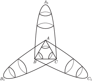
Refer to caption
Figure 8. Complex ℳ=Ξ/IMG(f)\mathcal{M}=\Xi/\mathop{\mathrm{IMG}}(f)

The covering pn:ℳn+1→ℳnp_{n}:\mathcal{M}_{n+1}\rightarrow\mathcal{M}_{n} is induced by the correspondence (ξ⊗x)↦ξ(\xi\otimes x)\mapsto\xi, where ξ∈Ξn=Ξ⊗𝔐f⊗n\xi\in\Xi_{n}=\Xi\otimes\mathfrak{M}_{f}^{\otimes n} and x∈𝔐fx\in\mathfrak{M}_{f}.

We will denote by [ξ][\xi] the image of ξ∈Ξn\xi\in\Xi_{n} in ℳn\mathcal{M}_{n}, i.e., the IMG(f)\mathop{\mathrm{IMG}}(f)-orbit of ξ\xi.

Proposition 5.9.

The covering pn:ℳn+1→ℳnp_{n}:\mathcal{M}_{n+1}\rightarrow\mathcal{M}_{n} acts by the rule

pn​([ξ⊗1])\displaystyle p_{n}([\xi\otimes\mathit{1}]) =[ξ],\displaystyle=[\xi], pn​([ξ⊗2])\displaystyle\quad p_{n}([\xi\otimes\mathit{2}]) =[ξ],\displaystyle=[\xi],
pn​([ξ⊗3])\displaystyle p_{n}([\xi\otimes\mathit{3}]) =[ξ⋅a],\displaystyle=[\xi\cdot a], pn​([ξ⊗4])\displaystyle\quad p_{n}([\xi\otimes\mathit{4}]) =[ξ⋅a],\displaystyle=[\xi\cdot a],

and

pn​([ξ⊗1⋅a])\displaystyle p_{n}([\xi\otimes\mathit{1}\cdot a]) =[ξ⋅a],\displaystyle=[\xi\cdot a], pn​([ξ⊗2⋅a])\displaystyle\quad p_{n}([\xi\otimes\mathit{2}\cdot a]) =[ξ⋅a],\displaystyle=[\xi\cdot a],
pn​([ξ⊗3])\displaystyle p_{n}([\xi\otimes\mathit{3}]) =[ξ],\displaystyle=[\xi], pn​([ξ⊗4])\displaystyle\quad p_{n}([\xi\otimes\mathit{4}]) =[ξ].\displaystyle=[\xi].
Proof.

We have for ξ∈Ξn\xi\in\Xi_{n}:

ξ⊗3=ξ⋅c⊗3⋅b,\xi\otimes\mathit{3}=\xi\cdot c\otimes\mathit{3}\cdot b,

hence pn​([ξ⊗3])=[ξ⋅c]=[ξ⋅a]p_{n}([\xi\otimes\mathit{3}])=[\xi\cdot c]=[\xi\cdot a]. Similarly,

ξ⊗4=ξ⋅c⊗4⋅b,\xi\otimes\mathit{4}=\xi\cdot c\otimes\mathit{4}\cdot b,

implies that pn​([ξ⊗4])=[ξ⋅a]p_{n}([\xi\otimes\mathit{4}])=[\xi\cdot a].

Since

ξ⊗1⋅a=ξ⋅b​β⊗1,\xi\otimes\mathit{1}\cdot a=\xi\cdot b\beta\otimes\mathit{1},

pn​([ξ⊗1⋅a])=[ξ⋅b​β]=[ξ⋅a]p_{n}([\xi\otimes\mathit{1}\cdot a])=[\xi\cdot b\beta]=[\xi\cdot a]. Similarly, since

ξ⊗2⋅a=ξ⋅b​α​β​α⊗2,\xi\otimes\mathit{2}\cdot a=\xi\cdot b\alpha\beta\alpha\otimes\mathit{2},

pn​([ξ⊗2⋅a])=[ξ⋅b​α​β​α]=[ξ⋅a]p_{n}([\xi\otimes\mathit{2}\cdot a])=[\xi\cdot b\alpha\beta\alpha]=[\xi\cdot a].

Equalities

ξ⊗3⋅a=ξ⊗3⋅b⋅b​a,ξ⊗4⋅a=ξ⊗4⋅b⋅b​a\xi\otimes\mathit{3}\cdot a=\xi\otimes\mathit{3}\cdot b\cdot ba,\quad\xi\otimes\mathit{4}\cdot a=\xi\otimes\mathit{4}\cdot b\cdot ba

show that pn​([ξ⊗i⋅a])=[ξ]p_{n}([\xi\otimes i\cdot a])=[\xi] for i∈{3,4}i\in\{\mathit{3},\mathit{4}\}. ∎

Equivariance of In:Ξn+1→ΞnI_{n}:\Xi_{n+1}\rightarrow\Xi_{n} and the fact that In​(𝒯n+1)=𝒯nI_{n}(\mathcal{T}_{n+1})=\mathcal{T}_{n} imply that for any ξ∈𝒯n+1\xi\in\mathcal{T}_{n+1}

ιn​([ξ])=[In​(ξ)],ιn​([ξ⋅a])=[In​(ξ)⋅a].\iota_{n}([\xi])=[I_{n}(\xi)],\qquad\iota_{n}([\xi\cdot a])=[I_{n}(\xi)\cdot a].

5.8. Spaces ℳn\mathcal{M}_{n} as subsets of the Julia set

Restriction of the map I:𝒯1→𝒯0I:\mathcal{T}_{1}\rightarrow\mathcal{T}_{0} onto closure of 𝒯1∖(C1​A​B​C⊗{2,3})\mathcal{T}_{1}\setminus(C_{1}ABC\otimes\{\mathit{2},\mathit{3}\}) is a homeomorphism (see Figures 6, 7 and definition of II in Subsection 5.6). Let Θ:𝒯0→𝒯1\Theta:\mathcal{T}_{0}\rightarrow\mathcal{T}_{1} be its inverse.

It is checked directly that for every g∈𝔄g\in\mathfrak{A} we have Θ⁡(Kg,0)⊆Kg,1\Theta(K_{g,0})\subseteq K_{g,1}. Suppose that ξ⋅g1=ξ⋅g2\xi\cdot g_{1}=\xi\cdot g_{2} for g1,g2∈Γg_{1},g_{2}\in\Gamma and ξ∈𝒯0\xi\in\mathcal{T}_{0}. Then ξ=ξ⋅g2​g1−1\xi=\xi\cdot g_{2}g_{1}^{-1}, hence g2​g1−1g_{2}g_{1}^{-1} belongs to the stabilizer Γξ\Gamma_{\xi} of ξ\xi. The stabilizer of Θ⁡(ξ)\Theta(\xi) contains Γξ\Gamma_{\xi}, by Lemma 5.3, since Θ⁡(Kg,0)⊆Kg,1\Theta(K_{g,0})\subseteq K_{g,1} and all transformations κg,1\kappa_{g,1} act trivially. Consequently, Θ⁡(ξ)⋅g1=Θ⁡(ξ)⋅g2\Theta(\xi)\cdot g_{1}=\Theta(\xi)\cdot g_{2}.

We have proved that Θ\Theta can be extended by the rule Θ⁡(ξ⋅g)=Θ⁡(ξ)⋅g\Theta(\xi\cdot g)=\Theta(\xi)\cdot g to a Γ\Gamma-equivariant map Θ:Ξ→Ξ⊗𝔐\Theta:\Xi\rightarrow\Xi\otimes\mathfrak{M}. It will be a section of the map I:Ξ⊗𝔐→ΞI:\Xi\otimes\mathfrak{M}\rightarrow\Xi, i.e., I∘Θ:Ξ→ΞI\circ\Theta:\Xi\rightarrow\Xi is identical.

Define

Θn​(ξ⊗v)=Θ⁡(ξ)⊗v\Theta_{n}(\xi\otimes v)=\Theta(\xi)\otimes v

for ξ∈Ξ\xi\in\Xi and v∈𝔐⊗nv\in\mathfrak{M}^{\otimes n}. The map Θn\Theta_{n} is well defined by equivariance of Θ\Theta. We get hence a sequence Θn:Ξn→Ξn+1\Theta_{n}:\Xi_{n}\rightarrow\Xi_{n+1} of sections of the maps In:Ξn+1→ΞnI_{n}:\Xi_{n+1}\rightarrow\Xi_{n}.

Denote by θn:ℳn→ℳn+1\theta_{n}:\mathcal{M}_{n}\rightarrow\mathcal{M}_{n+1} the maps induced by Θn\Theta_{n} on the orbispaces ℳn=Ξn/IMG(f)\mathcal{M}_{n}=\Xi_{n}/\mathop{\mathrm{IMG}}(f). The maps θn\theta_{n} are sections of the maps ιn:ℳn+1→ℳn\iota_{n}:\mathcal{M}_{n+1}\rightarrow\mathcal{M}_{n}.

We get hence natural homeomorphism θ~n\widetilde{\theta}_{n} of the space ℳn\mathcal{M}_{n} with a subset of the inverse limit ℳ∞≈𝒥IMG(f)\mathcal{M}_{\infty}\approx\mathcal{J}_{\mathop{\mathrm{IMG}}(f)}. It is the limit of the maps θn+k∘θn+k−1∘⋯∘θn:ℳn→ℳn+k+1\theta_{n+k}\circ\theta_{n+k-1}\circ\cdots\circ\theta_{n}:\mathcal{M}_{n}\rightarrow\mathcal{M}_{n+k+1} as k→∞k\to\infty.

The next theorem is now straightforward.

Theorem 5.10.

Let θ~n:ℳn→ℳ∞\widetilde{\theta}_{n}:\mathcal{M}_{n}\rightarrow\mathcal{M}_{\infty} be the limit of the maps θn+k∘⋯∘θn\theta_{n+k}\circ\cdots\circ\theta_{n}. Then

θ~n+1​(ℳn+1)⊃θ~n​(ℳn),p∞−1​(θ~n​(ℳn))=θ~n+1​(ℳn+1),pn=θ~n−1∘p∞∘θ~n+1,\widetilde{\theta}_{n+1}(\mathcal{M}_{n+1})\supset\widetilde{\theta}_{n}(\mathcal{M}_{n}),\quad p_{\infty}^{-1}(\widetilde{\theta}_{n}(\mathcal{M}_{n}))=\widetilde{\theta}_{n+1}(\mathcal{M}_{n+1}),\quad p_{n}={\widetilde{\theta}}^{-1}_{n}\circ p_{\infty}\circ\widetilde{\theta}_{n+1},

and the set ⋃n≥1θ~n​(ℳn)\bigcup_{n\geq 1}\widetilde{\theta}_{n}(\mathcal{M}_{n}) is dense in ℳ∞\mathcal{M}_{\infty}.

We will give later a natural description of the sets θ~n​(ℳn)\widetilde{\theta}_{n}(\mathcal{M}_{n}) as subsets of the Julia set of ff.

6. Skew product decomposition

6.1. The projection (z,w)↦w(z,w)\mapsto w

Projection (z,w)↦w(z,w)\mapsto w is a semicojugacy of ff with the rational function f^=(1−2/w)2\widehat{f}=(1-2/w)^{2}. By functoriality of the iterated monodromy groups (see [Nek08b]), the projection induces a group homomorphism

ν:IMG(f)→IMG(f^)\nu:\mathop{\mathrm{IMG}}(f)\rightarrow\mathop{\mathrm{IMG}}(\widehat{f})

and a morphism

μ:𝔐f→𝔐f^\mu:\mathfrak{M}_{f}\rightarrow\mathfrak{M}_{\widehat{f}}

of the corresponding self-similarity bimodules such that

μ⁡(g1⋅x⋅g2)=ν⁡(g1)⋅μ⁡(x)⋅ν⁡(g2)\mu(g_{1}\cdot x\cdot g_{2})=\nu(g_{1})\cdot\mu(x)\cdot\nu(g_{2})

for all g1,g2∈IMG(f)g_{1},g_{2}\in\mathop{\mathrm{IMG}}(f) and x∈𝔐fx\in\mathfrak{M}_{f}. The images of the generators α,β,γ\alpha,\beta,\gamma in IMG(f^)\mathop{\mathrm{IMG}}(\widehat{f}) are trivial (since they correspond to loops in which ww is constant). The images of the generators ss and tt are generators of IMG(f^)\mathop{\mathrm{IMG}}(\widehat{f}) (which we will also denote ss and tt) corresponding to the loops around the post-critical points 00 and 11 of f^\widehat{f}, respectively (see Figure 2). The basis elements 1,2∈𝖷\mathit{1},\mathit{2}\in\mathsf{X} will be mapped by μ\mu to the same element of 𝔐f^\mathfrak{M}_{\widehat{f}}, since the corresponding coset representatives ε,α\varepsilon,\alpha are mapped to the same element ε\varepsilon of IMG(f^)\mathop{\mathrm{IMG}}(\widehat{f}). Similarly the elements 3⋅b,4⋅b∈𝔐f\mathit{3}\cdot b,\mathit{4}\cdot b\in\mathfrak{M}_{f} corresponding to the last two coordinates of the wreath recursion from Theorem 4.3 will be mapped to the same element by μ\mu.

Consequently, applying the maps ν\nu and μ\mu to the wreath recursion of Theorem 4.3, we get the following wreath recursion generating IMG(f^)\mathop{\mathrm{IMG}}(\widehat{f})

(10) t=(t−1​s−1,t),s=σ,t=(t^{-1}s^{-1},t),\qquad s=\sigma,

where σ\sigma is the transposition. If {𝟏′,𝟐′}\{\mathbf{1}^{\prime},\mathbf{2}^{\prime}\} is the basis of the bimodule 𝔐f^\mathfrak{M}_{\widehat{f}} corresponding to this wreath recursion, then

μ⁡(1)=μ⁡(2)=𝟏′,μ⁡(3⋅b)=μ⁡(4⋅b)=𝟐′.\mu(\mathit{1})=\mu(\mathit{2})=\mathbf{1}^{\prime},\qquad\mu(\mathit{3}\cdot b)=\mu(\mathit{4}\cdot b)=\mathbf{2}^{\prime}.

Let Γ^{\widehat{\Gamma}} be the group generated by

a=σ,b=(a,c),c=(b,b).a=\sigma,\quad b=(a,c),\quad c=(b,b).

It is a quotient of the group Γ\Gamma as a self-similar group. The corresponding epimorphisms of groups and self-similarity bimodules (which we will also denote by μ:𝔐→𝔐Γ^\mu:\mathfrak{M}\rightarrow\mathfrak{M}_{\widehat{\Gamma}} and ν:Γ→Γ^\nu:\Gamma\rightarrow{\widehat{\Gamma}}, as they are extensions of the maps μ\mu and ν\nu) are defined by

μ⁡(1)=μ⁡(2)=𝟏,μ⁡(3)=μ⁡(4)=𝟐,\mu(\mathit{1})=\mu(\mathit{2})=\mathbf{1},\qquad\mu(\mathit{3})=\mu(\mathit{4})=\mathbf{2},

and by ν⁡(α)=ε\nu(\alpha)=\varepsilon, ν⁡(β)=ε\nu(\beta)=\varepsilon, ν⁡(γ)=ε\nu(\gamma)=\varepsilon, ν⁡(a)=a\nu(a)=a, ν⁡(b)=b\nu(b)=b, ν⁡(c)=c\nu(c)=c, where 𝟏′=𝟏\mathbf{1}^{\prime}=\mathbf{1} and 𝟐′=𝟐⋅b\mathbf{2}^{\prime}=\mathbf{2}\cdot b.

It is proved in [Nek07] that the group Γ^{\widehat{\Gamma}} is given by the presentation

Γ^≅⟨a,b,c|a2=b2=c2=(ac)2=(ab)4=(bc)4=ε⟩,{\widehat{\Gamma}}\cong\langle a,b,c\;|\;a^{2}=b^{2}=c^{2}=(ac)^{2}=(ab)^{4}=(bc)^{4}=\varepsilon\rangle,

and hence is isomorphic to the group generated by reflections of the Euclidean space with respect to the sides of an isosceles rectangular triangle (so that bb is the reflection with respect to the hypothenuse).

Let us take, for instance, triangle 𝒟⊂ℝ2\mathcal{D}\subset\mathbb{R}^{2} with the vertices A′=(1,0)A^{\prime}=(1,0), B′=(0,0)B^{\prime}=(0,0), and C′=(1,1)C^{\prime}=(1,1). Let the generators aa, bb, and cc correspond to reflections with respect to the lines B′​C′B^{\prime}C^{\prime}, A′​C′A^{\prime}C^{\prime}, and B′​A′B^{\prime}A^{\prime}, respectively, as it is shown on Figure 9.

Refer to caption
Figure 9. Triangle 𝒟\mathcal{D}

It follows from Proposition 5.1 (and it is also easy to prove directly, see [Nek07]) that the nucleus of Γ^{\widehat{\Gamma}} is the union of the groups

Γ^A\displaystyle{\widehat{\Gamma}}_{A} =\displaystyle= ⟨b,c⟩=ν⁡(ΓA)=ν⁡(ΓA1)≅D4,\displaystyle\langle b,c\rangle=\nu(\Gamma_{A})=\nu(\Gamma_{A_{1}})\cong D_{4},
Γ^B\displaystyle{\widehat{\Gamma}}_{B} =\displaystyle= ⟨a,c⟩=ν⁡(ΓB)=ν⁡(ΓB1)≅D2,\displaystyle\langle a,c\rangle=\nu(\Gamma_{B})=\nu(\Gamma_{B_{1}})\cong D_{2},
Γ^C\displaystyle{\widehat{\Gamma}}_{C} =\displaystyle= ⟨a,b⟩=ν⁡(ΓC)=ν⁡(ΓC1)≅D4.\displaystyle\langle a,b\rangle=\nu(\Gamma_{C})=\nu(\Gamma_{C_{1}})\cong D_{4}.

The pairwise intersections of the subgroups of the nucleus are the obvious ones:

Γ^C​B=⟨a,b⟩∩⟨a,c⟩=⟨a⟩,Γ^C​A=⟨a,b⟩∩⟨b,c⟩=⟨b⟩,Γ^A​B=⟨b,c⟩∩⟨a,c⟩=⟨c⟩,{\widehat{\Gamma}}_{CB}=\langle a,b\rangle\cap\langle a,c\rangle=\langle a\rangle,\quad{\widehat{\Gamma}}_{CA}=\langle a,b\rangle\cap\langle b,c\rangle=\langle b\rangle,\quad{\widehat{\Gamma}}_{AB}=\langle b,c\rangle\cap\langle a,c\rangle=\langle c\rangle,

and are groups of order two. Denote

𝒢^={Γ^A,Γ^B,Γ^C,Γ^B​C,Γ^C​A,Γ^A​B,{ε}},\widehat{\mathcal{G}}=\left\{{\widehat{\Gamma}}_{A},{\widehat{\Gamma}}_{B},{\widehat{\Gamma}}_{C},{\widehat{\Gamma}}_{BC},{\widehat{\Gamma}}_{CA},{\widehat{\Gamma}}_{AB},\{\varepsilon\}\right\},

and let Ξ^{\widehat{\Xi}} be the image of the complex Ξ\Xi under the map ν:Γ→Γ^\nu:\Gamma\rightarrow{\widehat{\Gamma}}, i.e., the complex associated with the poset of sets of the form G⋅hG\cdot h for h∈Γ^h\in{\widehat{\Gamma}} and G∈𝒢^G\in\widehat{\mathcal{G}}. The complex Ξ^{\widehat{\Xi}} is isomorphic to the barycentric subdivision of the simplicial complex obtained by tiling the Euclidean plane by the images of the triangle 𝒟\mathcal{D} under the action of the group Γ^{\widehat{\Gamma}}. The groups Γ^A,Γ^B,Γ^C{\widehat{\Gamma}}_{A},{\widehat{\Gamma}}_{B},{\widehat{\Gamma}}_{C} correspond to the vertices A′A^{\prime}, B′B^{\prime}, C′C^{\prime} of the triangle 𝒟\mathcal{D}, respectively. The groups Γ^A​B,Γ^B​C,Γ^A​C{\widehat{\Gamma}}_{AB},{\widehat{\Gamma}}_{BC},{\widehat{\Gamma}}_{AC} correspond to the edges A′​B′A^{\prime}B^{\prime}, B′​C′B^{\prime}C^{\prime}, A′​C′A^{\prime}C^{\prime}, respectively. Each group is the stabilizer of the corresponding simplex of Ξ^{\widehat{\Xi}}. The triangle 𝒟\mathcal{D} is a fundamental domain of the action of Γ^{\widehat{\Gamma}} on Ξ^{\widehat{\Xi}}.

Define the map P:𝒯0→𝒟P:\mathcal{T}_{0}\rightarrow\mathcal{D} so that it is affine on the tetrahedra A1​A​B​CA_{1}ABC, B1​A​B​CB_{1}ABC, C1​A​B​CC_{1}ABC and acts on their vertices by the rules

(11) P⁡(A)\displaystyle P(A) =A′,\displaystyle=A^{\prime}, P⁡(B)\displaystyle\quad P(B) =B′,\displaystyle=B^{\prime}, P⁡(C)\displaystyle\quad P(C) =C′,\displaystyle=C^{\prime},
(12) P⁡(A1)\displaystyle P(A_{1}) =A′,\displaystyle=A^{\prime}, P⁡(B1)\displaystyle\quad P(B_{1}) =B′,\displaystyle=B^{\prime}, P⁡(C1)\displaystyle\quad P(C_{1}) =C′,\displaystyle=C^{\prime},

i.e., mapping a vertex corresponding to ΓX∈𝒢\Gamma_{X}\in\mathcal{G} to the vertex corresponding to its image under ν\nu. Recall that we have introduced in Subsection 5.6 a Euclidean structure on 𝒯0\mathcal{T}_{0} identifying it with a subset of ℝ5\mathbb{R}^{5}. The points A,B,CA,B,C become vertices of an isosceles right triangle after this identification. The vectors A​A1→\overrightarrow{AA_{1}}, B​B1→\overrightarrow{BB_{1}}, and C​C1→\overrightarrow{CC_{1}} are orthogonal to the triangle A​B​CABC. Consequently, if we identify A′,B′,C′A^{\prime},B^{\prime},C^{\prime} with the points points A,B,CA,B,C of ℝ5\mathbb{R}^{5}, then PP will be the orthogonal projection of 𝒯0\mathcal{T}_{0} onto the plain spanned by B​A→\vec{BA} and B​C→\vec{BC}.

The map P:𝒯0→𝒟P:\mathcal{T}_{0}\rightarrow\mathcal{D} can be extended to a continuous map P:Ξ→Ξ^P:\Xi\rightarrow{\widehat{\Xi}} such that

(13) P⁡(ξ⋅g)=P⁡(ξ)⋅ν⁡(g)P(\xi\cdot g)=P(\xi)\cdot\nu(g)

for every ξ∈Ξ\xi\in\Xi and g∈Γg\in\Gamma. The map PP will map the vertex corresponding to a coset ΓX⋅g\Gamma_{X}\cdot g to the vertex corresponding to the coset ν⁡(ΓX⋅g)\nu(\Gamma_{X}\cdot g).

Denote by L:Ξ^⊗𝔐Γ^→Ξ^L:{\widehat{\Xi}}\otimes\mathfrak{M}_{\widehat{\Gamma}}\rightarrow{\widehat{\Xi}} the Γ^{\widehat{\Gamma}}-equivariant map induced by I:Ξ⊗𝔐→ΞI:\Xi\otimes\mathfrak{M}\rightarrow\Xi, where 𝔐Γ^\mathfrak{M}_{\widehat{\Gamma}} is the self-similarity Γ^{\widehat{\Gamma}}-bimodule. It is given by

L⁡(P⁡(ξ⊗v))=P⁡(I⁡(ξ⊗v)),L(P(\xi\otimes v))=P(I(\xi\otimes v)),

and is well defined by equivariance of II and property (13).

Formulae defining II imply that

L⁡(A′⊗𝟏)\displaystyle L(A^{\prime}\otimes\mathbf{1}) =C′,\displaystyle=C^{\prime}, L⁡(B′⊗𝟏)\displaystyle\quad L(B^{\prime}\otimes\mathbf{1}) =(A′​C′),\displaystyle=(A^{\prime}C^{\prime}), L⁡(C′⊗𝟏)\displaystyle\quad L(C^{\prime}\otimes\mathbf{1}) =B′,\displaystyle=B^{\prime},
L⁡(A′⊗𝟐)\displaystyle L(A^{\prime}\otimes\mathbf{2}) =A′,\displaystyle=A^{\prime}, L⁡(B′⊗𝟐)\displaystyle\quad L(B^{\prime}\otimes\mathbf{2}) =(A′​C′),\displaystyle=(A^{\prime}C^{\prime}), L⁡(C′⊗𝟐)\displaystyle\quad L(C^{\prime}\otimes\mathbf{2}) =B′.\displaystyle=B^{\prime}.

One checks directly using equivariance of the map LL (see also [Nek08b, 4.8.3]) that the maps ξ↦L⁡(ξ⊗x)\xi\mapsto L(\xi\otimes x) act on Ξ^≈ℝ2\widehat{\Xi}\approx\mathbb{R}^{2} by affine transformations with the linear parts (−1/2−1/21/2−1/2)\left(\begin{array}[]{rr}-1/2&-1/2\\ 1/2&-1/2\end{array}\right) and (1/2−1/2−1/2−1/2)\left(\begin{array}[]{cc}1/2&-1/2\\ -1/2&-1/2\end{array}\right) for x=𝟏x=\mathbf{1} and x=𝟐x=\mathbf{2}, respectively. Compare these matrices with the top left corners of the matrices ℐx\mathcal{I}_{x} in the proof of Proposition 5.5. Note that in both cases the transformation L(⋅⊗x)L(\cdot\otimes x) divides all distances of ℝ2\mathbb{R}^{2} by 2\sqrt{2}.

It is proved in [Nek08b] that the map L:Ξ^⊗𝔐Γ^→Ξ^L:{\widehat{\Xi}}\otimes\mathfrak{M}_{\widehat{\Gamma}}\rightarrow{\widehat{\Xi}} and hence the maps Ln:Ξ^⊗𝔐Γ^⊗(n+1)→Ξ^⊗𝔐Γ^⊗nL_{n}:{\widehat{\Xi}}\otimes\mathfrak{M}_{\widehat{\Gamma}}^{\otimes(n+1)}\rightarrow{\widehat{\Xi}}\otimes\mathfrak{M}_{\widehat{\Gamma}}^{\otimes n} are homeomorphisms.

By equivariance of the maps LnL_{n}, the action of Γ^{\widehat{\Gamma}} on Ξ^⊗𝔐⊗n{\widehat{\Xi}}\otimes\mathfrak{M}^{\otimes n} is obtained by conjugating the action of Γ^{\widehat{\Gamma}} on Ξ^{\widehat{\Xi}} by the homeomorphism LnL_{n}. One can show that the fundamental domains 𝒟n=𝒟⊗{𝟏,𝟐}n\mathcal{D}_{n}=\mathcal{D}\otimes\{\mathbf{1},\mathbf{2}\}^{n} are rectangular isosceles triangles of area 2n−12^{n-1} tiled by isometric copies of the triangle 𝒟\mathcal{D}, as it is shown on Figure 10. The orbispaces Ξ^⊗𝔐⊗n/Γ^{\widehat{\Xi}}\otimes\mathfrak{M}^{\otimes n}/{\widehat{\Gamma}} can be identified with the fundamental domains 𝒟n\mathcal{D}_{n} (i.e., the natural map from 𝒟n\mathcal{D}_{n} to the orbispace is a homeomorphism).

Refer to caption
Figure 10. The sets 𝒟n\mathcal{D}_{n}

The spaces 𝒮n=Ξ^⊗𝔐⊗n/IMG(f^)\mathcal{S}_{n}={\widehat{\Xi}}\otimes\mathfrak{M}^{\otimes n}/\mathop{\mathrm{IMG}}(\widehat{f}) are obtained by “doubling” the triangles: by taking two copies 𝒟n\mathcal{D}_{n} and 𝒟n⋅a\mathcal{D}_{n}\cdot a, and pasting them together along the boundary.

Denote by

qn:𝒮n+1→𝒮n,λn:𝒮n+1→𝒮nq_{n}:\mathcal{S}_{n+1}\rightarrow\mathcal{S}_{n},\quad\lambda_{n}:\mathcal{S}_{n+1}\rightarrow\mathcal{S}_{n}

the covering induced by the projection ζ⊗v​x↦ζ⊗v\zeta\otimes vx\mapsto\zeta\otimes v and the map induced by LnL_{n}. We will also denote 𝒮=𝒮0\mathcal{S}=\mathcal{S}_{0}, q=q0q=q_{0}, and λ=λ0\lambda=\lambda_{0}. The maps λn\lambda_{n} act on each copy of 𝒟n+1\mathcal{D}_{n+1} in 𝒮n+1\mathcal{S}_{n+1} as similitudes with coefficient 2/2\sqrt{2}/2. The covering qnq_{n} maps halves of each copy of 𝒟n+1\mathcal{D}_{n+1} isometrically to copies of 𝒟n\mathcal{D}_{n} in 𝒮n\mathcal{S}_{n} (according to the rules similar to the rules of Proposition 5.9).

We can identify the spaces Ξ^⊗𝔐Γ^⊗n{\widehat{\Xi}}\otimes\mathfrak{M}_{\widehat{\Gamma}}^{\otimes n} with ℂ\mathbb{C} in such a way that the group Γ^{\widehat{\Gamma}} acts on them as the group of all isometries of the lattice ℤ⁡[i]\mathbb{Z}[i], and the map LnL_{n} is identical (see [Nek08b, 4.8.2–3] for details). The subgroup IMG(f^)\mathop{\mathrm{IMG}}(\widehat{f}) of Γ^{\widehat{\Gamma}} acts then on Ξ^⊗𝔐Γ^⊗n≈ℂ{\widehat{\Xi}}\otimes\mathfrak{M}_{\widehat{\Gamma}}^{\otimes n}\approx\mathbb{C} as the group of affine transformations of the form z↦ik​z+z0z\mapsto i^{k}z+z_{0}, where k∈ℤk\in\mathbb{Z} and z0∈ℤ⁡[i]z_{0}\in\mathbb{Z}[i]. The coverings qn:𝒮n+1→𝒮nq_{n}:\mathcal{S}_{n+1}\rightarrow\mathcal{S}_{n} are induced then by the map z↦(1−i)​zz\mapsto(1-i)z.

It follows that the limit dynamical system of IMG(f^)\mathop{\mathrm{IMG}}(\widehat{f}) is conjugate with the map Fi−1:𝒮0→𝒮0F_{i-1}:\mathcal{S}_{0}\rightarrow\mathcal{S}_{0} induced by the transformation z↦(1−i)​zz\mapsto(1-i)z of ℂ\mathbb{C}. It is well known (and follows from the general theory of iterated monodromy groups) that the map F1−iF_{1-i} is conjugate to the rational function f^\widehat{f}. The conjugating map is induced on 𝒮0\mathcal{S}_{0} by the map z↦(℘⁡(z))2z\mapsto\left(\wp(z)\right)^{2}, where ℘\wp is the Weierstrass function associated with the lattice ℤ⁡[i]\mathbb{Z}[i].

6.2. Fibers of ℳn→𝒮n\mathcal{M}_{n}\rightarrow\mathcal{S}_{n}

Denote by Pn:Ξ⊗𝔐⊗n→Ξ^⊗𝔐Γ^⊗nP_{n}:\Xi\otimes\mathfrak{M}^{\otimes n}\rightarrow{\widehat{\Xi}}\otimes\mathfrak{M}_{\widehat{\Gamma}}^{\otimes n} the map given by

Pn​(ξ⊗v)=P⁡(ξ)⊗μ⁡(v),P_{n}(\xi\otimes v)=P(\xi)\otimes\mu(v),

where ξ∈Ξ\xi\in\Xi and v∈𝔐⊗nv\in\mathfrak{M}^{\otimes n}. We also denote P0=PP_{0}=P.

The next proposition follows directly from the definitions.

Proposition 6.1.

The map Pn:Ξ⊗𝔐⊗(n+1)→Ξ^⊗𝔐Γ^⊗nP_{n}:\Xi\otimes\mathfrak{M}^{\otimes(n+1)}\rightarrow{\widehat{\Xi}}\otimes\mathfrak{M}_{\widehat{\Gamma}}^{\otimes n} induces maps ρn:ℳn→𝒮n\rho_{n}:\mathcal{M}_{n}\rightarrow\mathcal{S}_{n} making the diagrams

ℳn+1→pnℳn↓ρn+1↓ρn𝒮n+1→qn𝒮n,ℳn+1→ιnℳn↓ρn+1↓ρn𝒮n+1→λn𝒮n\begin{array}[]{ccc}\mathcal{M}_{n+1}&\stackrel{{\scriptstyle p_{n}}}{{\rightarrow}}&\mathcal{M}_{n}\\ \Big\downarrow\hbox to0.0pt{$\vbox{\hbox{$\scriptstyle\rho_{n+1}$}}$\hss}&&\Big\downarrow\hbox to0.0pt{$\vbox{\hbox{$\scriptstyle\rho_{n}$}}$\hss}\\ \mathcal{S}_{n+1}&\stackrel{{\scriptstyle q_{n}}}{{\rightarrow}}&\mathcal{S}_{n}\end{array},\qquad\begin{array}[]{ccc}\mathcal{M}_{n+1}&\stackrel{{\scriptstyle\iota_{n}}}{{\rightarrow}}&\mathcal{M}_{n}\\ \Big\downarrow\hbox to0.0pt{$\vbox{\hbox{$\scriptstyle\rho_{n+1}$}}$\hss}&&\Big\downarrow\hbox to0.0pt{$\vbox{\hbox{$\scriptstyle\rho_{n}$}}$\hss}\\ \mathcal{S}_{n+1}&\stackrel{{\scriptstyle\lambda_{n}}}{{\rightarrow}}&\mathcal{S}_{n}\end{array}

commutative.

Denote by Zα,n,Zβ,n,Zγ,nZ_{\alpha,n},Z_{\beta,n},Z_{\gamma,n} the sets of points of ℳn\mathcal{M}_{n} of the form [ξ][\xi] and [ξ⋅a][\xi\cdot a], where ξ∈𝒯n\xi\in\mathcal{T}_{n} is a fixed point of the transformation κα,n\kappa_{\alpha,n}, κβ,n\kappa_{\beta,n}, κγ,n\kappa_{\gamma,n}, respectively.

Theorem 6.2.

The set ρn−1​(ξ)\rho_{n}^{-1}(\xi) is a finite tree for every ξ∈𝒮n\xi\in\mathcal{S}_{n}.

The map pn:ℳn+1→ℳnp_{n}:\mathcal{M}_{n+1}\rightarrow\mathcal{M}_{n} restricts for every ξ∈ℳn+1\xi\in\mathcal{M}_{n+1} to a degree two branched covering ρn+1−1​(ξ)→ρn−1​(qn​(ξ))\rho_{n+1}^{-1}(\xi)\rightarrow\rho_{n}^{-1}(q_{n}(\xi)). Denote by Zn+1​(ξ)Z_{n+1}(\xi) its critical point.

Intersections of Zα,nZ_{\alpha,n}, Zβ,nZ_{\beta,n}, and Zγ,nZ_{\gamma,n} with ρn−1​(ξ)\rho_{n}^{-1}(\xi) are singletons. Let us denote them by Zα,n​(ξ)Z_{\alpha,n}(\xi), Zβ,n​(ξ)Z_{\beta,n}(\xi), and Zγ,n​(ξ)Z_{\gamma,n}(\xi), respectively.

Let ξ=[ζ⊗x]∈𝒮n+1\xi=[\zeta\otimes x]\in\mathcal{S}_{n+1}, where ζ∈𝒟n\zeta\in\mathcal{D}_{n} and x∈{𝟏,𝟏⋅a,𝟐,𝟐⋅a}x\in\{\mathbf{1},\mathbf{1}\cdot a,\mathbf{2},\mathbf{2}\cdot a\}. The tree ρn+1−1​(ξ)\rho_{n+1}^{-1}(\xi) is union of two trees T1T_{1} and T2T_{2} such that

  • (i)

    the common point of T1T_{1} and T2T_{2} is Zn+1​(ξ)Z_{n+1}(\xi);

  • (ii)

    restrictions of the map pn:ρn+1−1​(ξ)→ρn−1​(qn​(ξ))p_{n}:\rho_{n+1}^{-1}(\xi)\rightarrow\rho_{n}^{-1}(q_{n}(\xi)) onto T1T_{1} and T2T_{2} are homeomorphisms;

  • (iii)

    pn​(Zn+1​(ξ))=Zα,n​(qn​(ξ))p_{n}(Z_{n+1}(\xi))=Z_{\alpha,n}(q_{n}(\xi));

  • (iv)

    pn−1​(Zβ,n​(qn​(ξ)))∩T1=Zα,n+1​(ξ)p_{n}^{-1}(Z_{\beta,n}(q_{n}(\xi)))\cap T_{1}=Z_{\alpha,n+1}(\xi), and pn−1​(Zβ,n​(qn​(ξ)))∩T2=Zγ,n+1​(ξ)p_{n}^{-1}(Z_{\beta,n}(q_{n}(\xi)))\cap T_{2}=Z_{\gamma,n+1}(\xi);

  • (v)

    if x∈{𝟏,𝟏⋅a}x\in\{\mathbf{1},\mathbf{1}\cdot a\}, then pn−1​(Zγ,n​(qn​(ξ)))∩T1=Zβ,n+1​(ξ)p_{n}^{-1}(Z_{\gamma,n}(q_{n}(\xi)))\cap T_{1}=Z_{\beta,n+1}(\xi);

  • (vi)

    if x∈{𝟐,𝟐⋅a}x\in\{\mathbf{2},\mathbf{2}\cdot a\}, then pn−1​(Zγ,n​(qn​(ξ)))∩T2=Zβ,n+1​(ξ)p_{n}^{-1}(Z_{\gamma,n}(q_{n}(\xi)))\cap T_{2}=Z_{\beta,n+1}(\xi).

Proof.

The set ρn+1−1​([ζ⊗x])\rho_{n+1}^{-1}([\zeta\otimes x]) is equal to the set of points of the form [ξ⊗y][\xi\otimes y], where ξ∈𝒯n\xi\in\mathcal{T}_{n} and y∈𝖷⋅{ε,a}y\in\mathsf{X}\cdot\{\varepsilon,a\} are such that Pn​(ξ)=ζP_{n}(\xi)=\zeta and μ⁡(y)=x\mu(y)=x. Note that for every x∈{𝟏,𝟐}x\in\{\mathbf{1},\mathbf{2}\} there exists exactly two elements y1,y2∈𝖷⋅{ε,a}y_{1},y_{2}\in\mathsf{X}\cdot\{\varepsilon,a\} such that μ⁡(y)=x\mu(y)=x.

Depending on xx, restriction of the map pn+1p_{n+1} onto ρn+1−1​([ζ⊗x])\rho_{n+1}^{-1}([\zeta\otimes x]) acts by the rule

[η⊗y]↦[η],or[η⊗y]↦[η⋅a],[\eta\otimes y]\mapsto[\eta],\quad\text{or}\quad[\eta\otimes y]\mapsto[\eta\cdot a],

as it is described in Proposition 5.9.

It follows that the restriction is two-to-one except for the points η\eta such that [η⊗y1]=[η⊗y2][\eta\otimes y_{1}]=[\eta\otimes y_{2}], where {y1,y2}=μ−1​(x)\{y_{1},y_{2}\}=\mu^{-1}(x). It is sufficient to consider the case x∈{𝟏,𝟐}x\in\{\mathbf{1},\mathbf{2}\} and y∈𝖷y\in\mathsf{X}. The equality [η⊗y1]=[η⊗y2][\eta\otimes y_{1}]=[\eta\otimes y_{2}] is equivalent to existence of an element g∈𝒩g\in\mathcal{N} such that η⋅g=η\eta\cdot g=\eta and g⋅y1=y2⋅hg\cdot y_{1}=y_{2}\cdot h for h∈IMG(f)h\in\mathop{\mathrm{IMG}}(f). Note that since μ⁡(y1)=μ⁡(y2)=x\mu(y_{1})=\mu(y_{2})=x, the element g∈𝒩g\in\mathcal{N} has an even number of factors aa in its decomposition into a product of generators. It follows now from h∈IMG(f)h\in\mathop{\mathrm{IMG}}(f) that gg has an even total number of factors bb and cc, i.e., that gg is an element of the set ⟨α,β,γ⟩⋅⟨b​c⟩\langle\alpha,\beta,\gamma\rangle\cdot\langle bc\rangle. Since y1≠y2y_{1}\neq y_{2}, the element gg contains an odd number of factors α\alpha. Looking through the groups ΓA,ΓB,ΓC,ΓA1,ΓB1,ΓC1\Gamma_{A},\Gamma_{B},\Gamma_{C},\Gamma_{A_{1}},\Gamma_{B_{1}},\Gamma_{C_{1}}, we conclude that

g∈⟨α,β⟩∪⟨α,γ⟩∪α⋅⟨b​c⟩.g\in\langle\alpha,\beta\rangle\cup\langle\alpha,\gamma\rangle\cup\alpha\cdot\langle bc\rangle.

Consequently, either g=αg=\alpha, or g∈𝒩∖𝔄g\in\mathcal{N}\setminus\mathfrak{A} and the stabilizer of the point η\eta contains α\alpha, by Lemma 5.3. In both cases η⋅α=η\eta\cdot\alpha=\eta, i.e., [η]∈Zα,n[\eta]\in Z_{\alpha,n}. In the other direction, if [η]∈Zα,n[\eta]\in Z_{\alpha,n}, then [η]=[η′][\eta]=[\eta^{\prime}] for η′⋅α=η′\eta^{\prime}\cdot\alpha=\eta^{\prime}, and then [η′⊗y1]=[η′⋅α⊗y1]=[η′⊗y2][\eta^{\prime}\otimes y_{1}]=[\eta^{\prime}\cdot\alpha\otimes y_{1}]=[\eta^{\prime}\otimes y_{2}].

We have shown that a point [η][\eta] has one preimage under the restriction of ρn+1\rho_{n+1} onto ρn+1−1​([ζ⊗x])\rho_{n+1}^{-1}([\zeta\otimes x]) if and only if [η]∈Zα,n[\eta]\in Z_{\alpha,n}. In all the other cases it has two preimages.

Let us prove by induction on nn that the intersections of Zα,nZ_{\alpha,n}, Zβ,nZ_{\beta,n}, and Zγ,nZ_{\gamma,n} with the fibers of the map ρn\rho_{n} are singletons.

It is true for n=0n=0. By Theorem 5.4, a point η⊗y∈𝒯n+1\eta\otimes y\in\mathcal{T}_{n+1}, for η∈𝒯n\eta\in\mathcal{T}_{n} and y∈𝖷y\in\mathsf{X}, belongs to Kα,n+1K_{\alpha,n+1} if and only if η∈Kβ,n\eta\in K_{\beta,n} and y∈{1,3}y\in\{\mathit{1},\mathit{3}\}.

We have

κα,n+1​(η⊗y)=κβ,n​(η)⊗y=η⋅β⊗y.\kappa_{\alpha,n+1}(\eta\otimes y)=\kappa_{\beta,n}(\eta)\otimes y=\eta\cdot\beta\otimes y.

If η⊗y=η⋅β⊗y\eta\otimes y=\eta\cdot\beta\otimes y, then it follows from Theorem 5.4 that η⋅β=η⋅g\eta\cdot\beta=\eta\cdot g and g⋅y=yg\cdot y=y for g∈⟨a,α,γ⟩g\in\langle a,\alpha,\gamma\rangle. But then η=η⋅β​g−1\eta=\eta\cdot\beta g^{-1}, which implies that β​g−1∈𝒩\beta g^{-1}\in\mathcal{N}, and then by Lemma 5.3 that η\eta is fixed under β\beta.

It follows now from the inductive assumption (since μ⁡(1)≠μ⁡(3)\mu(\mathit{1})\neq\mu(\mathit{3})) that intersection of Zα,n+1Z_{\alpha,n+1} with the fibers of ρn+1\rho_{n+1} are singletons.

Similarly, η⊗y\eta\otimes y belongs to Kγ,n+1K_{\gamma,n+1} if and only if η∈Kβ,n\eta\in K_{\beta,n} and y∈{2,4}y\in\{\mathit{2},\mathit{4}\}. By the same arguments as above, η⊗y\eta\otimes y is fixed under κγ,n+1\kappa_{\gamma,n+1} if and only if η\eta is fixed under κβ,n\kappa_{\beta,n}. Consequently, intersections of Zγ,n+1Z_{\gamma,n+1} with the fibers of ρn+1\rho_{n+1} are singletons.

A point η⊗y\eta\otimes y belongs to Kβ,n+1K_{\beta,n+1} if and only if η∈Kγ,n\eta\in K_{\gamma,n} and y∈{1,4}y\in\{\mathit{1},\mathit{4}\}, or η∈Ka​α​γ,n\eta\in K_{a\alpha\gamma,n} and y∈{1,4}y\in\{\mathit{1},\mathit{4}\}.

Suppose that η∈Kγ,n\eta\in K_{\gamma,n}. Then

κβ,n+1​(η⊗y)=η⋅γ⊗y.\kappa_{\beta,n+1}(\eta\otimes y)=\eta\cdot\gamma\otimes y.

Again, by Theorem 5.4, if η⊗y=η⋅γ⊗y\eta\otimes y=\eta\cdot\gamma\otimes y, then η⋅γ=η⋅g\eta\cdot\gamma=\eta\cdot g and g⋅y=yg\cdot y=y for some g∈⟨α,γ,a⟩g\in\langle\alpha,\gamma,a\rangle. The equality g⁡(y)=yg(y)=y implies that g∈{ε,γ,γα}g\in\{\varepsilon,\gamma,\gamma^{\alpha}\} (as γa=γα\gamma^{a}=\gamma^{\alpha} and ⟨a,α⟩\langle a,\alpha\rangle acts faithfully on 𝖷\mathsf{X}). The case g=γg=\gamma contradicts g⋅y=yg\cdot y=y and y∈{1,4}y\in\{\mathit{1},\mathit{4}\}. If g=γαg=\gamma^{\alpha}, then η\eta is fixed by γ​γα\gamma\gamma^{\alpha}, which implies by Lemma 5.3 that it is also fixed by γ\gamma. If g=εg=\varepsilon, then η⋅g=η⋅γ\eta\cdot g=\eta\cdot\gamma implies that η\eta is fixed by γ\gamma.

Suppose that η∈Ka​α​γ,n\eta\in K_{a\alpha\gamma,n} and y∈{1,4}y\in\{\mathit{1},\mathit{4}\}. Then κβ,n+1​(η⊗y)=η⋅a​α​γ⊗σ​π​(y)\kappa_{\beta,n+1}(\eta\otimes y)=\eta\cdot a\alpha\gamma\otimes\sigma\pi(y). If η⊗y=η⋅a​α​γ⊗σ​π​(y)\eta\otimes y=\eta\cdot a\alpha\gamma\otimes\sigma\pi(y), then there exists g∈⟨α,a,γ⟩g\in\langle\alpha,a,\gamma\rangle such that η⋅g=η⋅a​α​γ\eta\cdot g=\eta\cdot a\alpha\gamma and g⋅y=σ​π​(y)g\cdot y=\sigma\pi(y). The condition g⁡(y)=σ​π​(y)g(y)=\sigma\pi(y) implies that g∈{a​α,a​α​γ,a​α​γα}g\in\{a\alpha,a\alpha\gamma,a\alpha\gamma^{\alpha}\}. The condition g|y=εg|_{y}=\varepsilon eliminates the case g=a​α​γg=a\alpha\gamma. If g=a​αg=a\alpha, then η⋅g=η⋅a​α​γ\eta\cdot g=\eta\cdot a\alpha\gamma implies η⋅γ=ξ\eta\cdot\gamma=\xi (since a​αa\alpha commutes with γ\gamma). If g=a​α​γαg=a\alpha\gamma^{\alpha}, then η=η⋅γα\eta=\eta\cdot\gamma^{\alpha}, which also by Lemma 5.3 implies that η=η⋅γ\eta=\eta\cdot\gamma.

We see that in all cases [η]∈Zγ,n[\eta]\in Z_{\gamma,n}, hence intersections of Zβ,n+1Z_{\beta,n+1} with the fibers of ρn+1\rho_{n+1} are singletons.

Note that we have already proved that

pn​(Zα,n+1​(ξ))=pn​(Zγ,n+1​(ξ))=Zβ,n​(qn​(ξ))p_{n}(Z_{\alpha,n+1}(\xi))=p_{n}(Z_{\gamma,n+1}(\xi))=Z_{\beta,n}(q_{n}(\xi))

and pn​(Zβ,n+1​(ξ))=Zγ,n​(qn​(ξ))p_{n}(Z_{\beta,n+1}(\xi))=Z_{\gamma,n}(q_{n}(\xi)). The equality pn​(Zn+1​(ξ))=Zα,n​(qn​(ξ))p_{n}(Z_{n+1}(\xi))=Z_{\alpha,n}(q_{n}(\xi)) was also proved before.

By the proved above, the fiber ρn+1−1​(ζ⊗x)\rho_{n+1}^{-1}(\zeta\otimes x) is obtained by identifying in the sets ρn−1​(ζ)⊗y1\rho_{n}^{-1}(\zeta)\otimes y_{1} and ρn−1​(ζ)⊗y2\rho_{n}^{-1}(\zeta)\otimes y_{2} the points Zα,n​(ζ)⊗y1Z_{\alpha,n}(\zeta)\otimes y_{1} with Zα,n​(ζ)⊗y2Z_{\alpha,n}(\zeta)\otimes y_{2}. Since the fibers of ρ0\rho_{0} are trees, we get by induction that the fibers of ρn\rho_{n} are also trees. It also follows that the point Zn+1​(ζ⊗x)=Zα,n​(ζ)⊗y1=Zα,n​(ζ)⊗y2Z_{n+1}(\zeta\otimes x)=Z_{\alpha,n}(\zeta)\otimes y_{1}=Z_{\alpha,n}(\zeta)\otimes y_{2} separates the subtrees ρn−1​(ζ)⊗y1\rho_{n}^{-1}(\zeta)\otimes y_{1} and ρn−1​(ζ)⊗y2\rho_{n}^{-1}(\zeta)\otimes y_{2}. Let y1∈{1,1⋅a,3,3⋅a}y_{1}\in\{\mathit{1},\mathit{1}\cdot a,\mathit{3},\mathit{3}\cdot a\} and y2∈{2,2⋅a,4,4⋅a}y_{2}\in\{\mathit{2},\mathit{2}\cdot a,\mathit{4},\mathit{4}\cdot a\}. Then denote T1=ρn−1​(ζ)⊗y1T_{1}=\rho_{n}^{-1}(\zeta)\otimes y_{1} and T2=ρn−1​(ζ)⊗y2T_{2}=\rho_{n}^{-1}(\zeta)\otimes y_{2}.

The rest of the theorem follows now from the recurrent description of the sets Zα,nZ_{\alpha,n}, Zβ,nZ_{\beta,n}, and Zγ,nZ_{\gamma,n}, and the sets Kα,nK_{\alpha,n}, Kβ,nK_{\beta,n}, and Kγ,nK_{\gamma,n}. ∎

6.3. Unfolding trees and the map ιn\iota_{n}

Consider the embedding of the complex 𝒯0\mathcal{T}_{0} into ℝ5\mathbb{R}^{5} described in Subsection 5.6 and the embedding of 𝒟\mathcal{D} into ℝ2\mathbb{R}^{2} described in Subsection 6.1. Then projection P:𝒯0→𝒟P:\mathcal{T}_{0}\rightarrow\mathcal{D} acts as the map (x1,x2,x3,x4,x5)↦(x1,x2)(x_{1},x_{2},x_{3},x_{4},x_{5})\mapsto(x_{1},x_{2}). The fiber P−1​(x1,x2)P^{-1}(x_{1},x_{2}) is a union of three segments with one common end (x1,x2,0,0,0)(x_{1},x_{2},0,0,0). The other ends of the segments are Zα=Zα,0​((x1,x2))Z_{\alpha}=Z_{\alpha,0}((x_{1},x_{2})), Zβ=Zβ,0​((x1,x2))Z_{\beta}=Z_{\beta,0}((x_{1},x_{2})), Zγ=Zγ,0​((x1,x2))Z_{\gamma}=Z_{\gamma,0}((x_{1},x_{2})), respectively.

The point ZαZ_{\alpha} is the intersection of P−1​(x1,x2)P^{-1}(x_{1},x_{2}) with the plane A1​B​CA_{1}BC, hence it has coordinates (x1,x2,x1,0,0)(x_{1},x_{2},x_{1},0,0). The coordinates of the point

Zβ=P−1​(x1,x2)∩B1​A​CZ_{\beta}=P^{-1}(x_{1},x_{2})\cap B_{1}AC

are (x1,x2,0,1−x1−x2,0)(x_{1},x_{2},0,1-x_{1}-x_{2},0). The coordinates of the point

Zγ=P−1​(x1,x2)∩C1​A​BZ_{\gamma}=P^{-1}(x_{1},x_{2})\cap C_{1}AB

are (x1,x2,0,0,x2)(x_{1},x_{2},0,0,x_{2}).

Consequently, P−1​(x1,x2)P^{-1}(x_{1},x_{2}) is a tripod with feet ZαZ_{\alpha}, ZβZ_{\beta}, and ZγZ_{\gamma} and lengths of legs x1x_{1}, 1−x1−x21-x_{1}-x_{2}, and x2x_{2}, respectively.

We see that the set of the graphs P−1​(ξ)P^{-1}(\xi) for ξ∈𝒟\xi\in\mathcal{D} coincides with the set of all tripods with feet marked by Zα,Zβ,ZγZ_{\alpha},Z_{\beta},Z_{\gamma} such that the sum of lengths of legs (the mass of the tripod) is equal to one. The triangle 𝒟\mathcal{D} is interpreted as the configuration space of such tripods.

Theorem 6.2 is reformulated then as the following recurrent procedure of constructing the fibers ρn−1​(ξ)\rho_{n}^{-1}(\xi).

A marked tree is a finite tree together with a marking of three points by the letters ZαZ_{\alpha}, ZβZ_{\beta}, and ZγZ_{\gamma}. We assume that not all marked points coincide.

Proposition 6.3.

Let TT be a marked tree. Take two copies T1T_{1} and T2T_{2} of TT and paste them together, identifying the copies of the point marked by ZαZ_{\alpha}. Mark in the obtained tree Φi​(T)\Phi_{i}(T) (for i=𝟏,𝟐i=\mathbf{1},\mathbf{2}) the copy of the point ZβZ_{\beta} in T1T_{1} by ZαZ_{\alpha}, the copy of ZβZ_{\beta} in T2T_{2} by ZγZ_{\gamma}. If i=𝟏i=\mathbf{1}, then mark the copy of ZγZ_{\gamma} in T1T_{1} by ZβZ_{\beta}. Otherwise, mark by ZβZ_{\beta} the copy of ZγZ_{\gamma} in T2T_{2}.

Then for every ξ∈𝒟\xi\in\mathcal{D}, x1​x2​…​xn∈{𝟏,𝟐}nx_{1}x_{2}\ldots x_{n}\in\{\mathbf{1},\mathbf{2}\}^{n}, and δ∈{ε,a}\delta\in\{\varepsilon,a\} the tree ρn−1​(ξ⊗x1​x2​…​xn⋅δ)\rho_{n}^{-1}(\xi\otimes x_{1}x_{2}\ldots x_{n}\cdot\delta) is isomorphic as a marked tree to

Φxn∘⋯∘Φx2∘Φx1(ρ−1(ξ)).\Phi_{x_{n}}\circ\cdots\circ\Phi_{x_{2}}\circ\Phi_{x_{1}}(\rho^{-1}(\xi)).

The covering pn:ρn+1−1​(ξ⊗x1​x2​…​xn+1)→ρn−1​(ξ⊗x1​x2​…​xn)p_{n}:\rho_{n+1}^{-1}(\xi\otimes x_{1}x_{2}\ldots x_{n+1})\rightarrow\rho_{n}^{-1}(\xi\otimes x_{1}x_{2}\ldots x_{n}) maps the copies T1T_{1} and T2T_{2} of ρn−1​(ξ⊗x1​x2​…​xn)\rho_{n}^{-1}(\xi\otimes x_{1}x_{2}\ldots x_{n}) tautologically onto ρn−1​(ξ⊗x1​x2​…​xn)\rho_{n}^{-1}(\xi\otimes x_{1}x_{2}\ldots x_{n}).

Refer to caption
Figure 11. Unfolding transformations

See Figure 11 for a description of the maps Φ𝟏\Phi_{\mathbf{1}} and Φ𝟐\Phi_{\mathbf{2}}. We denote by Zα′,Zβ′,Zγ′Z_{\alpha}^{\prime},Z_{\beta}^{\prime},Z_{\gamma}^{\prime} the copies of Zα,Zβ,ZγZ_{\alpha},Z_{\beta},Z_{\gamma} in T1T_{1}, and by Zα′′,Zβ′′,Zγ′′Z_{\alpha}^{\prime\prime},Z_{\beta}^{\prime\prime},Z_{\gamma}^{\prime\prime} the copies of Zα,Zβ,ZγZ_{\alpha},Z_{\beta},Z_{\gamma} in T2T_{2}

If TT is a marked tree, then we call the tripod Zα​Zβ​ZγZ_{\alpha}Z_{\beta}Z_{\gamma} (i.e., the convex hull of the points ZαZ_{\alpha}, ZβZ_{\beta}, and ZγZ_{\gamma}) the Hubbard tripod of TT. Let us denote by OO the common point of the legs of the Hubbard tripod.

Let us describe how the map ι:ℳ1→ℳ\iota:\mathcal{M}_{1}\rightarrow\mathcal{M} acts on the fibers of the maps ρ1\rho_{1} and ρ\rho. Denote by x(1)x^{(1)} the element 1\mathit{1}, 1⋅a\mathit{1}\cdot a, 4\mathit{4}, 4⋅a\mathit{4}\cdot a, if x=𝟏x=\mathbf{1}, 𝟏⋅a\mathbf{1}\cdot a, 𝟐\mathbf{2}, 𝟐⋅a\mathbf{2}\cdot a, respectively. Denote x(2)=2,2⋅a,3,3⋅ax^{(2)}=\mathit{2},\mathit{2}\cdot a,\mathit{3},\mathit{3}\cdot a, if x=𝟏,𝟏⋅a,𝟐,𝟐⋅ax=\mathbf{1},\mathbf{1}\cdot a,\mathbf{2},\mathbf{2}\cdot a, respectively. Then {x(1),x(2)}=μ−1​(x)\{x^{(1)},x^{(2)}\}=\mu^{-1}(x), so that ρ1−1​(ξ⊗x)=ρ−1​(ξ)⊗x(1)∪ρ−1​(ξ)⊗x(2)\rho_{1}^{-1}(\xi\otimes x)=\rho^{-1}(\xi)\otimes x^{(1)}\cup\rho^{-1}(\xi)\otimes x^{(2)}.

Proposition 6.4.

Let ξ,ζ∈𝒮\xi,\zeta\in\mathcal{S} and x∈{𝟏,𝟏⋅a,𝟐,𝟐⋅a}x\in\{\mathbf{1},\mathbf{1}\cdot a,\mathbf{2},\mathbf{2}\cdot a\} be such that λ⁡(ξ⊗x)=ζ\lambda(\xi\otimes x)=\zeta. Then ι:ρ1−1​(ξ⊗x)→ρ−1​(ζ)\iota:\rho_{1}^{-1}(\xi\otimes x)\rightarrow\rho^{-1}(\zeta) maps the edge connecting Zγ​(ξ)⊗x(1)Z_{\gamma}(\xi)\otimes x^{(1)} and O⁡(ξ)⊗x(1)O(\xi)\otimes x^{(1)} isometrically to Zβ​(ζ)​O​(ζ)Z_{\beta}(\zeta)O(\zeta); collapses the edge connecting Zγ​(ξ)⊗x(2)Z_{\gamma}(\xi)\otimes x^{(2)} and O⁡(ξ)⊗x(2)O(\xi)\otimes x^{(2)} to one point; and maps the path connecting Zβ​(ξ)⊗x(1)Z_{\beta}(\xi)\otimes x^{(1)} and Zβ​(ξ)⊗x(2)Z_{\beta}(\xi)\otimes x^{(2)} to the path connecting Zα​(ζ)Z_{\alpha}(\zeta) and Zβ​(ζ)Z_{\beta}(\zeta) dividing all the distances in it by two.

If x∈{𝟏,𝟏⋅a}x\in\{\mathbf{1},\mathbf{1}\cdot a\}, then ι⁡(Zβ​(ξ)⊗x(1))=Zα​(ζ)\iota(Z_{\beta}(\xi)\otimes x^{(1)})=Z_{\alpha}(\zeta) and ι⁡(Zβ​(ξ)⊗x(2))=Zγ​(ζ)\iota(Z_{\beta}(\xi)\otimes x^{(2)})=Z_{\gamma}(\zeta), otherwise ι⁡(Zβ​(ξ)⊗x(1))=Zγ​(ζ)\iota(Z_{\beta}(\xi)\otimes x^{(1)})=Z_{\gamma}(\zeta) and ι⁡(Zβ​(ξ)⊗x(2)=Zα​(ζ)𝐶𝐿𝑂𝑆𝐸\iota(Z_{\beta}(\xi)\otimes x^{(2)}=Z_{\alpha}(\zeta).

Here we wrote ZαZ_{\alpha}, ZβZ_{\beta}, and ZγZ_{\gamma} instead of Zα,0Z_{\alpha,0}, Zβ,0Z_{\beta,0}, and Zγ,0Z_{\gamma,0}.

Proof.

Let ξ=(x1,x2)∈𝒟\xi=(x_{1},x_{2})\in\mathcal{D} (the case ξ∈𝒟⋅a\xi\in\mathcal{D}\cdot a is similar). Then ρ−1​(ξ)\rho^{-1}(\xi) is the tripod with lengths of legs (x1,x2,1−x1−x2)(x_{1},x_{2},1-x_{1}-x_{2}).

The map ι\iota acts on ρ−1​(ξ⊗𝟏)\rho^{-1}(\xi\otimes\mathbf{1}) and on ρ−1​(ξ⊗𝟏⋅a)\rho^{-1}(\xi\otimes\mathbf{1}\cdot a) by the rule (see the proof of Proposition 5.5):

ι⁡(Zα⊗1)=(1212000)+ℐ1​(x1x2x100)=((1−x1−x2)/2(1+x1−x2)/200x1/2),\iota(Z_{\alpha}\otimes\mathit{1})=\left(\begin{array}[]{c}\frac{1}{2}\\ \frac{1}{2}\\ 0\\ 0\\ 0\end{array}\right)+\mathcal{I}_{\mathit{1}}\left(\begin{array}[]{c}x_{1}\\ x_{2}\\ x_{1}\\ 0\\ 0\end{array}\right)=\left(\begin{array}[]{c}(1-x_{1}-x_{2})/2\\ (1+x_{1}-x_{2})/2\\ 0\\ 0\\ x_{1}/2\end{array}\right),
ι⁡(Zβ⊗1)=((1−x1−x2)/2(1+x1−x2)/2(1−x1−x2)/200)=Zα​(ζ),\iota(Z_{\beta}\otimes\mathit{1})=\left(\begin{array}[]{c}(1-x_{1}-x_{2})/2\\ (1+x_{1}-x_{2})/2\\ (1-x_{1}-x_{2})/2\\ 0\\ 0\end{array}\right)=Z_{\alpha}(\zeta),

similarly

ι⁡(Zγ⊗1)=((1−x1−x2)/2(1+x1−x2)/20x20)=Zβ​(ζ),\iota(Z_{\gamma}\otimes\mathit{1})=\left(\begin{array}[]{c}(1-x_{1}-x_{2})/2\\ (1+x_{1}-x_{2})/2\\ 0\\ x_{2}\\ 0\end{array}\right)=Z_{\beta}(\zeta),
ι⁡(O⊗1)=((1−x1−x2)/2(1+x1−x2)/2000)=O⁡(ζ),\iota(O\otimes\mathit{1})=\left(\begin{array}[]{c}(1-x_{1}-x_{2})/2\\ (1+x_{1}-x_{2})/2\\ 0\\ 0\\ 0\end{array}\right)=O(\zeta),

and

ι⁡(Zα⊗2)=ι⁡(Zα⊗1),\iota(Z_{\alpha}\otimes\mathit{2})=\iota(Z_{\alpha}\otimes\mathit{1}),
ι⁡(Zβ⊗2)=(1212000)+ℐ2​(x1x201−x1−x20)=((1−x1−x2)/2(1+x1−x2)/200(1+x1−x2)/2)=Zγ​(ζ)\iota(Z_{\beta}\otimes\mathit{2})=\left(\begin{array}[]{c}\frac{1}{2}\\ \frac{1}{2}\\ 0\\ 0\\ 0\end{array}\right)+\mathcal{I}_{\mathit{2}}\left(\begin{array}[]{c}x_{1}\\ x_{2}\\ 0\\ 1-x_{1}-x_{2}\\ 0\end{array}\right)=\left(\begin{array}[]{c}(1-x_{1}-x_{2})/2\\ (1+x_{1}-x_{2})/2\\ 0\\ 0\\ (1+x_{1}-x_{2})/2\end{array}\right)=Z_{\gamma}(\zeta)
ι⁡(Zγ⊗2)=((1−x1−x2)/2(1+x1−x2)/200x1)=ι⁡(O⊗2).\iota(Z_{\gamma}\otimes\mathit{2})=\left(\begin{array}[]{c}(1-x_{1}-x_{2})/2\\ (1+x_{1}-x_{2})/2\\ 0\\ 0\\ x_{1}\end{array}\right)=\iota(O\otimes\mathit{2}).

The statement of the proposition follows now from the above formulae. The case x=𝟐x=\mathbf{2} is analogical. ∎

Corollary 6.5.

The map θ:ℳ→ℳ1\theta:\mathcal{M}\rightarrow\mathcal{M}_{1} is isometric on the edges O⁡(ζ)​Zβ​(ζ)O(\zeta)Z_{\beta}(\zeta) of the trees ρ−1​(ζ)\rho^{-1}(\zeta) and multiplies the lengths of the legs O⁡(ζ)​Zα​(ζ)O(\zeta)Z_{\alpha}(\zeta) and O⁡(ζ)​Zγ​(ζ)O(\zeta)Z_{\gamma}(\zeta) by two.

6.4. Folding tripods and fibers of (z,w)↦w(z,w)\mapsto w

Consider the map p0∘θ:ℳ→ℳp_{0}\circ\theta:\mathcal{M}\rightarrow\mathcal{M}. Note that since λ:𝒮1→𝒮\lambda:\mathcal{S}_{1}\rightarrow\mathcal{S} is a homeomorphism, we have ρ⁡(θ⁡(ξ))=λ−1​(ρ⁡(ξ))\rho(\theta(\xi))=\lambda^{-1}(\rho(\xi)) for all ξ∈ℳ\xi\in\mathcal{M}.

It follows from the description of the fiberwise action of p0p_{0} and θ\theta that restriction p0∘θ:ρ−1​(ξ)→ρ−1​(q0∘λ−1​(ξ))p_{0}\circ\theta:\rho^{-1}(\xi)\rightarrow\rho^{-1}(q_{0}\circ\lambda^{-1}(\xi)) acts in the following way.

Double all the distances inside the legs Zα​(ξ)​O​(ξ)Z_{\alpha}(\xi)O(\xi) and Zγ​(ξ)​O​(ξ)Z_{\gamma}(\xi)O(\xi) of ρ−1​(ξ)\rho^{-1}(\xi), and then fold the path Zα​(ξ)​Zγ​(ξ)Z_{\alpha}(\xi)Z_{\gamma}(\xi) in two. The common image of Zα​(ξ)Z_{\alpha}(\xi) and Zγ​(ξ)Z_{\gamma}(\xi) is Zβ​(ζ)Z_{\beta}(\zeta), the image of the middle of the path Zα​(ξ)​Zγ​(ξ)Z_{\alpha}(\xi)Z_{\gamma}(\xi) is Zα​(ζ)Z_{\alpha}(\zeta) and the image of the vertex Zβ​(ξ)Z_{\beta}(\xi) is Zγ​(ξ)Z_{\gamma}(\xi) (see Figure 12).

Refer to caption
Figure 12. The folding map FF

If (x1,x2,x3)(x_{1},x_{2},x_{3}) are the lengths of the legs Zα​OZ_{\alpha}O, Zβ​OZ_{\beta}O, and Zγ​OZ_{\gamma}O in ρ−1​(ξ)\rho^{-1}(\xi), respectively, then the lengths of the corresponding legs in the tripod ρ−1​(p0∘θ⁡(ζ))\rho^{-1}(p_{0}\circ\theta(\zeta)) are

F(x1,x2,x3)=(|x1−x3|,2min(x1,x3),x2),F(x_{1},x_{2},x_{3})=\Bigl(|x_{1}-x_{3}|,\quad 2\min(x_{1},x_{3}),\quad x_{2}\Bigr),

respectively. Recall that x1+x2+x3=1x_{1}+x_{2}+x_{3}=1 and note that |x1−x3|+2​min⁡(x1,x3)+x2=x1+x2+x3|x_{1}-x_{3}|+2\min(x_{1},x_{3})+x_{2}=x_{1}+x_{2}+x_{3}.

Itinerary of a triple (x1,x2,x3)(x_{1},x_{2},x_{3}) is the sequences (k1,k2,…)(k_{1},k_{2},\ldots), where kn=𝟏k_{n}=\mathbf{1} if in Fn−1​(x1,x2,x3)=(y1,y2,y3)F^{n-1}(x_{1},x_{2},x_{3})=(y_{1},y_{2},y_{3}) we have y3>y1y_{3}>y_{1}; otherwise, kn=𝟐k_{n}=\mathbf{2}.

Denote by ρ∞:ℳ∞→𝒮∞\rho_{\infty}:\mathcal{M}_{\infty}\rightarrow\mathcal{S}_{\infty} the limit of the maps ρn:ℳn→𝒮n\rho_{n}:\mathcal{M}_{n}\rightarrow\mathcal{S}_{n}, where ℳ∞≈𝒥IMG(f)\mathcal{M}_{\infty}\approx\mathcal{J}_{\mathop{\mathrm{IMG}}(f)} and 𝒮∞≈𝒥IMG(f^)\mathcal{S}_{\infty}\approx\mathcal{J}_{\mathop{\mathrm{IMG}}(\widehat{f})} are the projective limits of ℳn\mathcal{M}_{n} and 𝒮n\mathcal{S}_{n} (with respect to the maps ιn\iota_{n} and λn\lambda_{n}), respectively. We denote qn=q0∘q1∘⋯∘qn−1q^{n}=q_{0}\circ q_{1}\circ\cdots\circ q_{n-1} and λn=λ0∘λ1∘⋯∘λn−1\lambda^{n}=\lambda_{0}\circ\lambda_{1}\circ\cdots\circ\lambda_{n-1}. We have qn∘λn+1=λn∘qn+1q_{n}\circ\lambda_{n+1}=\lambda_{n}\circ q_{n+1} for all n≥0n\geq 0.

Proposition 6.6.

Let (ζ0,ζ1=λ−1​(ζ0),ζ2=λ1−1​(ζ1),…)(\zeta_{0},\zeta_{1}=\lambda^{-1}(\zeta_{0}),\zeta_{2}=\lambda_{1}^{-1}(\zeta_{1}),\ldots) be a point of 𝒮∞\mathcal{S}_{\infty} and suppose that ρ−1​(ζ0)\rho^{-1}(\zeta_{0}) is a tripod with the lengths of legs (x1,x2,x3)(x_{1},x_{2},x_{3}). Let (k1,k2,…)(k_{1},k_{2},\ldots) be the itinerary of the tripod ρ−1​(ζ0)\rho^{-1}(\zeta_{0}). Then the trees ρn−1​(ζn)\rho_{n}^{-1}(\zeta_{n}) are isometric to Φk1∘⋯∘Φkn(Tn)\Phi_{k_{1}}\circ\cdots\circ\Phi_{k_{n}}(T_{n}), where TnT_{n} is the tripod with lengths of legs Fn​(x1,x2,x3)F^{n}(x_{1},x_{2},x_{3}).

The maps ιn:ρn+1−1​(ζn+1)→ρn−1​(ζn)\iota_{n}:\rho_{n+1}^{-1}(\zeta_{n+1})\rightarrow\rho_{n}^{-1}(\zeta_{n}) project each of the 2n2^{n} copies of the graph Φkn+1​(Tn+1)\Phi_{k_{n+1}}(T_{n+1}) in Φk1∘⋯∘Φkn(Φkn+1(Tn+1))\Phi_{k_{1}}\circ\cdots\circ\Phi_{k_{n}}(\Phi_{k_{n+1}}(T_{n+1})) onto its Hubbard tripod, divides the lengths of the legs Zα​OZ_{\alpha}O and Zγ​OZ_{\gamma}O by two, and then identifies each copy with the corresponding copy of TnT_{n} in Φk1∘⋯∘Φkn(Tn)\Phi_{k_{1}}\circ\cdots\circ\Phi_{k_{n}}(T_{n}).

Proof.

If (k1,k2,…)(k_{1},k_{2},\ldots) is the itinerary of the tripod ρ−1​(ζ)\rho^{-1}(\zeta), then (k2,k3,…)(k_{2},k_{3},\ldots) is the itinerary of the tripod ρ−1​(q0∘λ0−1​(ζ))=ρ−1​(q0​(ζ1))\rho^{-1}(q_{0}\circ\lambda_{0}^{-1}(\zeta))=\rho^{-1}(q_{0}(\zeta_{1})), and ζ1∈𝒟⊗k1⋅δ\zeta_{1}\in\mathcal{D}\otimes k_{1}\cdot\delta for δ∈{ε,a}\delta\in\{\varepsilon,a\} (see the description of the action of p0∘θ:ρ−1​(ζ)→ρ−1​(λ0−1​(ζ))p_{0}\circ\theta:\rho^{-1}(\zeta)\rightarrow\rho^{-1}(\lambda_{0}^{-1}(\zeta)) and Proposition 6.3).

Note that

λ0−1∘(q0∘q1∘⋯qn−1)=(q1∘q2∘⋯∘qn)∘λn−1,\lambda_{0}^{-1}\circ(q_{0}\circ q_{1}\circ\cdots q_{n-1})=(q_{1}\circ q_{2}\circ\cdots\circ q_{n})\circ\lambda_{n}^{-1},

which implies

q0∘λ0−1∘qn∘(λn)−1=q0∘(q1∘q2∘⋯∘qn)∘λn−1∘(λn)−1=qn+1∘(λn+1)−1.q_{0}\circ\lambda_{0}^{-1}\circ q^{n}\circ(\lambda^{n})^{-1}=q_{0}\circ(q_{1}\circ q_{2}\circ\cdots\circ q_{n})\circ\lambda_{n}^{-1}\circ(\lambda^{n})^{-1}=q^{n+1}\circ(\lambda^{n+1})^{-1}.

It follows now by induction that (kn+1,kn+2,…)(k_{n+1},k_{n+2},\ldots) is the itinerary of the tripod ρ−1​(qn∘(λn)−1​(ζ))=ρ−1​(qn​(ζn))\rho^{-1}(q^{n}\circ(\lambda^{n})^{-1}(\zeta))=\rho^{-1}(q^{n}(\zeta_{n})), which has lengths of legs Fn​(x1,x2,x3)F^{n}(x_{1},x_{2},x_{3}), and that q1∘⋯∘qn−1(ζn)∈𝒟⊗kn⋅δq_{1}\circ\cdots\circ q_{n-1}(\zeta_{n})\in\mathcal{D}\otimes k_{n}\cdot\delta for some δ∈{ε,a}\delta\in\{\varepsilon,a\}.

We know that

λk​(𝒟k⊗x)=𝒟k−1⊗x\lambda_{k}(\mathcal{D}_{k}\otimes x)=\mathcal{D}_{k-1}\otimes x

for all k≥1k\geq 1 and x∈{𝟏,𝟏⋅a,𝟐,𝟐⋅a}x\in\{\mathbf{1},\mathbf{1}\cdot a,\mathbf{2},\mathbf{2}\cdot a\}.

Therefore, if ζ1∈𝒟⊗k1⋅δ1\zeta_{1}\in\mathcal{D}\otimes k_{1}\cdot\delta_{1} for δ1∈{ε,a}\delta_{1}\in\{\varepsilon,a\}, then

ζn=(λ1∘⋯∘λn−1)−1(ζ1)∈𝒟n−1⊗k1⋅δ1\zeta_{n}=(\lambda_{1}\circ\cdots\circ\lambda_{n-1})^{-1}(\zeta_{1})\in\mathcal{D}_{n-1}\otimes k_{1}\cdot\delta_{1}

for all nn.

Similarly, if δm∈{ε,a}\delta_{m}\in\{\varepsilon,a\} is such that q1∘⋯∘qm−1(ζm)∈𝒟⊗xm⋅δmq_{1}\circ\cdots\circ q_{m-1}(\zeta_{m})\in\mathcal{D}\otimes x_{m}\cdot\delta_{m}, then for all n>mn>m we have

qn−m+1∘⋯∘qn−1(ζn)=qn−m+1∘⋯∘qn−1∘λn−1−1∘⋯∘λm−1(ζm)=λn−m−1∘⋯∘λ1−1∘q1∘⋯∘qm−1(ζm)∈𝒟n−m⊗xm⋅δm,q_{n-m+1}\circ\cdots\circ q_{n-1}(\zeta_{n})=\\ q_{n-m+1}\circ\cdots\circ q_{n-1}\circ\lambda_{n-1}^{-1}\circ\cdots\circ\lambda_{m}^{-1}(\zeta_{m})=\\ \lambda_{n-m}^{-1}\circ\cdots\circ\lambda_{1}^{-1}\circ q_{1}\circ\cdots\circ q_{m-1}(\zeta_{m})\in\mathcal{D}_{n-m}\otimes x_{m}\cdot\delta_{m},

since qi+1∘λi+1−1=λi−1∘qiq_{i+1}\circ\lambda_{i+1}^{-1}=\lambda_{i}^{-1}\circ q_{i} for all ii.

It follows that ζn∈𝒟⊗kn​kn−1​…​k1⋅δ1\zeta_{n}\in\mathcal{D}\otimes k_{n}k_{n-1}\ldots k_{1}\cdot\delta_{1}. The first paragraph of the proposition follows now from Proposition 6.3. The second paragraph follows from the definition of the map ιn\iota_{n} and Proposition 6.4. ∎

6.5. The spaces ℳn\mathcal{M}_{n} as subsets of the Julia set

A dendrite is a path connected and locally path connected space without simple closed curves.

Proposition 6.7.

The fibers of the map ρ∞:𝒥IMG(f)→𝒥IMG(f^)\rho_{\infty}:\mathcal{J}_{\mathop{\mathrm{IMG}}(f)}\rightarrow\mathcal{J}_{\mathop{\mathrm{IMG}}(\widehat{f})} are dendrites.

Proof.

By Proposition 6.6, every fiber of ρ∞\rho_{\infty} is homeomorphic to the inverse limit A∞A_{\infty} of a sequence of finite trees AnA_{n} with respect to maps ιn:An+1→An\iota_{n}:A_{n+1}\rightarrow A_{n}, where ιn\iota_{n} is composition of a projection of An+1A_{n+1} onto a subtree An+1′A_{n+1}^{\prime} and a homeomorphism An+1′→AnA_{n+1}^{\prime}\rightarrow A_{n}.

Let us show that A∞A_{\infty} is path connected. Let x,y∈A∞x,y\in A_{\infty} be arbitrary points, and let xn,ynx_{n},y_{n} be their images in AnA_{n}. Let γn\gamma_{n} be the unique arc connecting xnx_{n} to yny_{n} in AnA_{n}. The projection of AnA_{n} onto An′A_{n}^{\prime} maps γn\gamma_{n} to its sub-arc γn′\gamma_{n}^{\prime} by mapping the connected components of γn∖γn′\gamma_{n}\setminus\gamma_{n}^{\prime} to the endpoints of γn′\gamma_{n}^{\prime}. It follows that the inverse limit of the arcs γn\gamma_{n} is an arc in A∞A_{\infty} connecting xx to yy.

Every open neighborhood of x∈A∞x\in A_{\infty} contains a neighborhood which is the inverse image of an open subset of AnA_{n} for some nn, hence it contans an open neighborhood which is the inverse limit of subtrees of the trees AnA_{n}. By the argument above, this inverse limit is path connected. Consequently, A∞A_{\infty} is locally path connected.

Suppose that γ\gamma is an arc with endpoints x,y∈A∞x,y\in A_{\infty}. Denote by γ(n)\gamma_{(n)} its image in AnA_{n}, and let xn,ynx_{n},y_{n} be the images of x,yx,y in AnA_{n}. The set γ(n)\gamma_{(n)} is connected, hence it has to contain the unique arc γn\gamma_{n} connecting xnx_{n} and yny_{n}. It follows that γ\gamma contains the inverse limit of the arcs γn\gamma_{n}. But we have proved that the inverse limit of γn\gamma_{n} is an arc connecting xx and yy. Consequently, there exists only one arc connecting xx and yy in A∞A_{\infty}. ∎

Recall that θ~n:ℳn→ℳ∞\widetilde{\theta}_{n}:\mathcal{M}_{n}\rightarrow\mathcal{M}_{\infty} denotes the limit of θn+k−1∘⋯θn:ℳn→ℳn+k\theta_{n+k-1}\circ\cdots\theta_{n}:\mathcal{M}_{n}\rightarrow\mathcal{M}_{n+k} and is a homeomorphisms of ℳn\mathcal{M}_{n} with θ~n​(ℳn)\widetilde{\theta}_{n}(\mathcal{M}_{n}). The spaces ℳn\mathcal{M}_{n} can be hence identified with subsets of the Julia set of ff. Let us denote by ℳ~n\widetilde{\mathcal{M}}_{n} the image of θ~n​(ℳn)\widetilde{\theta}_{n}(\mathcal{M}_{n}) under the natural homeomorphism of ℳ∞≈𝒥IMG(f)\mathcal{M}_{\infty}\approx\mathcal{J}_{\mathop{\mathrm{IMG}}(f)} with the Julia set of ff.

Denote by ι~n:ℳ~n+1→ℳ~n\widetilde{\iota}_{n}:\widetilde{\mathcal{M}}_{n+1}\rightarrow\widetilde{\mathcal{M}}_{n} the map obtained from ιn\iota_{n} after identification of the spaces ℳn\mathcal{M}_{n} with the sets ℳ~n\widetilde{\mathcal{M}}_{n}.

Proposition 6.8.

Intersections 𝒥w0\mathcal{J}_{w_{0}} of the Julia set of ff with the lines w=w0w=w_{0} are dendrites. The set ℳ~=ℳ~0\widetilde{\mathcal{M}}=\widetilde{\mathcal{M}}_{0} is the union of the convex hulls of the sets {(0,w0),(1,w0),(w0,w0)}\{(0,w_{0}),(1,w_{0}),(w_{0},w_{0})\} inside the dendrite 𝒥w0\mathcal{J}_{w_{0}}.

We have ℳ~n=f−n​(ℳ~)\widetilde{\mathcal{M}}_{n}=f^{-n}(\widetilde{\mathcal{M}}). The map ι~n:ℳ~n+1→ℳ~n\widetilde{\iota}_{n}:\widetilde{\mathcal{M}}_{n+1}\rightarrow\widetilde{\mathcal{M}}_{n} acts as projection of the trees ℳ~n+1∩𝒥w0\widetilde{\mathcal{M}}_{n+1}\cap\mathcal{J}_{w_{0}} onto their sub-trees ℳ~n∩𝒥w0\widetilde{\mathcal{M}}_{n}\cap\mathcal{J}_{w_{0}}.

If TT is a tree and T′⊂TT^{\prime}\subset T is a sub-tree, then projection of TT onto T′T^{\prime} maps a point t∈Tt\in T to the end of the unique path γ\gamma starting at tt, ending in a point t′t^{\prime} of T′T^{\prime} and such that the only common point of γ\gamma with T′T^{\prime} is t′t^{\prime}.

Proof.

The fact that intersections of the Julia set of ff with the lines w=w0w=w_{0} are dendrites and the last paragraph of the theorem follow directly from Proposition 6.4 and Theorem 5.10.

By Theorem 6.2, for every ξ∈𝒮n+1\xi\in\mathcal{S}_{n+1} the point Zα,n​(qn​(ξ))Z_{\alpha,n}(q_{n}(\xi)) is the image of the critical point of the restriction of the covering pnp_{n} onto the fiber ρn+1−1​(ξ)\rho_{n+1}^{-1}(\xi). The critical point of the restriction (1−2​z/w0)2(1-2z/w_{0})^{2} of ff onto the fiber w=w0w=w_{0} is w0/2w_{0}/2, and its image is 00. Consequently, the points ZαZ_{\alpha} correspond to the points z=0z=0 of the respective slices of the Julia set of ff. Since pn​(Zα,n+1​(ξ))=Zβ,n​(qn​(ξ))p_{n}(Z_{\alpha,n+1}(\xi))=Z_{\beta,n}(q_{n}(\xi)), the points corresponding to ZβZ_{\beta} are z=1z=1; since pn​(Zβ,n+1​(ξ))=Zγ,n​(qn​(ξ))p_{n}(Z_{\beta,n+1}(\xi))=Z_{\gamma,n}(q_{n}(\xi)), the points corresponding to ZγZ_{\gamma} in the slice w=w0w=w_{0} is the point z=w0z=w_{0}.

Since the maps θn\theta_{n} are homeomorphic embeddings of trees, the set θn−1∘⋯∘θ0(ℳ)⊂ℳn\theta_{n-1}\circ\cdots\circ\theta_{0}(\mathcal{M})\subset\mathcal{M}_{n} is the union of the convex hulls of the points Zα​(ξ),Zβ​(ξ),Zγ​(ξ)Z_{\alpha}(\xi),Z_{\beta}(\xi),Z_{\gamma}(\xi) inside the fibers ρn−1​(ξ)\rho_{n}^{-1}(\xi). It follows that ℳ~\widetilde{\mathcal{M}} is the union of the hulls of the points (0,w0)(0,w_{0}), (1,w0)(1,w_{0}), (w0,w0)(w_{0},w_{0}) inside the intersections of the Julia set with the lines w=w0w=w_{0}, which are dendrites by Theorem 6.7. ∎

Note that the set ρ0−1​(𝒟∩𝒟⋅a)⊂ℳ\rho_{0}^{-1}(\mathcal{D}\cap\mathcal{D}\cdot a)\subset\mathcal{M} is the union of tripods in which at least one leg has length zero. The map (z,w)↦(z¯,w¯)(z,w)\mapsto(\overline{z},\overline{w}) is an automorphism of the dynamical system (ℙ​ℂ2,f)(\mathbb{P}\mathbb{C}^{2},f) and it changes the orientation of the Hubbard tripod of Jw0⊂ℂJ_{w_{0}}\subset\mathbb{C} to the opposite one (here the Hubbard tripod of Jw0J_{w_{0}} is the convex hull of the points {0,1,w0}\{0,1,w_{0}\} inside the dendrite Jw0J_{w_{0}}, i.e., intersection of Jw0J_{w_{0}} with ℳ\mathcal{M}). It follows that the Hubbard tripods of Jw0J_{w_{0}} for real values of w0w_{0} have only one orientation, i.e., that they have at least one leg of length zero. The real line of the Riemann sphere is homeomorphic to a circle. The set 𝒟∩𝒟⋅a\mathcal{D}\cap\mathcal{D}\cdot a is also homeomorphic to a circle (it is the boundary of the triangle 𝒟\mathcal{D}). It follows that the subset of the Julia set of ff corresponding to ρ0−1​(𝒟∩𝒟⋅a)\rho_{0}^{-1}(\mathcal{D}\cap\mathcal{D}\cdot a) is precisely the union of the sets Jw0J_{w_{0}} for w0∈ℝ∪{∞}w_{0}\in\mathbb{R}\cup\{\infty\}.

The virtual endomorphism ϕ\phi from Proposition 4.2 corresponds to the letter 1∈𝖷\mathit{1}\in\mathsf{X} and is computed using the fixed point (z,w)=(0.3002​…+0.3752​…​i,2​i)(z,w)=(0.3002\ldots+0.3752\ldots i,2i). The Hubbard tripod Zα​Zβ​ZγZ_{\alpha}Z_{\beta}Z_{\gamma} of the slice J2​iJ_{2i} is oriented counterclockwise (see Figure 2).

It follows that the sets 𝒯0=ρ0−1​(𝒟0)\mathcal{T}_{0}=\rho_{0}^{-1}(\mathcal{D}_{0}) and 𝒯0⋅a=ρ0−1​(𝒟0⋅a)\mathcal{T}_{0}\cdot a=\rho_{0}^{-1}(\mathcal{D}_{0}\cdot a) correspond to intersections of the set ℳ~\widetilde{\mathcal{M}} with the half-spaces ℑ⁡(w)≥0\Im(w)\geq 0 and ℑ⁡(w)≤0\Im(w)\leq 0, respectively. The Hubbard tripod of Jw0J_{w_{0}} is oriented counterclockwise if ℑ⁡(w0)>0\Im(w_{0})>0 and clockwise if ℑ⁡(w0)<0\Im(w_{0})<0.

7. Miscellany

7.1. A metric on the fibers of the Julia set

The folding transformation FF used in Proposition 6.6 stretches the legs of tripods in a non-uniform way: two are stretched twice, one is not stretched at all. A modified transformation might be more natural. Let us show that it is essentially equivalent to the transformation FF and use this fact to construct a metric on the dendrite slices of the Julia set of ff.

Let TT be a tripod with feet labeled by Zα,ZβZ_{\alpha},Z_{\beta}, and ZγZ_{\gamma}. Denote by F1​(T)F_{1}(T) the tripod obtained by folding the path Zα​ZγZ_{\alpha}Z_{\gamma} in two and labeling the common image of ZαZ_{\alpha} and ZβZ_{\beta} by ZβZ_{\beta}, the image of ZβZ_{\beta} by ZγZ_{\gamma}, and the image of the midpoint of Zα​ZγZ_{\alpha}Z_{\gamma} by ZαZ_{\alpha}.

If (x,y,z)(x,y,z) are lengths of the legs Zα​OZ_{\alpha}O, Zβ​OZ_{\beta}O, and Zγ​OZ_{\gamma}O, respectively, then the corresponding lengths of legs of F1​(T)F_{1}(T) are

(|x−z|2,min(x,z),y).\left(\frac{|x-z|}{2},\quad\min(x,z),\quad y\right).
Definition 7.1.

Denote k⁡(T)=𝟏k(T)=\mathbf{1} if x≤zx\leq z, and k⁡(T)=𝟐k(T)=\mathbf{2} if x>zx>z. Then the F1F_{1}-itinerary of a tripod TT is the sequence k0,k1,…k_{0},k_{1},\ldots, where kn=k⁡(F1n​(T))k_{n}=k(F^{n}_{1}(T)).

The fibers of the map ρ:ℳ→𝒮\rho:\mathcal{M}\rightarrow\mathcal{S} are normalized tripods, i.e., tripods of mass (sum of lengths of the legs) equal to one. Consider therefore the transformation F~\widetilde{F} of tripods equal to F1F_{1} followed by division of all distances in F1​(T)F_{1}(T) by the mass of F1​(T)F_{1}(T).

We will also denote by F1F_{1} and F~\widetilde{F} the corresponding transformations of triples of lengths of legs. Let, as before, FF be the action of the map p0∘θ0p_{0}\circ\theta_{0} on the fibers of ρ0\rho_{0}, also seen as a map on the triples of lengths. We have

F(x,y,z)=(|x−z|,2min(x,z),y).F(x,y,z)=\left(|x-z|,\quad 2\min(x,z),\quad y\right).

The map F~\widetilde{F} is given by

(14) F~(x,y,z)=(|x−z|1+y,2​min⁡(x,z)1+y,2​y1+y).\widetilde{F}(x,y,z)=\left(\frac{|x-z|}{1+y},\quad\frac{2\min(x,z)}{1+y},\quad\frac{2y}{1+y}\right).
Lemma 7.1.

The second iteration of F~\widetilde{F} is uniformly expanding on every tripod by a factor not less than 22.

Proof.

The second iteration of F~\widetilde{F} is equal to F12F^{2}_{1} followed by dividing all distances by the mass of the obtained tripod. The lengths of the legs after one folding are either ((z−x)/2,x,y)((z-x)/2,x,y), or ((x−z)/2,z,y)((x-z)/2,z,y). Consequently, the triple of lengths of the legs of the tripod after two folding belongs to the list

(y−z−x22,z−x2,x)=(x+2​y−z4,z−x2,x),\left(\frac{y-\frac{z-x}{2}}{2},\frac{z-x}{2},x\right)=\left(\frac{x+2y-z}{4},\frac{z-x}{2},x\right),
(y−x−z22,x−z2,z)=(−x+2​y+z4,x−z2,z)\left(\frac{y-\frac{x-z}{2}}{2},\frac{x-z}{2},z\right)=\left(\frac{-x+2y+z}{4},\frac{x-z}{2},z\right)
(z−x2−y2,y,x)=(−x−2​y+z4,y,x),\left(\frac{\frac{z-x}{2}-y}{2},y,x\right)=\left(\frac{-x-2y+z}{4},y,x\right),
(x−z2−y2,y,z)=(x−2​y−z4,y,z).\left(\frac{\frac{x-z}{2}-y}{2},y,z\right)=\left(\frac{x-2y-z}{4},y,z\right).

The mass of the folded tripod is 3​x+2​y+z4\frac{3x+2y+z}{4} if x≤zx\leq z, and x+2​y+3​z4\frac{x+2y+3z}{4} if x≥zx\geq z. In each case the number is not more than 2​x+2​y+2​z4=1/2\frac{2x+2y+2z}{4}=1/2. ∎

The branches of F~−1{\widetilde{F}}^{-1} are the functions Φ~𝟏\widetilde{\Phi}_{\mathbf{1}}, Φ~𝟐\widetilde{\Phi}_{\mathbf{2}} acting on the triples of lengths of legs by

(15) Φ~𝟏(x,y,z)=(y1+x+y,z1+x+y,2​x+y1+x+y)\widetilde{\Phi}_{\mathbf{1}}(x,y,z)=\left(\frac{y}{1+x+y},\quad\frac{z}{1+x+y},\quad\frac{2x+y}{1+x+y}\right)

and

(16) Φ~𝟐(x,y,z)=(2​x+y1+x+y,z1+x+y,y1+x+y).\widetilde{\Phi}_{\mathbf{2}}(x,y,z)=\left(\frac{2x+y}{1+x+y},\quad\frac{z}{1+x+y},\quad\frac{y}{1+x+y}\right).
Proposition 7.2.

The maps FF and F~\widetilde{F} acting on the triangle Δ={(x,y,z): 0≤x, 0≤y, 0≤z,x+y+z=1}\Delta=\{(x,y,z)\;:\;0\leq x,\;0\leq y,\;0\leq z,\;x+y+z=1\} are topologically conjugate.

Proof.

Both maps fold the triangle RR along the bisectrix of the angle with vertex (0,0,1)(0,0,1), and act on the vertices by the rule

(1,0,0)↦(1,0,0),(0,1,0)↦(0,0,1),(0,0,1)↦(1,0,0).(1,0,0)\mapsto(1,0,0),\quad(0,1,0)\mapsto(0,0,1),\quad(0,0,1)\mapsto(1,0,0).

Both maps are projective (the map FF is affine), hence they map straight lines to straight lines.

It is sufficient hence to prove that for every sequence i1,i2,i3,…i_{1},i_{2},i_{3},\ldots of symbols 𝟏\mathbf{1} and 𝟐\mathbf{2} the diameters of the nested triangles

Δi1​i2​…​in=Φ~i1∘Φ~i2∘⋯∘Φ~in(Δ)\Delta_{i_{1}i_{2}\ldots i_{n}}=\widetilde{\Phi}_{i_{1}}\circ\widetilde{\Phi}_{i_{2}}\circ\cdots\circ\widetilde{\Phi}_{i_{n}}(\Delta)

exponentially converge to zero as nn grows.

The vertices of the triangle Δi1​i2​…​in\Delta_{i_{1}i_{2}\ldots i_{n}} are the normalized (i.e., divided by the sum of their coordinates) columns of the matrix

Bi1​i2​…​in=Bi1Bi2⋯Bin,B_{i_{1}i_{2}\ldots i_{n}}=B_{i_{1}}B_{i_{2}}\cdots B_{i_{n}},

where

B𝟏=(010001210),B𝟐=(210001010).B_{\mathbf{1}}=\left(\begin{array}[]{ccc}0&1&0\\ 0&0&1\\ 2&1&0\end{array}\right),\quad B_{\mathbf{2}}=\left(\begin{array}[]{ccc}2&1&0\\ 0&0&1\\ 0&1&0\end{array}\right).

Let a→n,b→n,c→n\vec{a}_{n},\vec{b}_{n},\vec{c}_{n} be first, second, and third columns of the matrix Bi1​i2​…​inB_{i_{1}i_{2}\ldots i_{n}}, respectively and let an,bn,cna_{n},b_{n},c_{n} be the sums of the coordinates of the vectors a→n,b→n,c→n\vec{a}_{n},\vec{b}_{n},\vec{c}_{n}.

Lemma 7.3.

For every n≥1n\geq 1 we have

13<ancn<3,13<anbn<32,13<cnbn<32.\frac{1}{3}<\frac{a_{n}}{c_{n}}<3,\quad\frac{1}{3}<\frac{a_{n}}{b_{n}}<\frac{3}{2},\quad\frac{1}{3}<\frac{c_{n}}{b_{n}}<\frac{3}{2}.
Proof.

Let us prove the lemma by induction. We have (a1,b1,c1)=(1,1,1)(a_{1},b_{1},c_{1})=(1,1,1), which satisfies the conditions of the lemma.

The sequence (an+1,bn+1,cn+1)(a_{n+1},b_{n+1},c_{n+1}) is equal to one of the sequences

(2​cn,an+cn,bn),(2​an,an+cn,bn).(2c_{n},a_{n}+c_{n},b_{n}),\quad(2a_{n},a_{n}+c_{n},b_{n}).

Since ana_{n} and cnc_{n} play a symmetric role in our lemma, it is sufficient to check only the second case an+1=2​ana_{n+1}=2a_{n}, bn+1=an+cnb_{n+1}=a_{n}+c_{n}, cn+1=bnc_{n+1}=b_{n}.

Then

an+1cn+1=2​anbn∈(23,3)⊂(13,3).\frac{a_{n+1}}{c_{n+1}}=\frac{2a_{n}}{b_{n}}\in\left(\frac{2}{3},3\right)\subset\left(\frac{1}{3},3\right).

We also have

an+1bn+1=2​anan+cn<2​anan+an/3=32,\displaystyle\frac{a_{n+1}}{b_{n+1}}=\frac{2a_{n}}{a_{n}+c_{n}}<\frac{2a_{n}}{a_{n}+a_{n}/3}=\frac{3}{2},
an+1bn+1=2​anan+cn>2​anan+3​an=12>13,\displaystyle\frac{a_{n+1}}{b_{n+1}}=\frac{2a_{n}}{a_{n}+c_{n}}>\frac{2a_{n}}{a_{n}+3a_{n}}=\frac{1}{2}>\frac{1}{3},

and

cn+1bn+1=bnan+cn<bnbn/3+bn/3=32,\displaystyle\frac{c_{n+1}}{b_{n+1}}=\frac{b_{n}}{a_{n}+c_{n}}<\frac{b_{n}}{b_{n}/3+b_{n}/3}=\frac{3}{2},
cn+1bn+1=bnan+cn>bn3​bn/2+3​bn/2=13,\displaystyle\frac{c_{n+1}}{b_{n+1}}=\frac{b_{n}}{a_{n}+c_{n}}>\frac{b_{n}}{3b_{n}/2+3b_{n}/2}=\frac{1}{3},

which finishes the inductive argument. ∎

Denote by α→n=a→nan\vec{\alpha}_{n}=\frac{\vec{a}_{n}}{a_{n}}, β→n=b→nbn\vec{\beta}_{n}=\frac{\vec{b}_{n}}{b_{n}} and γ→n=c→ncn\vec{\gamma}_{n}=\frac{\vec{c}_{n}}{c_{n}} the vertices of the triangle Δi1​i2​…​in\Delta_{i_{1}i_{2}\ldots i_{n}}.

We have that either

a→n+1=2​a→n,b→n+1=a→n+c→n,c→n+1=b→n,\vec{a}_{n+1}=2\vec{a}_{n},\quad\vec{b}_{n+1}=\vec{a}_{n}+\vec{c}_{n},\quad\vec{c}_{n+1}=\vec{b}_{n},

or

a→n+1=2​c→n,b→n+1=a→n+c→n,c→n+1=b→n.\vec{a}_{n+1}=2\vec{c}_{n},\quad\vec{b}_{n+1}=\vec{a}_{n}+\vec{c}_{n},\quad\vec{c}_{n+1}=\vec{b}_{n}.

Consequently, the vertices of the triangle Δi1​i2​…​in​1\Delta_{i_{1}i_{2}\ldots i_{n}1} are equal to

α→n+1=α→n,β→n+1=an​α→n+cn​γ→nan+cn,γ→n+1=β→n.\vec{\alpha}_{n+1}=\vec{\alpha}_{n},\quad\vec{\beta}_{n+1}=\frac{a_{n}\vec{\alpha}_{n}+c_{n}\vec{\gamma}_{n}}{a_{n}+c_{n}},\quad\vec{\gamma}_{n+1}=\vec{\beta}_{n}.

The vertices of the triangle Δi1​i2​…​in​2\Delta_{i_{1}i_{2}\ldots i_{n}2} are equal to

α→n+1=γ→n,β→n+1=an​α→n+cn​γ→nan+cn,γ→n+1=β→n.\vec{\alpha}_{n+1}=\vec{\gamma}_{n},\quad\vec{\beta}_{n+1}=\frac{a_{n}\vec{\alpha}_{n}+c_{n}\vec{\gamma}_{n}}{a_{n}+c_{n}},\quad\vec{\gamma}_{n+1}=\vec{\beta}_{n}.

Hence, the triangle Δi1​i2​…​in\Delta_{i_{1}i_{2}\ldots i_{n}} is divided into the triangles Δi1​i2​…​in​𝟏\Delta_{i_{1}i_{2}\ldots i_{n}\mathbf{1}} and Δi1​i2​…​in​𝟐\Delta_{i_{1}i_{2}\ldots i_{n}\mathbf{2}} by the line connecting the vertex β→n\vec{\beta}_{n} with the point an​α→n+cn​γ→nan+cn\frac{a_{n}\vec{\alpha}_{n}+c_{n}\vec{\gamma}_{n}}{a_{n}+c_{n}} on the opposite side of the triangle. Note that by Lemma 7.3

|α→n−an​α→n+cn​γ→nan+cn|=cnan+cn​|α→n−γ→n|<<cncn/3+cn​|α→n−γ→n|=34​|α→n−γ→n|.\left|\vec{\alpha}_{n}-\frac{a_{n}\vec{\alpha}_{n}+c_{n}\vec{\gamma}_{n}}{a_{n}+c_{n}}\right|=\frac{c_{n}}{a_{n}+c_{n}}\left|\vec{\alpha}_{n}-\vec{\gamma}_{n}\right|<\\ <\frac{c_{n}}{c_{n}/3+c_{n}}\left|\vec{\alpha}_{n}-\vec{\gamma}_{n}\right|=\frac{3}{4}\left|\vec{\alpha}_{n}-\vec{\gamma}_{n}\right|.

Similarly,

|γ→n−an​α→n+cn​γ→nan+cn|<34​|α→n−γ→n|.\left|\vec{\gamma}_{n}-\frac{a_{n}\vec{\alpha}_{n}+c_{n}\vec{\gamma}_{n}}{a_{n}+c_{n}}\right|<\frac{3}{4}\left|\vec{\alpha}_{n}-\vec{\gamma}_{n}\right|.

Hence the line dividing Δi1​i2​…​in\Delta_{i_{1}i_{2}\ldots i_{n}} into the triangles Δi1​i2​…​in​𝟏\Delta_{i_{1}i_{2}\ldots i_{n}\mathbf{1}} and Δi1​i2​…​in​𝟐\Delta_{i_{1}i_{2}\ldots i_{n}\mathbf{2}} divides the side [α→n,γ→n][\vec{\alpha}_{n},\vec{\gamma}_{n}] in proportion between 1:31:3 and 3:13:1.

Let us prove that diameter of the triangles Δi1​…​in+1​in+2​in+3\Delta_{i_{1}\ldots i_{n+1}i_{n+2}i_{n+3}} is less than 34\frac{3}{4} of diameter of the triangle Δi1​i2​…​in\Delta_{i_{1}i_{2}\ldots i_{n}}. Figure 13 shows how the triangle Δi1​i2​…​in=△​A​B​C\Delta_{i_{1}i_{2}\ldots i_{n}}=\triangle ABC is subdivided into the 8 triangles Δi1​i2​…​in​in+1​in+2​in+3\Delta_{i_{1}i_{2}\ldots i_{n}i_{n+1}i_{n+2}i_{n+3}} for different in+1,in+2,in+3i_{n+1},i_{n+2},i_{n+3} (ignore the dashed lines and shading for a while).

Refer to caption
Figure 13. Triangles Δi1​…​in+3\Delta_{i_{1}\ldots i_{n+3}}

By the proved above, the points DD, EE and FF divide the sides of the triangle △​A​B​C\triangle ABC in proportion between 1:31:3 to 3:13:1. Similarly the point GG divides the segment B​DBD in a proportion belonging to the same range. It follows that the shaded triangles △​A​E​D\triangle AED, △​C​D​F\triangle CDF and quadrilateral B​F​G​EBFGE are subsets of the images of the triangle △​A​B​C\triangle ABC under the homotheties with coefficient 34\frac{3}{4} and centers in the points AA, CC, and BB, respectively. The images of the lines B​CBC, A​BAB, and A​CAC under these homotheties are shown as dashed lines on Figure 13.

It follows that diameters of the shaded triangles and quadrilateral are less that three quarters of the diameter of △​A​B​C\triangle ABC. The diagonal G​DGD of the quadrilateral E​D​F​GEDFG is less than 34\frac{3}{4} times the length of the segment B​DBD. The other diagonal and the sides of E​D​F​GEDFG belong to one of the shaded triangles or quadrilateral, hence their lengths are also less than three quarters of the diameter of △​A​B​C\triangle ABC. Consequently, diameter of the quadrilateral E​D​F​GEDFG is also less than 34\frac{3}{4} times the diameter of △​A​B​C\triangle ABC.

Each of the triangles Δi1​…​in+1​in+2​in+3\Delta_{i_{1}\ldots i_{n+1}i_{n+2}i_{n+3}} is a subset of one of the triangles and quadrilaterals for which we have proved that their diameter is less than 34\frac{3}{4} times the diameter of △​A​B​C=Δi1​i2​…​in\triangle ABC=\Delta_{i_{1}i_{2}\ldots i_{n}}, which finishes the proof. ∎

Definition 7.2.

Let (k1,k2,…)(k_{1},k_{2},\ldots) be the F1F_{1}-itinerary of the tripod TT. Denote by T(n)T^{(n)} the tree Φk1∘Φk2∘⋯∘Φkn(F1n(T))\Phi_{k_{1}}\circ\Phi_{k_{2}}\circ\cdots\circ\Phi_{k_{n}}(F^{n}_{1}(T)).

It follows from the description of the transformations F1F_{1} and Φi\Phi_{i} that the Hubbard tripod of T(n)T^{(n)} is isometric to the tripod TT. In particular, TT is naturally identified with the Hubbard tripod of T(1)=Φk1​(F1​(T))T^{(1)}=\Phi_{k_{1}}(F_{1}(T)) (see Figure 14).

Refer to caption
Figure 14. Extension of F1F_{1} to a covering

The tree T(1)T^{(1)} is obtained from TT by attaching a copy of the segment O​ZβOZ_{\beta} to the point of the geodesic Zα​ZγZ_{\alpha}Z_{\gamma} symmetric to OO with respect to the center of Zα​ZγZ_{\alpha}Z_{\gamma}, i.e., by making the tree symmetric with respect to the midpoint of Zα​ZγZ_{\alpha}Z_{\gamma}. The covering T(1)→F1​(T)T^{(1)}\rightarrow F_{1}(T) folds then the segment Zα​ZγZ_{\alpha}Z_{\gamma} twice and identifies the leg O​ZβOZ_{\beta} with the added copy of it.

The midpoint of Zα​ZγZ_{\alpha}Z_{\gamma} divides T(1)T^{(1)} into two copies of F1​(T)F_{1}(T) such that the covering T(1)→F1​(T)T^{(1)}\rightarrow F_{1}(T) is an isometry of these copies with F1​(T)F_{1}(T).

By the description of the transformations Φi\Phi_{i}, the tree T(n+1)T^{(n+1)} is obtained then as two copies of F1​(T)(n)F_{1}(T)^{(n)} pasted together along the copies of the vertex ZαZ_{\alpha} of F1​(T)F_{1}(T), which will be the midpoint of Zα​ZγZ_{\alpha}Z_{\gamma} in T(n+1)T^{(n+1)}. This shows by induction that the tree T(n)T^{(n)} is naturally identified with a subtree of T(n+1)T^{(n+1)} and that the map F1:T→F1​(T)F_{1}:T\rightarrow F_{1}(T) is extended to a branched two-to-one coverings T(n+1)→F1​(T)(n)T^{(n+1)}\rightarrow F_{1}(T)^{(n)}.

We get then for every nn a branched covering T(n)→F1n​(T)T^{(n)}\rightarrow F^{n}_{1}(T) of degree 2n2^{n} equal to the composition of the degree two coverings

T(n)→F1​(T)(n−1)→F12​(T)(n−2)→⋯→F1n​(T).T^{(n)}\rightarrow F_{1}(T)^{(n-1)}\rightarrow F_{1}^{2}(T)^{(n-2)}\rightarrow\cdots\rightarrow F_{1}^{n}(T).

Consequently, T(n)T^{(n)} consists of 2n2^{n} copies of the tripod F1n​(T)F^{n}_{1}(T) connected to each other along their feet in some way. Then the tree T(n+1)T^{(n+1)} is obtained from T(n)T^{(n)} by making each of these copies of F1n​(T)F^{n}_{1}(T) symmetric with respect to the midpoint of the copy of the segment Zα​ZγZ_{\alpha}Z_{\gamma} of F1n​(T)F^{n}_{1}(T).

See on Figure 15 the sequence T(n)T^{(n)}, n=0,…,5n=0,\ldots,5 for a concrete tripod TT. On the first three trees T(k)T^{(k)} the labels come from the labelling of the copies of the tripod F1k​(T)F^{k}_{1}(T), i.e., the labels of the images of the corresponding points under the covering F1k:T(k)→F1k​(T)F^{k}_{1}:T^{(k)}\rightarrow F^{k}_{1}(T). In each of the trees T(n)T^{(n)} the sub-tree T(n−1)T^{(n-1)} is shown by thicker lines.

Refer to caption
Figure 15. Growing the trees T(n)T^{(n)}
Proposition 7.4.

Let dnd_{n} be the Hausdorff distance between T(n)T^{(n)} and T(n+1)T^{(n+1)} inside T(n+1)T^{(n+1)}, i.e., maximum over ξ∈T(n+1)\xi\in T^{(n+1)} of the distance of ξ\xi to T(n)T^{(n)}. Then dn<d2(n−1)/2d_{n}<\frac{d}{2^{(n-1)/2}}, where dd is mass of TT.

Proof.

The tree T(n+1)T^{(n+1)} is obtained from T(n)T^{(n)} by making each of the 2n2^{n} copies of F1n​(T)F^{n}_{1}(T) in T(n)T^{(n)} symmetric with respect to the midpoint of Zα​ZγZ_{\alpha}Z_{\gamma}, i.e., by attaching a copy of the segment O​ZβOZ_{\beta} of F1n​(T)F^{n}_{1}(T). It follows that the Hausdorff distance between T(n)T^{(n)} and T(n+1)T^{(n+1)} is equal to the length of the segment O​ZβOZ_{\beta} in F1n​(T)F^{n}_{1}(T). But it is not more than mass of F1n​(T)F^{n}_{1}(T), which is not more than d2(n−1)/2\frac{d}{2^{(n-1)/2}}, by Lemma 7.1. ∎

Definition 7.3.

Let TT be a tripod. Then the limit dendrite of TT, denoted T(∞)T^{(\infty)} is completion of the inductive limit of the metric trees T(n)T^{(n)} as nn goes to infinity.

Denote by ι~n:T(n+1)→T(n)\widetilde{\iota}_{n}:T^{(n+1)}\rightarrow T^{(n)} the projection of T(n+1)T^{(n+1)} onto its subtree T(n)T^{(n)}.

Proposition 7.5.

The limit dendrite T(∞)T^{(\infty)} is homeomorphic to the inverse limit of the trees T(n)T^{(n)} with respect to the maps ι~n\widetilde{\iota}_{n}.

Proof.

It follows directly from Proposition 7.4 that the inductive limit of the spaces T(n)T^{(n)} is completely bounded (i.e., has a finite ϵ\epsilon-net for every positive ϵ\epsilon). It follows then that the completion 𝒟⁡(T)\mathcal{D}(T) is compact.

Note that the projections ι~n\widetilde{\iota}_{n} are idempotent maps (i.e., ι~n​(x)=x\widetilde{\iota}_{n}(x)=x for all x∈T(n)x\in T^{(n)}). By Proposition 7.4, the map ι~n\widetilde{\iota}_{n} moves points not more than by d2(n−1)/2\frac{d}{2^{(n-1)/2}}.

Let xn∈T(n)x_{n}\in T^{(n)} be a sequence representing a point xx of the inverse limit, i.e., such that ι~n​(xn+1)=xn\widetilde{\iota}_{n}(x_{n+1})=x_{n}. It follows from Proposition 7.4 that the corresponding sequence xn∈T(∞)x_{n}\in T^{(\infty)} is fundamental, hence it converges to a point δ⁡(x)\delta(x) of T(∞)T^{(\infty)}.

Let us show that the map δ\delta from the inverse limit to T(∞)T^{(\infty)} is a homeomorphism. It is continuous by Proposition 7.4. If xnx_{n} and yny_{n} are sequences representing different points of the inverse limit, then d⁡(xk,yk)>0d(x_{k},y_{k})>0 for some kk, which implies that d⁡(xn,ym)≥d⁡(xk,yk)d(x_{n},y_{m})\geq d(x_{k},y_{k}) for all n,m≥kn,m\geq k, by the elementary properties of trees and projections ι~n\widetilde{\iota}_{n}. It follows that the map δ\delta is injective.

Let x∈T(∞)x\in T^{(\infty)} be arbitrary. It is a limit of a fundamental sequence xnx_{n} in the inductive limit of the trees T(n)T^{(n)}. Passing to a subsequence, and then repeating the entries of the subsequence, if necessary, we may assume that xn∈T(n)x_{n}\in T^{(n)}. Consider for every kk the sequence xk,n=ι~k∘⋯∘ι~n−1(xn)x_{k,n}=\widetilde{\iota}_{k}\circ\cdots\circ\widetilde{\iota}_{n-1}(x_{n}) for n>kn>k. As above, we have d⁡(xn,xm)≥d⁡(xk,n,xk,m)d(x_{n},x_{m})\geq d(x_{k,n},x_{k,m}) for all m,n>km,n>k, which implies that the sequence xk,nx_{k,n} converges to a point yky_{k} in T(k)T^{(k)}. We have ι~​(yk+1)=yk\widetilde{\iota}(y_{k+1})=y_{k}. Limit of the sequence yny_{n} is equal to the limit of xnx_{n}, since ι~n\widetilde{\iota}_{n} moves points not more than by d2(n−1)/2\frac{d}{2^{(n-1)/2}}. Consequently, δ\delta is onto, and hence a homeomorphism (since the inverse limit and T(∞)T^{(\infty)} are compact). ∎

Theorem 7.6.

Denote by ψ:Δ→Δ\psi:\Delta\rightarrow\Delta the homeomorphism conjugating the maps FF and F~\widetilde{F}, i.e., such a homeomorphism that ψ∘F=F~∘ψ\psi\circ F=\widetilde{F}\circ\psi.

If the image of ζ∈𝒮∞\zeta\in\mathcal{S}_{\infty} in 𝒮0\mathcal{S}_{0} is ζ0\zeta_{0} and (x1,x2,x3)(x_{1},x_{2},x_{3}) are the lengths of legs of the tripod ρ−1​(ζ0)\rho^{-1}(\zeta_{0}), then denote by TζT_{\zeta} the tripod with the lengths of legs ψ⁡(x1,x2,x3)\psi(x_{1},x_{2},x_{3}).

Then there exists a family of homeomorphisms τζ:Tζ(∞)→ρ∞−1​(ζ)\tau_{\zeta}:T_{\zeta}^{(\infty)}\rightarrow\rho_{\infty}^{-1}(\zeta) conjugating the maps p∞:ρ∞−1​(ζ)→ρ∞−1​(q∞​(ζ))p_{\infty}:\rho_{\infty}^{-1}(\zeta)\rightarrow\rho_{\infty}^{-1}(q_{\infty}(\zeta)) with the coverings F~:Tζ(∞)→Tq∞​(ζ)(∞)\widetilde{F}:T_{\zeta}^{(\infty)}\rightarrow T_{q_{\infty}(\zeta)}^{(\infty)}.

Here F~\widetilde{F} is covering of limit dendrites obtained as the limit of the coverings T(n)→F~1​(T)(n−1)T^{(n)}\rightarrow{\widetilde{F}}_{1}(T)^{(n-1)}.

Proof.

Let (ζ0,ζ1=λ−1​(ζ0),ζ2=λ1−1​(ζ1),…)(\zeta_{0},\zeta_{1}=\lambda^{-1}(\zeta_{0}),\zeta_{2}=\lambda_{1}^{-1}(\zeta_{1}),\ldots) be a point of 𝒮∞\mathcal{S}_{\infty}. Let (x1,x2,x3)(x_{1},x_{2},x_{3}) be the lengths of legs of the tripod ρ−1​(ζ0)\rho^{-1}(\zeta_{0}). Let (k1,k2,…)(k_{1},k_{2},\ldots) be the itinerary of the tripod ρ−1​(ζ0)\rho^{-1}(\zeta_{0}) (with respect to the folding map FF).

Then (k1,k2,…)(k_{1},k_{2},\ldots) is the F1F_{1}-itinerary of the tripod TζT_{\zeta} with the lengths of legs ψ⁡(x1,x2,x3)\psi(x_{1},x_{2},x_{3}). The triple of lengths of legs of the tripod F1n​(Tζ)F_{1}^{n}(T_{\zeta}) is F1n​(ψ⁡(x1,x2,x3))F_{1}^{n}(\psi(x_{1},x_{2},x_{3})). If we divide the triple F1n​(ψ⁡(x1,x2,x3))F_{1}^{n}(\psi(x_{1},x_{2},x_{3})) by the sum of its entries, then we get F~n​(ψ⁡(x1,x2,x3))=ψ⁡(Fn​(x1,x2,x3)){\widetilde{F}}^{n}(\psi(x_{1},x_{2},x_{3}))=\psi(F^{n}(x_{1},x_{2},x_{3})).

It follows that the tripod TnT_{n} with the lengths of legs Fn​(x1,x2,x3)F^{n}(x_{1},x_{2},x_{3}) is homeomorphic to the tripod F1n​(Tζ)F_{1}^{n}(T_{\zeta}). Let us fix some homeomorphism F1n​(Tζ)→TnF_{1}^{n}(T_{\zeta})\rightarrow T_{n}. Applying it to the copies of F1n​(Tζ)F_{1}^{n}(T_{\zeta}) in Tζ(n)=Φk1∘Φk2∘⋯∘Φkn(F1n(Tζ))T_{\zeta}^{(n)}=\Phi_{k_{1}}\circ\Phi_{k_{2}}\circ\cdots\circ\Phi_{k_{n}}(F_{1}^{n}(T_{\zeta})), we get a homeomorphism

τn:Tζ(n)→ρn−1​(ζn),\tau_{n}:T_{\zeta}^{(n)}\rightarrow\rho_{n}^{-1}(\zeta_{n}),

since the tree ρn−1​(ζn)\rho_{n}^{-1}(\zeta_{n}) is homeomorphic to Φk1∘Φk2∘⋯∘Φkn(Tn)\Phi_{k_{1}}\circ\Phi_{k_{2}}\circ\cdots\circ\Phi_{k_{n}}(T_{n}) by Proposition 6.6.

It follows from the description of the action of ιn:ρn+1−1​(ζn+1)→ρn−1​(ζn)\iota_{n}:\rho_{n+1}^{-1}(\zeta_{n+1})\rightarrow\rho_{n}^{-1}(\zeta_{n}) given in Proposition 6.6 that the homeomorphisms τn\tau_{n} conjugate ιn\iota_{n} with the projection ι~n:Tζ(n+1)→Tζ(n)\widetilde{\iota}_{n}:T_{\zeta}^{(n+1)}\rightarrow T_{\zeta}^{(n)}. Therefore, the limit of the homeomorphisms τn\tau_{n} is a homeomorphism τζ:Tζ(∞)→ρ∞−1​(ζ)\tau_{\zeta}:T_{\zeta}^{(\infty)}\rightarrow\rho_{\infty}^{-1}(\zeta).

The statement about the map pnp_{n} follows now from Proposition 6.3. ∎

We get in this way a family of length metrics on the slices of the Julia set of ff such that for every w0w_{0} there exists a constant c≥1c\geq 1 such that the map f:Jw0→J(1−2/w0)2f:J_{w_{0}}\rightarrow J_{(1-2/w_{0})^{2}} multiplies every curve of Jw0J_{w_{0}} by cc.

7.2. Triangle-filling

The inductive unfolding procedures Φi\Phi_{i}, described in Subsection 6.3 can be realized in a way leading to a family of surjections from the dendrites T(∞)T^{(\infty)} (i.e., from the slices of the Julia set of ff) onto an isosceles right triangle.

Draw a tripod T=Zα​Zβ​ZγT=Z_{\alpha}Z_{\beta}Z_{\gamma} inside an isosceles right triangle in such a way that its foot ZβZ_{\beta} belongs to the hypothenuse and the feet ZαZ_{\alpha} and ZγZ_{\gamma} are symmetric points on the catheti, see top of Figure 16.

Refer to caption
Figure 16. Unfolding the tripods inside of a triangle

We can now paste two copies of the tripod TT together with the circumscribed triangle in such a way that the copies are reflections of each other and the union of the two triangles is again an isosceles right triangle.

If we label three vertices of tree Φi​(T)\Phi_{i}(T), accordingly to the unfolding rule, the vertices ZαZ_{\alpha} and ZγZ_{\gamma} will be again symmetric points on the catheti and the vertex ZβZ_{\beta} will belong to the hypothenuse. See bottom of Figure 16, where both case I (on the left hand side) and case II (on the right hand side) are shown.

We can iterate now the process (choosing one of the two cases on each step). For better visualization (in order the vertices of the trees Φi1∘⋯∘Φin(T)\Phi_{i_{1}}\circ\cdots\circ\Phi_{i_{n}}(T) not to collide), we may on each step shorten (or delete) the edge containing the copy of the vertex ZγZ_{\gamma} of Φi2∘⋯∘Φin(T)\Phi_{i_{2}}\circ\cdots\circ\Phi_{i_{n}}(T) that did not become the vertex ZβZ_{\beta} of Φi1∘⋯∘Φin(T)\Phi_{i_{1}}\circ\cdots\circ\Phi_{i_{n}}(T). In this case only three vertices Zα,Zβ,ZγZ_{\alpha},Z_{\beta},Z_{\gamma} of Φi1∘⋯∘Φin(T)\Phi_{i_{1}}\circ\cdots\circ\Phi_{i_{n}}(T) will belong to the perimeter of the triangle.

See, for instance Figure 17, where the result of application of this procedure ten times is shown. Here always the transformation Φ𝟏\Phi_{\mathbf{1}} is applied and we have deleted the edges containing the unlabeled copies of ZγZ_{\gamma}. We get in this way the graph of the action of IMG(z2+i)\mathop{\mathrm{IMG}}(z^{2}+i) on the tenth level of the tree, approximating the Julia set of z2+iz^{2}+i.

Refer to caption
Figure 17. A Schreier graph of IMG(z2+i)\mathop{\mathrm{IMG}}(z^{2}+i)

If we apply Φ𝟐\Phi_{\mathbf{2}} each time, then we get in the limit the well known Sierpiński plane filling curve, see [Sie12, Man82].

Figure 18 shows all possible graphs obtained in this way by applying seven transformations Φi\Phi_{i}.

Refer to caption
Figure 18. Schreier graphs of Γ0\Gamma_{0}

7.3. External rays

A standard tool in dynamics of complex polynomials are external rays (see [DH84, DH85]). If KK is the filled-in Julia set of a monic polynomial ff (KK is equal to the Julia set, if it is a dendrite), then there exists a bi-holomorphic isomorphism of the complement of the unit disc ℂ∖𝔻\mathbb{C}\setminus\mathbb{D} with ℂ∖K\mathbb{C}\setminus K, conjugating the action of z↦zdeg⁡fz\mapsto z^{\deg f} on ℂ∖𝔻\mathbb{C}\setminus\mathbb{D} with the action of ff on ℂ∖K\mathbb{C}\setminus K. The images RθR_{\theta} of the rays {r​exp⁡i​θ:r>1}⊂ℂ∖𝔻\{r\exp{i\theta}\;:\;r>1\}\subset\mathbb{C}\setminus\mathbb{D} in ℂ∖K\mathbb{C}\setminus K under this isomorphism are called the external rays to the Julia set of ff.

Since our rational function f(z,w)=((1−2​zw)2,(1−2w)2)f(z,w)=\left(\left(1-\frac{2z}{w}\right)^{2},\quad\left(1-\frac{2}{w}\right)^{2}\right) is a polynomial on the first coordinate, we also may define external rays to the Julia set of ff.

Namely, for every w0∈ℂ^w_{0}\in\widehat{\mathbb{C}} let Jw0J_{w_{0}} be the intersection of the Julia set of ff with the line w=w0w=w_{0}. We know that Jw0J_{w_{0}} is a dendrite. The complement of Jw0J_{w_{0}} in the line w=w0w=w_{0} (without the superattracting point [1:0:0][1:0:0]) is an annulus, bi-holomorphically isomorphic to the complement of a disc in ℂ\mathbb{C}. We define the rays Rθ,w0R_{\theta,w_{0}} in the line w=w0w=w_{0} in the same way as for complex polynomials. The angle θ\theta of a ray is not canonically defined, since the bi-holomorphic isomorphism is defined up to a rotation. The set of all external rays Rθ,w0R_{\theta,w_{0}} is in a bijective correspondence with the boundary of a small ball around [1:0:0][1:0:0], i.e., with a 3-sphere. We introduce a topology on the set ℛ\mathcal{R} of external rays Rθ,wR_{\theta,w} using this bijection. The function ff induces then a self-map fℛ:ℛ→ℛf_{\mathcal{R}}:\mathcal{R}\rightarrow\mathcal{R}, since the image of a ray Rθ,wR_{\theta,w} under the action of ff will be a ray Rθ′,f^R_{\theta^{\prime},\widehat{f}}. The aim of this section is to understand the action of fℛf_{\mathcal{R}} on ℛ\mathcal{R}.

The action of ff on ℛ\mathcal{R} is expanding (i.e., sub-hyperbolic), since it is a double covering of the circle of rays corresponding to (1−2/w)2(1-2/w)^{2} by the circle or rays corresponding to ww, and the rational function (1−2/w)2(1-2/w)^{2} is sub-hyperbolic. It follows that the dynamical system (ℛ,fℛ)(\mathcal{R},f_{\mathcal{R}}) is topologically conjugate to the limit dynamical system of the iterated monodromy group of fℛ:ℛ→ℛf_{\mathcal{R}}:\mathcal{R}\rightarrow\mathcal{R}. This group is the subgroup of IMG(f)\mathop{\mathrm{IMG}}(f) generated by the loops not intersecting the Julia set of ff, i.e.,

IMG(fℛ)=⟨α​γ​β,s,t⟩.\mathop{\mathrm{IMG}}(f_{\mathcal{R}})=\langle\alpha\gamma\beta,s,t\rangle.

By Theorem 4.3, we have

α​γ​β=σ⁡(β,1,1,β)​(α,γ,α,β​γ​β)=σ⁡(β​α,γ,α,γ​β).\alpha\gamma\beta=\sigma(\beta,1,1,\beta)(\alpha,\gamma,\alpha,\beta\gamma\beta)=\sigma(\beta\alpha,\gamma,\alpha,\gamma\beta).

Compose the wreath recursion with conjugation by (α,β,α,1)(\alpha,\beta,\alpha,1). We get then in the new wreath recursion:

α​γ​β=σ⁡(β⋅β​α⋅α,α⋅γ⋅β,α⋅α,α⋅γ​β)=σ⁡(1,α​γ​β,1,α​β​γ),\alpha\gamma\beta=\sigma(\beta\cdot\beta\alpha\cdot\alpha,\alpha\cdot\gamma\cdot\beta,\alpha\cdot\alpha,\alpha\cdot\gamma\beta)=\sigma(1,\alpha\gamma\beta,1,\alpha\beta\gamma),
s=π⁡(α​α,β​β,α​α,β​β)=π,s=\pi(\alpha\alpha,\beta\beta,\alpha\alpha,\beta\beta)=\pi,

and

t=(rα,rβ,tα,t).t=(r^{\alpha},r^{\beta},t^{\alpha},t).

We have, by relations (1)–(3)

rα=α​β​α​β​γ​β​t−1​s−1​α=t−1​α⋅γ​β​γ⋅α⋅γ​β​γ⋅γ​β​s−1​α=t−1​α​γ​β​γ​α​γ​s−1​α=t−1​s−1​α​γ⋅β⋅α​γ​α⋅α​γ​α=t−1​s−1​α​γ​β,r^{\alpha}=\alpha\beta\alpha\beta\gamma\beta t^{-1}s^{-1}\alpha=\\ t^{-1}\alpha\cdot\gamma\beta\gamma\cdot\alpha\cdot\gamma\beta\gamma\cdot\gamma\beta s^{-1}\alpha=t^{-1}\alpha\gamma\beta\gamma\alpha\gamma s^{-1}\alpha=\\ t^{-1}s^{-1}\alpha\gamma\cdot\beta\cdot\alpha\gamma\alpha\cdot\alpha\gamma\alpha=t^{-1}s^{-1}\alpha\gamma\beta,

and rβ=r(α​β)​β=rαr^{\beta}=r^{(\alpha\beta)\beta}=r^{\alpha}.

Denote α​γ​β=τ\alpha\gamma\beta=\tau. We see that the subgroup generated by τ,s,t\tau,s,t is self-similar and is given by the recursion

(17) τ\displaystyle\tau =\displaystyle= σ⁡(1,τ,1,τ),\displaystyle\sigma(1,\tau,1,\tau),
(18) s\displaystyle s =\displaystyle= π,\displaystyle\pi,
(19) t\displaystyle t =\displaystyle= (t−1​s−1​τ,t−1​s−1​τ,t,t).\displaystyle(t^{-1}s^{-1}\tau,t^{-1}s^{-1}\tau,t,t).

Note that τ\tau commutes with ss and tt. We also have s2=1s^{2}=1 and

(s​t)2=(s−1​τ,s−1​τ,t−1​s−1​t​τ,t−1​s−1​t​τ),(st)^{2}=(s^{-1}\tau,s^{-1}\tau,t^{-1}s^{-1}t\tau,t^{-1}s^{-1}t\tau),

hence

(s​t)4=(τ2,τ2,τ2,τ2)=τ4,(st)^{4}=(\tau^{2},\tau^{2},\tau^{2},\tau^{2})=\tau^{4},

and

t4=(1,1,t4,t4)=1.t^{4}=(1,1,t^{4},t^{4})=1.

Consider the elements X=t2​sX=t^{2}s and Y=t​s​tY=tst. We have

X=π⁡(t2,t2,t−1​s​t−1​s​τ2,t−1​s​t−1​s​τ2)X=\pi(t^{2},t^{2},t^{-1}st^{-1}s\tau^{2},t^{-1}st^{-1}s\tau^{2})

and

Y=π⁡(s​τ,s​τ,t−1​s​t​τ,t−1​s​t​τ).Y=\pi(s\tau,s\tau,t^{-1}st\tau,t^{-1}st\tau).

Composing the wreath recursion with conjugation by (s,s,1,1)(s,s,1,1), we get the recursion

X\displaystyle X =\displaystyle= π⁡(X,X,Y​τ−2,Y​τ−2),\displaystyle\pi(X,X,Y\tau^{-2},Y\tau^{-2}),
Y\displaystyle Y =\displaystyle= π⁡(τ,τ,X−1​Y​τ,X−1​Y​τ),\displaystyle\pi(\tau,\tau,X^{-1}Y\tau,X^{-1}Y\tau),
τ\displaystyle\tau =\displaystyle= σ⁡(1,τ,1,τ).\displaystyle\sigma(1,\tau,1,\tau).
Proposition 7.7.

The group generated by X,Y,τX,Y,\tau is isomorphic to the group generated by the matrices φ⁡(X)=(110010001),φ⁡(Y)=(100011001),φ⁡(τ)=(101/4010001)\varphi(X)=\left(\begin{array}[]{ccc}1&1&0\\ 0&1&0\\ 0&0&1\end{array}\right),\varphi(Y)=\left(\begin{array}[]{ccc}1&0&0\\ 0&1&1\\ 0&0&1\end{array}\right),\varphi(\tau)=\left(\begin{array}[]{ccc}1&0&1/4\\ 0&1&0\\ 0&0&1\end{array}\right). In particular, the group generated by X,Y,τ4X,Y,\tau^{4} is isomorphic to the Heisenberg group over integers.

Proof.

Note that we have

[X,Y]=s​t2​t−1​s​t−1​t2​s​t​s​t=(s​t)4=τ4.[X,Y]=st^{2}t^{-1}st^{-1}t^{2}stst=(st)^{4}=\tau^{4}.

It follows that the group ⟨X,Y,τ⟩\langle X,Y,\tau\rangle is a homomorphic image of the group given by the presentation

G1=⟨X,Y,τ:[X,Y]=τ4,[X,τ]=[Y,τ]=1⟩.G_{1}=\langle X,Y,\tau\;:\;[X,Y]=\tau^{4},[X,\tau]=[Y,\tau]=1\rangle.

Let us prove that it is isomorphic to this group, which will finish the proof, since the group generated by the matrices listed in the proposition is given by this presentation.

Consider the homomorphism {1,2,3,4}∗→{𝟏,𝟐}∗\{\mathit{1},\mathit{2},\mathit{3},\mathit{4}\}^{*}\rightarrow\{\mathbf{1},\mathbf{2}\}^{*} of the free monoids given by 1↦𝟏,2↦𝟏,3↦𝟐,4↦𝟐\mathit{1}\mapsto\mathbf{1},\mathit{2}\mapsto\mathbf{1},\mathit{3}\mapsto\mathbf{2},\mathit{4}\mapsto\mathbf{2}. It is easy to see that this homomorphism agrees with the action of the group G0=⟨X,Y,τ⟩G_{0}=\langle X,Y,\tau\rangle on the tree {1,2,3,4}\{\mathit{1},\mathit{2},\mathit{3},\mathit{4}\}, so that after taking projection we get an action of G0G_{0} on the tree {𝟏,𝟐}∗\{\mathbf{1},\mathbf{2}\}^{*}. This action is given by the wreath recursion

X=σ⁡(X,Y),Y=σ⁡(1,X−1​Y),τ=1.X=\sigma(X,Y),\quad Y=\sigma(1,X^{-1}Y),\quad\tau=1.

We get hence an epimorphism from G0G_{0} to the given group acting on the binary tree. It follows from the recursion (see [NS04] and [Nek05, Proposition 2.9.2]) that XX and YY generated in a free abelian group in this epimorphic image. Consequently, the kernel of the natural epimorphism G1→G0G_{1}\rightarrow G_{0} is contained in ⟨τ⟩\langle\tau\rangle. But the group ⟨τ⟩\langle\tau\rangle acts faithfully on the tree {1,2,3,4}∗\{\mathit{1},\mathit{2},\mathit{3},\mathit{4}\}^{*}, hence the kernel is trivial. ∎

It is checked directly that the map

ϕ⁡(1ac01b001)=(1a−b2c2+a2−b28−a​b4−a201a+b2001)\phi\left(\begin{array}[]{ccc}1&a&c\\ 0&1&b\\ 0&0&1\end{array}\right)=\left(\begin{array}[]{ccc}1&\frac{a-b}{2}&\frac{c}{2}+\frac{a^{2}-b^{2}}{8}-\frac{ab}{4}-\frac{a}{2}\\ 0&1&\frac{a+b}{2}\\ 0&0&1\end{array}\right)

is an automorphism of the Heisenberg group.

The first level stabilizer of the group ⟨X,Y,τ⟩\langle X,Y,\tau\rangle is generated (since XX and YY commute with τ\tau and Y​X=X​Y​τ−4YX=XY\tau^{-4}) by τ2,X​Y,Y2\tau^{2},XY,Y^{2}, which are equal to

τ2\displaystyle\tau^{2} =\displaystyle= (τ,τ,τ,τ),\displaystyle(\tau,\tau,\tau,\tau),
X​Y\displaystyle XY =\displaystyle= (Y​τ−1,Y​τ−1,Y​τ,Y​τ),\displaystyle(Y\tau^{-1},Y\tau^{-1},Y\tau,Y\tau),
Y2\displaystyle Y^{2} =\displaystyle= (X−1​Y​τ2,X−1​Y​τ2,X−1​Y​τ2,X−1​Y​τ2).\displaystyle(X^{-1}Y\tau^{2},X^{-1}Y\tau^{2},X^{-1}Y\tau^{2},X^{-1}Y\tau^{2}).

Direct computations show that the isomorphism φ\varphi from Proposition 7.7 conjugates the virtual endomorphism associated with the first coordinate of the wreath recursion with the action of ϕ\phi on the lattice generated by φ⁡(X),φ⁡(Y)\varphi(X),\varphi(Y), and φ⁡(τ)\varphi(\tau). This gives another proof of Proposition 7.7, but it also gives a description of the limit space of the group ⟨X,Y,τ⟩\langle X,Y,\tau\rangle.

Proposition 7.8.

The limit GG-space 𝒳⟨X,Y,τ⟩\mathcal{X}_{\langle X,Y,\tau\rangle} of the group ⟨X,Y,τ⟩\langle X,Y,\tau\rangle is the real Heisenberg group with the right action of ⟨X,Y,τ⟩\langle X,Y,\tau\rangle given by the isomorphism φ\varphi from Proposition 7.7. The limit space 𝒥⟨X,Y,τ⟩\mathcal{J}_{\langle X,Y,\tau\rangle} is hence the quotient of the Heisenberg group by the action of the lattice ⟨φ⁡(X),φ⁡(Y),φ⁡(τ)⟩\langle\varphi(X),\varphi(Y),\varphi(\tau)\rangle.

The next theorem gives us a description of the action of the map ff on the space of the external rays, i.e., the action of ff on the neighborhood of “infinity”, i.e., of the superattracting point [1:0:0][1:0:0]. It would be interesting to deduce Theorem 7.9 analytically.

Theorem 7.9.

The subgroup ⟨X,Y,τ⟩\langle X,Y,\tau\rangle has index 44 in ⟨s,t,τ⟩\langle s,t,\tau\rangle. The limit GG-space 𝒳IMG(fℛ)\mathcal{X}_{\mathop{\mathrm{IMG}}(f_{\mathcal{R}})} of IMG(fℛ)=⟨s,t,τ⟩\mathop{\mathrm{IMG}}(f_{\mathcal{R}})=\langle s,t,\tau\rangle is the real Heisenberg group together with the action of the group given by

(1xz01y001)⋅s=(1−x−1z+2​y01−y001),\displaystyle\left(\begin{array}[]{ccc}1&x&z\\ 0&1&y\\ 0&0&1\end{array}\right)\cdot s=\left(\begin{array}[]{ccc}1&-x-1&z+2y\\ 0&1&-y\\ 0&0&1\end{array}\right),
(1xz01y001)⋅t=(1−y−1z−x​y−x−101x+1001),\displaystyle\left(\begin{array}[]{ccc}1&x&z\\ 0&1&y\\ 0&0&1\end{array}\right)\cdot t=\left(\begin{array}[]{ccc}1&-y-1&z-xy-x-1\\ 0&1&x+1\\ 0&0&1\end{array}\right),

and

(1xz01y001)⋅τ=(1xz+1/401y001).\left(\begin{array}[]{ccc}1&x&z\\ 0&1&y\\ 0&0&1\end{array}\right)\cdot\tau=\left(\begin{array}[]{ccc}1&x&z+1/4\\ 0&1&y\\ 0&0&1\end{array}\right).

The space of external rays ℛ\mathcal{R} of the function ff is homeomorphic to the quotient of the real Heisenberg group by the described action. The action fℛ:ℛ→ℛf_{\mathcal{R}}:\mathcal{R}\rightarrow\mathcal{R} of ff on it is induced by the automorphism

ϕ−1:(1ac01b001)↦(1a+b2​c+a+b−a​b−a2−b2201b−a001)\phi^{-1}:\left(\begin{array}[]{ccc}1&a&c\\ 0&1&b\\ 0&0&1\end{array}\right)\mapsto\left(\begin{array}[]{ccc}1&a+b&2c+a+b-ab-\frac{a^{2}-b^{2}}{2}\\ 0&1&b-a\\ 0&0&1\end{array}\right)

on the Heisenberg group.

Note that the automorphism ϕ−1\phi^{-1} coincides (up to an inner automorphism of the real Heisneberg group) with the automorphism used in [Gel94], see also [PN08].

Proof.

The first level stabilizer of the group ⟨s,t,τ⟩\langle s,t,\tau\rangle is generated by τ2,t,s​t​s\tau^{2},t,sts. They are equal (in the wreath recursion (17)–(19) conjugated by (s,s,1,1)(s,s,1,1)) to

τ2\displaystyle\tau^{2} =\displaystyle= (τ,τ,τ,τ),\displaystyle(\tau,\tau,\tau,\tau),
t\displaystyle t =\displaystyle= (s​t−1​τ,s​t−1​τ,t,t),\displaystyle(st^{-1}\tau,st^{-1}\tau,t,t),
s​t​s\displaystyle sts =\displaystyle= (s​t​s,s​t​s,t−1​s​τ,t−1​s​τ).\displaystyle(sts,sts,t^{-1}s\tau,t^{-1}s\tau).

The following equalities are checked directly:

(1xz01y001)⋅s​t​s=(1−yz−x​y−x+y01x001),\left(\begin{array}[]{ccc}1&x&z\\ 0&1&y\\ 0&0&1\end{array}\right)\cdot sts=\left(\begin{array}[]{ccc}1&-y&z-xy-x+y\\ 0&1&x\\ 0&0&1\end{array}\right),

and

(1xz01y001)⋅s​t−1​τ=(1−1−yz−x​y−x+y+1/401x001).\left(\begin{array}[]{ccc}1&x&z\\ 0&1&y\\ 0&0&1\end{array}\right)\cdot st^{-1}\tau=\left(\begin{array}[]{ccc}1&-1-y&z-xy-x+y+1/4\\ 0&1&x\\ 0&0&1\end{array}\right).

We have

ϕ⁡((1xz01y001)⋅s​t​s)=(1−x−y2z−x​y−x+y2+y2−x28+x​y4+y201x−y2001)=(1−x−y2z2+y2−x28−x​y4−x2+y01x−y2001),\phi\left(\left(\begin{array}[]{ccc}1&x&z\\ 0&1&y\\ 0&0&1\end{array}\right)\cdot sts\right)=\left(\begin{array}[]{ccc}1&\frac{-x-y}{2}&\frac{z-xy-x+y}{2}+\frac{y^{2}-x^{2}}{8}+\frac{xy}{4}+\frac{y}{2}\\ 0&1&\frac{x-y}{2}\\ 0&0&1\end{array}\right)=\\ \left(\begin{array}[]{ccc}1&\frac{-x-y}{2}&\frac{z}{2}+\frac{y^{2}-x^{2}}{8}-\frac{xy}{4}-\frac{x}{2}+y\\ 0&1&\frac{x-y}{2}\\ 0&0&1\end{array}\right),

and

ϕ⁡(1xz01y001)⋅s​t​s=(1x−y2z2+x2−y28−x​y4−x201x+y2001)⋅s​t​s=(1−x−y2z2+y2−x28−x​y4−x2+y01x−y2001).\phi\left(\begin{array}[]{ccc}1&x&z\\ 0&1&y\\ 0&0&1\end{array}\right)\cdot sts=\left(\begin{array}[]{ccc}1&\frac{x-y}{2}&\frac{z}{2}+\frac{x^{2}-y^{2}}{8}-\frac{xy}{4}-\frac{x}{2}\\ 0&1&\frac{x+y}{2}\\ 0&0&1\end{array}\right)\cdot sts=\\ \left(\begin{array}[]{ccc}1&\frac{-x-y}{2}&\frac{z}{2}+\frac{y^{2}-x^{2}}{8}-\frac{xy}{4}-\frac{x}{2}+y\\ 0&1&\frac{x-y}{2}\\ 0&0&1\end{array}\right).
ϕ⁡((1xz01y001)⋅t)=(1−x−y2−1z−x​y−x−12+(1+y)2−(x+1)28+(x+1)​(y+1)4+1+y201x−y2001)=(1−x−y2−1z2−x​y4+y2−x28−x2+y+1401x−y2001),\phi\left(\left(\begin{array}[]{ccc}1&x&z\\ 0&1&y\\ 0&0&1\end{array}\right)\cdot t\right)=\\ \left(\begin{array}[]{ccc}1&\frac{-x-y}{2}-1&\frac{z-xy-x-1}{2}+\frac{(1+y)^{2}-(x+1)^{2}}{8}+\frac{(x+1)(y+1)}{4}+\frac{1+y}{2}\\ 0&1&\frac{x-y}{2}\\ 0&0&1\end{array}\right)=\\ \left(\begin{array}[]{ccc}1&\frac{-x-y}{2}-1&\frac{z}{2}-\frac{xy}{4}+\frac{y^{2}-x^{2}}{8}-\frac{x}{2}+y+\frac{1}{4}\\ 0&1&\frac{x-y}{2}\\ 0&0&1\end{array}\right),

while

ϕ⁡(1xz01y001)⋅s​t−1​τ=(1x−y2z2+x2−y28−x​y4−x201x+y2001)⋅s​t−1​τ=(1−x−y2−1z2−x​y4+y2−x28−x2+y+1401x−y2001).\phi\left(\begin{array}[]{ccc}1&x&z\\ 0&1&y\\ 0&0&1\end{array}\right)\cdot st^{-1}\tau=\left(\begin{array}[]{ccc}1&\frac{x-y}{2}&\frac{z}{2}+\frac{x^{2}-y^{2}}{8}-\frac{xy}{4}-\frac{x}{2}\\ 0&1&\frac{x+y}{2}\\ 0&0&1\end{array}\right)\cdot st^{-1}\tau=\\ \left(\begin{array}[]{ccc}1&\frac{-x-y}{2}-1&\frac{z}{2}-\frac{xy}{4}+\frac{y^{2}-x^{2}}{8}-\frac{x}{2}+y+\frac{1}{4}\\ 0&1&\frac{x-y}{2}\\ 0&0&1\end{array}\right).

We see that in both cases ϕ\phi conjugates the transformations to the action of the first coordinate of the wreath recursion, which finishes the proof. ∎

7.4. Smooth cases

Let A′,B′,C′A^{\prime},B^{\prime},C^{\prime} be the vertices of the triangle 𝒟⊂𝒮\mathcal{D}\subset\mathcal{S}, as in Subsection 6.1. Note that A′⋅a=A′A^{\prime}\cdot a=A^{\prime}, B′⋅a=B′B^{\prime}\cdot a=B^{\prime}, and C′⋅a=C′C^{\prime}\cdot a=C^{\prime} in 𝒮\mathcal{S}, since these points belong to the boundary of 𝒟\mathcal{D}, which is identified in 𝒮\mathcal{S} with the boundary of 𝒟⋅a\mathcal{D}\cdot a. Note also that since L⁡(A′⊗2)=A′L(A^{\prime}\otimes\mathit{2})=A^{\prime}, the point A′A^{\prime} is invariant under the map q∘λ−1:𝒮→𝒮q\circ\lambda^{-1}:\mathcal{S}\rightarrow\mathcal{S}. Consequently, the fiber ρ−1​(A′)\rho^{-1}(A^{\prime}) is invariant under the map p∘θ:ℳ→ℳp\circ\theta:\mathcal{M}\rightarrow\mathcal{M}.

The set ρ−1​(A′)\rho^{-1}(A^{\prime}) is the tripod with the lengths of legs (1,0,0)(1,0,0), so that the points ZγZ_{\gamma} and ZβZ_{\beta} coincide, i.e., it is a segment with the ends ZαZ_{\alpha} and Zγ=ZβZ_{\gamma}=Z_{\beta}. The map p∘θ:ρ−1​(A′)→ρ−1​(A′)p\circ\theta:\rho^{-1}(A^{\prime})\rightarrow\rho^{-1}(A^{\prime}) doubles the distances inside the segment ρ−1​(A′)\rho^{-1}(A^{\prime}) and then folds it in two. The common image of the endpoints ZαZ_{\alpha} and Zγ=ZβZ_{\gamma}=Z_{\beta} is Zβ=ℤγZ_{\beta}=\mathbb{Z}_{\gamma}, the image the midpoint is ZαZ_{\alpha} (and the image of Zβ=ZγZ_{\beta}=Z_{\gamma} is OPENZγ=Zβ)Z_{\gamma}=Z_{\beta}), see Subsection 6.4. Hence, the map p∘θ:ρ−1​(A′)→ρ−1​(A′)p\circ\theta:\rho^{-1}(A^{\prime})\rightarrow\rho^{-1}(A^{\prime}) is the tent map.

The itinerary of the tripod ρ−1​(A′)\rho^{-1}(A^{\prime}) is therefore (𝟐,𝟐,𝟐,…)(\mathbf{2},\mathbf{2},\mathbf{2},\ldots). Consequently, the fibers ρn−1​(A′)\rho_{n}^{-1}(A^{\prime}) and ρ∞−1​(A′)\rho_{\infty}^{-1}(A^{\prime}) are also segments, and the maps ιn:ρn+1−1​(A′)→ρn−1​(A′)\iota_{n}:\rho_{n+1}^{-1}(A^{\prime})\rightarrow\rho_{n}^{-1}(A^{\prime}) are homeomorphisms.

The corresponding slice of the Julia set of ff is Jw0J_{w_{0}} for w0=1w_{0}=1, where the map f:J1→J1f:J_{1}\rightarrow J_{1} is equal to the polynomial z↦(1−2​z)2z\mapsto(1-2z)^{2}. This is the Ulam-von Neumann map (see, for instance [Mil99, Section 7, Example 2]), its Julia set is the interval [0,1][0,1], and it is topologically conjugate on the Julia set with the tent map.

Since the extension of FF onto the limit dendrites are branched coverings, we immediately get a set of limit dendrites that are graphs.

Refer to caption
Figure 19. Dendrites ρ∞−1​(ζ)\rho_{\infty}^{-1}(\zeta) that are graphs
Proposition 7.10.

The intersection Jw0J_{w_{0}} of the Julia set of ff with the line w=w0w=w_{0} is homeomorphic to a finite tree if and only if w0w_{0} is mapped onto the fixed point 11 by some iteration of f^​(w)=(1−2/w)2\widehat{f}(w)=(1-2/w)^{2}.

Proof.

Let ζ=(ζ0,ζ1,…)∈𝒮∞\zeta=(\zeta_{0},\zeta_{1},\ldots)\in\mathcal{S}_{\infty}, where ζn+1=λn−1​(ζn)\zeta_{n+1}=\lambda_{n}^{-1}(\zeta_{n}). Let (x1,x2,x3)(x_{1},x_{2},x_{3}) be the lengths of legs of the tripod ρ−1​(ζ0)\rho^{-1}(\zeta_{0}). We have to show that ρ∞−1​(ζ)\rho_{\infty}^{-1}(\zeta) is a finite tree if and only if the point ζ\zeta is mapped onto A′A^{\prime} by some iteration of the map q∘λ−1q\circ\lambda^{-1}, i.e., that Fn​(x1,x2,x3)=(1,0,0)F^{n}(x_{1},x_{2},x_{3})=(1,0,0) for some nn.

By Proposition 6.6, the tree ρn−1​(ζn)\rho_{n}^{-1}(\zeta_{n}) is obtained by pasting together 2n2^{n} copies of the tripod TnT_{n} with the lengths of legs Fn​(x1,x2,x3)F^{n}(x_{1},x_{2},x_{3}). If TnT_{n} has all legs of positive length, then ρn−1​(ζn)\rho_{n}^{-1}(\zeta_{n}) has at least 2n2^{n} vertices of degree 3 (the copies of the common point of the legs). If TnT_{n} has one leg of length zero, but all three feet are different, then the Hubbard tripod of Φkn−2∘Φkn−1∘Φkn​(Fn​(T))\Phi_{k_{n-2}}\circ\Phi_{k_{n-1}}\circ\Phi_{k_{n}}(F^{n}(T)) has all legs of positive lengths for any triple of indices kn,kn−1,kn−2k_{n},k_{n-1},k_{n-2}, hence the tree ρn−1​(ζn)\rho_{n}^{-1}(\zeta_{n}) has at least 2n−32^{n-3} vertices of degree 3.

In any case, the number of vertices of ρn−1​(ζn)\rho_{n}^{-1}(\zeta_{n}) goes to infinity and ρ∞−1​(ζ)\rho_{\infty}^{-1}(\zeta) can not be a finite graph, if Fn​(x1,x2,x3)F^{n}(x_{1},x_{2},x_{3}) never has less than two non-zero coordinates. Note that F⁡(0,1,0)=(0,0,1)F(0,1,0)=(0,0,1) and F⁡(0,0,1)=(1,0,0)F(0,0,1)=(1,0,0), which implies that if Fn​(x1,x2,x3)F^{n}(x_{1},x_{2},x_{3}) has only one non-zero coordinate, then Fn+2​(x1,x2,x3)=(1,0,0)F^{n+2}(x_{1},x_{2},x_{3})=(1,0,0).

If, on the other hand, Fn​(x1,x2,x3)=(1,0,0)F^{n}(x_{1},x_{2},x_{3})=(1,0,0), then Fm​(x1,x2,x3)=(1,0,0)F^{m}(x_{1},x_{2},x_{3})=(1,0,0) for all m≥nm\geq n, and all graphs ρm−1​(ρm)\rho_{m}^{-1}(\rho_{m}) are isomorphic for m≥nm\geq n (with respect to the homeomorphisms ιm:ρm+1−1​(ρm+1)→ρm−1​(ρm)\iota_{m}:\rho_{m+1}^{-1}(\rho_{m+1})\rightarrow\rho_{m}^{-1}(\rho_{m})) and are obtained by gluing together a finite number of segments, i.e., are finite simplicial graphs. ∎

See the first six generations of the graphs Φi1∘⋯∘Φik(ρ−1(A′))\Phi_{i_{1}}\circ\cdots\circ\Phi_{i_{k}}(\rho^{-1}(A^{\prime})) on Figure 19. The corresponding slices of the Julia set of the rational map ff are shown on Figure 20.

Refer to caption
Figure 20. Piecewise smooth slices of the Julia set

References

  • [Bir74] Joan S. Birman, Braids, links, and mapping class groups, Annals of Mathematics Studies, vol. 82, Princeton University Press, Princeton, N.J., 1974.
  • [BN06] Laurent Bartholdi and Volodymyr V. Nekrashevych, Thurston equivalence of topological polynomials, Acta Math. 197 (2006), no. 1, 1–51.
  • [DH84] Adrien Douady and John H. Hubbard, Étude dynamiques des polynômes complexes. (Première partie), Publications Mathematiques d’Orsay, vol. 02, Université de Paris-Sud, 1984.
  • [DH85] by same author, Étude dynamiques des polynômes complexes. (Deuxième partie), Publications Mathematiques d’Orsay, vol. 04, Université de Paris-Sud, 1985.
  • [DH93] Adrien Douady and John H. Hubbard, A proof of Thurston’s topological characterization of rational functions, Acta Math. 171 (1993), no. 2, 263–297.
  • [FS92] J. E. Fornæss and N. Sibony, Critically finite rational maps on ℙ2\mathbb{P}^{2}, The Madison Symposium on Complex Analysis (Madison, WI, 1991), Contemp. Math., vol. 137, Amer. Math. Soc., Providence, RI, 1992, pp. 245–260.
  • [Gel94] Götz Gelbrich, Self-similar periodic tilings on the Heisenberg group, J. Lie Theory 4 (1994), no. 1, 31–37.
  • [IS08] Yutaka Ishii and John Smillie, Homotopy shadowing, (preprint arXiv:0804.4629v1), 2008.
  • [Koc07] S. Koch, Teichmüller theory and endomorphisms of ℙn\mathbb{P}^{n}, Ph.D. thesis, Université de Provence, 2007.
  • [Man82] Benoit B. Mandelbrot, The fractal geometry of nature. Rev. ed. of ”Fractals”, 1977, San Francisco: W. H. Freeman and Company., 1982.
  • [Mil99] John Milnor, Dynamics in one complex variable. Introductory lectures, Wiesbaden: Vieweg, 1999.
  • [Mil04] by same author, Pasting together Julia sets: a worked out example of mating, Experiment. Math. 13 (2004), no. 1, 55–92.
  • [Nek05] Volodymyr Nekrashevych, Self-similar groups, Mathematical Surveys and Monographs, vol. 117, Amer. Math. Soc., Providence, RI, 2005.
  • [Nek07] by same author, A minimal Cantor set in the space of 3-generated groups, Geometriae Dedicata 124 (2007), no. 2, 153–190.
  • [Nek08a] by same author, Combinatorial models of expanding dynamical systems, (preprint arXiv:0810.4936), 2008.
  • [Nek08b] by same author, Symbolic dynamics and self-similar groups, Holomorphic dynamics and renormalization. A volume in honour of John Milnor’s 75th birthday (Mikhail Lyubich and Michael Yampolsky, eds.), Fields Institute Communications, vol. 53, A.M.S., 2008, pp. 25–73.
  • [Nek09] by same author, Combinatorics of polynomial iterations, Complex Dynamics – Families and Friends (D. Schleicher, ed.), A K Peters, 2009, pp. 169–214.
  • [Nek10] by same author, A group of non-uniform exponential growth locally isomorphic to I​M​G​(z2+i)IMG(z^{2}+i), Transactions of the AMS. 362 (2010), 389–398.
  • [NS04] Volodymyr Nekrashevych and Said Sidki, Automorphisms of the binary tree: state-closed subgroups and dynamics of 1/21/2-endomorphisms, Groups: Topological, Combinatorial and Arithmetic Aspects (T. W. Müller, ed.), LMS Lecture Notes Series, vol. 311, 2004, pp. 375–404.
  • [PN08] Gábor Pete and Volodymyr Nekrashevych, Scale-invariant groups, (preprint arXiv:0811.0220), 2008.
  • [Poi93] Alfredo Poirier, The classification of postcritically finite polynomials II: Hubbard trees, Stony Brook IMS Preprint, 1993.
  • [Sie12] W. Sierpiński, Sur une nouvelle courbe continue qui remplit toute une aire plane, Bull. l’Acad. des Sciences Cracovie A (1912), 462–478.
  • [Wil04] John S. Wilson, On exponential growth and uniform exponential growth for groups, Inventiones Mathematicae 155 (2004), 287–303.