Entanglement Purification with Double Selection

We first review the usual recurrence protocol for purification with single selection [8, 9]. Suppose Alice and Bob share EPR pairs, which are decohered via a noisy quantum channel, and purify them by using noisy C-Not gates and a classical channel. The recurrence protocol [8, 9] consists of two copies of an EPR pair, a bilateral C-Not gate and a bilateral measurement at each round of purification (see Fig. 1). Here, a bilateral operation means a tensor product of two identical operations which are simultaneously implemented by Alice and Bob. The purification procedure is specifically described as follows:

1. (i)

   Alice and Bob share two identical EPR pairs $\rho^{(0)}$ and $\rho^{(1)}$ through a noisy quantum channel.

2. (ii)

   They operate a bilateral C-Not gate for $\rho^{(0)}$ and $\rho^{(1)}$ as the control and target qubits, respectively.

3. (iii)

   They bilaterally measure $\rho^{(1)}$ in the $Z$ basis $\{|0\rangle,|1\rangle\}$, and obtain the measurement outcomes $m_{a}$ (Alice) and $m_{b}$ (Bob).

4. (iv)

   They communicate these measurement outcomes to each other. Then, they keep $\rho^{(0)}$ if the measurement outcomes coincide as $m_{a}=m_{b}$. Otherwise, they discard $\rho^{(0)}$.

Alice and Bob iterate the procedures (ii)-(iv) by using the output states which survive the selection in (iv) as the input states for the next round of purification where the $X$ and $Z$ bases of their reference frames are exchanged with a Hadamard transformation [9]. As seen in the above, a single bilateral operation determines whether $\rho^{(0)}$ should be kept or discarded at each round. That is, the purification procedure is made with single selection.

The noisy EPR pairs $\rho^{(0)}$ and $\rho^{(1)}$ are given as two copies of a Bell diagonal state $\rho$,

where

($\sigma_{0}=I$). In the case with ideal (perfect) local operations, the above purification procedure with single selection provides the output states of $\rho^{(0)}$ depending on the initial states of $\rho^{(1)}$ as

where $\times$ denotes the output states discarded by the post-selection. Alice and Bob are to distill $|\phi_{0}\rangle$ with the largest probability $F_{0}$ (with a suitable basis transformation if necessary). For the most likely input state $\phi^{(0)}_{0}\otimes\phi^{(1)}_{0}$ with the probability $F_{0}^{2}$, the purification procedure gives the desired output state $\phi^{(0)}_{0}$. On the other hand, the input state $\phi^{(0)}_{0}\otimes\phi^{(1)}_{3}$ with the probability $F_{0}F_{3}$ results in a wrong output state $\phi^{(0)}_{3}$, and so on. This may be viewed as the $\sigma_{3}$ error of $\phi^{(1)}_{3}=(\sigma_{3}\otimes\sigma_{0})\phi^{(1)}_{0}(\sigma_{3}\otimes\sigma_{0})$ in $\rho^{(1)}$ is propagated to $\rho^{(0)}$ through the purification procedure. In this way, the purification procedure provides a map $\rho\rightarrow\rho^{\prime}$ for the Bell diagonal states. This is even the case when the Pauli noise is introduced for the local operations, which is described later. This purification map can be represented by a $R^{4}\rightarrow R^{4}$ map $\mathcal{S}$ from the input state-vector $\mathbf{F}=(F_{0},F_{1},F_{2},F_{3})$ to the output state-vector $\mathbf{F}^{\prime}=(F^{\prime}_{0},F^{\prime}_{1},F^{\prime}_{2},F^{\prime}_{3})$ as

or in terms of a transition probability tensor $S_{i}^{jk}$ as

where

is the success probability responsible for the normalization $\displaystyle\sum_{i}F^{\prime}_{i}=1$. The transition probability tensor $S^{jk}_{i}$ is given including the noise parameters for the local operations and the exchange of the reference frames at each round (see Appendix A for the detail). Then the maximum achievable fidelity of purified states is determined as an appropriate fixed point of the map $\mathcal{S}$.

We now present the entanglement purification with double selection. The double-selection protocol consists of three copies of EPR pairs, two bilateral C-Not gates and two bilateral measurements at each round of purification (see Fig. 2), as described in the following:

1. (i)

   Alice and Bob share three identical EPR pairs $\rho^{(0)}$, $\rho^{(1)}$ and $\rho^{(2)}$ through a noisy quantum channel.

2. (ii)

   They operate a bilateral C-Not gate for $\rho^{(0)}$ and $\rho^{(1)}$ as the control and target qubits, respectively.

3. (iii)

   Next they operate a bilateral C-Not gate for $\rho^{(2)}$ and $\rho^{(1)}$ as the control and target qubits, respectively.

4. (iv)

   They bilaterally measure $\rho^{(1)}$ and $\rho^{(2)}$ in the $Z$ and $X$ bases respectively, and obtain the measurement outcomes $m^{(1)}_{a}$, $m^{(2)}_{a}$ (Alice) and $m^{(1)}_{b}$, $m^{(2)}_{b}$ (Bob).

5. (v)

   They communicate these measurement outcomes to each other. Then, they keep $\rho^{(0)}$ if both of the measurement outcomes coincide as $m^{(1)}_{a}=m^{(1)}_{b}$ and $m^{(2)}_{a}=m^{(2)}_{b}$. Otherwise, they discard $\rho^{(0)}$.

Similarly to the single-selection protocol, Alice and Bob iterate the procedures (ii)-(v) by using the output states which survive the selection in (v) as the input states for the next round where the $X$ and $Z$ bases of their reference frames are exchanged with a Hadamard transformation.

The action of these procedures with ideal local operations is described as

with $\rho^{(2)}=\phi^{(2)}_{0}$, and so on with $\rho^{(2)}=\phi^{(2)}_{1},\phi^{(2)}_{2},\phi^{(2)}_{3}$.

The double selection removes the errors more efficiently by using two ancilla EPR pairs. For example, as seen in the above table for $\phi_{0}^{(0)}\otimes\phi_{3}^{(1)}$ with $\phi_{0}^{(2)}$, we can detect and discard the $Z$ error propagation as $\phi_{0}^{(0)}\otimes\phi_{3}^{(1)}\rightarrow\phi_{3}^{(0)}$ which is the first-order failure event in the single-selection scheme. Thus, this double selection process significantly improves the maximum achievable fidelity of purified states. The optimality of the double selection to detect the first-order errors will be discussed in detail later.

The purification map $\mathcal{D}$ of the double selection is descried as

or in terms of a transition probability tensor $D_{i}^{jkl}$ as

where

is the success probability responsible for the normalization. The transition probability tensor $D_{i}^{jkl}$ is given in Appendix A.

For each scheme, we investigate the performance by considering the working range of the local operations, the maximum achievable fidelity of purified states, the minimum fidelity required for the quantum communication channels and the EPR resources consumed to achieve a target fidelity. Here we assume that the imperfect C-Not gate is implemented as a perfect C-Not gate followed by two-qubit deporalizing errors with probabilities $p_{ij}$:

where $i,j=0,1,2,3$, and $p_{g}=\displaystyle\sum_{(i,j)/(0,0)}p_{ij}$. The imperfect measurement in the $Z$ basis is described with POVM elements and error probability $p_{m}$ as

The imperfect measurement in the $X$ basis is described similarly as

where $H$ denotes a Hadamard operation. Then the transition probability tensors $S_{i}^{jk}$ and $D_{i}^{jkl}$, which characterize the purification maps $\mathcal{S}$ and $\mathcal{D}$ respectively, are calculated including the error probabilities $p_{ij}$ and $p_{m}$ (see Appendix A). By operating the purification map $\mathcal{A}$ recursively, we can calculate the state-vector $\mathbf{F}^{(n)}$ at the $n$ round of purification iteration as

($\mathcal{A=S}$ for the single selection and $\mathcal{D}$ for the double selection). The EPR states are shared initially through the noisy communication channel $\mathcal{C}$ as

Thus we set the initial state-vector for $\mathcal{C}(\phi_{0})$ as

In the case with ideal local operations, the purification map $\mathcal{A}$ has three fixed points for $F\equiv F_{0}$ and $F^{\prime}\equiv F^{\prime}_{0}$, i.e., the maximum achievable fidelity $F_{\textrm{max}}=1$, the minimum required channel fidelity $F_{\textrm{min}}=1/2$ and the completely mixed state $F_{\textrm{mix}}=1/4$, as seen from the purification curve in Fig. 3. Then the imperfection of the local operations shifts down the purification curve. If the error probabilities $p_{g}$ and $p_{m}$ are inside the working range of the purification scheme, there still exist the three fixed points $F_{\textrm{max}}<1$, $F_{\textrm{min}}>1/2$ and $F_{\textrm{mix}}=1/4$. In this case, if the communication channel has a fidelity $F_{\textrm{ch}}$ higher than $F_{\textrm{min}}$, we can achieve the fidelity $F_{\textrm{max}}$ by iterating the purification procedure. On the other hand, outside the working range, the purification procedure converts the noisy EPR state to the completely mixed state ($F_{\rm mix}=1/4$) with no entanglement.

The working range $(p_{g},p_{m})$ of the local operations is shown in Fig. 4 for each purification scheme. Here the error probabilities of the C-Not gate are taken equally as $p_{ij}=p_{g}/15$. As seen in Fig. 4, the double-selection scheme has higher thresholds for the error probabilities than the single-selection scheme. Thus it works well with noisier local operations. If we choose a different error distribution $p_{i0}=p_{0i}=q_{i}$, $p_{ij}=q_{i}q_{j}$ ($i\neq j$ and $i,j\neq 0$) and $p_{g}=\displaystyle\sum_{i=1}^{3}q_{i}$, as adopted in Ref. [16], we estimate the threshold values $3-4\%$ and $4-5\%$ of $p_{g}$ with $p_{m}=0$ for the single and double selections, respectively, which are consistent with an upper bound $5.3\%$ derived in Ref. [16].

In Fig. 5, $F_{\textrm{max}}$ (upper curves) and $F_{\textrm{min}}$ (lower curves) are plotted as functions of the error probability $p$ ($p=p_{g}=p_{m}$ for definiteness). The double selection achieves a higher fidelity of purification $F_{\textrm{max}}$ with a less fidelity of communication channel $F_{\textrm{min}}$, compared with the single selection. These improvements are due to the fact that the double selection can detect more efficiently the first-order errors, as discussed in detail later.

We compare the yields of the purification protocols. The yield $Y_{\mathcal{A}}(F,F_{\rm ch})$ is defined as the inverse of the number of EPR pairs consumed to achieve a target fidelity $F$ under the channel fidelity $F_{\textrm{ch}}$ [15]. It is calculated for each scheme $\mathcal{A}=\mathcal{S},\mathcal{D}$ as

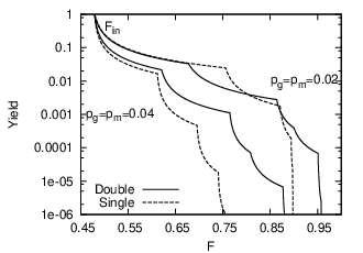
where $n_{\mathcal{A}}(F,F_{\textrm{ch}})$ denotes the minimum number of rounds which is required to achieve the fidelity $F$, $p_{\mathcal{A}}(\mathbf{F}^{(n-1)})$ denotes the probability to pass the purification procedure at the round $n$, as given in Eqs. (6) and (9), and $N_{\mathcal{A}}$ denotes the number of EPR pairs consumed at each round ($N_{\mathcal{S}}=2$ and $N_{\mathcal{D}}=3$). We plot in Fig. 6 the yield $Y_{\mathcal{A}}(F,F_{\rm ch}=0.8)$ as a function of the target fidelity $F$ for each protocol with $p_{g}=p_{m}=0.02$ (upper curves) and $p_{g}=p_{m}=0.04$ (lower curves). With less noisy local operations ($p_{g}=p_{m}=0.02$), both schemes provide comparable yields to achieve a target fidelity $F\approx 0.9$, where the numbers of rounds are $n_{\mathcal{S}}=4$ (single) and $n_{\mathcal{D}}=2$ (double). On the other hand, even when noisier local operations ($p_{g}=p_{m}=0.04$) are used, the double-selection scheme still provides a reasonable yield to achieve a target fidelity $F\approx 0.9$, where $n_{\mathcal{S}}=16$ and $n_{\mathcal{D}}=4$. Since the double-selection scheme uses three EPR pairs at each round, it may be thought to cost more resources than the single-selection scheme with two EPR pairs at each round. However, this is not the case. As shown in the above, the double-selection scheme provides a comparable or even better yield. This is because the double-selection scheme increases the fidelity of EPR pairs considerably faster than the single-selection scheme. In the case of the double selection, an additional EPR pair is worth enough to enhance the fidelity of purified states, as discussed in the following.

We here discuss the optimality of the double selection in the first order of the errors. We first consider an upper bound on the fidelity of purified states by general arguments. Then, it will be shown that the double selection really saturates this upper bound in the low noise regime.

While purification protocols contain many imperfect local operations, we can reasonably derive an upper bound on the fidelity in the first order by noting the errors introduced by the final two gate operations applied on the source EPR pair. Here we assume that the local operations for purification are implemented by bilateral two-qubit Clifford gates and measurements. (One-qubit gates may be absorbed into relevant two-qubit gates and local reference frames.) Specifically, consider a purification protocol with a combination of two bilateral C-Not gates at the final step, as shown in Fig. 7. We inspect these final C-Not gate operations in the Alice’s site to observe the undetectable errors left on the output state of the source qubit (s). (The same argument is made in the Bob’s site.) Passing through this set of the final gates, the preceding errors on the source qubit (s) are propagated to either or both of the ancilla qubits (a1) and (a2). Thus these preceding errors are all regarded to be detectable, that is an optimal purification protocol is expected to remove them by post-selection after the measurements of the ancillas. The upper bound on the fidelity is rather determined by some of the errors introduced by the final two gates themselves (black stars in Fig. 7) which are undetectable and thus unavoidable without leaving any information on the ancillas. As for the second final C-Not gate, only the $\sigma^{\rm(s)}_{3}\otimes\sigma^{\rm(a2)}_{0}$ error with the probability $p_{30}$ is undetectable, since it commutes with the final C-Not gate. On the other hand, all the $\sigma^{(\rm s)}_{i}\otimes\sigma^{\rm(a1)}_{0}$ errors of the final C-Not gate with the probabilities $p_{i0}$ are undetectable inevitably, since the output source qubit does not interact with ancillas afterward. By adding these undetectable errors due to the final two C-Not gates in the sites of Alice and Bob, the upper bound on the fidelity is placed in the first order of the errors as

Note here that the measurement error is not involved in considering the detectability of the errors with their propagation to the ancilla qubits. A portion of the right output state $\phi_{0}$ may be discarded by the errors in measuring the ancillas for verification. This slight reduction of the right state is cancelled by the renormalization after the post-selection except for the higher-order contributions. Thus the measurement error does not contribute to the upper bound in the first order. The precise upper bound will be lower than this first-order bound due to the higher-order contributions of the gate and measurement errors, though it is beyond our scope to estimate them analytically.

Another protocol may be considered by exchanging the final two C-Not gates in Fig. 7. (This is actually the case in the recurrence protocol considered so far when the purification procedure is finished at an even round.) Similarly, by observing the undetectable errors introduced by the final two C-Not gates, the upper bound on the fidelity is placed as

We note that these upper bounds in Eqs. (19) and (20) are valid even if the final two C-Not gates are set in the same direction (e.g., both the C-Not gates are controlled by the source qubit). In such configurations, some of the preceding errors on the source qubit become undetectable, commuting with the final two gates. Thus these configurations merely lower the fidelity.

These two upper bounds $F_{\rm upper}$ and $F^{\prime}_{\rm upper}$ coincide with each other for the uniform distribution of the gate errors $p_{ij}=p_{g}/15$, as adopted in calculating the maximum achievable fidelities of the single and double selections (Fig. 5). In general, the upper bound is given by ${\rm max}[F_{\rm upper},F^{\prime}_{\rm upper}]$ depending on the error distribution; in a recurrence protocol we should determine whether the purification procedure is finished at an even or odd round. We may also use other two-qubit Clifford gates instead of C-Not gates. Then, we obtain a similar upper bound with a suitable permutation among $p_{i0}$’s in Eq. (19) or Eq. (20), by considering which error of the second final gate is left commuting with the final gate.

We now show that the double selection really removes all the detectable errors in the first order, achieving the upper bound $F_{\rm upper}$. (We here adopt the uniform error distribution for definiteness.) The recurrence protocol considered so far, with either single or double selection, has the setup as shown in Fig. 7 with the proper exchange of the reference frames at each round. In the single selection (Fig. 1), the $\sigma_{1}$ and $\sigma_{2}$ ($\sigma_{2}$ and $\sigma_{3}$) errors on each ancilla EPR pair are detected by the $Z$ ($X$) measurement, while the $\sigma_{3}$ ($\sigma_{1}$) error is not detected. In the double selection (Fig. 2), the primary ancilla EPR pair is further verified with the secondary ancilla EPR pair so that all the errors on the primary ancilla EPR pair are detected in the first order. That is, all the detectable errors on the source EPR pair are certainly removed by the double selection through the interaction with the primary ancilla EPR pairs, as expected in deriving the upper bound. Therefore, the double-selection protocol achieves the upper bound in the first order as

This has been really confirmed by the numerical calculation in the low gate noise regime $p_{g}<0.02$, almost independently of the measurement error $p_{m}<0.05$.

On the other hand, as noted above, in the single selection (Fig. 1) the $\sigma_{3}$ ($\sigma_{1}$) error on the ancilla EPR pair cannot be detected by the $Z$ ($X$) measurement at an odd (even) round. Even in this case, all the errors before the second final C-Not gate are detected in the first order through the final two rounds, because the reference frames are properly exchanged at each round. However, some of the errors which have been excluded as detectable in deriving $F_{\rm upper}$ are actually left in the single-selection protocol. By counting these extra errors due to the final two C-Not gates in Fig. 7, we find that the maximum achievable fidelity of the single selection decreases as

As seen so far, the double selection is necessary and sufficient to remove fully the detectable first-order errors, saturating the upper bound on the fidelity in the low noise regime. There is no room for the triple (or more) selection to improve the fidelity except for the higher-order error contributions. In practice, as the triple selection itself introduces more errors with additional noisy operations, it will hardly improve the maximum achievable fidelity of the double selection.

References

- [1] C. H. Bennett, G. Brassard, C. Crépeau, R. Jozsa, A. Peres, and W. K. Wootters, Phys. Rev. Lett. 70, 1895 (1993).
- [2] C. H. Bennett and S. J. Wiesner, Phys. Rev. Lett. 69, 2881 (1992).
- [3] A. K. Ekert, Phys. Rev. Lett. 67, 661 (1991).
- [4] H.-J. Briegel, W. Dür, J. I. Cirac, and P. Zoller, Phys. Rev. Lett. 81, 5932 (1998); W. Dür, H.-J. Briegel, J. I. Cirac, and P. Zoller, Phys. Rev. A 59, 169 (1999).
- [5] R. Raussendorf and H.-J. Briegel, Phys. Rev. Lett. 86, 5188 (2001); R. Raussendorf, D. E. Browne, and H.-J. Briegel, Phys. Rev. A 68, 022312 (2003).
- [6] P. W. Shor, Proceedings of the 37th Annual Symposium on Foundations of Computer Science (IEEE Computer Society Press, Los Alamitos, CA, 1996), p. 56.
- [7] K. Chen and H.-K. Lo, Quant. Inf. Comp. 7, 689 (2007).
- [8] C. H. Bennett, G. Brassard, S. Popescu, B. Schumacher, J. A. Smolin, and W. K. Wootters, Phys. Rev. Lett. 76, 722 (1996); C. H. Bennett, D. P. DiVincenzo, J. A. Smolin, and W. K. Wootters, Phys. Rev. A 54, 3824 (1996).
- [9] D. Deutsch, A. Ekert, R. Jozsa, C. Macchiavello, S. Popescu, and A. Sanpera, Phys. Rev. Lett. 77, 2818 (1996).
- [10] M. Murao, M. B. Plenio, S. Popescu, V. Vedral, and P. L. Knight, Phys. Rev. A 57, R4075 (1998).
- [11] W. Dür, H. Aschauer, and H.-J. Briegel, Phys. Rev. Lett. 91, 107903 (2003); H. Aschauer, W. Dür, and H.-J. Briegel, Phys. Rev. A 71, 012319 (2005).
- [12] S. Glancy, E. Knill, and H. M. Vasconcelos, Phys. Rev. A 74, 032319 (2006).
- [13] C. Kruszynska, A. Miyake, H.-J. Briegel, and W. Dür, Phys. Rev. A 74, 052316 (2006).
- [14] A. Miyake and H.-J. Briegel, Phys. Rev. Lett. 95, 220501 (2005).
- [15] C. Kruszynska, S. Anders, W. Dür, and H.-J. Briegel, Phys. Rev. A 73, 062328 (2006).
- [16] A. Kay, Phys. Rev. A 77, 052319 (2008).
- [17] W. Dür and H.-J. Briegel, Rep. Prog. Phys. 70, 1381 (2007).
- [18] B. Eastin, Phys. Rev. A 75, 022301 (2007).
- [19] E. Knill, Nature 434, 39 (2005).
- [20] A. M. Steane, Phys. Rev. Lett. 78, 2252 (1997).
- [21] A. W. Cross, D. P. DiVincenzo, and B. M. Terhal, arXiv:0711.1556 (2007).
- [22] K. Fujii and K. Yamamoto, arXiv:0802.4137 (2008).