The Center of the Nilcoxeter and -Hecke Algebras
Abstract
We compute the dimension of the center of the 0-Hecke algebra and of the Nilcoxeter algebra using a calculus of diagrams on the Möbius band. In the case of the Nilcoxeter algebra, this calculus is shown to produce a basis for and the table of multiplication in this basis is shown to be trivial. We conjecture that a basis for can also be obtained in a specific way from this topological calculus.
1 Introduction
1.1 Generic Algebras
Given a Coxeter system and an associative commutative algebra with unity, we start by defining the generic algebra . This approach is taken from [5] and depends on parameters subject to the condition that and whenever and are conjugates in . is generated by elements for with relations
- 1.
if
- 2.
if
The two algebras of concern in this paper are both examples of this type of generic algebras with Coxeter group . Other important examples include the group algebra which is obtained by setting all and . Hecke algebras are also examples of this construction for and with and for all . For more on Coxeter groups and Hecke algebras see [6].
There is another set of relations equivalent to the ones above:
- 1.
if
- 2.
with the identity element. is in fact generated as an algebra by the and .
Any generic algebra with coxeter group , is generated by the following three relations:
- 1.
- 2.
for
- 3.
1.1.1 The Nilcoxeter Algebra
The Nilcoxeter algebra, which we denote , is an example of a generic algebra associated to where we set for all . This algebra first appeared in [1] in relation to the cohomology of flag varieties. It was also studied by Lascoux and Schützenberger [10], Macdonald [11], Fomin and Stanley [4] and others. Khovanov has shown in [7] that it categorifies the polynomial representation of the Weyl algebra and recent work by Khovanov and Lauda showed its relevance to the categorification of quantum groups [8]. In terms of the generators where for the transposition we have the following defining relations:
- 1.
- 2.
for
- 3.
We therefore also have
1.1.2 The 0-Hecke Algebra
The 0-Hecke algebra, denoted , is the Hecke algebra associated to with . Equivalently, it is the generic algebra where we have set and for all . That is, the third relation on the now becomes
This implies that
Norton studied the Hecke algebra of a Coxeter group at for all types in [12]; she classified the irreducible modules, described the decomposition of the algebra into left ideals as well as the Cartan invariants. In [2], Carter gave decomposition numbers for in the type case. Krob and Thibon gave a representation-theoretic interpretation of non-commutative algebras [9] and works by Duchamp, Hivert and Thibon [3] showed that the representations of in type categorify the ring of quasi-symmetric functions.
1.2 The Centers of Frobenius Algebras
We now derive some general facts about the centers of Frobenius algebras and then introduce a trace map which makes both and into Frobenius algebra. The facts here derived are crucial to our approach to describing the centers of and .
1.2.1 Symmetric Frobenius Algebras
To investigate the centers of Frobenius algebras, it is sometimes convenient to use a duality relation between the center and a quotient of by certain subgroups. In the case of symmetric Frobenius algebras, this subgroup is simply the commutator subgroup. Let be a Frobenius algebra over a field , its trace map and assume that is a symmetric algebra, meaning that for all . Denote by Hom the dual of . Then extends to an isomorphism of -bimodules:
Let denote the commutator subspace of : the space spanned by elements of the form for
Claim 1.1.
If is a symmetric Frobenius algebra, then
Proof.
Let
is well-defined:
since is a central element and is
symmetric.
is injective: since the map is an isomorphism and the map is an inclusion, the composition is injective.
Moreover, we have seen that the map factors through , which means that is
injective as well.
is surjective: let . Because
is surjective, its dual
must also be injective. We know from the isomorphism that for some . We must check that . Now, since , for all Hence
Since the trace is non-degenerate, this cannot be true for all unless . This is true for all as well, so we conclude that , with .
∎
1.2.2 Non-Symmetric Frobenius Algebras
We now look at the case when is not a symmetric Frobenius algebra. Since
is non-degenerate, one can define an involution such that . Using this involution, one can state a duality very similar to the one we have derived in the case of the symmetric Frobenius algebras.
Given the involution on , let us denote the ”twisted” commutator of and by . Similarly, let be the subalgebra of spanned by elements . We also define the twisted center of as follows:
Note that if then as well because
which means that since the involution is bijective. Moreover, if , we have
such that for a general , .
Claim 1.2.
With the above notation,
| (1.1) | |||||
| (1.2) |
Proof.
(1) The proof closely resembles the one for symmetric. Let
is well-defined:
since is central and
is injective: The proof is exactly as for symmetric.
is surjective: Let and . Then for some and for all We must verify that is in the center .
Since this is true for all and since is non-degenerate, then must vanish for
all , which means that is central.
(2) Let
is well-defined:
is injective: The proof is as before.
is surjective: We have as before and we need to check that
so that and . ∎
Note that and are no longer algebras, but vector spaces, both for and .
1.2.3 The Nilcoxeter and 0-Hecke Algebras as Non-Symmetric Frobenius Algebras
We can endow the -Hecke and Nilcoxeter algebras with a trace map, making them Frobenius algebras. Some of our constructions and arguments will be similar for both and . In these cases we denote either of them by , where is generated by , if we want to emphasize the dimension of our algebra, or simply by . Then is defined as if is maximal (the maximal permutation has length for the algebra on strands) and otherwise. With a slight abuse of notation, we now refer to or even as maximal when is maximal. The maximal is called .
Proposition 1.3.
is a non-degenerate trace map and makes and into Frobenius algebras.
Proof.
non-degenerate means that for any , there exist such that . The properties of the length function on and the multiplication rules derived in 1.1.1 and 1.1.2 imply that this is indeed the case.
∎
The -Hecke and Nilcoxeter algebras are not symmetric. However, one can define an involution on for both and :
It is clear the , for some , and that . It immediately follows that is maximal if and only if is maximal, so that if and only if . Hence, for all .
Acknowledgments: I would like to thank my advisor Mikhail Khovanov for his guidance as well as the NSF for supporting me while writing this paper through the grant DMS-0706924.
2 Topological Calculi of Diagrams
In order to determine the dimension of the center of our Frobenius algebra or , we make use of relation (1) of Claim 1.2 and determine the dimension of . A basis element of can be represented as a monotonic immersion of unit intervals in , subject to some relations. We can see this element as strings each going from a top position at to a bottom position at . A generator of is represented by the crossing of the and strings. The braid relations of allow us to change this diagram of strings using the third Reidemeister move () and to move far away crossings up and down with respect to each other ( for ). We read diagrams from top to bottom.

2.1 Diagrams on a Flat Band
A diagram like the one described above, a monotonic immersion of unit intervals in , can be used to represent a basis element of the symmetric group ring [] if we impose the usual Reidemeister moves as relations. By changing the relations appropriately, it can also represent a basis element of or . To or we assign a crossing of the and strands, to a product or we assign a crossing of the and strands followed by a crossing of the and strands and to a linear combination of basis elements we assign a formal sum of diagrams. The relations imposed are:
for a basis element of []:
- 1.
- 2.
for
- 3.
for a basis element of :
- 1.
- 2.
for
- 3.
and for a basis element of :
- 1.
- 2.
for
- 3.

Right multiplication of two basis elements then becomes the juxtaposition of the diagram for under the diagram for then rescaled to be in as shown in Figure 3.

To each word in there is assigned an element of and a diagram . In the Nilcoxeter algebra case, if is not reduced, then, and . In the -Hecke algebra case, for some reduced word and likewise, for some reduced diagram . Note that in general and are not equivalent words in . Moreover, because a reduced word in can be related to any other equivalent reduced word through the braid relations alone, diagrams in or corresponding to reduced words equivalent in are equivalent. Conversely, if two reduced diagrams are equivalent, then the reduced words to which they correspond are also equivalent in .
2.2 Diagrams on a Cylinder: The Quotients of the Nilcoxeter and 0-Hecke Algebras by Their Commutator Subgroups

Looking at diagrams on instead of imposes the new relation on as shown in Figure 4. This is equivalent to working in .

Figure 5 examplifies some of the consequences of this new relation for . Recall that is no longer an algebra but a vector space, both in the case and .
2.3 Diagrams on the Möbius band: The Quotients of the Nilcoxeter and 0-Hecke Algebras by Their Twisted Commutator Subgroups

A basis element of can be represented as a diagram of strings living on a Möbius band. On the Möbius band, a crossing , if last in the diagram, can be pushed around the band to become a crossing first in the diagram. Figure 6 shows how this can be done. Thus, as desired in . Indeed, on the Möbius band, this new relation corresponds exactly to the involution used to define the relation on . We typically represent these diagrams on a flat band, but one should mentally identify the top and bottom of the band in opposite directions so as to form a Möbius band. Figure 7 gives an example of Nilcoxeter diagrams which are equivalent on the Möbius band but not on a flat band or on a cylinder. The elements they represent are therefore identified in .

With the goal of understanding the center of , we classify these diagrams on the Möbius band. The cases and are very similar. We therefore carry out this classification in detail for and later give a summary of the corresponding results for .
3 Nilcoxeter Diagrams on the Möbius band
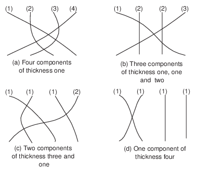
To begin our study of diagrams on the Möbius band, we fix some notation. First note that on the Möbius band, as well as on the cylinder, these strings could actually be any number of immersed circles. Each circle is called a component of the diagram and the number of times a single immersed circle goes around the Möbius band, i.e. the degree of that immersion, is called the thickness of that component. The sum of the individual thicknesses of the components of a diagram is , the thickness of the diagram. Figure 8 shows four diagrams of thickness four that decompose into components of different thicknesses. In general, one can see that a diagram of thickness with no crossing must consist of components each of thickness ; one of the components having both top and bottom positions 1 and , another positions 2 and , etc. The diagram corresponding to the image of in , the diagram with the maximum number of crossings, must consist of components each of thickness ; one component having top position 1 and bottom position , anothe top position 2 and bottom position , etc.
We now want to introduce the notion of a path . A path is defined in a specific component of a diagram . If has thickness and has thickness , we define as a sequence where is the top position of the strand of after going around the Möbius band times starting at . We always consider this sequence and all statements made about it should be understood as such. Figure 9 gives an example of a path for the central component of thickness four of this composite diagram of total thickness six. The starting position of this path is
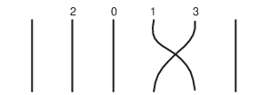
For each component , this sequence is determined by once is chosen. Hence, two paths in the same component can only differ by an integer , the lag of one path behind the other such that .
3.1 Prime Diagrams
A prime diagram is a diagram consisting of a single component. We will see that there is a unique prime diagram of thickness for each .
3.1.1 The Minimum Number of Crossings of a Prime Diagram
First, let us look at the minimal number of crossings such a diagram must have. If, instead of being on the Möbius band, we were on a simple cylinder , the minimal condition for the strands to be connected, to be part of the same component, would be clear: the diagram would have to correspond to an -cycle in , in particular, it would need to have at least the possible crossings ,…. In fact, it needs to have exactly each possible crossing once since on the cylinder, two strings are part of the same component if and only if they cross exactly once. Similarly, since the string with top position and the one with bottom position are already part of the same component in a diagram on the Möbius band, one can quickly see that on the Möbius band, a diagram of thickness needs one of or for each to be connected. The minimum number of crossings required is therefore .
3.1.2 The Exact Number of Crossings of a Prime Diagram
We need the following result to determine the maximum number of crossings that a non-zero prime diagram can have.
Proposition 3.1.
A diagram on the Möbius band is zero if and only if there are more than one crossing between two fixed paths.
Proof.
The first implication is clear: if there are two consecutive crossings for some in , then these two crossings must occur between the same two paths. Conversely, given two paths and , one can see them as being both “on top” of the other strands of for each . One can then slide a crossing occuring between these two paths around the Möbius band to the next or previous . The only obstacle to doing this is if there is already a crossing between these paths at this , in which case we have two consecutive crossings and If there are two crossings between these two paths occuring at different , one can then move one of them around the Möbius band until they are consecutive and annihilate the diagram. Figure 10 shows how this is done for a specific example.

∎
We have already shown that in order for to be prime, it must have at least crossings. We now check that this is actually the maximum number of crossings a prime diagram of thickness can have if it is to be non-zero.
Proposition 3.2.
A prime diagram of thickness has exactly crossings
Proof.
Let us fix a component . We want to look at (unordered) pairs of paths in , but some pairs are redundant. For instance, in Figure 9, we would like the two pairs of paths and to be equivalent. We therefore consider pairs of paths modulo relative starting points, that is we impose the relation
for some integer (remember that we are working ). Note that if lags on by , then lags on by . Since we are looking at unordered pairs and since any two pairs with the same lag are equivalent by the above relation, any pair of paths such that is equivalent to any pair such that since then . The pairs of paths modulo relative starting points are therefore indexed by an integer . In our example of Figure 9, we thus have a total of classes of pairs of paths, those which have a lag of or equivalently of such as , and those which have a lag of such as .
Remember that when the same pair of paths intersects twice, the diagram is zero. Moreover, a crossing belongs to a pair of paths if and only if it also belongs to all equivalent pairs. Thus, there can be only one crossing per equivalence class of pairs of paths
for the component to be non-zero. Since there are equivalence classes of pairs of paths, there can be a maximum of crossings within a component of thickness for the diagram to be non-zero.
In this section, we are concerned with prime diagrams, so now let =. For a prime diagram of odd thickness , the maximum number of crossings we have just derived , the minimum number of crossings previously derived, and the Proposition is proved. For of even thickness , we will show that cannot actually realize this maximum of crossings; it has either no more than crossings or is zero, which completes the proof of Proposition 3.2.
In fact, we show that a non-zero even prime diagram cannot have a middle crossing . First, note that the paths and , never intersect iff
and
for all (again, we consider both 2k and 2k+1 as integers ). Now, assume that contains no middle crossing and consider the paths . Since no strand ever crosses the middle point of the diagram, we have
and
such that and and , do not intersect. Having at least one class of pairs of paths which do not intersect, such a diagram has a maximum of crossings. Assume then that does contain a middle crossing . Without loss of generality, assume that is the top crossing of the diagram and consider the same paths . Now, since these paths cross immediately, . Suppose that these paths do not intersect again, then
and
for . But we know that
which is a contradiction. Therefore, (p,p’) must intersect more than once and is zero. ∎
3.1.3 The Crossings of a Prime Diagram
We have now shown that a prime diagram of thickness must have exactly crossings. Moreover, we know that these crossings are exactly or for each . In any case, each appears at most once, which allows us to push all of the crossings to the left side of the diagram and thus assume that the crossings are exactly for . Indeed, to see this first assume inductively that all , for , have already been pushed to the left side. We can do this since there is at most one crossing that could prevent from being moved. If there is a crossing above or below , the latter is free to be pushed in the other direction and if there is no then the crossing can be pushed either up or down the Möbius band to become . Consider now what could block . Everything to its right has already been pushed, so only above or below it can block it. It is therefore free to be pushed in the other direction. Therefore, from now on when we think of a prime diagram, we always represent it with its crossings being in some order. It remains to show that these diagrams are in fact all equal in .
3.1.4 Uniqueness of Prime Diagrams
Lemma 3.3.
for all
Proof.
First, let us look at the case when is a cyclic permutation. Fix . Now,
since for . More generally, if we have any diagram for , then
because in fact so that for unless is odd and . Then , but we still have
that for since for so that (*) still holds. Diagramatically, we have taken the top crossing and pushed it onto the right side of the diagram, where it is free to be pushed to the top again. We can then push it back to the bottom left side of the diagram. Hence the Lemma holds for a cyclic permutation. Figure 11 shows how this is done for a simple example.

Now let us compose a permutation with a transposition . Since we already know that this diagram is invariant under cyclic permutations of its crossings, we can actually assume that . If , and commute and we are done. Without loss of generality, assume therefore that . Let be such that . So
using the fact that it is invariant under cyclic permutations. Thus this diagram is in fact invariant under all permutations ∎
This Lemma now allows us to conclude that there is exactly one prime diagram of thickness for each . This diagram can be represented as .
3.2 Composite Diagrams
We now need to see how prime diagrams can be combined into non-zero composite diagrams. At first glance, there seems to be a number of ways to combine diagrams. Observe that, given two diagram and with the same prime components , it is always possible to go from to via an isotopy. Indeed, given that there is no under and overcrossings, one can first consider that is on top and place it where one wants, then do the same with and thus simply rearrange the components of as they are in . This isotopy, however, might very well go through zero in if . In fact, we know that if the second Reidemeister move is used, then it does go through zero, and we also know that this move is the only one which changes the number of crossings. Therefore, given isotopic diagrams and , if has more crossings than , then . Thus all non-zero diagrams in with the same prime components have the same number of crossings and that number is the minimum of the isotopy class. Note that such a minimum must exist and that the corresponding diagram, having no two paths crossing more than once since it is minimal, is non-zero.
Note also that the relations on these diagrams being local, any relation on a prime component continue to hold when the component is combined in a composite diagram.
3.2.1 Combining Even Prime Diagrams

Consider a diagram with even prime components of respective thicknesses . Since even prime diagrams have no middle crossings, we can combine and by either nesting inside , which means having at positions both on top and bottom and at positions or vice versa. Neither of these two arrangements will add crossings between and : if has crossings and has crossings and has crossings in either arrangement, which are therefore both minimal. Let be the diagram with in the center and the one with in the center. Then an isotopy from to requires the second Reidemeister moves which creates double crossings and the isotopy therefore goes through zero. Hence, and are distinct non-zero diagrams in .

3.2.2 Combining Odd and Even Components
Next, given a component (prime or composite) of total odd thickness with crossings, and even prime components , with crossings respectively, the minimal arragements have no intercomponent crossings: they have crossings. These arrangements all involve in the center, disjoint from the even components, which are split each in the middle around . If are all distinct, then there are arrangements of this type. By the same argument as in the case of two even diagrams, there is no isotopy between these arrangements that does not require the second Reidemeister move, so these diagrams are in fact distinct. Figure 14 is an example of such a minimal arrangement. Since has odd thickness and thus cannot be split in its middle, if it is not in the center, then it is also not disjoint from the even components. The corresponding diagram is then not minimal and is therefore zero.

3.2.3 Combining Odd Prime Diagrams
Let us now see how to combine two odd diagrams of thicknesses respectively into a diagram . To try to find a combination, one can start by numbering of the top positions of with numbers in a certain color. These would be the top position for the strands of . First note that once these top positions for are chosen, the bottom ones are determined. Indeed, if the number was assigned to the top position of , then the number is assigned to the bottom position . We call this assignment from , There seems to be many ways one can choose the positions of and in , but we will see that there is in fact a unique choice that makes non-zero.
Lemma 3.4.
There is a unique non-zero diagram with prime components of respective thicknesses .
Proof.
We describe an arrangement and then argue that it is the unique one with the minimum number of crossings. Without loss of generality, assume that
Let be the total thickness of . We build the diagram component by component. Let be the diagram of thickness with prime components obtained after the step of this procedure. The following assignment functions are the ones yielding the unique minimal diagram :
and
which means that we keep the previous composite in the center and give the edge positions.

First, we want to minimize the number of extra crossings of a component with itself. If possible, it is clear that a minimal diagram is one where the placement of each component does not add crossings between strands of the same component. If is not monotonic, extra crossings might be created, while none are added if is monotonic. Therefore, monotonic assignment functions create minimal diagrams. Note that for each component of thickness , if then and are equivalent on the Möbius band. Indeed, diagrams which are reflections of each other are seen to be the same by rotating the Möbius band. We therefore only consider strictly increasing assignment functions . Moreover, all assignment functions for a prime component which do not increase the number of crossings within itself are equivalent since all diagrams of with the minimal number of crossings are equivalent.

We also want to minimize crossings between and , which means that we want to avoid alternating positions,ie. situations like
which add intercomponent crossings. For a component of thickness in a diagram of total thickness , the botttom position is the same as the top position whenever
When this is not true, we have additional intercomponent crossings. Therefore, minimizing the crossings means that we want one component in the center and one on the outside of the diagram, each symmetric in their assignment.

Inductively, we see that in any diagram, there is one strand per odd component crossing the center line of the diagram. Therefore, if is placed as the outside component in , there are crossings between and , since is composed of odd prime components and one strand for each of these prime components will cross the strands of . Now, an odd component cannot really be split in two and placed on the outside because of the symmetry requirement. Placing it on the outside therefore implies taking the first and last position, both top and bottom to minimize crossings. The remaining position has bottom position assignment if it has top assignment . being an odd prime component, we know that, in the standard representation of this diagram, the strand having top position has bottom position in and the one having bottom position has top position . This means that in , if , the strand having top position in will cross times and the one with bottom position in will cross times for a total of
times. Now, since we have ordered the components such that
Therefore, placing the (thickest) prime odd component as the outside component always yields a minimal diagram. It remains to see whether the diagram is invariant under the choice of , the position in of the middle position of . This can be seen by pushing the crossing around the Möbius band so that it becomes . The diagram thus becomes exactly the diagram with . Doing the opposite, we get the diagram with , and so we see that is invariant under the choice of . There is therefore a unique diagram on the Möbius band with prime components . ∎
This completes the classification of Nilcoxeter diagrams on the Möbius band. We have learned that there is a unique prime diagram of thickness for each , that there is a unique diagram with only odd prime components and that in general, the number of arrangements depends on the number of even prime components of each thickness.
4 The Center of the Nilcoxeter Algebra
4.1 The Dimension of the Center
We have now enumerated all the possible arrangements of prime components into composite diagrams. Given even prime components , of them with thickness and odd prime components , one can make exactly distinct non-zero diagrams with this prime decomposition. We can now count the number of non-zero diagrams of thickness in , each of which is a basis element of . This number is also the dimension of the center of :
where is the number of even parts in and
For instance, for we have partitions
and the formula gives us
A more interesting case is where we have partitions
The formula then gives us
Here the partition gives us two distinct diagrams.
4.2 A Basis for the Center
We now know the dimension of the center of , but we would also like to have a basis for this center. Recall that we used the fact that
and that this isomorphism is given by the trace map . Therefore, we just need to find the dual of the diagrams we counted in the previous section. First, given an element , we call complementary to if , . Note that for this is equivalent to which also means that there is a unique complementary for each
Now, we need to find the element of corresponding to a basis element of . Since the distinct diagrams of thickness formed a basis for the vector space , their corresponding elements in are also linearly independent and therefore form a linear basis for . The element of corresponding to a given basis element is such that for any with , being the projection map. To find these elements of , we first need to find the elements of the coset of corresponding to a given element of . The element of we want is then the sum of the complementary elements of the elements of that coset. Here is an example for . Take the identity element in represented by three non-intersecting strands on the Möbius band. Its coset in is just itself: . Its complementary element is , our first basis element for . Conversely, the coset of is again just and its complementary element is the identity , our second basis element. Now let us consider . Its coset is since is equivalent to in . Their complementary elements are and respectively. Our third basis element is therefore . This ends our computation of the basis of for . See Figure 18 for the diagrams corresponding to this computation.

The Nilcoxeter algebra is a graded algebra with the grading given by the length function on . Equivalently, the grading of a basis element is given by the number of crosssings in its corresponding diagram. Note that the process described above to find a basis for yields a homogeneous basis since every element of the coset of an element of has the same length, or the same number of crossings.
4.3 Multiplication in the Center of
We would now like to know what the multiplication table looks like in the basis we have described in the previous section.
Lemma 4.1.
Every diagram corresponding to a basis element of other than has a vertical line as its first or last strand. Equivalently, a basis element of other than cannot have both and in its expression.
Proof.
First, let us look at a non-zero diagram on the Möbius band corresponding to a partition of which has at least one even part. Then, we know that one of these even prime diagrams is on the outside of and disjoint from its other components. We also know that all the elements in the coset of this prime even diagram have at least one such vertical strand as either their first or last strand. Since this even component is disjoint from all the other components of the diagram, this vertical strand clearly remains in all elements of the coset of . Figure 19 shows this for all the diagrams in the coset corresponding to the partition

We now look at a non-zero diagram on the Möbius band which is composed solely of odd prime components. Since is not the diagram for one of its prime components has thickness greater than one. Let the thickest prime component of have thickness Remember from the classification of these diagram that this means that this component must be the component occupying positions and both at the top and at the bottom of the diagram. This is true for any diagram equivalent to . Once again, every diagram of an odd prime component must have a vertical strand at position 1 or . This is true also of in since occupies positions 1 and both at the top and bottom of the diagram. Figure 20 shows that this is true in the case of the diagrams corresponding to the partition . ∎

Proposition 4.2.
The multiplication table for the center of in the basis described above is trivial.
Proof.
This vertical strand in every element of the cosets of our basis elements means that their complement must have either a strand going from top position to bottom position or from top position to bottom position , depending on whether the vertical strand is at position or , since has both of these diagonals. Since every basis element of is a sum of such complements, every diagram appearing in any basis element of has such a diagonal.
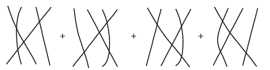
Multiplying two elements with the opposite diagonals obviously yields a non-minimal, and therefore zero, diagram since the strand in the product corresponding to these diagonals crosses every other strand twice.

If we multiply two elements with the same diagonal, we also have a trivial diagram. Indeed, remember that if two strands cross more than once, the diagram is zero. Since this diagonal strand crosses all other strands in the first element and does not remain vertical in the second because of the full diagonal of this second diagram, it must cross at least one strand twice.

Hence, the product of any basis element by any element other than the identity is zero and the multiplication table of is trivial as claimed.
∎
5 The Center of the 0-Hecke Algebra
5.1 0-Hecke Diagrams on the Möbius band
The classification of diagrams on the Möbius band band is identical to that of diagrams. All of the arguments of Section 3 go through for . Everytime a diagram was eliminated for being zero in , it is eliminated for not being minimal in . Zero diagrams in correspond exactly to non-minimal diagrams in . Non-zero diagrams which are equivalent in are also equivalent in and non-minimal diagrams which are equivalent in are equivalent in . Hence, the vector spaces for and are isomorphic and their bases are represented by the same diagrams on the Möbius band.
Therefore, the dimensions of the centers of and are the same:
where is the number of even parts in and
5.2 A Basis for the Center
Finding the basis for the center of corresponding to our basis for is more complex than in the case of the Nilcoxeter algebra. In that previous case, it was easy to see what linear combination of diagrams would complement any diagram representing a given basis element of . In other words, given a basis element , we needed to find an element such that for any with . This was simply the sum of the complements of all such .
Because of the relation
the coset of an element of tends to be much bigger for than for . To generate all of the elements of this coset, one needs to first generate all diagrams which are equivalent on the Möbius band, just as was done for . Then, use the above relation to double crossings and again generate all equivalent diagrams. Repeat this process until all the new diagrams are redundant. This algorithm generates redundant diagrams which should be ignored.
Then, an element of may have more than one complement. However, note that a diagram in can only have one complement with a given number of crossings. It then becomes clear that a simple sum of complements like the one we had for will not do; one needs a more complicated linear combination of them. Figure 24 gives the answer for

References
- [1] J.N. Bernstein, I.M. Gelfand, and S.I. Gelfand. Schubert cells and cohomology of the spaces . Russian Math. Surveys, 28:1–26, 1973.
- [2] R.W. Carter. Representation theory of the 0-Hecke algebra. J. Algebra, 104:89–103, 1986.
- [3] G. Duchamp, F. Hivert, and J.-Y. Thibon. Noncommutative symmetric functions VI: Free quasi-symmetric functions and related algebras, 2001.
- [4] S. Fomin and R.P. Stanley. Schubert polynomials and the nilCoxeter algebra. Advances in Math., 103:196–207, 1994.
- [5] James E. Humphrey. Reflection Groups and Coxeter Groups, volume 29 of Cambridge studies in advanced mathematics. Cambridge University Press, Cambridge,UK, 1990.
- [6] D. Kazhdan and G. Lusztig. Representations of Coxeter groups and Hecke algebras. Invent. Math., 53:165–184, 1979.
- [7] M. Khovanov. Nilcoxeter algebras categorify the Weyl algebra. COMM.ALGEBRA 29, 11:5033, 2001.
- [8] M. Khovanov and A. D. Lauda. A diagrammatic approach to categorification of quantum groups i, 2008.
- [9] D. Krob and J.-Y. Thibon. Noncommutative symmetric functions IV. quantum linear groups and hecke algebras at . J. Algebraic Combin., 6:339–376, 1997.
- [10] A. Lascoux and M.-P. Schützenberger. Fonctorialit’e des polynômes de Schubert\lx@bibnewblockIn Proceedings of the AMS Special Session on Invariant Theory, Vol. 88 (Denton,Texas, 1986), pages 585–595, Providence, RI, 1987. Amer. Math. Soc.
- [11] I.G. Macdonald. Notes on Schubert polynomials. Université du Québec à Montréal, Montréal,QC, Canada, 1991.
- [12] P.N. Norton. 0-Hecke algebras. J. Austral. Math. Soc., A27:337–357, 1979.