跳到论文正文
W Papers独立论文阅读器 arXiv:0811.2545 论文正文 计算阅读时间 · 0%
引用这篇论文根据当前论文元数据生成,正式投稿前建议核对。


License: arXiv.org perpetual non-exclusive license
arXiv:0811.2545v1 [math.DS] 16 Nov 2008

Expanding MeasuresThanks: Work carried out at the Federal University of Bahia, and IMPA. Partially supported by CNPq, PROCAD/CAPES, IMPA and PRONEX - Dynamical Systems

Vilton Pinheiro Address: Departamento de Matemática, Universidade Federal da Bahia
Av. Ademar de Barros s/n, 40170-110 Salvador, Brazil.
Email address: viltonj@ufba.br
Date: August 24, 2026
Abstract.

We prove that any C1+αC^{1+\alpha} transformation, possibly with a (non-flat) critical or singular region, admits an invariant probability measure absolutely continuous with respect to any expanding measure whose Jacobian satisfies a mild distortion condition. This is an extension to arbitrary dimension of a famous theorem of Keller [37] for maps of the interval with negative Schwarzian derivative.

We also show how to construct an induced Markov map FF such that every expanding probability of the initial transformation lifts to an invariant probability of FF. The induced time is bounded at each point by the corresponding first hyperbolic time (the first time the dynamics exhibits hyperbolic behavior). In particular, FF may be used to study decay of correlations and others statistical properties of the initial map, relative to any expanding probability.

1. Introduction

In this work we propose a general construction of Markov structures for non-uniformly expanding transformations. A distinctive feature is that these Markov structures capture all trajectories with expanding behavior.

In particular, we are able to use them to prove existence of ergodic invariant measures absolutely continuous with respect to any expanding reference measure with Hölder continuous Jacobian. In the special case when Lebesgue measure is the reference, this yields the physical measures of the transformation. Our Markov structures open the way for further development of the ergodic theory of this class of systems. In this direction, we construct Markov transformations induced from the original one, and we prove that any expanding invariant measure of the initial map lifts to invariant measure of these Markov transformations.

Markov partitions were the principal tool for analyzing the qualitative behavior of uniformly hyperbolic (Axiom A) or even uniformly expanding systems (see [56]). For uniformly hyperbolic dynamics, the systematic introduction of these partitions was due to Sinai [57, 58, 59] and Bowen [12, 13] and became a key technical tool in the ergodic theory of uniformly hyperbolic/expanding systems (see [14]). Sinai, Ruelle, Bowen used Markov partitions to associate these dynamical systems with symbolic ones, prove existence and uniqueness of equilibrium states, and several other properties, in a neighborhood of every transitive hyperbolic set. Recall that a Markov partition for a map f:Λ→Λf:\Lambda\to\Lambda is a cover 𝒫={P1,⋯,Ps}\mathcal{P}=\{P_{1},\cdots,P_{s}\} of Λ\Lambda satisfying

  • (a)

    int​Pi∩int​Pj=∅\mbox{int}P_{i}\cap\mbox{int}P_{j}=\emptyset if i≠ji\neq j;

  • (b)

    if f⁡(Pj)∩int​Pi≠∅f(P_{j})\cap\mbox{int}P_{i}\neq\emptyset then f⁡(Pj)⊃Pif(P_{j})\supset P_{i}.

Our setting is much more general than the classical family of uniformly expanding maps. Indeed we assume our systems to be non-uniformly expanding. In this setting one can not expect, in general, the existence of a classical finite Markov partition as there exist parts of the system that spend arbitrarily large time to present some expanding behavior. Nevertheless, we shall prove the existence of a quite similar partition that will be called an induced Markov partition. An induced Markov partition is an at most countable cover 𝒫={P1,P2,P3,⋯}\mathcal{P}=\{P_{1},P_{2},P_{3},\cdots\} of Λ\Lambda satisfying

  • (a)

    int​Pi∩int​Pj=∅\mbox{int}P_{i}\cap\mbox{int}P_{j}=\emptyset if i≠ji\neq j;

  • (b)

    for each PjP_{j} there is a Rj≥1R_{j}\geq 1 such that

    • (b.1)

      if ℓ<Rj\ell<R_{j} and fℓ​(Pj)∩int​Pi≠∅f^{\ell}(P_{j})\cap\mbox{int}P_{i}\neq\emptyset then fℓ​(Pj)⊂Pif^{\ell}(P_{j})\subset P_{i};

    • (b.2)

      if fRj​(Pj)∩int​Pi≠∅f^{R_{j}}(P_{j})\cap\mbox{int}P_{i}\neq\emptyset then fRj​(Pj)⊃Pif^{R_{j}}(P_{j})\supset P_{i}.

Let us be more precise about the kind of systems we will deal with in this paper. Formal statements will appear later. Let f:M→Mf:M\to M be a C1+αC^{1+\alpha} transformation outside some critical/singular set 𝒞⊂M\mathcal{C}\subset M (the case 𝒞=∅\mathcal{C}=\emptyset is a possibility). A positively invariant set ℋ⊂M\mathcal{H}\subset M is called expanding if every point x∈ℋx\in\mathcal{H} satisfies

lim supn→∞1n​∑i=0n−1log⁡‖(D​f​(fi​(x)))−1‖−1>0\limsup_{n\to\infty}\frac{1}{n}\sum_{i=0}^{n-1}\log\|(Df(f^{i}(x)))^{-1}\|^{-1}>0 (1)

and if ℋ\mathcal{H} satisfies the condition of slow approximation to the critical set, i.e., for each ε>0\varepsilon>0 there is a δ>0\delta>0 such that

lim supn→+∞1n∑j=0n−1−logdistδ(fj(x),𝒞)≤ε\limsup_{n\to+\infty}\frac{1}{n}\sum_{j=0}^{n-1}-\log\mbox{dist}_{\delta}(f^{j}(x),\mathcal{C})\leq\varepsilon (2)

for every x∈ℋx\in\mathcal{H}, where distδ⁡(x,𝒞)\operatorname{dist}_{\delta}(x,\mathcal{C}) denote the δ\delta-truncated distance from xx to 𝒞\mathcal{C} defined as distδ⁡(x,𝒞)=dist⁡(x,𝒞)\operatorname{dist}_{\delta}(x,\mathcal{C})=\operatorname{dist}(x,\mathcal{C}) if dist⁡(x,𝒞)≤δ\operatorname{dist}(x,\mathcal{C})\leq\delta and distδ⁡(x,𝒞)=1\operatorname{dist}_{\delta}(x,\mathcal{C})=1 otherwise.

A probability measure is called expanding if there is an expanding set ℋ\mathcal{H} such that μ⁡(ℋ)=1\mu(\mathcal{H})=1. If ff is a C1+αC^{1+\alpha} endomorphism then any invariant measure satisfying (1) almost everywhere is automatically an expanding measure (Corollary 10.3).

Given any expanding set ℋ\mathcal{H}, we construct an induced Markov partition 𝒫\mathcal{P} of ℋ\mathcal{H} with respect to ff (or an iterate of it). Associated to this partition there is an induced map

F:Λ→Λ,F⁡(x)=fR⁡(x)​(x),F:\Lambda\to\Lambda,\,\,\,\,F(x)=f^{R(x)}(x),

which is Markov, with an appropriate upper bound on the inducing time.

Given any reference measure ν\nu which gives positive weight to ℋ\mathcal{H}, we can use the induced Markov map to construct ff-invariant probabilities absolutely continuous with respect to ν\nu, and study decay of correlations and others statistical properties.

A crucial point to be noted is that every ff-invariant measure μ\mu that gives positive weight to ℋ\mathcal{H} can be lifted to the level of the induced map (the induced map does not depend on the measure μ\mu).

We also give several examples of expanding measures and applications of these results.

1.1. Statement of main results

Let MM be a compact Riemannian manifold of dimension d≥1d\geq 1 and f:M→Mf:M\to M a map defined on MM.

The map ff is called non-flat if it is a local C1+C^{1+} ( i.e., C1+αC^{1+\alpha} with α>0\alpha>0 ) diffeomorphism in the whole manifold except in a non-degenerate critical/singular set 𝒞⊂M\mathcal{C}\subset{M}. We say that 𝒞⊂M\mathcal{C}\subset{M} is a non-degenerate critical/singular set if ∃β,B>0\exists\beta,B>0 such that the following two conditions hold.

  1. (C.1)

    1B​d​i​s​t​(x,𝒞)β≤‖D​f​(x)​v‖‖v‖≤B​d​i​s​t​(x,𝒞)−β\displaystyle{\frac{1}{B}dist(x,\mathcal{C})^{\beta}\leq\frac{\|Df(x)v\|}{\|v\|}\leq B\,dist(x,\mathcal{C})^{-\beta}} for all v∈Tx​Mv\in T_{x}{M}.

For every x,y∈M∖𝒞x,y\in{M}\setminus\mathcal{C} with d​i​s​t​(x,y)<d​i​s​t​(x,𝒞)/2dist(x,y)<dist(x,\mathcal{C})/2 we have

  1. (C.2)

    |log⁡‖D​f​(x)−1‖−log⁡‖D​f​(y)−1‖|≤Bd​i​s​t​(x,𝒞)β​d​i​s​t​(x,y)\displaystyle{\left|\log\|Df(x)^{-1}\|-\log\|Df(y)^{-1}\|\>\right|\leq\frac{B}{dist(x,\mathcal{C})^{\beta}}dist(x,y)}.

If d​i​m​(M)=1dim({M})=1 and ff satisfies the usual one dimensional definition of non-flatness (see [41]), then it also satisfies the definition given above.

In the whole paper, a measure will be a countable additive measure defined on the Borel sets. A measure μ\mu is called ff-non-singular if f∗​μ≪μf_{*}\mu\ll\mu, where f∗​μf_{*}\mu (=μ∘f−1=\mu\circ f^{-1}) is the push-forward of μ\mu by ff.

Let ff be a non-flat map with critical/singular set 𝒞⊂M\mathcal{C}\subset M. A finite measure μ\mu is called ff-non-flat if it is ff-non-singular, μ⁡(𝒞)=0\mu(\mathcal{C})=0, Jμ​f​(x)J_{\mu}f(x) is well defined and positive for μ\mu-almost every x∈Mx\in M, and for μ\mu-almost every x,y∈M∖𝒞x,y\in{M}\setminus\mathcal{C} with d​i​s​t​(x,y)<d​i​s​t​(x,𝒞)/2dist(x,y)<dist(x,\mathcal{C})/2 we have

|log⁡Jμ​f​(x)Jμ​f​(y)|≤Bdist⁡(x,𝒞)β​dist⁡(x,y).\displaystyle{\left|\log\frac{J_{\mu}f(x)}{J_{\mu}f(y)}\>\right|\leq\frac{B}{\operatorname{dist}(x,\mathcal{C})^{\beta}}\operatorname{dist}(x,y)}.

1.1.1. Expanding sets and measures

Definition 1.1.

A positively invariant set ℋ⊂M\mathcal{H}\subset{M} (i.e., f⁡(ℋ)⊂ℋf(\mathcal{H})\subset\mathcal{H}) is called λ\lambda-expanding, λ≥0\lambda\geq 0, if

lim supn→∞1n​∑i=0n−1log⁡‖(D​f​(fi​(x)))−1‖−1>λ,\limsup_{n\to\infty}\frac{1}{n}\sum_{i=0}^{n-1}\log\|(Df(f^{i}(x)))^{-1}\|^{-1}>\lambda, (3)

for every x∈ℋx\in\mathcal{H}, and ℋ\mathcal{H} satisfies the slow approximation condition, i.e., for each ε>0\varepsilon>0 there is a δ>0\delta>0 such that (2) holds for every x∈ℋx\in\mathcal{H}.

An expanding set is a positively invariant set but, in general, it is not a compact one. In the one-dimensional case (3) reduces to the Lyapunov exponent of ff on xx to be bigger than λ\lambda, i.e.,

lim supn→∞1n​∑i=0n−1log⁡|f′​(fn​(x))|=lim supn→∞|(fn)′​(x)|>λ.\limsup_{n\to\infty}\frac{1}{n}\sum_{i=0}^{n-1}\log|f^{\prime}(f^{n}(x))|=\limsup_{n\to\infty}|(f^{n})^{\prime}(x)|>\lambda.
Definition 1.2 (Expanding measures).

We call a measure μ\mu (non necessarily invariant) a λ\lambda-expanding measure (with respect to ff) if μ\mu is ff-non-singular and there exists a λ\lambda-expanding set ℋ\mathcal{H} such that μ⁡(M∖ℋ)=0\mu(M\setminus\mathcal{H})=0.

Theorem A (Existence of absolutely continuous invariant measures).

Let f:M→Mf:M\to M be a non-flat map. If μ\mu is a ff-non-flat λ\lambda-expanding measure, λ>0\lambda>0, then there exists a finite collection of μ\mu absolutely continuous ergodic ff-invariant probabilities such that μ\mu-almost every point in MM belongs to the basin of one of these probabilities.

Recall that the basin of measure η\eta is the set ℬ⁡(η)\mathcal{B}(\eta) of the points x∈Mx\in M such that

limn→+∞1n​∑j=0n−1φ∘fj​(x)=∫φ​𝑑η,\lim_{n\to+\infty}\frac{1}{n}\sum_{j=0}^{n-1}\varphi\circ f^{j}(x)=\int\varphi d\eta,

for every continuous function φ:M→ℝ\varphi:M\to{\mathbb{R}}.

1.1.2. Markov partitions

Let f:U→Uf:U\to U a measurable map defined on a Borel set UU of a compact, separable metric space XX. A countable collection 𝒫={P1,P2,P3​…}\mathcal{P}=\{P_{1},P_{2},P_{3}...\} of Borel subsets of UU is called a Markov partition if

  1. (1)

    int​(Pi)∩int​(Pj)=∅\mbox{int}(P_{i})\cap\mbox{int}(P_{j})=\emptyset if i≠ji\neq j;

  2. (2)

    if f⁡(Pi)∩int​(Pj)≠∅f(P_{i})\cap\mbox{int}(P_{j})\neq\emptyset then f⁡(Pi)⊃int​(Pj)f(P_{i})\supset\mbox{int}(P_{j});

  3. (3)

    #{f(Pi)\#\{f(P_{i}) ; i∈ℕ}<∞i\in{\mathbb{N}}\}<\infty;

  4. (4)

    f|Pif|_{P_{i}} is a homeomorphism and it can be extended to a homeomorphism sending Pi¯\overline{P_{i}} onto f⁡(Pi)¯\overline{f(P_{i})};

  5. (5)

    limndiameter​(𝒫n​(x))=0\lim_{n}\mbox{diameter}(\mathcal{P}_{n}(x))=0 ∀x∈⋂n≥0f−n​(⋃iPi)\forall x\in\bigcap_{n\geq 0}f^{-n}\big(\bigcup_{i}P_{i}\big),

where 𝒫n​(x)\mathcal{P}_{n}(x) == {y\{y ; 𝒫⁡(fj​(y))=𝒫⁡(fj​(x))\mathcal{P}(f^{j}(y))=\mathcal{P}(f^{j}(x)) ∀ 0≤j≤n}\forall\,0\leq j\leq n\} and 𝒫⁡(x)\mathcal{P}(x) denotes the element of 𝒫\mathcal{P} that contains xx.

Definition 1.3 (Induced Markov partition).

A countable collection 𝒫={P1,P2,P3​…}\mathcal{P}=\{P_{1},P_{2},P_{3}...\} of Borel subsets of UU is called a induced Markov partition if it satisfies all conditions of a Markov partition except the second one which has to be substituted by the following

  1. (2)

    for each Pi∈𝒫P_{i}\in\mathcal{P} there is a Ri≥1R_{i}\geq 1 such that

    1. (2.1)

      if ℓ<Ri\ell<R_{i} and int​(fn​(Pi))∩int​(Pj)≠∅\mbox{int}(f^{n}(P_{i}))\cap\mbox{int}(P_{j})\neq\emptyset then int​(fn​(Pi))\mbox{int}(f^{n}(P_{i})) ⊂\subset int​(Pj)\mbox{int}(P_{j}) or int​(fn​(Pi))\mbox{int}(f^{n}(P_{i})) ⊃\supset int​(Pj)\mbox{int}(P_{j});

    2. (2.2)

      if fRi​(Pi)∩int​(Pj)≠∅f^{R_{i}}(P_{i})\cap\mbox{int}(P_{j})\neq\emptyset then fRi​(Pi)⊃int​(Pj)f^{R_{i}}(P_{i})\supset\mbox{int}(P_{j}).

Definition 1.4 (Markov map).

The pair (F,𝒫)(F,\mathcal{P}), where 𝒫\mathcal{P} is a Markov partition of F:U→UF:U\to U, is called a Markov map defined on UU. If F⁡(P)=UF(P)=U ∀P∈𝒫\forall\,P\in\mathcal{P}, (F,𝒫)(F,\mathcal{P}) is called a full Markov map.

Note that if (F,𝒫)(F,\mathcal{P}) is a full Markov map defined on an open set UU then the elements of 𝒫\mathcal{P} are open sets (because F⁡(P)=UF(P)=U and F|PF|_{P} is a homeomorphism ∀P∈𝒫\forall\,P\in\mathcal{P}).

Consider a measurable map f:M→Mf:M\to M from MM to MM (or, more in general, from the metric space XX to XX).

Definition 1.5 (Induced Markov map).

A Markov map (F,𝒫)(F,\mathcal{P}) defined on UU is called a induced Markov map for ff on UU if is there is a function R:U→ℕ={0,1,2,3,…}R:U\to{\mathbb{N}}=\{0,1,2,3,...\} (called inducing time) such that {R≥1}=⋃P∈𝒫P\{R\geq 1\}=\bigcup_{P\in\mathcal{P}}P, R|PR|_{P} is constant ∀P∈𝒫\forall\,P\in\mathcal{P} and F​(x)=fR⁡(x)​(x)F(x)=f^{R(x)}(x) ∀x∈U\forall\,x\in U.

If an induced Markov map (F,𝒫)(F,\mathcal{P}) is a full Markov map, we call (F,𝒫)(F,\mathcal{P}) an induced full Markov map.

Given an induced Markov map (F,𝒫)(F,\mathcal{P}), an ergodic ff-invariant probability μ\mu is said liftable to FF if there exists FF-invariant finite measure ν≪μ\nu\ll\mu such that

μ=∑P∈𝒫∑j=0R⁡(P)−1f∗j​(ν|P),\mu=\sum_{P\in\mathcal{P}}\sum_{j=0}^{R(P)-1}f_{\ast}^{j}\left(\nu|_{P}\right),

where RR is the inducing time of FF, ν|P\nu|_{P} denotes the measure given by ν|P​(A)=ν⁡(A∩P)\nu|_{P}(A)=\nu(A\cap P) and f∗jf_{*}^{j} is the push-forward by fjf^{j}.

Definition 1.6 (Markov structure).

A Markov structure for a set U⊂MU\subset M (or XX) is an at most countable collection 𝔉={(Fi,𝒫i)}i\mathfrak{F}=\{(F_{i},\mathcal{P}_{i})\}_{i} of induced Markov maps such that if μ\mu is an ergodic ff-invariant probability with μ⁡(U)=1\mu(U)=1 then ∃(Fi,𝒫i)∈𝔉\exists(F_{i},\mathcal{P}_{i})\in\mathfrak{F} such that μ\mu is liftable to FiF_{i}.

Theorem B (Markov structure for an expanding set).

Every λ\lambda-expanding set with λ>0\lambda>0 admits a finite Markov structure 𝔉={(F1,𝒫1),…,(Fs,𝒫s)}\mathfrak{F}=\{(F_{1},\mathcal{P}_{1}),...,(F_{s},\mathcal{P}_{s})\}. Furthermore, each (Fi,𝒫i)∈𝔉(F_{i},\mathcal{P}_{i})\in\mathfrak{F} is a full Markov map defined on some topological open ball UiU_{i} (also the elements of 𝒫i\mathcal{P}_{i} are topological open balls).

See Theorem 5 for a more complete version of this Theorem B.

As an expanding set ℋ\mathcal{H} is positively invariant, it follows from Theorem B that every ergodic ff-invariant probability having μ⁡(ℋ)>0\mu(\mathcal{H})>0 is liftable to one of the full induced Markov map F1,…,FsF_{1},...,F_{s} given by the Theorem B.

We say that a Borel set AA is an essentially open set if  interior​(A)¯⊃A\overline{\mbox{interior}(A)}\supset A, that is, the closure of the interior of AA contains AA. The theorem below shows that any expanding set ℋ\mathcal{H} admits a Markov structure composed by a single induced Markov map (F,𝒫)(F,\mathcal{P}) with 𝒫\mathcal{P} being a collection of essentially open sets.

Theorem C (Global expanding induced Markov map).

If ℋ\mathcal{H} is a λ\lambda-expanding set with λ>0\lambda>0 then there exist ℓ≥1\ell\geq 1 and ε0>0\varepsilon_{0}>0 such that for every 0<ε<ε00<\varepsilon<\varepsilon_{0} there are an induced Markov map (F,𝒫)(F,\mathcal{P}), with inducing time RR, and a finite partition 𝒫0\mathcal{P}_{0} of MM by essentially open sets satisfying the following conditions.

  1. (i)

    sup{diameter(P)\sup\{\operatorname{diameter}(P) ; P∈𝒫}≤max{diameter(P)P\in\mathcal{P}\}\leq\max\{\operatorname{diameter}(P) ; P∈𝒫0}<εP\in\mathcal{P}_{0}\}<\varepsilon.

  2. (ii)

    For each Q∈𝒫Q\in\mathcal{P} there exists P∈𝒫0P\in\mathcal{P}_{0} such that int​(Q)⊂P\mbox{int}(Q)\subset P.

  3. (iii)

    F⁡(P)∈𝒫0F(P)\in\mathcal{P}_{0} ∀P∈𝒫\forall\,P\in\mathcal{P}(in particular, the elements of PP are essentially open sets).

  4. (iv)

    dist⁡(F⁡(x),F⁡(y))≥8​dist⁡(x,y)\operatorname{dist}(F(x),F(y))\geq 8\operatorname{dist}(x,y) ∀x,y∈P\forall\,x,y\in P and ∀P∈𝒫\forall\,P\in\mathcal{P};

  5. (v)

    For all x,y∈Px,y\in P, P∈𝒫P\in\mathcal{P} and 0≤n≤R⁡(P)0\leq n\leq R(P),

    dist(fn(x),fn(y))≤(e−λ/8)(R⁡(P)−n)dist(F(x),F(y)).\operatorname{dist}(f^{n}(x),f^{n}(y))\leq\big(e^{-\lambda/8}\big)^{(R(P)-n)}\operatorname{dist}(F(x),F(y)).
  6. (vi)

    If μ\mu is ff-non-flat measure (not necessarily invariant) with μ⁡(M∖ℋ)=0\mu(M\setminus\mathcal{H})=0 then ∃ρ>0\exists\,\rho>0 such that

    |log⁡Jμ​F​(x)Jμ​F​(y)|≤ρ​dist⁡(F⁡(x),F⁡(y)),\left|\log\frac{J_{\mu}F(x)}{J_{\mu}F(y)}\right|\leq\rho\operatorname{dist}(F(x),F(y)),

    for μ\mu almost every x,y∈Px,y\in P and ∀P∈𝒫\forall\,P\in\mathcal{P}.

  7. (vii)

    If μ\mu is an ergodic ff-invariant measure with μ⁡(ℋ)>0\mu(\mathcal{H})>0 then μ|⋂j≥0f−ℓ​j({R>0})\mu\big|_{\bigcap_{j\geq 0}f^{-\ell\,j}(\{R>0\})} is an invariant measure with respect to fℓf^{\ell}.

  8. (viii)

    There is a good relation between the tail of the partition and the tail of the hyperbolic times (see Section 8 for the definition), i.e.,

    {R>n}∩ℋ⊂ℋ∖⋃j=1nHℓ​j,\{R>n\}\cap\mathcal{H}\subset\mathcal{H}\setminus\bigcup_{j=1}^{n}{\mathrm{H}}_{\ell\,j},

    where Hi{\mathrm{H}}_{i} denotes the set of points having ii as a (e−λ/4,ε)(e^{-\lambda/4},\varepsilon)-hyperbolic time.

  9. (ix)

    Every ergodic ff-invariant probability μ\mu with μ⁡(ℋ)>0\mu(\mathcal{H})>0 is liftable to FF.

  10. (x)

    If ℋ\mathcal{H} is an uniformly expanding set (i.e., ℋ¯=ℋ\overline{\mathcal{H}}=\mathcal{H}, ℋ∩𝒞=∅\mathcal{H}\cap\mathcal{C}=\emptyset and ∃n≥1\exists\,n\geq 1 such that ‖(D​fn​(x))−1‖−1>1\big\|\big(Df^{n}(x)\big)^{-1}\big\|^{-1}>1 ∀x∈ℋ\forall\,x\in\mathcal{H}) then the partition 𝒫\mathcal{P} is finite.

We want to observe that in Section 5 we introduce the zooming sets (that generalizes the expanding sets) and the theorems above are corollaries of Theorems D, E and F for zooming sets.

A second note is that, if ff is a C1+C^{1+} endomorphism, 𝒫\mathcal{P} is an induced Markov partition of ℋ\mathcal{H}, with respect to fℓf^{\ell}, and the estimate of the item (viii) of Theorem C can be rewritten in a more direct dependence on the expansion (3) and on the recurrence to the critical region (2) (see Theorem 9).

1.2. Overview of the paper

In Section 2 we introduced the notion of nested sets adapted to the kind of pre-images we want to deal with (for example, pre-images with some contraction).

In Section 3 we study the ergodic components for non (necessarily) invariant measures for maps on metric spaces.

In Section 4 we obtain a statistical characterization of the liftable measures for a given induced map.

Although we are basically interested in expanding measures (Section 1.1), we weakened the expansion condition to permit more flexibility in the applications. For this we introduce the zooming measures in Section 5.

In Section 6 and 7 we show most of the results for zooming sets and measures. In particular the existence of induced Markovian maps for zooming sets (Theorem E and F) and the existence of an invariant measure ν≪μ\nu{\ll}\mu that is absolutely continuous with respect to a given zooming measure with some distortion control (Theorem D).

Section 8 is dedicated to the definition and properties of expanding measures, as well as to establish the connection between these measures with the zooming ones. The existence of an absolutely continuous invariant measure for a given expanding measure, the induced Markovian maps for expanding sets and so on are consequences of the analogous result for zooming measures and in this section we use the zooming results to get the expanding ones.

In Section 9 we give many examples of expanding and zooming sets and measures. We give also some applications of the results of the previous sections. In particular, we study the decay of correlations for general expanding measures.

Acknowledgments. We thank V. Araújo, P. Brandão A. Castro and K. Oliveira for comments and for useful conversations. We thanks also IMPA, Brazil, and Universidade do Porto, Portugal, for the hospitality (specially J. Alves, M. F. Carvalho and J. Rocha) and the opportunity to present and discuss this work. We are specially grateful to P. Varandas, M. Todd, M. Viana and J. Palis not only for useful conversations but also for the incentive.

2. Nested sets

The notion of nice interval, introduced by Martens in [40], is a useful tool in the theory of real and complex one-dimensional dynamical systems (see, for instance, [41, 51]). A nice interval is an open interval II such that the forward orbit 𝒪+​(∂I)\mathcal{O}^{+}(\partial I) of the boundary of II does not return to I, i.e., 𝒪+​(∂I)∩I=∅\mathcal{O}^{+}(\partial I)\cap I=\emptyset. Note that nice intervals are natural and easy to construct for interval maps. For instance, two consecutive points of a periodic orbit define a nice interval. Its main property is that there are no linked pre-images of a nice interval, that is, if I1I_{1} and I2I_{2} are sent homeomorphically onto an open nice interval II by fn1f^{n_{1}} and fn2f^{n_{2}} respectively then either I1∩I2=∅I_{1}\cap I_{2}=\emptyset, I1⊂I2I_{1}\subset I_{2} or I2⊂I1I_{2}\subset I_{1}.

In the multidimensional case, the boundary of topological open balls are connect topological manifolds and if a chaotic transitive dynamic is not much symmetric, it is natural to expect that this dynamic will spread these boundaries to the whole manifold, forbidding any “nice ball”. In general, the same seems true for any set whose the boundary is not totally disconnected.

In this section we present the abstract construction of nested sets. This reformulates and generalizes the concept of nice interval. In Section 5 we show their abundance in the presence of some expansion (see Lemma 5.12).

Let f:X→Xf:X\to X be a map defined on a complete, separable metric space XX. Fixed some K⊂XK\subset{X}, a set P⊂XP\subset X is called a regular pre-image of order n∈ℕn\in{\mathbb{N}} of KK if fnf^{n} sends PP homeomorphically onto KK. Denote the order of PP (with respect to KK) by ord⁡(P)\operatorname{ord}(P).

Let us fix in all Section 2 a collection ℰ0\mathcal{E}_{0} of connected open subsets of X{X} (for instance, ℰ0\mathcal{E}_{0} can be the collection {fn(Vn(x))\{f^{n}(V_{n}(x)) ; x∈Hnx\in{{\mathrm{H}}}_{n} and n∈ℕ}n\in{\mathbb{N}}\} of all hyperbolic balls of X{X}, see Proposition 8.2). For each n∈ℕn\in{\mathbb{N}} and V∈ℰ0V\in\mathcal{E}_{0} consider some collection ℰn​(V)\mathcal{E}_{n}(V) of regular pre-images of order nn of KK. Set ℰn=(ℰn​(V))V∈ℰ0\mathcal{E}_{n}=(\mathcal{E}_{n}(V))_{V\in\mathcal{E}_{0}}. We call the sequence ℰ=(ℰn)n\mathcal{E}=(\mathcal{E}_{n})_{n} a dynamically closed family of (regular) pre-images if fℓ​(E)∈ℰn−ℓf^{\ell}(E)\in\mathcal{E}_{n-\ell} ∀E∈ℰn\forall\,E\in\mathcal{E}_{n} and ∀ 0≤ℓ≤n\forall\,0\leq\ell\leq n. Given Q∈ℰnQ\in\mathcal{E}_{n} we denote fn|Qf^{n}|_{Q} by fQf^{Q} and we denote the ℰ\mathcal{E}-inverse branch of associated to QQ, (fn|Q)−1(f^{n}|_{Q})^{-1}, by f−Qf^{-Q}.

Let ℰ=(ℰn)n\mathcal{E}=(\mathcal{E}_{n})_{n} be a dynamically closed family of pre-images. A set PP is called an ℰ\mathcal{E}-pre-image of a set W⊂XW\subset{X} if there is n∈ℕn\in{\mathbb{N}} and Q∈ℰnQ\in\mathcal{E}_{n} such that W⊂fn​(Q)W\subset f^{n}(Q) and P=f−Q​(W)P=f^{-Q}(W).

Remark 2.1.

Two distinct ℰ\mathcal{E}-pre-images 𝒳1\mathcal{X}_{1} and 𝒳2\mathcal{X}_{2} of some set 𝒳⊂X\mathcal{X}\subset{X} having the same order cannot intersect. Indeed, write n=ord⁡(𝒳1)=ord⁡(𝒳2)n=\operatorname{ord}(\mathcal{X}_{1})=\operatorname{ord}(\mathcal{X}_{2}) and for each i∈{1,2}i\in\{1,2\} write 𝒳i=f−Qi​(𝒳)\mathcal{X}_{i}=f^{-Q_{i}}(\mathcal{X}), with Qi∈ℰnQ_{i}\in\mathcal{E}_{n}. Let Pj=f−Qj​(Q1∩Q2)P_{j}=f^{-Q_{j}}(Q_{1}\cap Q_{2}), for j=1,2j=1,2. It follows that P1∩P2⊃𝒳1∩𝒳2≠∅P_{1}\cap P_{2}\supset\mathcal{X}_{1}\cap\mathcal{X}_{2}\neq\emptyset. Of course P1≠P2P_{1}\neq P_{2}, otherwise 𝒳2\mathcal{X}_{2} == f−Q2​(𝒳)f^{-Q_{2}}(\mathcal{X}) == (fn|P2)−1​(𝒳)(f^{n}|_{P_{2}})^{-1}(\mathcal{X}) == (fn|P1)−1​(𝒳)(f^{n}|_{P_{1}})^{-1}(\mathcal{X}) == f−Q1​(𝒳)f^{-Q_{1}}(\mathcal{X}) == 𝒳1\mathcal{X}_{1}. Thus P1∩∂P2≠∅P_{1}\cap\partial P_{2}\neq\emptyset or P2∩∂P1≠∅P_{2}\cap\partial P_{1}\neq\emptyset. Assume that P1∩∂P2≠∅P_{1}\cap\partial P_{2}\neq\emptyset. So, ∅≠fn​(P1∩∂P2)⊂fn​(P1)∩∂(fn​(P2))⊂(Q1∩Q2)∩∂(Q1∩Q2)=∅\emptyset\neq f^{n}(P_{1}\cap\partial P_{2})\subset f^{n}(P_{1})\cap\partial\big(f^{n}(P_{2})\big)\subset(Q_{1}\cap Q_{2})\cap\partial\big(Q_{1}\cap Q_{2}\big)=\emptyset. An absurd.

Definition 2.2 (Linked sets).

We say that two open sets U1U_{1} and U2U_{2} are linked if both U1∖U2U_{1}\setminus U_{2} and U2∖U1U_{2}\setminus U_{1} are not empty sets.

Note that two connected open sets U1U_{1} and U2U_{2} are linked if and only if ∂U1∩U2\partial U_{1}\cap U_{2} and U1∩∂U2U_{1}\cap\partial U_{2} are not empty sets.

Definition 2.3 (ℰ\mathcal{E}-nested set).

A set VV is called ℰ\mathcal{E}-nested if VV is an open set and VV is not linked with any ℰ\mathcal{E}-pre-image of VV.

The fundamental property of a nested set is that any ℰ\mathcal{E}-pre-images P1P_{1} and P2P_{2} of it are not linked (see Corollary 2.6).

We can extend the concept of ℰ\mathcal{E}-nested set to a collection of sets in the following way.

Definition 2.4 (ℰ\mathcal{E}-nested collection of sets).

A collection 𝒜\mathcal{A} of open sets is called an ℰ\mathcal{E}-nested collection of sets if every A∈𝒜A\in\mathcal{A} is not linked with any ℰ\mathcal{E}-pre-image of an element of 𝒜\mathcal{A} with order bigger than zero. Precisely, if A1∈𝒜A_{1}\in\mathcal{A} and PP is an ℰ\mathcal{E}-pre-image of some A2∈𝒜A_{2}\in\mathcal{A}, then either A1A_{1} and PP are not linked or P=A2P=A_{2}.

It follows from the definition of an ℰ\mathcal{E}-nested collection of sets that every sub-collection of an ℰ\mathcal{E}-nested collection is also an ℰ\mathcal{E}-nested collection. In particular, each element of an ℰ\mathcal{E}-nested collection is an ℰ\mathcal{E}-nested set.

Lemma 2.5 (Main property of a nested collection).

If 𝒜\mathcal{A} is an ℰ\mathcal{E}-nested collection of open sets and P1P_{1} and P2P_{2} are ℰ\mathcal{E}-pre-images of two elements of 𝒜\mathcal{A} with ord⁡(P1)≠ord⁡(P2)\operatorname{ord}(P_{1})\neq\operatorname{ord}(P_{2}) then P1P_{1} and P2P_{2} are not linked.

Proof.

Let ℓj=ord⁡(Pj)\ell_{j}=\operatorname{ord}(P_{j}) for j=1,2j=1,2. We may assume that ℓ1<ℓ2\ell_{1}<\ell_{2} and, by contradiction, assume that P1P_{1} and P2P_{2} are linked. Let, for i=1,2i=1,2, pj∈Pj∩∂P3−jp_{j}\in P_{j}\cap\partial P_{3-j}, Qi∈ℰℓiQ_{i}\in\mathcal{E}_{\ell_{i}} and Ai∈𝒜A_{i}\in\mathcal{A} be such that Pi=f−Qi​(Ai)P_{i}=f^{-Q_{i}}(A_{i}). As ℰ\mathcal{E} is a dynamically closed family of pre-images of elements of ℰ0\mathcal{E}_{0}, Q=fℓ1​(Q2)∈ℰℓ2−ℓ1Q=f^{\ell_{1}}(Q_{2})\in\mathcal{E}_{\ell_{2}-\ell_{1}} and P=fℓ1​(P2)=f−Q​(A2)P=f^{\ell_{1}}(P_{2})=f^{-Q}(A_{2}) is an ℰ\mathcal{E}-pre-image of A2A_{2}. On the other hand fℓ1​(P1)=A1∈𝒜f^{\ell_{1}}(P_{1})=A_{1}\in\mathcal{A}. As fℓ1​(p1)∈fℓ1​(P1)∩∂(fℓ1​(P2))=A1∩∂Pf^{\ell_{1}}(p_{1})\in f^{\ell_{1}}(P_{1})\cap\partial\big(f^{\ell_{1}}(P_{2})\big)=A_{1}\cap\partial P and fℓ1​(p2)∈fℓ1​(P2)∩∂(fℓ1​(P1))=P∩∂A1f^{\ell_{1}}(p_{2})\in f^{\ell_{1}}(P_{2})\cap\partial\big(f^{\ell_{1}}(P_{1})\big)=P\cap\partial A_{1}, it follows that PP and A1A_{1} are linked, but this is impossible because 𝒜\mathcal{A} is ℰ\mathcal{E}-nested.

∎

Corollary 2.6 (Main property of a nested set).

If VV is an ℰ\mathcal{E}-nested set and P1P_{1} and P2P_{2} are ℰ\mathcal{E}-pre-images of VV then P1P_{1} and P2P_{2} are not linked. Furthermore,

  1. (1)

    if P1∩P2≠∅P_{1}\cap P_{2}\neq\emptyset then ord⁡(P1)≠ord⁡(P2)\operatorname{ord}(P_{1})\neq\operatorname{ord}(P_{2});

  2. (2)

    if P1⫋P2P_{1}\subsetneqq P_{2} with ord⁡(P1)<ord⁡(P2)\operatorname{ord}(P_{1})<\operatorname{ord}(P_{2}) then VV is contained in an ℰ\mathcal{E}-pre-image of itself with order bigger than zero,

    ford⁡(P2)−ord⁡(P1)​(V)⊂V.f^{\,\operatorname{ord}(P_{2})-\operatorname{ord}(P_{1})}(V)\subset V.
Proof.

Lets suppose that P1≠P2P_{1}\neq P_{2} are ℰ\mathcal{E}-pre-images of VV and set ℓj=ord⁡(Pj)\ell_{j}=\operatorname{ord}(P_{j}) for j=1,2j=1,2. By Remark 2.1, ℓ1≠ℓ2\ell_{1}\neq\ell_{2}. Thus, we may assume that ℓ1<ℓ2\ell_{1}<\ell_{2}. By Lemma 2.5 it follows that P1P_{1} and P2P_{2} are not linked.

Now, suppose in addition that P1⊂P2P_{1}\subset P_{2}. Then V=fℓ1​(P1)⊂fℓ1​(P2)V=f^{\ell_{1}}(P_{1})\subset f^{\ell_{1}}(P_{2}) (fℓ1​(P2)f^{\ell_{1}}(P_{2}) is an ℰ\mathcal{E}-pre-image of VV) and this will imply that fℓ2−ℓ1​(V)⊂fℓ2​(P2)=Vf^{\,\ell_{2}-\ell_{1}}(V)\subset f^{\ell_{2}}(P_{2})=V. ∎

2.1. Constructing nested sets

In this section (Section 2.1) let 𝒜\mathcal{A} be a collection of connected open sets such that the elements of 𝒜\mathcal{A} are not contained in any ℰ\mathcal{E}-pre-image of order bigger than zero of an element of 𝒜\mathcal{A}.

Refer to caption
Figure 1. A chain (P0,P1,P2,P3)(P_{0},P_{1},P_{2},P_{3}) of pre-images beginning in AA.

A finite sequence 𝒦=(P0,P1,⋯,Pn)\mathcal{K}=(P_{0},P_{1},\cdots,P_{n}) of ℰ\mathcal{E}-pre-images of elements of 𝒜\mathcal{A} is called a chain of pre-images of 𝒜\mathcal{A} beginning in A∈𝒜A\in\mathcal{A} (Figure 1) if

  1. (1)

    0<ord⁡(P0)≤⋯≤ord⁡(Pn−1)≤ord⁡(Pn)0<\operatorname{ord}(P_{0})\leq\cdots\leq\operatorname{ord}(P_{n-1})\leq\operatorname{ord}(P_{n});

  2. (2)

    AA and P0P_{0} are linked;

  3. (3)

    Pj−1P_{j-1} and PjP_{j} are linked ∀1≤j≤n\forall 1\leq j\leq n;

  4. (4)

    Pi≠PjP_{i}\neq P_{j} ∀i≠j\forall\,i\neq j.

Denote by c​hℰ​(A)ch_{\mathcal{E}}(A) the collection of all chain of pre-images of 𝒜\mathcal{A} beginning in A∈𝒜A\in\mathcal{A}. As the elements of 𝒜\mathcal{A} are connected and open, it is easy to check the following remark.

Remark 2.7.

If (P0,P1,⋯,Pn)∈c​hℰ​(A)(P_{0},P_{1},\cdots,P_{n})\in ch_{\mathcal{E}}(A), with A∈𝒜A\in\mathcal{A}, then ⋃j=n0n1Pj\bigcup_{j=n_{0}}^{n_{1}}P_{j} is a connected open set ∀ 0≤n0≤n1≤n\forall\,0\leq n_{0}\leq n_{1}\leq n.

For each A∈𝒜A\in\mathcal{A} define the open set

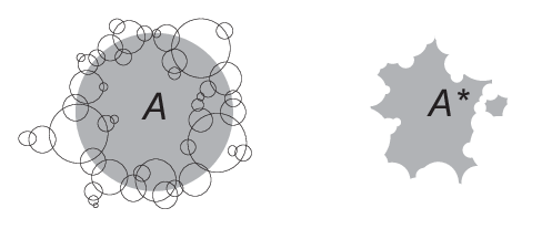
A⋆=A∖⋃(Pj)j∈c​hℰ​(A)⋃jPj¯.A^{\star}=A\setminus\,\overline{\bigcup_{(P_{j})_{j}\in ch_{\mathcal{E}}(A)}\bigcup_{j}P_{j}}. (4)
Refer to caption
Figure 2. On the left side it is shown a ball AA (in grey) and the boundaries of the pre-images of AA that belong to the chains. On the right side A⋆A^{\star} is shown.
Proposition 2.8 (An abstract construction of a nested collection).

For each A∈𝒜A\in\mathcal{A} such that A⋆≠∅A^{\star}\neq\emptyset choose a connected component A′A^{\prime} of A⋆A^{\star}. If 𝒜′={A′\mathcal{A}^{\prime}=\{A^{\prime} ; A∈𝒜A\in\mathcal{A} and A⋆≠∅}A^{\star}\neq\emptyset\} is not an empty collection then 𝒜′\mathcal{A}^{\prime} is an ℰ\mathcal{E}-nested collection of sets.

Proof.

Suppose that 𝒜′≠∅\mathcal{A}^{\prime}\neq\emptyset. By contradiction, assume that there exist A1,A2∈𝒜A_{1},A_{2}\in\mathcal{A} and a ℰ\mathcal{E}-pre-image PP of A2′A_{2}^{\prime} such that A1′A_{1}^{\prime} and PP are linked. So, as A1′A_{1}^{\prime} and PP are connected sets, ∃p∈P∩∂A1′\exists\,p\in P\cap\partial A_{1}^{\prime}. Let ℘=ord⁡(P)\wp=\operatorname{ord}(P) and let E∈ℰ℘E\in\mathcal{E}_{\wp} be such that P=f−E​(A2′)P=f^{-E}(A_{2}^{\prime}). Setting Q=f−E​(A2)Q=f^{-E}(A_{2}), we get P⊂QP\subset Q.

Claim.

Q⊂A1Q\subset A_{1}.

Proof.

First note that Q∩A1⊃Q∩A1′⊃P∩A1′≠∅Q\cap A_{1}\supset Q\cap A_{1}^{\prime}\supset P\cap A_{1}^{\prime}\neq\emptyset. On the other hand, if Q∩∂A1≠∅Q\cap\partial A_{1}\neq\emptyset, the unitary sequence (Q)(Q) will be a chain of ℰ\mathcal{E}-pre-images beginning in A1A_{1}, i.e., (Q)∈c​hℰ​(A1)(Q)\in ch_{\mathcal{E}}(A_{1}). But this is a contradiction to the definition of A1⋆A_{1}^{\star} because Q∩A1⋆⊃Q∩A1′≠∅Q\cap A_{1}^{\star}\supset Q\cap A_{1}^{\prime}\neq\emptyset. Thus, Q∩∂A1=∅Q\cap\partial A_{1}=\emptyset. As QQ and A1A_{1} are connected sets and Q∩A1⊃Q≠∅Q\cap A_{1}\supset Q\neq\emptyset, we get Q⊃A1Q\supset A_{1} or Q⊂A1Q\subset A_{1}. The first option is not possible because (by hypothesis) the elements of 𝒜\mathcal{A} are not contained in any ℰ\mathcal{E}-pre-image of order bigger than zero of an element of 𝒜\mathcal{A}. Therefore, Q⊂A1Q\subset A_{1}. ∎

Refer to caption
Figure 3.

As p∈∂A1′p\in\partial A_{1}^{\prime}, for a given ε>0\varepsilon>0 there exists a chain (Q0,⋯,Qn)∈c​hℰ​(A1)(Q_{0},\cdots,Q_{n})\in ch_{\mathcal{E}}(A_{1}) such that dist(p,∪j=0nQj)\operatorname{dist}(p,\cup_{j=0}^{n}Q_{j}) << ε\varepsilon. On the other hand, as PP and QQ are open sets and p∈P⊂Qp\in P\subset Q, taking ε\varepsilon small enough, P∩(∪j=0nQj)≠∅P\cap(\cup_{j=0}^{n}Q_{j})\neq\emptyset and so,

Qm∩Q⊃Qm∩P≠∅,Q_{m}\cap Q\supset Q_{m}\cap P\neq\emptyset, (5)

for some 1≤m≤n1\leq m\leq n. As Q0∪⋯∪QmQ_{0}\cup\cdots\cup Q_{m} is a connected set (Remark 2.7) and Q0∩(X∖Q)⊃Q0∩(X∖A1)≠∅Q_{0}\cap({X}\setminus Q)\supset Q_{0}\cap({X}\setminus A_{1})\neq\emptyset (because Q0Q_{0} and A1A_{1} are linked), there exists 0≤j≤m0\leq j\leq m such that Qj∩∂Q≠∅Q_{j}\cap\partial Q\neq\emptyset. Let ℓ=min{0≤j≤m\ell=\min\{0\leq j\leq m ; Qj∩Q≠∅}Q_{j}\cap Q\neq\emptyset\}.

We have two cases, either ord⁡(Qℓ)≤ord⁡(Q)\operatorname{ord}(Q_{\ell})\leq\operatorname{ord}(Q) or ord⁡(Qℓ)>ord⁡(Q)\operatorname{ord}(Q_{\ell})>\operatorname{ord}(Q). Suppose first that ord⁡(Qℓ)≤ord⁡(Q)\operatorname{ord}(Q_{\ell})\leq\operatorname{ord}(Q). By the minimality of ℓ\ell, Q≠QjQ\neq Q_{j} ∀ 0≤j≤ℓ\forall\,0\leq j\leq\ell. Thus, it is easy to check that 𝒦=(Q0,⋯,Qℓ,Q)∈c​hℰ​(A1)\mathcal{K}=(Q_{0},\cdots,Q_{\ell},Q)\in ch_{\mathcal{E}}(A_{1}). As Q∩A1⋆⊃Q∩A1′≠∅Q\cap A_{1}^{\star}\supset Q\cap A_{1}^{\prime}\neq\emptyset, the existence of the chain 𝒦\mathcal{K} is a contradiction to (4) and so, this case cannot occur. For the second case (ord⁡(Qℓ)>ord⁡(Q)\operatorname{ord}(Q_{\ell})>\operatorname{ord}(Q)), consider the sequence 𝒦=(f℘​(Qℓ),⋯,f℘​(Qm))\mathcal{K}=(f^{\wp}(Q_{\ell}),\cdots,f^{\wp}(Q_{m})). It is also easy to check that 𝒦∈c​hℰ​(A2)\mathcal{K}\in ch_{\mathcal{E}}(A_{2}) (note that, as f℘​(Q)=A2f^{\wp}(Q)=A_{2}, f℘​(Qℓ)∩∂A2=f℘​(Qℓ∩∂Q)≠∅f^{\wp}(Q_{\ell})\cap\partial A_{2}=f^{\wp}(Q_{\ell}\cap\partial Q)\neq\emptyset). But, as f℘​(P)=A2′⊂A2⋆f^{\wp}(P)=A_{2}^{\prime}\subset A_{2}^{\star}, it follows from (5) that f℘​(Qm)∩A2⋆⊃f℘​(Qm∩P)≠∅f^{\wp}(Q_{m})\cap A_{2}^{\star}\supset f^{\wp}(Q_{m}\cap P)\neq\emptyset, contradicting (4) again and concluding the proof. ∎

An easy way to assure the existence of nested sets (or collections) is to show that the chains have small diameter, where the diameter of a chain (Pj)j(P_{j})_{j} is defined as the diameter of ⋃jPj\bigcup_{j}P_{j}.

Corollary 2.9.

Let ε∈(0,1/2)\varepsilon\in(0,1/2) and let A=Br​(p)A=B_{r}(p) be a connected open ball with radius rr centered in p∈Xp\in X such that fn​(A)⊄Af^{n}(A)\not\subset A ∀n>0\forall\,n>0. If every chain of ℰ\mathcal{E}-pre-images of AA has diameter smaller than 2​ε​r2\varepsilon r then the set A⋆A^{\star}, given by (4) contains the ball Br⁡(1−2​ε)​(p)B_{r(1-2\varepsilon)}(p). Moreover, the connected component A′A^{\prime} of A⋆A^{\star} that contains pp is a ℰ\mathcal{E}-nested set containing Br⁡(1−2​ε)​(p)B_{r(1-2\varepsilon)}(p).

Proof.

Set 𝒜={A}\mathcal{A}=\{A\}. As fn​(A)⊄Af^{n}(A)\not\subset A ∀n>0\forall\,n>0, it follows that AA is not contained in any ℰ\mathcal{E}-pre-image of itself (with order bigger than zero). Let Γ\Gamma be the collection of all chains of ℰ\mathcal{E}-pre-images of AA. If (Pj)j∈Γ(P_{j})_{j}\in\Gamma then ⋃jPj\bigcup_{j}P_{j} is a connected open set intersecting ∂A\partial A with diameter smaller than 2​ε​r2\varepsilon r. Thus, ⋃jPj⊂B2​ε​r​(∂A)\bigcup_{j}P_{j}\subset B_{2\varepsilon r}(\partial A), ∀(Pj)j∈Γ\forall\,(P_{j})_{j}\in\Gamma. As a consequence, A⋆=A∖⋃(Pj)j∈Γ⋃jPj¯⊃A∖Bε​(∂A)¯⊃Br⁡(1−2​ε)​(p)A^{\star}=A\setminus\,\overline{\bigcup_{(P_{j})_{j}\in\Gamma}\bigcup_{j}P_{j}}\supset A\setminus\overline{B_{\varepsilon}(\partial A)}\supset B_{r(1-2\varepsilon)}(p) is a non-empty open set. Taking A′A^{\prime} as the connected component of A⋆A^{\star} that contains pp (and so, contains Br⁡(1−2​ε)​(p)B_{r(1-2\varepsilon)}(p)), it follows from Proposition 2.8 that A′A^{\prime} is a ℰ\mathcal{E}-nested set.∎

3. Ergodic components

Before constructing the Markov partition using the adapted nested sets, we need also some preliminary knowledge of the so called ergodic components for non (necessarily) invariant measures. This knowledge is important to assure good statistical properties for these nested sets with respect to the class of measures that we are working on.

Let μ\mu be a finite measure defined on the Borel sets of the compact, separable metric space X{X} and let f:X→Xf:X\to X be a measurable map. A subset U⊂XU\subset{X} is called an invariant set (with respect to ff) if f−1​(U)=Uf^{-1}(U)=U, and it is called a positively invariant set if f⁡(U)⊂Uf(U)\subset U.

Definition 3.1 (Ergodic components).

An invariant set UU with μ⁡(U)>0\mu(U)>0 is called an ergodic component (indeed, a μ\mu ergodic component with respect to ff), if it does not admit any smaller invariant subset with positive measure, that is, if V⊂UV\subset U is invariant, f−1​(V)=Vf^{-1}(V)=V, then either μ⁡(V)\mu(V) or μ⁡(U∖V)\mu(U\setminus V) is zero. The measure μ\mu is called ergodic if XX is an ergodic component.

We stress that in the definition of ergodic measure and ergodic components we are not assuming the invariance of the measure μ\mu with respect to ff. Let us give some examples of non-invariant ergodic measures.

Example 3.2.

Given any p∈X∖Fix​(f)p\in X\setminus\mbox{Fix}(f), the Dirac measure δp\delta_{p} is ergodic and non-invariant (Fix​(f)\mbox{Fix}(f) is the set of fixed points of ff). More in general, given a finite subset 𝒰⊂𝒪f−​(p)\mathcal{U}\subset\mathcal{O}_{f}^{-}(p) of the pre-orbit of a point p∈Xp\in X, let μ=1#​𝒰​∑q∈𝒰δq\mu=\frac{1}{\#\mathcal{U}}\sum_{q\in\mathcal{U}}\delta_{q}. If f−1​(𝒰)≠𝒰f^{-1}(\mathcal{U})\neq\mathcal{U} then μ\mu is an ergodic probability but not invariant.

Example 3.3.

Given an ergodic (not necessarily invariant) measure μ\mu, let Y⊂XY\subset X be such that μ⁡(Y)​μ​(f−1​(Y)∖Y)>0\mu(Y)\mu(f^{-1}(Y)\setminus Y)>0. Then μ|Y\mu|_{Y}, the restriction of μ\mu to YY, is non-invariant and ergodic.

Example 3.4.

By Martens [40], the Lebesgue measure is ergodic and non-invariant for every non-flat SS-unimodal map ff without a periodic attractor. In particular when ff is an infinitely renormalizable map the Lebesgue measure is ergodic but there is no absolutely continuous invariant measure (for multimodal maps, see Blokh-Lyubich [9, 10] and Vargas-van Strien [60]).

Following Milnor’s definition of attractor (indeed, minimal attractor [42]), a compact positively invariant set AA will be called a μ\mu-attractor, or for short, an attractor, if its basin of attraction ℬf​(A)={x∈X;ωf​(x)⊂A}\mathcal{B}_{f}({A})=\{x\in{X}\,{;}\,{{\omega}_{f}}(x)\subset A\} has positive measure and, in contrast, the basin of every positively invariant compact subset A′⫋AA^{\prime}\subsetneqq{A} has zero measure. Here, ωf​(x){{\omega}_{f}}(x) denotes the ω\omega-limit set of x∈Xx\in{X}.

A collection 𝒫\mathcal{P} of sets with positive measure is called a partition mod μ\mu of U⊂XU\subset{X} if this collection covers UU almost everywhere (μ⁡(U∖⋃P∈𝒫P)=0\mu(U\setminus\bigcup_{P\in\mathcal{P}}P)=0) and μ⁡(P∩Q)=0\mu(P\cap Q)=0 for every P,Q∈𝒫P,Q\in\mathcal{P} with P≠QP\neq Q. The diameter of a partition 𝒫\mathcal{P} is defined by diameter​(𝒫)\mbox{diameter}(\mathcal{P}) == sup{diameter(P)\sup\{\mbox{diameter}(P) ; P∈𝒫}.P\in\mathcal{P}\}.

Proposition 3.5 (Ergodic attractors).

Given an ergodic component U⊂XU\subset{X}, there exists a unique attractor A⊂XA\subset{X} that attracts almost every point of UU. Moreover, ωf​(x)=A{{\omega}_{f}}(x)=A for almost every point of UU.

Proof.

Let 𝒫1\mathcal{P}_{1} be any finite partition (mod μ\mu) of UU formed by open subsets and with diameter​(𝒫1)<1\mbox{diameter}(\mathcal{P}_{1})<1. We will construct by induction a sequence of partitions 𝒫1<𝒫2<…\mathcal{P}_{1}<\mathcal{P}_{2}<... of UU in the measure-theoretical sense. Thus, suppose that the collection 𝒫n−1\mathcal{P}_{n-1} has already been constructed. Set, for each P∈𝒫n−1P\in\mathcal{P}_{n-1}, UP={x∈U;ωf(x)∩P≠∅}U_{P}=\{x\in U\,{;}\,{{\omega}_{f}}(x)\cap P\neq\emptyset\}. As UU is an ergodic component and f−1​(UP)=UPf^{-1}(U_{P})=U_{P} (because ωf​(x)=ω⁡(f⁡(x)){{\omega}_{f}}(x)={\omega}(f(x)) ∀x\forall\,x), either UPU_{P} or U∖UPU\setminus U_{P} is a zero measure set.

Given P∈𝒫n−1P\in\mathcal{P}_{n-1}, we define a partition ℙP\mathbb{P}_{P} (mod μ\mu) of PP as follows. If μ⁡(UP)=0\mu(U_{P})=0, we set ℙP\mathbb{P}_{P} as the trivial refinement, i.e., ℙP={P}\mathbb{P}_{P}=\{P\}. On the other hand, if μ⁡(UP)>0\mu(U_{P})>0, we choose any ℙP\mathbb{P}_{P} in the collection of finite partitions (mod μ\mu) of P∈𝒫n−1P\in\mathcal{P}_{n-1} formed by open subset of PP with diameter smaller that 12​diameter​(P)\frac{1}{2}\mbox{diameter}(P) (see Lemma 10.1). Now, define

Pn={Q∈ℙP;P∈𝒫n−1}.P_{n}=\{Q\in\mathbb{P}_{P}\,{;}\,P\in\mathcal{P}_{n-1}\}.

For each n∈ℕn\in\mathbb{N}, set 𝒫n∗={P∈𝒫n;U∖UP\mathcal{P}_{n}^{*}=\{P\in\mathcal{P}_{n}\,{;}\,U\setminus U_{P} is a zero measure set}\} and Kn=⋃P∈𝒫n∗P¯K_{n}=\bigcup_{P\in\mathcal{P}_{n}^{*}}\overline{P}. As K1⊃K2⊃…⊃Kn⊃…K_{1}\supset K_{2}\supset...\supset K_{n}\supset... is a nested sequence of non-empty compact sets, A=⋂nKn{A}=\bigcap_{n}K_{n} is also a non-empty compact set. By construction, for almost every point x∈Ux\in U and ∀n∈ℕ\forall n\in\mathbb{N}, ωf​(x)⊂Kn{{\omega}_{f}}(x)\subset K_{n} and ωf​(x)∩P{{\omega}_{f}}(x)\cap P ∀P∈𝒫n∗\forall P\in\mathcal{P}_{n}^{*}. Moreover, as diameter​(P¯)<2−n\mbox{diameter}(\overline{P})<2^{-n} ∀P∈𝒫n∗\forall P\in\mathcal{P}_{n}^{*}, it follows that sup{dist⁡(y,𝒪f​(x));y∈A}≤2−n\sup\{\operatorname{dist}(y,\mathcal{O}_{f}(x))\,{;}\,y\in A\}\leq 2^{-n} and ωf​(x)⊂Kn⊂B2−n​(A)¯={p∈X;dist⁡(p,A)≤2−n}{{\omega}_{f}}(x)\subset K_{n}\subset\overline{B_{2^{-n}}(A)}=\{p\in{X}\,{;}\,\operatorname{dist}(p,A)\leq 2^{-n}\} for every n∈ℕn\in{\mathbb{N}} and almost every point x∈Ux\in U. Thus, ωf​(x)=A{{\omega}_{f}}(x)=A for μ\mu-almost every point x∈Ux\in U. ∎

Consider for each point xx of a positively invariant set U⊂XU\subset{X}, a subset 𝒰​(x)⊂𝒪+​(x)\mathcal{U}(x)\subset\mathcal{O}^{+}(x) of the positive orbit of xx.

Definition 3.6.

The collection 𝒰=(𝒰⁡(x))x∈U\mathcal{U}=(\mathcal{U}(x))_{x\in U} is called asymptotically invariant if for every x∈Ux\in U,

  1. (1)

    #⁡{j∈ℕ;fj​(x)∈𝒰⁡(x)}=∞\#\{j\in{\mathbb{N}}\,{;}\,f^{j}(x)\in\mathcal{U}(x)\}=\infty and

  2. (2)

    𝒰⁡(x)∩𝒪+​(fn​(x))=𝒰⁡(f⁡(x))∩𝒪+​(fn​(x))\mathcal{U}(x)\cap\mathcal{O}^{+}(f^{n}(x))=\mathcal{U}(f(x))\cap\mathcal{O}^{+}(f^{n}(x)) for every big n∈ℕn\in{\mathbb{N}}.

Definition 3.7 (ωf,𝒰{\omega}_{f,\mathcal{U}}).

Given an asymptotically invariant collection 𝒰=(𝒰⁡(x))x∈U\mathcal{U}=(\mathcal{U}(x))_{x\in U}, define for each xx the omega-𝒰\,\mathcal{U} limit set of xx (omega-𝒰\,\mathcal{U} of xx, for short), denoted by ωf,𝒰​(x){\omega}_{f,\mathcal{U}}(x), as the set of accumulation points of 𝒰⁡(x)\mathcal{U}(x) and, that is, the set of points p∈Xp\in{X} such that there is a sequence nj→+∞n_{j}\to+\infty satisfying 𝒰⁡(x)∋fnj​(x)→p\mathcal{U}(x)\ni f^{n_{j}}(x)\to p.

It is easy to check that ω𝒰​(x){\omega}_{\mathcal{U}}(x) is a non-empty compact set but not necessarily invariant.

We say that the asymptotically invariant collection 𝒰=(𝒰⁡(x))x∈U\mathcal{U}=(\mathcal{U}(x))_{x\in U} has positive frequency if lim sup1n#{1≤j≤n;fj(x)∈𝒰(x)}>0\limsup\frac{1}{n}\#\{1\leq j\leq n\,{;}\,f^{j}(x)\in\mathcal{U}(x)\}>0, for every x∈Ux\in U.

Definition 3.8 (ω+,f,𝒰{\omega}_{{}_{+},f,\mathcal{U}}).

If 𝒰\mathcal{U} is an asymptotically invariant collection with positive frequency, define ω+,f,𝒰(x){\omega}_{{}_{+},f,\mathcal{U}}(x), the set of 𝒰\mathcal{U}-frequently visited points of xx orbit, as the set of points p∈Xp\in{X} such that lim sup1n#{1≤j≤n;fj(x)∈𝒰(x)∩V}>0\limsup\frac{1}{n}\#\{1\leq j\leq n\,{;}\,f^{j}(x)\in\mathcal{U}(x)\cap V\}>0 for every neighborhood VV of pp.

Lemma 3.9.

Let 𝒰=(𝒰⁡(x))x∈U\mathcal{U}=(\mathcal{U}(x))_{x\in U} be an asymptotically invariant collection defined in an ergodic component UU and let A⊂XA\subset{X} be the attractor associated to UU. There is a compact set A𝒰⊂AA_{\mathcal{U}}\subset A such that ωf,𝒰​(x)=A𝒰{\omega}_{f,\mathcal{U}}(x)=A_{\mathcal{U}} for μ\mu-almost every x∈Ux\in U. Furthermore, if 𝒰\mathcal{U} has positive frequency then there is also a compact set A+,𝒰⊂A𝒰A_{{}_{+},\mathcal{U}}\subset A_{\mathcal{U}} such that ω+,f,𝒰(x)=A+,𝒰{\omega}_{{}_{+},f,\mathcal{U}}(x)=A_{{}_{+},\mathcal{U}} for μ\mu-almost every x∈Ux\in U.

Proof.

We construct the compact sets A𝒰{A}_{\mathcal{U}} and A+,𝒰{A}_{{}_{+},\mathcal{U}} in the same way we did for A{A} in the proof of Proposition 3.5. For A𝒰{A}_{\mathcal{U}} the only difference is that we have to change ωf​(x){{\omega}_{f}}(x) by ωf,𝒰​(x){\omega}_{f,\mathcal{U}}(x) in the proof. Note that the key property of ωf​(x){{\omega}_{f}}(x) used there is that ωf​(x)=ωf​(f⁡(x)){{\omega}_{f}}(x)={\omega_{f}}(f(x)) and we also have the same property for ωf,𝒰{\omega}_{f,\mathcal{U}}, i.e., ωf,𝒰​(x)=ωf,𝒰​(f⁡(x)){\omega}_{f,\mathcal{U}}(x)={\omega}_{f,\mathcal{U}}(f(x)).

For A+,𝒰{A}_{{}_{+},\mathcal{U}} we have, of course, to change in the proof ωf{{\omega}_{f}} by ω+,f,𝒰{\omega}_{{}_{+},f,\mathcal{U}} (again ω+,f,𝒰(x)=ω+,f,𝒰(f(x)){\omega}_{{}_{+},f,\mathcal{U}}(x)={\omega}_{{}_{+},f,\mathcal{U}}(f(x)) ∀x\forall\,x) and we have also to change the definition of the set UPU_{P}. For this we proceed as follows. Given a point x∈Ux\in U and a set K⊂XK\subset{X} denote the 𝒰\mathcal{U}-visit frequency of xx to KK by ϕK(x)=lim sup1n#{0≤j<n;fj(x)∈K∩𝒰(x)}\phi_{K}(x)=\limsup\frac{1}{n}\#\{0\leq j<n\,{;}\,f^{j}(x)\in K\cap\mathcal{U}(x)\}. Set, for each P∈𝒫n−1P\in\mathcal{P}_{n-1}, UP={x∈U;ϕP​(x)>0}U_{P}=\{x\in U\,{;}\,\phi_{P}(x)>0\}. As we are using lim sup\limsup in the definition of ϕK\phi_{K}, we get ϕK​(x)>0\phi_{K}(x)>0 or ϕX∖K​(x)>0\phi_{{X}\setminus K}(x)>0. This is important to ensure that Kn≠∅K_{n}\neq\emptyset ∀n\forall n (see proof of Proposition 3.5).

To finish the proof, we remark that every point of A+,𝒰=⋂nKn{A}_{{}_{+},\mathcal{U}}=\bigcap_{n}K_{n} is accumulated by the sequence {fn(x);n∈ℕ\{f^{n}(x)\,{;}\,n\in{\mathbb{N}} and fn(x)∈𝒰(x)}f^{n}(x)\in\mathcal{U}(x)\} for almost every point x∈Ux\in U and so, A+,𝒰{A}_{{}_{+},\mathcal{U}} is contained in A𝒰A_{\mathcal{U}} which is contained in A{A}. Moreover, if BB is an open set with B∩A+,𝒰≠∅B\cap{A}_{{}_{+},\mathcal{U}}\neq\emptyset then for any big nn there will be some element PP of 𝒫n∗\mathcal{P}^{*}_{n} contained in BB. Therefore, by construction, lim sup1n#{0≤j<n;fj(x)∈B∩𝒰(x)}≥lim sup1n#{0≤j<n;fj(x)∈P∩𝒰(x)}>0\limsup\frac{1}{n}\#\{0\leq j<n\,{;}\,f^{j}(x)\in B\cap\mathcal{U}(x)\}\geq\limsup\frac{1}{n}\#\{0\leq j<n\,{;}\,f^{j}(x)\in P\cap\mathcal{U}(x)\}>0. ∎

Refer to caption
Figure 4. UU is an ergodic component with its attractor AA and its omega-𝒰\,\mathcal{U} set A𝒰A_{\mathcal{U}}.

As defined in Section 5, a measure μ\mu is ff-non-singular if the pre-image by ff of any set with zero measure has also zero measure (f∗​μ≪μf_{*}\mu\ll\mu). The ergodic measures that appears in Example 3.2 and 3.3 are not in general ff-non-singular. The lemma below gives a way to construct new ff-non-singular ergodic measures.

Lemma 3.10.

If μ\mu is a ff-non-singular ergodic measure (not necessarily invariant) then 1μ⁡(E)μ|E\frac{1}{\mu(E)}\mu|_{{}_{E}} is a ff-non-singular ergodic probability whenever E⊂XE\subset X is a positively invariant Borel set with positive measure (i.e., f⁡(E)⊂Ef(E)\subset E and μ⁡(E)>0\mu(E)>0).

Proof.

As in Example 3.3, 1μ⁡(E)μ|E\frac{1}{\mu(E)}\mu|_{{}_{E}} is an ergodic probability. We need only to show that this probability is ff-non-singular. Given Y⊂XY\subset X, we have μ​(f−1​(Y)∩E)\mu(f^{-1}(Y)\cap E) ≤\leq μ⁡(f−1​(Y)∩f−1​(f⁡(E)))\mu(f^{-1}(Y)\cap f^{-1}(f(E))) == μ⁡(f−1​(Y∩f⁡(E)))\mu(f^{-1}(Y\cap f(E))). Thus, if μ|E(Y)=μ(Y∩E)=0\mu|_{{}_{E}}(Y)=\mu(Y\cap E)=0 then 0≤μ|E(f−1(Y))≤μ(f−1(Y∩f(E)))=00\leq\mu|_{{}_{E}}(f^{-1}(Y))\leq\mu(f^{-1}(Y\cap f(E)))=0 (because μ\mu is ff-non-singular). As a consequence, 1μ⁡(E)μ|E\frac{1}{\mu(E)}\mu|_{{}_{E}} is ff-non-singular.

∎

Lemma 3.11.

Let μ\mu be a finite measure. If there exists some δ>0\delta>0 such that every invariant set has μ\mu measure either zero or bigger than δ\delta, then X{X} can be decomposed into a finite number of μ\mu ergodic components.

Proof.

Let W1⊂XW_{1}\subset{X} be any invariant subset of X{X} (for example, W1=XW_{1}={X}) with non zero μ\mu measure and let ℱ⁡(W1)\mathcal{F}(W_{1}) be the collection of all invariant subsets U⊂W1U\subset W_{1} with μ\mu measure bigger than zero. Note that ℱ⁡(W1)\mathcal{F}(W_{1}) is non-empty, because W1∈ℱ⁡(W1)W_{1}\in\mathcal{F}(W_{1}). Let us consider the inclusion (mod μ\mu) as a partial order on ℱ⁡(W1)\mathcal{F}(W_{1}).

Claim.

Every totally ordered subset Γ⊂ℱ⁡(W1)\Gamma\subset\mathcal{F}(W_{1}) is finite. In particular, it has an upper bound.

Proof.

Otherwise there is an infinite sequence γ0⊃γ1⊃γ3⊃⋯\gamma_{0}\supset\gamma_{1}\supset\gamma_{3}\supset\cdots with μ⁡(γk∖γk+1)>0\mu(\gamma_{k}\setminus\gamma_{k+1})>0 ∀k\forall k. But as ∑kμ⁡(γk∖γk+1)=μ⁡(γ0)<∞\sum_{k}\mu(\gamma_{k}\setminus\gamma_{k+1})=\mu(\gamma_{0})<\infty, it follows that μ⁡(γk∖γk+1)<δ\mu(\gamma_{k}\setminus\gamma_{k+1})<\delta for kk big and this contradicts our hypothesis as every γk∖γk+1\gamma_{k}\setminus\gamma_{k+1} is an invariant set. ∎

From Zorn’s lemma, there exists a maximal element U1∈ℱ⁡(W1)U_{1}\in\mathcal{F}(W_{1}) and this is necessarily an ergodic component.

As W2=X∖U1W_{2}={X}\setminus U_{1} is an invariant set, either it has zero μ\mu measure or we can use the argument above to W2W_{2} and obtain a new ergodic component U2U_{2} inside X∖U1{X}\setminus U_{1}. Inductively, we can construct a collection of ergodic components U1,…,UrU_{1},...,U_{r} while μ⁡(X∖U1∪…∪Ur)>0\mu({X}\setminus U_{1}\cup...\cup U_{r})>0. But, as μ⁡(Uj)>δ\mu(U_{j})>\delta, this processes will stop and we will get the decomposition of X{X} into μ\mu ergodic components as desired.

∎

Proposition 3.12 (A criterion for ergodicity).

Let μ\mu be a ff-non-singular finite measure. If there exists some δ>0\delta>0 such that every positively invariant set has μ\mu measure either zero or bigger than δ\delta, then X{X} can be decomposed into a finite number of μ\mu ergodic components. Moreover, the attractor associated to each ergodic component has positive μ\mu measure.

Proof.

As every invariant set is positively invariant, it follows from Lemma 3.11 that X{X} can be decomposed into a finite number of μ\mu ergodic components.

From Proposition 3.5 each ergodic component UU of X{X} is the basin of some attractor A{A}. Let us, for instance, suppose that μ⁡(A)=0\mu({A})=0. In this case, one can choose an open neighborhood VV of A{A} such that μ⁡(V)<δ\mu(V)<\delta and an integer n0n_{0} such that μ⁡(U′)>0\mu(U^{\prime})>0, where U′={x∈U;fn(x)∈V∀n≥n0}U^{\prime}=\{x\in U\ {;}\ f^{n}(x)\in V\ \forall n\geq n_{0}\}. Note that μ⁡(fn0​(U′))>0\mu(f^{n_{0}}(U^{\prime}))>0 because μ\mu is ff-non-singular. As U′U^{\prime} is positively invariant, fn0​(U′)f^{n_{0}}(U^{\prime}) is a positively invariant set with 0<μ⁡(fn0​(U′))<μ⁡(V)<δ0<\mu(f^{n_{0}}(U^{\prime}))<\mu(V)<\delta, but this is impossible by ours hypothesis. So, μ⁡(A)>0\mu({A})>0 (indeed, μ⁡(A)>δ\mu({A})>\delta). ∎

We end this section relating the number of μ\mu ergodic components with respect to ff to the number of μ\mu ergodic components with respect to fkf^{k}.

Lemma 3.13.

Let μ\mu be a ff-non-singular finite measure. If UU is an ergodic component with respect to ff then UU can be partitioned in at most kk ergodic components with respect to fkf^{k}. Furthermore, if U1,U2⊂UU_{1},U_{2}\subset U are ergodic components with respect to fkf^{k} then U2=f−j​(U1)U_{2}=f^{-j}(U_{1}) (mod μ\mu) for some 0≤j<k0\leq j<k.

Proof.

First we will prove by induction that UU can be partitioned (mod μ\mu) in a finite number of ergodic components with respect to fkf^{k}. Of course this claim is true for k=1k=1. Thus, suppose by induction that for every 1≤j≤k−11\leq j\leq k-1 we can decompose UU (mod μ\mu) in a finite number of ergodic components with respect to fjf^{j}.

If UU is ergodic with respect to fkf^{k} there is nothing to prove. Thus, we may assume that there is an invariant set Y⊂UY\subset U (that is, f−k​(Y)=Yf^{-k}(Y)=Y) with 0<μ⁡(Y)<μ⁡(U)0<\mu(Y)<\mu(U).

Let {j1,…,js}\{j_{1},...,j_{s}\} be a maximal subset of {1,…,k}\{1,...,k\} (with respect to the inclusion) such that μ⁡(Y∩f−j1​(Y)∩…∩f−js​(Y))>0\mu(Y\cap f^{-j_{1}}(Y)\cap...\cap f^{-j_{s}}(Y))>0. Set Y1=Y∩f−j1​(Y)∩…∩f−js​(Y){Y_{1}}=Y\cap f^{-j_{1}}(Y)\cap...\cap f^{-j_{s}}(Y). Note that f−k​(Y1)=Y1f^{-k}({Y_{1}})={Y_{1}}. Furthermore, by maximality, if μ⁡(f−ℓ​(Y1)∩Y1)>0\mu(f^{-\ell}({Y_{1}})\cap{Y_{1}})>0 then f−ℓ​(Y1)=Y1f^{-\ell}({Y_{1}})={Y_{1}} (mod μ\mu). Let a1=min{1≤ℓ≤ka_{1}=\min\{1\leq\ell\leq k ; f−ℓ(Y1)=Y1}f^{-\ell}({Y_{1}})={Y_{1}}\}. Of course, f−1​(⋃j=0a1−1f−j​(Y1))=⋃j=0a1−1f−j​(Y1)f^{-1}(\bigcup_{j=0}^{a_{1}-1}f^{-j}({Y_{1}}))=\bigcup_{j=0}^{a_{1}-1}f^{-j}({Y_{1}}) (mod μ\mu). As UU is ergodic component for ff, we get

U=⋃j=0a1−1f−j​(Y1)​ (mod μ).U=\bigcup_{j=0}^{a_{1}-1}f^{-j}({Y_{1}})\mbox{ (mod $\mu$)}.
Claim.

Y1{Y_{1}} is an ergodic component for fa1f^{a_{1}}.

Proof of the claim.

Suppose that Y1′⊂Y1{Y_{1}}^{\prime}\subset{Y_{1}} is fa1f^{a_{1}} invariant and μ⁡(Y1∖Y1′)>0\mu({Y_{1}}\setminus{Y_{1}}^{\prime})>0. As f−a1​(Y1∖Y1′)=Y1∖Y1′f^{-a_{1}}({Y_{1}}\setminus{Y_{1}}^{\prime})={Y_{1}}\setminus{Y_{1}}^{\prime}, we get f−1​(⋃j=0a1−1f−j​(Y1∖Y1′))=⋃j=0a1−1f−j​(Y1∖Y1′)f^{-1}(\bigcup_{j=0}^{a_{1}-1}f^{-j}({Y_{1}}\setminus{Y_{1}}^{\prime}))=\bigcup_{j=0}^{a_{1}-1}f^{-j}({Y_{1}}\setminus{Y_{1}}^{\prime}) and, as U~\widetilde{U} is ergodic component for ff, U~=⋃j=0a1−1f−j​(Y1∖Y1′)\widetilde{U}=\bigcup_{j=0}^{a_{1}-1}f^{-j}({Y_{1}}\setminus{Y_{1}}^{\prime}) (mod μ\mu). Thus

∑j=0a1−1μ⁡(f−j​(Y1))=μ⁡(U~)=∑j=0a1−1μ⁡(f−j​(Y1∖Y1′)),\sum_{j=0}^{a_{1}-1}\mu(f^{-j}({Y_{1}}))=\mu(\widetilde{U})=\sum_{j=0}^{a_{1}-1}\mu(f^{-j}({Y_{1}}\setminus{Y_{1}}^{\prime})), (6)

because μ⁡(f−i​(Y1)∩f−j​(Y1))=0\mu(f^{-i}({Y_{1}})\cap f^{-j}({Y_{1}}))=0 ∀ 0≤i<j≤a1−1\forall\,0\leq i<j\leq a_{1}-1 (here we are using that μ\mu is ff-non-singular). As μ⁡(f−j​(Y1))≥μ⁡(f−j​(Y1∖Y1′))\mu(f^{-j}({Y_{1}}))\geq\mu(f^{-j}({Y_{1}}\setminus{Y_{1}}^{\prime})) ∀j\forall\,j, it follows from (6) that μ⁡(f−j​(Y1))=μ⁡(f−j​(Y1∖Y1′))\mu(f^{-j}({Y_{1}}))=\mu(f^{-j}({Y_{1}}\setminus{Y_{1}}^{\prime})) ∀j\forall\,j and so, μ⁡(Y1′)=0\mu({Y_{1}}^{\prime})=0. ∎

Denote by 𝒰\mathcal{U} the collection of all ergodic component U~⊂U\widetilde{U}\subset U with respect to some iterate fjf^{j}, j=1,⋯,k−1j=1,\cdots,k-1. By induction 𝒰\mathcal{U} is finite and so, δ=min{μ(U~)\delta=\min\{\mu(\widetilde{U}) ; U∈𝒰}>0U\in\mathcal{U}\}>0.

From the claim above follows that if UU is not an ergodic component with respect to fkf^{k} then every fkf^{k}-invariant set Y⊂UY\subset U with 0<μ⁡(Y)<μ⁡(U)0<\mu(Y)<\mu(U) contains some element of 𝒰\mathcal{U}. Thus, every positively invariant subset of UU has μ\mu measure either zero or bigger than δ\delta. Applying Lemma 3.11 to μ\mu (indeed to μ~=μ|U\widetilde{\mu}=\mu|_{U}), it follows that UU can be decomposed into a finite number of μ\mu ergodic components with respect to fkf^{k}.

To finish the proof of the lemma, let W⊂UW\subset U be an ergodic component with respect to fkf^{k}. As f−k​(W)=Wf^{-k}(W)=W, f−1​(⋃j=0k−1f−j​(W))=⋃j=0k−1f−j​(W)f^{-1}(\bigcup_{j=0}^{k-1}f^{-j}(W))=\bigcup_{j=0}^{k-1}f^{-j}(W). Thus, by the ergodicity of UU, U=⋃j=0k−1f−j​(W)U=\bigcup_{j=0}^{k-1}f^{-j}(W) (mod μ\mu). Note that, if W~⊂U\widetilde{W}\subset U is an ergodic component with respect to fkf^{k} and μ⁡(W~∩f−j​(W))>0\mu(\widetilde{W}\cap f^{-j}(W))>0, then W~=f−j​(W)\widetilde{W}=f^{-j}(W) (mod μ\mu), because f−k​(W~∩f−j​(W))=W~∩f−j​(W)f^{-k}(\widetilde{W}\cap f^{-j}(W))=\widetilde{W}\cap f^{-j}(W) and W~\widetilde{W} is ergodic with respect to fkf^{k}. As U=⋃j=0k−1f−j​(W)U=\bigcup_{j=0}^{k-1}f^{-j}(W) (mod μ\mu), we can conclude that any ergodic component W~⊂U\widetilde{W}\subset U with respect to fkf^{k} is (mod μ\mu) an element of {W,f−1​(W),…,f−(k−1)​(W)}\{W,f^{-1}(W),...,f^{-(k-1)}(W)\}.

∎

4. Characterizing the liftable measures

In this section we obtain a statistical characterization of the liftable measures for a given induced map (see Corollary 4.6). Differently of Zweimüller’s results [72], this characterization is given by a statistical condition, condition (7), not by the integrability of the induced time with respect to the reference measure (the one that we want to lift). This is important to avoid an additional condition of integrability of the induced time with respect to the reference measure (in our context this is not a natural condition).

Let XX be a compact separable metric space and f:X→Xf:X\to X a measurable map defined on XX.

Definition 4.1 (Markov map compatible with a measure).

We say that a Markov map (F,𝒫)(F,\mathcal{P}) defined on an open set Y⊂XY\subset X is compatible with a measure μ\mu if

  1. (1)

    μ⁡(Y)>0\mu(Y)>0;

  2. (2)

    μ\mu is FF-non-singular;

  3. (3)

    μ⁡(⋃P∈𝒫P)=μ⁡(Y)\mu(\bigcup_{P\in\mathcal{P}}P)=\mu(Y) (in particular, μ⁡(∂P)=0\mu(\partial P)=0 ∀P∈𝒫\forall P\in\mathcal{P}).

We say that a measure μ\mu has a Jacobian with respect to the map f:X→Xf:X\to X if there is a function Jμ​f∈L1​(μ)J_{\mu}f\in L^{1}(\mu) such that

μ⁡(f⁡(A))=∫AJμ​f​𝑑μ\mu(f(A))=\int_{A}J_{\mu}fd\mu

for every measurable set AA such that f|Af|_{A} is injective. When the Jacobian exists, it is essentially unique. In general, the Jacobian may not exist, but if, for instance, μ\mu is a ff-invariant measure and ff is a countable to one map then the Jacobian of μ\mu with respect to ff is well defined (see [45]).

Definition 4.2 (Markov map with μ\mu-bounded distortion).

We say that a Markov map (F,𝒫)(F,\mathcal{P}) defined on an open set Y⊂XY\subset X has bounded distortion with respect to a measure μ\mu (for short, has μ\mu-bounded distortion) if (F,𝒫)(F,\mathcal{P}) compatible with μ\mu, μ\mu has a Jacobian with respect to FF and ∃K>0\exists\,K>0 such that

|log⁡Jμ​F​(x)Jμ​F​(y)|≤K​dist⁡(F⁡(x),F⁡(y)),\left|\log\frac{J_{\mu}F(x)}{J_{\mu}F(y)}\right|\leq K\operatorname{dist}(F(x),F(y)),

for μ\mu almost every x,y∈P\,x,y\in P and for all P∈𝒫\,P\in\mathcal{P}.

The remark below is a well known fact about projections of invariant measures of induced maps, see for instance Lemma 3.13.1 in Chapter V of [41].

Remark 4.3.

Let (F,𝒫)(F,\mathcal{P}) be an induced Markov map for ff defined on some Y⊂XY\subset X and let RR be its induced time. If ν\nu is a FF-invariant finite measure such that ∫R​𝑑ν<∞\int Rd\nu<\infty then

η=∑P∈𝒫∑j=0R⁡(P)−1f∗j(ν|P)(=∑j=0+∞f∗j(ν|{R>j}))\eta=\sum_{P\in\mathcal{P}}\sum_{j=0}^{R(P)-1}f_{\ast}^{j}\left(\nu|_{P}\right)\,\bigg(=\sum_{j=0}^{+\infty}f^{j}_{*}(\nu|_{\{R>j\}})\bigg)

is a ff-invariant finite measure.

Note that, if (F,𝒫)(F,\mathcal{P}) is compatible with a measure μ\mu, the σ\sigma-algebra generated by {F−n(P)\{F^{-n}(P) ; P∈𝒫P\in\mathcal{P} and n≥0}n\geq 0\} is equal to the Borel sets of UU (mod μ\mu). Thus, using for example Lemma 4.4.14.4.1 of [1], it is easy to obtain the following result.

Proposition 4.4 (Folklore Theorem).

Let μ\mu be ff-non-singular measure. If (F,𝒫)(F,\mathcal{P}) is an induced full Markov map for ff with μ\mu-bounded distortion then there exists an ergodic FF invariant probability ν≪μ\nu\ll\mu whose density belongs to L∞​(μ)L^{\infty}(\mu). Indeed, logd​νd​μ∈L∞(μ|{d​νd​μ>0})\log\frac{d\nu}{d\mu}\in L^{\infty}(\mu|_{\{\frac{d\nu}{d\mu}>0\}}).

Moreover, if the inducing time RR of FF is ν\nu-integrable, then η=∑P∈𝒫∑j=0R⁡(P)−1f∗j​(ν|P)\eta=\sum_{P\in\mathcal{P}}\sum_{j=0}^{R(P)-1}f_{\ast}^{j}\left(\nu|_{P}\right) is a μ\mu absolutely continuous ergodic ff-invariant finite measure.

In Theorem 1 we obtain an absolutely continuous FF-invariant measure ν\nu replacing the condition of bounded distortion (that appears in Proposition 4.4) by μ\mu being ff-invariant and the statistical condition (7). Furthermore, this statistical condition assures that projecting ν\nu by the dynamics of ff we recover μ\mu. That is, every invariant measure satisfying (7) can be lifted (indeed this is necessary and sufficient condition, see Corollary 4.6).

Theorem 1.

Let (F,𝒫)(F,\mathcal{P}) be an induced full Markov map for ff defined on an open set B⊂XB\subset X. Let RR be the inducing time of FF and μ\mu be an ergodic ff-invariant probability such that μ({R=0})=0\mu(\{R=0\})=0. If there exist Θ>0\Theta>0 such that

lim sup1n#{0≤j<n;fj(x)∈𝒪F+(x)}≥Θ\limsup\frac{1}{n}\#\{0\leq j<n\,;\,f^{j}(x)\in\mathcal{O}_{F}^{+}(x)\}\geq\Theta (7)

for μ\mu almost every x∈Bx\in B, where 𝒪F+​(x)={Fj​(x);j≥0}\mathcal{O}_{F}^{+}(x)=\{F^{j}(x)\,;\,j\geq 0\} is the positive orbit of xx by FF, then there is a non trivial (≢0\not\equiv 0) finite FF-invariant measure ν\nu such that ν⁡(Y)≤μ⁡(Y)\nu(Y)\leq\mu(Y) for all Borel set Y⊂BY\subset{B} and such that ∫R​𝑑ν≤Θ−1\int Rd\nu\leq\Theta^{-1}.

Proof.

Let 𝔅={x∈B\mathfrak{B}=\{x\in{B} ; Fj​(x)∈⋃P∈𝒫PF^{j}(x)\in\bigcup_{P\in\mathcal{P}}P ∀j≥0}\forall\,j\geq 0\}. Of course, 𝔅\mathfrak{B} is a metric space with the distance of XX and 𝔅=B\mathfrak{B}={B} (μ\mu mod).

Let 𝒲\mathcal{W} be a collection of subsets of 𝔅\mathfrak{B} formed by the empty set ∅\emptyset and all Y⊂𝔅Y\subset\mathfrak{B} such that Y=(F|P1)−1∘⋯∘(F|Ps)−1​(𝔅)Y=(F|_{P_{1}})^{-1}\circ\dots\circ(F|_{P_{s}})^{-1}(\mathfrak{B}) for some sequence of P1,…,Ps∈𝒫P_{1},...,P_{s}\in\mathcal{P}. That is, the elements of 𝒲\mathcal{W} are the empty set and all homeomorphic FF pre-image of 𝔅\mathfrak{B}. Note that 𝒲\mathcal{W} is a collection of open sets of 𝔅\mathfrak{B}. Given Y⊂𝔅Y\subset\mathfrak{B} and r>0r>0, let 𝒲⁡(r,Y)\mathcal{W}(r,Y) be the set of all countable covers {Ii}\{I_{i}\} of YY by elements of 𝒲\mathcal{W} with diameter⁡(Ii)≤r\operatorname{diameter}(I_{i})\leq r ∀i\forall\,i. It is clear that 𝒲⁡(r,Y)≠∅\mathcal{W}(r,Y)\neq\emptyset ∀Y⊂𝔅\forall\,Y\subset\mathfrak{B} and ∀r>0\forall\,r>0.

Given a Borel set Y⊂𝔅Y\subset\mathfrak{B}, let τ⁡(Y)∈[0,1]\tau(Y)\in[0,1] be such that

τ(Y)=lim supn→+∞1n{0≤j<n;fj(x)∈Y∩𝒪F+(x)},\tau(Y)=\limsup_{n\to+\infty}\frac{1}{n}\{0\leq j<n\,;\,f^{j}(x)\in Y\cap\mathcal{O}_{F}^{+}(x)\},

for μ\mu almost every x∈Xx\in X.

Claim 1.

The function τ\tau has the following properties.

  1. (1)

    τ⁡(∅)=0;\tau(\emptyset)=0;

  2. (2)

    τ⁡(𝔅)≥Θ>0\tau(\mathfrak{B})\geq\Theta>0;

  3. (3)

    τ⁡(Y1)≤τ⁡(Y2)\tau(Y_{1})\leq\tau(Y_{2}) whenever Y1⊂Y2Y_{1}\subset Y_{2} are Borel subsets of 𝔅\mathfrak{B};

  4. (4)

    τ⁡(⋃i=1∞Yi)≤⋃i=1∞τ⁡(Yi)\tau(\bigcup_{i=1}^{\infty}Y_{i})\leq\bigcup_{i=1}^{\infty}\tau(Y_{i}) ∀Y1,Y2,Y3,…\forall\,Y_{1},Y_{2},Y_{3},\dots Borel subsets of 𝔅\mathfrak{B};

  5. (5)

    τ⁡(Y)≤μ⁡(Y)\tau(Y)\leq\mu(Y) for all Borel set Y⊂𝔅Y\subset\mathfrak{B};

  6. (6)

    τ⁡(F−1​(Y))=τ⁡(Y)\tau(F^{-1}(Y))=\tau(Y) for all Borel set Y⊂𝔅Y\subset\mathfrak{B}.

Proof of Claim 1.

The first four items follows from (7) and the definition of τ\tau. From Birkhoff Theorem follows the fifth item. Indeed, μ(Y)=lim1n#{0≤j<n\mu(Y)=\lim\frac{1}{n}\#\{0\leq j<n ; fj(x)∈Y}f^{j}(x)\in Y\} for every Borel set Y⊂𝔅Y\subset\mathfrak{B} and μ\mu almost every xx. Thus, τ⁡(Y)≤μ⁡(Y)\tau(Y)\leq\mu(Y) for every Borel set Y⊂𝔅Y\subset\mathfrak{B}. To check the last item considers a Borel set Y⊂𝔅Y\subset\mathfrak{B}. As Fj​(x)∈YF^{j}(x)\in Y ⇔\Leftrightarrow Fj−1​(x)∈F−1​(Y)F^{j-1}(x)\in F^{-1}(Y) ∀j≥1\forall\,j\geq 1 and ∀x∈𝔅\forall\,x\in\mathfrak{B}, we get τ⁡(F−1​(Y))=τ⁡(Y)\tau(F^{-1}(Y))=\tau(Y).∎

Following the definition of pre-measure of Rogers [52], τ\tau restricted to 𝒲\mathcal{W} is a pre-measure (Definition 5 of [52]). Given Y⊂𝔅Y\subset\mathfrak{B}, define

ν⁡(Y)=supr>0νr​(Y)(=limr↘0νr​(Y)),\nu(Y)=\sup_{r>0}\nu_{r}(Y)\,\,\bigg(=\lim_{r\searrow 0}\nu_{r}(Y)\bigg),

where νr(Y)=infℐ∈𝒲⁡(r,Y)∑I∈ℐτ(I)\nu_{r}(Y)=\inf_{{}_{\mathcal{I}\in\mathcal{W}(r,Y)}}\sum_{I\in\mathcal{I}}\tau(I) and 𝒲⁡(r,Y)\mathcal{W}(r,Y) is the set of all countable covers ℐ={Ii}\mathcal{I}=\{I_{i}\} of YY by elements of 𝒲\mathcal{W} with diameter⁡(Ii)≤r\operatorname{diameter}(I_{i})\leq r ∀i\forall\,i. The function ν\nu, defined on the class of all subset of 𝔅\mathfrak{B}, is called in [52] the metric measure constructe from the pre-measured τ\tau by Method II (Theorem 15 of [52]).

As (F,𝒫)(F,\mathcal{P}) is a full Markov map,

either I1⊂I2I_{1}\subset I_{2} or I2⊂I1I_{2}\subset I_{1} or I1∩I2=∅I_{1}\cap I_{2}=\emptyset, ∀I1,I2∈𝒲\forall\,I_{1},I_{2}\in\mathcal{W}. (8)

Thus,

νr(Y)=infℐ∈𝒲~​(r,Y)∑I∈ℐτ(I),\nu_{r}(Y)=\inf_{{}_{\mathcal{I}\in\widetilde{\mathcal{W}}(r,Y)}}\sum_{I\in\mathcal{I}}\tau(I),

where 𝒲~(r,Y)={{Ii}∈𝒲(r,Y)\widetilde{\mathcal{W}}(r,Y)=\big\{\{I_{i}\}\in\mathcal{W}(r,Y) ; Ii∩Ij=∅I_{i}\cap I_{j}=\emptyset ∀i≠j}\forall\,i\neq j\big\}.

Claim 2.

ν⁡(Y)≤μ⁡(Y)\nu(Y)\leq\mu(Y) for every Borel set Y⊂𝔅Y\subset\mathfrak{B}.

Proof of Claim 2.

Let Y⊂𝔅Y\subset\mathfrak{B}. As we are working only with countable additive measures defined on the Borel sets (see Section 1.1), μ\mu is a regular measure. So, μ⁡(Y)\mu(Y) == infℐ∈𝒲~​(r,Y)μ(⋃I∈ℐI)\inf_{{}_{\mathcal{I}\in\widetilde{\mathcal{W}}(r,{Y})}}\mu\big(\bigcup_{I\in\mathcal{I}}I\big) == infℐ∈𝒲~​(r,Y)∑I∈ℐμ(I)\inf_{{}_{\mathcal{I}\in\widetilde{\mathcal{W}}(r,{Y})}}\sum_{I\in\mathcal{I}}\mu(I) ≥\geq infℐ∈𝒲~​(r,Y)∑I∈ℐτ(I)\inf_{{}_{\mathcal{I}\in\widetilde{\mathcal{W}}(r,Y)}}\sum_{I\in\mathcal{I}}\tau(I) == νr​(Y)\nu_{r}(Y) for every r>0r>0. Thus ν⁡(Y)≤μ⁡(Y)\nu(Y)\leq\mu(Y). ∎

It follows from Claim 1 and 2 that ν\nu restricted to the Borel subsets 𝔅\mathfrak{B} is finite and non trivial, i.e., ν≢0\nu\not\equiv 0. Indeed, ν⁡(∅)\nu(\emptyset) == 00 << θ\theta ≤\leq τ⁡(𝔅)≤ν⁡(𝔅)\tau(\mathfrak{B})\leq\nu(\mathfrak{B}) ≤\leq μ⁡(B)\mu({B}). Therefore, Theorem 19 and 3 of [52] assures that ν\nu restrict to the Borel subsets of 𝔅\mathfrak{B} is a countable additive measure.

Before we show that ν\nu is FF-invariant (Claim 3) let us introduce some notation.

Notation 4.5.

Let YY being Borel subset of 𝔅\mathfrak{B} and r,r′>0r,r^{\prime}>0.

  • •

    Given ℐ∈𝒲~​(r,Y)\mathcal{I}\in\widetilde{\mathcal{W}}(r,Y), set F∗​ℐ={(F|P)−1​(I)}I∈ℐ,P∈𝒫.F^{*}\mathcal{I}=\{(F|_{P})^{-1}(I)\}_{I\in\mathcal{I},P\in\mathcal{P}}.

  • •

    Given ℐ∈𝒲~​(r,Y)\mathcal{I}\in\widetilde{\mathcal{W}}(r,Y) and x∈𝔅x\in\mathfrak{B}, let ℐ⁡(x)\mathcal{I}(x) be the element of ℐ\mathcal{I} that contains xx, if x∈∑I∈ℐIx\in\sum_{I\in\mathcal{I}}I. Otherwise, ℐ⁡(x)=∅\mathcal{I}(x)=\emptyset.

  • •

    Given ℐ∈𝒲~​(r,Y)\mathcal{I}\in\widetilde{\mathcal{W}}(r,Y) and ℐ′∈𝒲~​(r′,Y)\mathcal{I}^{\prime}\in\widetilde{\mathcal{W}}(r^{\prime},Y), define ℐ∩Yℐ′={ℐ(x)∩ℐ′(x);x∈Y}\mathcal{I}\cap_{Y}\mathcal{I}^{\prime}=\{\mathcal{I}(x)\cap\mathcal{I}^{\prime}(x)\,;\,x\in Y\}.

Given ℐ∈𝒲~​(r,Y)\mathcal{I}\in\widetilde{\mathcal{W}}(r,Y) and ℐ′∈𝒲~​(r′,Y)\mathcal{I}^{\prime}\in\widetilde{\mathcal{W}}(r^{\prime},Y), follows easily from (8) that

ℐ∩Yℐ′∈𝒲~(min{r,r′},Y).\mathcal{I}\cap_{Y}\mathcal{I}^{\prime}\in\widetilde{\mathcal{W}}(\min\{r,r^{\prime}\},Y). (9)

Furthermore, (8) and Claim 1 give

∑I∈ℐ∩Yℐ′τ(I)≤min{∑I∈ℐτ(I),∑I∈ℐ′τ(I)}.\sum_{I\in\mathcal{I}\cap_{Y}\mathcal{I}^{\prime}}\tau(I)\leq\min\{\sum_{I\in\mathcal{I}}\tau(I),\sum_{I\in\mathcal{I}^{\prime}}\tau(I)\}. (10)
Claim 3.

ν\nu is FF-invariant.

Proof of Claim 3.

Let YY be a Borel subset of 𝔅\mathfrak{B}. Let be a sequence of a1>a2>⋯>aj↘0a_{1}>a_{2}>\dots>a_{j}\searrow 0 a sequence of positive real numbers and ℐ1,ℐ2,…\mathcal{I}_{1},\mathcal{I}_{2},\dots a sequence of covers of YY by elements of 𝒲\mathcal{W} satisfying the follows properties.

  1. (P1)

    νaj​(Y)≤νaj+1​(Y)\nu_{a_{j}}(Y)\leq\nu_{a_{j+1}}(Y) ∀j≥1\forall j\geq 1;

  2. (P2)

    νaj​(Y)≤ν⁡(Y)<νaj​(Y)+(1/j)\nu_{a_{j}}(Y)\leq\nu(Y)<\nu_{a_{j}}(Y)+(1/j) ∀j≥1\forall j\geq 1;

  3. (P3)

    ℐj∈𝒲~​(aj,Y)\mathcal{I}_{j}\in\widetilde{\mathcal{W}}(a_{j},Y) ∀j≥1\forall j\geq 1.

Given ε>0\varepsilon>0, let δ>0\delta>0 be such that

μ⁡(⋃P∈𝒫1P)<ε6,\mu\bigg(\bigcup_{P\in\mathcal{P}_{1}}P\bigg)<\frac{\varepsilon}{6}, (11)

where 𝒫1={P∈𝒫\mathcal{P}_{1}=\{P\in\mathcal{P} ; μ(P)<δ}\mu(P)<\delta\}.

Set 𝒫0={P∈𝒫\mathcal{P}_{0}=\{P\in\mathcal{P} ; μ(P)≥δ}\mu(P)\geq\delta\}. Of course, n0:=#​𝒫0<∞n_{0}:=\#\mathcal{P}_{0}<\infty. For each P∈𝒫0P\in\mathcal{P}_{0}, let 0<bp<diameter⁡(P)0<b_{p}<\operatorname{diameter}(P) be such that

νbP​((F|P)−1​(Y))≤ν⁡((F|P)−1​(Y))≤νbP​((F|P)−1​(Y))+ε6​n0,\nu_{b_{P}}((F|_{P})^{-1}(Y))\leq\nu((F|_{P})^{-1}(Y))\leq\nu_{b_{P}}((F|_{P})^{-1}(Y))+\frac{\varepsilon}{6n_{0}}, (12)

and let 𝒥P∈𝒲⁡(bP,(F|P)−1​(Y))\mathcal{J}_{P}\in\mathcal{W}(b_{P},(F|_{P})^{-1}(Y)) such that

νbp​((F|P)−1​(Y))≤∑J∈𝒥Pτ⁡(J)≤νbP​((F|P)−1​(Y))+ε6​n0.\nu_{b_{p}}((F|_{P})^{-1}(Y))\leq\sum_{J\in\mathcal{J}_{P}}\tau(J)\leq\nu_{b_{P}}((F|_{P})^{-1}(Y))+\frac{\varepsilon}{6n_{0}}. (13)

As bP<diameter⁡(P)b_{P}<\operatorname{diameter}(P), it follows from (8) that J⊂(F|P)−1​(𝔅)=P∩𝔅J\subset(F|_{P})^{-1}(\mathfrak{B})=P\cap\mathfrak{B} ∀J∈𝒥P\forall J\in\mathcal{J}_{P}. Thus, for every P∈𝒫P\in\mathcal{P} with R⁡(P)≤n0R(P)\leq n_{0} we have

(F|P)−1​(Y)⊂⋃J∈𝒥PJ⊂P(F|_{P})^{-1}(Y)\subset\bigcup_{J\in\mathcal{J}_{P}}J\subset P

As ⋃J∈𝒥PJ⊂P\bigcup_{J\in\mathcal{J}_{P}}J\subset P and F|PF|_{P} is a homeomorphism, it follows that {F(J)}J∈𝒥P\{F(J)\}_{{}_{J\in\mathcal{J}_{P}}} ∈\in 𝒲~​(rB,Y)\widetilde{\mathcal{W}}(r_{B},Y) ∀P∈𝒫0\forall\,P\in\mathcal{P}_{0}, where rB=diameter⁡(B)r_{B}=\operatorname{diameter}(B). So, by (9),

𝒥0\mathcal{J}_{0} :⁣=:= ⋂YP∈𝒫0{F(J)}J∈𝒥P∈𝒲~(rB,Y){{\large\mbox{$\bigcap_{{}_{Y}}$}}\atop{P\in\mathcal{P}_{0}}}\{F(J)\}_{{}_{J\in\mathcal{J}_{P}}}\in\widetilde{\mathcal{W}}(r_{B},Y)
and
ℐj∩Y𝒥0∈𝒲~(aj,Y) for every j≥1.\mathcal{I}_{j}\cap_{Y}\mathcal{J}_{0}\in\widetilde{\mathcal{W}}(a_{j},Y)\mbox{ for every }j\geq 1.

Given P∈𝒫0P\in\mathcal{P}_{0}, note that

{(F|P)−1(I)}I∈ℐj∩Y𝒥0=𝒦1∩YP𝒥P∩YP𝒦2,\{(F|_{P})^{-1}(I)\}_{{}_{I\in\mathcal{I}_{j}\cap_{{}_{Y}}\mathcal{J}_{0}}}=\mathcal{K}_{1}\cap_{Y_{P}}\mathcal{J}_{P}\cap_{Y_{P}}\mathcal{K}_{2}, (14)

where YP=(F|P)−1​(Y)Y_{P}=(F|_{P})^{-1}(Y), 𝒦1={(F|P)−1​(I)}I∈ℐj\mathcal{K}_{1}=\{(F|_{P})^{-1}(I)\}_{I\in\mathcal{I}_{j}} and

𝒦2=⋂YPP≠Q∈𝒫0​{(F|P)−1​(I)}I∈𝒥Q.\mathcal{K}_{2}=\mbox{${{\large\mbox{$\bigcap_{{}_{Y_{P}}}$}}\atop P\neq Q\in\mathcal{P}_{0}}\{(F|_{P})^{-1}(I)\}_{I\in\mathcal{J}_{Q}}$}.

It follows from (9) and (14) that

{(F|P)−1(I)}I∈ℐj∩Y𝒥0∈𝒲~(bP,(F|P)−1(Y)),∀P∈𝒫0.\{(F|_{P})^{-1}(I)\}_{{}_{I\in\mathcal{I}_{j}\cap_{{}_{Y}}\mathcal{J}_{0}}}\in\widetilde{\mathcal{W}}(b_{P},(F|_{P})^{-1}(Y)),\,\,\,\,\forall P\in\mathcal{P}_{0}. (15)

Furthermore, by (10) and (14) we get

∑I∈{(F|P)−1(I)}I∈ℐj∩Y𝒥0τ(I)≤∑I∈𝒥Pτ(I),∀P∈𝒫0.\sum_{I\in\{(F|_{P})^{-1}(I)\}_{{}_{I\in\mathcal{I}_{j}\cap_{{}_{Y}}\mathcal{J}_{0}}}}\tau(I)\leq\sum_{I\in\mathcal{J}_{P}}\tau(I),\,\,\,\,\forall P\in\mathcal{P}_{0}. (16)

Using the definition of νbp\nu_{b_{p}}, (15), (16) and (13), we obtain for all P∈𝒫0P\in\mathcal{P}_{0} that

νbP((F|P)−1(Y))≤∑I∈{(F|P)−1(I)}I∈ℐj∩Y𝒥0τ(I)=\nu_{b_{P}}((F|_{P})^{-1}(Y))\leq\sum_{I\in\{(F|_{P})^{-1}(I)\}_{{}_{I\in\mathcal{I}_{j}\cap_{{}_{Y}}\mathcal{J}_{0}}}}\tau(I)=
=∑I∈ℐj∩Y𝒥0τ((F|P)−1(I))≤∑I∈𝒥Pτ(I)≤νbP((F|P)−1(Y))+ε6​n0.=\sum_{I\in\mathcal{I}_{j}\cap_{Y}\mathcal{J}_{0}}\tau((F|_{P})^{-1}(I))\leq\sum_{I\in\mathcal{J}_{P}}\tau(I)\leq\nu_{b_{P}}((F|_{P})^{-1}(Y))+\frac{\varepsilon}{6n_{0}}. (17)

Therefore

|ν⁡(F−1​(Y))−∑I∈F∗​(ℐj​∩Y​𝒥0)τ⁡(I)|=\bigg|\nu(F^{-1}(Y))-\sum_{I\in F^{*}(\mathcal{I}_{j}\mbox{$\cap_{Y}$}\mathcal{J}_{0})}\tau(I)\bigg|=
=|∑P∈𝒫ν((F|P)−1(Y))−∑P∈𝒫∑I∈ℐj∩Y𝒥0τ((F|P)−1(I))|≤=\bigg|\sum_{P\in\mathcal{P}}\nu((F|_{P})^{-1}(Y))-\sum_{P\in\mathcal{P}}\sum_{I\in\mathcal{I}_{j}\cap_{Y}\mathcal{J}_{0}}\tau((F|_{P})^{-1}(I))\bigg|\leq
≤∑P∈𝒫0|ν((F|P)−1(Y))−∑I∈ℐj∩Y𝒥0τ((F|P)−1(I))|+\leq\sum_{P\in\mathcal{P}_{0}}\bigg|\nu((F|_{P})^{-1}(Y))-\sum_{I\in\mathcal{I}_{j}\cap_{Y}\mathcal{J}_{0}}\tau((F|_{P})^{-1}(I))\bigg|+
+∑P∈𝒫1ν((F|P)−1(Y))+∑P∈𝒫1∑I∈ℐj∩Y𝒥0τ((F|P)−1(I))<+\sum_{P\in\mathcal{P}_{1}}\nu((F|_{P})^{-1}(Y))+\sum_{P\in\mathcal{P}_{1}}\sum_{I\in\mathcal{I}_{j}\cap_{Y}\mathcal{J}_{0}}\tau((F|_{P})^{-1}(I))<
<∑P∈𝒫0|ν((F|P)−1(Y))−∑I∈ℐj∩Y𝒥0τ((F|P)−1(I))|+<\sum_{P\in\mathcal{P}_{0}}\bigg|\nu((F|_{P})^{-1}(Y))-\sum_{I\in\mathcal{I}_{j}\cap_{Y}\mathcal{J}_{0}}\tau((F|_{P})^{-1}(I))\bigg|+
+∑P∈𝒫1μ⁡((F|P)−1​(Y))⏟∗+∑P∈𝒫1∑I∈ℐj∩Y𝒥0μ((F|P)−1(I))⏟∗⁣∗.+\underbrace{\sum_{P\in\mathcal{P}_{1}}\mu((F|_{P})^{-1}(Y))}_{*}+\underbrace{\sum_{P\in\mathcal{P}_{1}}\sum_{I\in\mathcal{I}_{j}\cap_{Y}\mathcal{J}_{0}}\mu((F|_{P})^{-1}(I))}_{**}.

As ∗* ≤\leq μ⁡(⋃P∈𝒫1P)\mu(\bigcup_{P\in\mathcal{P}_{1}}P) and also ∗⁣∗** ≤\leq ∑P∈𝒫1μ((F|P)−1(⋃I∈ℐj∩Y𝒥0I))\sum_{P\in\mathcal{P}_{1}}\mu((F|_{P})^{-1}(\bigcup_{I\in\mathcal{I}_{j}\cap_{Y}\mathcal{J}_{0}}I)) ≤\leq ∑P∈𝒫1μ⁡(P)\sum_{P\in\mathcal{P}_{1}}\mu(P) == μ⁡(⋃P∈𝒫1P)\mu(\bigcup_{P\in\mathcal{P}_{1}}P), it follows from (11) that

|ν⁡(F−1​(Y))−∑I∈F∗​(ℐj​∩Y​𝒥0)τ⁡(I)|<\bigg|\nu(F^{-1}(Y))-\sum_{I\in F^{*}(\mathcal{I}_{j}\mbox{$\cap_{Y}$}\mathcal{J}_{0})}\tau(I)\bigg|<
<∑P∈𝒫0|ν((F|P)−1(Y))−∑I∈ℐj∩Y𝒥0τ((F|P)−1(I))|⏟∗∗∗+ε/3.<\sum_{P\in\mathcal{P}_{0}}\underbrace{\bigg|\nu((F|_{P})^{-1}(Y))-\sum_{I\in\mathcal{I}_{j}\cap_{Y}\mathcal{J}_{0}}\tau((F|_{P})^{-1}(I))\bigg|}_{***}+\varepsilon/3.

By (12) and (17),

∗∗∗≤|ν((F|P)−1(Y))−νbP((F|P)−1(Y))|+***\leq\bigg|\nu((F|_{P})^{-1}(Y))-\nu_{b_{P}}((F|_{P})^{-1}(Y))\bigg|+
+|νbP((F|P)−1(Y))−∑I∈ℐj∩Y𝒥0τ((F|P)−1(I))|<ε3​n0.+\bigg|\nu_{b_{P}}((F|_{P})^{-1}(Y))-\sum_{I\in\mathcal{I}_{j}\cap_{Y}\mathcal{J}_{0}}\tau((F|_{P})^{-1}(I))\bigg|<\frac{\varepsilon}{3n_{0}}.

Therefore,

|ν⁡(F−1​(Y))−∑I∈F∗​(ℐj​∩Y​𝒥0)τ⁡(I)|<23​ε.\bigg|\nu(F^{-1}(Y))-\sum_{I\in F^{*}(\mathcal{I}_{j}\mbox{$\cap_{Y}$}\mathcal{J}_{0})}\tau(I)\bigg|<\frac{2}{3}\varepsilon. (18)

Let j>3/εj>3/\varepsilon. Using the properties of τ\tau (Claim 1), the fact that ℐj∩Y𝒥0\mathcal{I}_{j}\cap_{{}_{Y}}\mathcal{J}_{0} ∈\in 𝒲~​(aj,Y)\widetilde{\mathcal{W}}(a_{j},Y), (P2) and (18), we get

ν(Y)<1j+νaj(Y)≤1j+∑I∈ℐj∩Y𝒥0τ(I)=\nu(Y)<\frac{1}{j}+\nu_{a_{j}}(Y)\leq\frac{1}{j}+\sum_{I\in\mathcal{I}_{j}\cap_{{}_{Y}}\mathcal{J}_{0}}\tau(I)=
=1j+∑I∈ℐj∩Y𝒥0τ(F−1(I))=1j+∑I∈ℐj∩Y𝒥0τ(∑P∈𝒫(F|P)−1(I))≤=\frac{1}{j}+\sum_{I\in\mathcal{I}_{j}\cap_{{}_{Y}}\mathcal{J}_{0}}\tau(F^{-1}(I))=\frac{1}{j}+\sum_{I\in\mathcal{I}_{j}\cap_{{}_{Y}}\mathcal{J}_{0}}\tau\bigg(\sum_{P\in\mathcal{P}}(F|_{P})^{-1}(I)\bigg)\leq
≤1j+∑I∈ℐj∩Y𝒥0∑P∈𝒫τ((F|P)−1(I))=1j+∑I∈F∗(ℐj∩Y𝒥0)τ(I)≤\leq\frac{1}{j}+\sum_{I\in\mathcal{I}_{j}\cap_{{}_{Y}}\mathcal{J}_{0}}\sum_{P\in\mathcal{P}}\tau\big((F|_{P})^{-1}(I)\big)=\frac{1}{j}+\sum_{I\in F^{*}(\mathcal{I}_{j}\cap_{{}_{Y}}\mathcal{J}_{0})}\tau(I)\leq
≤1j+ν⁡(F−1​(Y))+23​ε<ν⁡(F−1​(Y))+ε.\leq\frac{1}{j}+\nu(F^{-1}(Y))+\frac{2}{3}\varepsilon<\nu(F^{-1}(Y))+\varepsilon.

Thus, given a Borel set Y⊂𝔅Y\subset\mathfrak{B}, we can conclude that ν⁡(Y)<ν⁡(F−1​(Y))+ε\nu(Y)<\nu(F^{-1}(Y))+\varepsilon for every ε>0\varepsilon>0. That is,

ν⁡(Y)≤ν⁡(F−1​(Y))\nu(Y)\leq\nu(F^{-1}(Y)) for all Borel set Y⊂𝔅Y\subset\mathfrak{B}.

To conclude the proof of Claim 3, let us assume the existence of a Borel set L⊂𝔅L\subset\mathfrak{B} such that ν⁡(L)<ν⁡(F−1​(L))\nu(L)<\nu(F^{-1}(L)). As ν⁡(𝔅∖L)≤ν⁡(F−1​(𝔅∖L))\nu(\mathfrak{B}\setminus L)\leq\nu(F^{-1}(\mathfrak{B}\setminus L)), we obtain ν⁡(𝔅)=ν⁡(L)+ν⁡(𝔅∖L)<ν⁡(F−1​(L))+ν⁡(F−1​(𝔅∖L))=ν⁡(𝔅)\nu(\mathfrak{B})=\nu(L)+\nu(\mathfrak{B}\setminus L)<\nu(F^{-1}(L))+\nu(F^{-1}(\mathfrak{B}\setminus L))=\nu(\mathfrak{B}), which is an absurd.∎

Now, suppose that ∫Rdν∈(γ,+∞]\int Rd\nu\in(\gamma,+\infty], for some 1Θ<γ∈ℝ\frac{1}{\Theta}<\gamma\in{\mathbb{R}}. As ν\nu is FF invariant and R≥0R\geq 0, it follows from Birkhoff Theorem that ∃𝔅~⊂𝔅\exists\,\widetilde{\mathfrak{B}}\subset\mathfrak{B} with ν⁡(𝔅~)>0\nu(\widetilde{\mathfrak{B}})>0 such that for every x∈𝔅~x\in\widetilde{\mathfrak{B}} there is some nx∈ℕn_{x}\in{\mathbb{N}} satisfying ∑k=0nR∘Fk​(x)>γ​n\sum_{k=0}^{n}R\circ F^{k}(x)>\gamma\,n ∀n≥nx\forall\,n\geq n_{x}. In this case, for every n>γ​nxn>\gamma\,n_{x} (≥nx)(\geq n_{x}) and every 1γ​n≤j<n\frac{1}{\gamma}\,n\leq j<n we get ∑k=0jR∘Fk​(x)>γ​j=γ​jn​n≥n\sum_{k=0}^{j}R\circ F^{k}(x)>\gamma\,j=\gamma\frac{j}{n}n\geq n. Thus,

sup{j≥0;∑k=0jR∘Fk(x)<n}≤1γn<Θn,\sup\{j\geq 0\,;\,\sum_{k=0}^{j}R\circ F^{k}(x)<n\}\leq\frac{1}{\gamma}n<\Theta\,n,

for all n≥γ​nxn\geq\gamma\,n_{x} and all x∈𝔅~x\in\widetilde{\mathfrak{B}}.

Because {j≥0\{j\geq 0 ; ∑k=0jR∘Fk(x)<n}\sum_{k=0}^{j}R\circ F^{k}(x)<n\} == {0≤j<n\{0\leq j<n ; fj(x)∈𝒪F+(x)}f^{j}(x)\in\mathcal{O}_{F}^{+}(x)\} and sup{j≥0\sup\{j\geq 0 ; ∑k=0jR∘Fk(x)<n}\sum_{k=0}^{j}R\circ F^{k}(x)<n\} == #{j≥0\#\{j\geq 0 ; ∑k=0jR∘Fk(x)<n}\sum_{k=0}^{j}R\circ F^{k}(x)<n\}, it follows that

#{0≤j<n;fj(x)∈𝒪F+(x)}=sup{j≥0;∑k=0jR∘Fk(x)<n}.\#\{0\leq j<n\,;\,f^{j}(x)\in\mathcal{O}_{F}^{+}(x)\}=\sup\{j\geq 0\,;\,\sum_{k=0}^{j}R\circ F^{k}(x)<n\}. (19)

So, for every x∈𝔅~x\in\widetilde{\mathfrak{B}}, we get

lim sup1n#{0≤j<n;fj(x)∈𝒪F+(x)}<Θ\limsup\frac{1}{n}\#\{0\leq j<n\,;\,f^{j}(x)\in\mathcal{O}_{F}^{+}(x)\}<\Theta (20)

But this is a contradiction. Indeed, as ν≪μ\nu\ll\mu, we have by hypothesis that ν⁡({x∈𝔅;(20)​ holds})=ν⁡(𝔅∖{x∈𝔅; (7) holds})=0\nu(\{x\in\mathfrak{B}\,;\,(\ref{EquationROGERS9})\mbox{ holds}\})=\nu(\mathfrak{B}\setminus\{x\in\mathfrak{B}\,;\mbox{ (\ref{EquationStatisticalCondition}) holds}\})=0. This proves that ∫R​𝑑ν≤Θ−1\int Rd\nu\leq\Theta^{-1}. To finish the proof of the theorem, we extend ν\nu to BB by setting ν⁡(B∖𝔅)=0\nu(B\setminus\mathfrak{B})=0. ∎

Using Theorem 1 we obtain the following characterization of the liftable measures.

Corollary 4.6.

Let (F,𝒫)(F,\mathcal{P}) be an induced full Markov map for ff defined on an open set B⊂XB\subset X. Let RR be the inducing time of FF and μ\mu be an ergodic ff-invariant probability such that μ({R=0})=0\mu(\{R=0\})=0. The following statements are equivalent.

  1. (i)

    There is a FF-invariant finite measure ν≪μ\nu\ll\mu such that μ=∑j=0+∞f∗j(ν|{R>j})\mu=\sum_{j=0}^{+\infty}f^{j}_{*}(\nu|_{\{R>j\}}).

  2. (ii)

    For μ\mu almost every x∈Bx\in B, lim supn1n#{0≤j<n;fj(x)∈𝒪F+(x)}>0\limsup_{n}\frac{1}{n}\#\{0\leq j<n\,;\,f^{j}(x)\in\mathcal{O}_{F}^{+}(x)\}>0.

  3. (iii)

    For μ\mu almost every x∈Bx\in B, lim supn1nsupj{j≥0;∑k=0jR∘Fk(x)<n}>0\limsup_{n}\frac{1}{n}\sup_{j}\{j\geq 0\,;\,\sum_{k=0}^{j}R\circ F^{k}(x)<n\}>0.

  4. (iv)

    There is a FF-invariant finite measure ν≪μ\nu\ll\mu such that 0<∫R​𝑑ν<∞0<\int Rd\nu<\infty.

Proof.

By (19) follows that (ii)⇔\Leftrightarrow(iii). As μ=∑j=0+∞f∗j(ν|{R>j})\mu=\sum_{j=0}^{+\infty}f^{j}_{*}(\nu|_{\{R>j\}}) implies that ∫R​𝑑ν\int Rd\nu == ∑j=0+∞f∗j(ν|{R>j})(X)\sum_{j=0}^{+\infty}f^{j}_{*}(\nu|_{\{R>j\}})(X) == μ⁡(X)\mu(X), it follows that (i)⇒\Rightarrow(iv). We get (i)⇐\Leftarrow(iv) from Proposition 4.4. As (ii)⇒\Rightarrow(i) follows from Theorem 1, only (iv)⇒\Rightarrow(iii) remains to be proved.

Suppose that (iv) holds. For every n∈ℕn\in{\mathbb{N}} and each x∈𝔅:={x∈Bx\in\mathfrak{B}:=\{x\in{B} ; Fj​(x)∈⋃P∈𝒫PF^{j}(x)\in\bigcup_{P\in\mathcal{P}}P ∀j≥0}\forall\,j\geq 0\}, let ix(n)=supj{j≥0;∑k=0jR∘Fk(x)<n}i_{x}(n)=\sup_{j}\{j\geq 0\,;\,\sum_{k=0}^{j}R\circ F^{k}(x)<n\}. Thus, for every x∈Bx\in{B},

1ix​(n)+1​∑k=0ix​(n)+1R∘Fk​(x)≥1ix​(n)+1​n=nix​(n)​(ix​(n)ix​(n)+1).\frac{1}{i_{x}(n)+1}\sum_{k=0}^{i_{x}(n)+1}R\circ F^{k}(x)\geq\frac{1}{i_{x}(n)+1}n=\frac{n}{i_{x}(n)}\bigg(\frac{i_{x}(n)}{i_{x}(n)+1}\bigg). (21)

If, by contradiction, lim supn1nsupj{j≥0;∑k=0jR∘Fk(x)<n}=0\limsup_{n}\frac{1}{n}\sup_{j}\{j\geq 0\,;\,\sum_{k=0}^{j}R\circ F^{k}(x)<n\}=0 for μ\mu almost every x∈Bx\in{B}, then limnn/ix​(n)=∞\lim_{n}n/i_{x}(n)=\infty for μ\mu almost every x∈Bx\in{B}. Using (21) it follows that lim supk1k​∑j=0k−1R∘Fj​(x)=∞\limsup_{k}\frac{1}{k}\sum_{j=0}^{k-1}R\circ F^{j}(x)=\infty for μ\mu almost every x∈Bx\in{B}. This contradicts (iv) as, by Birkhoff Theorem, lim supk1k​∑j=0k−1R∘Fj​(x)=∫R​𝑑ν<∞\limsup_{k}\frac{1}{k}\sum_{j=0}^{k-1}R\circ F^{j}(x)=\int Rd\nu<\infty for ν\nu for a.e. x∈Bx\in{B} and so, μ({x∈B\mu(\{x\in{B} ; lim supk1k∑j=0k−1R∘Fj(x)<∞})>0\limsup_{k}\frac{1}{k}\sum_{j=0}^{k-1}R\circ F^{j}(x)<\infty\})>0.

∎

Lemma 4.7 just below will be useful to bound the space average of the induced time by having some information about the time average of the induced time. This will be necessary for projecting an invariant measure of the induced map onto a ff-invariant measure.

Lemma 4.7.

Let {Gj}j∈ℕ\{G_{j}\}_{j\in{\mathbb{N}}} be a collection of subsets of XX such that fj​(x)∈Gn−jf^{j}(x)\in G_{n-j} ∀ 0≤j<n\forall\,0\leq j<n ∀x∈Gn\forall\,x\in G_{n}. Let B⊂XB\subset X and let x∈Bx\in B be a point such that #{j≥0\#\{j\geq 0 ; x∈Gjx\in G_{j} and fj(x)∈B}f^{j}(x)\in B\} =∞=\infty. Let T:𝒪+​(x)∩B→𝒪+​(x)∩BT:\mathcal{O}^{+}(x)\cap B\to\mathcal{O}^{+}(x)\cap B be a map given by T​(y)=fg⁡(y)​(y)T(y)=f^{g(y)}(y), with 1≤g(y)≤min{j∈ℕ1\leq g(y)\leq\min\{j\in{\mathbb{N}} ; y∈Gjy\in{G}_{j} and fj(y)∈B}f^{j}(y)\in B\}. Then

#{1≤j≤n;x∈Gj and fj(x)∈B}≤#{j≥0;∑k=0jg(Tk(x))≤n}.\#\{1\leq j\leq n\,;\,x\in{G}_{j}\mbox{ and }f^{j}(x)\in B\}\leq\#\{j\geq 0\,;\,\sum_{k=0}^{j}g(T^{k}(x))\leq n\}.

Moreover, If lim supn1n#{1≤j≤n;x∈Gj and fj(x)∈B}>Θ>0\limsup_{n}\frac{1}{n}\#\{1\leq j\leq n\,{;}\,x\in G_{j}\mbox{ and }f^{j}(x)\in B\}>\Theta>0 then

lim infn→∞1n​∑j=0n−1g∘Tj​(x)≤Θ−1.\liminf_{n\to\infty}\frac{1}{n}\sum_{j=0}^{n-1}g\circ T^{j}(x)\leq{\Theta}^{-1}.
Proof.

Given n∈ℕn\in{\mathbb{N}}, set Γn={1≤j≤n\Gamma_{n}=\{1\leq j\leq n || x∈Gjx\in{G}_{j} and fj(x)∈B}f^{j}(x)\in B\} and Σn={j≥0\Sigma_{n}=\{j\geq 0 ; ∑k=0jg(Tk(x))≤n}\sum_{k=0}^{j}g(T^{k}(x))\leq n\}.

As Γ0=∅=Σ0\Gamma_{0}=\emptyset=\Sigma_{0}, we have #​Γ0≤#​Σ0\#\Gamma_{0}\leq\#\Sigma_{0}. By induction, assume that #​Γj≤#​Σj\#\Gamma_{j}\leq\#\Sigma_{j} ∀ 0≤j<n\forall\,0\leq j<n. To prove that #​Γn≤#​Σn\#\Gamma_{n}\leq\#\Sigma_{n} we may assume that n∈Γnn\in\Gamma_{n}, otherwise #​Γn−1=#​Γn\#\Gamma_{n-1}=\#\Gamma_{n} and so, #​Γn=#​Γn−1≤#​Σn−1≤#​Σn\#\Gamma_{n}=\#\Gamma_{n-1}\leq\#\Sigma_{n-1}\leq\#\Sigma_{n}. Let ℓ=max{j\ell=\max\{j ; j∈Σn−1}j\in\Sigma_{n-1}\} and s=∑k=0ℓg⁡(Tk​(x))s=\sum_{k=0}^{\ell}g(T^{k}(x)). As s≤n−1s\leq n-1 and x∈Gnx\in G_{n}, we have Tℓ+1​(x)=fs​(x)∈Gn−sT^{\ell+1}(x)=f^{s}(x)\in G_{n-s}. Moreover, we also know that fs​(x)∈Bf^{s}(x)\in B, fn−s​(fs​(x))=fn​(x)∈Bf^{n-s}(f^{s}(x))=f^{n}(x)\in B and so, g⁡(fs​(x))≤n−sg(f^{s}(x))\leq n-s and, as a consequence, ∑k=0ℓ+1g⁡(Tk​(x))\sum_{k=0}^{\ell+1}g(T^{k}(x)) == ∑k=0ℓg⁡(Tk​(x))\sum_{k=0}^{\ell}g(T^{k}(x)) ++ g​(Tℓ+1​(x))≤g(T^{\ell+1}(x))\leq s+(n−s)≤ns+(n-s)\leq n. Therefore, ℓ+1∈Σn∖Σn−1\ell+1\in\Sigma_{n}\setminus\Sigma_{n-1} and so, #​Γn\#\Gamma_{n} == #​Γn−1+1\#\Gamma_{n-1}+1 ≤\leq #​Σn−1+1\#\Sigma_{n-1}+1 ≤\leq #​Σn\#\Sigma_{n} (as n∈Γnn\in\Gamma_{n}, Γn={n}∪Γn−1\Gamma_{n}=\{n\}\cup\Gamma_{n-1}), completing the induction.

Assume now that lim supn1n#{1≤j≤n;x∈Gj and fj(x)∈B}>Θ>0\limsup_{n}\frac{1}{n}\#\{1\leq j\leq n\,{;}\,x\in G_{j}\mbox{ and }f^{j}(x)\in B\}>\Theta>0. If lim infn1n​∑k=0n−1g∘Tk​(x)>Θ−1\liminf_{n}\frac{1}{n}\sum_{k=0}^{n-1}g\circ T^{k}(x)>{\Theta}^{-1}, there is some n0n_{0} such that ∑k=0ng∘Tk​(x)>Θ−1​n\sum_{k=0}^{n}g\circ T^{k}(x)>{\Theta}^{-1}\,n ∀n≥n0\forall\,n\geq n_{0}. In this case, if n0≤Θ​n≤j≤nn_{0}\leq\Theta n\leq j\leq n then ∑k=0jg∘Tk​(x)>Θ−1​j=Θ−1​jn​n≥n\sum_{k=0}^{j}g\circ T^{k}(x)>{\Theta}^{-1}j={\Theta}^{-1}\frac{j}{n}n\geq n. So, #​Σn​(x)≤Θ​n\#\Sigma_{n}(x)\leq\Theta\,n ∀n≥n0\forall\,n\geq n_{0} and, as a consequence of #​Γn≤#​Σn\#\Gamma_{n}\leq\#\Sigma_{n} ∀n\forall n,

lim supn→+∞1n#{1≤j≤n;x∈Gj and fj(x)∈B}=lim supn→+∞1n#Γn≤Θ,\limsup_{n\to+\infty}\frac{1}{n}\#\{1\leq j\leq n\,{;}\,x\in G_{j}\mbox{ and }f^{j}(x)\in B\}=\limsup_{n\to+\infty}\frac{1}{n}\#\Gamma_{n}\leq\Theta,

contradicting our hypotheses. ∎

5. Zooming sets and measures

In this section we introduce the notion of zooming times. This notion captures and weakens the geometric aspects of the hyperbolic times (Section 8), allowing more flexibility in the applications and examples.

Let f:X→Xf:X\to X be a measurable map defined on a connected, compact, separable metric space.

Definition 5.1 (Zooming contraction).

A sequence α={αn}1≤n∈ℕ\alpha=\{\alpha_{n}\}_{1\leq n\in{\mathbb{N}}} of functions αn:[0,+∞)→[0,+∞)\alpha_{n}:[0,+\infty)\to[0,+\infty) is called a zooming contraction if it satisfies the following conditions

  • •

    αn​(r)<r\alpha_{n}(r)<r ∀r>0\forall\,r>0 and ∀n≥1\forall\,n\geq 1;

  • •

    αn∘αm​(r)≤αn+m​(r)\alpha_{n}\circ\alpha_{m}(r)\leq\alpha_{n+m}(r) ∀r>0\forall\,r>0 and ∀n,m≥1\forall\,n,m\geq 1;

  • •

    sup0≤r≤1(∑n=1∞αn​(r))<∞\sup_{0\leq r\leq 1}\big(\sum_{n=1}^{\infty}\alpha_{n}(r)\big)<\infty.

For instance, an exponential contraction corresponds to a zooming contraction αn​(r)=λn​r\alpha_{n}(r)=\lambda^{n}r with 0<λ<10<\lambda<1. We note that we can deal with polynomial contractions (αn​(r)=n−a​r\alpha_{n}(r)=n^{-a}r, a>1a>1) and also with contractions that becomes in small scales as weak as we want (αn​(r):=(11+n​r)2​r\alpha_{n}(r):=(\frac{1}{1+n\sqrt{r}})^{2}r defines a zooming contraction and limr→0an​(r)r=1\lim_{r\to 0}\frac{a_{n}(r)}{r}=1, see Example 9.13).

Let α={αn}n\alpha=\{\alpha_{n}\}_{n} be a zooming contraction and δ>0\delta>0 be a positive constant.

Definition 5.2 (Zooming times).

We say that n≥1n\geq 1 is a (α,δ)(\alpha,\delta)-zooming time for p∈Xp\in X (with respect to ff) if there is a neighborhood Vn​(p)V_{n}(p) of pp satisfying

  1. (1)

    fnf^{n} sends Vn​(p)¯\overline{V_{n}(p)} homeomorphically onto Bδ​(fn​(p))¯\overline{B_{\delta}(f^{n}(p))};

  2. (2)

    dist⁡(fj​(x),fj​(y))≤αn−j​(dist⁡(fn​(x),fn​(y)))\operatorname{dist}(f^{j}(x),f^{j}(y))\leq\alpha_{n-j}\big(\operatorname{dist}(f^{n}(x),f^{n}(y))\big), for every x,y∈Vn​(p)x,y\in V_{n}(p) and every 0≤j<n0\leq j<n.

The ball Bδ​(fn​(p))B_{\delta}(f^{n}(p)) is called a zooming ball and the set Vn​(p)V_{n}(p) is called a zooming pre-ball. Denote by Zn​(α,δ,f){\mathrm{Z}}_{n}(\alpha,\delta,f) the set of points of XX for which nn is a (α,δ)(\alpha,\delta)-zooming time.

Definition 5.3 (Zooming sets).

A positively invariant set Λ⊂X\Lambda\subset X is called a zooming set if (22) holds for every x∈Λx\in\Lambda.

Definition 5.4 (Zooming measures).

A ff-non-singular finite measure μ\mu defined on the Borel set of XX is called a weak zooming measure if μ\mu almost every point has infinitely many (α,δ)(\alpha,\delta)-zooming times. A weak zooming measure is called a zooming measure if

lim sup1n#{1≤j≤n;x∈Zj(α,δ,f)}>0,\limsup\frac{1}{n}\#\{1\leq j\leq n\,{;}\,x\in{{\mathrm{Z}}_{j}(\alpha,\delta,f)}\}>0, (22)

for μ\mu almost every x∈Xx\in X.

Definition 5.5 (Bounded distortion).

We say that a weak zooming measure μ\mu has bounded distortion if ∃ρ>0\exists\,\rho>0 such that, ∀n∈ℕ\forall\,n\in{\mathbb{N}} and μ\mu almost every p∈Zn​(α,δ,f)p\in{{\mathrm{Z}}_{n}(\alpha,\delta,f)}, the jacobian of fnf^{n} with respect to μ\mu, Jμ​fnJ_{\mu}f^{n}, is well defined on Vn​(p)V_{n}(p) and

|log⁡Jμ​fn​(x)Jμ​fn​(y)|≤ρ​dist⁡(fn​(x),fn​(y)),\left|\log\frac{J_{\mu}f^{n}(x)}{J_{\mu}f^{n}(y)}\right|\leq\rho\operatorname{dist}(f^{n}(x),f^{n}(y)),

for μ\mu-almost every xx and y∈Vn​(p)y\in V_{n}(p).

Remark 5.6.

We use the connectivity (indeed, local connectivity is enough) only in the proof of Lemma 5.12 (the local connectivity is necessary to apply Proposition 2.8, where 𝒜={Br​(x)}\mathcal{A}=\{B_{r}(x)\}). This Lemma assures the existence of nested sets containing a given point x∈Xx\in X. Thus, to obtain all the results of Sections 5, 6 and 7 we can remove the additional hypotheses above if the existence of sets like (Br​(x))⋆(B_{r}(x))^{\star} can be ensured in another way.

Lemma 5.7.

The zooming times have the following properties.

  1. (1)

    If p∈Zj​(α,δ,f)p\in{\mathrm{Z}}_{j}(\alpha,\delta,f) then fℓ​(p)∈Zj−ℓ​(α,δ,f)f^{\ell}(p)\in{\mathrm{Z}}_{j-\ell}(\alpha,\delta,f) for all 0≤ℓ<j0\leq\ell<j.

  2. (2)

    If p∈Zj​(α,δ,f)p\in{\mathrm{Z}}_{j}(\alpha,\delta,f) and fj​(p)∈Zℓ​(α,δ,f)f^{j}(p)\in{\mathrm{Z}}_{\ell}(\alpha,\delta,f) then p∈Zj+ℓ​(α,δ,f)p\in{\mathrm{Z}}_{j+\ell}(\alpha,\delta,f).

  3. (3)

    If p∈Zj​ℓ​({αn}n,δ,f)p\in{\mathrm{Z}}_{j\ell}(\{\alpha_{n}\}_{n},\delta,f) then p∈Zj​({αℓ​n}n,δ,fℓ)p\in{\mathrm{Z}}_{j}(\{\alpha_{\ell\,n}\}_{n},\delta,f^{\ell}).

Proof.

Follows easily from the properties of zooming times. ∎

It follows from Lemma 5.7 that if x∈Zk​m+j​({αn}n,δ,f)x\in{\mathrm{Z}}_{k\,m+j}(\{\alpha_{n}\}_{n},\delta,f), with 0≤j<k0\leq j<k, then fj​(x)∈Zk​m​({αn}n,δ,f)⊂Zm​({αk​n}n,δ,fk)f^{j}(x)\in{\mathrm{Z}}_{k\,m}(\{\alpha_{n}\}_{n},\delta,f)\subset{\mathrm{Z}}_{m}(\{\alpha_{kn}\}_{n},\delta,f^{k}). Thus,

lim supmZm​({αn}n,δ,f)⊂⋃j=0k−1f−j​(lim supmZk​m​({αn}n,δ,f))⊂\limsup_{m}{\mathrm{Z}}_{m}(\{\alpha_{n}\}_{n},\delta,f)\subset\bigcup_{j=0}^{k-1}f^{-j}\big(\limsup_{m}{\mathrm{Z}}_{k\,m}(\{\alpha_{n}\}_{n},\delta,f)\big)\subset
⊂⋃j=0k−1f−j​(lim supmZm​({αk​n}n,δ,fk)).\subset\bigcup_{j=0}^{k-1}f^{-j}\big(\limsup_{m}{\mathrm{Z}}_{m}(\{\alpha_{kn}\}_{n},\delta,f^{k})\big). (23)

Let 𝒵\mathcal{Z} be the set of all points of XX with positive frequency of ({αn}n,δ)(\{\alpha_{n}\}_{n},\delta)-zooming times, that is, (22) holds.

Notation 5.8.

Denote by ℰ𝒵=(ℰ𝒵,n)n\mathcal{E}_{\mathcal{Z}}=(\mathcal{E}_{\mathcal{Z},_{n}})_{n} as the collection of all (α,δ)(\alpha,\delta)-zooming pre-balls, where ℰ𝒵,n={Vn(x)\mathcal{E}_{\mathcal{Z},n}=\{V_{n}(x) ; x∈Zn(α,δ,f)}x\in{\mathrm{Z}}_{n}(\alpha,\delta,f)\} is the collection of all (α,δ)(\alpha,\delta)-zooming pre-balls of order nn.

One can check easily that the collection of all (α,δ)(\alpha,\delta)-zooming pre-balls is a dynamically closed family of pre-images as defined in Section 2.

Given x∈Xx\in{X} and 0<r<δ0<r<\delta let (Br​(x))⋆(B_{r}(x))^{\star} be the set defined by (4). If x∈(Br​(x))⋆x\in(B_{r}(x))^{\star}, it follows from Proposition 2.8 (taking 𝒜={Br​(x)}\mathcal{A}=\{B_{r}(x)\}) that the connected component of (Br​(x))⋆(B_{r}(x))^{\star} which contains xx is an ℰ𝒵\mathcal{E}_{\mathcal{Z}}-nested set.

Definition 5.9 (Zooming nested balls).

If x∈(Br​(x))⋆x\in(B_{r}(x))^{\star}, define the (α,δ)(\alpha,\delta)-zooming nested ball (with respect to ff) of radius rr and center on xx, denoted by Br⋆​(x)B_{r}^{\star}(x), as the connected component of (Br​(x))⋆(B_{r}(x))^{\star} which contains xx.

Note that, as we have contraction in any zooming time, Br​(x)B_{r}(x) cannot be contained in any zooming pre-image (with order bigger than zero) of itself. So 𝒜={Br​(x)}\mathcal{A}=\{B_{r}(x)\}, in the definition above, is indeed a collection of open sets as desired on Section 2.1.

Remark 5.10.

As two distinct ℰ𝒵\mathcal{E}_{\mathcal{Z}}-pre-images of the same set cannot intersect (Remark 2.1), the order of the elements of a chain are strictly increasing. That is, if (P0,…,Pn)(P_{0},...,P_{n}) is a chain of ℰ𝒵\mathcal{E}_{\mathcal{Z}}-pre-images of Br​(x)B_{r}(x) then 0<ord⁡(P0)<ord⁡(P1)<⋯<ord⁡(Pn)0<\operatorname{ord}(P_{0})<\operatorname{ord}(P_{1})<\cdots<\operatorname{ord}(P_{n}).

Definition 5.11 (Backward separated map).

We say that ff is backward separated if

inf{dist⁡(x,⋃j=1nf−j​(x)∖{x});x∈X}>0​∀n≥1.\inf\bigg\{\operatorname{dist}\bigg(x,\bigcup_{j=1}^{n}f^{-j}(x)\setminus\{x\}\bigg)\,{;}\,x\in X\bigg\}>0\,\,\forall n\geq 1. (24)

For instance, every continuous map ff with bounded number of pre-images (sup{#f−1(x)\sup\{\#f^{-1}(x) ; x∈X}<+∞x\in X\}<+\infty) is backward separated.

Lemma 5.12 (Existence of zooming nested balls).

If for some 0<r<δ/20<r<\delta/2 we have ∑n≥1αn​(r)<r/4\sum_{n\geq 1}{\alpha}_{n}(r)<r/4 then the zooming nested ball Br⋆​(x)B_{r}^{\star}(x) is well defined and Br⋆​(x)⊃Br/2​(x)B_{r}^{\star}(x)\supset B_{r/2}(x), ∀x∈X\forall\,x\in{X}. Furthermore, if ff is backward separated and supr>0(∑n≥1αn​(r)/r)<+∞\sup_{r>0}\big(\sum_{n\geq 1}{\alpha}_{n}(r)/r\big)<+\infty then there exists 0<r0<δ/20<r_{0}<\delta/2 such that given 0<γ<10<\gamma<1 one can find 0<rγ<r00<r_{\gamma}<r_{0}, depending only on δ\delta, α\alpha and γ\gamma, such that Br⋆​(x)⊃Bγ​r​(x)B_{r}^{\star}(x)\supset B_{\gamma r}(x) ∀x∈X\forall x\in{X} and ∀0<r≤rγ\forall 0<r\leq r_{\gamma}.

Proof.

If ∑n≥1αn​(r)<r/4\sum_{n\geq 1}{\alpha}_{n}(r)<r/4, 0<r<δ/20<r<\delta/2, as the order of the elements of a chain of 𝒜={Br​(x)}\mathcal{A}=\{B_{r}(x)\}, 0<r<δ0<r<\delta, are strictly increasing (Remark 5.10), the diameter of any chain is smaller than ∑n≥1αn​(diameter⁡(Br​(x)))<r/2\sum_{n\geq 1}\alpha_{n}\big(\operatorname{diameter}(B_{r}(x))\big)<r/2. Thus, using Corollary 2.9, we get Br⋆​(x)⊃Br/2​(x)B_{r}^{\star}(x)\supset B_{r/2}(x).

Let suppose now that ff is backward separated and supr>0(∑n≥1αn​(r)/r)<+∞\sup_{r>0}\big(\sum_{n\geq 1}{\alpha}_{n}(r)/r\big)<+\infty. Given 0<γ<10<\gamma<1, let n0∈ℕn_{0}\in{\mathbb{N}} be such that ∑n>n0αn​(r)<(1−γ)​r/2\sum_{n>n_{0}}\alpha_{n}(r)<(1-\gamma)r/2. Let ε>0\varepsilon>0 be such that infxdist⁡(x,⋃j=1n0f−j​(x)∖{x})>ε\inf_{x}\operatorname{dist}(x,\bigcup_{j=1}^{n_{0}}f^{-j}(x)\setminus\{x\})>\varepsilon ∀x∈X\forall\,x\in{X}, rγ=13​min⁡{ε,δ}r_{\gamma}=\frac{1}{3}\min\{\varepsilon,\delta\} and 0<r≤rγ0<r\leq r_{\gamma}. Note that if j<n0j<n_{0} then Br​(x)∩P=∅B_{r}(x)\cap P=\emptyset ∀P∈ℰ𝒵,j\forall\,P\in\mathcal{E}_{\mathcal{Z},j} (because P∩(⋃j=1n0f−j​(x))≠∅P\cap\big(\bigcup_{j=1}^{n_{0}}f^{-j}(x)\big)\neq\emptyset and diameter​(P)<r<ε/2\mbox{diameter}(P)<r<\varepsilon/2). Thus, every chain of ℰ𝒵\mathcal{E}_{\mathcal{Z}}-pre-images of Br​(x)B_{r}(x) begins with a pre-image of order bigger than n0n_{0}. By Remark 5.10, the diameter of any chain is smaller than ∑n>n0αn​(diameter⁡(Br​(x)))<(1−γ)​r\sum_{n>n_{0}}\alpha_{n}\big(\operatorname{diameter}(B_{r}(x))\big)<(1-\gamma)r and, as a chain intersects the boundary of Br​(x)B_{r}(x), we can conclude that a chain cannot intersect Bγ​r​(x)B_{\gamma r}(x). So, (Br​(x))⋆(B_{r}(x))^{\star}, and also Br⋆​(x)B_{r}^{\star}(x), contains Bγ​r​(x)B_{\gamma r}(x).

∎

Notation 5.13.

Given any sequence of sets {Un}n\{U_{n}\}_{n}, denote by lim supnUn\limsup_{n}U_{n} the set of points that belong to infinitely many elements of this sequence, i.e.,

lim supnUn=⋂n≥1⋃j≥nUj.{\limsup}_{n}U_{n}=\bigcap_{n\geq 1}\bigcup_{j\geq n}U_{j}.

Using the notation above, ff-non-singular finite measure μ\mu is weak zooming if μ⁡(X∖lim supZm​(α,δ,f))=0\mu({X}\setminus\limsup{{\mathrm{Z}}_{m}(\alpha,\delta,f)})=0 (see Definition 5.4).

If x∈Xx\in X has a zooming time, we can define the first zooming time of xx as min⁡{n;x∈Zn​(α,δ,f)}\min\{n\,{;}\,x\in{{\mathrm{Z}}_{n}(\alpha,\delta,f)}\}. It is easy to show that, if μ\mu is a finite ff-non-singular measure and the first zooming time is well defined for μ\mu-almost everywhere, then μ\mu is a weak zooming measure. That is,

μ⁡(X∖⋃j=1∞Zj​(α,δ,f))=0⟹μ⁡(X∖lim supZm​(α,δ,f))=0.\mu\big({X}\setminus\bigcup_{j=1}^{\infty}{\mathrm{Z}}_{j}(\alpha,\delta,f)\big)=0\,\,\Longrightarrow\,\,\mu({X}\setminus\limsup{{\mathrm{Z}}_{m}(\alpha,\delta,f)})=0.
Notation 5.14 (The zooming images set).

Denote the collection of zooming images of ff by 𝔷=(𝔷⁡(x))x∈lim supZm​(α,δ,f)\mathfrak{z}=(\mathfrak{z}(x))_{x\in\limsup{\mathrm{Z}}_{m}(\alpha,\delta,f)}, where 𝔷(x)={fm(x);m∈ℕ\mathfrak{z}(x)=\{f^{m}(x)\,{;}\,m\in{\mathbb{N}} and x∈Zm(α,δ,f)}x\in{{\mathrm{Z}}_{m}(\alpha,\delta,f)}\} is the set of zooming images of xx by ff.

It is easy to see that if x∈Zm​(α,δ,f)x\in{{\mathrm{Z}}_{m}(\alpha,\delta,f)} then fm−j​(x)∈Zm−j​(α,δ,f)f^{m-j}(x)\in{\mathrm{Z}}_{m-j}(\alpha,\delta,f), ∀ 0≤j<m\forall\,0\leq j<m. Thus, using this information and Lemma 5.7, one can prove that 𝔷\mathfrak{z} is an asymptotically invariant collection. Indeed, if x∈Zx\in{\mathrm{Z}} and m0m_{0} is the first zooming time for xx then {fm(x);m≥2\big\{f^{m}(x)\,{;}\,m\geq 2 and x∈Zm(α,δ,f)}x\in{{\mathrm{Z}}_{m}(\alpha,\delta,f)}\big\} == {fm(f(x));m≥max{m0−1,1}\big\{f^{m}(f(x))\,{;}\,m\geq\max\{m_{0}-1,1\} and f(x)∈Zm(α,δ,f)}f(x)\in{{\mathrm{Z}}_{m}(\alpha,\delta,f)}\big\}.

In the lemma below, let μ\mu be a weak (α,δ)(\alpha,\delta)-zooming measure with bounded distortion (see Definition 5.5), where α={αn}n\alpha=\{\alpha_{n}\}_{n}.

Lemma 5.15.

Suppose that for some 0<r0<δ/20<r_{0}<\delta/2 and p∈Xp\in X the (α,δ)(\alpha,\delta)-zooming nested open ball Br0⋆​(p)B_{r_{0}}^{\star}(p) is well defined and contains Br0/2​(p)B_{r_{0}/2}(p). If U⊂XU\subset{X} is positively invariant, μ⁡(U)>0\mu(U)>0 and μ({x∈U\mu(\{x\in U ; Br0/2(p)∩ω𝔷(x)≠∅})>0B_{r_{0}/2}(p)\cap{\omega}_{\mathfrak{z}}(x)\neq\emptyset\})>0 then μ⁡(Br0/2​(p)∩U)=μ⁡(Br0/2​(p))>0\mu(B_{r_{0}/2}(p)\cap U)=\mu(B_{r_{0}/2}(p))>0.

Proof.

Let ρ>0\rho>0 be the distortion constant that appear in Definition 5.5 and let K⊂{x∈UK\subset\{x\in U ; Br0(p)∩ω𝔷(x)≠∅}B_{r_{0}}(p)\cap{\omega}_{\mathfrak{z}}(x)\neq\emptyset\} be a compact set with positive μ\mu measure.

Given ℓ>0\ell>0 choose an open neighborhood V⊃KV\supset K of KK such that μ⁡(V∖K)<μ⁡(K)/ℓ\mu(V\setminus K)<\mu(K)/\ell. Choose for each x∈Kx\in K a zooming time n⁡(x)n(x) such that Vn⁡(x)​(x)⊂VV_{n(x)}(x)\subset V and fn⁡(x)​(x)∈Br0/2​(p)f^{n(x)}(x)\in B_{r_{0}/2}(p). As Vn⁡(x)​(x)V_{n(x)}(x) is mapped diffeomorphically by fn⁡(x)f^{n(x)} onto Bδ​(fn⁡(x)​(x))B_{\delta}(f^{n(x)}(x)) and Bδ​(fn⁡(x)​(x))⊃Br0⋆​(p)B_{\delta}(f^{n(x)}(x))\supset B_{r_{0}}^{\star}(p) (because r0<δ/2r_{0}<\delta/2), set, for each x∈Kx\in K,

W⁡(x)=(fn⁡(x)|Vn⁡(x)​(x))−1​(Br0⋆​(p)).W(x)=(f^{n(x)}|_{V_{n(x)}(x)})^{-1}\big(B_{r_{0}}^{\star}(p)\big).

By compactness K⊂W⁡(x1)∪…∪W⁡(xs)K\subset W(x_{1})\cup...\cup W(x_{s}) for some x1,…,xm∈Kx_{1},...,x_{m}\in K. As Br0⋆​(p)B_{r_{0}}^{\star}(p) is a nested set, we can assume that W⁡(xj)∩W⁡(xi)=∅W(x_{j})\cap W(x_{i})=\emptyset whenever j≠ij\neq i. Thus, at least for one jj we have μ⁡(W⁡(xj)∖K)<μ⁡(W⁡(xj))/ℓ\mu(W(x_{j})\setminus K)<\mu(W(x_{j}))/\ell. Otherwise, μ⁡(V∖K)\mu(V\setminus K) ≥\geq μ⁡((⋃jW⁡(xj))∖K)\mu\Big(\big(\bigcup_{j}W(x_{j})\big)\setminus K\Big) == ∑jμ⁡(W⁡(xj)∖K)\sum_{j}\mu(W(x_{j})\setminus K) ≥\geq ∑jμ⁡(W⁡(xj))/ℓ\sum_{j}\mu(W(x_{j}))/\ell == μ⁡(⋃jW⁡(xj))/ℓ\mu(\bigcup_{j}W(x_{j}))/\ell ≥μ⁡(K)/ℓ\geq\mu(K)/\ell. Therefore, for each ℓ∈ℕ\ell\in{\mathbb{N}} we can find some pre-ball WℓW_{\ell} which is sent by some iterate fnℓf^{n_{\ell}} of ff diffeomorphically onto Br0⋆​(p)B_{r_{0}}^{\star}(p) and with the distortion bounded by ρ\rho. Furthermore, μ⁡(Wℓ∖K)<μ⁡(Wℓ)/ℓ\mu(W_{\ell}\setminus K)<\mu(W_{\ell})/\ell ∀ℓ\forall\,\ell. By the bounded distortion we get

μ⁡(Br0⋆​(p)∖U)μ⁡(Br0⋆​(p))≤μ⁡(Br0⋆​(p)∖fnℓ​(K))μ⁡(Br0⋆​(p))≤ρ​μ⁡(Wℓ∖K)μ⁡(Wℓ)<ρℓ→0.\frac{\mu(B_{r_{0}}^{\star}(p)\setminus U)}{\mu(B_{r_{0}}^{\star}(p))}\leq\frac{\mu(B_{r_{0}}^{\star}(p)\setminus f^{n_{\ell}}(K))}{\mu(B_{r_{0}}^{\star}(p))}\leq\rho\frac{\mu(W_{\ell}\setminus K)}{\mu(W_{\ell})}<\frac{\rho}{\ell}\to 0.

As Br0⋆​(p)⊃Br0/2​(p)B_{r_{0}}^{\star}(p)\supset B_{{r_{0}}/2}(p), we conclude the proof.

∎

Corollary 5.16.

If μ\mu is a weak zooming measure with compact support and bounded distortion, then there is ε>0\varepsilon>0 such that every positively invariant set has either μ\mu-measure bigger than ε\varepsilon or equal to zero.

Proof.

Let μ\mu be a weak (α,δ)(\alpha,\delta)-zooming measure with compact support and bounded distortion, where α={αn}n\alpha=\{\alpha_{n}\}_{n}. Let UU be a positively invariant set with μ⁡(U)>0\mu(U)>0.

First, assume that ∑n≥1αn​(r0)<r0/4\sum_{n\geq 1}\alpha_{n}({r_{0}})<{r_{0}}/4 for some 0<r0<δ/20<{r_{0}}<\delta/2. It follows from Lemma 5.12 that for every p∈Xp\in X the (α,δ)(\alpha,\delta)-zooming nested open ball Br0⋆​(r)B_{r_{0}}^{\star}(r) is well defined and contains Br0/2​(p)B_{{r_{0}}/2}(p). Let pp be any point on the support of μ\mu such that μ({x∈U;ωf,𝔷(x)∩Br0/2(p)≠∅})>0\mu(\{x\in U\,{;}\,{\omega}_{f,\mathfrak{z}}(x)\cap B_{r_{0}/2}(p)\neq\emptyset\})>0 (of course at least one of such point exist). It follows from Lemma 5.15 that μ⁡(U)≥μ⁡(Br0/2​(p)∩U)=μ⁡(Br0/2​(p))>0\mu(U)\geq\mu(B_{{r_{0}}/2}(p)\cap U)=\mu(B_{{r_{0}}/2}(p))>0. Let ε:=inf{μ(Br0/2(x))\varepsilon:=\inf\{\mu(B_{{r_{0}}/2}(x)) ; x∈suppμ}x\in\operatorname{supp}\mu\}. It is easy to see that ε>0\varepsilon>0, ε\varepsilon does not depend on UU and μ⁡(U)≥ε>0\mu(U)\geq\varepsilon>0.

In the general case, let r0=δ3{r_{0}}=\frac{\delta}{3} and f~=fk\widetilde{f}=f^{k}, where k≥1k\geq 1 is such that ∑n≥1αk​n​(r0)\sum_{n\geq 1}\alpha_{k\,n}({r_{0}}) << r04\frac{{r_{0}}}{4}.

By (23), there is 0≤j<k0\leq j<k such that μ⁡(f−j​(lim supmZm​({αk​n}n,δ,fk))CLOSE\mu\big(f^{-j}\big(\limsup_{m}{\mathrm{Z}}_{m}(\{\alpha_{kn}\}_{n},\delta,f^{k})\big) ∩\cap OPENU)U\big) >> 00 and, as μ∘f−1≪μ\mu\circ f^{-1}\ll\mu and f⁡(U)⊂Uf(U)\subset U, we get

μ⁡(lim supmZm​({αk​n}n,δ,fk)∩U)>0.\mu\big(\limsup_{m}{\mathrm{Z}}_{m}(\{\alpha_{kn}\}_{n},\delta,f^{k})\cap U\big)>0. (25)

Taking μ~=μ|lim supmZm​({αk​n}n,δ,fk)\widetilde{\mu}=\mu|_{\limsup_{m}{\mathrm{Z}}_{m}(\{\alpha_{kn}\}_{n},\delta,f^{k})}, it is easy to see that μ~\widetilde{\mu} is a weak ({α~n}n,δ)(\{\widetilde{\alpha}_{n}\}_{n},\delta)-zooming measure with respect to f~\widetilde{f}, where α~n=αk​n\widetilde{\alpha}_{n}=\alpha_{kn}. Moreover μ~\widetilde{\mu} has compact support, bounded distortion and ∑n≥1α~n​(r0)/r0\sum_{n\geq 1}\widetilde{\alpha}_{n}({r_{0}})/{r_{0}} << 1/41/4. As f~​(U)⊂U\widetilde{f}(U)\subset U and, by (25), μ~​(U)>0\widetilde{\mu}(U)>0, we can apply the particular case and get ε>0\varepsilon>0, not depending on UU, such that μ⁡(U)≥μ~​(U)>ε\mu(U)\geq\widetilde{\mu}(U)>\varepsilon. ∎

As a consequence of Proposition 3.5, Proposition 3.12, Corollary 5.16 and Lemma 3.9 we have the following result.

Theorem 2.

If μ\mu is a weak zooming measure with bounded distortion then X{X} can be partitioned into a finite collection of μ\mu-ergodic components. Inside each μ\mu-ergodic component UU there exists a fat attractor A{A} (i.e, μ⁡(A)>0\mu(A)>0) such that ωf​(x)=A{{\omega}_{f}}(x)={A} for μ\mu-almost every point x∈Ux\in U.

Furthermore, there is a compact set A𝔷⊂A{A}_{\mathfrak{z}}\subset{A} such that ωf,𝔷​(x)=A𝔷{\omega}_{f,\mathfrak{z}}(x)={A}_{\mathfrak{z}} for μ\mu-almost every point x∈Ux\in U and, if μ\mu is a zooming measure, there is a compact set A+,𝔷⊂A𝔷{A}_{{}_{+},\mathfrak{z}}\subset{A}_{\mathfrak{z}} such that ω+,f,𝔷(x)=A+,𝔷{\omega}_{+,f,\mathfrak{z}}(x)={A}_{{}_{+},\mathfrak{z}} for μ\mu-almost every point x∈Ux\in U.

6. Constructing a local inducing Markov map

Section 6 and 7 are the kernel of this paper. Most of the results for zooming sets and measures are proved in these sections, and from them we will obtain their analogues for expanding sets and measures. The existence of an invariant measure ν≪μ\nu{\ll}\mu that is absolutely continuous with respect to a given zooming measure with some distortion control is given by Theorem D. In Theorem E we prove the existence of Markov structures for zooming sets. The existence of global induced Markov maps for zooming sets is given in Section 7 by Theorem F. Note that our approach to construct induced Markov map for dynamics with some hyperbolic behavior has to be very different from the one of Alves, Luzzatto, Pinheiro [5, 6], Gouëzel [35], Pinheiro [50] and Young [67]. That is because this construction in those papers depends in an essential way on the good relation between the diameter and the volume (Lebesgue measure) of balls and this is not true for general zooming (or expanding) measures.

Let XX, ff, δ\delta, α={αn}n\alpha=\{\alpha_{n}\}_{n} and 𝔷=(𝔷⁡(x))x∈lim supZn​(α,δ,f)\mathfrak{z}=(\mathfrak{z}(x))_{x\in\limsup{\mathrm{Z}}_{n}(\alpha,\delta,f)} be as in Section 5. Let

Λ⊂lim supn→∞Zn​(α,δ,f)⊂X\Lambda\subset\limsup_{n\to\infty}{\mathrm{Z}}_{n}(\alpha,\delta,f)\subset X

be a positively invariant set.

Let Δ\Delta be a (α,δ)(\alpha,\delta)-zooming nested open ball, that is, Δ\Delta is a topological open ball and also a (α,δ)(\alpha,\delta)-zooming nested set. Assume also that diameter⁡(Δ)<δ/2\operatorname{diameter}(\Delta)<\delta/2. For example, if ∑n≥1αn​(r)<r/4\sum_{n\geq 1}\alpha_{n}(r)<r/4 for some 0<r<δ/40<r<\delta/4 (or if ff is backward separated and supr>0∑n≥1αn​(r)/r<+∞\sup_{r>0}\sum_{n\geq 1}\alpha_{n}(r)/r<+\infty) we can take Δ\Delta as any zooming nested ball Br⋆​(q)B^{\star}_{r}(q) given by Lemma 5.12.

It is sometimes useful not to use all the zooming times but a sub-collection of them in the construction of the induced Markov map (for instance, this is necessary in the proof of item (4) of Theorem C). This motivates the definitions below.

For each x∈Λx\in\Lambda consider a set 𝔷~​(x)⊂𝔷​(x)\widetilde{\mathfrak{z}}(x)\subset\mathfrak{z}(x). We say that nn is a 𝔷~\widetilde{\mathfrak{z}}-time for xx if fn​(x)∈𝔷~​(x)f^{n}(x)\in\widetilde{\mathfrak{z}}(x). A zooming pre-ball Vn​(x)V_{n}(x) is called a 𝔷~\widetilde{\mathfrak{z}}-pre-ball if nn is a 𝔷~\widetilde{\mathfrak{z}}-time for xx. Let ℰ~𝒵⊂ℰ𝒵\widetilde{\mathcal{E}}_{\mathcal{Z}}\subset\mathcal{E}_{\mathcal{Z}} be the collection of all 𝔷~\widetilde{\mathfrak{z}}-pre-balls Vn​(x)V_{n}(x) for all x∈Λx\in\Lambda and all 𝔷~\widetilde{\mathfrak{z}}-time for xx.

Definition 6.1.

We say that 𝔷~=(𝔷~​(x))x∈Λ\widetilde{\mathfrak{z}}=\big(\widetilde{\mathfrak{z}}(x)\big)_{x\in\Lambda} is a proper zooming sub-collection if

  1. (1)

    𝔷~\widetilde{\mathfrak{z}} is asymptotically invariant;

  2. (2)

    𝔷~​(x)⊂𝔷​(x)\widetilde{\mathfrak{z}}(x)\subset\mathfrak{z}(x) for all x∈Λx\in\Lambda;

  3. (3)

    𝔷~\widetilde{\mathfrak{z}} has positive frequency whenever 𝔷\mathfrak{z} has positive frequency;

  4. (4)

    ℰ~𝒵\widetilde{\mathcal{E}}_{\mathcal{Z}} is a dynamically closed family of pre-images.

The zooming collection itself is an example of a proper zooming sub-collection. Another example of proper zooming sub-collection that we are interested in is the following. Fixed ℓ≥1\ell\geq 1, set f~=fℓ\widetilde{f}=f^{\ell} and α~={α~n}n\widetilde{\alpha}=\{\widetilde{\alpha}_{n}\}_{n}, where α~n=αℓ​n\widetilde{\alpha}_{n}=\alpha_{\ell\,n}. For instance, denote the collection of (α,δ)(\alpha,\delta)-zooming images of ff by 𝔷f=(𝔷f(x))x∈lim supnZn​(α,δ,f)\mathfrak{z}_{{}_{f}}=(\mathfrak{z}_{{}_{f}}(x))_{x\in\limsup_{n}{\mathrm{Z}}_{n}(\alpha,\delta,f)} and the collection of (α~,δ)(\widetilde{\alpha},\delta)-zooming images of f~\widetilde{f} by 𝔷f~\mathfrak{z}_{{}_{\widetilde{f}}} == (𝔷f~(x))x∈lim supnZn​(α~​δ,f~)(\mathfrak{z}_{{}_{\widetilde{f}}}(x))_{x\in\limsup_{n}{\mathrm{Z}}_{n}(\widetilde{\alpha}\,\delta,\widetilde{f})}. It follows from Lemma 5.7 that lim supnZℓ​n​(α​δ,f)\limsup_{n}{\mathrm{Z}}_{\ell\,n}(\alpha\,\delta,f) ⊂\subset lim supnZn​(α~,δ,f~)\limsup_{n}{\mathrm{Z}}_{n}(\widetilde{\alpha},\delta,\widetilde{f}). Thus, taking 𝔷~f~(x)\widetilde{\mathfrak{z}}_{{}_{\widetilde{f}}}(x) == {f~n(x)\{\widetilde{f}^{n}(x) ; fℓ​n(x)∈𝔷f(x)}f^{\ell\,n}(x)\in\mathfrak{z}_{{}_{f}}(x)\}, the collection 𝔷~\widetilde{\mathfrak{z}} == 𝔷~f~\widetilde{\mathfrak{z}}_{\widetilde{f}} == (𝔷~f~(x))x∈lim supnZℓ​n​(α,δ,f)(\widetilde{\mathfrak{z}}_{{}_{\widetilde{f}}}(x))_{x\in\limsup_{n}{\mathrm{Z}}_{\ell\,n}(\alpha,\delta,f)} is a proper (α~,δ)(\widetilde{\alpha},\delta)-zooming sub-collection for the map f~\widetilde{f}. This sub-collection will be necessary in the proof of item (3.2) of Teorem F (and, as a consequence, item (v) of Theorem C) to acquire more contraction on the pre-balls (changing α\alpha for α~\widetilde{\alpha} and ff for f~\widetilde{f}) maintaining the distortion control even for each iterate of the original map. We emphasize that for all the other results we do not really need to work with a sub-collection.

Now, let 𝔷~=(𝔷~​(x))x∈Λ\widetilde{\mathfrak{z}}=\big(\widetilde{\mathfrak{z}}(x)\big)_{x\in\Lambda} be a proper zooming sub-collection and let ℰ~𝒵⊂ℰ𝒵\widetilde{\mathcal{E}}_{\mathcal{Z}}\subset\mathcal{E}_{\mathcal{Z}} be the collection of all 𝔷~\widetilde{\mathfrak{z}}-pre-balls. Given x∈Δx\in\Delta, let Ω⁡(x){\Omega}(x) be the collection of ℰ~𝒵\widetilde{\mathcal{E}}_{\mathcal{Z}}-pre-images VV of Δ\Delta such that x∈Vx\in V.

The set Ω⁡(x)\Omega(x) is not empty for every x∈Δx\in\Delta that has a 𝔷~\widetilde{\mathfrak{z}}-return to Δ\Delta. Indeed, if x∈Δx\in\Delta and fn​(x)f^{n}(x) ∈\in Δ∩𝔷~​(x)\Delta\cap\widetilde{\mathfrak{z}}(x) then Bδ​(fn​(x))B_{\delta}(f^{n}(x)) == fn​(Vn​(x))f^{n}(V_{n}(x)) ⊃\supset Δ\Delta (because diameter⁡(Δ)\operatorname{diameter}(\Delta) << δ/2\delta/2). Thus, for each 𝔷~\widetilde{\mathfrak{z}}-return time of a point x∈Δx\in\Delta we can associated the ℰ~𝒵\widetilde{\mathcal{E}}_{\mathcal{Z}}-pre-image PP == (fn|Vn​(x))−1​(Δ)(f^{n}|_{V_{n}(x)})^{-1}(\Delta) of Δ\Delta with x∈Px\in P.

Definition 6.2.

The inducing time on Δ\Delta associated to “the first ℰ~𝒵\widetilde{\mathcal{E}}_{\mathcal{Z}}-return time to Δ\Delta” is the function R:Δ→ℕR:\Delta\to{\mathbb{N}} given by

R⁡(x)={min⁡{ord⁡(V);V∈Ω⁡(x)} if ​Ω​(x)≠∅0 if ​Ω​(x)=∅.R(x)=\begin{cases}\min\{\operatorname{ord}(V)\,;\,V\in{\Omega}(x)\}&\text{ if }{\Omega}(x)\neq\emptyset\\ 0&\text{ if }{\Omega}(x)=\emptyset\end{cases}. (26)

Note that R⁡(x)R(x) is smaller than or equal to the first 𝔷~\widetilde{\mathfrak{z}}-return time to Δ\Delta, i.e., R(x)≤min{n≥1R(x)\leq\min\{n\geq 1 ; fn(x)∈𝔷~(x)∩Δ}f^{n}(x)\in\widetilde{\mathfrak{z}}(x)\cap\Delta\}.

Definition 6.3.

The induced map FF on Δ\Delta associated to “the first ℰ~𝒵\widetilde{\mathcal{E}}_{\mathcal{Z}}-return time to Δ\Delta” is the map F:Δ→ΔF:\Delta\to\Delta given by

F⁡(x)=fR⁡(x)​(x),∀x∈Δ.F(x)=f^{R(x)}(x),\,\forall x\in\Delta. (27)

As the collection of sets Ω⁡(x){\Omega}(x) is totally ordered by inclusion, it follows from Corollary 2.6 that there is a unique I⁡(x)∈Ω⁡(x)I(x)\in{\Omega}(x) such that ord⁡(I⁡(x))=R⁡(x)\operatorname{ord}(I(x))=R(x), whenever Ω⁡(x)≠∅{\Omega}(x)\neq\emptyset.

Refer to caption
Figure 5. Δ=Br⋆​(x)\Delta=B_{r}^{\star}(x)
Lemma 6.4.

If Ω⁡(x)≠∅≠Ω⁡(y){\Omega}(x)\neq\emptyset\neq{\Omega}(y) then either I⁡(x)∩I⁡(y)=∅I(x)\cap I(y)=\emptyset or I⁡(x)=I⁡(y)I(x)=I(y).

Proof.

We claim that, if Ω⁡(x)≠∅{\Omega}(x)\neq\emptyset, I⁡(x)⊃VI(x)\supset V ∀V∈Ω⁡(x)\forall V\in{\Omega}(x). Indeed, if I⁡(x)⫋VI(x)\subsetneqq V with V∈Ω⁡(x)V\in{\Omega}(x), as ord⁡(I⁡(x))<ord⁡(V)\operatorname{ord}(I(x))<\operatorname{ord}(V), it follows from Corollary 2.6 that Δ\Delta is contained in an ℰ~𝒵\widetilde{\mathcal{E}}_{\mathcal{Z}}-pre-image of itself of order bigger than zero. But this is impossible because we have contraction in the zooming times, i.e., the diameter of an ℰ~𝒵\widetilde{\mathcal{E}}_{\mathcal{Z}}-pre-image of Δ\Delta has diameter smaller than the diameter of Δ\Delta.

Let x,y∈Xx,y\in X with Ω⁡(x)≠∅≠Ω⁡(y){\Omega}(x)\neq\emptyset\neq{\Omega}(y). As I⁡(x)I(x) and I⁡(y)I(y) are ℰ~𝒵\widetilde{\mathcal{E}}_{\mathcal{Z}}-pre-images of Δ\Delta, if I⁡(x)∩I⁡(y)≠∅I(x)\cap I(y)\neq\emptyset then I⁡(x)⊃I⁡(y)I(x)\supset I(y) or I⁡(x)⊂I⁡(y)I(x)\subset I(y). Thus, I⁡(x)∩I⁡(y)≠∅I(x)\cap I(y)\neq\emptyset implies that I⁡(x)∈Ω⁡(y)I(x)\in{\Omega}(y) or I⁡(y)∈Ω⁡(x)I(y)\in{\Omega}(x). In any case, by uniqueness, I⁡(x)=I⁡(y)I(x)=I(y). ∎

Definition 6.5.

The Markov partition associated to “the first ℰ~𝒵\widetilde{\mathcal{E}}_{\mathcal{Z}}-return time to Δ\Delta” is the collection of open sets 𝒫\mathcal{P} given by

𝒫={I(x);x∈Δ and Ω(x)≠∅}.\mathcal{P}=\{I(x)\,;\,x\in\Delta\mbox{ and }\,{\Omega}(x)\neq\emptyset\}. (28)

The Corollary below shows that 𝒫\mathcal{P} is indeed a Markov partition of open sets.

Corollary 6.6 (Existence of a full induced Markov map for a zooming set).

Let FF be given by (27), RR given by (26) and 𝒫\mathcal{P} by (28). If 𝒫≠∅\mathcal{P}\neq\emptyset then (F,𝒫)(F,\mathcal{P}) is an induced full Markov map for ff on Δ\Delta.

Proof.

By construction the elements of 𝒫\mathcal{P} are open sets. By Lemma 6.4, 𝒫\mathcal{P} satisfies the first condition of a Markov partition for FF. As F⁡(P)=Δ⊃QF(P)=\Delta\supset Q ∀P,Q∈𝒫\forall\,P,Q\in\mathcal{P}, 𝒫\mathcal{P} also satisfies the second and third conditions of a Markov partition. On the other hand, as F|P=ford⁡(P)|PF|_{P}=f^{\operatorname{ord}(P)}|_{P} and PP is a ℰ~𝒵\widetilde{\mathcal{E}}_{\mathcal{Z}}-pre-image of order n=ord⁡(P)n=\operatorname{ord}(P), there is a zooming pre ball Vn​(x)V_{n}(x), x∈Zn​(α,δ,f)x\in{{\mathrm{Z}}_{n}(\alpha,\delta,f)}, containing PP and F|PF|_{P} can be extended to a homeomorphism between P¯\overline{P} and Δ¯\overline{\Delta} (because fn|Vn​(x)¯f^{n}|_{\overline{V_{n}(x)}} is a homeomorphism). Given x∈⋂n≥0F−n​(⋃P∈𝒫P)x\in\bigcap_{n\geq 0}F^{-n}\big(\bigcup_{P\in\mathcal{P}}P\big), set Pj=𝒫⁡(Fj​(x))P_{j}=\mathcal{P}(F^{j}(x)). As diameter(𝒫n(x))=diameter(F|P1−1∘F|P2−1∘⋯∘F|Pn−1(Δ))\mbox{diameter}(\mathcal{P}_{n}(x))=\mbox{diameter}({F}|_{P_{1}}^{-1}\circ{F}|_{P_{2}}^{-1}\circ\cdots\circ{F}|_{P_{n}}^{-1}({\Delta})) << ∏j=1nαord⁡(Pj)(diameter(Δ))≤α∑j=1nord⁡(Pj)(diameter(Δ))→0\prod_{j=1}^{n}\alpha_{{}_{\operatorname{ord}(P_{j})}}(\operatorname{diameter}(\Delta))\leq\alpha_{{}_{\sum_{j=1}^{n}\operatorname{ord}(P_{j})}}(\operatorname{diameter}(\Delta))\to 0, we conclude that 𝒫\mathcal{P} is a Markov partition for FF. Finally, as {R>0}=⋃P∈𝒫P\{R>0\}=\bigcup_{P\in\mathcal{P}}P and F⁡(P)=ΔF(P)=\Delta ∀P∈𝒫\forall\,P\in\mathcal{P}, it follows that the Markov map (F,𝒫)(F,\mathcal{P}) is indeed an induced full Markov map.∎

Let μ\mu be a (α,δ)(\alpha,\delta)-weak zooming measure with μ⁡(X∖Λ)=0\mu(X\setminus\Lambda)=0 and let U⊂XU\subset X be an μ\mu ergodic component. Let A{A} be the attractor associated to UU and A𝔷~⊂A{A}_{\widetilde{\mathfrak{z}}}\subset{A} the compact set such that ωf,𝔷~​(x)=A𝔷~{\omega}_{f,{\widetilde{\mathfrak{z}}}}(x)={A}_{\widetilde{\mathfrak{z}}} for μ\mu-almost every point x∈Ux\in U (given by Proposition 3.5 and by Lemma 3.9 applied to 𝒰=𝔷~{\mathcal{U}}=\widetilde{\mathfrak{z}}).

Lemma 6.7.

Let (F,𝒫)(F,\mathcal{P}) be as in Corollary 6.6 and suppose that Δ∩A𝔷~≠∅\Delta\cap{A}_{\widetilde{\mathfrak{z}}}\neq\emptyset. Then (F,𝒫)(F,\mathcal{P}) is an induced full Markov map defined on Δ\Delta and it is compatible with μ|U\mu|_{U}.

Proof.

Let p∈Δ∩A𝔷~p\in\Delta\cap{A}_{\widetilde{\mathfrak{z}}}. As p∈ωf,𝔷~​(x)p\in{\omega}_{f,{\widetilde{\mathfrak{z}}}}(x) for μ\mu almost every x∈Ux\in U, we get μ|U​(U∖⋃n≥0f−n​(Δ))=0\mu|_{U}(U\setminus\bigcup_{n\geq 0}f^{-n}(\Delta))=0. Thus, as μ|U∘f−1≪μ|U\mu|_{U}\circ f^{-1}\ll\mu|_{U}, μ|U​(Δ)>0\mu|_{U}(\Delta)>0.

By Corollary 6.6, we only need to show that μ|U​(Δ∖⋃P∈𝒫P)\mu|_{U}(\Delta\setminus\bigcup_{P\in\mathcal{P}}P) == μ⁡((Δ∖⋃P∈𝒫P)∩U)=0\mu\big((\Delta\setminus\bigcup_{P\in\mathcal{P}}P)\cap U\big)=0. As p∈ωf,𝔷~​(x)p\in{\omega}_{f,{\widetilde{\mathfrak{z}}}}(x) for μ\mu almost every x∈Ux\in U, it follows that Ω⁡(x)≠∅{\Omega}(x)\neq\emptyset for μ\mu almost every x∈Δx\in\Delta. Thus, μ|U({R=0})\mu|_{U}(\{R=0\}) == μ|U​(Δ∖⋃P∈𝒫P)=0\mu|_{U}(\Delta\setminus\bigcup_{P\in\mathcal{P}}P)=0. ∎

Theorem 3.

Suppose that for some 0<r0<δ/20<r_{0}<\delta/2 and every xx the (α,δ)(\alpha,\delta)-zooming nested open ball Br0⋆​(x)B_{r_{0}}^{\star}(x) is well defined and contains Br0/2​(x)B_{r_{0}/2}(x). Let Λ\Lambda ⊂\subset lim supnZ⁡(α,δ,f)\limsup_{n}{\mathrm{Z}}(\alpha,\delta,f) be a positively invariant set and 𝔷~=(𝔷~​(x))x∈Λ{\widetilde{\mathfrak{z}}}=(\widetilde{\mathfrak{z}}(x))_{x\in\Lambda} a proper (α,δ)(\alpha,\delta)-zooming sub-collection. Let μ\mu be a (α,δ)(\alpha,\delta)-weak zooming probability with bounded distortion and μ⁡(Λ)=1\mu(\Lambda)=1. Let U⊂XU\subset X an ergodic component for μ\mu and A𝔷~{A}_{\widetilde{\mathfrak{z}}} be the compact set such that ωf,𝔷~​(x)=A𝔷~{\omega}_{f,{\widetilde{\mathfrak{z}}}}(x)={A}_{\widetilde{\mathfrak{z}}} for μ\mu-almost every point x∈Ux\in U (given by Theorem 2). Let Δ\Delta be a (α,δ)(\alpha,\delta)-zooming nested open ball with diameter⁡(Δ)≤r0/2\operatorname{diameter}(\Delta)\leq r_{0}/2 and such that Δ∩A𝔷~≠∅\Delta\cap{A}_{\widetilde{\mathfrak{z}}}\neq\emptyset.

If (F,𝒫)(F,\mathcal{P}) is the induced Markov map associated to “the first ℰ~𝒵\widetilde{\mathcal{E}}_{\mathcal{Z}}-return time to Δ\Delta” (as in Corollary 6.6) then (F,𝒫)(F,\mathcal{P}) is an induced full Markov map with μ\mu-bounded distortion. Furthermore, there exists ν≪μ\nu\ll\mu an ergodic FF-invariant probability with logd​νd​μ∈L∞(μ|{d​νd​μ>0})\log\frac{d\nu}{d\mu}\in L^{\infty}(\mu|_{\{\frac{d\nu}{d\mu}>0\}}) and ν⁡(Δ)=1\nu(\Delta)=1.

Proof.

Let us show that, as μ\mu has bounded distortion, μ|U​(Δ)=μ⁡(Δ)\mu|_{U}(\Delta)=\mu(\Delta). To prove this, let p∈Δ∩A𝔷~p\in\Delta\cap{A}_{\widetilde{\mathfrak{z}}}. By Lemma 5.15, μ⁡(Br0/2​(p)∩U)=μ⁡(Br0/2​(p))\mu(B_{{r_{0}}/2}(p)\cap U)=\mu(B_{{r_{0}}/2}(p)). As diameter⁡(Δ)≤r0/2\operatorname{diameter}(\Delta)\leq{r_{0}}/2, Δ⊂Br0/2​(p)\Delta\subset B_{{r_{0}}/2}(p). So, μ|U​(Δ)=μ⁡(Δ)\mu|_{U}(\Delta)=\mu(\Delta).

As μ|U​(Δ)=μ⁡(Δ)\mu|_{U}(\Delta)=\mu(\Delta), Lemma 6.7 implies that (F,𝒫)(F,\mathcal{P}) is an induced full Markov map defined on Δ\Delta compatible with μ\mu.

Finally, as |log⁡Jμ​F​(x)Jμ​F​(y)|≤ρ​dist⁡(F⁡(x),F⁡(y))\left|\log\frac{J_{\mu}F(x)}{J_{\mu}F(y)}\right|\leq\rho\operatorname{dist}(F(x),F(y)), ∀x,y∈P\forall\,x,y\in P and ∀P∈𝒫\forall\,P\in\mathcal{P} (because PP is contained in a zooming pre-ball of order R⁡(P)R(P) and μ\mu has bounded distortion at the zooming times), we obtain that (F,𝒫)(F,\mathcal{P}) has μ\mu-bounded distortion.

Applying Proposition 4.4, we obtain a FF-invariant ergodic probability ν≪μ\nu\ll\mu with logd​νd​μ∈L∞(μ|{d​νd​μ>0})\log\frac{d\nu}{d\mu}\in L^{\infty}(\mu|_{\{\frac{d\nu}{d\mu}>0\}}) and, of course, ν⁡(Δ)=1\nu(\Delta)=1. ∎

Given θ>0\theta>0 and n∈ℕn\in{\mathbb{N}}, let 𝒵n​(α,δ,θ,f)\mathcal{Z}_{n}(\alpha,\delta,\theta,f) be the set of points x∈Xx\in X such that #{1≤j≤n\#\{1\leq j\leq n ; x∈Zj(α,δ,f)}≥θnx\in{\mathrm{Z}}_{j}(\alpha,\delta,f)\}\geq\theta n. Thus, the set of points of XX with infinitely many moments with θ\theta-frequency of (α,δ)(\alpha,\delta)-zooming times (with respect to ff) is

lim supn𝒵n​(α,δ,θ,f)=⋂j=1+∞⋃n≥j𝒵n​(α,δ,θ,f).\limsup_{n}\mathcal{Z}_{n}(\alpha,\delta,\theta,f)=\bigcap_{j=1}^{+\infty}\bigcup_{n\geq j}\mathcal{Z}_{n}(\alpha,\delta,\theta,f).

If μ\mu is a (α,δ)(\alpha,\delta)-zooming measure with bounded distortion, XX can be decomposed in a finite collection of {U1,…,Us}\{U_{1},...,U_{s}\} of μ\mu-ergodic components (Theorem 2). By ergodicity, ∃θi>0\exists\,\theta_{i}>0 such that

lim sup1n#{1≤j≤n;x∈Zj(α,δ,f)}≥θi\limsup\frac{1}{n}\#\{1\leq j\leq n\,;\,\,x\in{\mathrm{Z}}_{j}(\alpha,\delta,f)\}\geq\theta_{i}

for μ\mu almost every x∈Uix\in U_{i} ∀i\forall\,i. Furthermore, if 𝔷~=(𝔷~​(x))x∈Λ{\widetilde{\mathfrak{z}}}=(\widetilde{\mathfrak{z}}(x))_{x\in\Lambda} is a proper zooming sub-collection and μ⁡(X∖Λ)=0\mu(X\setminus\Lambda)=0, there are also θ~1,⋯,θ~s>0\widetilde{\theta}_{1},\cdots,\widetilde{\theta}_{s}>0 such that

lim sup1n#{1≤j≤n;j is a 𝔷~-time to x}≥θ~i\limsup\frac{1}{n}\#\{1\leq j\leq n\,;\,\mbox{$j$ is a $\widetilde{\mathfrak{z}}$-time to }x\}\geq\widetilde{\theta}_{i}

for μ\mu almost every x∈Uix\in U_{i} and all 1≤i≤s1\leq i\leq s. Thus, we get the following remark.

Remark 6.8.

Let Λ\Lambda be a zooming set and 𝔷~=(𝔷~​(x))x∈Λ{\widetilde{\mathfrak{z}}}=(\widetilde{\mathfrak{z}}(x))_{x\in\Lambda} a proper zooming sub-collection. Let μ\mu be a zooming measure with μ⁡(X∖Λ)=0\mu(X\setminus\Lambda)=0. If μ\mu has bounded distortion or, more in general, has a finite number of ergodic components then ∃θ~>0\exists\,\widetilde{\theta}>0 such that

lim sup1n​#​{j≤n; is a 𝔷~-time to ​x}≥θ~\limsup\frac{1}{n}\#\{j\leq n\,;\,\mbox{ is a $\widetilde{\mathfrak{z}}$-time to }x\}\geq\widetilde{\theta}

for μ\mu almost every x∈Xx\in X. In particular, for every zooming measure μ\mu with bounded distortion (or having a finite number of ergodic components) there is θ>0\theta>0 such that

μ⁡(X∖lim supm𝒵m​(α,δ,θ,f))=0.\mu\big(X\setminus\limsup_{m}\mathcal{Z}_{m}(\alpha,\delta,\theta,f)\big)=0.
Theorem 4.

Suppose that for some 0<r0<δ/20<{r_{0}}<\delta/2 and every xx the (α,δ)(\alpha,\delta)-zooming nested open ball Br0⋆​(x)B_{r_{0}}^{\star}(x) is well defined and contains Br0/2​(x)B_{{r_{0}}/2}(x). Let Λ⊂X\Lambda\subset X be a (α,δ)(\alpha,\delta)-zooming set and μ\mu an ergodic ff-invariant zooming probability with μ⁡(Λ)=1\mu(\Lambda)=1. Let 𝔷~=(𝔷~​(x))x∈Λ{\widetilde{\mathfrak{z}}}=(\widetilde{\mathfrak{z}}(x))_{x\in\Lambda} be a proper (α,δ)(\alpha,\delta)-zooming sub-collection and A+,𝔷~{A}_{+,{\widetilde{\mathfrak{z}}}} the compact set such that ω+,f,𝔷~​(x)=A+,𝔷~{\omega}_{+,f,{\widetilde{\mathfrak{z}}}}(x)={A}_{+,{\widetilde{\mathfrak{z}}}} for μ\mu-almost every point x∈Xx\in X (given by Lemma 3.9 applied to 𝒰=𝔷~{\mathcal{U}}={\widetilde{\mathfrak{z}}}). Let Δ\Delta be a (α,δ)(\alpha,\delta)-zooming nested open ball with diameter⁡(Δ)≤r0/2\operatorname{diameter}(\Delta)\leq{r_{0}}/2 and such that Δ∩A+,𝔷~≠∅\Delta\cap{A}_{+,{\widetilde{\mathfrak{z}}}}\neq\emptyset.

If RR is “the first ℰ~𝒵\widetilde{\mathcal{E}}_{\mathcal{Z}}-return time to Δ\Delta” and (F,𝒫)(F,\mathcal{P}) is the induced Markov map associated to RR (as in Corollary 6.6) then (F,𝒫)(F,\mathcal{P}) is a full induced Markov map compatible with μ\mu and there exists a FF-invariant finite measure ν≪μ\nu\ll\mu (indeed, ν⁡(Y)≤μ⁡(Y)\nu(Y)\leq\mu(Y) for every Borel set Y⊂ΔY\subset\Delta) such that ∫R​𝑑ν<+∞\int Rd\nu<+\infty and

μ=1γ∑j=0+∞f∗j(ν|{R>j}),{\mu}=\frac{1}{\gamma}\sum_{j=0}^{+\infty}{f}\,^{j}_{*}(\nu|_{\{{{R}}>j\}}),

where γ=∑j=0+∞f∗j(ν|{R>j})(X)\gamma=\sum_{j=0}^{+\infty}{f}\,^{j}_{*}(\nu|_{\{{{R}}>j\}})(X).

Proof.

Let A𝔷~A_{{{\widetilde{\mathfrak{z}}}}} be the compact set (given by Lemma 3.9) such that ωf,𝔷~​(x)=A𝔷~{\omega}_{{f},{{\widetilde{\mathfrak{z}}}}}(x)=A_{{{\widetilde{\mathfrak{z}}}}} for μ{\mu}-almost every x∈Xx\in X. As A+,𝔷~⊂A𝔷~{A}_{+,{\widetilde{\mathfrak{z}}}}\subset A_{{{\widetilde{\mathfrak{z}}}}}, we have Δ∩A𝔷~≠∅\Delta\cap{A}_{{\widetilde{\mathfrak{z}}}}\neq\emptyset. Thus, it follows from Lemma 6.7 that (F,𝒫)(F,\mathcal{P}) is an induced full Markov map defined on Δ\Delta and compatible with μ{\mu} (see Definition 4.1).

Let 𝔅={x∈Δ;Fj(x)∈⋃P∈𝒫P,∀j≥0}\mathfrak{B}=\{x\in\Delta\,{;}\,F^{j}(x)\in\bigcup_{P\in{\mathcal{P}}}P,\,\forall\,j\geq 0\}. Because μ\mu is ff-invariant (in particular, ff-non-singular), we get Δ=𝔅\Delta=\mathfrak{B} (mod μ{\mu}). As Δ∩A+,𝔷~≠∅\Delta\cap A_{{}_{+},{\widetilde{\mathfrak{z}}}}\neq\emptyset and μ{\mu} is f{f}-ergodic, there is Θ>0\Theta>0 such that

lim supn→∞1n#{1≤j≤n;x∈Gj and fj(x)∈Δ}≥Θ\limsup_{n\to\infty}\frac{1}{n}\#\{1\leq j\leq n\,;\,x\in G_{j}\mbox{ and }{f}\,^{j}(x)\in\Delta\}\geq\Theta

for μ{\mu} almost every x∈Δx\in\Delta, where Gj={x∈ΛG_{j}=\{x\in\Lambda ; jj is a 𝔷~\widetilde{\mathfrak{z}}-time to x}x\}. Thus, taking B=ΔB=\Delta, g=Rg=R and applying the first part of Lemma 4.7 to f{f} we get

lim supn→∞1n#{j≥0;∑k=0jR∘Fk(x)≤n}≥Θ\limsup_{n\to\infty}\frac{1}{n}\#\{j\geq 0\,;\,\sum_{k=0}^{j}R\circ{{F}}^{k}(x)\leq n\}\geq\Theta (29)

for μ{\mu} almost every x∈Δx\in\Delta. Because

{j≥0;∑k=0jR∘Fk(x)<n}={0≤j<n;fj(x)∈𝒪F+(x)},\{j\geq 0\,;\,\sum_{k=0}^{j}R\circ{{F}}^{k}(x)<n\}=\{0\leq j<n\,;\,{f}^{j}(x)\in\mathcal{O}_{{F}}^{+}(x)\},

it follows form (29) and Theorem 1 that there exists a non trivial F{F}-invariant measure such that ν⁡(Y)≤μ⁡(Y)\nu(Y)\leq\mu(Y) for every Borel set Y⊂ΔY\subset\Delta (in particular, ν≪μ\nu\ll{\mu}) with ∫R​𝑑ν<+∞\int Rd\nu<+\infty. Thus, η=∑j=0+∞f∗j(ν|{R>j})\eta=\sum_{j=0}^{+\infty}{f}\,^{j}_{*}(\nu|_{\{{{R}}>j\}}) is a f{f}-invariant finite measure (see Remark 4.3). Note that, if η⁡(Y)>0\eta(Y)>0 for some Borel set Y⊂XY\subset X then ν​(f−j​(Y))>0\nu(f^{-j}(Y))>0 for some j≥0j\geq 0 and, as ν≪μ\nu\ll\mu, μ⁡(Y)=μ⁡(f−j​(Y))>0\mu(Y)=\mu(f^{-j}(Y))>0. Thus, η≪μ\eta\ll\mu. As μ{\mu} is f{f}-ergodic probability, we get

μ=1η⁡(X)η=1η⁡(X)∑j=0+∞f∗j(ν|{R>j}).{\mu}=\frac{1}{\eta(X)}\,\eta=\frac{1}{\eta(X)}\sum_{j=0}^{+\infty}{f}\,^{j}_{*}(\nu|_{\{{{R}}>j\}}).

∎

Lemma 6.9.

For every k≥1k\geq 1,

lim supm𝒵m​({αn}n,δ,θ,f)⊂⋃j=0k−1f−j​(lim supm𝒵k​m​({αn}n,δ,θ/k,f))⊂\limsup_{m}\mathcal{Z}_{m}(\{\alpha_{n}\}_{n},\delta,\theta,f)\subset\bigcup_{j=0}^{k-1}f^{-j}\big(\limsup_{m}\mathcal{Z}_{k\,m}(\{\alpha_{n}\}_{n},\delta,{\theta}/{k},f)\big)\subset
⊂⋃j=0k−1f−j​(lim supm𝒵m​({αk​n}n,δ,θ/k,fk)).\subset\bigcup_{j=0}^{k-1}f^{-j}\big(\limsup_{m}\mathcal{Z}_{m}(\{\alpha_{kn}\}_{n},\delta,{\theta}/{k},f^{k})\big).
Proof.

Let k≥1{k}\geq 1. For each x∈lim supmZm​({αn}n,δ,f)x\in\limsup_{m}{\mathrm{Z}}_{m}(\{\alpha_{n}\}_{n},\delta,f) and 0≤i<k0\leq i<k, set ℕx(i)={kj+i{\mathbb{N}}_{x}(i)=\{{k}j+i ; j∈ℕj\in{\mathbb{N}} and x∈Zk​j+i({αn}n,δ,f)}x\in{\mathrm{Z}}_{{k}j+i}(\{\alpha_{n}\}_{n},{\delta},f)\}. So, x∈Zm​({αn}n,δ,f)x\in{\mathrm{Z}}_{m}(\{\alpha_{n}\}_{n},{\delta},f) ⇔\Leftrightarrow m∈⋃i=0k−1ℕx​(i)m\in\bigcup_{i=0}^{{k}-1}{\mathbb{N}}_{x}(i). Note also that ℕx​(j)∩ℕx​(i)=∅{\mathbb{N}}_{x}(j)\cap{\mathbb{N}}_{x}(i)=\emptyset, whenever i≠ji\neq j.

So, for each x∈lim sup𝒵m​({αn}n,δ,θ,f)x\in\limsup\mathcal{Z}_{m}(\{\alpha_{n}\}_{n},\delta,\theta,f) ⊂\subset lim supZm​({αn}n,δ,f)\limsup{\mathrm{Z}}_{m}(\{\alpha_{n}\}_{n},\delta,f) one can choose ℓ⁡(x)∈{0,…,k−1}\ell(x)\in\{0,...,{k}-1\} such that lim supm1m#{1≤j≤m\limsup_{m}\frac{1}{m}\#\{1\leq j\leq m ; j∈ℕx(ℓ(x))}≥θ/kj\in{\mathbb{N}}_{x}(\ell(x))\}\geq\theta/{k}. Otherwise, lim supm1m#{1≤j≤m\limsup_{m}\frac{1}{m}\#\{1\leq j\leq m ; x∈Zj({αn}n,δ,f)}<θx\in{\mathrm{Z}}_{j}(\{\alpha_{n}\}_{n},{\delta},f)\}<\theta, contradicting x∈lim sup𝒵m​({αn}nCLOSE,x\in\limsup\mathcal{Z}_{m}(\{\alpha_{n}\}_{n}, OPENδ,θ,f)\delta,\theta,f). As j∈ℕx​(ℓ​(x))j\in{\mathbb{N}}_{x}(\ell(x)) ⇔\Leftrightarrow x∈Zj​k+ℓ⁡(x)​({αn}n,δ,f)x\in{\mathrm{Z}}_{j{k}+\ell(x)}(\{\alpha_{n}\}_{n},{\delta},f) ⇔\Leftrightarrow fℓ⁡(x)​(x)∈Zj​k​({αn}n,δ,f)f^{\ell(x)}(x)\in{\mathrm{Z}}_{jk}(\{\alpha_{n}\}_{n},{\delta},f), it follows from Lemma 5.7 that

j∈ℕx​(ℓ⁡(x))⇒fℓ⁡(x)​(x)∈Zk​j​({αn}n,δ,f)⊂Zj​({αk​n}n,δ,fk).j\in{\mathbb{N}}_{x}(\ell(x))\Rightarrow f^{\ell(x)}(x)\in{\mathrm{Z}}_{k\,j}(\{\alpha_{n}\}_{n},{\delta},f)\subset{\mathrm{Z}}_{j}(\{\alpha_{kn}\}_{n},{\delta},f^{k}).

Therefore,

lim supm1m#{1≤j≤m;fℓ⁡(x)(x)∈Zk​j({αn}n,δ,f)}≥\limsup_{m}\frac{1}{m}\#\{1\leq j\leq m\,{;}\,f^{\ell(x)}(x)\in{\mathrm{Z}}_{k\,j}(\{\alpha_{n}\}_{n},{\delta},f)\}\geq
≥lim supm1m#{1≤j≤m;fℓ⁡(x)(x)∈Zj({αk​n}n,δ,fk)}≥θ/k.\geq\limsup_{m}\frac{1}{m}\#\{1\leq j\leq m\,{;}\,f^{\ell(x)}(x)\in{\mathrm{Z}}_{j}(\{\alpha_{kn}\}_{n},{\delta},f^{k})\}\geq\theta/{k}.

As a consequence, if x∈lim supmZm​({αn}n,δ,f)x\in\limsup_{m}{\mathrm{Z}}_{m}(\{\alpha_{n}\}_{n},\delta,f) then fℓ⁡(x)​(x)∈lim supm𝒵m​({αk​n}nCLOSE,f^{\ell(x)}(x)\in\limsup_{m}\mathbb{\mathcal{Z}}_{m}(\{\alpha_{kn}\}_{n}, OPENδ,θ/k,fk){\delta},\theta/{k},f^{k}), with 0≤ℓ⁡(x)<k0\leq\ell(x)<{k}. ∎

Corollary 6.10.

Let μ\mu be a ff-ergodic (α,δ)(\alpha,\delta)-zooming measure (not necessarily invariant). For each k>0k>0 there is a positively invariant set E⊂XE\subset X with μ\mu positive measure and such that 1μ⁡(E)μ|E\frac{1}{\mu(E)}\mu|_{{}_{E}} is an ({αk​n},δ)(\{\alpha_{k\,n}\},\delta)-zooming ergodic probability with respect to fkf^{k}. Furthermore, if μ\mu is ff-invariant then EE is a μ\mu-ergodic component with respect to fkf^{k}, 1μ⁡(E)μ|E\frac{1}{\mu(E)}\mu|_{{}_{E}} is fkf^{k}-invariant and μ=(∑j=0k−1fj∗)​μ|E\mu=(\sum_{j=0}^{k-1}{f^{j}}_{*}){\mu|_{E}}.

Proof.

It follows from Remark 6.8 that ∃θ>0\exists\,\theta>0 such that μ⁡(X∖lim supn𝒵n​(α,δ,θ,f))=0\mu\big(X\setminus\limsup_{n}\mathcal{Z}_{n}({\alpha},\delta,{\theta},{f})\big)=0. By Lemma 6.9, there is 0≤j<k0\leq j<k such that μ​(f−j​(𝒵~))>0\mu(f^{-j}(\widetilde{\mathcal{Z}}))>0, where 𝒵~=lim supn𝒵n​(CLOSE\widetilde{\mathcal{Z}}=\limsup_{n}\mathcal{Z}_{n}\big( {αk​n}\{\alpha_{k\,n}\}, δ\delta, θ/k\theta/k, OPENfk){f^{k}}\,\big). As μ\mu is ff-non-singular (by the definition of zooming measure), we get μ⁡(𝒵~)>0\mu(\widetilde{\mathcal{Z}})>0.

Because μ\mu has at most kk ergodic components with respect to fk{f^{k}} (Lemma 3.13), there is one of these ergodic components E0⊂X{E_{0}}\subset X such that μ⁡(E0∩𝒵~)>0\mu({E_{0}}\cap\widetilde{\mathcal{Z}})>0. Set E=E0∩𝒵~E={E_{0}}\cap\widetilde{\mathcal{Z}}. As 𝒵~⊃fk​(𝒵~)\widetilde{\mathcal{Z}}\supset{f^{k}}(\widetilde{\mathcal{Z}}) and fk−1​(E0)=E0{f^{k}}^{-1}({E_{0}})={E_{0}}, we have fk​(E){f^{k}}(E) ⊂\subset EE ⊂\subset E0E_{0}. Because μ|E0\mu|_{{}_{E_{0}}} is fk{f^{k}}-ergodic and fk{f^{k}}-non-singular, it follows from Lemma 3.10 that 1μ⁡(E)μ|E=1μ⁡(E)(μ|E0)|E\frac{1}{\mu(E)}\mu|_{{}_{E}}=\frac{1}{\mu(E)}(\mu|_{{}_{E_{0}}})|_{{}_{E}} is a probability fk{f^{k}}-non-singular and fk{f^{k}}-ergodic. Of course 1μ⁡(E)μ|E(𝒵~)=1\frac{1}{\mu(E)}\mu|_{{}_{E}}(\widetilde{\mathcal{Z}})=1 and so, 1μ⁡(E)μ|E\frac{1}{\mu(E)}\mu|_{{}_{E}} is an ({αk​n},δ)(\{\alpha_{k\,n}\},\delta)-zooming ergodic probability with respect to fk{f^{k}}.

Suppose now that μ\mu is ff-invariant. In this case, as E⊂f−k​(E)E\subset{f}^{-k}(E), it follows that E=f−k​(E)E={f}^{-k}(E) (mod μ\mu). Thus, changing EE by ⋂j≥0f−j​k​(E)\bigcap_{j\geq 0}f^{-j\,k}(E), it follows that EE is a μ\mu-ergodic component with respect to fkf^{k}. So, it is easy to conclude that μ|E\mu|_{{}_{E}} is fk{f^{k}}-invariant and μ=(∑j=0k−1fj∗)​μ|E\mu=(\sum_{j=0}^{k-1}{f^{j}}_{*}){\mu|_{E}}. ∎

Theorem D (Existence of invariant zooming measures).

If μ\mu is a zooming measure with bounded distortion then there exists a finite collection of ergodic ff-invariant probabilities absolutely continuous with respect to μ\mu such that μ\mu-almost every point in X{X} belongs to the basin of one of these probabilities.

Proof of Theorem D.

By Theorem 2, X{X} can be partitioned in a finite collection of μ\mu-ergodic components with respect to ff. Let UU be one of these ergodic components. Choose any 0<r0<δ/20<r_{0}<\delta/2 and let k≥1k\geq 1 be such that ∑n=1+∞αk​n​(r~)<r~/4\sum_{n=1}^{+\infty}\alpha_{kn}(\widetilde{r})<\widetilde{r}/4 for r~=r0/4\widetilde{r}=r_{0}/4 and for r~=r0\widetilde{r}=r_{0}.

By Lemma 3.13, UU can be decomposed into a finite collection of disjoint ergodic components with respect to fkf^{k}. As UU is invariant (in particular, f⁡(U)⊂Uf(U)\subset U), it follows from Lemma 3.10 that μ|U\mu|_{{}_{U}} is ff-non-singular. Thus, μ|U\mu|_{{}_{U}} is an ergodic (α,δ)(\alpha,\delta)-zooming measure. From Corollary 6.10, there is E⊂U⊂XE\subset U\subset X, with f⁡(E)⊂Ef(E)\subset E and μ|U(E)>0\mu|_{{}_{U}}(E)>0, such that μ~=1μ⁡(E)μ|E=1μ|U(E)(μ|U)|E\widetilde{\mu}=\frac{1}{\mu(E)}\mu|_{{}_{E}}=\frac{1}{\mu|_{{}_{U}}(E)}(\mu|_{{}_{U}})|_{{}_{E}} is a (α~,δ)(\widetilde{\alpha},\delta)-zooming ergodic probability with respect to f~=fk\widetilde{f}=f^{k}, where α~={αk​n}n\widetilde{\alpha}=\{\alpha_{k\,n}\}_{n}.

Denote the set of (α~,δ)(\widetilde{\alpha},\delta)-zooming images of f~\widetilde{f} by 𝔷~=(𝔷~​(x))x∈Λ{\widetilde{\mathfrak{z}}}=({\widetilde{\mathfrak{z}}}(x))_{x\in\Lambda}, where 𝔷~​(x){\widetilde{\mathfrak{z}}}(x) == {f~n(x);\{\widetilde{f}\,^{n}(x)\,; n∈ℕn\in{\mathbb{N}} and x∈Zn(α~,δ,f~)}x\in{{\mathrm{Z}}_{n}(\widetilde{\alpha},\delta,\widetilde{f})}\} is the set of (α~,δ)(\widetilde{\alpha},\delta)-zooming images of xx by f~\widetilde{f} and Λ\Lambda == lim supZn​(α~,δ,f~)\limsup{\mathrm{Z}}_{n}(\widetilde{\alpha},\delta,\widetilde{f}).

By Theorem 2, there exists a fat attractor A{A} (with respect to f~\widetilde{f}) such that ωf~​(x)=A{{\omega}_{\widetilde{f}}}(x)=A for μ~\widetilde{\mu}-almost every point x∈Xx\in X. Moreover, there are compact sets A+,𝔷~,A𝔷~⊂AA_{{}_{+},{\widetilde{\mathfrak{z}}}},A_{\widetilde{\mathfrak{z}}}\subset A, with A+,𝔷~⊂A𝔷~A_{{}_{+},{\widetilde{\mathfrak{z}}}}\subset A_{\widetilde{\mathfrak{z}}}, such that ωf~,𝔷~​(x)=A𝔷~{\omega}_{{\widetilde{f}},{\widetilde{\mathfrak{z}}}}(x)=A_{\widetilde{\mathfrak{z}}} and ω+,f~,𝔷~(x)=A+,𝔷~{\omega}_{+,{\widetilde{f}},{\widetilde{\mathfrak{z}}}}(x)=A_{{}_{+},{\widetilde{\mathfrak{z}}}} for μ~\widetilde{\mu}-almost every point x∈Xx\in X.

Let r=r0/4r=r_{0}/4 and choose any point q∈A+,𝔷~q\in A_{{}_{+},{\widetilde{\mathfrak{z}}}}. As A+,𝔷~⊂A𝔷~A_{{}_{+},{\widetilde{\mathfrak{z}}}}\subset A_{\widetilde{\mathfrak{z}}}, we get Br⋆(q)∩A𝔷~⊃Br⋆(q)∩A+,𝔷~≠∅B^{\star}_{r}(q)\cap A_{\widetilde{\mathfrak{z}}}\supset B^{\star}_{r}(q)\cap A_{{}_{+},{\widetilde{\mathfrak{z}}}}\neq\emptyset, where Br⋆​(q)B^{\star}_{r}(q) is the (α~,δ)(\widetilde{\alpha},\delta)-zooming nested ball with respect to f~\widetilde{f}, radius rr and center on qq (see Definition 5.9 and Lemma 5.12).

Taking Δ=Br⋆​(q)\Delta=B^{\star}_{r}(q) and ℰ~\widetilde{\mathcal{E}} as the collection of all (α~,δ)(\widetilde{\alpha},\delta)-zooming pre-balls with respect to f~\widetilde{f} (see Notation 5.8), let RR be the first ℰ~\widetilde{\mathcal{E}}-return time to Δ\Delta (with respect to f~\widetilde{f}) given by (26), let F=f~RF=\widetilde{f}^{R} be induced map associated to RR and let 𝒫\mathcal{P} be the Markov partition given by (28).

Applying Theorem 3 to f~\widetilde{f}, α~\widetilde{\alpha}, Δ=Br⋆​(q)\Delta=B^{\star}_{r}(q) (note that diameter⁡(Δ)=r0/2\operatorname{diameter}(\Delta)=r_{0}/2), (F,𝒫)(F,\mathcal{P}) and μ~\widetilde{\mu}, we obtain a FF-invariant measure ν≪μ~\nu\ll\widetilde{\mu}. To prove the existence of a f~\widetilde{f}-invariant ergodic probability η~≪μ~\widetilde{\eta}\ll\widetilde{\mu} we need only to show that the induced time RR is ν\nu integrable (see Proposition 4.4).

Let 𝔅={x∈Br⋆(q);Fj(x)∈⋃P∈𝒫P∀j≥0}\mathfrak{B}=\{x\in B^{\star}_{r}(q)\,{;}\,F^{j}(x)\in\bigcup_{P\in\mathcal{P}}P\,\forall\,j\geq 0\}. Note that μ~​(Br⋆​(q)∖𝔅)=ν⁡(Br⋆​(q)∖𝔅)=0\widetilde{\mu}(B^{\star}_{r}(q)\setminus\mathfrak{B})=\nu(B^{\star}_{r}(q)\setminus\mathfrak{B})=0. Let BB be the set of x∈𝔅x\in\mathfrak{B} such that lim supn1n#{1≤j≤n\limsup_{n}\frac{1}{n}\#\{1\leq j\leq n ; x∈Zj​(α~,δ,f~)x\in{{\mathrm{Z}}_{j}(\widetilde{\alpha},\delta,{\widetilde{f}})} and f~j(x)∈B}>0{\widetilde{f}}^{j}(x)\in B\}>0. As Br⋆(q)∩A+,𝔷~≠∅B^{\star}_{r}(q)\cap A_{{}_{+},{\widetilde{\mathfrak{z}}}}\neq\emptyset, ν⁡(B∖𝔅)=μ~​(B∖𝔅)=0\nu(B\setminus\mathfrak{B})=\widetilde{\mu}(B\setminus\mathfrak{B})=0.

Taking Gj=Zj​(α~,δ,f~)G_{j}={{\mathrm{Z}}_{j}(\widetilde{\alpha},\delta,{\widetilde{f}})}, g=Rg=R and T=FT=F, it follows from Lemma 4.7 that

lim infn1n​∑j=0n−1R∘Fj​(x)<+∞\liminf_{n}\frac{1}{n}\sum_{j=0}^{n-1}R\circ F^{j}(x)<+\infty

for every x∈Bx\in B. By Birkhoff’s Ergodic Theorem, ∫R​𝑑ν=limn1n​∑j=0n−1R∘Fj​(x)\int Rd\nu=\lim_{n}\frac{1}{n}\sum_{j=0}^{n-1}R\circ F^{j}(x) for ν\nu-almost every x∈Bx\in B. Thus, ∫R​𝑑ν<+∞\int Rd\nu<+\infty. As a consequence, the projection η~=∑P∈𝒫∑j=0R⁡(P)−1f~j∗​(ν|P)\widetilde{\eta}=\sum_{P\in\mathcal{P}}\sum_{j=0}^{R(P)-1}{{\widetilde{f}}^{j}}_{*}(\nu|_{P}) is a μ~\widetilde{\mu} absolutely continuous f~\widetilde{f}-invariant finite measure.

Taking η=1k​∑j=0k−1f∗j​η~\eta=\frac{1}{k}\sum_{j=0}^{k-1}f^{j}_{*}\widetilde{\eta}, it is easy to see that η\eta is f{f}-invariant finite measure and η≪μ{\eta}\ll{\mu}. So, to finish the proof of the theorem we only need to verify that UU belongs to the basin of η\eta.

By Birkhoff’s Theorem, η⁡(ℬ⁡(η)∩U)=η⁡(ℬ⁡(η))>0\eta(\mathcal{B}(\eta)\cap U)=\eta(\mathcal{B}(\eta))>0 and, as η≪μ\eta\ll\mu, we get μ⁡(ℬ⁡(η)∩U)>0\mu(\mathcal{B}(\eta)\cap U)>0. As ℬ⁡(η)\mathcal{B}(\eta) is a ff invariant set and UU is a μ\mu ergodic component with respect to ff, we conclude that U=ℬ⁡(η)U=\mathcal{B}(\eta) (mod μ\mu).

∎

Before we begin the proof of Theorem E which gives the existence of a Markov structure for a zooming set, we want to emphasize a difference between the proof of Theorem D and proof of Theorem E.

In both proofs we begin with a reference measure μ\mu and we need to show the existence of an induced invariant measure ν≪μ\nu\ll\mu and also the ν\nu integrability of the inducing time RR. In the hypothesis of Theorem D, we have a zooming measure μ\mu with bounded distortion, but we do not know if μ\mu is invariant. On the other hand, in Theorem E, we want to study zooming measures for which we do not know anything about distortion, but we know that they are invariant measures. In the proof of Theorem D the existence of ν\nu is given by Proposition 4.4 (this proposition is used to prove Theorem 3) and in the proof of Theorem E the existence of ν\nu is assured by Theorem 1 (this theorem is central in the proof of Theorem 4). In both case, the estimate to get the integrability of the inducing time is given by Lemma 4.7 (this lemma appears in the proof of Theorem 3 and 4).

Theorem E (Markov Structure for the zooming set).

Every zooming set Λ\Lambda admits a finite Markov structure 𝔉={(F1,𝒫1),…,(Fs,𝒫s)}\mathfrak{F}=\{(F_{1},\mathcal{P}_{1}),...,(F_{s},\mathcal{P}_{s})\}. Furthermore, each (Fi,𝒫i)∈𝔉(F_{i},\mathcal{P}_{i})\in\mathfrak{F} is a full Markov map defined on some topological open ball UiU_{i} (also the elements of 𝒫i\mathcal{P}_{i} are topological open balls).

Proof of Theorem E.

If ff is backward separated and supr>0∑n≥1αn​(r)/r<∞\sup_{r>0}\sum_{n\geq 1}\alpha_{n}(r)/r<\infty, choose any 0<r≤14​r00<r\leq\frac{1}{4}r_{0}, where r0r_{0} is given by Lemma 5.12, and set m0=1m_{0}=1. Otherwise, choose 0<r0<δ/20<r_{0}<\delta/2, set r=r0/4r=r_{0}/4 and let m0m_{0} be an integer big enough such that ∑n≥1αm0​n​(r~)\sum_{n\geq 1}\alpha_{m_{0}n}(\widetilde{r}) << r~/4\widetilde{r}/4 for r~=r0\widetilde{r}=r_{0} and r~=r\widetilde{r}=r. Set also f~=fm0\widetilde{f}=f^{m_{{}_{0}}}, θ~=θ/m0\widetilde{\theta}=\theta/m_{{}_{0}}, αj~=αm0j\widetilde{\alpha_{j}}=\alpha_{m_{{}_{0}}\,j} and α~={αj~}j\widetilde{\alpha}=\{\widetilde{\alpha_{j}}\}_{j}.

Let 𝔷~\widetilde{\mathfrak{z}} be the proper zooming sub-collection for f~\widetilde{f} given by 𝔷~=(𝔷~​(x))x∈Λ~\widetilde{\mathfrak{z}}=(\widetilde{\mathfrak{z}}(x))_{x\in\widetilde{\Lambda}}, where

𝔷~(x)={f~n(x);n∈ℕ and x∈Zm0​n(α,δ,f)}\widetilde{\mathfrak{z}}(x)=\{\widetilde{f}\,^{n}(x)\,{;}\,n\in{\mathbb{N}}\mbox{ and }x\in{{\mathrm{Z}}_{m_{0}\,n}(\alpha,\delta,f)}\}

and

Λ~=Λ∩lim supn→∞Zm0​n​(α,δ,f)⊂Λ∩lim supn→∞Zn​(α~,δ,f~).\widetilde{\Lambda}=\Lambda\cap\limsup_{n\to\infty}{\mathrm{Z}}_{m_{0}\,n}(\alpha,\delta,f)\subset\Lambda\cap\limsup_{n\to\infty}{\mathrm{Z}}_{n}(\widetilde{\alpha},\delta,\widetilde{f}).

One can easily check that 𝔷~\widetilde{\mathfrak{z}} is indeed a proper (α~,δ)(\widetilde{\alpha},\delta)-zooming collection with respect to f~\widetilde{f} (see comments just below Definition 6.1).

As XX is compact, one can find q1,q2,…,qs∈Xq_{1},q_{2},...,q_{s}\in X such that {Br⋆(q1),\{B_{r}^{\star}(q_{1}), ..., Br⋆(qs)}B_{r}^{\star}(q_{s})\} is a finite cover of XX by (α~,δ)(\widetilde{\alpha},\delta)-zooming nested balls, with respect to f~\widetilde{f}.

For each 1≤j≤s1\leq j\leq s, let F~j:Br⋆​(qj)→Br⋆​(qj)\widetilde{F}_{j}:B_{r}^{\star}(q_{j})\to B_{r}^{\star}(q_{j}) be the induced map (with respect to f~\widetilde{f}) on Br⋆​(qj)B^{\star}_{r}(q_{j}) associated to “the first ℰ~\widetilde{\mathcal{E}}-return time to Br⋆​(qj)B^{\star}_{r}(q_{j})” given by (27), where ℰ~\widetilde{\mathcal{E}} is the collection of all 𝔷~\widetilde{\mathfrak{z}}-pre-balls Vn​(x,f~)V_{n}(x,\widetilde{f}) (with respect to f~\widetilde{f}) such that x∈Λx\in\Lambda and n≥1n\geq 1 is a 𝔷~\widetilde{\mathfrak{z}}-time (with respect to f~\widetilde{f}) for xx. Note that Vn​(x,f~)V_{n}(x,\widetilde{f}) is a (α~,δ)(\widetilde{\alpha},\delta)-zooming pre-ball of order nn with respect to f~\widetilde{f} and also a (α,δ)(\alpha,\delta)-zooming pre-ball of order m0​nm_{0}\,n with respect to ff

Let R~j\widetilde{R}_{j} be the inducing time of F~j\widetilde{F}_{j} (with respect to f~\widetilde{f} ) and let 𝒫j\mathcal{P}_{j} be the Markov partition associated to “the first ℰ~\widetilde{\mathcal{E}}-return time to Br⋆​(qj)B_{r}^{\star}(q_{j})” (see (28)).

Set, for every x∈Br⋆​(qj)x\in B_{r}^{\star}(q_{j}), Fj(x)=fm0R~j(x)(x)F_{j}(x)=f^{m_{{}_{0}}\widetilde{R}_{j}(x)}(x). As f~=fm0\widetilde{f}=f^{m_{{}_{0}}}, it is easy to see that (Fj,𝒫j)(F_{j},\mathcal{P}_{j}) is also an induced full Markov map with respect to ff with inducing time Rj=m0​R~jR_{j}=m_{0}\widetilde{R}_{j}. Of course, as it is a Markov map, (Fj,𝒫j)=(F~j,𝒫j)(F_{j},\mathcal{P}_{j})=(\widetilde{F}_{j},\mathcal{P}_{j}).

Remark 6.11.

Note that 𝔉={(F1,𝒫1),…,(Fs,𝒫s)}\mathfrak{F}=\{({F}_{1},\mathcal{P}_{1}),...,({F}_{s},\mathcal{P}_{s})\} is a finite collection of induced full Markov maps for f{f} and satisfies the following additional properties.

  1. (1)

    Each FjF_{j} is defined on a topological open ball. Indeed, each FjF_{j} is defined on a (α~,δ)(\widetilde{\alpha},\delta)-zooming nested ball with respect to f~\widetilde{f}.

  2. (2)

    For every 1≤j≤s1\leq j\leq s, each P∈𝒫jP\in\mathcal{P}_{j} is a topological open ball. Furthermore, setting n=Rj~|Pn=\widetilde{R_{j}}|_{P}, we get P⊂Vn​(x,f~)P\subset V_{n}(x,\widetilde{f}) for some x∈P∩Zm0n(α,δ,f)∩Λx\in P\cap{\mathrm{Z}}_{m_{{}_{0}}\,n}(\alpha,\delta,f)\cap\Lambda, where Vn​(x,f~)V_{n}(x,\widetilde{f}) is a (α,δ)(\alpha,\delta)-zooming pre-ball of order m0​nm_{0}\,n with respect to ff (and also a (α~,δ)(\widetilde{\alpha},\delta)-zooming pre-ball of order nn with respect to f~\widetilde{f}).

Thus, to finish the proof we only need to show that 𝔉\mathfrak{F} is a Markov structure for Λ\Lambda.

Let μ\mu be an ergodic ff-invariant probability such that μ⁡(Λ)>0\mu(\Lambda)>0. By ergodicity, μ⁡(Λ)=1\mu(\Lambda)=1 (we are also using that Λ\Lambda is positively invariant and μ\mu is invariant). As μ\mu is ff-non-singular (because μ\mu is ff-invariant) and Λ\Lambda is a (α,δ)(\alpha,\delta)-zooming set, it follows that μ\mu is a (α,δ)(\alpha,\delta)-zooming measure.

It follows from Corollary 6.10 that there is a μ\mu-ergodic component U⊂XU\subset X with respect to f~\widetilde{f} such that μ~=1μ⁡(U)​μ|U\widetilde{\mu}=\frac{1}{\mu(U)}\mu|_{U} is a (α~,δ)(\widetilde{\alpha},\delta)-zooming ergodic invariant probability with respect to f~\widetilde{f} and μ=(∑j=0m0−1fj∗)μ|U\mu=(\sum_{j=0}^{m_{{}_{0}}-1}{f^{j}}_{*}){\mu|_{U}}.

By Proposition 3.5, there exists a f~\widetilde{f}-attractor A⊂XA\subset{X} which attracts μ~\widetilde{\mu}-almost every point of XX and such that ωf~​(x)=A{{\omega}_{\widetilde{f}}}(x)=A for μ~\widetilde{\mu}-almost every x∈Xx\in X (indeed, as μ~\widetilde{\mu} is f~\widetilde{f}-invariant, A=supp⁡μ~A=\operatorname{supp}\widetilde{\mu}). By Lemma 3.9, there are compact sets A+,𝔷~A_{{}_{+},\widetilde{\mathfrak{z}}} and A𝔷~A_{\widetilde{\mathfrak{z}}}, with A+,𝔷~⊂A𝔷~⊂AA_{{}_{+},\widetilde{\mathfrak{z}}}\subset A_{\widetilde{\mathfrak{z}}}\subset A, such that ωf~,𝔷~​(x)=A𝔷~{\omega}_{\widetilde{f},\widetilde{\mathfrak{z}}}(x)=A_{\widetilde{\mathfrak{z}}} and ω+,f~,𝔷~(x)=A+,𝔷~{\omega}_{{}_{+},\widetilde{f},\widetilde{\mathfrak{z}}}(x)=A_{{}_{+},\widetilde{\mathfrak{z}}} for μ~\widetilde{\mu}-almost every x∈Xx\in X (see Definition 3.7 and 3.8).

Let 1≤j0≤s1\leq j_{{}_{0}}\leq s be such that Br⋆(qj0)∩A+,𝔷~≠∅B_{r}^{\star}(q_{j_{{}_{0}}})\cap A_{{}_{+},\widetilde{\mathfrak{z}}}\neq\emptyset. It follows from Theorem 4 that (F~j0,𝒫j0)(\widetilde{F}_{j_{{}_{0}}},\mathcal{P}_{j_{{}_{0}}}) is an induced full Markov map (with respect to f~\widetilde{f}) defined on Br⋆(qj0)B_{r}^{\star}(q_{j_{{}_{0}}}) and compatible with μ~\widetilde{\mu}. As a consequence, (Fj0,𝒫j0)(F_{j_{{}_{0}}},\mathcal{P}_{j_{{}_{0}}}) is an induced full Markov map with respect to ff (defined on Br⋆(qj0)B_{r}^{\star}(q_{j_{{}_{0}}}) and compatible with μ~\widetilde{\mu}). Also by Theorem 4, there exists a F~j0\widetilde{F}_{j_{{}_{0}}}-invariant measure ν≪μ~\nu\ll\widetilde{\mu} such that

μ~=1γ~∑j=0+∞f~∗j(ν|{R~j0>j}),\widetilde{\mu}=\frac{1}{\widetilde{\gamma}}\sum_{j=0}^{+\infty}\widetilde{f}\,^{j}_{*}(\nu|_{\{{\widetilde{R}_{j_{{}_{0}}}}>j\}}),

where γ~=∑j=0+∞f~∗j(ν|{R~j0>j})(X)\widetilde{\gamma}=\sum_{j=0}^{+\infty}\widetilde{f}\,^{j}_{*}(\nu|_{\{{\widetilde{R}_{j_{{}_{0}}}}>j\}})(X).

It follows from the relation Rj0=m0R~j0R_{j_{{}_{0}}}=m_{{}_{0}}{\widetilde{R}_{j_{{}_{0}}}} that

{Rj0>m0j+k}={Rj0>m0j},\{R_{j_{{}_{0}}}>m_{{}_{0}}\,j+k\}=\{R_{j_{{}_{0}}}>m_{{}_{0}}\,j\}, (30)

∀\forall 0≤k<m00\leq k<m_{{}_{0}} and ∀j≥0\forall\,j\geq 0.

Setting γ=γ~/μ⁡(U)\gamma=\widetilde{\gamma}/\mu(U), we get

μ=(∑k=0m0−1fk∗)μ|U=μ(U)(∑k=0m0−1fk∗)μ~=\mu=(\sum_{k=0}^{m_{{}_{0}}-1}{f^{k}}_{*}){\mu|_{U}}=\mu(U)(\sum_{k=0}^{m_{{}_{0}}-1}{f^{k}}_{*})\widetilde{\mu}=
=μ⁡(U)γ~(∑k=0m0−1fk∗)∑j=0+∞f~∗j(ν|{R~j0>j})=1γ(∑k=0m0−1fk∗)∑j=0+∞f∗m0j(ν|{Rj0/m0>j})==\frac{\mu(U)}{\widetilde{\gamma}}(\sum_{k=0}^{m_{{}_{0}}-1}{f^{k}}_{*})\sum_{j=0}^{+\infty}\widetilde{f}\,^{j}_{*}(\nu|_{\{{\widetilde{R}_{j_{{}_{0}}}}>j\}})=\frac{1}{\gamma}(\sum_{k=0}^{m_{{}_{0}}-1}{f^{k}}_{*})\sum_{j=0}^{+\infty}{f}^{m_{{}_{0}}\,j}_{*}(\nu|_{\{{{R}_{j_{{}_{0}}}}/m_{{}_{0}}>j\}})=
=1γ∑k=0m0−1∑j=0+∞f∗m0j+k(ν|{Rj0>m0j})=⏟(30)1γ∑j=0+∞∑k=0m0−1f∗m0j+k(ν|{Rj0>m0j+k})==\frac{1}{\gamma}\sum_{k=0}^{m_{{}_{0}}-1}\sum_{j=0}^{+\infty}{f}^{m_{{}_{0}}\,j+k}_{*}(\nu|_{\{{{R}_{j_{{}_{0}}}}>m_{{}_{0}}\,j\}})\underbrace{=}_{(\ref{OBS})}\frac{1}{\gamma}\sum_{j=0}^{+\infty}\sum_{k=0}^{m_{{}_{0}}-1}{f}^{m_{{}_{0}}\,j+k}_{*}(\nu|_{\{{{R}_{j_{{}_{0}}}}>m_{{}_{0}}\,j+k\}})=
=1γ∑n=0+∞f∗n(ν|{Rj0>n}),=\frac{1}{\gamma}\sum_{n=0}^{+\infty}{f}^{n}_{*}(\nu|_{\{{{R}_{j_{{}_{0}}}}>n\}}),

finishing the proof of Theorem E.

∎

The Corollary 6.12 follows from the Remark 6.11.

Corollary 6.12.

If 𝔉={(F1,𝒫1),…,(Fs,𝒫s)}\mathfrak{F}=\{(F_{1},\mathcal{P}_{1}),...,(F_{s},\mathcal{P}_{s})\} is the induced Markov structure given by the Theorem E and, for each 1≤j≤s1\leq j\leq s, RjR_{j} is the induced time of FjF_{j} then 𝔉\mathfrak{F} has the following additional properties.

  1. (1)

    There is some m0≥1m_{0}\geq 1 such that each FjF_{j} is defined on an ({αm0​n}n,δ)(\{\alpha_{m_{0}\,n}\}_{n},\delta)-zooming nested ball Bj∗B^{*}_{j} with respect to fm0f^{m_{0}}.

  2. (2)

    Each P∈𝒫jP\in\mathcal{P}_{j} is a topological open ball, ∀ 1≤j≤s\forall\,1\leq j\leq s. Furthermore, there is a (α,δ)(\alpha,\delta)-pre-ball VnV_{n} with respect to ff, where n=Rj|Pn={R_{j}}|_{P}, such that P=(fn|Vn)−1​(𝒫j)⊂VnP=(f^{n}|_{V_{n}})^{-1}(\mathcal{P}_{j})\subset V_{n}. In particular,

    dist⁡(fℓ​(x),fℓ​(y))≤(∑k>n−ℓαk)​dist⁡(Fj​(x),Fj​(y))​∀x,y∈P.\operatorname{dist}(f^{\ell}(x),f^{\ell}(y))\leq\bigg(\sum_{k>n-{\ell}}\alpha_{k}\bigg)\operatorname{dist}(F_{j}(x),F_{j}(y))\,\,\,\forall\,x,y\in P.
  3. (3)

    If μ\mu is an ergodic (not necessarily invariant) zooming measure with bounded distortion and μ⁡(Bj∗)>0\mu(B^{*}_{j})>0 then ∃K>0\exists\,K>0 such that

    |log⁡Jμ​Fj​(x)Jμ​Fj​(y)|≤K​dist⁡(Fj​(x),Fj​(y)),\left|\log\frac{J_{\mu}F_{j}(x)}{J_{\mu}F_{j}(y)}\right|\leq K\operatorname{dist}(F_{j}(x),F_{j}(y)),

    for μ\mu almost every x,y∈P\,x,y\in P, all P∈𝒫j\,P\in\mathcal{P}_{j} and 1≤j≤s1\leq j\leq s.

7. A global induced Markov map

In [5], Alves Luzzatto and Pinheiro study the decay of correlations of non-uniformly expanding maps using a local induced Markov map. Using a global induced map, Gouëzel [35] could improve the results of [5] to deal with decay faster then super-polynomially. The advantage of a global induced map is the possibility of dominating the induced time by the first hyperbolic time. In this section we construct a global induced map (adapted to any zooming measure) with the induced time smaller or equal to the first zooming time with respect ff or, when we do not have enough backward contraction, with respect to a fixed iterate of the original map.

It was introduced in Section 2 the notion of an open set being nested and this notion can be extended straightforwardly to essentially open sets (definition in Section 1.1.2). For this, consider a connected, compact, separable metric space XX.

Definition 7.1 (Essentially open linked sets).

We say that two essentially open sets U1U_{1} and U2U_{2} are linked if their interior are linked.

Let f:X→Xf:X\to X be a measurable map and let ℰ=(ℰn)n\mathcal{E}=(\mathcal{E}_{n})_{n} be a dynamically closed family of pre-images.

Exactly as we have done to open sets, we say that a collection of essentially open sets 𝒜\mathcal{A} is a ℰ\mathcal{E}-nested collection if every A∈𝒜A\in\mathcal{A} is not linked with any ℰ\mathcal{E}-pre-image of an element of 𝒜\mathcal{A} with order bigger than zero.

Note that a collection 𝒜={A1,…,As}\mathcal{A}=\{A_{1},\dots,A_{s}\} of essentially open sets is ℰ\mathcal{E}-nested if and only if the collection int​(𝒜):={int​(A1),…,int​(As)}\mbox{int}(\mathcal{A}):=\{\mbox{int}(A_{1}),\dots,\mbox{int}(A_{s})\} is a ℰ\mathcal{E}-nested collection of sets as in Definition 2.4. As a consequence, we get the following remark.

Remark 7.2.

Lemma 2.5 is also valid for collections of essentially open sets. That is, if 𝒜\mathcal{A} is an ℰ\mathcal{E}-nested collection of essentially open sets and P1P_{1} and P2P_{2} are ℰ\mathcal{E}-pre-images of two elements of 𝒜\mathcal{A} with ord⁡(P1)≠ord⁡(P2)\operatorname{ord}(P_{1})\neq\operatorname{ord}(P_{2}) then P1P_{1} and P2P_{2} are not linked.

Let δ>0\delta>0 and let α={αn}1≤n∈ℕ\alpha=\{\alpha_{n}\}_{1\leq n\in{\mathbb{N}}} be a zooming contraction (Definition 5.1).

Theorem F (Global zooming induced Markov map).

Given an (α,δ)(\alpha,\delta)-zooming set Λ⊂X\Lambda\subset X there are an induced Markov map (F,𝒫)(F,\mathcal{P}) defined on XX with induced time RR, a finite partition 𝒫0\mathcal{P}_{0} of XX by essentially open sets and an integer ℓ≥1\ell\geq 1 satisfying the following properties.

  1. (1)

    For each Q∈𝒫Q\in\mathcal{P} there exists P∈𝒫0P\in\mathcal{P}_{0} such that int​(Q)⊂P\mbox{int}(Q)\subset P.

  2. (2)

    F⁡(P)∈𝒫0F(P)\in\mathcal{P}_{0} ∀P∈𝒫\forall\,P\in\mathcal{P}(in particular, the elements of PP are essentially open sets).

  3. (3)

    Given P∈𝒫P\in\mathcal{P} there is a zooming pre-ball VR⁡(P)​(x)V_{R(P)}(x), x∈ZR⁡(P)​(α,δ,f)∩Λx\in{\mathrm{Z}}_{R(P)}(\alpha,\delta,f)\cap\Lambda, such that F|P=(fR⁡(P)|VR⁡(P)​(x))|PF|_{P}=\bigg(f^{R(P)}\big|_{V_{R(P)}(x)}\bigg)\bigg|_{P}. In particular,

    1. (3.1)

      dist⁡(F⁡(x),F⁡(y))≥8​dist⁡(x,y)\operatorname{dist}(F(x),F(y))\geq 8\operatorname{dist}(x,y) ∀x,y∈P\forall\,x,y\in P and ∀P∈𝒫\forall\,P\in\mathcal{P};

    2. (3.2)

      for all x,y∈Px,y\in P, P∈𝒫P\in\mathcal{P} and 0≤n<R⁡(P)0\leq n<R(P),

      dist(fn(x),fn(y))<αR⁡(P)−ndist(F(x),F(y));\operatorname{dist}(f^{n}(x),f^{n}(y))<\alpha_{{}_{R(P)-n}}\operatorname{dist}(F(x),F(y));
    3. (3.3)

      if μ\mu is (α,δ)(\alpha,\delta)-zooming measure (not necessarily invariant) with bounded distortion (with respect to ff) and μ⁡(X∖Λ)=0\mu(X\setminus\Lambda)=0 then ∃ρ>0\exists\,\rho>0 such that

      |log⁡Jμ​F​(x)Jμ​F​(y)|≤ρ​dist⁡(F⁡(x),F⁡(y)),\left|\log\frac{J_{\mu}F(x)}{J_{\mu}F(y)}\right|\leq\rho\operatorname{dist}(F(x),F(y)),

      for μ\mu almost every x,y∈Px,y\in P and ∀P∈𝒫\forall\,P\in\mathcal{P}.

  4. (4)

    There is a good relationship between the tail of the partition and the tail of zooming times, i.e.,

    {R>n}∩Λ⊂Λ∖⋃j=1nZℓ​j(α,δ,f)⊂Λ∖⋃j=1nZj(α~,δ,fℓ),\{R>n\}\cap\Lambda\subset\Lambda\setminus\bigcup_{j=1}^{n}{\mathrm{Z}}_{\ell\,j}(\alpha,\delta,f)\subset\Lambda\setminus\bigcup_{j=1}^{n}{\mathrm{Z}}_{j}(\widetilde{\alpha},\delta,f^{\ell}),

    where α~={αℓ​n}n\widetilde{\alpha}=\{\alpha_{\ell\,n}\}_{n}.

  5. (5)

    If μ\mu is a ff-invariant measure with μ⁡(Λ)>0\mu(\Lambda)>0 then μ|⋂j≥0f−ℓ​j({R>0})\mu\big|_{\bigcap_{j\geq 0}f^{-\ell\,j}(\{R>0\})} is an invariant measure with respect to fℓf^{\ell}.

  6. (6)

    Every ergodic ff-invariant zooming probability μ\mu with μ⁡(Λ)>0\mu(\Lambda)>0 is liftable to FF.

Proof of Theorem F.

Choose 0<r0<δ/20<r_{0}<\delta/2 and set r=r0/4r=r_{0}/4. Let ℓ\ell be an integer big enough such that ∑j=1∞αℓ​j​(r~)≤r~/8\sum_{j=1}^{\infty}\alpha_{\ell\,j}(\widetilde{r})\leq\widetilde{r}/8 for r~=r0\widetilde{r}=r_{0} and r~=r\widetilde{r}=r. Set f~=fℓ\widetilde{f}=f^{\ell}, θ~=θ/ℓ\widetilde{\theta}=\theta/\ell, αj~=αℓ​j\widetilde{\alpha_{j}}=\alpha_{\ell\,j} and α~={αj~}j\widetilde{\alpha}=\{\widetilde{\alpha_{j}}\}_{j}. As in the proof of Theorem E, let 𝔷~\widetilde{\mathfrak{z}} be the proper zooming sub-collection for f~\widetilde{f} given by 𝔷~=(𝔷~​(x))x∈Λ~\widetilde{\mathfrak{z}}=(\widetilde{\mathfrak{z}}(x))_{x\in\widetilde{\Lambda}}, where

𝔷~(x)={f~n(x);n∈ℕ and x∈Zℓ​n(α,δ,f)}\widetilde{\mathfrak{z}}(x)=\{\widetilde{f}\,^{n}(x)\,{;}\,n\in{\mathbb{N}}\mbox{ and }x\in{{\mathrm{Z}}_{\ell\,n}(\alpha,\delta,f)}\}

and

Λ~=Λ∩lim supn→∞Zℓ​n​(α,δ,f)⊂Λ∩lim supn→∞Zn​(α~,δ,f~).\widetilde{\Lambda}=\Lambda\cap\limsup_{n\to\infty}{\mathrm{Z}}_{\ell\,n}(\alpha,\delta,f)\subset\Lambda\cap\limsup_{n\to\infty}{\mathrm{Z}}_{n}(\widetilde{\alpha},\delta,\widetilde{f}).

It is clear that Λ~\widetilde{\Lambda} is f~\widetilde{f}-positively invariant. Also note that Λ~\widetilde{\Lambda} is a large portion of Λ\Lambda. Indeed, it follows from (23) that

Λ⊂Λ~∪f−1​(Λ~)∪⋯∪f−(ℓ−1)​(Λ~).\Lambda\subset\widetilde{\Lambda}\cup f^{-1}(\widetilde{\Lambda})\cup\cdots\cup f^{-(\ell-1)}(\widetilde{\Lambda}).

As a consequence

μ⁡(Λ)>0⟹μ⁡(Λ~)>0\mu(\Lambda)>0\,\,\Longrightarrow\,\,\mu(\widetilde{\Lambda})>0

for every ff-non-singular measure μ\mu.

Denote by ℰ𝒵,f~=(ℰ𝒵,f~,n)n\mathcal{E}_{\mathcal{Z},\widetilde{f}}=(\mathcal{E}_{\mathcal{Z},\widetilde{f},n})_{n}, where ℰ𝒵,f~,n={Vn(x,f~)\mathcal{E}_{\mathcal{Z},\widetilde{f},n}=\{V_{n}(x,\widetilde{f}) ; x∈Zn(α~,δ,f~)}x\in{\mathrm{Z}}_{n}(\widetilde{\alpha},\delta,\widetilde{f})\} is the collection of all (α~,δ)(\widetilde{\alpha},\delta)-zooming pre-balls with respect f~\widetilde{f} of order nn. Let us denote the order with respect to f~\widetilde{f} by ordf~\operatorname{ord}_{\widetilde{f}}.

Let ℰ~⊂ℰ𝒵,f~\widetilde{\mathcal{E}}\subset\mathcal{E}_{\mathcal{Z},\widetilde{f}} be the collection of all 𝔷~\widetilde{\mathfrak{z}}-pre-ball Vn​(x,f~)V_{n}(x,\widetilde{f}) (with respect to f~\widetilde{f}) for all x∈Λx\in\Lambda and all 𝔷~\widetilde{\mathfrak{z}}-time nn for xx with respect to f~\widetilde{f}.

Let {q1,…,qs}⊂X\{q_{1},...,q_{s}\}\subset X be a maximal r/2{r}/2 -separated set and consider the collection 𝒜={Br​(q1),…,Br​(qs)}\mathcal{A}=\{B_{{r}}(q_{1}),...,B_{{r}}(q_{s})\} of open balls. As we have contraction in zooming times, the elements of 𝒜\mathcal{A} are not contained in any ℰ𝒵,f~{\mathcal{E}_{\mathcal{Z},\widetilde{f}}} -pre-image of an element of 𝒜\mathcal{A} with order bigger than zero (see Notation 5.8). As ∑nα~n≤1/8\sum_{n}\widetilde{\alpha}_{n}\leq 1/8, every chain of ℰ𝒵,f~{\mathcal{E}_{\mathcal{Z},\widetilde{f}}} -pre-images of 𝒜\mathcal{A} has diameter smaller that r/4{r}/4, that is, if (P0,…,Pn)∈c​hℰ𝒵,f~​(Br​(qi))(P_{0},...,P_{n})\in ch_{{\mathcal{E}_{\mathcal{Z},\widetilde{f}}}}(B_{r}(q_{i})) then

diameter⁡(⋃jPj)<∑jdiameter⁡(Pj)<∑jαj​diameter⁡(Br​(qi))<r/4.\operatorname{diameter}(\bigcup_{j}P_{j})<\sum_{j}\operatorname{diameter}(P_{j})<\sum_{j}\alpha_{j}\operatorname{diameter}(B_{{r}}(q_{i}))<{r}/4.

Thus,

(Br​(qi))⋆=Br​(qi)∖(⋃(Pj)j∈c​hℰ𝒵,f~​(Br​(qi))⋃jPj¯)⊃B(3/4)​r​(qi),(B_{{r}}(q_{i}))^{\star}=B_{r}(q_{i})\setminus\Bigg(\overline{\bigcup_{(P_{j})_{j}\in ch_{{\mathcal{E}_{\mathcal{Z},\widetilde{f}}}}(B_{r}(q_{i}))}\bigcup_{j}P_{j}}\Bigg)\supset B_{(3/4)r}(q_{i}),

for all 1≤i≤s1\leq i\leq s.

Let 𝒜′={Δ1,…,Δs}\mathcal{A}^{\prime}=\{\Delta_{1},...,\Delta_{s}\}, where Δi\Delta_{i} is the connected component of (Br​(qi))⋆(B_{{r}}(q_{i}))^{\star} containing B(3/4)​r​(qi)B_{(3/4){r}}(q_{i}). It follows from Proposition 2.8 that 𝒜′\mathcal{A}^{\prime} is a ℰ𝒵,f~\mathcal{E}_{\mathcal{Z},\widetilde{f}} -nested collection of sets. Moreover, as {q1,…,qs}⊂X\{q_{1},...,q_{s}\}\subset X is maximal r/2{r}/2 -separated, 𝒜′\mathcal{A}^{\prime} is a cover of XX by opens sets.

Setting 𝒫s={Δ1∩⋯∩Δs}\mathcal{P}^{s}=\{{\Delta_{1}}\cap\cdots\cap{\Delta_{s}}\} and, for 1≤℘<s1\leq\wp<s,

𝒫℘={Δi1∩⋯∩Δi℘∖(⋃1≤k1<⋯<k℘+1≤sΔk1∩⋯∩Δk℘+1); 1≤i1<⋯<i℘≤s},\mathcal{P}^{\wp}=\bigg\{{\Delta_{i_{1}}}\cap\cdots\cap{\Delta_{i_{\wp}}}\setminus\bigg(\bigcup_{1\leq k_{1}<\cdots<k_{\wp+1}\leq s}{\Delta_{k_{1}}}\cap\cdots\cap{\Delta_{k_{\wp+1}}}\bigg)\,\mbox{\LARGE{;}}\,1\leq i_{1}<\cdots<i_{\wp}\leq s\bigg\},

it follows that 𝒫0:=𝒫1∪⋯∪𝒫s\mathcal{P}_{0}:=\mathcal{P}^{1}\cup\cdots\cup\mathcal{P}^{s} is a partition of XX by essentially open sets. Note that, ⋃P∈𝒫0∂P⊂⋃j=1s∂Δj\bigcup_{P\in\mathcal{P}_{0}}\partial P\subset\bigcup_{j=1}^{s}\partial\Delta_{j}.

Claim 4.

Let QQ be a ℰ𝒵,f~\mathcal{E}_{\mathcal{Z},\widetilde{f}} -pre-image (with respect to f~\widetilde{f}) of some Δi∈𝒜′\Delta_{i}\in\mathcal{A}^{\prime} with ordf~⁡(Q)>0\operatorname{ord}_{\widetilde{f}}(Q)>0 and let P∈𝒫0P\in\mathcal{P}_{0}. If Q∩P≠∅Q\cap P\neq\emptyset then Q⊂int​(P)Q\subset\mbox{int}(P).

Proof of Claim 4.

Suppose that Q∩P≠∅Q\cap P\neq\emptyset and Q⊄int​(P)Q\not\subset\mbox{int}(P). As QQ is a connected open set, Q∩∂P≠∅Q\cap\partial P\neq\emptyset. Thus, there exists Δk∈𝒜′\Delta_{k}\in\mathcal{A}^{\prime} such that Q∩∂Δk≠∅Q\cap\partial\Delta_{k}\neq\emptyset. As 𝒜′\mathcal{A}^{\prime} is ℰ𝒵,f~\mathcal{E}_{\mathcal{Z},\widetilde{f}} -nested collection of open sets and ordf~⁡(Q)>0\operatorname{ord}_{\widetilde{f}}(Q)>0, Δk⊂Q\Delta_{k}\subset Q. As diameter⁡(Q)<(∑j=1ordf~⁡(Q)α~j)​diameter⁡(Δi)<r/8\operatorname{diameter}(Q)<\big(\sum_{j=1}^{\operatorname{ord}_{\widetilde{f}}(Q)}\widetilde{\alpha}_{j}\big)\operatorname{diameter}(\Delta_{i})<{r}/8. But this leads to a contradiction because B(3/4)​r​(pk)⊂ΔkB_{(3/4){r}}(p_{k})\subset\Delta_{k}. ∎

Claim 5.

If Q1Q_{1} and Q2Q_{2} are ℰ𝒵,f~\mathcal{E}_{\mathcal{Z},\widetilde{f}} -pre-images (with respect to f~\widetilde{f}) of respectively P1,P2∈𝒫0P_{1},P_{2}\in\mathcal{P}_{0} then Q1Q_{1} and Q2Q_{2} are not linked. In particular, 𝒫0\mathcal{P}_{0} is an ℰ𝒵,f~\mathcal{E}_{\mathcal{Z},\widetilde{f}} -nested collection (with respect to f~\widetilde{f}) of essentially open sets. Furthermore,

  1. (1)

    if Q1∩Q2≠∅Q_{1}\cap Q_{2}\neq\emptyset then ordf~⁡(Q1)≠ordf~⁡(Q2)\operatorname{ord}_{\widetilde{f}}(Q_{1})\neq\operatorname{ord}_{\widetilde{f}}(Q_{2});

  2. (2)

    if Q1⫋Q2Q_{1}\subsetneqq Q_{2} then ordf~⁡(Q1)>ordf~⁡(Q2)\operatorname{ord}_{\widetilde{f}}(Q_{1})>\operatorname{ord}_{\widetilde{f}}(Q_{2}).

Proof of Claim 5.

Note that if Q1∩Q2≠∅Q_{1}\cap Q_{2}\neq\emptyset then ordf~⁡(Q1)≠ordf~⁡(Q2)\operatorname{ord}_{\widetilde{f}}(Q_{1})\neq\operatorname{ord}_{\widetilde{f}}(Q_{2}). Otherwise P1∩P2=fordf~⁡(Q1)​(Q1∩Q2)≠∅P_{1}\cap P_{2}=f^{\operatorname{ord}_{\widetilde{f}}(Q_{1})}(Q_{1}\cap Q_{2})\neq\emptyset. This shows the first item.

Suppose that int​(Q1∩Q2)≠∅\mbox{int}(Q_{1}\cap Q_{2})\neq\emptyset, with Q1≠Q2Q_{1}\neq Q_{2}. We may assume that P1≠P2P_{1}\neq P_{2} (if P1=P2P_{1}=P_{2}, the claim follows from Corollary 2.6). Set ℘j=ordf~⁡(Pj)\wp_{j}=\operatorname{ord}_{\widetilde{f}}(P_{j}) (with respect to f~\widetilde{f}) for j=1,2j=1,2. By the first item, assume for instance that ℘1<℘2\wp_{1}<\wp_{2}.

Write Q2=(f℘2|V℘2​(x,f~))−1​(P2)Q_{2}=(f^{\wp_{2}}|{V_{\wp_{2}}(x,\widetilde{f})})^{-1}(P_{2}), with x∈Z℘2​(α~,δ,f~)x\in{\mathrm{Z}}_{\wp_{2}}(\widetilde{\alpha},\delta,\widetilde{f}). Let Δj2∈𝒜′\Delta_{j_{2}}\in\mathcal{A}^{\prime} be such that int​(P2)⊂Δj2\mbox{int}(P_{2})\subset\Delta_{j_{2}} and set Δ~j2=(f℘2|V℘2​(x,f~))−1​(Δj2)\widetilde{\Delta}_{j_{2}}=(f^{\wp_{2}}|{V_{\wp_{2}}(x,\widetilde{f})})^{-1}(\Delta_{j_{2}}). Thus,

int​(P1∩f~℘1​(Δ~j2))⊃int​(P1∩f~℘1​(Q2))=f~℘1​(int​(Q1∩Q2))≠∅.\mbox{int}(P_{1}\cap\widetilde{f}^{\wp_{1}}(\widetilde{\Delta}_{j_{2}}))\supset\mbox{int}(P_{1}\cap\widetilde{f}^{\wp_{1}}(Q_{2}))=\widetilde{f}^{\wp_{1}}(\mbox{int}(Q_{1}\cap Q_{2}))\neq\emptyset. (31)

As f~℘1​(Δ~j2)\widetilde{f}^{\wp_{1}}(\widetilde{\Delta}_{j_{2}}) is a ℰ𝒵,f~\mathcal{E}_{\mathcal{Z},\widetilde{f}} -pre-image of Δj2\Delta_{j_{2}} with order ℘2−℘1>0\wp_{2}-\wp_{1}>0, it follows from Claim 4 that int​(P1)⊃f~℘1​(Δ~j2)\mbox{int}(P_{1})\supset\widetilde{f}^{\wp_{1}}(\widetilde{\Delta}_{j_{2}}). So, int​(P1)⊃int​(f~℘1​(Q2))\mbox{int}(P_{1})\supset\mbox{int}(\widetilde{f}^{\wp_{1}}(Q_{2})). Using (31), we get

f~℘1​(int​(Q1))=int​(P1)⊃f~℘1​(int​(Q1∩Q2)).\widetilde{f}^{\wp_{1}}(\mbox{int}(Q_{1}))=\mbox{int}(P_{1})\supset\widetilde{f}^{\wp_{1}}(\mbox{int}(Q_{1}\cap Q_{2})).

As a consequence, int​(Q1)⊃int​(Q2)\mbox{int}(Q_{1})\supset\mbox{int}(Q_{2}).

So, we obtain that int​(Q1∩Q2)≠∅\mbox{int}(Q_{1}\cap Q_{2})\neq\emptyset and ℘1<℘2\wp_{1}<\wp_{2} implies that int​(Q1)⊃int​(Q2)\mbox{int}(Q_{1})\supset\mbox{int}(Q_{2}) (or, if ℘1>℘2\wp_{1}>\wp_{2}, int​(Q1)⊂int​(Q2)\mbox{int}(Q_{1})\subset\mbox{int}(Q_{2})). From this we conclude that Q1Q_{1} and Q2Q_{2} are not linked and also the second item of the claim. ∎

Define an inducing time R~:X→{0,1,2,…}\widetilde{R}:X\to\{0,1,2,\dots\} on XX as follows. Given x∈Xx\in X, let Ω⁡(x){\Omega}(x) be the collection of all ℰ~\widetilde{\mathcal{E}}-pre-images QQ of any P∈𝒫0P\in\mathcal{P}_{0} such that x∈Qx\in Q. That is, Q∈Ω⁡(x)Q\in\Omega(x) if x∈Qx\in Q and there are n∈ℕn\in{\mathbb{N}}, y∈Λ~y\in\widetilde{\Lambda} and P∈𝒫0P\in\mathcal{P}_{0} such that Q=(f~n|Vn​(y,f~))−1​(P)Q=(\widetilde{f}\,^{n}|_{V_{n}(y,\widetilde{f})})^{-1}(P), where n≥1n\geq 1 is a 𝔷~\widetilde{\mathfrak{z}}-time (with respect to f~\widetilde{f}) for yy. Note that Vn​(y,f~)V_{n}(y,\widetilde{f}) is both a (α~,δ)(\widetilde{\alpha},\delta)-zooming pre-ball of order nn with respect to f~\widetilde{f} and a (α,δ)(\alpha,\delta)-zooming pre-ball of order ℓ​n\ell\,n with respect to ff. If Ω⁡(x)≠∅{\Omega}(x)\neq\emptyset let R~(x)=min{ordf~(V);\widetilde{R}(x)=\min\{\operatorname{ord}_{\widetilde{f}}(V)\,{;} V∈Ω(x)}V\in{\Omega}(x)\} and let R~​(x)=0\widetilde{R}(x)=0 whenever Ω⁡(x)=∅{\Omega}(x)=\emptyset.

Note that if x∈Λ~x\in\widetilde{\Lambda} then R~​(x)\widetilde{R}(x) is smaller than or equal to the first 𝔷~\widetilde{\mathfrak{z}}-time of xx, i.e., R~​(x)\widetilde{R}(x) ≤\leq min{n\min\{n ; nn is a 𝔷~\widetilde{\mathfrak{z}}-time (with respect to f~\widetilde{f}) to x}x\} == min{n\min\{n ; x∈Zℓ​n(α,δ,f)}x\in{{\mathrm{Z}}_{\ell\,n}(\alpha,\delta,f)}\}. Thus,

{R~>n}∩Λ⊂Λ∖⋃j=1nZj(α~,δ,f~)⊂Λ∖⋃j=1nZℓ​j(α,δ,f).\{\widetilde{R}>n\}\cap\Lambda\subset\Lambda\setminus\bigcup_{j=1}^{n}{\mathrm{Z}}_{j}(\widetilde{\alpha},\delta,\widetilde{f})\subset\Lambda\setminus\bigcup_{j=1}^{n}{\mathrm{Z}}_{\ell\,j}(\alpha,\delta,f). (32)

Define the induced map F~\widetilde{F} on XX associated to the first ℰ𝒵~\mathcal{E}_{\widetilde{\mathcal{Z}}} time by

F~​(x)=f~R~​(x)​(x),∀x∈X.\widetilde{F}(x)=\widetilde{f}\,^{\widetilde{R}(x)}(x),\,\forall x\in X. (33)

If Ω⁡(x)≠∅\Omega(x)\neq\emptyset, it follows from Claim 5 that the collection of sets Ω⁡(x){\Omega}(x) is totally ordered by inclusion. Moreover, there is a unique Q∈Ω⁡(x)Q\in{\Omega}(x) such that ordf~⁡(Q)=R~​(x)\operatorname{ord}_{\widetilde{f}}(Q)=\widetilde{R}(x). In this case, set I⁡(x)=QI(x)=Q.

Also by Claim 5, ordf~⁡(I⁡(x))<ordf~⁡(J)\operatorname{ord}_{\widetilde{f}}(I(x))<\operatorname{ord}_{\widetilde{f}}(J) ∀I⁡(x)≠J∈Ω⁡(x)\forall\,I(x)\neq J\in\Omega(x) and ∀x∈X\forall\,x\in X. Furthermore, if I⁡(x)∩I⁡(y)≠∅I(x)\cap I(y)\neq\emptyset then I⁡(x)=I⁡(y)I(x)=I(y) (see the proof of Lemma 6.4 which is analogous).

Proceeding as in the proof of Corollary 6.6, one can easily conclude that

𝒫:={I(x)\mathcal{P}:=\{I(x) ; x∈Xx\in X and Ω(x)≠∅}\Omega(x)\neq\emptyset\}

is a Markov partition for F~\widetilde{F}. Besides, defining R⁡(x)=ℓ​R~​(x)R(x)=\ell\,\widetilde{R}(x) and F​(x)=fR⁡(x)​(x)F(x)=f^{R(x)}(x) == f~R~​(x)​(x)\widetilde{f}\,^{\widetilde{R}(x)}(x) == F~​(x)\widetilde{F}(x), one can see that 𝒫0,𝒫,F\mathcal{P}_{0},\mathcal{P},F and RR satisfy the first four items of the theorem.

Remark 7.3.

For future references we note that 𝒫|Λ~\mathcal{P}|_{\widetilde{\Lambda}} == {P∩Λ~\{P\cap\widetilde{\Lambda} ; P∈𝒫}P\in\mathcal{P}\} is an induced Markov partition of Λ~\widetilde{\Lambda} with respect to f~=fℓ\widetilde{f}=f^{\ell} (this follows from Claim 5).

Let μ\mu be a ff-invariant measure with μ⁡(Λ)>0\mu(\Lambda)>0. To check the item (5) set E=⋂jf~−j({R>0})E=\bigcap_{j}\widetilde{f}^{-j}(\{R>0\}). As f~−1​(E)⊃E⊃Λ~\widetilde{f}^{-1}(E)\supset E\supset\widetilde{\Lambda}, we get f~−1​(E)=E\widetilde{f}^{-1}(E)=E (mod μ\mu) and μ⁡(E)≥μ⁡(Λ~)>0\mu(E)\geq\mu(\widetilde{\Lambda})>0. Thus μ|E\mu|_{E} is f~\widetilde{f}-invariant.

To prove the last item we will construct a local Markov map induced from F~\widetilde{F}.

Constructing a local induced map from the global one

Let μ\mu be a ff-invariant ergodic probability with μ⁡(Λ)>0\mu(\Lambda)>0. By ergodicity, μ⁡(Λ)=1\mu(\Lambda)=1 (we are also using that Λ\Lambda is positively invariant and μ\mu is invariant). As Λ~\widetilde{\Lambda} is f~\widetilde{f}-positively invariant and μ\mu is also f~\widetilde{f}-invariant, μ|Λ~\mu|_{\widetilde{\Lambda}} is f~\widetilde{f}-invariant. On the other hand, as XX can be decomposed into at most ℓ\ell μ\mu-ergodic components with respect to f~\widetilde{f}, there is a μ\mu-ergodic component U⊂Λ~U\subset\widetilde{\Lambda}.

Thus, μ~=1μ⁡(U)​μ|U\widetilde{\mu}=\frac{1}{\mu(U)}\mu\big|_{U} is a (α~,δ)(\widetilde{\alpha},\delta)-zooming ergodic invariant probability with respect to f~\widetilde{f}, μ~​(Λ~)=1\widetilde{\mu}(\widetilde{\Lambda})=1 and μ=(∑j=0ℓ−1fj∗)​μ|U\mu=(\sum_{j=0}^{\ell-1}{f^{j}}_{*})\mu|_{U}.

By Proposition 3.5, there exists a f~\widetilde{f}-attractor A⊂XA\subset{X} which attracts μ~\widetilde{\mu} almost every point of XX (indeed A=supp⁡μ~A=\operatorname{supp}\widetilde{\mu} because μ~\widetilde{\mu} is f~\widetilde{f}-invariant). By Lemma 3.9, there are compact sets A+,𝔷~A_{{}_{+},\widetilde{\mathfrak{z}}} and A𝔷~A_{\widetilde{\mathfrak{z}}}, with A+,𝔷~⊂A𝔷~⊂AA_{{}_{+},\widetilde{\mathfrak{z}}}\subset A_{\widetilde{\mathfrak{z}}}\subset A, such that ωf~,𝔷~​(x)=A𝔷~{\omega}_{\widetilde{f},\widetilde{\mathfrak{z}}}(x)=A_{\widetilde{\mathfrak{z}}} and ω+,f~,𝔷~(x)=A+,𝔷~{\omega}_{{}_{+},\widetilde{f},\widetilde{\mathfrak{z}}}(x)=A_{{}_{+},\widetilde{\mathfrak{z}}} for μ~\widetilde{\mu}-almost every x∈Xx\in X (see Definition 3.7 and 3.8). Let 1≤j0≤s1\leq j_{{}_{0}}\leq s be such that Δj0∩A+,𝔷~≠∅\Delta_{j_{{}_{0}}}\cap A_{{}_{+},\widetilde{\mathfrak{z}}}\neq\emptyset.

As in (26), we define the first ℰ~\widetilde{\mathcal{E}}-return time to Δj0\Delta_{j_{{}_{0}}} (with respect to f~\widetilde{f}). Precisely, given x∈Δj0x\in\Delta_{j_{{}_{0}}}, let Ω0​(x){\Omega}_{0}(x) be the collection of ℰ~\widetilde{\mathcal{E}}-pre-images VV of Δj0\Delta_{j_{{}_{0}}} such that x∈Vx\in V (i.e., x∈V=(f~n|Vn​(y))−1(Δj0)x\in V=(\widetilde{f}\,^{n}|_{V_{n}(y)})^{-1}(\Delta_{j_{{}_{0}}}) for some y∈Zℓ​n​(α,δ,f)∩Λy\in{\mathrm{Z}}_{\ell\,n}(\alpha,\delta,f)\cap\Lambda and n∈ℕn\in{\mathbb{N}}) and define the first ℰ~\widetilde{\mathcal{E}}-return time to Δj0\Delta_{j_{{}_{0}}} as the map R~0:Δj0→ℕ\widetilde{R}_{0}:\Delta_{j_{{}_{0}}}\to{\mathbb{N}} given by

R~0​(x)={min⁡{ord⁡(V);V∈Ω0​(x)} if ​Ω0​(x)≠∅0 if ​Ω0​(x)=∅.\widetilde{R}_{0}(x)=\begin{cases}\min\{\operatorname{ord}(V)\,;\,V\in{\Omega_{0}}(x)\}&\text{ if }{\Omega_{0}}(x)\neq\emptyset\\ 0&\text{ if }{\Omega_{0}}(x)=\emptyset\end{cases}. (34)

Thus, the induced map F~0\widetilde{F}_{0} on Δj0\Delta_{j_{{}_{0}}} (with respect to f~\widetilde{f}) associated to “the first ℰ~\widetilde{\mathcal{E}}-return time to Δj0\Delta_{j_{{}_{0}}}” is given by

F~0(x)=f~R~0​(x)(x),∀x∈Δj0.\widetilde{F}_{0}(x)=\widetilde{f}\,^{\widetilde{R}_{0}(x)}(x),\,\forall x\in\Delta_{j_{{}_{0}}}. (35)

We claim that F~0\widetilde{F}_{0} is also an induced map with respect to F~\widetilde{F}.

Claim 6.

For each x∈Δj0x\in\Delta_{j_{{}_{0}}} there is k~​(x)∈ℕ\widetilde{k}(x)\in{\mathbb{N}} such that F~0​(x)=F~k~​(x)​(x)\widetilde{F}_{0}(x)=\widetilde{F}\,^{\widetilde{k}(x)}(x).

Proof of Claim 6.

By definition, V∈Ω0​(x)V\in\Omega_{0}(x) if and only if ∃y∈Zℓ​n​(α,δ,f)∩Λ\exists\,y\in{\mathrm{Z}}_{\ell\,n}(\alpha,\delta,f)\cap\Lambda such that x∈V=(f~n|Vn​(y,f~))−1(Δj0)x\in V=(\widetilde{f}\,^{n}|_{V_{n}(y,\widetilde{f})})^{-1}(\Delta_{j_{{}_{0}}}), where n=ordf~⁡(V)n=\operatorname{ord}_{\widetilde{f}}(V) and Vn​(y,f~)V_{n}(y,\widetilde{f}) is the (α,δ)(\alpha,\delta)-zooming pre-ball with respect to ff of order ℓ​n\ell\,n “centered on yy” (as noted before, Vn​(y,f~)V_{n}(y,\widetilde{f}) is also a (α~,δ)(\widetilde{\alpha},\delta)-zooming pre-ball with respect to f~\widetilde{f} of order nn “centered on yy”). If PP is the element of 𝒫0\mathcal{P}_{0} that contains f~n​(x)\widetilde{f}\,^{n}(x), we get P⊂Bδ​(f~n​(y))=f~n​(Vn​(y,f~))P\subset B_{\delta}(\widetilde{f}\,^{n}(y))=\widetilde{f}\,^{n}(V_{n}(y,\widetilde{f})) (because diameter⁡(P)≤r0/2<δ/4\operatorname{diameter}(P)\leq r_{0}/2<\delta/4). Thus, V′:=(f~n|Vn​(y,f~))−1​(P)∈Ω⁡(x)V^{\prime}:=(\widetilde{f}\,^{n}|_{V_{n}(y,\widetilde{f})})^{-1}(P)\in\Omega(x) and ordf~⁡(V′)=n\operatorname{ord}_{\widetilde{f}}(V^{\prime})=n. As a consequence, 0≤R~​(x)≤R~0​(x)0\leq\widetilde{R}(x)\leq\widetilde{R}_{0}(x) ∀x∈Δj0\forall\,x\in\Delta_{j_{{}_{0}}}.

Let x∈Δj0x\in\Delta_{j_{{}_{0}}} be such that m:=R~0​(x)>0m:=\widetilde{R}_{0}(x)>0. In this case set s=∑n=0℘x−1R~∘F~n​(x)s=\sum_{n=0}^{\wp_{x}-1}\widetilde{R}\circ\widetilde{F}^{n}(x), where

℘x=max{j≥1;∑n=0j−1R~∘F~n(x)<m}.\wp_{x}=\max\{j\geq 1\,;\,\sum_{n=0}^{j-1}\widetilde{R}\circ\widetilde{F}^{n}(x)<m\}.

Let P∈𝒫P\in\mathcal{P} be such that F~0​(x)∈P\widetilde{F}_{0}(x)\in P and let yy ∈\in Zℓ​m​(α,δ,f){\mathrm{Z}}_{\ell\,m}(\alpha,\delta,f) ∩\cap Λ\Lambda be such that I0​(x)I_{0}(x) == (f~m|Vm​(y,f~))−1​(Δj0)(\widetilde{f}\,^{m}|_{V_{m}(y,\widetilde{f})})^{-1}(\Delta_{j_{0}}), where I0​(x)I_{0}(x) ∈\in Ω0​(x)\Omega_{0}(x) is the unique element of Ω0​(x)\Omega_{0}(x) such that ordf~⁡(I0​(x))\operatorname{ord}_{\widetilde{f}}(I_{0}(x)) == mm == R~0​(x)\widetilde{R}_{0}(x) (see the comment just above Lemma 6.4). As PP ⊂\subset Δj0¯\overline{\Delta_{j_{0}}} ⊂\subset Bδ​(f~m​(y))B_{\delta}(\widetilde{f}\,^{m}(y)) == f~m​(Vm​(y,f~))\widetilde{f}\,^{m}(V_{m}(y,\widetilde{f})), I:=(f~m|Vm​(y,f~))−1​(P)∈Ω⁡(x)I:=(\widetilde{f}\,^{m}|_{V_{m}(y,\widetilde{f})})^{-1}(P)\in\Omega(x). Thus, f~s​(I)∈Ω⁡(f~s​(x))\widetilde{f}\,^{s}(I)\in\Omega(\widetilde{f}\,^{s}(x)) and, as a consequence, R~​(f~s​(x))≤m−s\widetilde{R}(\widetilde{f}\,^{s}(x))\leq m-s (because ordf~⁡(f~s​(I))\operatorname{ord}_{\widetilde{f}}(\widetilde{f}\,^{s}(I)) == m−sm-s). On the other hand, as F~℘x​(x)\widetilde{F}\,^{\wp_{x}}(x) == f~s​(x)\widetilde{f}\,^{s}(x) and R~​(F~℘x​(x))+s\widetilde{R}(\widetilde{F}\,^{\wp_{x}}(x))+s == ∑n=0℘xR~∘F~n​(x)\sum_{n=0}^{\wp_{x}}\widetilde{R}\circ\widetilde{F}\,^{n}(x) ≥\geq mm, we get R~​(f~s​(x))\widetilde{R}(\widetilde{f}\,^{s}(x)) ≥\geq m−sm-s. Thus, R~​(f~s​(x))\widetilde{R}(\widetilde{f}\,^{s}(x)) == m−sm-s. This implies that R~0​(x)\widetilde{R}_{0}(x) == mm == R~​(f~s​(x))+s\widetilde{R}(\widetilde{f}\,^{s}(x))+s == ∑n=0℘xR~∘F~n​(x)\sum_{n=0}^{\wp_{x}}\widetilde{R}\circ\widetilde{F}\,^{n}(x), i.e., F~0​(x)\widetilde{F}_{0}(x) == f~R~0​(x)​(x)\widetilde{f}\,^{\widetilde{R}_{0}(x)}(x) == F~k~​(x)\widetilde{F}\,^{\widetilde{k}(x)}, where k~​(x)\widetilde{k}(x) == ℘x+1\wp_{x}+1.∎

Now, to finish the proof, we will show the existence of a FF-invariant finite measure ν≪μ\nu\ll\mu such that μ=∑j=0+∞f∗j(ν|{R>j})\mu=\sum_{j=0}^{+\infty}f\,^{j}_{*}(\nu|_{\{R>j\}}).

Because ∑n≥1α~n​(r0)≤r0/8\sum_{n\geq 1}\widetilde{\alpha}_{n}(r_{0})\leq r_{0}/8, the (α~,δ)(\widetilde{\alpha},\delta)-zooming nested open ball Br0⋆​(x)B_{r_{0}}^{\star}(x) (with respect to f~\widetilde{f}) is well defined and contains Br0/2​(x)B_{r_{0}/2}(x) for every x∈Xx\in X (Lemma 5.12). As diameter⁡(Δj0)≤12​r0\operatorname{diameter}(\Delta_{j_{0}})\leq\frac{1}{2}r_{0}, Δj0∩A+,𝔷~≠∅\Delta_{j_{0}}\cap A_{{}_{+},{\widetilde{\mathfrak{z}}}}\neq\emptyset and μ~\widetilde{\mu} is an ergodic f~\widetilde{f}-invariant (α~,δ)(\widetilde{\alpha},\delta)-zooming probability, we can apply Theorem 4 and obtain a finite F~0\widetilde{F}_{0}-invariant finite measure ν0≪μ~\nu_{0}\ll\widetilde{\mu} with ∫R~0​d​ν0<+∞\int\widetilde{R}_{0}d\nu_{0}<+\infty and such that

μ~=1γ~∑j=0+∞f~∗j(ν0|{R~0>j}),\widetilde{\mu}=\frac{1}{\widetilde{\gamma}}\sum_{j=0}^{+\infty}\widetilde{f}\,^{j}_{*}({\nu_{0}}|_{\{\widetilde{R}_{0}>j\}}),

where γ~=∑j=0+∞f~∗j(ν0|{R~0>j})(X)\widetilde{\gamma}=\sum_{j=0}^{+\infty}\widetilde{f}\,^{j}_{*}(\nu_{0}|_{\{\widetilde{R}_{0}>j\}})(X). As F~0​(x)=F~k~​(x)​(x)\widetilde{F}_{0}(x)=\widetilde{F}^{\widetilde{k}(x)}(x) and ∫k~​d​ν0≤∫R~0​d​ν0\int\widetilde{k}\,d\nu_{0}\leq\int\widetilde{R}_{0}d\nu_{0}, it follows from Remark 4.3 that ν=1γ~∑j=0+∞F~∗j(ν0|{R~0>j})\nu=\frac{1}{\widetilde{\gamma}}\sum_{j=0}^{+\infty}\widetilde{F}\,^{j}_{*}(\nu_{0}|_{\{{{\widetilde{R}_{0}}}>j\}}) is a F~\widetilde{F}-invariant finite measure (note that ν\nu is not necessarily a probability). Moreover, it is straightforward to check that ∑n=0+∞f~∗n(ν|{R~>n})\sum_{n=0}^{+\infty}\widetilde{f}\,^{n}_{*}(\nu|_{\{\widetilde{R}>n\}}) == 1γ~\frac{1}{\widetilde{\gamma}} ∑n=0+∞f~∗n​((CLOSECLOSE\sum_{n=0}^{+\infty}\widetilde{f}\,^{n}_{*}\big(\big( ∑j=0+∞F~∗j(ν0|{R~0>j}))|{R~>n})\sum_{j=0}^{+\infty}\widetilde{F}\,^{j}_{*}({\nu_{0}}|_{\{{{\widetilde{R}_{0}}}>j\}})\big)|_{\{\widetilde{R}>n\}}\big) == 1γ~\frac{1}{\widetilde{\gamma}} ∑n=0+∞f~∗n(ν0|{R~0>n})\sum_{n=0}^{+\infty}\widetilde{f}\,^{n}_{*}({\nu_{0}}|_{\{\widetilde{R}_{0}>n\}}) == μ~\widetilde{\mu} (see, for instance, Lemma 4.1 of [72]). That is

μ~=∑n=0+∞f~∗n(ν|{R~>n}).\widetilde{\mu}=\sum_{n=0}^{+\infty}\widetilde{f}\,^{n}_{*}(\nu|_{\{\widetilde{R}>n\}}).

Proceeding as in the end of the proof of Theorem E (or alternatively, using Lemma 4.1 of [72]) we get

μ=1γ∑n=0+∞f∗n(ν|{R>n}),\mu=\frac{1}{\gamma}\sum_{n=0}^{+\infty}{f}^{n}_{*}(\nu|_{\{{R}>n\}}),

where γ=1/μ⁡(U)\gamma=1/\mu(U). ∎

8. Expanding measures

Let MM be a compact Riemannian manifold of dimension d≥1d\geq 1 and f:M→Mf:M\to M is a non-flat map with a critical/singular set 𝒞⊂M\mathcal{C}\subset M.

Hyperbolic Times. The idea of hyperbolic times is a key notion on the study of non-uniformly hyperbolic dynamics and was introduced by Alves et al [2, 4]. Let us fix 0<b<12​min⁡{1,1/β}0<b<\frac{1}{2}\min\{1,1/\beta\}. Given 0<σ<10<\sigma<1 and ε>0\varepsilon>0, we will say that nn is a (σ,ε)(\sigma,\varepsilon)-hyperbolic time for a point x∈Mx\in M (with respect to the non-flat map ff with a β\beta-non-degenerate critical/singular set 𝒞\mathcal{C}) if for all 1≤k≤n1\leq k\leq n we have ∏j=n−kn−1‖(D​f∘fj​(x))−1‖≤σk​ and \prod_{j=n-k}^{n-1}\|(Df\circ f^{j}(x))^{-1}\|\leq{\sigma}^{k}\mbox{ and } distε⁡(fn−k​(x),𝒞)≥σb​k\operatorname{dist}_{\varepsilon}(f^{n-k}(x),\mathcal{C})\geq{\sigma}^{bk}. We denote the set of points of MM such that n∈ℕn\in{\mathbb{N}} is a (σ,ε)(\sigma,\varepsilon)-hyperbolic time by Hn​(σ,ε,f){\mathrm{H}}_{n}(\sigma,\varepsilon,f).

Proposition 8.1.

[4] Let U⊂MU\subset M be a set satisfying the slow approximation condition. Given λ>0\lambda>0 there exist θ>0\theta>0 and ε>0\varepsilon>0 such that, for every x∈Ux\in U,

#{1≤j≤n;x∈Hj(e−λ/4,ε,f)}≥θn,\#\{1\leq j\leq n\,{;}\,x\in{\mathrm{H}}_{j}(e^{-\lambda/4},\varepsilon,f)\}\geq\theta\,n,

whenever ∑i=0n−1log⁡‖(D​f​(fi​(x)))−1‖−1≥λ​n\sum_{i=0}^{n-1}\log\|(Df(f^{i}(x)))^{-1}\|^{-1}\geq\lambda\,n.

It follows from Proposition 8.1 that the points of an expanding set (recall Definition 1.1) have infinitely many moments with positive frequency of hyperbolic times. In particular, they have infinitely many hyperbolic times.

The proposition below assures that the hyperbolic times are indeed zooming times.

Proposition 8.2.

[4] Given σ∈(0,1)\sigma\in(0,1) and ε>0\varepsilon>0, there is δ>0\delta>0, depending only on σ,ε\sigma,\varepsilon and on the map ff, such that if x∈Hn​(σ,ε,f)x\in{{\mathrm{H}}}_{n}(\sigma,\varepsilon,f) then there exists a neighborhood Vn​(x)V_{n}(x) of xx with the following properties:

  1. (1)

    fnf^{n} maps Vn​(x)¯\overline{V_{n}(x)} diffeomorphically onto the ball Bδ​(fn​(x))¯\overline{B_{\delta}(f^{n}(x))};

  2. (2)

    d​i​s​t​(fn−j​(y),fn−j​(z))≤σj/2​dist⁡(fn​(y),fn​(z))dist(f^{n-j}(y),f^{n-j}(z))\leq\sigma^{j/2}\operatorname{dist}(f^{n}(y),f^{n}(z)) ∀y,z∈Vn​(x)\forall y,z\in V_{n}(x) and 1≤j<n1\leq j<n;

The sets Vn​(x)V_{n}(x) are called hyperbolic pre-balls and their images fn​(Vn​(x))=Bδ​(fn​(x))f^{n}(V_{n}(x))=B_{\delta}(f^{n}(x)), hyperbolic balls.

Given σ∈(0,1)\sigma\in(0,1), ε>0\varepsilon>0 and θ∈(0,1]\theta\in(0,1], define ℋn​(σ,ε,θ,f){\mathcal{H}}_{n}(\sigma,\varepsilon,\theta,f) as the set x∈Hn​(σ,ε,f)x\in{{\mathrm{H}}}_{n}(\sigma,\varepsilon,f) such that #{1≤j≤n;x∈Hj(σ,ε,f)}≥θn\#\{1\leq j\leq n\,{;}\,x\in{\mathrm{H}}_{j}(\sigma,\varepsilon,f)\}\geq\theta\,n.

Remark 8.3.

It follows from Proposition 8.1 that if xx is a λ\lambda-expanding point then there are ε>0\varepsilon>0 and θ∈(0,1)\theta\in(0,1) such that x∈lim supℋn(e−λ/4,ε,θ,f)x\in\limsup{\mathcal{H}}_{n}(e^{-\lambda/4},\varepsilon,\theta,f). That is, every λ\lambda-expanding point xx belongs not only to lim supHn(e−λ/4,\limsup{{\mathrm{H}}}_{n}(e^{-\lambda/4}, 𝑂𝑃𝐸𝑁ε,f)\varepsilon,f) but also to lim supℋn(e−λ/4,ε,θ,f)\limsup{\mathcal{H}}_{n}(e^{-\lambda/4},\varepsilon,\theta,f). In particular, if μ\mu is a λ\lambda-expanding measure then there exists ε>0\varepsilon>0 and θ∈(0,1)\theta\in(0,1) such that

μ(M∖lim supℋn(e−λ/4,ε,θ,f))=0.\mu(M\setminus\limsup{\mathcal{H}}_{n}(e^{-\lambda/4},\varepsilon,\theta,f))=0.

The proof of Lemma 8.4 just below is easy and straightforward. For instance, replacing detD​f\det Df by Jμ​fJ_{\mu}f, the proof proceeds exactly as in the Lebesgue case of Proposition 2.5. of [50].

Lemma 8.4.

If μ\mu is a ff-non-flat measure then there is ρ>0\rho>0 such that

|log⁡Jμ​fn​(p)Jμ​fn​(q)|≤ρ​dist⁡(fn​(p),fn​(q))\bigg|\log\frac{J_{\mu}f^{n}(p)}{J_{\mu}f^{n}(q)}\bigg|\leq\rho\,\operatorname{dist}(f^{n}(p),f^{n}(q))

for every x∈Hn​(σ,ε,f)x\in{{\mathrm{H}}}_{n}(\sigma,\varepsilon,f) and μ\mu-almost every pp and q∈Vn​(x)q\in V_{n}(x).

By Proposition 8.2, if n∈ℕn\in{\mathbb{N}} is (σ,ε)(\sigma,\varepsilon)-hyperbolic time for x∈Mx\in{M} then nn is an ({αn}n,δ)(\{\alpha_{n}\}_{n},\delta)-zooming time to xx, where αn​(r)=σn/2​r\alpha_{n}(r)=\sigma^{n/2}r. Thus, using Proposition 8.1 and 8.2, it follows that if λ>0\lambda>0 and ℋ\mathcal{H} is a λ\lambda-expanding set then there is δ>0\delta>0 such that ℋ\mathcal{H} is an ({αn}n,δ)(\{\alpha_{n}\}_{n},\delta)-zooming set, where αn​(r)=e−(λ/8)​n​r\alpha_{n}(r)=e^{-(\lambda/8)n}r (in particular, every λ\lambda-expanding measure is an ({αn}n,δ)(\{\alpha_{n}\}_{n},\delta)-zooming measure). Furthermore, using Lemma 8.4, we easily get the following lemma.

Lemma 8.5.

Given λ>0\lambda>0 there is δ>0\delta>0 (depending only on λ\lambda and ff) such that every ff-non-flat λ\lambda-expanding measure is an ({αn}n,δ)(\{\alpha_{n}\}_{n},\delta)-zooming measure with bounded distortion at the zooming times, where αn​(r)=e−(λ/8)​n​r\alpha_{n}(r)=e^{-(\lambda/8)n}r.

Proof of Theorem A.

The proof of Theorem A follows straightforwardly from Lemma 8.5 and Theorem D. ∎

Remark 8.6.

If in Theorem A we set λ=0\lambda=0, then the results will be the same with one difference only: the collection of measures is not finite but countable.

To prove the remark above, let M′M^{\prime} be the set of points y∈My\in M such that Equation (3) holds for every x∈⋃k=0+∞f−k​(y)x\in\bigcup_{k=0}^{+\infty}f^{-k}(y). As μ∘f−1≪μ\mu\circ f^{-1}\ll\mu, μ⁡(M∖M′)=0\mu(M\setminus M^{\prime})=0. For each 0<n∈ℕ0<n\in{\mathbb{N}}, let MnM_{n} be the set of x∈M′x\in M^{\prime} such that

lim supn→∞1n​∑i=0n−1log⁡‖(D​f​(fi​(x)))−1‖−1∈(1n+1,1n].\limsup_{n\to\infty}\frac{1}{n}\sum_{i=0}^{n-1}\log\|(Df(f^{i}(x)))^{-1}\|^{-1}\in\bigg(\frac{1}{n+1},\frac{1}{n}\bigg].

Note that MnM_{n} is an invariant set ∀n∈ℕ\forall\,n\in{\mathbb{N}}, i.e, f−1​(Mn)=Mnf^{-1}(M_{n})=M_{n}. Let 𝒩⊂ℕ\mathcal{N}\subset{\mathbb{N}} the set of n∈ℕn\in{\mathbb{N}} such that μ⁡(Mn)>0\mu(M_{n})>0. For each n∈𝒩n\in\mathcal{N}, we can apply Theorem A to μ|Mn\mu|_{M_{n}}. Thus, we only have to consider the collection of all measure ν\nu such that ν\nu is μ|Mn\mu|_{M_{n}} absolutely continuous ergodic ff-invariant probabilities for some n∈𝒩n\in\mathcal{N}.

Proof of Theorem B.

Observe that Theorem 5 below is a more complete result than Theorem B. On the other hand, the proof of Theorem 5 is a direct consequence of Theorem E, Corollary 6.12 and the fact that the λ\lambda-expanding set ℋ\mathcal{H} is an (α,δ)(\alpha,\delta)-zooming set, where α={αn}n\alpha=\{\alpha_{n}\}_{n}, αn​(r)=e−(λ/8)​n​r\alpha_{n}(r)=e^{-(\lambda/8)n}r, δ\delta is given by Proposition 8.2 and θ\theta is given by Proposition 8.1. The case λ=0\lambda=0 follows directly from the case λ>0\lambda>0 by taking any sequence λn↘0\lambda_{n}\searrow 0 and setting the Markov structure as

𝔉={(F,𝒫);(F,𝒫)∈𝔉(λn) and n∈ℕ},\mathfrak{F}=\{(F,\mathcal{P})\,{;}\,(F,\mathcal{P})\in\mathfrak{F}(\lambda_{n})\mbox{ and }n\in{\mathbb{N}}\},

where 𝔉⁡(λn)\mathfrak{F}(\lambda_{n}) is the Markov structure for λn\lambda_{n}.

∎

Theorem 5 (Markov Structure for an expanding set).

Let MM be a compact Riemannian manifold and f:M→Mf:M\to M a non-flat map. Let λ≥0\lambda\geq 0 and ℋ\mathcal{H} be a λ\lambda-expanding set. Then there is a Markov structure 𝔉={(Fi,𝒫i)}i\mathfrak{F}=\{(F_{i},\mathcal{P}_{i})\}_{i} for ℋ\mathcal{H}. Furthermore, denoting the domain of FiF_{i} by UiU_{i} and its inducing time by RiR_{i}, we have the following additional properties.

  1. (1)

    If λ>0\lambda>0 then 𝔉={(Fi,𝒫i)}i\mathfrak{F}=\{(F_{i},\mathcal{P}_{i})\}_{i} is a finite collection;

  2. (2)

    UiU_{i} is a topological open ball ∀i\forall\,i;

  3. (3)

    Each (Fi,𝒫i)∈𝔉(F_{i},\mathcal{P}_{i})\in\mathfrak{F} is a full Markov map, i.e., is a Markov map with Fi​(P)=UiF_{i}(P)=U_{i} ∀P∈𝒫i\forall\,P\in\mathcal{P}_{i}. In particular, every P∈𝒫iP\in\mathcal{P}_{i} is a topological open ball ∀i\forall\,i;

  4. (4)

    For each (Fi,𝒫i)∈𝔉(F_{i},\mathcal{P}_{i})\in\mathfrak{F} there is λi>0\lambda_{i}>0 such that

    log⁡‖(D​Fi​(x))−1‖−1>λi,∀x∈⋃P∈𝒫iP.\log\|(DF_{i}(x))^{-1}\|^{-1}>\lambda_{i},\,\,\forall\,x\in\bigcup_{P\in\mathcal{P}_{i}}P.
  5. (5)

    Every P∈𝒫iP\in\mathcal{P}_{i} is contained in a hyperbolic pre-ball of order Ri​(P)R_{i}(P), i.e., there is xx ∈\in HRi​(P){{\mathrm{H}}}_{R_{i}(P)} (e−λi/4,(e^{-\lambda_{i}/4}, ε,\varepsilon, OPENf)f) such that P⊂VRi​(P)​(x)P\subset V_{R_{i}(P)}(x), where ε\varepsilon is given by Proposition 8.1.

Proof of Theorem C.

Let ℓ=min⁡{k∈ℕ;k≥(16​log⁡3)/λ}\ell=\min\{k\in{\mathbb{N}}\,;k\geq(16\log 3)/\lambda\}. Similar to the proof of Theorem B, the proof of Theorem C is a consequence of the zooming version of the theorem (in this case, Theorem F) and the fact that the λ\lambda-expanding set ℋ\mathcal{H} is an (α,δ)(\alpha,\delta)-zooming set for any δ∈(0,ε]\delta\in(0,\varepsilon], where α={αn}n\alpha=\{\alpha_{n}\}_{n}, αn(r)=e(−λ/8)nr\alpha_{n}(r)=e^{(-\lambda/8)n}r and ε>0\varepsilon>0 is given by Proposition 8.2. Indeed, as ℓ=min⁡{k∈ℕ;k≥(16​log⁡3)/λ}\ell=\min\{k\in{\mathbb{N}}\,;k\geq(16\log 3)/\lambda\}, we get ℓ=min{k∈ℕ\ell=\min\{k\in{\mathbb{N}} ; ∑n=1∞αk​j(r)≤r/8}\sum_{n=1}^{\infty}\alpha_{k\,j}(r)\leq r/8\} ∀r≥0\forall\,r\geq 0. Thus, follows from Theorem F the first nine items of Theorem C.

Let us show the last item. If ℋ\mathcal{H} is uniformly expanding, then there are 1<τ<ρ<∞1<\tau<\rho<\infty such that τ<‖D​fn​(x)−1‖−1<ρ\tau<\|Df^{n}(x)^{-1}\|^{-1}<\rho ∀x∈ℋ\forall\,x\in\mathcal{H}. This implies that both RR and D​FDF is bounded from above. Thus there is γ>0\gamma>0 such that Leb​(P)>γ\mbox{Leb}(P)>\gamma ∀P∈𝒫\forall\,P\in\mathcal{P} (because F⁡(P)∈𝒫0F(P)\in\mathcal{P}_{0} ∀P∈𝒫\forall\,P\in\mathcal{P} and 𝒫0\mathcal{P}_{0} is a finite collection of sets with non-empty interior), where Leb is a volume measure associated to the Riemannian structure of M. From this we get #​𝒫≤Leb​(M)/γ<∞\#\mathcal{P}\leq\mbox{Leb}(M)/\gamma<\infty. ∎

9. Examples and applications

The purpose of the current section is to give examples of expanding and zooming measures and also to give some illustrative applications of the theorems and ideas previously developed.

For now, consider a compact Riemannian manifold MM of dimension d≥1d\geq 1. Let f:M→Mf:M\to M be a non-flat map and 𝒞⊂M\mathcal{C}\subset M its critical/singular set.

We say that a point x∈Mx\in M has all Lyapunov exponents positive if

lim sup1n​log⁡|D​fn​(x)​v|>0∀ 0≠v∈Tx​M.\limsup\frac{1}{n}\log|Df^{n}(x)\,v|>0\hskip 11.38092pt\forall\,0\neq v\in T_{x}M. (36)

A periodic repeller is a periodic point pp such that D​fn​(p)Df^{n}(p) is well defined and all eigenvalues of D​fn​(p)Df^{n}(p) is bigger that 11, where nn is the period of pp. In this case, this condition is equivalent to all Lyapunov exponents of pp being positive. Furthermore, as

limℓ→∞‖((D​fn​(p))−1)ℓ‖1ℓ=min⁡{λ−1;λ​ is an eigenvalue of ​D​fn​(p)},\lim_{\ell\to\infty}\big\|\big((Df^{n}(p))^{-1}\big)^{\ell}\big\|^{\frac{1}{\ell}}=\min\{\lambda^{-1}\,;\,\lambda\mbox{ is an eigenvalue of }Df^{n}(p)\}, (37)

the periodic point pp is a repeller if and only if there is ℓ>0\ell>0 such that pp is a periodic point for f~=fℓ\widetilde{f}=f^{\ell} with period nn and such that log⁡‖(D​f~n​(p))−1‖−1>0\log\big\|\big(D\widetilde{f}^{n}(p)\big)^{-1}\big\|^{-1}>0 (for this take any prime ℓ∈ℕ\ell\in{\mathbb{N}} big enough).

Lemma 9.1.

If pp is a periodic repeller of period nn and 𝒪f−​(p)∩𝒞=∅\mathcal{O}_{f}^{-}(p)\cap\mathcal{C}=\emptyset then there exists ℓ>0\ell>0 such that pp is a periodic point of period nn with respect to f~=fℓ\widetilde{f}=f^{\ell} and the pre-orbit of pp with respect to ff is a (24​log⁡2)(24\,\log 2)-expanding set for f~\widetilde{f}.

Proof.

Let m≥1m\geq 1 and set 𝒞fm=⋃j=0m−1f−j​(𝒞)\mathcal{C}_{f^{m}}=\bigcup_{j=0}^{m-1}f^{-j}(\mathcal{C}), the critical set of fmf^{m}. As 𝒪f−​(p)∩𝒞=∅\mathcal{O}_{f}^{-}(p)\cap\mathcal{C}=\emptyset, we get 𝒪f−​(p)∩𝒞fm=∅\mathcal{O}_{f}^{-}(p)\cap\mathcal{C}_{f^{m}}=\emptyset. From this, it follows that, for every 0<δ<dist⁡(𝒪f+​(p),𝒞fm)0<\delta<\operatorname{dist}(\mathcal{O}_{f}^{+}(p),\mathcal{C}_{f^{m}}) and all y∈𝒪f−​(p)y\in\mathcal{O}_{f}^{-}(p),

limj→+∞1j∑i=0j−1−logdistδ((fm)i(x),𝒞fm)=limj→+∞1j∑i=0j−1−logdistδ((fm)i(p),𝒞fm)=0.\lim_{j\to+\infty}\frac{1}{j}\sum_{i=0}^{j-1}-\log\mbox{dist}_{\delta}((f^{m})^{i}(x),\mathcal{C}_{f^{m}})=\lim_{j\to+\infty}\frac{1}{j}\sum_{i=0}^{j-1}-\log\mbox{dist}_{\delta}((f^{m})^{i}(p),\mathcal{C}_{f^{m}})=0.

Thus, 𝒪f−​(p)\mathcal{O}_{f}^{-}(p) satisfies the slow approximation condition with respect to fmf^{m} (and the critical set of fmf^{m}), for every m≥1m\geq 1.

Let n0n_{0} be such that λ0\lambda_{0} :⁣=:= log⁡‖(D​fn​n0​(p))−1‖−1\log\big\|\big(Df^{n\,n_{0}}(p)\big)^{-1}\big\|^{-1} >> 00. Let n1n_{1} be such that eλ0​n1/8e^{\lambda_{0}\,n_{1}/8} >> 88. Let ℓ\ell be a prime number such that ℓ≥n0​n1\ell\geq n_{0}\,n_{1}. Thus log⁡‖(D​fn​ℓ​(p))−1‖−1\log\big\|\big(Df^{n\,\ell}(p)\big)^{-1}\big\|^{-1} >> 24​log⁡224\,\log 2 and pp is a periodic point with period nn for the map f~=fℓ\widetilde{f}=f^{\ell}.

As pp is a periodic point, 𝒪f−​(p)\mathcal{O}_{f}^{-}(p) is a positively invariant set (indeed 𝒪f−​(p)\mathcal{O}_{f}^{-}(p) is an invariant set) with respect to ff and, as a consequence, it is a positively invariant set with respect to f~\widetilde{f}.

Finally, as

limj→∞1j​log⁡‖(D​fn​j​(y))−1‖=limj→∞1j​log⁡‖(D​fn​j​(p))−1‖\lim_{j\to\infty}\frac{1}{j}\log\|(Df^{n\,j}(y))^{-1}\|=\lim_{j\to\infty}\frac{1}{j}\log\|(Df^{n\,j}(p))^{-1}\|

for all y∈𝒪f−​(p)y\in\mathcal{O}_{f}^{-}(p), it follows that 𝒪f−​(p)\mathcal{O}_{f}^{-}(p) is a (24​log⁡2)(24\,\log 2)-expanding set with respect to f~\widetilde{f}.

∎

Recall that the α\alpha-limit set of a point xx, denoted by αf​(x)\alpha_{f}(x), is the set of accumulating points of 𝒪f−​(x)=⋃j=0∞f−j​(x)\mathcal{O}_{f}^{-}(x)=\bigcup_{j=0}^{\infty}f^{-j}(x), the pre-orbit of xx. As there is a substantial number of example of dynamics exhibiting periodic repellers whose α\alpha-limits have non-empty interior, the proposition below show an easy way to find expanding measures with big support in the topological sense (non-empty interior).

Proposition 9.2.

Let f:M→Mf:M\to M be a non-flat map and 𝒞\mathcal{C} its critical/singular set. If there is a periodic repeller pp contained in the interior of its α\alpha-limit set and such that 𝒪f−​(p)∩𝒞=∅\mathcal{O}_{f}^{-}(p)\cap\mathcal{C}=\emptyset then there is an open neighborhood Δ\Delta of pp and an uncountable collection ℳ\mathcal{M} of ergodic invariant probabilities such that if μ∈ℳ\mu\in\mathcal{M} then all of its Lyapunov exponents are positive and the support of μ\mu contains Δ\Delta. Furthermore, ∃ℓ≥1\exists\,\ell\geq 1 such that every μ∈ℳ\mu\in\mathcal{M} is an invariant ergodic zooming probability for f~=fℓ\widetilde{f}=f^{\ell} and

lim1n​∑j=0n−1log⁡‖D​f~​(f~j​(x))−1‖−1≥8\lim\frac{1}{n}\sum_{j=0}^{n-1}\log\|D\widetilde{f}(\widetilde{f}^{j}(x))^{-1}\|^{-1}\geq 8

for μ\mu almost every x∈Mx\in M.

Proof.

Let ℓ\ell be as in Lemma 9.1 and f~=fℓ\widetilde{f}=f^{\ell}. It follows from Proposition 8.1 that there are δ\delta and θ0>0\theta_{0}>0 such that

lim supn→∞1n#{1≤j≤n;x∈Hj(e−6​log⁡2,δ,f~)}≥θ0\limsup_{n\to\infty}\frac{1}{n}\#\{1\leq j\leq n\,;\,x\in{\mathrm{H}}_{j}(e^{-6\log 2},\delta,\widetilde{f})\}\geq\theta_{0}

for every x∈𝒪f−​(p)x\in\mathcal{O}_{f}^{-}(p).

From Proposition 8.2 it follows that each (e−6​log⁡2,δ)(e^{-6\log 2},\delta)-hyperbolic time is a (α,δ)(\alpha,\delta)-zooming time and every (e−6​log⁡2,δ)(e^{-6\log 2},\delta)-hyperbolic pre-ball is a (α,δ)(\alpha,\delta)-zooming pre-ball (all with respect to f~\widetilde{f}), where α={αn}\alpha=\{\alpha_{n}\} and αn​(r)=(1/8)n​(r)\alpha_{n}(r)=(1/8)^{n}(r). In particular, 𝒪f−​(p)\mathcal{O}_{f}^{-}(p) is a (α,δ)(\alpha,\delta)-zooming set.

Noting that ∑nαn​(r)<r/4\sum_{n}\alpha_{n}(r)<r/4 ∀r>0\forall\,r>0, let 0<r<δ/40<r<\delta/4 be small such that Br​(p)¯⊂int​(αf​(p))\overline{B_{r}(p)}\subset\mbox{int}(\alpha_{f}(p)). Thus Δ:=Br⋆​(p)\Delta:=B_{r}^{\star}(p) is a (α,δ)(\alpha,\delta)-zooming nested ball (with respect to f~\widetilde{f}) containing Br/2​(p)B_{r/2}(p).

Let 𝔷~=(𝔷⁡(x))x∈lim supHn​(e−6​log⁡2,δ,f~)\widetilde{\mathfrak{z}}=(\mathfrak{z}(x))_{x\in\limsup{\mathrm{H}}_{n}(e^{-6\log 2},\delta,\widetilde{f})} be the collection of zooming images of f~\widetilde{f} that are (e−6​log⁡2,δ)(e^{-6\log 2},\delta)-expanding images and let ℰ~\widetilde{\mathcal{E}} be the collection of all 𝔷~\widetilde{\mathfrak{z}}-pre-balls. Let RR be the “first ℰ~\widetilde{\mathcal{E}}-return time to Δ\Delta”, FF be the induced map associated to the “first ℰ~\widetilde{\mathcal{E}}-return time to Δ\Delta” and 𝒫\mathcal{P} be the Markov partition associated to the “first ℰ~\widetilde{\mathcal{E}}-return time to Δ\Delta” as in Definition 6.2, 6.3 and 6.5 (all this definitions applied to f~\widetilde{f} instead to ff). By Corollary 6.6, (F,𝒫)(F,\mathcal{P}) is an induced full Markov map for f~\widetilde{f} on Δ\Delta with inducing time RR.

As the zooming points are dense on Δ\Delta (because 𝒪f−​(p)\mathcal{O}_{f}^{-}(p) is dense), {R>0}=⋃P∈𝒫P\{R>0\}=\bigcup_{P\in\mathcal{P}}P is an open and dense subset of Δ\Delta. Let 𝔅=⋂j≥0F−j({R>0})\mathfrak{B}=\bigcap_{j\geq 0}F^{-j}(\{R>0\}), that is, 𝔅\mathfrak{B} is the set of points x∈Δx\in\Delta such that Fj​(x)∈ΔF^{j}(x)\in\Delta ∀j≥0\forall\,j\geq 0. Of course, 𝔅\mathfrak{B} is a residual set of Δ\Delta. Furthermore, 𝔅\mathfrak{B} is a metric space with the distance induced by the distance of MM and its topology is the induced topology.

Let 𝒲\mathcal{W} be the collection of subsets of 𝔅\mathfrak{B} formed by the empty set ∅\emptyset and all Y⊂𝔅Y\subset\mathfrak{B} such that Y=(F|P1)−1∘⋯∘(F|Ps)−1​(𝔅)Y=(F|_{P_{1}})^{-1}\circ\dots\circ(F|_{P_{s}})^{-1}(\mathfrak{B}) for some sequence of P1,…,Ps∈𝒫P_{1},...,P_{s}\in\mathcal{P}. Note that 𝒲\mathcal{W} generates all open sets of 𝔅\mathfrak{B}.

Let 𝒜\mathcal{A} be the collection of all sequence of numbers {aP}P∈𝒫\{a_{P}\}_{P\in\mathcal{P}} satisfying aP∈(0,1)a_{P}\in(0,1), ∑P∈𝒫aP=1\sum_{P\in\mathcal{P}}a_{P}=1 and ∑P∈𝒫aP​R​(P)<∞\sum_{P\in\mathcal{P}}a_{P}\,R(P)<\infty.

Choose any {aP}P∈𝒫∈𝒜\{a_{P}\}_{P\in\mathcal{P}}\in\mathcal{A}. Given any Y∈𝒲∖{∅,𝔅}Y\in\mathcal{W}\setminus\{\emptyset,\mathfrak{B}\}, there is a unique sequence P1,…,Ps∈𝒫P_{1},...,P_{s}\in\mathcal{P} such that Y=(F|P1)−1∘⋯∘(F|Ps)−1​(𝔅)Y=(F|_{P_{1}})^{-1}\circ\dots\circ(F|_{P_{s}})^{-1}(\mathfrak{B}). In this case, define ν⁡(Y)=∏j=1saPj\nu(Y)=\prod_{j=1}^{s}a_{P_{j}}. Set also ν⁡(∅)=0\nu(\emptyset)=0 and ν⁡(𝔅)=1\nu(\mathfrak{B})=1. It easy to see that ν⁡(A∪B)=ν⁡(A)+ν⁡(B)\nu(A\cup B)=\nu(A)+\nu(B) for every A,B∈𝒲A,B\in\mathcal{W} with A∩B=∅A\cap B=\emptyset. Moreover, ν⁡(A)≤ν⁡(B)\nu(A)\leq\nu(B) for every A,B∈𝒲A,B\in\mathcal{W} with A⊂BA\subset B. As 𝒲\mathcal{W} generates the Borel algebra of 𝔅\mathfrak{B}, ν\nu can be extended as a measure on the Borel set of 𝔅\mathfrak{B}. Furthermore, ν\nu is FF-invariant. Indeed, given Y∈𝒲Y\in\mathcal{W}, say Y=(F|P1)−1∘⋯∘(F|Ps)−1​(𝔅)Y=(F|_{P_{1}})^{-1}\circ\dots\circ(F|_{P_{s}})^{-1}(\mathfrak{B}), we get

ν⁡(F−1​(Y))=ν⁡(F−1​((F|P1)−1∘⋯∘(F|Ps)−1​(𝔅)))=\nu\big(F^{-1}(Y)\big)=\nu\bigg(F^{-1}\bigg((F|_{P_{1}})^{-1}\circ\dots\circ(F|_{P_{s}})^{-1}(\mathfrak{B})\bigg)\bigg)=
=∑P∈𝒫ν⁡((F|P)−1​((F|P1)−1∘⋯∘(F|Ps)−1​(𝔅)))==\sum_{P\in\mathcal{P}}\nu\bigg((F|_{P})^{-1}\bigg((F|_{P_{1}})^{-1}\circ\dots\circ(F|_{P_{s}})^{-1}(\mathfrak{B})\bigg)\bigg)=
=∑P∈𝒫aPaP1⋯aPs=aP1⋯aPs∑P∈𝒫aP⏟1=ν(Y).=\sum_{P\in\mathcal{P}}a_{P}\,a_{P_{1}}\,\cdots\,a_{P_{s}}=a_{P_{1}}\,\cdots\,a_{P_{s}}\,\underbrace{\sum_{P\in\mathcal{P}}a_{P}}_{1}=\nu(Y).

Note that if x∈𝔅x\in\mathfrak{B} and P0,P1,P2,⋯P_{0},P_{1},P_{2},\cdots is the itinerary of xx by FF (i.e., PjP_{j} is the element of 𝒫\mathcal{P} that contains Fj​(x)F^{j}(x) ∀j≥0\forall\,j\geq 0) then x=⋂j=0∞Cn​(x)x=\bigcap_{j=0}^{\infty}C_{n}(x), where Cn​(x)=(F|P0)−1∘⋯∘(F|Pj)−1​(𝔅)C_{n}(x)=(F|_{P_{0}})^{-1}\circ\dots\circ(F|_{P_{j}})^{-1}(\mathfrak{B}) is the nn-th cylinder containing xx. As

μ​(F​(Cn​(x))CLOSEμ​(Cn​(x))=aP1aP2⋯aPnaP0aP1aP2⋯aPn=1aP0​∀n>0,\frac{\mu(F(C_{n}(x))}{\mu(C_{n}(x))}=\frac{a_{P_{1}}\,a_{P_{2}}\,\cdots\,a_{P_{n}}}{a_{P_{0}}\,a_{P_{1}}\,a_{P_{2}}\,\cdots\,a_{P_{n}}}=\frac{1}{a_{P_{0}}}\,\,\forall\,n>0,

one can prove that the Jacobian of FF with respect to μ\mu, Jμ​F​(x)J_{\mu}F(x) is well defined and it is constant on every P∈𝒫P\in\mathcal{P} (indeed, Jμ​F|P=aPJ_{\mu}F|_{P}=a_{P}). This implies that Jμ​Fn​(x)Jμ​Fn​(y)=1\frac{J_{\mu}F^{n}(x)}{J_{\mu}F^{n}(y)}=1 for all y∈Cn​(x)y\in C_{n}(x). As a consequence, one can easily conclude that μ\mu is ergodic with respect to FF.

As ∫R​𝑑ν=∑P∈𝒫R⁡(P)​ν​(P)=∑P∈𝒫R⁡(P)​aP<∞\int R\,d\nu=\sum_{P\in\mathcal{P}}R(P)\nu(P)=\sum_{P\in\mathcal{P}}R(P)\,a_{P}<\infty, it follows from Remark 4.3 that

μ~=∑P∈𝒫∑j=0R⁡(P)−1f~∗j​(ν|P)\widetilde{\mu}=\sum_{P\in\mathcal{P}}\sum_{j=0}^{R(P)-1}\widetilde{f}_{\ast}^{j}\left(\nu|_{P}\right)\,

is a f~\widetilde{f}-invariant finite measure. Furthermore, as ν\nu is FF-ergodic, it follows that μ~\widetilde{\mu} is f~\widetilde{f}-ergodic.

Applying Corollary 4.6, we conclude that

lim supn1n#{0≤j<n;f~j(x)∈𝒪F+(x)}>0\limsup_{n}\frac{1}{n}\#\{0\leq j<n\,;\,\widetilde{f}^{j}(x)\in\mathcal{O}_{F}^{+}(x)\}>0 (38)

for μ~\widetilde{\mu} almost every x∈Δx\in\Delta. If for some nn and ii we have f~n​(x)=Fi​(x)\widetilde{f}^{n}(x)=F^{i}(x) then, by construction, xx belongs to some (e−6​log⁡2,δ)(e^{-6\log 2},\delta)-hyperbolic pre-ball Vn​(y,f~)V_{n}(y,\widetilde{f}) with respect to f~\widetilde{f}. As a consequence, nn is a zooming time for xx (with respect to f~\widetilde{f}) and 1n​∑j=0n−1log⁡‖D​f~​(f~j​(x))−1‖−1\frac{1}{n}\sum_{j=0}^{n-1}\log\|D\widetilde{f}(\widetilde{f}^{j}(x))^{-1}\|^{-1} ≥\geq ((e−6​log⁡2)1/2)−1=8\bigg(\big(e^{-6\log 2})^{1/2}\bigg)^{-1}=8, whenever f~n∈𝒪F+​(x)\widetilde{f}^{n}\in\mathcal{O}_{F}^{+}(x). Thus

lim supn1n#{0≤j<n;x∈Zj(α,δ,f~)}>0\limsup_{n}\frac{1}{n}\#\{0\leq j<n\,;\,x\in{\mathrm{Z}}_{j}(\alpha,\delta,\widetilde{f})\}>0 (39)

and

lim sup1n​∑j=0n−1log⁡‖D​f~​(f~j​(x))−1‖−1≥8\limsup\frac{1}{n}\sum_{j=0}^{n-1}\log\|D\widetilde{f}(\widetilde{f}^{j}(x))^{-1}\|^{-1}\geq 8 (40)

for μ~\widetilde{\mu} almost every x∈Δx\in\Delta. As μ~​(Δ)>0\widetilde{\mu}(\Delta)>0, it follows by ergodicity that (39) and (40) holds for μ~\widetilde{\mu} almost every point x∈Mx\in M.

One can easy check that μ=∑j=0ℓ−1f∗j​μ~\mu=\sum_{j=0}^{\ell-1}f_{\ast}^{j}\widetilde{\mu} is an ergodic ff-invariant measure such that (39) and (40) holds for μ\mu almost every point x∈Mx\in M. Therefore, μ\mu is a zooming measure (with respect to f~\widetilde{f}) and it follows from (40) that all Lyapunov exponent are positive for μ\mu almost every point of MM.

Of course distinct elements of 𝒜\mathcal{A} give rise to distinct ergodic FF-invariant probabilities. By ergodicity these probabilities are mutually singular and so the ff-invariant measures generated from them are also mutually singular. So, as 𝒜\mathcal{A} are uncountable, this process gives an uncountable collection of ff-invariant measures.

To finalize the proof, note that μ⁡(U)≥ν⁡(U)>0\mu(U)\geq\nu(U)>0 for every open subset of Δ\Delta, because every open subset of Δ\Delta contains a non-empty Y∈𝒲Y\in\mathcal{W}, and ν⁡(Y)>0\nu(Y)>0 for all ∅≠Y∈𝒲\emptyset\neq Y\in\mathcal{W}. This implies that supp⁡μ⊃Δ\operatorname{supp}\mu\supset\Delta.

∎

Definition 9.3.

A map f:M→Mf:M\to M is called strongly topologically transitive if we get ⋃n≥0fn​(U)=M\bigcup_{n\geq 0}f^{n}(U)=M for all open set U⊂MU\subset M.

Theorem 6.

Let f:M→Mf:M\to M be a C1+C^{1+} map, possible with a critical region 𝒞\mathcal{C}. If ff is strongly topologically transitive and it has a periodic repeller then some iterate of ff admits an uncountable number of ergodic invariant expanding probabilities whose supports are the whole manifold.

Proof.

As ff is strongly topologically transitive, αf​(x)=M\alpha_{f}(x)=M for every point x∈Mx\in M. In particular, if pp is a periodic repeller, we get αf​(p)=M∋p\alpha_{f}(p)=M\ni p. Thus, we can apply Proposition 9.2. Let Δ\Delta, ℓ\ell and ℳ\mathcal{M} be given by Proposition 9.2.

Let μ∈ℳ\mu\in\mathcal{M}. As ff is strongly topologically transitive, given any open set U⊂MU\subset M there is n≥0n\geq 0 such that f−n​(U)∩Δ≠∅f^{-n}(U)\cap\Delta\neq\emptyset. Thus μ⁡(U)=μ⁡(f−n​(U))≥μ⁡(f−n​(U)∩Δ)>0\mu(U)=\mu(f^{-n}(U))\geq\mu(f^{-n}(U)\cap\Delta)>0 for every μ∈ℳ\mu\in\mathcal{M} (because Δ⊂supp⁡μ\Delta\subset\operatorname{supp}\mu). This implies that supp⁡μ=M\operatorname{supp}\mu=M ∀μ∈ℳ\forall\,\mu\in\mathcal{M}.

Given μ∈ℳ\mu\in\mathcal{M}, we have that

lim1n​∑j=0n−1log⁡‖D​f~​(f~j​(x))−1‖−1≥8\lim\frac{1}{n}\sum_{j=0}^{n-1}\log\|D\widetilde{f}(\widetilde{f}^{j}(x))^{-1}\|^{-1}\geq 8

for μ\mu almost every x∈Mx\in M. As the equation above implies that there are no negative Lyapunov exponents with respect to any iterate of ff and for μ\mu-almost all point, it follows from Lemma 10.2 that μ\mu is an expanding measure with respect to f~\widetilde{f}. ∎

Corollary 9.4.

If a C1+C^{1+} map f:M→Mf:M\to M, possibly with a critical region 𝒞\mathcal{C}, is strongly topologically transitive and it has a periodic repeller then the set of periodic repeller is dense on MM.

Proof.

This corollary follows from Theorem 6 and the fact that the support of any expanding invariant measure is contained in the closure of the periodic repellers (see Lemma 10.6 of the appendix). ∎

Example 9.5 (See figure 6).

Let f:[0,1]→[0,1]f:[0,1]\to[0,1] be given by

f⁡(x)={g⁡(x)if ​x<1/21−g⁡(1−x)if ​x≥1/2f(x)=\left\{\begin{array}[]{cc}g(x)&\mbox{if }x<1/2\\ 1-g(1-x)&\mbox{if }x\geq 1/2\end{array}\right.

where g⁡(x)=x+2​x2g(x)=x+2x^{2}.

The map ff can be seen as a C∞C^{\infty} map of the circle S1=ℝ/ℤS^{1}={\mathbb{R}}/{\mathbb{Z}} and this map is topologically conjugated to the uniformly expanding map h⁡(x)=2​xh(x)=2x (mod ℤ{\mathbb{Z}}). Thus, ff is strongly topologically transitive. Note that ff has expanding periodic points. Indeed, ff has a periodic point p∈(0,1)p\in(0,1) of period two (because hh does) and, as D​f2​(x)>1Df^{2}(x)>1 ∀x∈(0,1)\forall\,x\in(0,1), it follows that pp is an expanding periodic point. Thus, follows from Theorem 6 that some iterate of ff admits an uncountable number of ergodic invariant expanding probabilities whose supports are the whole circle.

Refer to caption
Figure 6.

In [68] Young shows that for maps like ff of Example 9.5 1n​∑i=0n−1δfi​(x)\frac{1}{n}\sum_{i=0}^{n-1}\delta_{f^{i}(x)} converges weakly to the Dirac measure at 00 for Lebesgue almost every xx. In particular, ff admits no invariant measures that is absolutely continuous with respect to the Lebesgue measure. Furthermore, for Lebesgue almost every point the Lyapunov exponent is zero. In contrast, it follows from Theorem 6 that ff admits an uncountable number of ergodic invariant probabilities whose supports are the whole manifold and whose Lyapunov exponents are positive.

Example 9.6.

Let F:[0,1]2→[0,1]2F:[0,1]^{2}\to[0,1]^{2} be the skew product given by

F⁡(x,y)=(f⁡(x),(1+x)​ϕ​(y))F(x,y)=\big(f(x),(1+x)\phi(y)\big)

where ff is as in Example 9.5 and ϕ⁡(y)=1/2−|y−1/2|\phi(y)=1/2-|y-1/2| is the “tent” map of slope one. Taking any periodic point p∈(0,1)p\in(0,1) for ff, it is easy to see that ψ⁡(y)=G⁡(p,y)\psi(y)=G(p,y) is an uniformly expanding map, where (fn​(x),G⁡(x,y))=Fn​(x,y)(f^{n}(x),G(x,y))=F^{n}(x,y) and nn is the period of pp. Thus taking any periodic point q∈(0,1)q\in(0,1) with respect to ψ\psi, it follows that (p,q)∈(0,1)2(p,q)\in(0,1)^{2} is an expanding periodic point of FF. It is not difficult to check that F|F⁡([0,1]2)F\big|_{F([0,1]^{2})} is strongly topologically transitive and so it follows from Theorem 6 that some iterate of FF admits an uncountable number of ergodic invariant expanding probabilities whose supports are F⁡([0,1]2)F([0,1]^{2}).

As in Example 9.5, the scenario of the expanding invariant measures of Example 9.6 is much richer than the Lebesgue measure scenario. Indeed, as

D​Fn​(x,y)=((fn)′​(x)0(+/−)∏j=0n−1(1+fj(x))),DF^{n}(x,y)=\left(\begin{array}[]{cc}(f^{n})^{\prime}(x)&0\\ &({+/-})\prod_{j=0}^{n-1}(1+f^{j}(x))\\ \end{array}\right),

it follows that the Lyapunov exponents of a point (x,y)(x,y) are lim sup1n​log⁡|(fn)′​(x)|\limsup\frac{1}{n}\log|(f^{n})^{\prime}(x)|, the Lyapunov exponent of xx with respect to ff, and lim sup1n​log​∏j=0n−1(1+fj​(x))\limsup\frac{1}{n}\log\prod_{j=0}^{n-1}(1+f^{j}(x)). As lim sup1n​log\limsup\frac{1}{n}\log |(fn)′​(x)|=0|(f^{n})^{\prime}(x)|=0 and 00 ≤\leq lim sup1n​log\limsup\frac{1}{n}\log ∏j=0n−1(1+fj​(x))\prod_{j=0}^{n-1}(1+f^{j}(x)) ≤\leq lim sup1n​∑j=0n−1fj​(x)\limsup\frac{1}{n}\sum_{j=0}^{n-1}f^{j}(x) == 00 for Lebesgue-a.e. x∈[0,1]x\in[0,1] (Theorem 5 of [68]), we conclude that the all Lyapunov exponents for Lebesgue almost every point are zero.

One can find other examples of expanding measures in, for instance, [11] and [33].

Let us apply Theorem 6 to unimodal maps. For this, we note that every non-flat SS-unimodal map f:[0,1]→[0,1]f:[0,1]\to[0,1] without a periodic attractor has an expanding periodic point p∈(0,1)p\in(0,1). Moreover, one can show that a non-flat SS-unimodal map ff has an expanding periodic p∈(0,1)p\in(0,1) with dense pre-orbit if and only if ff is not an infinitely renormalizable map and ff does not have a periodic attractor. Thus, we get from Theorem 6 the following corollary.

Corollary 9.7.

If f:[0,1]→[0,1]f:[0,1]\to[0,1] is a non-flat SS-unimodal map then one and only one of the following alternatives can occur.

  1. (1)

    ff has a periodic attractor.

  2. (2)

    ff is an infinitely renormalizable map.

  3. (3)

    ff admits an expanding invariant probability whose support has non-empty interior (indeed an uncountable number of these probabilities).

The corollary above shows that the dynamic of any SS-unimodal map in the complement of the Axiom A and the infinitely renormalizable maps exhibits uncountable many non trivial expanding measures, even when there are not SRB measures.

Theorem 7 (Markov structure for expanding sets of local diffeomorphisms).

If f:M→Mf:M\to M a C1+C^{1+} map is a local diffeomorphism then the set of points with all Lyapunov exponents positive admits a Markov structure. Furthermore, given any finite collection of ergodic invariant probabilities {μ1,⋯,μs}\{\mu_{1},\cdots,\mu_{s}\} with all Lyapunov exponents positive there is an induced map (F,𝒫)(F,\mathcal{P}) as in Theorem C such that every μj\mu_{j} is liftable to this map.

Proof.

Let λ>0\lambda>0 and, for each ℓ∈ℕ\ell\in{\mathbb{N}}, let Λℓ\Lambda_{\ell} be the set of λ\lambda-expanding points of MM with respect to fℓf^{\ell} (as ff is a local diffeomorphism there is no slow approximation condition). It follows from Lemma 10.4 that ⋃ℓ∈ℕΛℓ\bigcup_{\ell\in{\mathbb{N}}}\Lambda_{\ell} contains the set of points with all Lyapunov exponents positive (indeed, it is equal). As each Λℓ\Lambda_{\ell} has a Markov structure with respect to fℓf^{\ell} (and so, a Markov structure with respect to ff), it follows that ⋃ℓ∈ℕΛℓ\bigcup_{\ell\in{\mathbb{N}}}\Lambda_{\ell} has a Markov structure with respect to ff.

Given any finite collection of ergodic invariant probabilities {μ1,⋯,μs}\{\mu_{1},\cdots,\mu_{s}\} with all Lyapunov exponents positive, there is some ℓ∈ℕ\ell\in{\mathbb{N}} such that μj​(Λℓ)=1\mu_{j}(\Lambda_{\ell})=1 for all j=1,⋯,sj=1,\cdots,s. Thus, applying Theorem C, there is an induced map (F,𝒫)(F,\mathcal{P}) such that every μj\mu_{j} is liftable to this map, ∀j=1,⋯,s\forall\,j=1,\cdots,s. ∎

9.1. Maps with a dense expanding set

Besides the previous examples there are many examples of maps with a dense expanding set. Indeed, most of the results of the so called “non-uniformly expanding maps” was done with the hypothesis of an expanding set of full Lebesgue measure, in particular, a dense expanding set. This is, for instance, the case of Viana maps (see Example 9.10 below).

The crucial property used in the proof of Proposition 9.2 and Theorem 6 is indeed the existence of an expanding (or zooming) set that is dense and also some condition to spread open sets to the whole manifold. In the theorem below the hypotheses are chosen to obtain these properties again.

Theorem 8.

Let f:M→Mf:M\to M be a transitive non-flat map with #​f−1​(x)<∞\#f^{-1}(x)<\infty ∀x∈M\forall\,x\in M. If ff has a dense λ\lambda-expanding set, λ>0\lambda>0, then there is an uncountable collection of ergodic invariant λ′\lambda^{\prime}-expanding probabilities, λ′≥λ/8\lambda^{\prime}\geq\lambda/8, whose support are the whole manifold.

Proof.

Given any x∈Hn(e−λ/4,ε,f)x\in{\mathrm{H}}_{n}(e^{-\lambda/4},\varepsilon,f), let Vn​(x)V_{n}(x) is the (e−λ/4,δ)(e^{-\lambda/4},\delta)-hyperbolic pre-ball of center xx and order nn, where ε,δ>0\varepsilon,\delta>0 follows from Proposition 8.1 and 8.2. Note that

W:=⋂j=0∞⋃n≥j(⋃x∈HnVn​(x))W:=\bigcap_{j=0}^{\infty}\bigcup_{n\geq j}\bigg(\bigcup_{x\in{\mathrm{H}}_{n}}V_{n}(x)\bigg)

is a residual set, where Hn=Hn(e−λ/4,ε,f){\mathrm{H}}_{n}={\mathrm{H}}_{n}(e^{-\lambda/4},\varepsilon,f). Thus, the set of points x∈Wx\in W that are transitive (ω⁡(x)=M\omega(x)=M) is also a residual set (because the set of transitive points is residual). Choose a transitive point q∈Wq\in W. As q∈Wq\in W, there are sequences nk→∞n_{k}\to\infty and xk∈Hnkx_{k}\in{\mathrm{H}}_{n_{k}} such that q∈Vnk​(xk)q\in V_{n_{k}}(x_{k}) ∀k∈ℕ\forall\,k\in{\mathbb{N}} and limk→∞fnk​(xk)=p\lim_{k\to\infty}f^{n_{k}}(x_{k})=p, for some p∈Mp\in M. Of course that xk→qx_{k}\to q, indeed, dist⁡(xk,q)\operatorname{dist}(x_{k},q) ≤\leq e−(λ/8)​nke^{-(\lambda/8)n_{k}} δ\delta, ∀k\forall\,k.

Let α={αn}n\alpha=\{\alpha_{n}\}_{n}, where αn​(r)=e−(λ/8)​n​r\alpha_{n}(r)=e^{-(\lambda/8)n}r. As ff is backward separated (because #​f−1​(x)<∞\#f^{-1}(x)<\infty ∀x∈M\forall\,x\in M) and as supr>0∑n≥1αn​(r)/r<+∞\sup_{r>0}\sum_{n\geq 1}\alpha_{n}(r)/r<+\infty, we can choose any 0<r<r00<r<r_{0} and consider the (α,δ)(\alpha,\delta)-zooming nested ball Br⋆​(p)B_{r}^{\star}(p), where 0<r0<δ/20<r_{0}<\delta/2 is given by Lemma 5.12.

We claim that there is Λ⊂Br⋆​(p)\Lambda\subset B_{r}^{\star}(p) dense in Br⋆​(p)B_{r}^{\star}(p) and such that every x∈Λx\in\Lambda has as hyperbolic return to Br⋆​(p)B_{r}^{\star}(p), that is, given x∈Λx\in\Lambda there is s≥1s\geq 1 such that x∈Hsx\in{\mathrm{H}}_{s} and fs​(x)∈Br⋆​(p)f^{s}(x)\in B_{r}^{\star}(p). Indeed, for each y∈Br⋆​(p)y\in B_{r}^{\star}(p) and γ>0\gamma>0 one can find y~∈𝒪+​(q)\widetilde{y}\in\mathcal{O}^{+}(q), say y~=fi​(q)\widetilde{y}=f^{i}(q), so that dist⁡(y~,y)<γ/2\operatorname{dist}(\widetilde{y},y)<\gamma/2. Taking k>ik>i big enough so that dist⁡(fi​(xk),y~)\operatorname{dist}(f^{i}(x_{k}),\widetilde{y}) == dist⁡(fi​(xk),fi​(q))\operatorname{dist}(f^{i}(x_{k}),f^{i}(q)) << γ/2\gamma/2, it follows that dist⁡(fi​(xk),y)<γ\operatorname{dist}(f^{i}(x_{k}),y)<\gamma, fi​(xk)∈Hnk−if^{i}(x_{k})\in{\mathrm{H}}_{n_{k}-i} and fnk−i​(xk)∈Br⋆​(p)f^{n_{k}-i}(x_{k})\in B_{r}^{\star}(p).

Now, the proof follows as the proof of Proposition 9.2 with a single difference. Here we do not need to consider an iterate f~=fℓ\widetilde{f}=f^{\ell} of ff. Taking f~=f\widetilde{f}=f and Δ=Br⋆​(p)\Delta=B_{r}^{\star}(p), construct the induced map FF and everything else as in the proof of Proposition 9.2. ∎

9.2. Decay of correlation and the Central Limit Theorem

In [5, 6] Alves, Luzzatto and Pinheiro study the decay of correlation associated to the decay of the tail of expanding moments. There it was proved that a polynomial decay of the tail of expanding moments, measured by the Lebesgue measure, implies a polynomial decay of correlation for the absolutely continuous invariant measure with respect to the Lebesgue measure (the SRB measure). It was also proved that the Central Limit Theorem holds for the SRB whenever the tail of expanding moments decays more then quadratically. In [35] Gouëzel complemented this study for Lebesgue measure by showing that an exponential (or a stretched exponential) decay of the tail of expanding moments, measured by the Lebesgue measure, implies an exponential (or a stretched exponential) decay of correlation for the SRB measure. Here our construction permits to extend the results of [5, 35] for general expanding measures.

9.2.1. Tail estimate for Maps with bounded derivative

Follows from Lemma 10.5 of the appendix that if f:M→Mf:M\to M is a local C1+C^{1+} diffeomorphism in the whole manifold except in a non-degenerate critical/singular set 𝒞⊂M\mathcal{C}\subset{M} and sup{∥Df(x)∥\sup\{\|Df(x)\| ; x∈M∖𝒞}\,x\in M\setminus\mathcal{C}\} << +∞+\infty then every set UU satisfying the slow approximation condition with respect to ff also satisfies the slow approximation condition with respect to fmf^{m}, ∀m≥1\forall m\geq 1. On the other hand, a direct calculation shows that for every big nn

1n​∑i=0n−1log⁡‖(D​f​(fi​(x)))−1‖−1>λ\frac{1}{n}\sum_{i=0}^{n-1}\log\|\big(Df(f^{i}(x))\big)^{-1}\|^{-1}>\lambda
⟹\Longrightarrow (41)
1[n/m]​∑i=0[n/m]−1log⁡‖(D​fm​((fm)i​(x)))−1‖−1>λ,\frac{1}{[n/m]}\sum_{i=0}^{[n/m]-1}\log\|\big(Df^{m}((f^{m})^{i}(x))\big)^{-1}\|^{-1}>\lambda,

where [n/m]=max⁡{j∈ℤ;j≤n}[n/m]=\max\{j\in{\mathbb{Z}};j\leq n\} is the integer part of n/mn/m. Thus, it is easy to obtain the following result.

Lemma 9.8.

If f:M→Mf:M\to M is a local C1+C^{1+} diffeomorphism in the whole manifold except in a non-degenerate critical/singular set 𝒞⊂M\mathcal{C}\subset{M} and sup{∥Df(x)∥\sup\{\|Df(x)\| ; x∈M∖𝒞}\,x\in M\setminus\mathcal{C}\} << +∞+\infty then every λ\lambda-expanding set with respect to ff is (m​λ)(m\lambda)-expanding with respect to fmf^{m} for every m≥1m\geq 1.

As a consequence of the lemma above, every λ\lambda-expanding measure with respect to ff is a (m​λ)(m\lambda)-expanding measure with respect to fmf^{m} ∀m≥1\forall\,m\geq 1, whenever ‖D​f‖\|Df\| is bounded.

Theorem 9 (Global expanding induced Markov map for maps with bounded derivative).

Let f:M→Mf:M\to M be a local C1+C^{1+} diffeomorphism in the whole manifold except in a non-degenerate critical/singular set 𝒞⊂M\mathcal{C}\subset{M} and suppose that sup{∥Df(x)∥\sup\{\|Df(x)\| ; x∈M∖𝒞}\,x\in M\setminus\mathcal{C}\} << +∞+\infty. Given λ>0\lambda>0, let ℓ=min{k∈ℕ\ell=\min\{k\in{\mathbb{N}} ; k≥(16log3)/λ}k\geq(16\log 3)/\lambda\}. If ℋ\mathcal{H} is a λ\lambda-expanding set with λ>0\lambda>0 then there exist an induced Markov map (F,𝒫)(F,\mathcal{P}) with inducing time RR, and a finite partition 𝒫0\mathcal{P}_{0} of MM by essentially open sets satisfying all items of Theorem C and also the following ones.

  • •

    ℋ⊂{R>0}\mathcal{H}\subset\{R>0\}.

  • •

    𝒫|ℋ\mathcal{P}|_{\mathcal{H}} == {P∩ℋ\{P\cap\mathcal{H} ; P∈𝒫}P\in\mathcal{P}\} is an induced Markov partition of ℋ\mathcal{H} with respect to fℓf^{\ell}.

  • •

    There are r>0r>0, ε>0\varepsilon>0 and n0∈ℕn_{0}\in{\mathbb{N}} such that

    {R>n}∩ℋ⊂{h>n/ℓ}∀n≥n0,\{R>n\}\cap\mathcal{H}\subset\{h>n/\ell\}\,\,\,\forall\,n\geq n_{0},

    where

    h(x)=inf{j>0;1j∑k=0j−1log∥Df(fk(x))−1∥−1≥λ andh(x)=\inf\{j>0\,;\,\frac{1}{\,j}\sum_{k=0}^{j-1}\log\|Df(f^{k}(x))^{-1}\|^{-1}\geq\lambda\mbox{\; and}
    1j∑k=0j−1−logdistε(fk(x),𝒞)≤r}.\frac{1}{\,j}\sum_{k=0}^{\,j-1}-\log\operatorname{dist}_{\varepsilon}(f^{k}(x),\mathcal{C})\leq r\}.
Proof.

As D​fDf is bounded, fℓf^{\ell} is also a non-flat map with a critical region 𝒞ℓ=⋃j=0ℓ−1\mathcal{C}_{\ell}=\bigcup_{j=0}^{\ell-1}. In this case, follows from Lemma 9.8, Proposition 8.1 and 8.2 that (1) ℋ⊂lim supnHn​(1/9,εℓ,fℓ)\mathcal{H}\subset\limsup_{n}{\mathrm{H}}_{n}(1/9,\varepsilon_{\ell},f^{\ell}) for some εℓ>0\varepsilon_{\ell}>0; (2) the whole ℋ\mathcal{H} is a (α,δℓ)(\alpha,\delta_{\ell})-zooming set (with respect to fℓf^{\ell}) for some δℓ>0\delta_{\ell}>0 and with α={αn}n\alpha=\{\alpha_{n}\}_{n} and αn​(r)=(1/9)n​r\alpha_{n}(r)=(1/9)^{n}r. Furthermore, one can take 0<ε<εℓ0<\varepsilon<\varepsilon_{\ell} so that

Hℓ​j(e−λ/4,ε,f)⊂Hj(1/9,εℓ,fℓ),∀j≥1.{\mathrm{H}}_{\ell\,j}(e^{-\lambda/4},\varepsilon,f)\subset{\mathrm{H}}_{j}(1/9,\varepsilon_{\ell},f^{\ell}),\,\,\forall\,j\geq 1. (42)

This produces a proper zooming sub-collection 𝔷~=(𝔷~​(x))x∈ℋ{\widetilde{\mathfrak{z}}}=(\widetilde{\mathfrak{z}}(x))_{x\in\mathcal{H}} associated to the (e−λ/4,ε)(e^{-\lambda/4},\varepsilon)-hyperbolic time (both with respect to ff). The important point here is that 𝔷~{\widetilde{\mathfrak{z}}} is defined on the whole ℋ\mathcal{H} (in the proofs of Theorem F and C we didn’t have any warranty that the zooming sub-collection covered all the given zooming set when ℓ>1\ell>1). Thus, applying Theorem F, we can get all items of Theorem C. Furthermore, in this case ℋ\mathcal{H} ⊂\subset {R>0}\{R>0\} == ⋃P∈𝒫P\bigcup_{P\in\mathcal{P}}P and, by Remark 7.3, we get that 𝒫|ℋ\mathcal{P}|_{\mathcal{H}} is an induced Markov partition of ℋ\mathcal{H} with respect to fℓf^{\ell}.

Let r=b4​λr=\frac{b}{4}\lambda and b=13​min⁡{1,1/β}b=\frac{1}{3}\min\{1,1/\beta\}, with β>0\beta>0 being the constant that appears in the definition of non-flatness (see Section 8). It follows from (41), (49) and from Propositions 8.1 that Hℓ​j(e−λ/4,ε,f){\mathrm{H}}_{\ell\,j}(e^{-\lambda/4},\varepsilon,f) can be estimate by h⁡(ℓ​j+s)h(\ell\,j+s) for any 0≤s<ℓ0\leq s<\ell. That is, Hℓ​j(e−λ/4,ε,f)⊂{h=n}{\mathrm{H}}_{\ell\,j}(e^{-\lambda/4},\varepsilon,f)\subset\{h=n\} if j=[n/ℓ]j=[n/\ell] and nn is big enough. Thus, the last item of the theorem follows from item (viii) of Theorem C.

∎

Theorem 10 (Decay of correlation).

Let f:M→Mf:M\to M a C1+C^{1+} map with a non-degenerate critical set 𝒞⊂M\mathcal{C}\subset{M}. Suppose that μ\mu is a non-flat λ\lambda-expanding probability, λ>0\lambda>0, and that fn|supp⁡μf^{n}\big|_{\operatorname{supp}\mu} is transitive for all n≥1n\geq 1. Then there is a unique absolutely continuous invariant probability ν≪μ\nu\ll\mu. The probability ν\nu is mixing and it basin contains μ\mu almost every point of MM. Furthermore, there exist r,ϵ>0r,\epsilon>0 such that, if we set

h(x)=inf{j>0;1j∑k=0j−1log∥Df(fk(x))−1∥−1≥λ andh(x)=\inf\{j>0\,;\,\frac{1}{\,j}\sum_{k=0}^{j-1}\log\|Df(f^{k}(x))^{-1}\|^{-1}\geq\lambda\mbox{\; and}
1j∑k=0j−1−logdistε(fk(x),𝒞)≤r},\frac{1}{\,j}\sum_{k=0}^{\,j-1}-\log\operatorname{dist}_{\varepsilon}(f^{k}(x),\mathcal{C})\leq r\},

then we have the following estimates for the decay of correlation

Cor⁡(ϕ,ψ∘fn)=|∫ϕ​ψ∘fn​𝑑ν−∫ϕ​𝑑ν​∫ψ​𝑑ν|\mathrm{Cor}(\phi,\psi\circ f^{n})=\bigg|\int\phi\,\psi\circ f^{n}d\nu-\int\phi d\nu\,\int\psi d\nu\bigg|

for any given functions ϕ,ψ:M→ℝ\phi,\psi:M\to{\mathbb{R}} with ϕ\phi Hölder and ψ\psi bounded.

  1. (1)

    If μ{h>n}=O(n−γ)\mu\{h>n\}=O(n^{-\gamma}) for some γ>0\gamma>0, then Cor(ϕ,ψ∘fn)=O(n−γ/ℓ)\mathrm{Cor}(\phi,\psi\circ f^{n})=O(n^{-\gamma/\ell}), where ℓ=min⁡{k∈ℕ;k≥(16​log⁡3)/λ}\ell=\min\{k\in{\mathbb{N}}\,;k\geq(16\log 3)/\lambda\}.

  2. (2)

    If μ{h>n}=O(exp(−ρnγ))\mu\{h>n\}=O(\exp(-\rho\,n^{\gamma})) for some ρ,γ>0\rho,\gamma>0, then there exist ρ~,γ~>0\widetilde{\rho},\widetilde{\gamma}>0 such that Cor⁡(ϕ,ψ∘fn)=O⁡(exp⁡(−ρ~​nγ~))\mathrm{Cor}(\phi,\psi\circ f^{n})=O(\exp(-\widetilde{\rho}\,n^{\widetilde{\gamma}})).

Proof.

Let (F,𝒫)(F,\mathcal{P}), RR and 𝒫0\mathcal{P}_{0} be the global induced Markov map, the inducing time and the finite partition of MM by essentially open sets given by Theorem 9. Furthermore, we can assume that (F,𝒫)(F,\mathcal{P}), RR and 𝒫0\mathcal{P}_{0} are also given by Theorem F. Indeed, for some δ>0\delta>0, α={αn}n\alpha=\{\alpha_{n}\}_{n} and αn​(r)=e−(λ/4)​n​r\alpha_{n}(r)=e^{-(\lambda/4)n}r, μ\mu is a (α,δ)(\alpha,\delta)-zooming measure and so, Theorem C and 9 are straightforward application of Theorem F (considering for instance that Λ⊂M\Lambda\subset M is the set of (α,δ)(\alpha,\delta)-zooming points).

Of course there is a natural identification of an induced full Markov map with μ\mu-bounded distortion (see Definition 4.2 and 1.5) with a Young Tower. To construct the Young Tower [67, 68] (or equivalently, an induced full Markov map with μ\mu-bounded distortion) we can proceed as in the proof of Theorem 4.1 of [35]. In this theorem a global induced Markov map as in Theorem 9 induces a Young Tower with essentially the same estimates of the tail of the partition. We note that the Lebesgue measure is not important to the proof. Indeed the fundamental ingredient of Theorem 4.1 of [35] is the Lemma 9.9 below.

Let ν≪μ\nu\ll\mu be the ff-invariant probability given by Theorem A. The construction of the local induced Markov map associated to the global one was already done in the proof of Theorem F, this is precisely the induced map F~0\widetilde{F}_{0} given by (35) and defined in the topological open ball Δj0\Delta_{j_{0}}.

To emphasize ff instead of its iterate f~=fℓ\widetilde{f}=f^{\ell}, set τ⁡(x)=ℓ​R~0\tau(x)=\ell\,\widetilde{R}_{0} and F0​(x)=fτ⁡(x)​(x)=F~0​(x)F_{0}(x)=f^{\tau(x)}(x)=\widetilde{F}_{0}(x). Recall that as μ\mu is a λ\lambda-expanding measure, ℓ=min{k∈ℕ\ell=\min\{k\in{\mathbb{N}} ; (16log3)/λ}(16\log 3)/\lambda\} (see Theorem 9).

Let k⁡(x)=ℓ​k~​(x)k(x)=\ell\,\widetilde{k}(x), where k~​(x)\widetilde{k}(x) is given by Claim 6. Thus, F0​(x)=Fk⁡(x)​(x)F_{0}(x)=F^{k(x)}(x). Set tj​(x)=∑i=0j−1R⁡(Fi​(x))t_{j}(x)=\sum_{i=0}^{j-1}R(F^{i}(x)), for every j≤k⁡(x)j\leq k(x). Of course that τ​(x)=tk⁡(x)​(x)\tau(x)=t_{k(x)}(x).

Let 𝒫n\mathcal{P}^{n} be the partition of MM given by 𝒫n=⋂i=0n−1F−i​(𝒫0)\mathcal{P}^{n}=\bigcap_{i=0}^{n-1}F^{-i}(\mathcal{P}_{0}). As Δj0\Delta_{j_{0}} is contained a ν\nu-ergodic component U⊂MU\subset M with respect to fℓf^{\ell} (see the proof of Theorem F), there is some L>0L>0 such that every element of 𝒫0\mathcal{P}_{0} contains an element of 𝒫n\mathcal{P}^{n} whose image under FnF^{n} is Δj0\Delta_{j_{0}}. From the distortion control it follows that there exist constants C0,ε>0C_{0},\varepsilon>0 such that

μ({τ=tj or … or τ=tj+L−1;t1,…,tj−1,τ>tj−1})≥ε\mu\big(\{\tau=t_{j}\mbox{ or ... or }\tau=t_{j+L-1}\,;\,t_{1},\dots,t_{j-1},\tau>t_{j-1}\}\big)\geq\varepsilon
and
μ({tj+1−tj>n;t1,…,tj})≤C0μ({R>n}).\mu\big(\{t_{j+1}-t_{j}>n\,;\,t_{1},\dots,t_{j}\}\big)\leq C_{0}\mu(\{R>n\}).

Thus, applying Lemma 9.9 and Theorem 3 of [68] the theorem follows.

Remark

Although there is no explicit reference to the stretched exponential decay in the statement of Theorem 3 of [68], Young proofs can be adapted to the general case (see the comments in the proof Lemma 4.2. of [35] and also the comments in the begging of Section 4 of the same paper).

∎

Lemma 9.9 (Gouëzel [35]).

Let (X,μ)(X,\mu) be a space endowed with a finite measure and k:X→ℕk:X\to{\mathbb{N}} and t0,t1,t2,…:X→ℕt_{0},t_{1},t_{2},\ldots:X\to{\mathbb{N}} measurable functions such that 0=t0<t1<t2<…0=t_{0}<t_{1}<t_{2}<\dots almost everywhere. Set τ​(x)=tk⁡(x)​(x)\tau(x)=t_{k(x)}(x), and assume that there exist L>0L>0 and ϵ>0\epsilon>0 such that

μ{τ=tj or … or τ=tj+L−1;t1,…,tj−1,τ>tj−1}≥ϵ.\mu\{\tau=t_{j}\text{ or }\ldots\text{ or }\tau=t_{j+L-1}\,;\,t_{1},\ldots,t_{j-1},\tau>t_{j-1}\}\geq\epsilon. (43)

Assume moreover that there exist a positive sequence unu_{n} and a constant C0C_{0} such that

μ{tj+1−tj>n;t1,…,tj}≤C0un.\mu\{t_{j+1}-t_{j}>n\,;\,t_{1},\ldots,t_{j}\}\leq C_{0}u_{n}. (44)

Then

  1. (1)

    If unu_{n} has polynomial decay, μ{τ>n}=O(un)\mu\{\tau>n\}=O(u_{n}).

  2. (2)

    If un=e−c​nηu_{n}=e^{-cn^{\eta}} with c>0c>0 and η∈(0,1]\eta\in(0,1], then there exists c′>0c^{\prime}>0 such that μ{τ>n}=O(e−c′​nη)\mu\{\tau>n\}=O(e^{-c^{\prime}n^{\eta}}).

Theorem 11 (Central Limit Theorem).

Let ff, μ\mu, ν\nu and hh being as in Theorem 10. If μ{h>n}=O(n−(1+γ))\mu\{h>n\}=O(n^{-(1+\gamma)}) for some γ>(16​log⁡3)/λ\gamma>(16\log 3)/\lambda then the Central Limit Theorem holds for any Hölder function ϕ:M→ℝ\phi:M\to{\mathbb{R}} such that ϕ∘f≠ψ∘f−ψ\phi\circ f\neq\psi\circ f-\psi for any ψ\psi.

Proof.

As Theorem 10, this result follows from Theorem 9, Lemma 9.9 and from [68] (Theorem 4). ∎

Example 9.10 (Viana maps).

An important class of non-uniformly expanding dynamical systems (with critical sets) in dimension greater than one was introduced by Viana in [64]. This class of maps can be described as follows. Let a0∈(1,2)a_{0}\in(1,2) be such that the critical point x=0x=0 is pre-periodic for the quadratic map Q⁡(x)=a0−x2Q(x)=a_{0}-x^{2}. Let S1=ℝ/ℤS^{1}={\mathbb{R}}/{\mathbb{Z}} and b:S1→ℝb:S^{1}\rightarrow{\mathbb{R}} be a Morse function, for instance, b⁡(s)=sin⁡(2​π​s)b(s)=\sin(2\pi s). For fixed small α>0\alpha>0, consider the map

f^:S1×ℝ⟶S1×ℝ(s,x)⟼(g^​(s),q^​(s,x))\begin{array}[]{rccc}\hat{f}:&S^{1}\times{\mathbb{R}}&\longrightarrow&S^{1}\times{\mathbb{R}}\\ &(s,x)&\longmapsto&\big(\hat{g}(s),\hat{q}(s,x)\big)\end{array}

where q^​(s,x)=a⁡(s)−x2\hat{q}(s,x)=a(s)-x^{2} with a⁡(s)=a0+α​b​(s)a(s)=a_{0}+\alpha b(s), and g^\hat{g} is the uniformly expanding map of the circle defined by g^​(s)=d​s\hat{g}(s)=ds (mod ℤ{\mathbb{Z}}) for some integer d≥16d\geq 16. It is easy to check that for α>0\alpha>0 small enough there is an interval I⊂(−2,2)I\subset(-2,2) for which f^​(S1×I)\hat{f}(S^{1}\times I) is contained in the interior of S1×IS^{1}\times I. Thus, any map ff sufficiently close to f^\hat{f} in the C0C^{0} topology has S1×IS^{1}\times I as a forward invariant region. We consider from here on these maps restricted to S1×IS^{1}\times I.

Most of the results for f∈𝒩f\in\mathcal{N} are summarized below:

  1. (1)

    ∃ℋ⊂S1×I\exists\,\mathcal{H}\subset S^{1}\times I, with full Lebesgue measure on S1×IS^{1}\times I, and λ>0\lambda>0 such that ℋ\mathcal{H} is a λ\lambda-expanding set with respect to ff [64] (indeed, to be coherent with the estimate (45) we may assume that ℋ\mathcal{H} is a 2​λ2\lambda-expanding set);

  2. (2)

    for each 0<c<1/40<c<1/4 and ε>0\varepsilon>0 there are constants C⁡(c,ε)C(c,\varepsilon) and δ⁡(x)>0\delta(x)>0 such that

    Leb⁡({x;hε​(x)>n})≤C⁡(c,ε)​e−c​n\operatorname{Leb}(\{x\,;\,h_{\varepsilon}(x)>n\})\leq C(c,\varepsilon)e^{-c\sqrt{n}}

    for every n≥1n\geq 1 [3, 64], where

    hε(x)=inf{j>0;1j∑k=0j−1log∥Df(fk(x))−1∥−1≥λ andh_{\varepsilon}(x)=\inf\{j>0\,;\,\frac{1}{\,j}\sum_{k=0}^{j-1}\log\|Df(f^{k}(x))^{-1}\|^{-1}\geq\lambda\mbox{\; and}
    1j∑k=0j−1−logdistδ⁡(ε)(fk(x),𝒞)≤ε};\frac{1}{\,j}\sum_{k=0}^{\,j-1}-\log\operatorname{dist}_{\delta(\varepsilon)}(f^{k}(x),\mathcal{C})\leq\varepsilon\}; (45)
  3. (3)

    f|f⁡(S1×I)f\big|_{f(S^{1}\times I)} is strongly topologically transitive and has a unique ergodic absolutely continuous invariant (thus SRB) measure whose support is f⁡(S1×I)f(S^{1}\times I) [2];

  4. (4)

    the Central Limit Theorem holds for ff [5];

  5. (5)

    the correlations of Hölder functions decay at least like e−c′​ne^{-c^{\prime}\sqrt{n}}, for some c′>0c^{\prime}>0 [35].

Of course Viana maps satisfies most of hypothesis of the theorems in this section (Section 9). In particular, it follows from Theorem 8 that there is an uncountable collection ℳ\mathcal{M} of ergodic invariant probabilities such that all Lyapunov exponents of every μ∈ℳ\mu\in\mathcal{M} are positive and the support of any μ∈ℳ\mu\in\mathcal{M} is the whole manifold. Furthermore, every μ∈ℳ\mu\in\mathcal{M} is an ff invariant ergodic zooming probability and

lim1n​∑j=0n−1log⁡‖D​f​(fj​(x))−1‖−1≥λ/2\lim\frac{1}{n}\sum_{j=0}^{n-1}\log\|D{f}({f}^{j}(x))^{-1}\|^{-1}\geq\lambda/2

for μ\mu almost every x∈Mx\in M and every μ∈ℳ\mu\in\mathcal{M}.

We can also apply Theorem A, B and  C to the Viana maps. From Theorem A, we conclude that all non-flat expanding measure admits an absolutely continuous invariant measure (in particular one can apply this theorem to obtain the SRB measure). Furthermore, we can apply Theorem 10 (or Theorem 11) to study the decay of correlation (or the Central Limit Theorem) of any expanding invariant measure with bounded distortion (in particular, this gives a new proof of the decay of correlation of the SRB measure for the Viana maps). We can also study the decay for the measures that come from Theorem 6 or Theorem 8.

Theorem 12.

If ff is a Viana map then there exist an uncountable number of ergodic invariant expanding measures with exponential decay of correlation and whose support is the whole f⁡(S1×I)f(S^{1}\times I).

Proof.

The construction of the collection of expanding measures given by Theorem 8 or Theorem 6 comes from that proof of Proposition 9.2. This measures are associated to an induced full Markov map (F,𝒫)(F,\mathcal{P}) defined on a topological ball Δ\Delta and to the collection 𝒜\mathcal{A} of all sequence {aP}P𝒫\{a_{P}\}_{P_{\mathcal{P}}} satisfying ∑P∈𝒫aP=1\sum_{P\in\mathcal{P}}a_{P}=1 and ∑P∈𝒫aP​R​(P)<∞\sum_{P\in\mathcal{P}}a_{P}R(P)<\infty, where RR is the induced time of FF. As one can see in the proof of Proposition 9.2, each a={aP}P𝒫∈𝒜a=\{a_{P}\}_{P_{\mathcal{P}}}\in\mathcal{A} generates a FF-invariant measure νa\nu_{a} and also a ff-invariant measure μa\mu_{a}, with νa≪μa\nu_{a}\ll\mu_{a}. Moreover, we have a very good distortion control of Jνa​FnJ_{\nu_{a}}F^{n} in every cylinder CnC_{n}. Indeed Jνa​Fn​(x)Jνa​Fn​(y)=1\frac{J_{\nu_{a}}F^{n}(x)}{J_{\nu_{a}}F^{n}(y)}=1 ∀y∈Cn​(x)\forall y\in C_{n}(x) (see details in the proof of Proposition 9.2). Let a={aP}P𝒫∈𝒜a=\{a_{P}\}_{P_{\mathcal{P}}}\in\mathcal{A} be any sequence satisfying limn1n​log⁡(∑P∈𝒫naP)=γ<0\lim_{n}\frac{1}{n}\log\big(\sum_{P\in\mathcal{P}_{n}}a_{P}\big)=\gamma<0, where 𝒫n={P∈𝒫;R⁡(P)=n}\mathcal{P}_{n}=\{P\in\mathcal{P}\,;\,R(P)=n\}. Thus, νa({R>n})=∑j>nνa(∑P∈𝒫jap)=O(e−γ​n)\nu_{a}(\{R>n\})=\sum_{j>n}\nu_{a}(\sum_{P\in\mathcal{P}_{j}}a_{p})=O(e^{-\gamma\,n}) and it follows from [68] that μa\mu_{a} has exponential decay of correlation.

∎

9.3. Expanding measures on metric spaces

In Section 1.1 and 8 we deal with expanding sets and measures on Riemannian manifold because the standard way to define these objects is using the derivative of the map. Precisely, using ‖(D​f)−1‖−1\|(Df)^{-1}\|^{-1}. So, to extend the notion of expanding sets or measures we need to rewrite this expression in terms of the distance. For this, note that if f:M→Mf:M\to M is differentiable at a point p∈Mp\in M then

‖(D​f​(p))−1‖−1=lim infx→pdist⁡(f⁡(x),f⁡(p))dist⁡(x,p).\|(Df(p))^{-1}\|^{-1}=\liminf_{x\to p}\frac{\operatorname{dist}(f(x),f(p))}{\operatorname{dist}(x,p)}.

Thus, given a metric spaces XX and YY and a map f:X→Yf:X\to Y define

𝔻−​f​(p)=lim infx→pdist⁡(f⁡(x),f⁡(p))dist⁡(x,p),{\mathbb{D}}^{-}f(p)=\liminf_{x\to p}\frac{\operatorname{dist}(f(x),f(p))}{\operatorname{dist}(x,p)},

where we are using the notation dist\operatorname{dist} to assign the distance on both spaces. Define also

𝔻+​f​(p)=lim supx→pdist⁡(f⁡(x),f⁡(p))dist⁡(x,p).{\mathbb{D}}^{+}f(p)=\limsup_{x\to p}\frac{\operatorname{dist}(f(x),f(p))}{\operatorname{dist}(x,p)}.

Of course one can rewrite the expanding condition (3) in terms of 𝔻−​f{\mathbb{D}}^{-}f, that is,

lim supn→∞1n​∑j=0∞log⁡(𝔻−​f)∘fj​(x)>0,\limsup_{n\to\infty}\frac{1}{n}\sum_{j=0}^{\infty}\log({\mathbb{D}}^{-}f)\circ f^{j}(x)>0, (46)

and use this condition to define the expanding condition on a metric space. The critical/singular set 𝒞\mathcal{C} can be defined as the set of points x∈Xx\in X having 𝔻−​f​(x)=0{\mathbb{D}}^{-}f(x)=0 or 𝔻+​f​(x)=∞{\mathbb{D}}^{+}f(x)=\infty. In the condition of non-degenerateness we only need to replace the expressions (1) and (2) by

  1. (1)

    1B​d​i​s​t​(x,𝒞)β≤𝔻−​f​(x)≤𝔻+​f​(x)≤B​d​i​s​t​(x,𝒞)−β\displaystyle{\frac{1}{B}dist(x,\mathcal{C})^{\beta}\leq{\mathbb{D}}^{-}f(x)\leq{\mathbb{D}}^{+}f(x)\leq B\,dist(x,\mathcal{C})^{-\beta}}.

and

  1. (2)

    |log⁡𝔻−​f​(x)−log⁡𝔻−​f​(x)|≤Bd​i​s​t​(x,𝒞)β​d​i​s​t​(x,y)\displaystyle{\left|\log{\mathbb{D}}^{-}f(x)-\log{\mathbb{D}}^{-}f(x)\>\right|\leq\frac{B}{dist(x,\mathcal{C})^{\beta}}dist(x,y)}.

It is straightforward to check that, Proposition 8.1, Proposition 8.2 et cetera remain true if we change ‖(D​f)−1‖−1\|(Df)^{-1}\|^{-1} by 𝔻−​f{\mathbb{D}}^{-}f. In particular, the expanding sets and measures with this definition are zooming sets and measures. As a consequence, if XX is a connected, compact, separable metric space there are results analogues to Theorem A, B and C for this context (see Remark 5.6 if XX is not connected).

Definition 9.11.

The map ff is called conformal at p∈Xp\in X if 𝔻+​f​(p)=𝔻−​f​(p){\mathbb{D}}^{+}f(p)={\mathbb{D}}^{-}f(p). In this case the conformal derivative of ff at pp is

𝔻​f​(p)=limx→pdist⁡(f⁡(x),f⁡(p))dist⁡(x,p).{\mathbb{D}}f(p)=\lim_{x\to p}\frac{\operatorname{dist}(f(x),f(p))}{\operatorname{dist}(x,p)}.

It is easy to check that the chain rule holds for the conformal derivative. Moreover, it is obvious that one can rewrite the expanding condition (3) or (46) in terms, if it exists, of the conformal derivative 𝔻​f{\mathbb{D}}f.

An example of a conformal in this definition is the shift with the usual metric.

Example 9.12 (Expanding sets on a metric space).

Consider the one-side shift σ:∑2+→∑2+\sigma:\sum_{2}^{+}\to\sum_{2}^{+} with its usual metric, that is,

dist⁡(x,y)=∑n=1+∞|xn−yn|2n,\operatorname{dist}(x,y)=\sum_{n=1}^{+\infty}\frac{|x_{n}-y_{n}|}{2^{n}},

where x={xn}nx=\{x_{n}\}_{n} and y={yn}ny=\{y_{n}\}_{n}. It is easy to verify that σ\sigma is a conformal map and that 𝔻​σ​(x)=2{\mathbb{D}}\sigma(x)=2 ∀x∈∑2+\forall\,x\in\sum_{2}^{+}.

As we could have expected, every positively invariant set (in particular the whole ∑2+\sum_{2}^{+}) and all invariant measure for the map σ\sigma of the Example 9.12 are expanding.

In this paper we are basically interested in zooming and expanding measures. As we saw, the set of zooming measures contains the expanding measures. Now we will give examples of zooming sets and measures that are not expanding, i.e., examples of sets and invariant measures that are zooming with only a polynomial backward contraction.

Note that if f:X→Xf:X\to X is a conformal map defined on a compact metric space XX and 𝔻​f≤1{\mathbb{D}}f\leq 1 then it follows by compactness that given any ε>0\varepsilon>0 there is δ>0\delta>0 such that

dist⁡(f⁡(x),f⁡(y))≤(1+ε)​dist⁡(x,y)\operatorname{dist}(f(x),f(y))\leq(1+\varepsilon)\operatorname{dist}(x,y)

∀x,y∈X\forall\,x,y\in X satisfying dist⁡(x,y)<δ\operatorname{dist}(x,y)<\delta. So, given any ε>0\varepsilon>0 there is δ>0\delta>0 such that if x,y∈Xx,y\in X, n≥1n\geq 1 and dist⁡(fj​(x),fj​(y))<δ\operatorname{dist}(f^{j}(x),f^{j}(y))<\delta ∀0≤j<n\forall 0\leq j<n then

dist⁡(fn​(x),fn​(y))≤(1+ε)n​dist⁡(x,y),\operatorname{dist}(f^{n}(x),f^{n}(y))\leq(1+\varepsilon)^{n}\operatorname{dist}(x,y),

that is, 𝔻​f≤1{\mathbb{D}}f\leq 1 prohibits any exponential backward contraction. In particular, it does not admit any expanding set or measure.

Example 9.13 (Zooming but not expanding).

Consider the one-side shift σ:∑2+→∑2+\sigma:\sum_{2}^{+}\to\sum_{2}^{+} with its usual topology. Consider the compatible metric given by

dist⁡(x,y)={0if ​x=y(ϕ⁡(x,y))−2if ​x≠y.\operatorname{dist}(x,y)=\left\{\begin{array}[]{cc}0&\mbox{if }x=y\\ \big(\phi(x,y)\big)^{-2}&\mbox{if }x\neq y\end{array}.\right.

where x={xn}nx=\{x_{n}\}_{n}, y={yn}ny=\{y_{n}\}_{n} and ϕ(x,y)=min{n≥1\phi(x,y)=\min\{n\geq 1 ; xn≠yn}x_{n}\neq y_{n}\}. It is easy to verify that σ\sigma is a conformal map and that 𝔻​σ​(x)=1{\mathbb{D}}\sigma(x)=1 ∀x∈∑2+\forall\,x\in\sum_{2}^{+}. In particular,

limn→∞1nlog𝔻σn(x)=limn1n∑n=0∞log𝔻σ(σn(x))=0,∀x∈∑2+.\lim_{n\to\infty}\frac{1}{n}\log{\mathbb{D}}{\sigma}^{n}(x)=\lim_{n}\frac{1}{n}\sum_{n=0}^{\infty}\log{\mathbb{D}}\sigma({\sigma}^{n}(x))=0,\,\,\,\,\forall\,x\in{\sum}_{2}^{+}.

So, σ\sigma does not admit any expanding set or measure. In contrast, given any p∈∑2+p\in\sum_{2}^{+} and x,yx,y ∈\in Cn​(p)C_{n}(p) == {q∈∑2+\{q\in\sum_{2}^{+} ; p1=q1…pn=qn}p_{1}=q_{1}\dots p_{n}=q_{n}\}, we have ϕ⁡(σj​x,σj​y)=ϕ⁡(σn​x,σn​y)+(n−j)\phi(\sigma^{j}x,\sigma^{j}y)=\phi(\sigma^{n}x,\sigma^{n}y)+(n-j), for 0≤j≤n0\leq j\leq n. Thus,

dist⁡(σj​x,σj​y)=1ϕ⁡(σn​x,σn​y)+(n−j)=dist⁡(σn​x,σn​y)1+(n−j)​dist⁡(σn​x,σn​y)\sqrt{\operatorname{dist}(\sigma^{j}x,\sigma^{j}y)}=\frac{1}{\phi(\sigma^{n}x,\sigma^{n}y)+(n-j)}=\frac{\sqrt{\operatorname{dist}(\sigma^{n}x,\sigma^{n}y)}}{1+(n-j)\sqrt{\operatorname{dist}(\sigma^{n}x,\sigma^{n}y)}}

and so,

dist⁡(σj​x,σj​y)=(11+(n−j)​dist⁡(σn​x,σn​y))2​dist⁡(σn​x,σn​y).\operatorname{dist}(\sigma^{j}x,\sigma^{j}y)=\bigg(\frac{1}{1+(n-j)\sqrt{\operatorname{dist}(\sigma^{n}x,\sigma^{n}y)}}\bigg)^{2}\operatorname{dist}(\sigma^{n}x,\sigma^{n}y).

As a consequence, the cylinder Cn​(p)C_{n}(p) is a (α,1)(\alpha,1)-zooming pre-ball for pp, where α={αn}n\alpha=\{\alpha_{n}\}_{n} and αn​(r):=(11+n​r)2​r\alpha_{n}(r):=(\frac{1}{1+n\sqrt{r}})^{2}r (one can check that αn∘αj​(r)=αn+j​(r)\alpha_{n}\circ\alpha_{j}(r)=\alpha_{n+j}(r)). This implies that every positively invariant set of ∑2+\sum_{2}^{+} is an (α,1)(\alpha,1)-zooming set and any σ\sigma-invariant measure is (α,1)(\alpha,1)-zooming.

Future applications

Recently there was an increasing development of the study of the thermodynamic formalism beyond the uniformly hyperbolic context (including countable Markov shift) by several authors (this list is certainly not complete): Araujo [7], Arbieto, Matheus, Oliveira, Varandas, Viana [8, 43, 44, 62, 63], Bruin, Keller, Todd [17, 16, 18, 19, 20], Buzzi, Paccaut, Sarig, Schmitt [25, 22, 24, 53, 54, 55], Dobbs [34], Denker, Keller, Nitecki, Przytycki, Rivera-Letelier, Urbański [27, 30, 28, 29, 31, 32, 51, 61], Leplaideur, Rios [39], Pesin, Senti, Zhang [46, 47, 48, 49], Wang, Young [66], Yuri [69, 70, 71].

In many cases, a natural place to look for an equilibrium state is the set of expanding measures. Thus, as we have shown the existence of an expanding invariant measure that is absolutely continuous with respect to any given reference expanding measures with a “nice” Jacobian (the Jacobian of conformal measures associated to a Hölder potential has a “nice” Jacobian), one can expect to get among the invariant expanding measures a (non-lacunary) Gibbs measure that is a candidate to the equilibrium state. Furthermore, as we have constructed an induced Markov map such that every ergodic expanding invariant measure is liftable to it (in particular, allowing a symbolic study of these measures), we believe that the results presented in this paper can be useful to the program of extending the thermodynamic formalism to the general non-uniformly hyperbolic setting.

10. Appendix

Let μ\mu be a finite measure defined on the Borel sets of the compact, separable metric space X{X}. The proof of the following fact can be found in, for instance, [36] (Lemma A.6.8.).

Lemma 10.1.

Let U⊂X{U}\subset{X} be a measurable set. Given ε>0\varepsilon>0 there exists a finite partition (mod μ\mu) 𝒫\mathcal{P} of U{U} by open sets of UU (in the induced topology) such that diameter​(𝒫)<ε\mbox{diameter}(\mathcal{P})<\varepsilon.

Now, let MM be a compact Riemannian manifold of dimension d≥1d\geq 1.

Lemma 10.2.

Let f:M→Mf:M\to M be a C1+C^{1+} map. If μ\mu is a ff-invariant ergodic probability with all of its Lyapunov exponent finite then μ\mu satisfies the slow approximation condition, that is, for each ε>0\varepsilon>0 there is a δ>0\delta>0 such that

lim supn→+∞1n∑j=0n−1−logdistδ(fj(x),𝒞)≤ε,\limsup_{n\to+\infty}\frac{1}{n}\sum_{j=0}^{n-1}-\log\mbox{dist}_{\delta}(f^{j}(x),\mathcal{C})\leq\varepsilon,

for μ\mu almost every x∈Mx\in M.

Proof.

Let 𝒞\mathcal{C} be the critical region of ff (of course we may assume that 𝒞≠∅\mathcal{C}\neq\emptyset). As ff is C1+C^{1+}, 𝒞\mathcal{C} is a compact set and also detD​f\det Df is Holder. That is, ∃k0,k1>0\exists\,k_{0},k_{1}>0 such that |detD​f​(x)−detD​f​(y)||\det Df(x)-\det Df(y)| ≤\leq k0​dist⁡(x,y)k1k_{0}\operatorname{dist}(x,y)^{k_{1}} ∀x,y∈M\forall\,x,y\in M. Given x∈Mx\in M there is yx∈𝒞y_{x}\in\mathcal{C} such that dist⁡(x,yx)=dist⁡(x,𝒞)\operatorname{dist}(x,y_{x})=\operatorname{dist}(x,\mathcal{C}). Thus, we get |detD​f​(x)||\det Df(x)| == |detD​f​(x)−detD​f​(yx)||\det Df(x)-\det Df(y_{x})| ≤\leq k0​dist⁡(x,yx)k1k_{0}\operatorname{dist}(x,y_{x})^{k_{1}} == k0​dist⁡(x,𝒞)k1k_{0}\operatorname{dist}(x,\mathcal{C})^{k_{1}}. That is, log⁡|detD​f​(x)|\log|\det Df(x)| ≤\leq log⁡k0+k1​log⁡dist⁡(x,𝒞)\log k_{0}+k_{1}\log\operatorname{dist}(x,\mathcal{C}). If ∫log⁡|detD​f|​𝑑μ=−∞\int\log|\det Df|\,d\mu=-\infty, it follows from Birkhoff that ∑iλi=lim1n​∑j=0n−1log⁡|detD​f​(fj​(x))|=−∞\sum_{i}\lambda_{i}=\lim\frac{1}{n}\sum_{j=0}^{n-1}\log|\det Df(f^{j}(x))|=-\infty for μ\mu-almost every xx, contradicting our hypothesis as ∑iλi\sum_{i}\lambda_{i} is the sum of the Lyapunov exponents. So, −∞-\infty << ∫log⁡|detD​f|​𝑑μ−log⁡k0\int\log|\det Df|\,d\mu-\log k_{0} ≤\leq k1​∫log⁡dist⁡(x,𝒞)​𝑑μ​(x)k_{1}\int\log\operatorname{dist}(x,\mathcal{C})\,d\mu(x) ≤\leq k1​log⁡diameter​(M)k_{1}\log\operatorname{diameter}(M). As the logarithm of the distance to the critical set is integrable, it follows that

∫log⁡diste−n⁡(x,𝒞)​𝑑μ​(x)=∫{x;log⁡dist⁡(x,𝒞)<−n}log⁡dist⁡(x,𝒞)​𝑑μ→0\int\log\operatorname{dist}_{e^{-n}}(x,\mathcal{C})\,d\mu(x)=\int_{\{x\,;\,\log\operatorname{dist}(x,\mathcal{C})<-n\}}\log\operatorname{dist}(x,\mathcal{C})\,d\mu\rightarrow 0

when n→∞n\rightarrow\infty. This implies (by Birkhoff) the slow approximation condition. ∎

From Lemma 10.2 follows the Corollary 10.3.

Corollary 10.3.

Let f:M→Mf:M\to M be a C1+C^{1+} map. An ergodic invariant probability μ\mu is an expanding measure if and only if (1) holds for μ\mu almost every x∈Mx\in M

The lemma below is a remark that appears in Section 1.1 of [4].

Lemma 10.4.

Let f:M→Mf:M\to M be a C1C^{1} local diffeomorphism and let μ\mu be a ff-invariant probability. If for μ\mu-almost every x∈mx\in m we have

limn→∞log⁡|D​fn​(x)​v|>0,∀|v|=1,\lim_{n\to\infty}\log|Df^{n}(x)\,v|>0,\,\forall\,|v|=1, (47)

then there exist an iterate f~=fℓ\tilde{f}=f^{\ell} of ff such that

limn→∞1n​∑j=0n−1log⁡‖D​f~​(f~j​(x))−1‖−1>0\lim_{n\to\infty}\frac{1}{n}\sum_{j=0}^{n-1}\log\|D\widetilde{f}(\widetilde{f}\,^{j}(x))^{-1}\|^{-1}>0 (48)

for μ\mu-almost every x∈Mx\in M.

Proof.

By the compactness of MM, (47) implies that there is λ>0\lambda>0 such that for each x∈Mx\in M ∃nx∈ℕ\exists\,n_{x}\in{\mathbb{N}} satisfying log⁡|D​fn​(x)​v|≥2​λ\log|Df^{n}(x)\,v|\geq 2\lambda ∀|v|=1\forall\,|v|=1 and ∀n≥nx\forall\,n\geq n_{x}, that is,

log⁡‖(D​fn​(x))−1‖−1≥2​λ​∀n≥nx.\log\|(Df^{n}(x))^{-1}\|^{-1}\geq 2\lambda\,\,\forall\,n\geq n_{x}.

Let K=|minx∈M⁡log⁡‖(D​fn​(x))−1‖−1|K=|\min_{x\in M}\log\|(Df^{n}(x))^{-1}\|^{-1}| and let ε>0\varepsilon>0 be such that ε⁡(1+K/λ)<1\varepsilon(1+K/\lambda)<1. Let ℓ≥1\ell\geq 1 be so that μ⁡(U)>1−ε\mu(U)>1-\varepsilon, where U={x∈MU=\{x\in M ; log∥(Dfℓ(x))−1∥−1>λ}\log\|(Df^{\ell}(x))^{-1}\|^{-1}>\lambda\}. Thus,

∫log⁡‖(D​fℓ)−1‖−1​𝑑μ>λ​μ​(U)−K⁡(1−μ⁡(U))=λ⁡(1−ε⁡(1+K/λ))>0\int\log\|(Df^{\ell})^{-1}\|^{-1}d\mu>\lambda\mu(U)-K(1-\mu(U))=\lambda(1-\varepsilon(1+K/\lambda))>0

and the proof of the lemma follows from Birkhoff. ∎

Lemma 10.5 (Transporting the slow approximation from ff to fmf^{m}).

Let f:M→Mf:M\to M be a local C1+C^{1+} diffeomorphism in the whole manifold except in a non-degenerate critical/singular set 𝒞⊂M\mathcal{C}\subset{M}. Suppose that K=sup{‖D​f​(x)‖;x∈M∖𝒞}<+∞K=\sup\{\|Df(x)\|;\,x\in M\setminus\mathcal{C}\}<+\infty. Given m>1m>1, let F=fmF=f^{m} and let 𝒞F\mathcal{C}_{F} be the critical region of FF, i.e., 𝒞F=⋃j=0m−1f−j​(𝒞)\mathcal{C}_{F}=\bigcup_{j=0}^{m-1}f^{-j}(\mathcal{C}). If δ<K−m\delta<{K^{-m}} then, for every n∈ℕn\in{\mathbb{N}},

∑j=0n−1−logdistδ/Km(Fj(x),𝒞F)≤2∑j=0m​n−1−logdistδ(fj(x),𝒞).\sum_{j=0}^{n-1}-\log\operatorname{dist}_{\delta/K^{m}}(F^{j}(x),\mathcal{C}_{F})\leq 2\sum_{j=0}^{mn-1}-\log\operatorname{dist}_{\delta}(f^{j}(x),\mathcal{C}). (49)
Proof.

Given δ<K−m\delta<{K^{-m}}, x∈Mx\in M and n∈ℕn\in{\mathbb{N}}, set

Jn={0≤j<n;dist(Fj(x),𝒞F)<δ/Km}.J_{n}=\{0\leq j<n\,{;}\,\operatorname{dist}(F^{j}(x),\mathcal{C}_{F})<\delta/K^{m}\}.

Of course we may assume that ∑j=0m​n−logdistδ(fj(x),𝒞)<+∞\sum_{j=0}^{mn}-\log\operatorname{dist}_{\delta}(f^{j}(x),\mathcal{C})<+\infty.

Given j∈Jnj\in J_{n}, let 0≤sj<m0\leq s_{j}<m be such that dist⁡(Fj​(x),𝒞F)=dist⁡(Fj​(x),f−sj​(𝒞))\operatorname{dist}(F^{j}(x),\mathcal{C}_{F})=\operatorname{dist}(F^{j}(x),f^{-s_{j}}(\mathcal{C})) and let γ:[0,1]→M\gamma:[0,1]\to M a continuous path from Fj​(x)F^{j}(x) to f−sj​(𝒞)f^{-s_{j}}(\mathcal{C}) with length equal to dist⁡(Fj​(x),f−sj​(𝒞))\operatorname{dist}(F^{j}(x),f^{-s_{j}}(\mathcal{C})). Note that γ⁡([0,1))⊂M∖⋃j=0m−1f−j​(𝒞)\gamma([0,1))\subset M\setminus\bigcup_{j=0}^{m-1}f^{-j}(\mathcal{C}) and so, fi​(γ⁡([0,1)))∩𝒞=∅f^{i}(\gamma([0,1)))\cap\mathcal{C}=\emptyset ∀ 0≤i<m\forall\,0\leq i<m. Thus, dist⁡(fj​m+sj​(x),𝒞)\operatorname{dist}(f^{jm+s_{j}}(x),\mathcal{C}) == dist⁡(fs​(Fj​(x)),fsj​(f−sj​(𝒞)))\operatorname{dist}(f^{s}(F^{j}(x)),f^{s_{j}}(f^{-s_{j}}(\mathcal{C}))) ≤\leq length​(fsj∘γ)\mbox{length}(f^{s_{j}}\circ\gamma) ≤\leq Ksj​length​(γ)K^{s_{j}}\mbox{length}(\gamma) ≤\leq Km​dist⁡(Fj​(x),𝒞F)K^{m}\operatorname{dist}(F^{j}(x),\mathcal{C}_{F}). That is,

dist⁡(fj​m+sj​(x),𝒞)≤Km​dist⁡(Fj​(x),𝒞F).\operatorname{dist}(f^{jm+s_{j}}(x),\mathcal{C})\leq K^{m}\operatorname{dist}(F^{j}(x),\mathcal{C}_{F}). (50)

As j∈Jnj\in J_{n}, we get Km​dist⁡(Fj​(x),𝒞F)<δ<K−mK^{m}\operatorname{dist}(F^{j}(x),\mathcal{C}_{F})<\delta<K^{-m} and then

dist⁡(fj​m+sj​(x),𝒞)<δ<K−m.\operatorname{dist}(f^{jm+s_{j}}(x),\mathcal{C})<\delta<K^{-m}. (51)

Multiplying (51) by dist⁡(fj​m+sj​(x),𝒞)\operatorname{dist}(f^{jm+s_{j}}(x),\mathcal{C}),

(dist⁡(fj​m+sj​(x),𝒞))2<K−m​dist⁡(fj​m+sj​(x),𝒞).(\operatorname{dist}(f^{jm+s_{j}}(x),\mathcal{C}))^{2}<K^{-m}\operatorname{dist}(f^{jm+s_{j}}(x),\mathcal{C}). (52)

Combining (50) and (52),

(dist⁡(fj​m+sj​(x),𝒞))2<dist⁡(Fj​(x),𝒞F),∀j∈Jn.(\operatorname{dist}(f^{jm+s_{j}}(x),\mathcal{C}))^{2}<\operatorname{dist}(F^{j}(x),\mathcal{C}_{F}),\;\forall j\in J_{n}. (53)

From (53), we get for every j∈Jnj\in J_{n}

−log⁡dist⁡(Fj​(x),𝒞F)<−2​log⁡dist⁡(fj​m+sj​(x),𝒞)=-\log\operatorname{dist}(F^{j}(x),\mathcal{C}_{F})<-2\log\operatorname{dist}(f^{jm+s_{j}}(x),\mathcal{C})=
=⏟using (51)−2logdistδ(fj​m+sj(x),𝒞)≤2∑i=0m−1−logdistδ(fj​m+i(x),𝒞).\underbrace{=}_{\mbox{using (\ref{EquationRecorrencia2})}}-2\log\operatorname{dist}_{\delta}(f^{jm+s_{j}}(x),\mathcal{C})\leq 2\sum_{i=0}^{m-1}-\log\operatorname{dist}_{\delta}(f^{jm+i}(x),\mathcal{C}).

Therefore,

∑j=0n−1−logdistδ/Km(Fj(x),𝒞F)=∑j∈Jn−logdist(Fj(x),𝒞F)≤\sum_{j=0}^{n-1}-\log\operatorname{dist}_{\delta/K^{m}}(F^{j}(x),\mathcal{C}_{F})=\sum_{j\in J_{n}}-\log\operatorname{dist}(F^{j}(x),\mathcal{C}_{F})\leq
≤2∑j∈Jn∑i=0m−1−logdistδ(fj​m+i(x),𝒞)≤\leq 2\sum_{j\in J_{n}}\sum_{i=0}^{m-1}-\log\operatorname{dist}_{\delta}(f^{jm+i}(x),\mathcal{C})\leq
≤2∑j=0n−1∑i=0m−1−logdistδ(fj​m+i(x),𝒞)=2∑j=0m​n−1−logdistδ(fj(x),𝒞)\leq 2\sum_{j=0}^{n-1}\sum_{i=0}^{m-1}-\log\operatorname{dist}_{\delta}(f^{jm+i}(x),\mathcal{C})=2\sum_{j=0}^{mn-1}-\log\operatorname{dist}_{\delta}(f^{j}(x),\mathcal{C})

∎

Lemma 10.6.

The support of any ergodic invariant expanding measure μ\mu, with respect to a non-flat map f:M→Mf:M\to M (possibly with a critical/singular region 𝒞\mathcal{C}), is contained in the closure of the set of periodic repellers of ff. Furthermore, for each ε>0\varepsilon>0 there is a periodic repeller whose orbit is ε\varepsilon-dense on the support of μ\mu.

Proof.

Let μ\mu be an ergodic invariant expanding measure and p∈Mp\in M be a μ\mu-generic point. Thus, ω⁡(p)=supp⁡μ\omega(p)=\operatorname{supp}\mu. By Proposition 8.2, there is a sequence nj→∞n_{j}\to\infty of hyperbolic times for pp and a sequence of hyperbolic pre-balls Vnj​(p)V_{n_{j}}(p) with fnjf^{n_{j}} mapping Vnj​(p)¯\overline{V_{n_{j}}(p)} diffeomorphically onto the ball Bδ​(fnj​(p))¯\overline{B_{\delta}(f^{n_{j}}(p))}.

Let m≥1m\geq 1 be big enough so that {p,f⁡(p),⋯,fm​(p)}\{p,f(p),\cdots,f^{m}(p)\} is δ/10\delta/10 dense on supp⁡μ\operatorname{supp}\mu. Given any ε>0\varepsilon>0, let k0k_{0} be big enough so that {fm(p),\{f^{m}(p), fm+1​(p),f^{m+1}(p), ⋯,\cdots, fk0(p)}f^{k_{0}}(p)\} is ε/2\varepsilon/2-dense on supp⁡μ\operatorname{supp}\mu. Let 0<r00<r_{0} be small so that fm|Br0​(p)f^{m}\big|_{{B_{r_{0}}(p)}} is a diffeomorphism and diameter⁡(fj​(Br0​(p)))<δ/10\operatorname{diameter}\big(f^{j}(B_{r_{0}}(p))\big)<\delta/10 ∀ 0≤j≤m\forall\,0\leq j\leq m (as xx is an expanding point, note that {p,f⁡(p),⋯,fm​(p)}∩𝒞=∅\{p,f(p),\cdots,f^{m}(p)\}\cap\mathcal{C}=\emptyset). Choose 0<r<ε/30<r<\varepsilon/3 so that Br​(fm​(p))¯⊂fm​(Br0​(p))\overline{B_{r}(f^{m}(p))}\subset f^{m}(B_{r_{0}}(p)) and let U=(fm|Br0​(p))−1​(Br​(fm​(p)))U=\big(f^{m}\big|_{{B_{r_{0}}(p)}}\big)^{-1}\big(B_{r}(f^{m}(p))\big). Note that every ball of radius δ/2\delta/2 and center on a point of supp⁡μ\operatorname{supp}\mu contain at least one of the pre-images U,f⁡(U),⋯,fm​(U)=Br​(fm​(p))U,f(U),\cdots,f^{m}(U)=B_{r}(f^{m}(p)) (because {p,f⁡(p),⋯,fm​(p)}\{p,f(p),\cdots,f^{m}(p)\} be δ/10\delta/10 is dense).

Let k>>k0k>>k_{0} be a very big hyperbolic time for fm​(p)f^{m}(p). Thus, the diameter of the associated pre-ball Vk​(fm​(p))V_{k}(f^{m}(p)) is smaller then r/2r/2 and so, Vk​(fm​(p))¯⊂Br​(fm​(p))\overline{V_{k}(f^{m}(p))}\subset B_{r}(f^{m}(p)). As noted before, Bδ/2​(fk+m​(p))B_{\delta/2}(f^{k+m}(p)) contains the closure of some fs​(U)f^{s}(U). So fk​(Vk​(fm​(p)))=Bδ​(fk+m​(p))⊃fs​(U)¯f^{k}(V_{k}(f^{m}(p)))=B_{\delta}(f^{k+m}(p))\supset\overline{f^{s}(U)}. Let W=(fk|Vk​(fm​(p)))−1​(fs​(U))⊂Vk​(fm​(p))⊂Br​(fm​(p))W=\big(f^{k}\big|_{V_{k}(f^{m}(p))}\big)^{-1}(f^{s}(U))\subset V_{k}(f^{m}(p))\subset B_{r}(f^{m}(p)). Thus, fk+m−sf^{k+m-s} maps W¯⊂U\overline{W}\subset U diffeomorphically onto U¯\overline{U}. Furthermore, as we can choose kk as big as we want, the expansion of fk|Wf^{k}|_{W} is as big as we want. On the other hand, we can loose expansion only on the transport of fs​(U)f^{s}(U) to fm​(U)=Br​(fm​(p))f^{m}(U)=B_{r}(f^{m}(p)) and this is at most mm steps. Therefore, it follows that g=(fk+m−s|W)−1g=(f^{k+m-s}|_{W})^{-1} is a contraction. In particular, fk+m−sf^{k+m-s} has a repeller fixed point q~∈W\widetilde{q}\in W. Of course, q~\widetilde{q} is a periodic repeller for ff and, as the diameter of WW is as small as kk is big, q~\widetilde{q} is as close of fm​(p)f^{m}(p) as we want. From this follows that {q,\{q, f⁡(q),f(q), ⋯,\cdots, fk0(q)}f^{k_{0}}(q)\} is ε\varepsilon-dense. ∎

References

  • [1] J. Aaronson, An introduction to infinite ergodic theory. Math. Surv. Monographs 50, AMS, Providence R.I. US (1997).
  • [2] J. F. Alves, SRB measures for non-hyperbolic systems with multidimensional expansion, Ann. Scient. Éc. Norm. Sup., 4e4^{e} série, 33 (2000), 1-32.
  • [3] J. F. Alves, V. Araújo, Random perturbations of nonuniformly expanding maps, Astérisque 286 (2003), 25-62.
  • [4] J. F. Alves, C. Bonatti, M. Viana, SRB measures for partially hyperbolic systems whose central direction is mostly expanding, Invent. Math. 140 (2000), 351-398.
  • [5] J. F. Alves, S. Luzzatto, V. Pinheiro, Markov structures and decay of correlations for non-uniformly expanding dynamical systems, Annales de L´Institut Henri Poincaré-Analyse Non Linéaire, 22 (2005), 817-839.
  • [6] J. F. Alves, S. Luzzatto, V. Pinheiro, Lyapunov exponents and rates of mixing for one-dimensional maps, Ergodic Theory And Dynamical Systems, 24 (2004), 1-22.
  • [7] V. Araujo, Semicontinuity of entropy, existence of equilibrium states and continuity of physical measures, Discrete and Continuous Dynamical Systems, 17 (2007), 371-386.
  • [8] A. Arbieto, C. Matheus, K. Oliveira, Equilibrium states for random non-uniformly expanding maps Nonlinearity 17 (2004), no. 2, 581–593.
  • [9] A. Blokh and M. Lyubich, Ergodicity of transitive maps of the interval,Ukrainian Math. J. 41 (1989), 985–988.
  • [10] A. Blokh and M. Lyubich, Measurable dynamics of SS-unimodal maps of the interval, Ann. Sci. École Norm. Sup. 24 (1991), 545–573.
  • [11] C. Bonatti, L. Diaz, M. Viana, Dynamics beyond uniform hyperbolicity: A global geometric and probabilistic perspective, Springer Verlag, 2004.
  • [12] R. Bowen, Markov partitions and minimal sets for Axiom A{\rm A} diffeomorphisms. Amer. J. Math. 92 (1970), 907–918.
  • [13] R. Bowen, Markov partitions for Axiom diffeomorphisms, Amer. J. Math. 92 (1970), 725-747
  • [14] R. Bowen, Equilibrium states and the ergodic theory of Axiom A diffeomorphisms, Lecture Notes in Mathematics 480 (1975), Springer.
  • [15] H. Bruin. Induced maps, Markov extensions and invariant measures in one-dimensional dynamics, Comm. Math. Phys., 168 (1995), no. 3, 571–580.
  • [16] H. Bruin and G. Keller, Equilibrium states for SS-unimodal maps, Ergod. Th. & Dynam. Sys., 18 (1998), 765–789.
  • [17] H. Bruin and M. Todd, Complex maps without invariant densities, Nonlinearity 19 (2006), 2929-2945.
  • [18] H. Bruin and M. Todd, Equilibrium states for interval maps: the potential −t​l​o​g​|d​f|-tlog|df|, Preprint 2006.
  • [19] H. Bruin and M. Todd, Equilibrium states for potentials with supϕ−infϕ<htop​(f)\sup\phi-\inf\phi<\mbox{htop}(f), to appear in Commun. Math. Phys.
  • [20] H. Bruin and M. Todd, Markov extensions and lifting measures for complex polynomials , Ergodic Theory Dynam. Systems 27 (2007), 743-768.
  • [21] J. Buzzi. Markov extensions for multi-dimensional dynamical systems, Israel J. Math., 112 (1999), 357–380.
  • [22] J. Buzzi, F. Paccaut, and B. Schmitt, Conformal measures for multidimensional piecewise invertible maps Ergod. Th. & Dynam. Sys., 21 (2001),1035–1049.
  • [23] J. Buzzi and S. Ruette, Large entropy implies existence of a maximal entropy measure for interval maps, Discrete Contin. Dyn. Syst., 14 (2006), 673–688.
  • [24] J. Buzzi and O. Sarig, Uniqueness of equilibrium measures for countable Markov shifts and multidimensional piecewise expanding maps, Ergod. Th. & Dynam. Sys., 23 (2003), 1383–1400.
  • [25] J. Buzzi, Markov extensions for multi-dimensional dynamical systems, Israel J. Math., 112 (1999) 357–380.
  • [26] J. Buzzi,Subshifts of quasi-finite type, Invent. Math., 159(2) (2005), 369–406.
  • [27] M. Denker, G. Keller, and M. Urbański, On the uniqueness of equilibrium states for piecewise monotone mappings, Studia Math., 97 (1990), 27–36.
  • [28] M. Denker, Z. Nitecki, and M. Urbański, Conformal measures and SS-unimodal maps, Dynamical systems and applications, volume 4 of World Sci. Ser. Appl. Anal., pages 169–212. World Sci. Publ., 1995.
  • [29] M. Denker, F. Przytycki, and M. Urbański. On the transfer operator for rational functions on the Riemann sphere, Ergodic Theory Dynam. Systems, 16 (1996), 255–266.
  • [30] M. Denker and M. Urbański, Ergodic theory of equilibrium states for rational maps, Nonlinearity, 4(1991) 103–134.
  • [31] M. Denker and M. Urbański, Hausdorff and conformal measures on Julia sets with a rationally indifferent periodic point, J. London Math. Soc., 43 (1991), 107–118.
  • [32] M. Denker and M. Urbański, em The dichotomy of Hausdorff measures and equilibrium states for parabolic rational maps, Ergodic theory and related topics, III (Güstrow, 1990), volume 1514 of Lecture Notes in Math., pages 90–113. Springer, 1992.
  • [33] N. Dobbs, On cusps and flat tops, preprint 2008.
  • [34] N. Dobbs, Measures with positive Lyapunov exponent and conformal measures in rational dynamics, preprint 2008.
  • [35] S. Gouëzel, Decay of correlations for nonuniformly expanding systems, Bull. Soc. Math. France 134 (2006), no. 1, 1–31. 37D25 (37A25).
  • [36] A. Katok, B. Hasselblat, Introduction to the Modern Theory of Dynamical Systems, Cambridge University Press, 1996.
  • [37] G. Keller, Exponents, attractors and Hopf decompositions for interval maps. Ergod. Th. & Dynam. Sys. 10 (1990), 717-744.
  • [38] G. Keller, Lifting measures to Markov extensions, Monatsh. Math., 108 (1989), no.2-3, 183–200.
  • [39] R. Leplaideur and I. Rios, Invariant manifolds and equilibrium states for non-uniformly hyperbolic horseshoes, Nonlinearity, 19 (2006) 2667–2694, .
  • [40] M. Martens. Distortion results and invariant Cantor Sets of unimodal maps. Ergod. Th. & Dynam. Sys. 14(2) (1994), 331-349.
  • [41] W. de Melo, S.V. Strien, One Dimensional Dynamics, Springer-Verlag, 1993.
  • [42] J. Milnor, Commun. Math. Phys. 99, 177 (1985); 102, 517 (1985).
  • [43] K. Oliveira, Equilibrium states for non-uniformly expanding maps. Ergodic Theory Dynam. Systems 23 (2003), no. 6 ,1891–1905.
  • [44] K. Oliveira, M. Viana, Thermodynamical formalism for robust classes of potentials and non-uniformly hyperbolic maps, Ergod. Th. and Dynam. Sys. 28 (2008).
  • [45] W. Parry, Entropy and generators in ergodic theory, W. A. Benjamin, 1969.
  • [46] Y. Pesin and S. Senti, Thermodynamical formalism associated with inducing schemes for one-dimensional maps, Moscow Mathematical Journal, 5 (2005), no. 3, 669–678.
  • [47] Y. Pesin and S. Senti, Equilibrium measures for maps with inducing schemes Preprint, 2006.
  • [48] Y. Pesin and K. Zhang, Thermodynamics associated with inducing schemes and liftability of measures, Proc. Fields Inst., 2007.
  • [49] Ya. Pesin, S. Senti, and K. Zhang, Lifting measures to inducing schemes, Preprint 2007.
  • [50] V. Pinheiro, Sinai Ruelle Bowen measures for weakly expanding maps. Nonlinearity, United Kingdom, 19 (2006), 1185-1200.
  • [51] F. Przytycki and J. Rivera-Letelier, Nice inducing schemes and the thermodynamics of rational maps, preprint 2008.
  • [52] C.A. Rogers, Hausdorff measures , Cambridge Univ. Press 2 edition, 1998.
  • [53] O. Sarig, Thermodynamic formalism for countable Markov shifts, Ergodic Theory Dynam. Systems 19 (1999), no. 6, 1565–1593.
  • [54] O. Sarig, Phase transitions for countable Markov shifts, Comm. Math. Phys. 217 (2001), no. 3, 555–577.
  • [55] O. Sarig. Existence of Gibbs measures for countable Markov shifts. Proc. Amer. Math. Soc., 131:1751–1758 (electronic), 2003.
  • [56] M. Shub, Global stability of dynamical systems, Springer-Verlag, 1986.
  • [57] Y. Sinai, Markov partitions and C-diffeomorphisms, Functional Anal. Appl. 2, (1968), 64.
  • [58] Y. Sinai, Construction of Markov partitions, Functional Anal. Appl. 2, (1968), 70.
  • [59] Y. Sinai, Gibbs measures in ergodic theory, Russ. Math. Surv. 27, n. 4, (1972), 21-69.
  • [60] S. van Strien and E. Vargas, Real bounds, ergodicity and negative Schwarzian for multimodal maps, J. Am. Math. Soc. 17 (2004), 749-782.
  • [61] M. Urbański. Hausdorff measures versus equilibrium states of conformal infinite iterated function systems. Period. Math. Hungar., 37:153–205, 1998. International Conference on Dimension and Dynamics (Miskolc, 1998).
  • [62] P. Varandas, Existence and Stability of Equilibrium States for Robust Classes of Non-uniformly Hyperbolic Maps, PhD thesis, IMPA 2007.
  • [63] P. Varandas and M. Viana, Existence, uniqueness and stability of equilibrium states for non-uniformly expanding maps, preprint 2008.
  • [64] M. Viana, Multidimensional non-hyperbolic attractors, Publ. Math. IHES 85 (1997), 63-96.
  • [65] M. Viana, Dynamics: a probabilistic and geometric perspective, Documenta Mathematica, 2 (1998), 557-578.
  • [66] Q. Wang, L.-S. Young, Strange attractors with one direction of hyperbolicity, Comm. Math. Phys. 218 (2001), 1-97.
  • [67] L.-S. Young, Statistical properties of dynamical systems with some hyperbolicity, Ann. Math. 147 (1998), 585-650.
  • [68] L.-S. Young, Recurrence times and rates of mixing, Israel J. Math. 110 (1999), 153-188.
  • [69] M. Yuri, On the convergence to equilibrium states for certain non-hyperbolic systems, Ergodic Theory Dynam. Systems 17 (1997), no. 4, 977-1000.
  • [70] M. Yuri. Thermodynamic formalism for certain nonhyperbolic maps. Ergod. Th. & Dynam. Sys., 19 (1999), 1365–1378.
  • [71] M.Yuri. Thermodynamic Formalism for countable to one Markov systems, Trans. Amer. Math. Soc, 355 (2003), 2949-2971.
  • [72] R. Zweimu¨\ddot{\mathrm{u}}ller, Invariant measures for general(ized) induced transformations, Proc. Amer. Math. Soc., 133(8) (2005), 2283–2295 (electronic).