Gaussian Belief Propagation:
Theory and Application

Thesis for the degree of Affiliation: DOCTOR of PHILOSOPHY Affiliation: by Affiliation: Danny Bickson Affiliation: submitted to the senate of Affiliation: The Hebrew University of Jerusalem

1^{st}

Version: October 2008.

2^{nd}

Revision: May 2009.

This work was carried out under the supervision of
Prof. Danny Dolev and Prof. Dahlia Malkhi

Acknowledgements

I would first like to thank my advisors, Prof. Danny Dolev and Prof. Dahlia Malkhi. Danny Dolev encouraged me to follow this interesting research direction, had infinite time to meet and our brainstorming sessions where always valuable and enjoyable. Dahlia Malkhi encouraged me to do a Ph.D., worked with me closely at the first part of my Ph.D., and was always energetic and inspiring. My time as in Intern in Microsoft Research, Silicon Valley, will never be forgotten, in the period where my research skills where immensely improved.

I would like to thank Prof. Yair Weiss, for teaching highly interesting courses and introducing me to the graphical models world. Also for continuous support in answering millions of questions.

Prof. Scott Kirkpatrick introduced me to the world of statistical physics, mainly using the Evergrow project. It was a pleasure working with him, specifically watching his superb management skills which could defeat every obstacle. In this project, I’ve also met Prof. Erik Aurell from SICS/KTH and we had numerous interesting discussions about Gaussians, the bread-and-butter of statistical physics.

I am lucky that I had the opportunity to work with Dr. Ori Shental from USCD. Ori introduced me into the world of information theory and together we had a fruitful joint research.

Further thanks to Prof. Yuval Shavitt from Tel Aviv university, for serving in my Ph.D. committee, and for fruitful discussions.

Support vector regression work was done when I was intern in IBM Research Haifa Lab. Thanks to Dr. Elad Yom-Tov and Dr. Oded Margalit for their encouragement and for our enjoyable joint work. The linear programming and Kalman filter work was done with the great encouragement of Dr. Gidon Gershinsky from IBM Haifa Reseach Lab.

I thank Prof. Andrea Montanari for sharing his multiuser detection code.

I would like to thank Dr. Misha Chetkov and Dr. Jason K. Johnson for inviting me to visit Los Alamos National Lab, which resulted in the convergence fix results, reported in this work.

Further encouragement I got from Prof. Stephen Boyd, Stanford University.

Finally I would like to thank my wife Ravit, for her continuous support.

Abstract

The canonical problem of solving a system of linear equations arises in numerous contexts in information theory, communication theory, and related fields. In this contribution, we develop a solution based upon Gaussian belief propagation (GaBP) that does not involve direct matrix inversion. The iterative nature of our approach allows for a distributed message-passing implementation of the solution algorithm. In the first part of this thesis, we address the properties of the GaBP solver. We characterize the rate of convergence, enhance its message-passing efficiency by introducing a broadcast version, discuss its relation to classical solution methods including numerical examples. We present a new method for forcing the GaBP algorithm to converge to the correct solution for arbitrary column dependent matrices.

In the second part we give five applications to illustrate the applicability of the GaBP algorithm to very large computer networks: Peer-to-Peer rating, linear detection, distributed computation of support vector regression, efficient computation of Kalman filter and distributed linear programming. Using extensive simulations on up to 1,024 CPUs in parallel using IBM Bluegene supercomputer we demonstrate the attractiveness and applicability of the GaBP algorithm, using real network topologies with up to millions of nodes and hundreds of millions of communication links. We further relate to several other algorithms and explore their connection to the GaBP algorithm.

Chapter 1 Introduction

Solving a linear system of equations ${\bf A}{\bf x}={\bf b}$ is one of the most fundamental problems in algebra, with countless applications in the mathematical sciences and engineering. In this thesis, we propose an efficient distributed iterative algorithm for solving systems of linear equations.

The problem of solving a linear system of equations is described as follows. Given an observation vector ${\bf b}\in\mathbb{R}^{m}$ and the data matrix ${\bf A}\in\mathbb{R}^{m\times n}$ ( $m\geq n\in\mathbb{Z}$ ), a unique solution, ${\bf x}={\bf x}^{\ast}\in\mathbb{R}^{n}$ , exists if and only if the data matrix ${\bf A}$ has full column rank. Assuming a nonsingular matrix ${\bf A}$ , the system of equations can be solved either directly or in an iterative manner. Direct matrix inversion methods, such as Gaussian elimination (LU factorization, [1]-Ch. 3) or band Cholesky factorization ([1]-Ch. 4), find the solution with a finite number of operations, typically, for a dense $n\times n$ matrix, of the order of $n^{3}$ . The former is particularly effective for systems with unstructured dense data matrices, while the latter is typically used for structured dense systems.

Iterative methods [2] are inherently simpler, requiring only additions and multiplications, and have the further advantage that they can exploit the sparsity of the matrix ${\bf A}$ to reduce the computational complexity as well as the algorithmic storage requirements [3]. By comparison, for large, sparse and amorphous data matrices, the direct methods are impractical due to the need for excessive matrix reordering operations.

The main drawback of the iterative approaches is that, under certain conditions, they converge only asymptotically to the exact solution ${\bf x}^{\ast}$ [2]. Thus, there is the risk that they may converge slowly, or not at all. In practice, however, it has been found that they often converge to the exact solution or a good approximation after a relatively small number of iterations.

A powerful and efficient iterative algorithm, belief propagation (BP, [4]), also known as the sum-product algorithm, has been very successfully used to solve, either exactly or approximately, inference problems in probabilistic graphical models [5].

In this thesis, we reformulate the general problem of solving a linear system of algebraic equations as a probabilistic inference problem on a suitably-defined graph¹¹ 1 Recently, we have found out the work of Moallemi and Van Roy [6] which discusses the connection between the Min-Sum message passing algorithm and solving quadratic programs. Both works [7, 6] were published in parallel, and the algorithms where derived independently, using different techniques. In Section 11.4 we discuss the connection between the two algorithms, and show they are equivalent.. Furthermore, for the first time, a full step-by-step derivation of the GaBP algorithm from the belief propagation algorithm is provided.

As an important consequence, we demonstrate that Gaussian BP (GaBP) provides an efficient, distributed approach to solving a linear system that circumvents the potentially complex operation of direct matrix inversion. Using the seminal work of Weiss and Freeman [8] and some recent related developments [9, 10, 6], we address the convergence and exactness properties of the proposed GaBP solver.

This thesis is structured as follows Chapter 2 introduces the GaBP by providing a clean step-by-step derivation of the GaBP algorithm by substituting gaussian probability into Pearl’s belief propagation update rules.

Starting from Chapter 3, we present our novel contributions in this domain. Chapter 3 presents our novel broadcast version of GaBP that reduces the number of unique messages on a dense graph from $O(n^{2})$ to $O(n)$ . This version allows for efficient implementation on communication networks that supports broadcast such as wireless and Ethernet. (Example of an efficient implementation of the broadcast version on top of 1,024 CPUs is reported in Chapter 8). We investigate the use of acceleration methods from linear algebra to be applied for GaBP. We compare methodically GaBP algorithm to other linear iterative methods. Chapter 3 further provides theoretical analysis of GaBP convergence rate assuming diagonally dominant inverse covariance matrix. This is the first time convergence rate of GaBP is characterized.

In Chapter 4 we give numerical examples for illustrating the convergence properties of the GaBP algorithm.

The GaBP algorithm, like the linear iterative methods, has sufficient conditions for convergence. When those sufficient conditions do not hold, the algorithm may diverge. To address this problem, Chapter 5 presents our novel construction for forcing convergence of the GaBP algorithm to the correct solution, for positive definite matrices, as well as for column dependent non-square matrices. We believe that this result is one of the main novelties of this work, since it applies not only to the GaBP algorithm but to other linear iterative methods as well.

The second part of this work is mainly concentrated with applications for the GaBP algorithm. The first application we investigate (Chapter 6) is the rating of nodes in a Peer-to-Peer network. We propose a unifying family of quadratic cost functions to be used in Peer-to-Peer ratings. We show that our approach is general, since it captures many of the existing algorithms in the fields of visual layout, collaborative filtering and Peer-to-Peer rating, among them Koren’s spectral layout algorithm, Katz’s method, Spatial ranking, Personalized PageRank and Information Centrality. Beside of the theoretical interest in finding common basis of algorithms that were not linked before, we allow a single efficient implementation for computing those various rating methods, using the GaBP solver. We provide simulation results on top of real life topologies including the MSN Messenger social network.

In Chapter 7 we consider the problem of linear detection using a decorrelator in a code-division multiple-access (CDMA) system. Through the use of the iterative message-passing formulation, we implement the decorrelator detector in a distributed manner. This example allows us to quantitatively compare the new GaBP solver with the classical iterative solution methods that have been previously investigated in the context of a linear implementation of CDMA demodulation [11, 12, 13]. We show that the GaBP-based decorrelator yields faster convergence than these conventional methods. We further extend the applicability of the GaBP solver to non-square column dependent matrices.

Third application from the field of machine learning is support vector regression, described in Chapter 8. We show how to compute kernel ridge regression using our GaBP solver. For demonstrating the applicability of our approach we used a cluster of IBM BlueGene computers with up to 1,024 CPUs in parallel on very large data sets consisting of millions of data points. Up to date, this is the largest implementation of belief propagation ever performed.

Fourth application is the efficient distributed calculation of Kalman filter, presented in Chapter 9. We further provide some theoretical results that link the Kalman filter algorithm to the Gaussian information bottleneck algorithm and the Affine-scaling interior point method.

Fifth application is the efficient distributed solution of linear programming problems using GaBP, presented in Chapter 10. As a case study, we discuss the network utility maximization problem and show that our construction has a better accuracy than previous methods, despite the fact it is distributed. We provide a large scale simulation using networks of hundreds of thousands of nodes.

Chapter 11 identifies a family of previously proposed algorithms, showing they are instances of GaBP. This provides the ability to apply the vast knowledge about GaBP to those special cases, for example applying sufficient conditions for convergence as well as applying the convergence fix presented in Chapter 5.

1.1 Material Covered in this Thesis

This thesis is divided into two parts. The first part discusses the theory of Gaussian belief propagation algorithm and covers the following papers: [7, 14, 15, 16, 17, 18]. The second part discusses several applications that were covered in the following papers: [19, 20, 21, 22, 23, 24, 25].

Below we briefly outline some other related papers that did not fit into the main theme of this thesis. We have looked at belief propagation at the using discrete distribution as a basis for various distributed algorithms: clustering [26], data placement [27, 28] Peer-to-Peer streaming media [29] and wireless settings [30]. The other major topic we worked on is Peer-to-Peer networks, especially content distribution networks (CDNs). The Julia content distribution network is described on [31, 32]. A modified version of Julia using network coding [33]. Tulip is a Peer-to-Peer overlay that enables fast routing and searching [34]. The eMule protocol specification is found on [35]. An implementation of a distributed testbed on eight European clusters is found on [36].

1.2 Preliminaries: Notations and Definitions

We shall use the following linear-algebraic notations and definitions. The operator $\{\cdot\}^{T}$ stands for a vector or matrix transpose, the matrix ${\bf I}_{n}$ is an $n\times n$ identity matrix, while the symbols $\{\cdot\}_{i}$ and $\{\cdot\}_{ij}$ denote entries of a vector and matrix, respectively. Let ${\bf M}\in\mathbb{R}^{n\times n}$ be a real symmetric square matrix and ${\bf A}\in\mathbb{R}^{m\times n}$ be a real (possibly rectangular) matrix. Let $\mathbf{1}$ denotes the all ones vector.

Definition 1 (Pseudoinverse).

The Moore-Penrose pseudoinverse matrix of the matrix ${\bf A}$ , denoted by ${\bf A}^{{\dagger}}$ , is defined as

{\bf A}^{{\dagger}}\triangleq{({\bf A}^{T}{\bf A})}^{-1}{\bf A}^{T}.

(1.1)

Definition 2 (Spectral radius).

The spectral radius of the matrix ${\bf M}$ , denoted by $\rho({\bf M})$ , is defined to be the maximum of the absolute values of the eigenvalues of ${\bf M}$ , i.e. ,

\rho({\bf M})\triangleq\max_{1\leq i\leq s}(|\lambda_{i}|)\,,

(1.2)

where $\lambda_{1},\ldots\lambda_{s}$ are the eigenvalues of the matrix ${\bf M}$ .

Definition 3 (Diagonal dominance).

The matrix ${\bf M}$ is

1.

weakly diagonally dominant if

$|M_{ii}|\geq\sum_{j\neq i}|M_{ij}|,\forall i\,,$ (1.3)
2.

strictly diagonally dominant if

$|M_{ii}|>\sum_{j\neq i}|M_{ij}|,\forall i,$ (1.4)
3.

irreducibly diagonally dominant if ${\bf M}$ is irreducible²² 2 A matrix is said to be reducible if there is a permutation matrix ${\bf P}$ such that ${\bf P}{\bf M}{\bf P}^{T}$ is block upper triangular. Otherwise, it is irreducible., and

$|M_{ii}|\geq\sum_{j\neq i}|M_{ij}|,\forall i\,,$ (1.5)

with strict inequality for at least one $i$ .

Definition 4 (PSD).

The matrix ${\bf M}$ is positive semi-definite (PSD) if and only if for all non-zero real vectors ${\bf z}\in\mathbb{R}^{n}$ ,

{\bf z}^{T}{\bf M}{\bf z}\geq 0.

(1.6)

Definition 5 (Residual).

For a real vector ${\bf x}\in\mathbb{R}^{n}$ , the residual, ${\bf r}={\bf r}({\bf x})\in\mathbb{R}^{m}$ , of a linear system is ${\bf r}={\bf A}{\bf x}-{\bf b}$ .

The standard norm of the residual, $||{\bf r}||_{p}(p=1,2,\ldots,\infty)$ , is a good measure of the accuracy of a vector ${\bf x}$ as a solution to the linear system. In our experimental study, the Frobenius norm (i.e. , $p=2$ ) per equation is used, $\tfrac{1}{m}||{\bf r}||_{F}=\tfrac{1}{m}\sqrt{\sum_{i=1}^{m}r_{i}^{2}}$ .

Definition 6 (Operator Norm).

Given a matrix ${\bf M}$ the operator norm $||M||_{p}$ is defined as

||M||_{p}\triangleq\sup_{{\bf x}\neq 0}\frac{||{\bf M}{\bf x}||_{p}}{||{\bf x}||_{p}}\,.

Definition 7.

The condition number, $\kappa$ , of the matrix ${\bf M}$ is defined as

\kappa_{p}\triangleq||{\bf M}||_{p}||{\bf M}^{-1}||_{p}.

(1.7)

For ${\bf M}$ being a normal matrix (i.e. , ${\bf M}^{T}{\bf M}={\bf M}{\bf M}^{T}$ ), the condition number is given by

\kappa=\kappa_{2}=\Big|\frac{\lambda_{\textrm{max}}}{\lambda_{\textrm{min}}}\Big|,

(1.8)

where $\lambda_{\textrm{max}}$ and $\lambda_{\textrm{min}}$ are the maximal and minimal eigenvalues of ${\bf M}$ , respectively.

Even though a system is nonsingular it could be ill-conditioned. Ill-conditioning means that a small perturbation in the data matrix ${\bf A}$ , or the observation vector ${\bf b}$ , causes large perturbations in the solution, ${\bf x}^{\ast}$ . This determines the difficulty of solving the problem. The condition number is a good measure of the ill-conditioning of the matrix. The better the conditioning of a matrix the smaller the condition number. The condition number of a non-invertible (singular) matrix is set arbitrarily to infinity.

Definition 8 (Graph Laplacian³³ 3 Note this definition is an extension of the Laplacian in the unweighed case, where all edges have weight 1. [37]).

Given a matrix a weighted matrix ${\bf A}$ describing a graph with $n$ nodes, the graph Laplacian $L$ is a symmetric matrix defined as follows:

L_{i,j}=\begin{cases}i=j&deg(i)\\ else&\ -w_{i,j}\end{cases}

where $deg(i)=\sum_{j\in N(i)}w_{ji}$ is the degree of node i.

It can be further shown [37] that given the Laplacian $L$ , it holds that ${\bf x}^{T}L{\bf x}=\sum_{i<j}w_{ij}(x_{i}-x_{j})^{2}.$

1.3 Problem Formulation

Let ${\bf A}\in\mathbb{R}^{m\times n}$ ( $m,n\in\mathbb{N}^{\ast}$ ) be a full column rank, $m\times n$ real-valued matrix, with $m\geq n$ , and let ${\bf b}\in\mathbb{R}^{m}$ be a real-valued vector. Our objective is to efficiently find a solution ${\bf x}^{\ast}$ to the linear system of equations ${\bf A}{\bf x}={\bf b}$ given by

{\bf x}^{\ast}={\bf A}^{{\dagger}}{\bf b}.

(1.9)

Assumption 9.

The matrix ${\bf A}$ is square (i.e. , $m=n$ ) and symmetric.

For the case of square invertible matrices the pseudoinverse matrix is nothing but the data matrix inverse, i.e. , ${\bf A}^{{\dagger}}={\bf A}^{-1}$ . For any linear system of equations with a unique solution, Assumption 9 conceptually entails no loss of generality, as can be seen by considering the invertible system defined by the new symmetric (and PSD) matrix ${{\bf A}^{T}}_{n\times m}{\bf A}_{m\times n}\mapsto{\bf A}_{n\times n}$ and vector ${{\bf A}^{T}}_{n\times m}{\bf b}_{m\times 1}\mapsto{\bf b}_{n\times 1}$ . However, this transformation involves an excessive computational complexity of $\mathcal{O}(n^{2}m)$ and $\mathcal{O}(nm)$ operations, respectively. Furthermore, a sparse data matrix may become dense due to the transformation, an undesired property as far as complexity is concerned. Thus, we first limit the discussion to the solution of the popular case of square matrices. In Section 7.1.1 the proposed GaBP solver is extended to the more general case of linear systems with rectangular $m\times n$ full rank matrices.

Part 1: Theory

Chapter 2 The GaBP-Based Solver Algorithm

In this section, we show how to derive the iterative, Gaussian BP-based algorithm that we propose for solving the linear system

{\bf A}_{n\times n}{\bf x}_{n\times 1}={\bf b}_{n\times 1}.

2.1 From Linear Algebra to Probabilistic Inference

We begin our derivation by defining an undirected graphical model (i.e. , a Markov random field), $\mathcal{G}$ , corresponding to the linear system of equations. Specifically, let $\mathcal{G}=(\mathcal{X},\mathcal{E})$ , where $\mathcal{X}$ is a set of nodes that are in one-to-one correspondence with the linear system’s variables ${\bf x}=\{x_{1},\ldots,x_{n}\}^{T}$ , and where $\mathcal{E}$ is a set of undirected edges determined by the non-zero entries of the (symmetric) matrix ${\bf A}$ .

We will make use of the following terminology and notation in the discussion of the GaBP algorithm. Given the data matrix ${\bf A}$ and the observation vector ${\bf b}$ , one can write explicitly the Gaussian density function $p({\bf x})\sim\exp(-\tfrac{1}{2}{\bf x}^{T}{\bf A}{\bf x}+{\bf b}^{T}{\bf x})$ , and its corresponding graph $\mathcal{G}$ consisting of edge potentials (’compatibility functions’) $\psi_{ij}$ and self potentials (‘evidence’) $\phi_{i}$ . These graph potentials are determined according to the following pairwise factorization of the Gaussian function (2.2)

p({\bf x})\propto\prod_{i=1}^{n}\phi_{i}(x_{i})\prod_{\{i,j\}}\psi_{ij}(x_{i},x_{j})\,,

(2.1)

resulting in $\psi_{ij}(x_{i},x_{j})\triangleq\exp(-\tfrac{1}{2}x_{i}A_{ij}x_{j})$ and $\phi_{i}(x_{i})\triangleq\exp\big(-\tfrac{1}{2}A_{ii}x_{i}^{2}+b_{i}x_{i}\big)$ . The edges set $\{i,j\}$ includes all non-zero entries of ${\bf A}$ for which $i>j$ . The set of graph nodes $\textrm{N}(i)$ denotes the set of all the nodes neighboring the $i$ th node (excluding node $i$ ). The set $\textrm{N}(i)\backslash j$ excludes the node $j$ from $\textrm{N}(i)$ .

Using this graph, we can translate the problem of solving the linear system from the algebraic domain to the domain of probabilistic inference, as stated in the following theorem.

Proposition 10.

The computation of the solution vector ${\bf x}^{\ast}={\bf A}^{-1}{\bf b}$ is identical to the inference of the vector of marginal means $\mathbf{\mu}\triangleq\{\mu_{1},\ldots,\mu_{n}\}$ over the graph $\mathcal{G}$ with the associated joint Gaussian probability density function $p({\bf x})\sim\mathcal{N}(\mu,{\bf A}^{-1})$ .

${\bf A}{\bf x}={\bf b}$ $\Updownarrow$ ${\bf A}{\bf x}-{\bf b}=0$ $\Updownarrow$ $\min_{{\bf x}}(\tfrac{1}{2}{\bf x}^{T}{\bf A}{\bf x}-{\bf b}^{T}{\bf x})$ $\Updownarrow$ $\max_{\bf x}(-\tfrac{1}{2}{\bf x}^{T}{\bf A}{\bf x}+{\bf b}^{T}{\bf x})$ $\Updownarrow$ $\max_{\bf x}\exp(-\tfrac{1}{2}{\bf x}^{T}{\bf A}{\bf x}+{\bf b}^{T}{\bf x})$

Figure 2.1: Schematic outline of the of the proof to Proposition 10.

Proof.

Another way of solving the set of linear equations ${\bf A}{\bf x}-{\bf b}=\mathbf{0}$ is to represent it by using a quadratic form $q({\bf x})\triangleq{\bf x}^{T}{\bf A}{\bf x}/2-{\bf b}^{T}{\bf x}$ . As the matrix ${\bf A}$ is symmetric, the derivative of the quadratic form w.r.t. the vector ${\bf x}$ is given by the vector $\partial q/\partial{\bf x}={\bf A}{\bf x}-{\bf b}$ . Thus equating $\partial q/\partial{\bf x}=\mathbf{0}$ gives the global minimum ${\bf x}^{\ast}$ of this convex function, which is nothing but the desired solution to ${\bf A}{\bf x}={\bf b}$ .

Next, one can define the following joint Gaussian probability density function

p({\bf x})\triangleq\mathcal{Z}^{-1}\exp{\big(-q({\bf x})\big)}=\mathcal{Z}^{-1}\exp{(-{\bf x}^{T}{\bf A}{\bf x}/2+{\bf b}^{T}{\bf x})},

(2.2)

where $\mathcal{Z}$ is a distribution normalization factor. Denoting the vector $\mathbf{\mu}\triangleq{\bf A}^{-1}{\bf b}$ , the Gaussian density function can be rewritten as

$\displaystyle p({\bf x})$	$\displaystyle=$	$\displaystyle\mathcal{Z}^{-1}\exp{(\mathbf{\mu}^{T}{\bf A}\mathbf{\mu}/2)}$	(2.3)
	$\displaystyle\times$	$\displaystyle\exp{(-{\bf x}^{T}{\bf A}{\bf x}/2+\mathbf{\mu}^{T}{\bf A}{\bf x}-\mathbf{\mu}^{T}{\bf A}\mathbf{\mu}/2)}$
	$\displaystyle=$	$\displaystyle\mathcal{\zeta}^{-1}\exp{\big(-({\bf x}-\mathbf{\mu})^{T}{\bf A}({\bf x}-\mathbf{\mu})/2\big)}$
	$\displaystyle=$	$\displaystyle\mathcal{N}(\mathbf{\mu},{\bf A}^{-1}),$

where the new normalization factor $\mathcal{\zeta}\triangleq\mathcal{Z}\exp{(-\mathbf{\mu}^{T}{\bf A}\mathbf{\mu}/2)}$ . It follows that the target solution ${\bf x}^{\ast}={\bf A}^{-1}{\bf b}$ is equal to $\mathbf{\mu}\triangleq{\bf A}^{-1}{\bf b}$ , the mean vector of the distribution $p({\bf x})$ , as defined above (2.2).

Hence, in order to solve the system of linear equations we need to infer the marginal densities, which must also be Gaussian, $p(x_{i})\sim\mathcal{N}(\mu_{i}=\{{\bf A}^{-1}{\bf b}\}_{i},P_{i}^{-1}=\{{\bf A}^{-1}\}_{ii})$ , where $\mu_{i}$ and $P_{i}$ are the marginal mean and inverse variance (sometimes called the precision), respectively. ∎

According to Proposition 10, solving a deterministic vector-matrix linear equation translates to solving an inference problem in the corresponding graph. The move to the probabilistic domain calls for the utilization of BP as an efficient inference engine.

Remark 11.

Defining a jointly Gaussian probability density function, immediately yields an implicit assumption on the positive semi-definiteness of the precision matrix ${\bf A}$ , in addition to the symmetry assumption. However, we would like to stress out that this assumption emerges only for exposition purposes, so we can use the notion of ‘Gaussian probability’, but the derivation of the GaBP solver itself does not use this assumption. See the numerical example of the exact GaBP-based solution of a system with a symmetric, but not positive semi-definite, data matrix ${\bf A}$ in Section 4.2.

2.2 Belief Propagation

Belief propagation (BP) is equivalent to applying Pearl’s local message-passing algorithm [4], originally derived for exact inference in trees, to a general graph even if it contains cycles (loops). BP has been found to have outstanding empirical success in many applications, e.g. , in decoding Turbo codes and low-density parity-check (LDPC) codes. The excellent performance of BP in these applications may be attributed to the sparsity of the graphs, which ensures that cycles in the graph are long, and inference may be performed as if it were a tree.

The BP algorithm functions by passing real-valued messages across edges in the graph and consists of two computational rules, namely the ‘sum-product rule’ and the ‘product rule’. In contrast to typical applications of BP in coding theory [38], our graphical representation resembles to a pairwise Markov random field[5] with a single type of propagating messages, rather than a factor graph [39] with two different types of messages, originated from either the variable node or the factor node. Furthermore, in most graphical model representations used in the information theory literature the graph nodes are assigned with discrete values, while in this contribution we deal with nodes corresponding to continuous variables. Thus, for a graph $\mathcal{G}$ composed of potentials $\psi_{ij}$ and $\phi_{i}$ as previously defined, the conventional sum-product rule becomes an integral-product rule [8] and the message $m_{ij}(x_{j})$ , sent from node $i$ to node $j$ over their shared edge on the graph, is given by

m_{ij}(x_{j})\propto\int_{x_{i}}\psi_{ij}(x_{i},x_{j})\phi_{i}(x_{i})\prod_{k\in\textrm{N}(i)\setminus j}m_{ki}(x_{i})dx_{i}.

(2.4)

The marginals are computed (as usual) according to the product rule

p(x_{i})=\alpha\phi_{i}(x_{i})\prod_{k\in\textrm{N}(i)}m_{ki}(x_{i}),

(2.5)

where the scalar $\alpha$ is a normalization constant. Note that the propagating messages (and the graph potentials) do not have to describe valid (i.e. , normalized) density probability functions, as long as the inferred marginals do.

2.3 The Gaussian BP Algorithm

Gaussian BP is a special case of continuous BP, where the underlying distribution is Gaussian. The GaBP algorithm was originally introduced by Weiss et al. [8]. Weiss work do not detail the derivation of the GaBP algorithm. We believe that this derivation is important for the complete understanding of the GaBP algorithm. To this end, we derive the Gaussian BP update rules by substituting Gaussian distributions into the continuous BP update equations.

Given the data matrix ${\bf A}$ and the observation vector ${\bf b}$ , one can write explicitly the Gaussian density function, $p({\bf x})\sim\exp(-\tfrac{1}{2}{\bf x}^{T}{\bf A}{\bf x}+{\bf b}^{T}{\bf x})$ , and its corresponding graph $\mathcal{G}$ . Using the graph definition and a certain (arbitrary) pairwise factorization of the Gaussian function (2.3), the edge potentials (’compatibility functions’) and self potentials (‘evidence’) $\phi_{i}$ are determined to be

	$\displaystyle\psi_{ij}(x_{i},x_{j})$	$\displaystyle\triangleq$	$\displaystyle\exp(-\tfrac{1}{2}x_{i}A_{ij}x_{j}),$		(2.6)
	$\displaystyle\phi_{i}(x_{i})$	$\displaystyle\triangleq$	$\displaystyle\exp\big(-\tfrac{1}{2}A_{ii}x_{i}^{2}+b_{i}x_{i}\big),$		(2.7)

respectively. Note that by completing the square, one can observe that

\phi_{i}(x_{i})\propto\mathcal{N}(\mu_{ii}=b_{i}/A_{ii},P_{ii}^{-1}=A_{ii}^{-1}).

(2.8)

The graph topology is specified by the structure of the matrix ${\bf A}$ , i.e. the edges set $\{i,j\}$ includes all non-zero entries of ${\bf A}$ for which $i>j$ .

Before describing the inference algorithm performed over the graphical model, we make the elementary but very useful observation that the product of Gaussian densities over a common variable is, up to a constant factor, also a Gaussian density.

Lemma 12.

Let $f_{1}(x)$ and $f_{2}(x)$ be the probability density functions of a Gaussian random variable with two possible densities $\mathcal{N}(\mu_{1},P_{1}^{-1})$ and $\mathcal{N}(\mu_{2},P_{2}^{-1})$ , respectively. Then their product, $f(x)=f_{1}(x)f_{2}(x)$ is, up to a constant factor, the probability density function of a Gaussian random variable with distribution $\mathcal{N}(\mu,P^{-1})$ , where

	$\displaystyle\mu$	$\displaystyle=$	$\displaystyle P^{-1}(P_{1}\mu_{1}+P_{2}\mu_{2}),$		(2.9)
	$\displaystyle P^{-1}$	$\displaystyle=$	$\displaystyle(P_{1}+P_{2})^{-1}.$		(2.10)

Proof.

Taking the product of the two Gaussian probability density functions

f_{1}(x)f_{2}(x)=\frac{\sqrt{P_{1}P_{2}}}{2\pi}\exp{\Big(-\big(P_{1}(x-\mu_{1})^{2}+P_{2}(x-\mu_{2})^{2}\big)/2\Big)}

(2.11)

and completing the square, one gets

f_{1}(x)f_{2}(x)=\frac{C\sqrt{P}}{2\pi}\exp{\big(-P(x-\mu)^{2}/2\big)},

(2.12)

with

	$\displaystyle P$	$\displaystyle\triangleq$	$\displaystyle P_{1}+P_{2},$		(2.13)
	$\displaystyle\mu$	$\displaystyle\triangleq$	$\displaystyle P^{-1}(\mu_{1}P_{1}+\mu_{2}P_{2})$		(2.14)

and the scalar constant determined by

C\triangleq\sqrt{\frac{P}{P_{1}P_{2}}}\exp{\Big(\tfrac{1}{2}\big(P_{1}\mu_{1}^{2}(P^{-1}P_{1}-1)+P_{2}\mu_{2}^{2}(P^{-1}P_{2}-1)+2P^{-1}P_{1}P_{2}\mu_{1}\mu_{2}\big)\big)}.

(2.15)

Hence, the product of the two Gaussian densities is $C\cdot\mathcal{N}(\mu,P^{-1})$ . ∎

Refer to caption — Figure 2.2: Belief propagation message flow

Fig. 2.2 plots a portion of a certain graph, describing the neighborhood of node $i$ . Each node (empty circle) is associated with a variable and self potential $\phi$ , which is a function of this variable, while edges go with the pairwise (symmetric) potentials $\Psi$ . Messages are propagating along the edges on both directions (only the messages relevant for the computation of $m_{ij}$ are drawn in Fig. 2.2). Looking at the right hand side of the integral-product rule (2.4), node $i$ needs to first calculate the product of all incoming messages, except for the message coming from node $j$ . Recall that since $p({\bf x})$ is jointly Gaussian, the factorized self potentials $\phi_{i}(x_{i})\propto\mathcal{N}(\mu_{ii},P_{ii}^{-1})$ (2.8) and similarly all messages $m_{ki}(x_{i})\propto\mathcal{N}(\mu_{ki},P_{ki}^{-1})$ are of Gaussian form as well.

As the terms in the product of the incoming messages and the self potential in the integral-product rule (2.4) are all a function of the same variable, $x_{i}$ (associated with the node $i$ ), then, according to the multivariate extension of Lemma 12,

\mathcal{N}(\mu_{i\backslash j},P_{i\backslash j}^{-1})\propto\phi_{i}(x_{i})\prod_{k\in\textrm{N}(i)\backslash j}m_{ki}(x_{i})\,.

(2.16)

Applying the multivariate version of the product precision expression in (2.10), the update rule for the inverse variance is given by (over-braces denote the origin of each of the terms)

P_{i\backslash j}=\overbrace{P_{ii}}^{\phi_{i}(x_{i})}+\sum_{k\in\textrm{N}(i)\backslash j}\overbrace{P_{ki}}^{m_{ki}(x_{i})},

(2.17)

where $P_{ii}\triangleq A_{ii}$ is the inverse variance a-priori associated with node $i$ , via the precision of $\phi_{i}(x_{i})$ , and $P_{ki}$ are the inverse variances of the messages $m_{ki}(x_{i})$ . Similarly using (2.9) for the multivariate case, we can calculate the mean

\mu_{i\backslash j}=P_{i\backslash j}^{-1}\Big(\overbrace{P_{ii}\mu_{ii}}^{\phi_{i}(x_{i})}+\sum_{{k}\in\textrm{N}(i)\backslash j}\overbrace{P_{ki}\mu_{ki}}^{m_{ki}(x_{i})}\Big),

(2.18)

where $\mu_{ii}\triangleq b_{i}/A_{ii}$ is the mean of the self potential and $\mu_{ki}$ are the means of the incoming messages.

Next, we calculate the remaining terms of the message $m_{ij}(x_{j})$ , including the integration over $x_{i}$ .

$\displaystyle m_{ij}(x_{j})$	$\displaystyle\propto$	$\displaystyle\int_{x_{i}}\psi_{ij}(x_{i},x_{j})\phi_{i}(x_{i})\prod_{k\in\textrm{N}(i)\setminus j}m_{ki}(x_{i})dx_{i}$	(2.19)
	$\displaystyle\propto$	$\displaystyle\int_{x_{i}}\overbrace{\exp{(-x_{i}A_{ij}x_{j})}}^{\psi_{ij}(x_{i},x_{j})}\overbrace{\exp{(-P_{i\backslash j}(x_{i}^{2}/2-\mu_{i\backslash j}x_{i}))}}^{\phi_{i}(x_{i})\prod_{k\in\textrm{N}(i)\backslash j}m_{ki}(x_{i})}dx_{i}$	(2.20)
	$\displaystyle=$	$\displaystyle\int_{x_{i}}\exp{((-P_{i\backslash j}x_{i}^{2}/2)+(P_{i\backslash j}\mu_{i\backslash j}-A_{ij}x_{j})x_{i})}dx_{i}$	(2.21)
	$\displaystyle\propto$	$\displaystyle\exp{((P_{i\backslash j}\mu_{i\backslash j}-A_{ij}x_{j})^{2}/(2P_{i\backslash j}))}$	(2.22)
	$\displaystyle\propto$	$\displaystyle\mathcal{N}(\mu_{ij}=-P_{ij}^{-1}A_{ij}\mu_{i\backslash j},P_{ij}^{-1}=-A_{ij}^{-2}P_{i\backslash j}^{-1}),$	(2.23)

where the exponent (2.22) is obtained by using the Gaussian integral (2.24):

\int_{-\infty}^{\infty}\exp{(-ax^{2}+bx)}dx=\sqrt{\pi/a}\exp{(b^{2}/4a)},

(2.24)

we find that the messages $m_{ij}(x_{j})$ are proportional to normal distribution with precision and mean

P_{ij}=-A_{ij}^{2}P_{i\backslash j}^{-1}\,,

(2.25)

\mu_{ij}=-P_{ij}^{-1}A_{ij}\mu_{i\backslash j}\,.

(2.26)

These two scalars represent the messages propagated in the Gaussian BP-based algorithm.

Finally, computing the product rule (2.5) is similar to the calculation of the previous product (2.16) and the resulting mean (2.18) and precision (2.17), but including all incoming messages. The marginals are inferred by normalizing the result of this product. Thus, the marginals are found to be Gaussian probability density functions $\mathcal{N}(\mu_{i},P_{i}^{-1})$ with precision and mean

	$\displaystyle P_{i}=\overbrace{P_{ii}}^{\phi_{i}(x_{i})}+\sum_{k\in\textrm{N}(i)}\overbrace{P_{ki}}^{m_{ki}(x_{i})},$		(2.27)
	$\displaystyle\mu_{i}=P_{i\backslash j}^{-1}\Big(\overbrace{P_{ii}\mu_{ii}}^{\phi_{i}(x_{i})}+\sum_{{k}\in\textrm{N}(i)}\overbrace{P_{ki}\mu_{ki}}^{m_{ki}(x_{i})}\Big),$		(2.28)

respectively. The derivation of the GaBP-based solver algorithm is concluded by simply substituting the explicit derived expressions of $P_{i\backslash j}$ (2.17) into $P_{ij}$ (2.25), $\mu_{i\backslash j}$ (2.18) and $P_{ij}$ (2.25) into $\mu_{ij}$ (2.26) and $P_{i\backslash j}$ (2.17) into $\mu_{i}$ (2.28).

The message passing in the GaBP solver can be performed subject to any scheduling. We refer to two conventional messages updating rules: parallel (flooding or synchronous) and serial (sequential, asynchronous) scheduling. In the parallel scheme, messages are stored in two data structures: messages from the previous iteration round, and messages from the current round. Thus, incoming messages do not affect the result of the computation in the current round, since it is done on messages that were received in the previous iteration round. Unlike this, in the serial scheme, there is only one data structure, so incoming messages in this round, change the result of the computation. In a sense it is exactly like the difference between the Jacobi and Gauss-Seidel algorithms, to be discussed in the following. Some in-depth discussions about parallel vs. serial scheduling in the BP context (the discrete case) can be found in the work of Elidan et al. [40].

Algorithm 1.

1. Initialize: $\checkmark$ Set the neighborhood $\textrm{N}(i)$ to include $\forall k\neq i\exists A_{ki}\neq 0$ . $\checkmark$ Set the scalar fixes $\hskip 10.00002pt\hskip 10.00002ptP_{ii}=A_{ii}$ and $\mu_{ii}=b_{i}/A_{ii}$ , $\forall i$ . $\checkmark$ Set the initial $\textrm{N}(i)\ni k\rightarrow i$ scalar messages $P_{ki}=0$ and $\mu_{ki}=0$ . $\checkmark$ Set a convergence threshold $\epsilon$ . 2. Iterate: $\checkmark$ Propagate the $\textrm{N}(i)\ni k\rightarrow i$ messages $\hskip 10.00002pt\hskip 10.00002ptP_{ki}$ and $\mu_{ki}$ , $\forall i$ (under certain scheduling). $\checkmark$ Compute the $\textrm{N}(j)\ni i\rightarrow j$ scalar messages $\hskip 10.00002pt\hskip 10.00002ptP_{ij}=-A_{ij}^{2}/\big(P_{ii}+\sum_{{k}\in\textrm{N}(i)\backslash j}P_{ki}\big)$ , $\hskip 10.00002pt\hskip 10.00002pt\mu_{ij}=\big(P_{ii}\mu_{ii}+\sum_{k\in\textrm{N}(i)\backslash j}P_{ki}\mu_{ki}\big)/A_{ij}$ . 3. Check: $\checkmark$ If the messages $P_{ij}$ and $\mu_{ij}$ did not converge (w.r.t. $\epsilon$ ), return to Step 2. $\checkmark$ Else, continue to Step 4. 4. Infer: $\checkmark$ Compute the marginal means $\mu_{i}=\big(P_{ii}\mu_{ii}+\sum_{k\in\textrm{N}(i)}P_{ki}\mu_{ki}\big)/\big(P_{ii}+\sum_{{k}\in\textrm{N}(i)}P_{ki}\big)$ , $\forall i$ . $(\checkmark$ Optionally compute the marginal precisions $P_{i}=P_{ii}+\sum_{k\in\textrm{N}(i)}P_{ki}\hskip 10.00002pt)$ 5. Solve: $\checkmark$ Find the solution $\hskip 10.00002pt\hskip 10.00002ptx_{i}^{\ast}=\mu_{i}$ , $\forall i$ .

2.4 Max-Product Rule

A well-known alternative version to the sum-product BP is the max-product (a.k.a. min-sum) algorithm [41]. In this variant of BP, maximization operation is performed rather than marginalization, i.e. , variables are eliminated by taking maxima instead of sums. For Trellis trees (e.g. , graphically representing convolutional codes or ISI channels), the conventional sum-product BP algorithm boils down to performing the BCJR algorithm[42], resulting in the most probable symbol, while its max-product counterpart is equivalent to the Viterbi algorithm [43], thus inferring the most probable sequence of symbols [39].

In order to derive the max-product version of the proposed GaBP solver, the integral (sum)-product rule (2.4) is replaced by a new rule

m_{ij}(x_{j})\propto\argmax_{x_{i}}\psi_{ij}(x_{i},x_{j})\phi_{i}(x_{i})\prod_{k\in\textrm{N}(i)\setminus j}m_{ki}(x_{i})dx_{i}.

(2.29)

Computing $m_{ij}(x_{j})$ according to this max-product rule, one gets

$\displaystyle m_{ij}(x_{j})$	$\displaystyle\propto$	$\displaystyle\argmax_{x_{i}}\psi_{ij}(x_{i},x_{j})\phi_{i}(x_{i})\prod_{k\in\textrm{N}(i)\setminus j}m_{ki}(x_{i})$	(2.30)
	$\displaystyle\propto$	$\displaystyle\argmax_{x_{i}}\overbrace{\exp{(-x_{i}A_{ij}x_{j})}}^{\psi_{ij}(x_{i},x_{j})}\overbrace{\exp{(-P_{i\backslash j}(x_{i}^{2}/2-\mu_{i\backslash j}x_{i}))}}^{\phi_{i}(x_{i})\prod_{k\in\textrm{N}(i)\backslash j}m_{ki}(x_{i})}$	(2.31)
	$\displaystyle=$	$\displaystyle\argmax_{x_{i}}\exp{((-P_{i\backslash j}x_{i}^{2}/2)+(P_{i\backslash j}\mu_{i\backslash j}-A_{ij}x_{j})x_{i})}.$	(2.32)

Hence, $x_{i}^{\textrm{max}}$ , the value of $x_{i}$ maximizing the product $\psi_{ij}(x_{i},x_{j})\phi_{i}(x_{i})\prod_{k\in\textrm{N}(i)\setminus j}m_{ki}(x_{i})$ is given by equating its derivative w.r.t. $x_{i}$ to zero, yielding

x_{i}^{\textrm{max}}=\frac{P_{i\backslash j}\mu_{i\backslash j}-A_{ij}x_{j}}{P_{i\backslash j}}.

(2.33)

Substituting $x_{i}^{\textrm{max}}$ back into the product, we get

	$\displaystyle m_{ij}(x_{j})$	$\displaystyle\propto$	$\displaystyle\exp{((P_{i\backslash j}\mu_{i\backslash j}-A_{ij}x_{j})^{2}/(2P_{i\backslash j}))}$		(2.34)
		$\displaystyle\propto$	$\displaystyle\mathcal{N}(\mu_{ij}=-P_{ij}^{-1}A_{ij}\mu_{i\backslash j},P_{ij}^{-1}=-A_{ij}^{-2}P_{i\backslash j}),$		(2.35)

which is identical to the result obtained when eliminating $x_{i}$ via integration (2.23).

m_{ij}(x_{j})\propto\mathcal{N}(\mu_{ij}=-P_{ij}^{-1}A_{ij}\mu_{i\backslash j},P_{ij}^{-1}=-A_{ij}^{-2}P_{i\backslash j}),

(2.36)

which is identical to the messages derived for the sum-product case (2.25)-(2.26). Thus interestingly, as opposed to ordinary (discrete) BP, the following property of the GaBP solver emerges.

Corollary 13.

The max-product (2.29) and sum-product (2.4) versions of the GaBP solver are identical.

2.5 Convergence and Exactness

In ordinary BP, convergence does not entail exactness of the inferred probabilities, unless the graph has no cycles. Luckily, this is not the case for the GaBP solver. Its underlying Gaussian nature yields a direct connection between convergence and exact inference. Moreover, in contrast to BP the convergence of GaBP is not limited for tree or sparse graphs and can occur even for dense (fully-connected) graphs, adhering to certain rules discussed in the following.

We can use results from the literature on probabilistic inference in graphical models [8, 9, 10] to determine the convergence and exactness properties of the GaBP-based solver. The following two theorems establish sufficient conditions under which GaBP is guaranteed to converge to the exact marginal means.

Theorem 14.

[8, Claim 4] If the matrix ${\bf A}$ is strictly diagonally dominant, then GaBP converges and the marginal means converge to the true means.

This sufficient condition was recently relaxed to include a wider group of matrices.

Theorem 15.

[9, Proposition 2] If the spectral radius of the matrix ${\bf A}$ satisfies

\rho(|{\bf I}_{n}-{\bf A}|)<1,

(2.37)

then GaBP converges and the marginal means converge to the true means. (The assumption here is that the matrix ${\bf A}$ is first normalized by multiplying with ${\bf D}^{-1/2}{\bf A}{\bf D}^{-1/2}$ , where ${\bf D}=\mathop{\bf diag}({\bf A})$ .)

A third and weaker sufficient convergence condition (relative to Theorem 15) which characterizes the convergence of the variances is given in [6, Theorem 2]: For each row in the matrix ${\bf A}$ , if $A_{ii}^{2}>\Sigma_{j\neq i}A_{ij}^{2}$ then the variances converge. Regarding the means, additional condition related to Theorem 15 is given.

There are many examples of linear systems that violate these conditions, for which GaBP converges to the exact means. In particular, if the graph corresponding to the system is acyclic (i.e. , a tree), GaBP yields the exact marginal means (and variances [8]), regardless of the value of the spectral radius of the matrix [8]. In contrast to conventional iterative methods derived from linear algebra, understanding the conditions for exact convergence remain intriguing open problems.

Chapter 3 GaBP Algorithm Properties

Starting this chapter, we present our novel contributions in this GaBP domain. We provide a theoretical analysis of GaBP convergence rate assuming diagonally dominant inverse covariance matrix. This is the first time convergence rate of GaBP is characterized. Chapter 3 further presents our novel broadcast version of GaBP, which reduces the number of unique messages on a dense graph from $O(n^{2})$ to $O(n)$ . This version allows for efficient implementation on communication networks that supports broadcast such as wireless and Ethernet. (Example of an efficient implementation of the broadcast version on top of 1,024 CPUs is reported in Chapter 8). We investigate the use of acceleration methods from linear algebra to be applied for GaBP and compare methodically GaBP algorithm to other linear iterative methods.

3.1 Upper Bound on Convergence Rate

In this section we give an upper bound on convergence rate of the GaBP algorithm. As far as we know this is the first theoretical result bounding the convergence speed of the GaBP algorithm.

Our upper bound is based on the work of Weiss et al. [44, Claim 4], which proves the correctness of the mean computation. Weiss uses the pairwise potentials form¹¹ 1 Weiss assumes variables with zero means. The mean value does not affect convergence speed., where

$\displaystyle p({\bf x})$	$\displaystyle\propto$	$\displaystyle\Pi_{i,j}\psi_{ij}(x_{i},x_{j})\Pi_{i}\psi_{i}(x_{i})\,,$
$\displaystyle\psi_{i,j}(x_{i},x_{j})$	$\displaystyle\triangleq$	$\displaystyle\exp(-\tfrac{1}{2}[x_{i}\ x_{j}]^{T}{\bf V}_{ij}[x_{i}\ x_{j}])\,.$
$\displaystyle\psi_{i,i}(x_{i})$	$\displaystyle\triangleq$	$\displaystyle\exp(-\tfrac{1}{2}x_{i}^{T}{\bf V}_{ii}x_{i})\,.$

We further assume scalar variables. Denote the entries of the inverse pairwise covariance matrix ${\bf V}_{ij}$ and the inverse covariance matrix ${\bf V}_{ii}$ as:

{\bf V}_{ij}\equiv\left(\begin{array}[]{cc}\tilde{a}_{ij}&\tilde{b}_{ij}\\ \tilde{b}_{ji}&\tilde{c}_{ij}\\ \end{array}\right)\,,\ \ \ \ \ \ \ \ {\bf V}_{ii}=(\tilde{a_{ii}})\,.

Assuming the optimal solution is ${\bf x}^{*}$ , for a desired accuracy $\epsilon||{\bf b}||_{\infty}$ where $||{\bf b}||_{\infty}\equiv\max_{i}|{\bf b}_{i}|$ , and ${\bf b}$ is the shift vector, [44, Claim 4] proves that the GaBP algorithm converges to an accuracy of $|x^{*}-x_{t}|<\epsilon||{\bf b}||_{\infty}$ after at most $t=\lceil{\log(\epsilon)}/{\log(\beta)}\rceil$ rounds, where $\beta=\max_{ij}|\tilde{b}_{ij}/\tilde{c}_{ij}|$ .

The problem with applying Weiss’ result directly to our model is that we are working with different parameterizations. We use the information form $p({\bf x})\propto\exp(-\tfrac{1}{2}{\bf x}^{T}{\bf A}{\bf x}+{\bf b}^{T}{\bf x}).$ The decomposition of the matrix ${\bf A}$ into pairwise potentials is not unique. In order to use Weiss’ result, we propose such a decomposition. Any decomposition from the information form to the pairwise potentials form should be subject to the following constraints [44]

\overbrace{\tilde{b}_{ij}}^{\mbox{Pairwise form}}=\overbrace{a_{ij}}^{\mbox{Information form}},\ \ \ \ \

which means that the inverse covariance in the pairwise model should be equivalent to inverse covariance in the information form.

\overbrace{\tilde{a_{ii}}+\sum_{j\in N(i)}\tilde{c}_{ij}}^{\mbox{Pairwise form}}=\overbrace{a_{ii}}^{\mbox{Information form}}\,.

The second constraints says that the sum of node $i$ ’s inverse variance (in both the self potentials and edge potentials) should be identical to the inverse variance in the information form.

We propose to initialize the pairwise potentials as following. Assuming the matrix ${\bf A}$ is diagonally dominant, we define $\varepsilon_{i}$ to be the non negative gap

\varepsilon_{i}\triangleq|a_{ii}|-\sum_{j\in N(i)}|a_{ij}|>0\,,

and the following decomposition

\tilde{b}_{ij}=a_{ij},\ \ \ \ \tilde{a}_{ij}=c_{ij}+\varepsilon_{i}/|N(i)|\,,

where $|N(i)|$ is the number of graph neighbors of node $i$ . Following Weiss, we define $\gamma$ to be

\gamma=\max_{i,j}\frac{|\tilde{b}_{ij}|}{|\tilde{c}_{ij}|}=\max_{i,j}\frac{|a_{ij}|}{|a_{ij}|+\varepsilon_{i}/|N(i)|}=\max_{i,j}\frac{1}{1+(\varepsilon_{i})/(|a_{ij}||N(i)|)}<1\,.

In total, we get that for a desired accuracy of $\epsilon||{\bf b}||_{\infty}$ we need to iterate for $t=\lceil{\log(\epsilon)}/{\log(\gamma)}\rceil$ rounds. Note that this is an upper bound and in practice we indeed have observed a much faster convergence rate.

The computation of the parameter $\gamma$ can be easily done in a distributed manner: Each node locally computes $\varepsilon_{i}$ , and $\gamma_{i}=\max_{j}{1}/{(1+|a_{ij}|\varepsilon_{i}/N(i))}$ . Finally, one maximum operation is performed globally, $\gamma=\max_{i}\gamma_{i}$ .

3.2 Convergence Acceleration

Further speed-up of GaBP can be achieved by adapting known acceleration techniques from linear algebra, such Aitken’s method and Steffensen’s iterations [45]. Consider a sequence $\{{\bf x}_{n}\}$ where $n$ is the iteration number, and ${\bf x}$ is the marginal probability computed by GaBP. Further assume that $\{{\bf x}_{n}\}$ linearly converge to the limit $\hat{{\bf x}}$ , and ${\bf x}_{n}\neq\hat{{\bf x}}$ for $n\geq 0$ . According to Aitken’s method, if there exists a real number $a$ such that $|a|<1$ and $\lim_{n\rightarrow\infty}({\bf x}_{n}-\hat{{\bf x}})/({\bf x}_{n-1}-\hat{{\bf x}})=a$ , then the sequence $\{{\bf y}_{n}\}$ defined by

{\bf y}_{n}={\bf x}_{n}-\frac{({\bf x}_{n+1}-{\bf x}_{n})^{2}}{{\bf x}_{n+2}-2{\bf x}_{n+1}+{\bf x}_{n}}

converges to $\hat{{\bf x}}$ faster than $\{{\bf x}_{n}\}$ in the sense that $\lim_{n\rightarrow\infty}|(\hat{{\bf x}}-{\bf y}_{n})/(\hat{{\bf x}}-{\bf x}_{n})|=0$ . Aitken’s method can be viewed as a generalization of over-relaxation, since one uses values from three, rather than two, consecutive iteration rounds. This method can be easily implemented in GaBP as every node computes values based only on its own history.

Steffensen’s iterations incorporate Aitken’s method. Starting with ${\bf x}_{n}$ , two iterations are run to get ${\bf x}_{n+1}$ and ${\bf x}_{n+2}$ . Next, Aitken’s method is used to compute ${\bf y}_{n}$ , this value replaces the original ${\bf x}_{n}$ , and GaBP is executed again to get a new value of ${\bf x}_{n+1}$ . This process is repeated iteratively until convergence. We remark that, although the convergence rate is improved with these enhanced algorithms, the region of convergence of the accelerated GaBP solver remains unchanged. Chapter 4 gives numerical examples to illustrate the proposed acceleration method performance.

3.3 GaBP Broadcast Variant

For a dense matrix ${\bf A}$ each node out of the $n$ nodes sends a unique message to every other node on the fully-connected graph. This recipe results in a total of $n^{2}$ messages per iteration round.

The computational complexity of the GaBP solver as described in Algorithm 1 for a dense linear system, in terms of operations (multiplications and additions) per iteration round. is shown in Table 3.1. In this case, the total number of required operations per iteration is $\mathcal{O}(n^{3})$ . This number is obtained by evaluating the number of operations required to generate a message multiplied by the number of messages. Based on the summation expressions for the propagating messages $P_{ij}$ and $\mu_{ij}$ , it is easily seen that it takes $\mathcal{O}(n)$ operations to compute such a message. In the dense case, the graph is fully-connected resulting in $\mathcal{O}(n^{2})$ propagating messages.

In order to estimate the total number of operations required for the GaBP algorithm to solve the linear system, we have to evaluate the number of iterations required for convergence. It is known [46] that the number of iterations required for an iterative solution method is $\mathcal{O}(f(\kappa))$ , where $f(\kappa)$ is a function of the condition number of the data matrix ${\bf A}$ . Hence the total complexity of the GaBP solver can be expressed by $\mathcal{O}(n^{3})\times\mathcal{O}(f(\kappa))$ . The analytical evaluation of the convergence rate function $f(\kappa)$ is a challenging open problem. However, it can be upper bounded by $f(\kappa)<\kappa$ . Furthermore, based on our experimental study, described in Section 4, we can conclude that $f(\kappa)\leq\sqrt{\kappa}$ . This is because typically the GaBP algorithm converges faster than the SOR algorithm. An upper bound on the number of iterations of the SOR algorithm is $\sqrt{\kappa}.$ Thus, the total complexity of the GaBP solver in this case is $\mathcal{O}(n^{3})\times\mathcal{O}(\sqrt{\kappa})$ . For well-conditioned (as opposed to ill-conditioned) data matrices the condition number is $\mathcal{O}(1)$ . Thus, for well-conditioned linear systems the total complexity is $\mathcal{O}(n^{3})$ , i.e. , the complexity is cubic, the same order of magnitude as for direct solution methods, like Gaussian elimination.

At first sight, this result may be considered disappointing, with no complexity gain w.r.t. direct matrix inversion. Luckily, the GaBP implementation as described in Algorithm 1 is a naive one, thus termed naive GaBP. In this implementation we did not take into account the correlation between the different messages transmitted from a certain node $i$ . These messages, computed by summation, are distinct from one another in only two summation terms.

Algorithm Operations per msg msgs Total operations per iteration Naive GaBP (Algorithm 1) $\mathcal{O}(n)$ $\mathcal{O}(n^{2})$ $\mathcal{O}(n^{3})$ Broadcast GaBP (Algorithm 2) $\mathcal{O}(n)$ $\mathcal{O}(n)$ $\mathcal{O}(n^{2})$

Table 3.1: Computational complexity of the GaBP solver for dense

n\times n

matrix

{\bf A}

Algorithm 2.

1. Initialize: $\checkmark$ Set the neighborhood $\textrm{N}(i)$ to include $\forall k\neq i\exists A_{ki}\neq 0$ . $\checkmark$ Set the scalar fixes $\hskip 10.00002pt\hskip 10.00002ptP_{ii}=A_{ii}$ and $\mu_{ii}=b_{i}/A_{ii}$ , $\forall i$ . $\checkmark$ Set the initial $i\rightarrow\textrm{N}(i)$ broadcast messages $\tilde{P_{i}}=0$ and $\tilde{\mu}_{i}=0$ . $\checkmark$ Set the initial $\textrm{N}(i)\ni k\rightarrow i$ internal scalars $P_{ki}=0$ and $\mu_{ki}=0$ . $\checkmark$ Set a convergence threshold $\epsilon$ . 2. Iterate: $\checkmark$ Broadcast the aggregated sum messages $\hskip 10.00002pt\hskip 10.00002pt\tilde{P}_{i}=P_{ii}+\sum_{{k}\in\textrm{N}(i)}P_{ki}$ , $\hskip 10.00002pt\hskip 10.00002pt\tilde{\mu}_{i}=\tilde{P_{i}}^{-1}(P_{ii}\mu_{ii}+\sum_{k\in\textrm{N}(i)}P_{ki}\mu_{ki})$ , $\forall i$ (under certain scheduling). $\checkmark$ Compute the $\textrm{N}(j)\ni i\rightarrow j$ internal scalars $\hskip 10.00002pt\hskip 10.00002ptP_{ij}=-A_{ij}^{2}/(\tilde{P}_{i}-P_{ji})$ , $\hskip 10.00002pt\hskip 10.00002pt\mu_{ij}=(\tilde{P_{i}}\tilde{\mu_{i}}-P_{ji}\mu_{ji})/A_{ij}$ . 3. Check: $\checkmark$ If the internal scalars $P_{ij}$ and $\mu_{ij}$ did not converge (w.r.t. $\epsilon$ ), return to Step 2. $\checkmark$ Else, continue to Step 4. 4. Infer: $\checkmark$ Compute the marginal means $\mu_{i}=\big(P_{ii}\mu_{ii}+\sum_{k\in\textrm{N}(i)}P_{ki}\mu_{ki}\big)/\big(P_{ii}+\sum_{{k}\in\textrm{N}(i)}P_{ki}\big)=\tilde{\mu}_{i}$ , $\forall i$ . $(\checkmark$ Optionally compute the marginal precisions $P_{i}=P_{ii}+\sum_{k\in\textrm{N}(i)}P_{ki}=\tilde{P}_{i}\hskip 10.00002pt)$ 5. Solve: $\checkmark$ Find the solution $\hskip 10.00002pt\hskip 10.00002ptx_{i}^{\ast}=\mu_{i}$ , $\forall i$ .

Instead of sending a message composed of the pair of $\mu_{ij}$ and $P_{ij}$ , a node can broadcast the aggregated sums

	$\displaystyle\tilde{P}_{i}$	$\displaystyle=$	$\displaystyle P_{ii}+\sum_{{k}\in\textrm{N}(i)}P_{ki},$		(3.1)
	$\displaystyle\tilde{\mu}_{i}$	$\displaystyle=$	$\displaystyle\tilde{P}_{i}^{-1}(P_{ii}\mu_{ii}+\sum_{k\in\textrm{N}(i)}P_{ki}\mu_{ki}).$		(3.2)

Consequently, each node can retrieve locally the $P_{i\backslash j}$ (2.17) and $\mu_{i\backslash j}$ (2.18) from the sums by means of a subtraction

	$\displaystyle P_{i\backslash j}$	$\displaystyle=$	$\displaystyle\tilde{P}_{i}-P_{ji}\,,$		(3.3)
	$\displaystyle\mu_{i\backslash j}$	$\displaystyle=$	$\displaystyle\tilde{\mu}_{i}-P_{i\backslash j}^{-1}P_{ji}\mu_{ji}\,.$		(3.4)

The rest of the algorithm remains the same. On dense graphs, the broadcast version sends $O(n)$ messages per round, instead of $O(n^{2})$ messages in the GaBP algorithm. This construction is typically useful when implementing the GaBP algorithm in communication networks that support broadcast (for example Ethernet and wireless networks), where the messages are sent in broadcast anyway. See for example [47, 48]. Chapter 8 brings an example of large scale implementation of our broadcast variant using 1,024 CPUs.

3.4 The GaBP-Based Solver and Classical Solution
Methods

3.4.1 Gaussian Elimination

Proposition 16.

The GaBP-based solver (Algorithm 1) for a system of linear equations represented by a tree graph is identical to the renowned Gaussian elimination algorithm (a.k.a. LU factorization, [46]).

Proof.

Consider a set of $n$ linear equations with $n$ unknown variables, a unique solution and a tree graph representation. We aim at computing the unknown variable associated with the root node. Without loss of generality as the tree can be drawn with any of the other nodes being its root. Let us enumerate the nodes in an ascending order from the root to the leaves (see, e.g., Fig. 3.1).

As in a tree, each child node (i.e. , all nodes but the root) has only one parent node and based on the top-down ordering, it can be easily observed that the tree graph’s corresponding data matrix ${\bf A}$ must have one and only one non-zero entry in the upper triangular portion of its columns. Moreover, for a leaf node this upper triangular entry is the only non-zero off-diagonal entry in the whole column. See, for example, the data matrix associated with the tree graph depicted in Fig 3.1

\left(\begin{array}[]{ccccc}A_{11}&\mathbf{A_{12}}&\underline{\mathbf{A_{13}}}&0&0\\ A_{12}&A_{22}&0&\underline{\mathbf{A_{24}}}&\underline{\mathbf{A_{25}}}\\ A_{13}&0&A_{33}&0&0\\ 0&A_{24}&0&A_{44}&0\\ 0&A_{25}&0&0&A_{55}\\ \end{array}\right),

(3.5)

where the non-zero upper triangular entries are in bold and among these the entries corresponding to leaves are underlined.

Now, according to GE we would like to lower triangulate the matrix ${\bf A}$ . This is done by eliminating these entries from the leaves to the root. Let $l$ be a leaf node, $i$ be its parent and $j$ be its parent ( $l$ ’th node grandparent). Then, the $l$ ’th row is multiplied by $-A_{li}/A_{ll}$ and added to the $i$ ’th row. in this way the $A_{li}$ entry is being eliminated. However, this elimination, transforms the $i$ ’th diagonal entry to be $A_{ii}\rightarrow A_{ii}-A_{li}^{2}/A_{ll}$ , or for multiple leaves connected to the same parent $A_{ii}\rightarrow A_{ii}-\sum_{l\in\textrm{N}(i)\char 17\relax}A_{li}^{2}/A_{ll}$ . In our example,

\left(\begin{array}[]{ccccc}A_{11}&A_{12}&0&0&0\\ A_{12}&A_{22}-A_{13}^{2}/A_{33}-A_{24}^{2}/A_{44}-A_{25}^{2}/A_{55}&0&0&0\\ A_{13}&0&A_{33}&0&0\\ 0&A_{24}&0&A_{44}&0\\ 0&A_{25}&0&0&A_{55}\\ \end{array}\right).

(3.6)

Thus, in a similar manner, eliminating the parent $i$ yields the multiplication of the $j$ ’th diagonal term by $-A_{ij}^{2}/(A_{ii}-\sum_{l\in\textrm{N}(i)\char 17\relax}A_{li}^{2}/A_{ll})$ . Recalling that $P_{ii}=A_{ii}$ , we see that the last expression is identical to the update rule of $P_{ij}$ in GaBP. Again, in our example

\left(\begin{array}[]{ccccc}B&0&0&0&0\\ 0&C&0&0&0\\ A_{13}&0&A_{33}&0&0\\ 0&A_{24}&0&A_{44}&0\\ 0&A_{25}&0&0&A_{55}\\ \end{array}\right),

(3.7)

where $B=A_{11}-A_{12}^{2}/(A_{22}-A_{13}^{2}/A_{33}-A_{24}^{2}/A_{44}-A_{25}^{2}/A_{55})$ , $C=A_{22}-A_{13}^{2}/A_{33}-A_{24}^{2}/A_{44}-A_{25}^{2}/A_{55}$ . Now the matrix is fully lower triangulated. To put differently in terms of GaBP, the $P_{ij}$ messages are subtracted from the diagonal $P_{ii}$ terms to triangulate the data matrix of the tree. Performing the same row operations on the right hand side column vector ${\bf b}$ , it can be easily seen that we equivalently get that the outcome of the row operations is identical to the GaBP solver’s $\mu_{ij}$ update rule. These updadtes/row operations can be repeated, in the general case, until the matrix is lower triangulated.

Now, in order to compute the value of the unknown variable associated with the root node, all we have to do is divide the first diagonal term by the transformed value of $b_{1}$ , which is identical to the infer stage in the GaBP solver (note that by definition all the nodes connected to the root are its children, as it does not have parent node). In the example

x_{1}^{\ast}=\frac{A_{11}-A_{12}^{2}/(A_{22}-A_{13}^{2}/A_{33}-A_{24}^{2}/A_{44}-A_{25}^{2}/A_{55})}{b_{11}-A_{12}/(b_{22}-A_{13}/A_{33}-A_{24}/A_{44}-A_{25}/A_{55})}\,.

(3.8)

Note that the rows corresponding to leaves remain unchanged.

To conclude, in the tree graph case, the ‘iterative’ stage (stage 2 on algorithm 1) of the GaBP solver actually performs lower triangulation of the matrix, while the ‘infer’ stage (stage 4) reducers to what is known as forward substitution. Evidently, using an opposite ordering, one can get the complementary upper triangulation and back substitution, respectively. ∎

It is important to note, that based on this proposition, the GaBP solver can be viewed as GE run over an unwrapped version (i.e. , a computation tree as defined in [8]) of a general loopy graph.

3.4.2 Iterative Methods

Iterative methods that can be expressed in the simple form

{\bf x}^{(t)}={\bf B}{\bf x}^{(t-1)}+{\bf c},

(3.9)

where neither the iteration matrix ${\bf B}$ nor the vector ${\bf c}$ depend upon the iteration number $t$ , are called stationary iterative methods. In the following, we discuss three main stationary iterative methods: the Jacobi method, the Gauss-Seidel (GS) method and the successive overrelaxation (SOR) method. The GaBP-based solver, in the general case, can not be written in this form, thus can not be categorized as a stationary iterative method.

Proposition 17.

[46] Assuming ${\bf I}-{\bf B}$ is invertible, then the iteration 3.9 converges (for any initial guess, ${\bf x}^{(0)}$ ).

3.4.3 Jacobi Method

The Jacobi method (Gauss, 1823, and Jacobi 1845,[2]), a.k.a. the simultaneous iteration method, is the oldest iterative method for solving a square linear system of equations $\boldsymbol{A}{\bf x}={\bf b}$ . The method assumes that $\forall_{i}\mbox{ }A_{ii}\neq 0$ . It’s complexity is $\mathcal{O}(n^{2})$ per iteration. There are two know sufficient convergence conditions for the Jacobi method. The first condition holds when the matrix ${\bf A}$ is strictly or irreducibly diagonally dominant. The second condition holds when $\rho(\boldsymbol{D}^{-1}(\boldsymbol{L}+\boldsymbol{U}))<1.$ Where $\boldsymbol{D}=\mathop{\bf diag}(\boldsymbol{A})$ , $\boldsymbol{L},\boldsymbol{U}$ are upper and lower triangular matrices of $\boldsymbol{A}$ .

Proposition 18.

The GaBP-based solver (Algorithm 1)

1.

with inverse variance messages set to zero, i.e. , $P_{ij}=0,i\in\textrm{N}(j),\forall{j}$ ;
2.

incorporating the message received from node $j$ when computing the message to be sent from node $i$ to node $j$ , i.e. replacing $k\in\textrm{N}(i)\backslash j$ with $k\in\textrm{N}(i)$ ,

is identical to the Jacobi iterative method.

Proof.

Setting the precisions to zero, we get in correspondence to the above derivation,

$\displaystyle P_{i\backslash j}$	$\displaystyle=$	$\displaystyle P_{ii}=A_{ii},$	(3.10)
$\displaystyle P_{ij}\mu_{ij}$	$\displaystyle=$	$\displaystyle-A_{ij}\mu_{i\backslash j},$	(3.11)
$\displaystyle\mu_{i}$	$\displaystyle=$	$\displaystyle A_{ii}^{-1}(b_{i}-\sum_{k\in\textrm{N}(i)}A_{ki}\mu_{k\backslash i}).$	(3.12)

Note that the inverse relation between $P_{ij}$ and $P_{i\backslash j}$ (2.25) is no longer valid in this case.

Now, we rewrite the mean $\mu_{i\backslash j}$ (2.18) without excluding the information from node $j$ ,

\mu_{i\backslash j}=A_{ii}^{-1}(b_{i}-\sum_{k\in\textrm{N}(i)}A_{ki}\mu_{k\backslash i}).

(3.13)

Note that $\mu_{i\backslash j}=\mu_{i}$ , hence the inferred marginal mean $\mu_{i}$ (3.12) can be rewritten as

\mu_{i}=A_{ii}^{-1}(b_{i}-\sum_{k\neq i}A_{ki}\mu_{k}),

(3.14)

where the expression for all neighbors of node $i$ is replaced by the redundant, yet identical, expression $k\neq i$ . This fixed-point iteration is identical to the renowned Jacobi method, concluding the proof. ∎

The fact that Jacobi iterations can be obtained as a special case of the GaBP solver further indicates the richness of the proposed algorithm.

Chapter 4 Numerical Examples

In this chapter we report experimental study of three numerical examples: toy linear system, 2D Poisson equation and symmetric non-PSD matrix. In all examples, but the Poisson’s equation 4.8, ${\bf b}$ is assumed to be an $m$ -length all-ones observation vector. For fairness in comparison, the initial guess in all experiments, for the various solution methods under investigation, is taken to be the same and is arbitrarily set to be equal to the value of the vector ${\bf b}$ . The stopping criterion in all experiments determines that for all propagating messages (in the context the GaBP solver) or all $n$ tentative solutions (in the context of the compared iterative methods) the absolute value of the difference should be less than $\epsilon\leq 10^{-6}$ . As for terminology, in the following performing GaBP with parallel (flooding or synchronous) message scheduling is termed ‘parallel GaBP’, while GaBP with serial (sequential or asynchronous) message scheduling is termed ‘serial GaBP’.

4.1 Numerical Example: Toy Linear System: $3\times 3$ Equations

Consider the following $3\times 3$ linear system

\underbrace{\left(\begin{array}[]{lll}A_{xx}=1&A_{xy}=-2&A_{xz}=3\\ A_{yx}=-2&A_{yy}=1&A_{yz}=0\\ A_{zx}=3&A_{zy}=0&A_{zz}=1\\ \end{array}\right)}_{{\bf A}}\underbrace{\left(\begin{array}[]{r}x\\ y\\ z\\ \end{array}\right)}_{{\bf x}}=\underbrace{\left(\begin{array}[]{r}-6\\ 0\\ 2\\ \end{array}\right)}_{{{\bf b}}}.

(4.1)

We would like to find the solution to this system, ${\bf x}^{\ast}=\{x^{\ast},y^{\ast},z^{\ast}\}^{T}$ . Inverting the data matrix ${\bf A}$ , we directly solve

\underbrace{\left(\begin{array}[]{r}x^{\ast}\\ y^{\ast}\\ z^{\ast}\\ \end{array}\right)}_{{\bf x}^{\ast}}=\underbrace{\left(\begin{array}[]{rrr}-1/12&-1/6&1/4\\ -1/6&2/3&1/2\\ 1/4&1/2&1/4\\ \end{array}\right)}_{{\bf A}^{-1}}\underbrace{\left(\begin{array}[]{r}-6\\ 0\\ 2\\ \end{array}\right)}_{{\bf b}}=\left(\begin{array}[]{r}1\\ 2\\ -1\\ \end{array}\right).

(4.2)

Alternatively, we can now run the GaBP solver. Fig. 4.1 displays the graph, corresponding to the data matrix ${\bf A}$ , and the message-passing flow. As $A_{yz}=A_{zy}=0$ , this graph is a cycle-free tree, thus GaBP is guaranteed to converge in a finite number of rounds. As demonstrated in the following, in this example GaBP converges only in two rounds, which equals the tree’s diameter. Each propagating message, $m_{ij}$ , is described by two scalars $\mu_{ij}$ and $P_{ij}$ , standing for the mean and precision of this distribution. The evolution of the propagating means and precisions, until convergence, is described in Table 4.1, where the notation $t=0,1,2,3$ denotes the iteration rounds. Converged values are written in bold.

$\begin{array}[]{|l|l|r|r|r|r|}\hline\cr\textrm{Message}&\textrm{Computation}&\textrm{t=0}&\textrm{t=1}&\textrm{t=2}&\textrm{t=3}\\ \hline\cr\hline\cr P_{xy}&-A_{xy}^{2}/(P_{xx}+P_{zx})&0&-4&1/2&\mathbf{1/2}\\ \hline\cr P_{yx}&-A_{yx}^{2}/(P_{yy})&0&-4&\mathbf{-4}&\mathbf{-4}\\ \hline\cr P_{xz}&-A_{xz}^{2}/(P_{zz})&0&-9&3&\mathbf{3}\\ \hline\cr P_{zx}&-A_{zx}^{2}/(P_{xx}+P_{yx})&0&-9&\mathbf{-9}&\mathbf{-9}\\ \hline\cr\mu_{xy}&(P_{xx}\mu_{xx}+P_{zx}\mu_{zx})/A_{xy}&0&3&6&\mathbf{6}\\ \hline\cr\mu_{yx}&P_{yy}\mu_{yy}/A_{yx}&0&\mathbf{0}&\mathbf{0}&\mathbf{0}\\ \hline\cr\mu_{xz}&(P_{xx}\mu_{xx}+P_{yx}\mu_{yx})/A_{xz}&0&-2&\mathbf{-2}&\mathbf{-2}\\ \hline\cr\mu_{zx}&P_{zz}\mu_{zz}/A_{zx}&0&2/3&\mathbf{2/3}&\mathbf{2/3}\\ \hline\cr\end{array}$

Table 4.1: Evolution of means and precisions on a tree with three nodes

Next, following the GaBP solver algorithm, we infer the marginal means. For exposition purposes we also present in Table 4.2 the tentative solutions at each iteration round.

$\begin{array}[]{|l|l|r|r|r|r|}\hline\cr\textrm{Solution}&\textrm{Computation}&\textrm{t=0}&\textrm{t=1}&\textrm{t=2}&\textrm{t=3}\\ \hline\cr\hline\cr\mu_{x}&\big(P_{xx}\mu_{xx}+P_{zx}\mu_{zx}+P_{yx}\mu_{yx}\big)/\big(P_{xx}+P_{zx}+P_{yx}\big)&-6&1&\mathbf{1}&\mathbf{1}\\ \hline\cr\mu_{y}&\big(P_{yy}\mu_{yy}+P_{xy}\mu_{xy}\big)/\big(P_{yy}+P_{xy}\big)&0&4&2&\mathbf{2}\\ \hline\cr\mu_{z}&\big(P_{zz}\mu_{zz}+P_{xz}\mu_{xz}\big)/\big(P_{zz}+P_{xz}\big)&2&-5/2&-1&\mathbf{-1}\\ \hline\cr\end{array}.$

Table 4.2: Tentative means computed on each iteration until convergence

Thus, as expected, the GaBP solution ${\bf x}^{\ast}=\{x^{\ast}=1,y^{\ast}=2,z^{\ast}=-1\}^{T}$ is identical to what is found using the direct approach. Note that as the linear system is described by a tree graph, then for this particular case, the inferred precision is also exact

$\displaystyle P_{x}$	$\displaystyle=$	$\displaystyle P_{xx}+P_{yx}+P_{zx}=-12,$	(4.3)
$\displaystyle P_{y}$	$\displaystyle=$	$\displaystyle P_{yy}+P_{xy}=3/2,$	(4.4)
$\displaystyle P_{z}$	$\displaystyle=$	$\displaystyle P_{zz}+P_{xz}=4.$	(4.5)

and gives $\{P_{x}^{-1}=\{{\bf A}^{-1}\}_{xx}=-1/12,P_{y}^{-1}=\{{\bf A}^{-1}\}_{yy}=2/3,P_{z}^{-1}=\{{\bf A}^{-1}\}_{zz}=1/4\}^{T}$ , i.e. the true diagonal values of the data matrix’s inverse, ${\bf A}^{-1}$ .

4.2 Numerical Example: Symmetric Non-PSD Data Matrix

Consider the case of a linear system with a symmetric, but non-PSD data matrix

\left(\begin{array}[]{ccc}1&2&3\\ 2&2&1\\ 3&1&1\\ \end{array}\right).

(4.7)

Table 4.3 displays the number of iterations required for convergence for the iterative methods under consideration. The classical methods diverge, even when aided with acceleration techniques. This behavior (at least without the acceleration) is not surprising in light of Theorem 15. Again we observe that serial scheduling of the GaBP solver is superior parallel scheduling and that applying Steffensen iterations reduces the number of iterations in $45\%$ in both cases. Note that SOR cannot be defined when the matrix is not PSD. By definition CG works only for symmetric PSD matrices. Because the solution is a saddle point and not a minimum or maximum.

Algorithm Iterations $t$ Jacobi,GS,SR,Jacobi+Aitkens,Jacobi+Steffensen $-$ Parallel GaBP 38 Serial GaBP 25 Parallel GaBP+Steffensen 21 Serial GaBP+Steffensen 14

Table 4.3: Symmetric non-PSD

3\times 3

data matrix. Total number of iterations required for convergence (threshold

\epsilon=10^{-6}

) for GaBP-based solvers vs. standard methods.

4.3 Application Example: 2-D Poisson’s Equation

One of the most common partial differential equations (PDEs) encountered in various areas of exact sciences and engineering (e.g. , heat flow, electrostatics, gravity, fluid flow, quantum mechanics, elasticity) is Poisson’s equation. In two dimensions, the equation is

\Delta u(x,y)=f(x,y),

(4.8)

for $\{x,y\}\in\Omega$ , where

\Delta{(\cdot)}=\frac{\partial^{2}(\cdot)}{\partial x^{2}}+\frac{\partial^{2}(\cdot)}{\partial y^{2}}.

(4.9)

is the Laplacian operator and $\Omega$ is a bounded domain in $\mathbb{R}^{2}$ . The solution is well defined only under boundary conditions, i.e. , the value of $u(x,y)$ on the boundary of $\Omega$ is specified. We consider the simple (Dirichlet) case of $u(x,y)=0$ for {x,y} on the boundary of $\Omega$ . This equation describes, for instance, the steady-state temperature of a uniform square plate with the boundaries held at temperature $u=0$ , and $f(x,y)$ equaling the external heat supplied at point $\{x,y\}$ .

The poisson’s PDE can be discretized by using finite differences. An $p+1\times p+1$ square grid on $\Omega$ with size (arbitrarily) set to unity is used, where $h\triangleq 1/(p+1)$ is the grid spacing. We let $U(i,j)$ , $\{i,j=0,\ldots,p+1\}$ , be the approximate solution to the PDE at $x=ih$ and $y=jh$ . Approximating the Laplacian by

	$\displaystyle\Delta U(x,y)$	$\displaystyle=$	$\displaystyle\frac{\partial^{2}(U(x,y))}{\partial x^{2}}+\frac{\partial^{2}(U(x,y))}{\partial y^{2}}$
		$\displaystyle\approx$	$\displaystyle\frac{U(i+1,j)-2U(i,j)+U(i-1,j)}{h^{2}}+\frac{U(i,j+1)-2U(i,j)+U(i,j-1)}{h^{2}},$

one gets the system of $n=p^{2}$ linear equations with $n$ unknowns

4U(i,j)-U(i-1,j)-U(i+1,j)-U(i,j-1)-U(i,j+1)=b(i,j)\forall i,j=1,\ldots,p,

(4.10)

where $b(i,j)\triangleq-f(ih,jh)h^{2}$ , the scaled value of the function $f(x,y)$ at the corresponding grid point $\{i,j\}$ . Evidently, the accuracy of this approximation to the PDE increases with $n$ .

Choosing a certain ordering of the unknowns $U(i,j)$ , the linear system can be written in a matrix-vector form. For example, the natural row ordering (i.e. , enumerating the grid points left $\rightarrow$ right, bottom $\rightarrow$ up) leads to a linear system with $p^{2}\times p^{2}$ sparse data matrix ${\bf A}$ . For example, a Poisson PDE with $p=3$ generates the following $9\times 9$ linear system

\underbrace{\left(\begin{array}[]{ccc|ccc|ccc}4&-1&&-1&&&&\\ -1&4&-1&&-1&&&\\ &-1&4&&&-1&&\\ \hline\cr-1&&&4&-1&&-1&\\ &-1&&-1&4&-1&&-1\\ &&-1&&-1&4&&&-1\\ \hline\cr&&&-1&&&4&-1&\\ &&&&-1&&-1&4&-1\\ &&&&&-1&&-1&4\\ \end{array}\right)}_{{\bf A}}\underbrace{\left(\begin{array}[]{c}U(1,1)\\ U(2,1)\\ U(3,1)\\ U(1,2)\\ U(2,2)\\ U(3,2)\\ U(1,3)\\ U(2,3)\\ U(3,3)\\ \end{array}\right)}_{{\bf x}}=\underbrace{\left(\begin{array}[]{c}b(1,1)\\ b(2,1)\\ b(3,1)\\ b(1,2)\\ b(2,2)\\ b(3,2)\\ b(1,3)\\ b(2,3)\\ b(3,3)\\ \end{array}\right)}_{{\bf b}},

(4.11)

where blank data matrix ${\bf A}$ entries denote zeros.

Algorithm Iterations $t$ Jacobi $354$ GS $136$ Optimal SOR $37$ Parallel GaBP 134 Serial GaBP 73 Parallel GaBP+Aitkens 25 Parallel GaBP+Steffensen 56 Serial GaBP+Steffensen 32

Table 4.4: 2-D discrete Poisson’s PDE with

p=3

and

f(x,y)=-1

. Total number of iterations required for convergence (threshold

\epsilon=10^{-6}

) for GaBP-based solvers vs. standard methods.

Hence, now we can solve the discretized 2-D Poisson’s PDE by utilizing the GaBP algorithm. Note that, in contrast to the other examples, in this case the GaBP solver is applied for solving a sparse, rather than dense, system of linear equations.

In order to evaluate the performance of the GaBP solver, we choose to solve the 2-D Poisson’s equation with discretization of $p=10$ . The structure of the corresponding $100\times 100$ sparse data matrix is illustrated in Fig. 4.4.

Algorithm Iterations $t$ Jacobi,GS,SR,Jacobi+Aitkens,Jacobi+Steffensen $-$ Parallel GaBP 84 Serial GaBP 30 Parallel GaBP+Steffensen 43 Serial GaBP+Steffensen 17

Table 4.5: Asymmetric

3\times 3

data matrix. total number of iterations required for convergence (threshold

\epsilon=10^{-6}

) for GaBP-based solvers vs. standard methods.

Chapter 5 Fixing convergence of GaBP

In this chapter, we present a novel construction that fixes the convergence of the GaBP algorithm, for any Gaussian model with positive-definite information matrix (inverse covariance matrix), even when the currently known sufficient convergence conditions do not hold. We prove that our construction converges to the correct solution. Furthermore, we consider how this method may be used to solve for the least-squares solution of general linear systems. We defer experimental results evaluating the efficiency of the convergence fix to Chapter 7.2 in the context of linear detection. By using our convergence fix construction we are able to show convergence in practical CDMA settings, where the original GaBP algorithm did not converge, supporting a significantly higher number of users on each cell.

5.1 Problem Setting

We wish to compute the maximum a posteriori (MAP) estimate of a random vector $x$ with Gaussian distribution (after conditioning on measurements):

p(x)\propto\exp\{-\tfrac{1}{2}x^{T}Jx+h^{T}x\}\,,

(5.1)

where $J\succ 0$ is a symmetric positive definite matrix (the information matrix) and $h$ is the potential vector. This problem is equivalent to solving $Jx=h$ for $x$ given $(h,J)$ or to solve the convex quadratic optimization problem:

\mbox{minimize}\;\;f(x)\triangleq\tfrac{1}{2}x^{T}Jx-h^{T}x.

(5.2)

We may assume without loss of generality (by rescaling variables) that $J$ is normalized to have unit-diagonal, that is, $J\triangleq I-R$ with $R$ having zeros along its diagonal. The off-diagonal entries of $R$ then correspond to partial correlation coefficients [49]. Thus, the fill pattern of $R$ (and $J$ ) reflects the Markov structure of the Gaussian distribution. That is, $p(x)$ is Markov with respect to the graph with edges ${\mathcal{G}}=\{(i,j)|r_{i,j}\neq 0\}\,.$

If the model $J=I-R$ is walk-summable [9, 10], such that the spectral radius of $|R|=(|r_{ij}|)$ is less than one ( $\rho(|R|)<1$ ), then the method of GaBP may be used to solve this problem. We note that the walk-summable condition implies $I-R$ is positive definite. An equivalent characterization of the walk-summable condition is that $I-|R|$ is positive definite.

This chapter presents a method to solve non-walksummable models, where $J=I-R$ is positive definite but $\rho(|R|)\geq 1$ , using GaBP. There are two key ideas: (1) using diagonal loading to create a perturbed model $J^{\prime}=J+\Gamma$ which is walk-summable (such that the GaBP may be used to solve $J^{\prime}x=h$ for any $h$ ) and (2) using this perturbed model $J^{\prime}$ and convergent GaBP algorithm as a preconditioner in a simple iterative method to solve the original non-walksummable model.

5.2 Diagonal Loading

We may always obtain a walk-summable model by diagonal loading. This is useful as we can then solve a related system of equations efficiently using Gaussian belief propagation. For example, given a non-walk-summable model $J=I-R$ we obtain a related walk-summable model $J_{\gamma}=J+\gamma I$ that is walk-summable for large enough values of $\gamma$ :

Lemma 1.

Let $J=I-R$ and $J^{\prime}\triangleq J+\gamma I=(1+\gamma)I-R$ . Let $\gamma>\gamma^{*}$ where

\gamma^{*}=\rho(|R|)-1\,.

(5.3)

Then, $J^{\prime}$ is walk-summable and GaBP based on $J^{\prime}$ converges.

Proof.

We normalize $J^{\prime}=(1+\gamma)I-R$ to obtain $J^{\prime}_{\mathrm{norm}}=I-R^{\prime}$ with $R^{\prime}=(1+\gamma)^{-1}R$ , which is walk-summable if and only if $\rho(|R^{\prime}|)<1$ . Using $\rho(|R^{\prime}|)=(1+\gamma)^{-1}\rho(|R|)$ we obtain the condition $(1+\gamma)^{-1}\rho(|R|)<1$ , which is equivalent to $\gamma>\rho(|R|)-1$ . ∎

It is also possible to achieve the same effect by adding a general diagonal matrix $\Gamma$ to obtain a walk-summable model. For example, for all $\Gamma>\Gamma^{*}$ , where $\gamma^{*}_{ii}=J_{ii}-\sum_{j\neq i}|J_{ij}|$ , it holds that $J+\Gamma$ is diagonally-dominant and hence walk-summable (see [10]). More generally, we could allow $\Gamma$ to be any symmetric positive-definite matrix satisfying the condition $I+\Gamma\succ|R|$ . However, only the case of diagonal matrices is explored in this chapter.

5.3 Iterative Correction Method

Now we may use the diagonally-loaded model $J^{\prime}=J+\Gamma$ to solve $Jx=h$ for any value of $\Gamma\geq 0$ . The basic idea here is to use the diagonally-loaded matrix $J^{\prime}=J+\Gamma$ as a preconditioner for solving the $Jx=h$ using the iterative method:

\hat{x}^{(t+1)}=(J+\Gamma)^{-1}(h+\Gamma\hat{x}^{(t)})\,.

(5.4)

Note that the effect of adding positive $\Gamma$ is to reduce the size of the scaling factor $(J+\Gamma)^{-1}$ but we compensate for this damping effect by adding a feedback term $\Gamma\hat{x}$ to the input $h$ . Each step of this iterative method may also be interpreted as solving the following convex quadratic optimization problem based on the objective $f(x)$ from (5.2):

\hat{x}^{(t+1)}=\arg\min_{x}\left\{f(x)+\tfrac{1}{2}(x-x^{(t)})^{T}\Gamma(x-x^{(t)})\right\}\,.

(5.5)

This is basically a regularized version of Newton’s method to minimize $f(x)$ , where we regularize the step-size at each iteration. Typically, this regularization is used to ensure positive-definiteness of the Hessian matrix when Newton’s method is used to optimize a non-convex function. In contrast, we use it to ensure that $J+\Gamma$ is walk-summable, so that the update step can be computed via Gaussian belief propagation. Intuitively, this will always move us closer to the correct solution, but slowly if $\Gamma$ is large. It is simple to demonstrate the following:

Lemma 2.

Let $J\succ 0$ and $\Gamma\succeq 0$ . Then, $\hat{x}^{(t)}$ defined by (5.4) converges to $x^{*}=J^{-1}h$ for all initializations $\hat{x}^{(0)}$ .

Comment. The proof is given for a general (non-diagonal) $\Gamma\succeq 0$ . For diagonal matrices, this is equivalent to requiring $\Gamma_{ii}\geq 0$ for $i=1,\dots,n$ .

Proof.

First, we note that there is only one possible fixed-point of the algorithm and this is $x^{*}=J^{-1}h$ . Suppose $\bar{x}$ is a fixed point: $\bar{x}=(J+\Gamma)^{-1}(h+\Gamma\bar{x})$ . Hence, $(J+\Gamma)\bar{x}=h+\Gamma\bar{x}$ and $J\bar{x}=h$ . For non-singular $J$ , we must then have $\bar{x}=J^{-1}h$ . Next, we show that the method converges. Let $e^{(t)}=\hat{x}^{(t)}-x^{*}$ denote the error of the $k$ -th estimate. The error dynamics are then $e^{(t+1)}=(J+\Gamma)^{-1}\Gamma e^{(t)}$ . Thus, $e^{(t)}=((J+\Gamma)^{-1}\Gamma)^{k}e^{(0)}$ and the error converges to zero if and only if $\rho((J+\Gamma)^{-1}\Gamma)<1$ , or equivalently $\rho(H)<1$ , where $H=(J+\Gamma)^{-1/2}\Gamma(J+\Gamma)^{-1/2}\succeq 0$ is a symmetric positive semi-definite matrix. Thus, the eigenvalues of $H$ are non-negative and we must show that they are less than one. It is simple to check that if $\lambda$ is an eigenvalue of $H$ then $\frac{\lambda}{1-\lambda}$ is an eigenvalue of $\Gamma^{1/2}J^{-1}\Gamma^{1/2}\succeq 0$ . This is seen as follows: $Hx=\lambda x$ , $(J+\Gamma)^{-1}\Gamma y=\lambda y$ ( $y=(J+\Gamma)^{-1/2}x$ ), $\Gamma y=\lambda(J+\Gamma)y$ , $(1-\lambda)\Gamma y=\lambda Jy$ , $J^{-1}\Gamma y=\frac{\lambda}{1-\lambda}y$ and $\Gamma^{1/2}J^{-1}\Gamma^{1/2}z=\frac{\lambda}{1-\lambda}z$ ( $z=\Gamma^{1/2}y$ ) [note that $\lambda\neq 1$ , otherwise $Jy=0$ contradicting $J\succ 0$ ]. Therefore $\frac{\lambda}{1-\lambda}\geq 0$ and $0\leq\lambda<1$ . Then $\rho(H)<1$ , $e^{(t)}\rightarrow 0$ and $\hat{x}^{(t)}\rightarrow x^{*}$ completing the proof. ∎

Now, provided we also require that $J^{\prime}=J+\Gamma$ is walk-summable, we may compute $x^{(t+1)}=(J+\Gamma)^{-1}h^{(t+1)}$ , where $h^{(t+1)}=h+\Gamma\hat{x}^{(t)}$ , by performing Gaussian belief propagation to solve $J^{\prime}x^{(t+1)}=h^{(t+1)}$ . Thus, we obtain a double-loop method to solve $Jx=h$ . The inner-loop performs GaBP and the outer-loop computes the next $h^{(t)}$ . The overall procedure converges provided the number of iterations of GaBP in the inner-loop is made large enough to ensure a good solution to $J^{\prime}x^{(t+1)}=h^{(t+1)}$ . Alternatively, we may compress this double-loop procedure into a single-loop procedure by preforming just one iteration of GaBP message-passing per iteration of the outer loop. Then it may become necessary to use the following damped update of $h^{(t)}$ with step size parameter $s\in(0,1)$ :

	$\displaystyle h^{(t+1)}$	$\displaystyle=$	$\displaystyle(1-s)h^{(t)}+s(h+\Gamma\hat{x}^{(t)})$		(5.6)
		$\displaystyle=$	$\displaystyle h+\Gamma((1-s)\hat{x}^{(t-1)}+s\hat{x}^{(t)})\,,$		(5.6)

This single-loop method converges for sufficiently small values of $s$ . In practice, we have found good convergence with $s=\frac{1}{2}$ . This single-loop method can be more efficient than the double-loop method.

5.4 Extension to General Linear Systems

In this section, we efficiently extend the applicability of the proposed double-loop construction for a general linear system of equations (possibly over-constrained.) Given a full column rank matrix $\tilde{J}\in\mathbb{R}^{n\times k}$ , $n\geq k$ , and a shift vector $\tilde{h}$ , we are interested in solving the least squares problem $\min_{x}||\tilde{J}x-\tilde{h}||^{2}_{2}$ . The naive approach for using GaBP would be to take the information matrix $\bar{J}\triangleq(\tilde{J}^{T}\tilde{J})$ , and the shift vector $\bar{h}\triangleq\tilde{J}^{T}\tilde{h}$ . Note that $\bar{J}$ is positive definite and we can use GaBP to solve it. The MAP solution is

x=\bar{J}^{-1}\bar{h}=(\tilde{J}^{T}\tilde{J})^{-1}\tilde{J}^{T}h\,,

(5.7)

which is the pseudo-inverse solution.

Note, that the above construction has two drawbacks: first, we need to explicitly compute $\bar{J}$ and $\bar{h}$ , and second, $\bar{J}$ may not be sparse in case the original matrix $\tilde{J}$ is sparse. To overcome this problem, following [19], we construct a new symmetric data matrix $\bar{\bar{{\bf J}}}$ based on the arbitrary rectangular matrix $\tilde{{\bf J}}\in\mathbb{R}^{n\times k}$

\bar{\bar{{\bf J}}}\triangleq\left(\begin{array}[]{cc}{\bf I}_{k\times k}&\tilde{{\bf J}}^{T}\\ \tilde{{\bf J}}&\mathbf{0}_{n\times n}\\ \end{array}\right)\in\mathbb{R}^{(k+n)\times(k+n)}\,.

Additionally, we define a new hidden variable vector $\tilde{{\bf x}}\triangleq\{x^{T},{\bf z}^{T}\}^{T}\in\mathbb{R}^{(k+n)}$ , where ${\bf x}\in\mathbb{R}^{k}$ is the solution vector and ${\bf z}\in\mathbb{R}^{n}$ is an auxiliary hidden vector, and a new shift vector $\bar{\bar{{\bf h}}}\triangleq\{\mathbf{0}_{k\times 1}^{T},{\bf h}^{T}\}^{T}\in\mathbb{R}^{(k+n)}$ .

Lemma 3.

Solving $\bar{\bar{x}}=\bar{\bar{J}}^{-1}\bar{\bar{h}}$ and taking the first $k$ entries is identical to solving Eq. 10.2.

Proof. Is given in [19].

For applying our double-loop construction on the new system $(\bar{\bar{h}},\bar{\bar{J}})$ to obtain the solution to Eq. (10.2), we need to confirm that the matrix $\bar{\bar{J}}$ is positive definite. (See lemma 2). To this end, we add a diagonal weighting $-\gamma I$ to the lower right block:

\hat{{\bf J}}\triangleq\left(\begin{array}[]{cc}{\bf I}_{k\times k}&\tilde{{\bf J}}^{T}\\ \tilde{{\bf J}}&-\gamma I\\ \end{array}\right)\in\mathbb{R}^{(k+n)\times(k+n)}\,.

Then we rescale $\hat{J}$ to make it unit diagonal (to deal with the negative sign of the lower right block we use a complex Gaussian notation as done in [50]). It is clear that for a large enough $\gamma$ we are left with a walk-summable model, where the rescaled $\hat{J}$ is a hermitian positive definite matrix and $\rho(|\hat{J}-I|)<1$ . Now it is possible to use the double-loop technique to compute Eq. 10.2. Note that adding $-\gamma I$ to the lower right block of $\hat{J}$ is equivalent to adding $\gamma I$ into Eq. 7:

x=(\tilde{J}^{T}\tilde{J}+\gamma I)^{-1}\tilde{J}^{T}h\,

(5.8)

where $\gamma$ can be interpreted as a regularization parameter.

Part 2: Applications

Chapter 6 Rating Users and Data Items in Social Networks

We propose to utilize the distributed GaBP solver presented in Chapter 2 to efficiently and distributively compute a solution to a family of quadratic cost functions described below. By implementing our algorithm once, and choosing the computed cost function dynamically on the run we allow a high flexibility in the selection of the rating method deployed in the Peer-to-Peer network.

We propose a unifying family of quadratic cost functions to be used in Peer-to-Peer ratings. We show that our approach is general since it captures many of the existing algorithms in the fields of visual layout, collaborative filtering and Peer-to-Peer rating, among them Koren spectral layout algorithm, Katz method, Spatial ranking, Personalized PageRank and Information Centrality. Beside of the theoretical interest in finding common basis of algorithms that were not linked before, we allow a single efficient implementation for computing those various rating methods.

Using simulations over real social network topologies obtained from various sources, including the MSN Messenger social network, we demonstrate the applicability of our approach. We report simulation results using networks of millions of nodes.

Whether you are browsing for a hotel, searching the web, or looking for a recommendation on a local doctor, what your friends like will bear great significance for you. This vision of virtual social communities underlies the stellar success of a growing body of recent web services, e.g., http://www.flickr.com, http://del.icio.us, http://www.myspace.com, and others. However, while all of these services are centralized, the full flexibility of social information-sharing can often be better realized through direct sharing between peers.

This chapter presents a mechanism for sharing user ratings (e.g., on movies, doctors, and vendors) in a social network. It introduces distributed mechanisms for computing by the network itself individual ratings that incorporate rating-information from the network. Our approach utilizes message-passing algorithms from the domain of Gaussian graphical models. In our system, information remains in the network, and is never “shipped” to a centralized server for any global computation. Our algorithms provide each user in the network with an individualized rating per object (e.g., per vendor). The end-result is a local rating per user which minimizes her cost function from her own rating (if exists) and, at the same time, benefits from incorporating ratings from her network vicinity. Our rating converges quickly to an approximate optimal value even in sizable networks.

Sharing views over a social network has many advantages. By taking a peer-to-peer approach the user information is shared and stored only within its community. Thus, there is no need for trusted centralized authority, which could be biased by economic and/or political forces. Likewise, a user can constrain information pulling from its trusted social circle. This prevents spammers from penetrating the system with false recommendations.

6.1 Our General Framework

The social network is represented by a directed, weighted communication graph $G=(V,E)$ . Nodes $V=\{1,2,...,n\}$ are users. Edges express social ties, where a non-negative edge weight $w_{ij}$ indicates a measure of the mutual trust between the endpoint nodes $i$ and $j$ . Our goal is to compute an output rating ${\bf x}\in R^{n}$ to each data item (or node) where $x_{i}$ is the output rating computed locally in node $i$ . The vector ${\bf x}$ is a solution that minimizes some cost function. Next, we propose such a cost function, and show that many of the existing rating algorithms conform to our proposed cost function.

We consider a single instance of the rating problem that concerns an individual item (e.g., a movie or a user). In practice, the system maintains ratings of many objects concurrently, but presently, we do not discuss any correlations across items. A straight forward generalization to our method for collaborative filtering, to rank $m$ (possibly correlated) items, as done in [51].

In this chapter, we methodically derive the following quadratic cost function, that quantifies the Peer-to-Peer rating problem:

\min E(x)\triangleq\sum_{i}w_{ii}(x_{i}-y_{i})^{2}+\beta\sum_{i,j\in E}w_{ij}(x_{i}-x_{j})^{2},

(6.1)

where $x_{i}$ is a desired rating computed locally by node $i$ , ${\bf y}$ is an optional prior rating, where $y_{i}$ is a local input to node $i$ (in case there is no prior information, ${\bf y}$ is a vector of zeros).

We demonstrate the generality of the above cost function by proving that many of the existing algorithms for visual layouts, collaborative filtering and ranking of nodes in Peer-to-Peer networks are special cases of our general framework:

1.

Eigen-Projection method. Setting $y_{i}=1,w_{ii}=1,w_{ij}=1$ we get the Eigen-Projection method [52] in a single dimension, an algorithm for ranking network nodes for creating a intuitive visual layout.
2.

Koren’s spectral layout method. Recently, Dell’Amico proposed to use Koren’s visual layout algorithm for ranking nodes in a social network [53]. We will show that this ranking method is a special case of our cost function, setting: $w_{ii}=deg(i)$ .
3.

Average computation. By setting the prior inputs $y_{i}$ to be the input of node $i$ and taking $\beta\rightarrow\infty$ we get $x_{i}=1/n\sum_{i}{y_{i}}$ , the average value of ${\bf y}$ . This construction, Consensus Propagation, was proposed by Moallemi and Van-Roy in [54].
4.

Peer-to-Peer Rating. By generalizing the Consensus Propagation algorithm above and supporting weighted graph edges, and finite $\beta$ values we derive a new algorithm for Peer-to-Peer rating [20].
5.

Spatial Ranking. We propose a generalization of the Katz method [55], for computing a personalized ranking of peers in a social network. By setting $y_{i}=1,w_{ii}=1$ and regarding the weights $w_{ij}$ as the probability of following a link of an absorbing Markov-chain, we formulate the spatial ranking method [20] based on the work of [56].
6.

Personalized PageRank. We show how the PageRank and personalized PageRank algorithms fits within our framework [57, 58].
7.

Information Centrality. In the information centrality node ranking method [59], the non-negative weighted graph $G=(V,E)$ is considered as an electrical network, where edge weights is taken to be the electrical conductance. We show that this measure can be modelled using our cost function as well.

Furthermore, we propose to utilize the Gaussian Belief Propagation algorithm (GaBP) - an algorithm from the probabilistic graphical models domain - for efficient and distributed computation of a solution minimizing a single cost function drawn from our family of quadratic cost functions. We explicitly show the relation between the algorithm to our proposed cost function by deriving it from the cost function.

Empirically, our algorithm demonstrates faster convergence than the compared algorithms, including conjugate gradient algorithms that were proposed in [53, 51] to be used in Peer-to-Peer environments. For comparative study of those methods see [7].

6.2 Unifying Family of Quadratic Cost Functions

We derive a family of unifying cost functions following the intuitive explanation of Koren [37]. His work addresses graphic visualization of networks using spectral graph properties. Recently, Dell’Amico proposed in [53] to use Koren’s visual layout algorithm for computing a distance metric that enables ranking nodes in a social network. We further extend this approach by finding a common base to many of the ranking algorithms that are used in graph visualization, collaborative filtering and in Peer-to-Peer rating. Beside of the theoretical interest in finding a unifying framework to algorithms that were not related before, we enable also a single efficient distributed implementation that takes the specific cost function as input and solves it.

Given a directed graph $G=(V,E)$ we would like to find an output rating ${\bf x}\in R^{n}$ to each item where $x_{i}$ is the output rating computed locally in node $i$ . ${\bf x}$ can be expressed as the solution for the following constraint minimization problem:

\min_{\bf x}E({\bf x})\triangleq\sum_{i,j\in E}w_{ij}(x_{i}-x_{j})^{2},

(6.2)

Given

\displaystyle\mathbf{Var({\bf x})}=1

\displaystyle\mathbf{Mean({\bf x})}=0.

where $\mathbf{Var(x)}\triangleq\tfrac{1}{n}\sum_{i}(x_{i}-\mathbf{Mean({\bf x})})^{2}\,,\ \mathbf{Mean(x)}\triangleq\frac{1}{n}\sum_{i}x_{i}\,.$

The cost function $E(x)$ is combined of weighted sums of interactions between neighbors. From the one hand, ”heavy“ edges $w_{ij}$ force nodes to have a similar output rating. From the other hand, the variance condition prevents a trivial solution of all $x_{i}$ converging to a single value. In other words, we would like the rating of an item to be scaled. The value of the variance determines the scale of computed ratings, and is arbitrarily set to one. Since the problem is invariant under translation, we add also the mean constraint to force a unique solution. The mean is arbitrarily set to zero.

In this chapter, we address visual layout computed for a single dimension. The work of Koren and Dell’Amico is more general than ours since it discusses rating in $k$ dimensions. A possible future extension to this work is to extend our work to $k$ dimensions.

From the visual layout perspective, “stronger” edges $w_{ij}$ let neighboring nodes appear closer in the layout. The variance condition forces a scaling on the drawing.

From the statistical mechanics perspective, the cost function $E(x)$ is considered as the system energy that we would like to minimize, the weighted sums are called “attractive forces” and the variance constraint is a “repulsive force”.

One of the most important observations we make is that using Koren’s framework, the chosen values of the variance and mean are arbitrary and could be changed. This is because the variance influences the scaling of the layout and the mean the translation of the result. Without the loss of generality, in some of the proofs we change the values of the mean and variance to reflect easier mathematical derivation. However, normalization of rated values can be always done at the end, if needed. Following, we generalize Koren’s method to support a larger variety of cost functions. The main observation we have, is that the variance condition is used only for scaling the rating, without relating to the specific problem at hand. We propose to add a second constraint which is local to each node:

\sum_{i}w_{ii}(x_{i}-y_{i})^{2}+\beta\sum_{i,j\in E}w_{ij}(x_{i}-x_{j})^{2}.

(6.3)

Thus we allow higher flexibility, since we allow $y_{i}$ can be regarded as prior information in the case of Peer-to-Peer rating, where each node has some initial input it adds to the computation. In other cases, $y_{i}$ can be some function computed on ${\bf x}$ like $y_{i}=\frac{1}{N}\sum_{i=1}^{N}x_{i}$ or a function computed on the graph: $y_{i}=\sum_{N(i)}\frac{w_{ij}}{deg(i)}$ .

Theorem 19.

The Eigen-Projection method is an instance of the cost function 6.1 when $w_{ij}=1,w_{ii}=1,\beta=1/2,y_{i}=1$ .

Proof.

It is shown in [52] that the optimal solution to the cost function is ${\bf x}=L^{-1}\mathbf{1}$ where $L$ is the graph Laplacian (as defined in 8). Substitute $\beta=1/2,w_{ii}=1,w_{ij}=1,y_{i}=1$ in the cost function (6.1) :

\min_{x}E(x)\triangleq\sum_{i}1(x_{i}-1)^{2}+1/2\sum_{i,j\in E}(x_{i}-x_{j})^{2}.

The same cost function in linear algebra form ( $\mathbf{1}$ is a vector of all ones):

\min E({\bf x})\triangleq{\bf x}^{T}L{\bf x}-2{\bf x}\textbf{1}+n\,.

Now we calculate the derivative and compare to zero and get

\nabla_{X}E({\bf x})=2{\bf x}^{T}L-2\textbf{1}\,,

{\bf x}=L^{-1}\mathbf{1}.

∎

Theorem 20.

Koren’s spectral layout algorithm/Del’Amicco method in a single dimension, is an instance of the cost function 6.1 when $w_{ii}=1,\beta=1,y_{i}=deg(i)$ , where $deg(i)\triangleq\sum_{j\in N(i)}w_{ij}$ , up to a translation.

Proof.

Using the notations of [53] the cost function of Koren’s spectral layout algorithm is:

\min_{x}\sum_{i,j\in E}w_{ij}(x_{i}-x_{j})^{2},

s.t.

\displaystyle\ \sum_{i}deg(i)x_{i}^{2}=n

\displaystyle\tfrac{1}{n}\sum_{i}deg(i)x_{i}=0.

We compute the weighted cost function

\mathcal{L}({\bf x},\beta,\gamma)=\sum_{ij}w_{ij}(x_{i}-x_{j})^{2}-\beta(\sum_{i}deg(i)x_{i}^{2}-n)-\gamma\sum_{i}deg(i)x_{i}\,.

Substitute the weights $\beta=1,\gamma=1/2$ we get:

=\sum_{ij}w_{ij}(x_{i}-x_{j})^{2}-\sum_{i}deg(i)(x_{i}-1)^{2},

Reverting to our cost function formulation we get:

=\sum_{i}deg(i)(x_{i}-1)^{2}+\sum_{ij}w_{ij}(x_{i}-x_{j})^{2}.

In other words, we substitute $w_{ii}=deg(i),y_{i}=1,\beta=1$ and we get Koren’s formulation. ∎

It is interesting to note, that the optimal solution according to Koren’s work is $x_{i}=\sum_{j\in N(i)}\frac{w_{ij}x_{j}}{deg(i)}$ which is equivalent to the thin plate model image processing and PDEs [60].

6.2.1 Peer-to-Peer Rating

In [20] we have proposed to generalize the Consensus Propagation (CP) algorithm [54] to solve the general cost function (6.1).

The CP algorithm is a distributed algorithm for calculating the network average, assuming each node has an initial value. We have extended the CP algorithm in several ways. First, in the original paper the authors propose to use a very large $\beta$ for calculating the network average. As mentioned, large $\beta$ forces all the nodes to converge to the same value. We remove this restriction by allowing a flexible selection of $\beta$ based on the application needs. As $\beta$ becomes small the calculation is done in a closer and closer vicinity of the node.

Second, we have extended the CP algorithm to support null value, adapting it to omit the term $(y_{i}-x_{i})^{2}$ when $y_{i}=\bot$ , i.e., when node $i$ has no initial rating. This construction is reported in [20] and not repeated here.

Third, we use non-uniform edge weights $w_{ij}$ , which in our settings represent mutual trust among nodes. This makes the rating local to certain vicinities, since we believe there is no meaning for getting a global rating in a very large network. This extension allows also asymmetric links where the trust assigned between neighbors is not symmetric. In that case we get an approximation to the original problem.

Fourth, we introduce node weights, where node with higher weight has an increasing linear contribution to the output of the computation.

The Peer-to-Peer rating algorithm was reported in detail in [20].

Theorem 21.

The Consensus propagation algorithm is an instance of our cost function 6.1 with $w_{ii}=1,\beta\rightarrow\infty$ .

The proof is given in Chapter 11.3

Theorem 22.

The Peer-to-Peer rating algorithm is an instance of our cost function 6.1.

The proof is given in [20].

6.2.2 Spatial Ranking

In [20] we presented a new ranking method called Spatial Ranking, based on the work of Jason K. Johnson et al. [56]. Recently, we found out that a related method was proposed in 1953 in the social sciences field by Leo Katz [55]. The Spatial Ranking method described below is a generalization of the Katz method, since it allows weighted trust values between social network nodes (unlike the Katz method which deals with binary relations). Furthermore, we propose a new efficient implementation for a distributed computation of the Spatial Ranking method.

In our method, each node ranks itself the list of all other nodes based on its network topology and creates a personalized ranking of its own.

We propose to model the network as a Markov chain with a transition matrix $R$ , and calculate the fundamental matrix $P$ , where the entry $P_{ij}$ is the expected number of times of a random walk starting from node $i$ visits node $j$ [61].

We take the local value $P_{ii}$ of the fundamental matrix $P$ , computed in node $i$ , as node $i$ ’s global importance. Intuitively, the value signifies the weight of infinite number of random walks that start and end in node $i$ . Unlike the PageRank ranking method, we explicitly bias the computation towards node $i$ , since we force the random walks to start from it. This captures the local importance node $i$ has when we compute a personalized rating of the network locally by node $i$ . Figure 6.1 captures this bias using a simple network of 10 nodes.

The fundamental matrix can be calculated by summing the expectations of random walks of length one, two, three etc., $R+R^{2}+R^{3}+\dots$ . Assuming that the spectral radius $\varrho(R)<1$ , we get $\sum_{l=1}^{\infty}R^{l}=(I-R)^{-1}$ . Since $R$ is stochastic, the inverse $(I-R)^{-1}$ does not exist. We therefore slightly change the problem: we select a parameter $\alpha<1$ , to initialize the matrix $J=I-\alpha R$ where $I$ is the identity matrix. We know that $\varrho(\alpha R)<1$ and thus $\alpha R+\alpha^{2}R^{2}+\alpha^{3}R^{3}+\dots$ converges to $(I-\alpha R)^{-1}$ .

Theorem 23.

The Spatial Ranking method is an instance of the cost function 6.1, when $y_{i}=0,w_{ii}=1$ , and $w_{ij}$ are entries in an absorbing Markov chain $R$ .

Proof.

We have shown that the fundamental matrix is equal to $(I-R)^{-1}$ . Assume that the edge weights are probabilities of Markov-chain transitions (which means the matrix is stochastic), substitute $\beta=\alpha,w_{ii}=1,y_{i}=1$ in the cost function ( 6.1):

\min E(x)\triangleq\sum_{i}1*(x_{i}-1)^{2}-\alpha\sum_{i,j\in E}w_{ij}(x_{i}-x_{j})^{2}.

The same cost function in linear algebra form:

\min E(x)\triangleq{\bf x}^{T}I{\bf x}-\alpha{\bf x}^{T}R{\bf x}-2{\bf x}.

Now we calculate the derivative and compare to zero and get

{\bf x}=(I-\alpha R)^{-1}.\mbox{ }

∎

We have shown that the Spatial Ranking algorithm fits well within our unifying family of cost functions. Setting ${\bf y}$ to a fixed constant, means there is no individual prior input at the nodes, thus we measure mainly the topological influence in ranking the nodes. In case that we use $w_{ii}\neq 1$ we will get a biased ranking, where nodes with higher weight have higher influence at result of the computation.

6.2.3 Personalized PageRank

The PageRank algorithm is a fundamental algorithm in computing node ranks in the network [57]. The personalized PageRank algorithm is a variant described in [58]. In a nutshell, the Markov-chain transition probability matrix ${\bf M}$ is constructed out of the web links graph. A prior probability ${\bf x}$ is taken to weight the result. The personalized PageRank calculation can be computed [58]:

PR(x)=(1-\alpha)(I-\alpha{\bf M})^{-1}{\bf x},

where $\alpha$ is a weighting constant which determines the speed of convergence in trade-off with the accuracy of the solution and $I$ is the identity matrix.

Theorem 24.

The Personalized PageRank algorithm can be expressed using our cost function 6.1, up to a translation.

proof sketch.

The proof is similar to the Spatial Ranking proof. There are two differences: the first is that the prior distribution ${\bf x}$ is set in ${\bf y}$ to weight the output towards the prior. Second, in the the Personalized PageRank algorithm the result is multiplied by the constant $(1-\alpha)$ , which we omit in our cost function. This computation can be done locally at each node after the algorithm terminates, since $\alpha$ is a known fixed system parameter. ∎

6.2.4 Information Centrality

In the information centrality (IC) node ranking method [59], the non-negative weighted graph $G=(V,E)$ is considered as an electrical network, where edge weights is taken to be the electrical conductance. A vector of supply $b$ is given as input, and the question is to compute the electrical potentials vector $p$ . This is done by computing the graph Laplacian and solving the set of linear equations $Lp=b$ . The IC method (a.k.a current flow betweenness centrality) is defined by:

IC(i)=\frac{n-1}{\Sigma_{i\neq j}{p_{ij}(i)-p_{ij}(j)}}.

The motivation behind this definition is that a centrality of node is measured by inverse proportion to the effective resistance between a node to all other nodes. In case the effective resistance is lower, there is a higher electrical current flow in the network, thus making the node more ”socially influential”.

One can easily show that the IC method can be derived from our cost function, by calculating $(L+J)^{-1}$ where $L$ is the graph Laplacian and $J$ is a matrix of all ones. Note that the inverted matrix is not sparse, unlike all the previous constructions. Hence, a special construction which transforms this matrix into a sparse matrix is needed. This topic is out of scope of this work.

6.3 Experimental Results

Topology	Nodes	Edges	Data Source
MSN Messenger graph	1M	9.4M	Microsoft
Blogs Web Crawl	1.5M	8M	IBM
DIMES	300K	2.2M	DIMES Internet measurements
US Government documents	12M	64M	Web research collection

Table 6.1: Topologies used for experimentation

We have shown that various ranking methods can be computed by solving a linear system of equations. We propose to use the GaBP algorithm, for efficiently computing the ranking methods distributively by the network nodes. Next, we bring simulation results which show that for very large networks the GaBP algorithm performs remarkably well.

For evaluating the feasibility and efficiency of our rating system, we used several types of large scale social networks topologies:

1.

MSN Live Messenger. We used anonymized data obtained from Windows Live Messenger that represents Messenger users’ buddy relationships. The Messenger network is rather large for simulation (over two hundred million users), and so we cut sub-graphs by starting at a random node, and taking a BFS cut of about one million nodes. The diameter of the sampled graph is five on average.
2.

Blog crawl data. We used blog crawl data of a network of about 1.5M bloggers, and 8M directed links to other blogs. This data was provided thanks to Elad Yom-Tov from IBM Research Labs, Haifa, Israel.
3.

DIMES Internet measurements. We used a snapshot of an Internet topology from January 2007 captured by the DIMES project [63]. The 300K nodes are routers and the 2.2M edges are communication lines.
4.

US gov document repository. We used a crawl of 12M pdf documents of US government, where the links are links within the pdf documents pointing to other documents within the repository [64].

One of the interesting questions, is the practical convergence speed of our rating methods. The results are given using the MSN Messenger social network’s topology, since all of the other topologies tested obtained similar convergence results. We have tested the Peer-to-Peer rating algorithm. We have drawn the input ratings $y_{i}$ and edge weights $w_{ij}$ in uniformly at random in the range $[0,1]$ . We have repeated this experiment with different initializations for the input rating and the edge weights and got similar convergence results. We have tested other cost functions, including PageRank and Spatial Ranking and got the same convergence results.

Figure 6.6 shows the convergence speed of the Peer-to-Peer rating algorithm. The x-axis represents round numbers. The rounds are given only for reference, in practice there is no need for the nodes to be synchronized in rounds as shown in [65]. The y-axis represents the sum-total of change in ratings relative to the previous round. We can see that the node ratings converge very fast towards the optimal rating derived from the cost function. After only five iterations, the total change in nodes ratings is about $1$ (which means an average change of $1\times 10^{-6}$ per node).

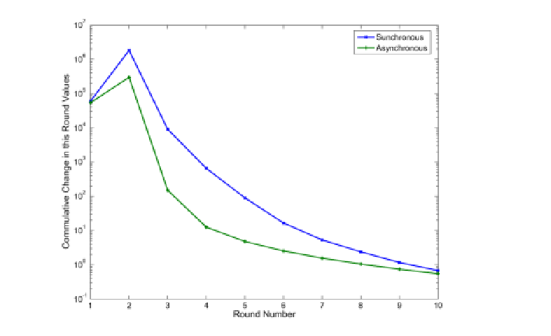
6.3.1 Rating Benchmark

For demonstrating the applicability of our proposed cost functions, we have chosen to implement a “benchmark” that evaluates the effectiveness of the various cost functions. Demonstrating this requires a quantitative measure beyond mere speed and scalability. The benchmark approach we take is as follows. First, we produce a ladder of “social influence” that is inferred from the network topology, and rank nodes by this ladder, using the Spatial ranking cost function. Next, we test our Peer-to-Peer rating method in the following settings. Some nodes are initialized with rate values, while other nodes are initialized with empty ratings. Influential nodes are given different initial ratings than non-influential nodes. The expected result is that the ratings of influential nodes should affect the ratings of the rest of the network so long as they are not vastly outnumbered by opposite ratings.

As a remark, we note that we can use the social ranks additionally as trust indicators, giving higher trust values to edges which are incident to high ranking nodes, and vice versa. This has the nice effect of initially placing low trust on intruders, which by assumption, cannot appear influential.

For performing our benchmark tests, we once again used simulation over the $1$ million nodes sub-graph of the Messenger network. Using the ranks produced by our spatial ranking, we selected the seven highest ranking nodes and assigned them an initial rating value $5$ . We also selected seven of the lowest ranking nodes and initialized them with rating value $1$ . All other nodes started with null input. The results of the rating system in this settings are given in Figure 3. After about ten rounds, a majority of the nodes converged to a rating very close to the one proposed by the influential nodes. We ran a variety of similar tests and obtained similar results in all cases where the influential nodes were not totally outnumbered by opposite initial ratings; for brevity, we report only one such test here.

The conclusion we draw from this test is that a combination of applying our GaBP solver for computing first the rating of nodes, and then using this rating for choosing influential nodes and spreading their beliefs in the network has the desired effect of fast and influential dissemination of the socially influential nodes. This effect can have a lot of applications in practice, including targeted commercials to certain zones in the social network.

Quite importantly, our experiment shows that our framework provide good protection against malicious infiltrators: Assuming that intruders have low connectivity to the rest of the network, we demonstrate that it is hard for them to influence the rating values in the system. Furthermore, we note that this property will be reinforced if the trust values on edges are reduced due to their low ranks, and using users satisfaction feedback.

Chapter 7 Linear Detection

Consider a discrete-time channel with a real input vector ${\bf x}=\{x_{1},\ldots,x_{K}\}^{T}$ and a corresponding real output vector ${\bf y}=\{y_{1},\ldots,y_{K}\}^{T}=f\{{\bf x}^{T}\}\in\mathbb{R}^{K}$ .¹¹ 1 An extension to the complex domain is straightforward. Here, the function $f\{\cdot\}$ denotes the channel transformation. Specifically, CDMA multiuser detection problem is characterized by the following linear channel

{\bf y}={\bf S}{\bf x}+{\bf n}\,,

where ${\bf S}_{N\times K}$ is the CDMA chip sequence matrix, ${\bf x}\in\{-1,1\}^{K}$ is the transmitted signal, ${\bf y}\in\mathbb{R}^{N}$ is the observation vector and ${\bf n}$ is a vector of AWGN noise. The multiuser detection problem is stated as follows. Given ${\bf S},{\bf y}$ and knowledge about the noise, we would like to infer the most probable ${\bf x}$ . This problem is NP-hard.

The matched filter output is

{\bf S}^{T}{\bf y}={\bf R}{\bf x}+{\bf S}^{T}{\bf n}\,,

where ${\bf S}^{T}{\bf n}$ is a $K\times 1$ additive noise vector and ${{\bf R}_{{\bf k}\times{\bf k}}}={\bf S}^{T}{\bf S}$ is a positive-definite symmetric matrix, often known as the correlation matrix.

Typically, the binary constraint on ${\bf x}$ is relaxed to ${\bf x}\in[-1,1]$ . This relaxation is called linear detection. In linear detection the decision rule is

\hat{{\bf x}}=\Delta\{{\bf x}^{\ast}\}=\Delta\{{\bf R}^{-1}{\bf S}^{T}{\bf y}\}\,.\

(7.1)

The vector ${\bf x}^{\ast}$ is the solution (over $\mathbb{R}$ ) to ${\bf R}{\bf x}={\bf S}^{T}{\bf y}$ . Estimation is completed by adjusting the (inverse) matrix-vector product to the input alphabet, accomplished by using a proper clipping function $\Delta\{\cdot\}$ (e.g. , for binary signaling $\Delta\{\cdot\}$ is the sign function).

Assuming linear channels with AWGN with variance $\sigma^{2}$ as the ambient noise, the linear minimum mean-square error (MMSE) detector can be described by using ${\bf R}+\sigma^{2}{\bf I}_{K}$ , known to be optimal when the input distribution $P_{{\bf x}}$ is Gaussian. In general, linear detection is suboptimal because of its deterministic underlying mechanism (i.e. , solving a given set of linear equations), in contrast to other estimation schemes, such as MAP or maximum likelihood, that emerge from an optimization criteria.

The essence of detection theory is to estimate a hidden input to a channel from empirically-observed outputs. An important class of practical sub-optimal detectors is based on linear detection. This class includes, for instance, the conventional single-user matched filter, the decorrelator (also, called the zero-forcing equalizer), the linear minimum mean-square error (LMMSE) detector, and many other detectors with widespread applicability [66, 67]. In general terms, given a probabilistic estimation problem, linear detection solves a deterministic system of linear equations derived from the original problem, thereby providing a sub-optimal, but often useful, estimate of the unknown input.

Applying the GaBP solver to linear detection, we establish a new and explicit link between BP and linear detection. This link strengthens the connection between message-passing inference and estimation theory, previously seen in the context of optimal maximum a-posteriori (MAP) detection [68, 69] and several sub-optimal nonlinear detection techniques [70] applied in the context of both dense and sparse [71, 72] graphical models.

In the following experimental study, we examine the implementation of a decorrelator detector in a noiseless synchronous CDMA system with binary signaling and spreading codes based upon Gold sequences of length $m=7$ .²² 2 In this case, as long as the system is not overloaded, i.e. the number of active users $n$ is not greater than the spreading code’s length $m$ , the decorrelator detector yields optimal detection decisions. Two system setups are simulated, corresponding to $n=3$ and $n=4$ users, resulting in the cross-correlation matrices

{\bf R}_{3}=\frac{1}{7}\left(\begin{array}[]{rrr}7&-1&3\\ -1&7&-5\\ 3&-5&7\\ \end{array}\right),

(7.2)

and

{\bf R}_{4}=\frac{1}{7}\left(\begin{array}[]{rrrr}7&-1&3&3\\ -1&7&3&-1\\ 3&3&7&-1\\ 3&-1&-1&7\\ \end{array}\right),

(7.3)

respectively.³³ 3 These particular correlation settings were taken from the simulation setup of Yener et al. [13].

The decorrelator detector, a member of the family of linear detectors, solves a system of linear equations, ${\bf R}{\bf x}={\bf S}^{T}{\bf y}$ , thus the vector of decorrelator decisions is determined by taking the signum of the vector ${\bf R}^{-1}{\bf S}^{T}{\bf y}$ . Note that ${\bf R}_{3}$ and ${\bf R}_{4}$ are not strictly diagonally dominant, but their spectral radius are less than unity, since $\rho(|{\bf I}_{3}-{\bf R}_{3}|)=0.9008<1$ and $\rho(|{\bf I}_{4}-{\bf R}_{4}|)=0.8747<1$ , respectively. In all of the experiments, we assumed the output vector was the all-ones vector.

Table 7.1 compares the proposed GaBP algorithm with standard iterative solution methods [2] (using random initial guesses), previously employed for CDMA multiuser detectors (MUD). Specifically, MUD algorithms based on the algorithms of Jacobi, Gauss-Seidel (GS) and (optimally weighted) successive over-relaxation (SOR)⁴⁴ 4 This moving average improvement of Jacobi and GS algorithms is equivalent to what is known in the BP literature as ‘damping’ [73]. were investigated [11, 12]. The table lists the convergence rates for the two Gold code-based CDMA settings. Convergence is identified and declared when the differences in all the iterated values are less than $10^{-6}$ . We see that, in comparison with the previously proposed detectors based upon the Jacobi and GS algorithms, the GaBP detectors converge more rapidly for both $n=3$ and $n=4$ . The serial (asynchronous) GaBP algorithm achieves the best overall convergence rate, surpassing even the SOR-based detector.

Algorithm Iterations $t$ ( ${\bf R}_{3}$ ) Iterations $t$ ( ${\bf R}_{4}$ ) Jacobi 111 24 GS 26 26 Parallel GaBP 23 24 Optimal SOR 17 14 Serial GaBP 16 13

Table 7.1: Decorrelator for

K=3,4

-user,

N=7

Gold code CDMA. Total number of iterations required for convergence (threshold

\epsilon=10^{-6}

) for GaBP-based solvers vs. standard methods.

Algorithm ${\bf R}_{3}$ ${\bf R}_{4}$ Jacobi+Steffensen⁵⁵footnotemark: 5 59 $-$ Parallel GaBP+Steffensen 13 13 Serial GaBP+Steffensen 9 7

Table 7.2: Decorrelator for

K=3,4

-user,

N=7

Gold code CDMA. Total number of iterations required for convergence (threshold

\epsilon=10^{-6}

) for Jacobi, parallel and serial GaBP solvers accelerated by Steffensen iterations.

Further speed-up of GaBP can be achieved by adapting known acceleration techniques from linear algebra, such Aitken’s method and Steffensen’s iterations, as explained in Section 3.2. Table 7.2 demonstrates the speed-up of GaBP obtained by using these acceleration methods, in comparison with that achieved by the similarly modified Jacobi algorithm.⁶⁶ 6 Application of Aitken and Steffensen’s methods for speeding-up the convergence of standard (non-BP) iterative solution algorithms in the context of MUD was introduced by Leibig et al. [74]. We remark that, although the convergence rate is improved with these enhanced algorithms, the region of convergence of the accelerated GaBP solver remains unchanged.

For the algorithms we examined, Figure 7.1.1 displays the Euclidean distance between the tentative (intermediate) results and the fixed-point solution as a function of the number of iterations. As expected, all linear algorithms exhibit a logarithmic convergence behavior. Note that GaBP converges faster on average, although there are some fluctuations in the GaBP curves, in contrast to the monotonicity of the other curves.

An interesting question concerns the origin of this convergence speed-up associated with GaBP. Better understanding may be gained by visualizing the iterations of the different methods for the matrix ${\bf R}_{3}$ case. The convergence contours are plotted in the space of $\{x_{1},x_{2},x_{3}\}$ in Fig. 7.3. As expected, the Jacobi algorithm converges in zigzags towards the fixed point (this behavior is well-explained in Bertsekas and Tsitsiklis [46]). The fastest algorithm is serial GaBP. It is interesting to note that GaBP convergence is in a spiral shape, hinting that despite the overall convergence improvement, performance improvement is not guaranteed in successive iteration rounds. In this case the system was simulated with a specific ${\bf R}$ matrix for which Jacobi algorithm and other standard methods did not even converge. Using Aitken’s method, a further speed-up in GaBP convergence was obtained.

Despite the fact that the examples considered correspond to small multi-user systems, we believe that the results reflect the typical behavior of the algorithms, and that similar qualitative results would be observed in larger systems. In support of this belief, we note, in passing, that GaBP was experimentally shown to converge in a logarithmic number of iterations in the cases of very large matrices both dense (with up to hundreds of thousands of dimensions [75]) and sparse (with up to millions of dimensions [20]).

As a final remark on the linear detection example, we mention that, in the case of a channel with Gaussian input signals, for which linear detection is optimal, the proposed GaBP scheme reduces to the BP-based MUD scheme, recently introduced by Montanari et al. [50], as shown in Chapter 11.1. Montanari’s BP scheme, assuming a Gaussian prior, has been proven to converge to the MMSE (and optimal) solution for any arbitrarily loaded, randomly-spread CDMA system (i.e. , a system where $\rho(|{\bf I}_{n}-{\bf R}|)\lesseqgtr 1$ ).⁷⁷ 7 For non-Gaussian signaling, e.g. with binary input alphabet, this BP-based detector is conjectured to converge only in the large-system limit, as $n,m\rightarrow\infty$ [50].Thus Gaussian-input additive white Gaussian noise CDMA is another example for which the proposed GaBP solver converges to the MAP decisions for any $m\times n$ random spreading matrix ${\bf S}$ , regardless of the spectral radius.

7.1 Extending GaBP to support non-square matrices

In the previous section, linear detection has been explicitly linked to BP [7], using a Gaussian belief propagation (GaBP) algorithm. This allows for an efficient iterative computation of the linear detector [14], circumventing the need of, potentially cumbersome, direct matrix inversion (via, e.g. , Gaussian elimination). The derived iterative framework was compared quantitatively with ‘classical’ iterative methods for solving systems of linear equations, such as those investigated in the context of linear implementation of CDMA demodulation [11, 12, 13]. GaBP is shown to yield faster convergence than these standard methods. Another important work is the BP-based MUD, recently derived and analyzed by Montanari et al. [50] for Gaussian input symbols.

There are several drawbacks to the linear detection technique presented earlier [7]. First, the input matrix ${\bf R}_{n\times n}={\bf S}_{n\times k}^{T}{\bf S}_{k\times n}$ (the chip correlation matrix) needs to be computed prior to running the algorithm. This computation requires $n^{2}k$ operations. In case where the matrix ${\bf S}$ is sparse [72], the matrix ${\bf R}$ might not no longer be sparse. Second, GaBP uses $2n^{2}$ memory to store the messages. For a large $n$ this could be prohibitive.

In this section, we propose a new construction that addresses those two drawbacks. In our improved construction, given a non-rectangular CDMA matrix ${\bf S}_{n\times k}$ , we compute the MMSE detector ${\bf x}=({\bf S}^{T}{\bf S}+\Psi)^{-1}{\bf S}^{T}y$ , where $\Psi=\sigma^{-2}{\bf I}$ is the AWGN diagonal inverse covariance matrix. We utilize the GaBP algorithm which is an efficient iterative distributed algorithm. The new construction uses only $2nk$ memory for storing the messages. When $k\ll n$ this represents significant saving relative to the $2n^{2}$ in our previously proposed algorithm. Furthermore, we do not explicitly compute ${\bf S}^{T}{\bf S}$ , saving an extra $n^{2}k$ overhead.

In Chapter 11.1 we show that Montanari’s algorithm [50] is an instance of GaBP. By showing this, we are able to prove new convergence results for Montanari’s algorithm. Montanari proves that his method converges on normalized random-spreading CDMA sequences, assuming Gaussian signaling. Using binary signaling, he conjectures convergence to the large system limit. Here, we extend Montanari’s result, to show that his algorithm converges also for non-random CDMA sequences when binary signaling is used, under weaker conditions. Another advantage of our work is that we allow different noise levels per bit transmitted.

7.1.1 Distributed Iterative Computation of the MMSE Detector

In this section, we efficiently extend the applicability of the proposed GaBP-based solver for systems with symmetric matrices [7] to systems with any square (i.e. , also nonsymmetric) or rectangular matrix. We first construct a new symmetric data matrix $\tilde{{\bf R}}$ based on an arbitrary (non-rectangular) matrix ${\bf S}\in\mathbb{R}^{k\times n}$

\tilde{{\bf R}}\triangleq\left(\begin{array}[]{cc}{\bf I}_{k}&{\bf S}^{T}\\ {\bf S}&-\Psi\\ \end{array}\right)\in\mathbb{R}^{(k+n)\times(k+n)}.

(7.4)

Additionally, we define a new vector of variables $\tilde{{\bf x}}\triangleq\{\hat{{\bf x}}^{T},{\bf z}^{T}\}^{T}\in\mathbb{R}^{(k+n)\times 1}$ , where $\hat{{\bf x}}\in\mathbb{R}^{k\times 1}$ is the (to be shown) solution vector and ${\bf z}\in\mathbb{R}^{n\times 1}$ is an auxiliary hidden vector, and a new observation vector $\tilde{{\bf y}}\triangleq\{\mathbf{0}^{T},{\bf y}^{T}\}^{T}\in\mathbb{R}^{(k+n)\times 1}$ .

Now, we would like to show that solving the symmetric linear system $\tilde{{\bf R}}\tilde{{\bf x}}=\tilde{{\bf y}}$ and taking the first $k$ entries of the corresponding solution vector $\tilde{{\bf x}}$ is equivalent to solving the original (not necessarily symmetric) system ${\bf R}{\bf x}={\bf y}$ . Note that in the new construction the matrix $\tilde{{\bf R}}$ is sparse again, and has only $2nk$ off-diagonal nonzero elements. When running the GaBP algorithm we have only $2nk$ messages, instead of $n^{2}$ in the previous construction.

Writing explicitly the symmetric linear system’s equations, we get

\hat{{\bf x}}+{\bf S}^{T}{\bf z}=\mathbf{0},\ \ \ \ {\bf S}\hat{{\bf x}}-\Psi{\bf z}={\bf y}.

Thus,

\hat{{\bf x}}=\Psi^{-1}{\bf S}^{T}({\bf y}-{\bf S}\hat{{\bf x}}),

and extracting $\hat{{\bf x}}$ we have

\hat{{\bf x}}=({\bf S}^{T}{\bf S}+\Psi)^{-1}{\bf S}^{T}{\bf y}.

Note, that when the noise level is zero, $\Psi=0_{m\times m}$ , we get the Moore-Penrose pseudoinverse solution

\hat{{\bf x}}=({\bf S}^{T}{\bf S})^{-1}{\bf S}^{T}{\bf y}={\bf S}^{{\dagger}}{\bf y}.

7.1.2 Relation to Factor Graph

In this section we give an alternate proof of the correctness of our construction. Given the inverse covariance matrix $\tilde{{\bf R}}$ defined in (7.4), and the shift vector $\tilde{{\bf x}}$ we can derive the matching self and edge potentials

\psi_{ij}(x_{i},x_{j})\triangleq\exp(-x_{i}R_{ij}x_{j})\,,

\phi_{i}(x_{i})\triangleq\exp(-1/2x_{i}R_{ii}^{2}x_{i}-x_{i}y_{i})\,,

which is a factorization of the Gaussian system distribution

p({\bf x})\propto\prod_{i}\phi_{i}(x_{i})\prod_{i,j}\psi_{ij}(x_{i},x_{j})=\prod_{i\leq k}\phi_{i}(x_{i})\prod_{i>k}\phi_{i}(x_{i})\prod_{i,j}\psi_{ij}(x_{i},x_{j})=

=\prod_{i\leq k}\overbrace{\exp(-\frac{1}{2}x_{i}^{2})}^{\mbox{ prior on x}}\prod_{i>k}\exp(-\frac{1}{2}\Psi_{i}x_{i}^{2}-x_{i}y_{i})\prod_{i,j}\exp(-x_{i}\overbrace{S_{ij}}^{R_{ij}}x_{j}).

Next, we show the relation of our construction to a factor graph. We will use a factor graph with $k$ nodes to the left (the bits transmitted) and $n$ nodes to the right (the signal received), shown in Fig 7.4. Using the definition $\tilde{{\bf x}}\triangleq\{\hat{{\bf x}}^{T},{\bf z}^{T}\}^{T}\in\mathbb{R}^{(k+n)\times 1}$ the vector $\hat{{\bf x}}$ represents the $k$ input bits and the vector ${\bf z}$ represents the signal received. Now we can write the system probability as:

p(\tilde{{\bf x}})\propto\int_{\hat{{\bf x}}}\mathcal{N}(\hat{{\bf x}};0,I)\mathcal{N}({\bf z};S\hat{{\bf x}},\Psi)d\hat{{\bf x}}\,.

It is known that the marginal distribution over ${\bf z}$ is:

=\mathcal{N}({\bf z};0,{\bf S}^{T}{\bf S}+\Psi).

The marginal distribution is Gaussian, with the following parameters:

E({\bf z}|\hat{{\bf x}})=({\bf S}^{T}{\bf S}+\Psi)^{-1}{\bf S}^{T}{\bf y},

Cov({\bf z}|\hat{{\bf x}})=({\bf S}^{T}{\bf S}+\Psi)^{-1}.

It is interesting to note that a similar construction was used by Frey [76] in his seminal 1999 work when discussing the factor analysis learning problem. Comparison to Frey’s work is found in Chapter 11.2.

7.1.3 Convergence Analysis

In this section we characterize the convergence properties of our linear detection method base on GaBP. We know that if the matrix $\tilde{{\bf R}}$ is strictly diagonally dominant, then GaBP converges and the marginal means converge to the true means [8, Claim 4]. Noting that the matrix $\tilde{{\bf R}}$ is symmetric, we can determine the applicability of this condition by examining its columns. As shown in Figure 7.5 we see that in the first $k$ columns, we have the $k$ CDMA sequences. We assume random-spreading binary CDMA sequences where the total system power is normalized to one. In other words, the absolute sum of each column is $1$ . By adding $\epsilon$ to the main diagonal, we insure that the first $k$ columns are diagonally dominant. In the next $n$ columns of the matrix $\tilde{{\bf R}}$ , we have the diagonal covariance matrix $\Psi$ with different noise levels per bit in the main diagonal, and zero elsewhere. The absolute sum of each column of $S$ is $k/n$ , thus when the noise level of each bit satisfies $\Psi_{i}>k/n$ , we have a convergence guarantee. Note, that the convergence condition is a sufficient condition. Based on Montanari’s work, we also know that in the large system limit, the algorithm converges for binary signaling, even in the absence of noise.

\left(\begin{array}[]{cccc|cccccc}1&0&\cdots&0&1/n&-1/n&-1/n&1/n&\ldots&1/n\\ 0&1&&0&&&&&&\\ \cdots&&\ddots&&&&&&&\\ 0&0&\cdots&1&1/n&-1/n&1/n&-1/n&\ldots&-1/n\\ \hline\cr 1/n&\cdots&&1/n&\Psi_{1}&0&0&&\cdots&0\\ -1/n&&&-1/n&0&\Psi_{2}&&&&\ldots\\ -1/n&&&1/n&&&&&&\\ 1/n&&&-1/n&&&&&&\\ \vdots&&&\vdots&&&&&\ddots&0\\ 1/n&&&-1/n&&&&\cdots&0&\Psi_{n}\\ \end{array}\right)

Figure 7.5: An example randomly spreading CDMA sequences matrices using our new construction. Using this illustration, it is easy to give a sufficient convergence proof to the GaBP algorithm. Namely, when the above matrix is diagonally dominant.

In Chapter 11.1 we prove that Montanari’s algorithm is an instance of our algorithm, thus our convergence results apply to Montanari’s algorithm as well.

7.2 Applying GaBP Convergence Fix

Next, we apply our novel double loop technique described in Chapter 5, for forcing the convergence of our linear detection algorithm using GaBP. We use the following setting: given a random-spreading CDMA code⁸⁸ 8 Randomly-spread CDMA code is a code where the matrix ${\bf S}$ is initialized uniformly with the entries $\pm\tfrac{1}{n}$ . with chip sequence length $n=256$ , and $k=64$ users. We assume a diagonal AWGN with $\sigma^{2}=1$ . Matlab code of our implementation is available on [77].

Using the above settings, we have drawn at random random-spreading CDMA matrix. Typically, the sufficient convergence conditions for the GaBP algorithm do not hold. For example, we have drawn at random a randomly-spread CDMA matrix with $\rho(|I_{K}-{C^{N}}|)=4.24$ , where $C^{N}$ is a diagonally-normalized version of $(C+\sigma^{2}I_{K})$ . Since $\rho(|I_{K}-{C^{N}}|)>1$ , the GaBP algorithm for multiuser detection is not guaranteed to converge.

Figure 7.6 shows that under the above settings, the GaBP algorithm indeed diverged. The $x$ -axis represent iteration number, while the values of different $x_{i}$ are plotted using different colors. This figure depicts well the fluctuating divergence behavior.

Next, we deployed our proposed construction and used a diagonal loading to force convergence. Figure 7.7 shows two different possible diagonal loadings. The $x$ -axis shows the Newton step number, while the $y$ -axis shows the residual. We experimented with two options of diagonal loading. In the first, we forced the matrix to be diagonally-dominant (DD). In this case, the spectral radius $\rho=0.188$ . In the second case, the matrix was not DD, but the spectral radius was $\rho=0.388$ . Clearly, the Newton method converges faster when the spectral radius is larger. In both cases the inner iterations converged in five steps to an accuracy of $10^{-6}$ .

The tradeoff between the amount of diagonal weighting to the total convergence speed is shown in Figures 3,4. A CDMA multiuser detection problem is shown ( $k=128$ , $n=256$ ). Convergence threshold for the inner and outer loops where $10^{-6}$ and $10^{-3}$ . The $x$ -axis present the amount of diagonal weighting normalized such that 1 is a diagonally-dominant matrix. $y$ -axis represent the number of iterations. As expected, the outer loop number of iterations until convergence grows with $\gamma$ . In contrast, the average number of inner loop iterations per Newton step (Figure 4) tends to decrease as $\gamma$ increases. The total number of iterations (inner $\times$ outer) represents the tradeoff between the inner and outer iterations and has a clear global minima.

Chapter 8 Support Vector Regression

In this chapter, we introduce a distributed support vector regression solver based on the Gaussian Belief Propagation (GaBP) algorithm. We improve on the original GaBP algorithm by reducing the communication load, as represented by the number of messages sent in each optimization iteration, from $n^{2}$ to $n$ aggregated messages, where $n$ is the number of data points. Previously, it was known that the GaBP algorithm is very efficient for sparse matrices. Using our novel construction, we demonstrate that the algorithm exhibits very good performance for dense matrices as well. We also show that the GaBP algorithm can be used with kernels, thus making the algorithm more powerful than previously possible.

Using extensive simulation we demonstrate the applicability of our protocol vs. the state-of-the-art existing parallel SVM solvers. Using a Linux cluster of up to a hundred machines and the IBM Blue Gene supercomputer we managed to solve very large data sets up to hundreds of thousands data point, using up to 1,024 CPUs working in parallel. Our comparison shows that the proposed algorithm is just as accurate as these solvers, while being significantly faster.

We start by giving on overview of the related SVM problem.

8.1 Classification Using Support Vector Machines

We begin by formulating the SVM problem. Consider a training set:

\begin{array}[]{l}D=\left\{\left(\mathbf{x}_{i},y_{i}\right),\;\;\;i=1,\ldots,N,\;\;\;\mathbf{x}_{i}\in\mathbb{R}^{m},\;\;\;y_{i}\in\left\{-1,1\right\}\right\}.\end{array}

(8.1)

The goal of the SVM is to learn a mapping from $\mathbf{x}_{i}$ to $y_{i}$ such that the error in mapping, as measured on a new dataset, would be minimal. SVMs learn to find the linear weight vector that separates the two classes so that

\begin{array}[]{l}y_{i}\left(\mathbf{x_{i}}\cdot\mathbf{w}+b\right)\geq 1\;\;for\;\;i=1,\ldots,N.\end{array}

(8.2)

There may exist many hyperplanes that achieve such separation, but SVMs find a weight vector $\mathbf{w}$ and a bias term $b$ that maximize the margin $2/\left\|\mathbf{w}\right\|$ . Therefore, the optimization problem that needs to be solved is

\min J_{D}(\mathbf{w})=\frac{1}{2}\left\|\mathbf{w}\right\|,

(8.3)

\mbox{subject to \;}y_{i}\left(\mathbf{x_{i}}\cdot\mathbf{w}+b\right)\geq 1\;\;for\;\;i=1,\ldots,N.

(8.4)

Points lying on the hyperplane $y_{i}\left(\mathbf{x_{i}}\cdot\mathbf{w}+b\right)=1$ are called support vectors.

If the data cannot be separated using a linear separator, a slack variable $\xi\geq 0$ is introduced and the constraint is relaxed to:

y_{i}\left(\mathbf{x_{i}}\cdot\mathbf{w}+b\right)\geq 1-\xi_{i}\;\;for\;\;i=1,\ldots,N.

(8.5)

The optimization problem then becomes:

\min J_{D}(\mathbf{w})=\tfrac{1}{2}\left\|\mathbf{w}\right\|^{2}_{2}+C\sum_{i=1}^{N}\xi_{i},

(8.6)

\mbox{subject to \;}y_{i}\left(\mathbf{x_{i}}\cdot\mathbf{w}+b\right)\geq 1\;\;for\;\;i=1,\ldots,N,\newline

(8.7)

\xi_{i}\geq 0\;\;for\;\;i=1,\ldots,N.

(8.8)

The weights of the linear function can be found directly or by converting the problem into its dual optimization problem, which is usually easier to solve.

Using the notation of Vijayakumar and Wu [78], the dual problem is thus:

\max\;\;L_{D}(h)=\sum_{i}h_{i}-\tfrac{1}{2}h^{T}Dh\,,\\

(8.9)

\mbox{subject \; to \;\;}0\leq h_{i}\leq C,\;\;i=1,...,N\,,\\

(8.10)

\;\;\;\;\;\;\;\;\Sigma_{i}h_{i}y_{i}=0\,,

(8.11)

where $D$ is a matrix such that $D_{ij}=y_{i}y_{j}K\left(\mathbf{x}_{i},\mathbf{x}_{j}\right)$ and $K\left(\cdot,\;\cdot\right)$ is either an inner product of the samples or a function of these samples. In the latter case, this function is known as the kernel function, which can be any function that complies with the Mercer conditions [79]. For example, these may be polynomial functions, radial-basis (Gaussian) functions, or hyperbolic tangents. If the data is not separable, $C$ is a tradeoff between maximizing the margin and reducing the number of misclassifications.

The classification of a new data point is then computed using the following equation:

f\left(x\right)=\mathop{sign}\left(\sum_{i\in SV}h_{i}y_{i}K\left(x_{i},x\right)+b\right)

(8.12)

8.2 Kernel Ridge Regression problem

Kernel Ridge Regression (KRR) implements a regularized form of the least squares method useful for both regression and classification. The non-linear version of KRR is similar to Support-Vector Machine (SVM) problem. However, in the latter, special emphasis is given to points close to the decision boundary, which is not provided by the cost function used by KRR.

Given training data

\mathcal{D}=\{{\bf x}_{i},y_{i}\}_{i=1}^{l},\mbox{ }{\bf x}_{i}\in R^{d}\mbox{ },y_{i}\in R\,,

the KRR algorithm determines the parameter vector ${\bf w}\in R^{d}$ of a non-linear model (using the “kernel trick”), via minimization of the following objective function: [75]:

\min\lambda||{\bf w}||^{2}+\sum_{i=1}^{l}(y_{i}-{\bf w}^{T}\Phi({\bf x}_{i}))^{2}\,,

where $\lambda$ is a tradeoff parameter between the two terms of the optimization function, and $\Phi(\dot{)}$ is a (possible non-linear) mapping of the training patterns.

One can show that the dual form of this optimization problem is given by:

\max W(\alpha)={\bf y}^{T}\alpha+\tfrac{1}{4}\lambda\alpha^{T}{\bf K}\alpha-\tfrac{1}{4}\alpha^{T}\alpha\,,

(8.13)

where ${\bf K}$ is a matrix whose $(i,j)$ -th entry is the kernel function ${\bf K}_{i,j}=\Phi({\bf x}_{i})^{T}\Phi({\bf x}_{j})$ .

The optimal solution to this optimization problem is:

\alpha=2\lambda({\bf K}+\lambda{\bf I})^{-1}{\bf y}

The corresponding prediction function is given by:

f({\bf x})={\bf w}^{T}\Phi({\bf x})={\bf y}^{T}({\bf K}+\lambda{\bf I})^{-1}{\bf K}({\bf x}_{i},{\bf x}).

8.3 Previous Approaches for Solving Parallel SVMs

There are several main methods for finding a solution to an SVM problem on a single-node computer. (See [79, Chapter 10]) for a taxonomy of such methods.) However, since solving an SVM is quadratic in time and cubic in memory, these methods encounter difficulty when scaling to datasets that have many examples and support vectors. The latter two are not synonymous. A large dataset with many repeated examples might be solved using sub-sampling approaches, while a highly non-separable dataset with many support vectors will require an altogether different solution strategy. The literature covers several attempts at solving SVMs in parallel, which allow for greater computational power and larger memory size. In Collobert et al. [80] the SVM solver is parallelized by training multiple SVMs, each on a subset of the training data, and aggregating the resulting classifiers into a single classifier. The training data is then redistributed to the classifiers according to their performance and the process is iterated until convergence is reached. The need to re-divide the data among the SVM classifiers implies that the data must be exchanged between nodes several times; this rules out the use of an approach where bandwidth is a concern. A more low-level approach is taken by Zanghirati et al. [81], where the quadratic optimization problem is divided into smaller quadratic programs, each of which is solved on a different node. The results are aggregated and the process is repeated until convergence. The performance of this method has a strong dependence on the caching architecture of the cluster. Graf et al. [82] partition the data and solve an SVM for each partition. The support vectors from each pair of classifiers are then aggregated into a new training set for which an SVM is solved. The process continues until a single classifier remains. The aggregation process can be iterated, using the support vectors of the final classifier in the previous iteration to seed the new classifiers. One problem with this approach is that the data must be repeatedly shared between nodes, meaning that once again the goal of data distribution cannot be attained. The second problem, which might be more severe, is that the number of possible support vectors is restricted by the capacity of a single SVM solver. Yom Tov [83] proposed modifying the sequential algorithm developed in [78] to batch mode. In this way, the complete kernel matrix is held in distributed memory and the Lagrange multipliers are computed iteratively. This method has the advantage that it can efficiently solve difficult SVM problems that have many support vectors to their solution. Based on that work, we show how an SVM solution can be obtained by adapting a Gaussian Belief Propagation algorithm to the solution of the algorithm proposed in [78].

Recently, Hazan et al. proposed an iterative algorithm for parallel decomposition based on Fenchel Duality [84]. Zanni et al. propose a decomposition method for computing SVM in parallel [85]. We compare our running time results to both systems in Section 8.5.

For our proposed solution, we take the exponent of dual SVM formulation given in equation (8.9) and solve $\max\exp(L_{D}(h))$ . Since $\exp(L_{D}(h))$ is convex, the solution of $\max\exp(L_{D}(h))$ is a global maximum that also satisfies $\max L_{D}(h)$ since the matrix $D$ is symmetric and positive definite. Now we can relate to the new problem formulation as a probability density function, which is in itself Gaussian:

p(h)\propto\exp(-\tfrac{1}{2}h^{T}Dh+h^{T}\mathbf{1}),

where $\mathbf{1}$ is a vector of $(1,1,\cdots,1),$ and find the assignment of $\hat{h}=\arg\max p(h)$ . To solve the inference problem, namely computing the marginals $\hat{h}$ , we propose using the GaBP algorithm, which is a distributed message passing algorithm. We take the computed $\hat{h}$ as the Lagrange multiplier weights of the support vectors of the original SVM data points and apply a threshold for choosing data points with non-zero weight as support vectors.

Note that using this formulation we ignore the remaining constraints (8.10), (8.11). In other words we do not solve the SVM problem, but the unconstrained kernel ridge regression problem (8.13). Nevertheless, empirical results presented in Chapter 8.5 show that we achieve a very good classification vs. state-of-the-art SVM solvers.

Finally, following [78], we remove the explicit bias term $b$ and instead add another dimension to the pattern vector $\mathbf{x}_{i}$ such that $\mathbf{\hat{x_{i}}}=\left(x_{1},x_{2},\ldots,x_{N},\lambda\right)$ , where $\lambda$ is a scalar constant. The modified weight vector, which incorporates the bias term, is written as $\mathbf{\hat{w}}=\left(w_{1},w_{2},\ldots,w_{N},b/\lambda\right)$ . However, this modification causes a change to the optimized margin. Vijayakumar and Wu [78] discuss the effect of this modification and reach the conclusion that “setting the augmenting term to zero (equivalent to neglecting the bias term) in high dimensional kernels gives satisfactory results on real world data”. We did not completely neglect the bias term and in our experiments, which used the Radial Basis Kernel, we set it to $1/N$ , as proposed in [83].

8.4 Our novel construction

We propose to use the GaBP algorithm for solving the SVR problem (8.13). In order to force the algorithm to converge, we artificially weight the main diagonal of the kernel matrix $D$ to make it diagonally dominant. Section 8.5 outlines our empirical results showing that this modification did not significantly affect the error in classifications on all tested data sets.

A partial justification for weighting the main diagonal is found in [75]. In the 2-Norm soft margin formulation of the SVM problem, the sum of squared slack variables is minimized:

\min_{\xi,w,b}\|\mathbf{w}\|_{2}^{2}+C\Sigma_{i}\mathbf{\xi}_{i}^{2}

\mbox{such that \ \ \ }y_{i}(\mathbf{w}\cdot\mathbf{x}_{i}+b)\geq 1-\xi_{i}

The dual problem is derived:

W(h)=\Sigma_{i}h_{i}-\frac{1}{2}\Sigma_{i,j}y_{i}y_{j}h_{i}h_{j}(\mathbf{x}_{i}\cdot\mathbf{x}_{j}+\tfrac{1}{C}\delta_{ij}),

where $\delta_{ij}$ is the Kronecker $\delta$ defined to be 1 when $i=j$ , and zero elsewhere. It is shown that the only change relative to the 1-Norm soft margin SVM is the addition of $1/C$ to the diagonal of the inner product matrix associated with the training set. This has the effect of adding $1/C$ to the eigenvalues, rendering the kernel matrix (and thus the GaBP problem) better conditioned [75].

One of the desired properties of a large scale algorithm is that it should converge in asynchronous settings as well as in synchronous settings. This is because in a large-scale communication network, clocks are not synchronized accurately and some nodes may be slower than others, while some nodes experience longer communication delays.

Corollary 25.

Assuming one of the convergence conditions (Theorems 14, 15) holds, the GaBP algorithm convergence using serial (asynchronous) scheduling as well.

Proof.

The quadratic Min-Sum algorithm [6] provides a convergence proof in the asynchronous case. In Chapter 11.4 we show equivalence of both algorithms. Thus, assuming one of the convergence conditions holds, the GaBP algorithm converges using serial scheduling as well. ∎

8.5 Experimental Results

We implemented our proposed algorithm using approximately 1,000 lines of code in C. We implemented communication between the nodes using the MPICH2 message passing interface.¹¹ 1 http://www-unix.mcs.anl.gov/mpi/mpich/ Each node was responsible for $d$ data points out of the total $n$ data points in the dataset.

Our implementation used synchronous communication rounds because of MPI limitations. In Section 8.6 we further elaborate on this issue.

Each node was assigned several examples from the input file. Then, the kernel matrix $D$ was computed by the nodes in a distributed fashion, so that each node computed the rows of the kernel matrix related to its assigned data points. After computing the relevant parts of the matrix $D$ , the nodes weighted the diagonal of the matrix $D$ , as discussed in Section 8.4. Then, several rounds of communication between the nodes were executed. In each round, using our optimization, a total of $n$ sums were calculated using MPI_Allreduce system call. Finally, each node output the solution $x$ , which was the mean of the input Gaussian that matched its own data points. Each $x_{i}$ signified the weight of the data point $i$ for being chosen as a support vector.

To compare our algorithm performance, we used two algorithms: Sequential SVM (SVMSeq) [78] and SVMlight [86]. We used the SVMSeq implementation provided within the IBM Parallel Machine Learning (PML) toolbox [87]. The PML implements the same algorithm by Vijaykumar and Wu [78] that our GaBP solver is based on, but the implementation in through a master-slave architecture as described in [83]. SVMlight is a single computing node solver.

Dataset	Dimension	Train	Test	Error (%)
				GaBP	Sequential	SVMlight
Isolet	617	6238	1559	7.06	5.84	49.97
Letter	16	20000		2.06	2.06	2.3
Mushroom	117	8124		0.04	0.05	0.02
Nursery	25	12960		4.16	5.29	0.02
Pageblocks	10	5473		3.86	4.08	2.74
Pen digits	16	7494	3498	1.66	1.37	1.57
Spambase	57	4601		16.3	16.5	6.57

Table 8.1: Error rates of the GaBP solver versus those of the parallel sequential solver and SVMlight.

Dataset	Run times (sec)
	GaBP	Sequential
Isolet	228	1328
Letter	468	601
Mushroom	226	176
Nursery	221	297
Pageblocks	26	37
Pen digits	45	155
Spambase	49	79

Table 8.2: Running times (in seconds) of the GaBP solver (working in a distributed environment) compared to that of the IBM parallel solver.

Table 8.1 describes the seven datasets we used to compare the algorithms and the classification accuracy obtained. These computations were done using five processing nodes (3.5GHz Intel Pentium machines, running the Linux operating system) for each of the parallel solvers. All datasets were taken from the UCI repository [88]. We used medium-sized datasets so that run-times using SVMlight would not be prohibitively high. All algorithms were run with an RBF kernel. The parameters of the algorithm (kernel width and misclassification cost) were optimized using a line-search algorithm, as detailed in [89].

Note that SVMlight is a single node solver, which we use mainly as a comparison for the accuracy in classification.

Using the Friedman test [90], we did not detect any statistically significant difference between the performance of the algorithms with regards to accuracy ( $p<0.10^{-3}$ ).

Figure 8.1 shows the speedup results of the algorithm when running the GaBP algorithm on a Blue Gene supercomputer. The speedup with $N$ nodes is computed as the run time of the algorithm on a single node, divided by the run time using $N$ nodes. Obviously, it is desirable to obtain linear speedup, i.e., doubling computational power halves the processing time, but this is limited by the communication load and by parts of the algorithm that cannot be parallelized. Since Blue Gene is currently limited to 0.5 GB of memory at each node, most datasets could not be executed on a single node. We therefore show speedup compared to two nodes. As the figure shows, in most cases we get a linear speedup up to 256 CPUs, which means that the running time is linearly proportional to one over the number of used CPUs. When using 512 - 1024 CPUs, the communication overhead reduces the efficiency of the parallel computation. We identified this problem as an area for future research into optimizing the performance for larger scale grids.

We also tested the ability to build classifiers for larger datasets. Table 8.3 shows the run times of the GaBP algorithm using 1024 CPUs on two larger datasets, both from the UCI repository. This demonstrates the ability of the algorithm to process very large datasets in a reasonably short amount of time. We compare our running time to state-of-the-art parallel decomposition method by Zanni et al. [85] and Hazan et al. . Using the MNIST dataset we where considerably slower by a factor of two, but in the larger Covertype dataset we have a superior performance. Note that the reported running times should be taken with a grain of salt, since the machines used for experimentation are different. Zanni used 16 Pentium IV machines with 16Gb memory, Hazan used 10 Pentium IV machines with 4Gb memory, while we used a larger number of weaker Pentium III machines with 400Mb of memory. Furthermore, in the Covertype dataset we used only 150,000 data points while Zanni and Hazan used the full dataset which is twice larger.

Dataset	Dim	Num of examples	Run time GaBP (sec)	Run time [85] (sec)	Run time [84]
Covertype	54	150,000/300,000	468	24365	16742
MNIST	784	60,000	756	359	18

Table 8.3: Running times of the GaBP solver for large data sets using 1024 CPUs on an IBM Blue Gene supercomputer. Running time results are compared to two state-of-the-art solvers: [85] and [84].

8.6 Discussion

In this chapter we demonstrated the application of the Gaussian Belief Propagation to the solution of SVM problems. Our experiments demonstrate the usefulness of this solver, being both accurate and scalable.

We implemented our algorithm using a synchronous communication model mainly because MPICH2 does not support asynchronous communication. While synchronous communication is the mode of choice for supercomputers such as Blue Gene, in many cases such as heterogeneous grid environments, asynchronous communication will be preferred. We believe that the next challenging goal will be to implement the proposed algorithm in asynchronous settings, where algorithm rounds will no longer be synchronized.

Our initial experiments with very large sparse kernel matrices (millions of data points) show that asynchronous settings converge faster. Recent work by Elidan et al. [65] supports this claim by showing that in many cases the BP algorithm converges faster in asynchronous settings.

Another challenging task would involve scaling to data sets of millions of data points. Currently the full kernel matrix is computed by the nodes. While this is effective for problems with many support vectors [83], it is not required in many problems that are either easily separable or where the classification error is less important compared to the time required to learn the mode. Thus, solvers scaling to much larger datasets may have to diverge from the current strategy of computing the full kernel matrix and instead sparsify the kernel matrix as is commonly done in single node solvers.

Finally, it remains an open question whether SVMs can be solved efficiently in Peer-to-Peer environments, where each node can (efficiently) obtain data from only several close peers. Future work will be required in order to verify how the GaBP algorithm performs in such an environment, where only partial segments of the kernel matrix can be computed by each node.

Chapter 9 Distributed Computation of Kalman Filter

In Chapter 7 we show how to compute efficiently and distributively the MMSE prediction for the multiuser detection problem, using the Gaussian Belief Propagation (GaBP) algorithm. The basic idea is to shift the problem from the linear algebra domain into a probabilistic graphical model, solving an equivalent inference problem using the efficient belief propagation inference engine.

In this chapter, we propose to extend the previous construction, and show, that by performing the MMSE computation twice on the matching inputs we are able to compute several algorithms: Kalman filter, Gaussian information bottleneck and the Affine-scaling interior point method. We reduce the discrete Kalman filter computation [91] to a matrix inversion problem and show how to solve it using the GaBP algorithm. We show that Kalman filter iteration that is composed from prediction and measurement steps can be computed by two consecutive MMSE predictions. We explore the relation to Gaussian information bottleneck (GIB) [92] and show that Kalman filter is a special instance of the GIB algorithm, when the weight parameter $\beta=1$ . To the best of our knowledge, this is the first algorithmic link between the information bottleneck framework and linear dynamical systems. We discuss the connection to the Affine-scaling interior-point method and show it is an instance of the Kalman filter.

Besides of the theoretical interest of linking compression, estimation and optimization together, our work is highly practical, since it proposes a general framework for computing all of the above tasks distributively in a computer network. This result can have many applications in the fields of estimation, collaborative signal processing, distributed resource allocation, etc.

A closely related work is [39]. In this work, Frey et al. focus on the belief propagation algorithm (a.k.a sum-product algorithm) using factor graph topologies. They show that the Kalman filter algorithm can be computed using belief propagation over a factor graph. In this contribution we extend their work in several directions. First, we extend the computation to vector variables (relative to scalar variables in Frey’s work). Second, we use a different graphical model: an undirected graphical model, which results in simpler update rules, where Frey uses factor-graph with two types of messages: factor to variables and variables to factors. Third and most important, we allow an efficient distributed calculation of the Kalman filter steps, where Frey’s algorithm is centralized.

Another related work is [93]. In this work the link between Kalman filter and linear programming is established. In this thesis we propose a new and different construction that ties the two algorithms.

9.1 Kalman Filter

The Kalman filter is an efficient iterative algorithm to estimate the state of a discrete-time controlled process $x\in R^{n}$ that is governed by the linear stochastic difference equation¹¹ 1 We assume there is no external input, namely $x_{k}=Ax_{k-1}+w_{k-1}$ . However, our approach can be easily extended to support external inputs.:

x_{k}=Ax_{k-1}+Bu_{k-1}+w_{k-1}\,,

(9.1)

with a measurement $z\in R^{m}$ that is $z_{k}=Hx_{k}+v_{k}.$ The random variables $w_{k}$ and $v_{k}$ that represent the process and measurement AWGN noise (respectively). $p(w)\sim\mathcal{N}(0,Q),p(v)\sim\mathcal{N}(0,R)$ . We further assume that the matrices $A,H,B,Q,R$ are given.²² 2 Another possible extension is that the matrices $A,H,B,Q,R$ change in time, in this thesis we assume they are fixed. However, our approach can be generalized to this case as well.

The discrete Kalman filter update equations are given by [91]:

The prediction step:


$\displaystyle\hat{x}^{-}_{k}$	$\displaystyle=$	$\displaystyle A\hat{x}_{k-1}+Bu_{k-1},$	(9.2a)
$\displaystyle P_{k}^{-}$	$\displaystyle=$	$\displaystyle AP_{k-1}A^{T}+Q.$	(9.2b)

The measurement step:


$\displaystyle K_{k}$	$\displaystyle=$	$\displaystyle P_{k}^{-}H^{T}(HP_{k}^{-}H^{T}+R)^{-1},$	(9.3a)
$\displaystyle\hat{x}_{k}$	$\displaystyle=$	$\displaystyle\hat{x}^{-}_{k}+K_{k}(z_{k}-H\hat{x}^{-}_{k}),$	(9.3b)
$\displaystyle P_{k}$	$\displaystyle=$	$\displaystyle(I-K_{k}H)P_{k}^{-}.$	(9.3c)

where $I$ is the identity matrix.

The algorithm operates in rounds. In round $k$ the estimates $K_{k},\hat{x}_{k},P_{k}$ are computed, incorporating the (noisy) measurement $z_{k}$ obtained in this round. The output of the algorithm are the mean vector $\hat{x}_{k}$ and the covariance matrix $P_{k}$ .

9.2 Our Construction

Our novel contribution is a new efficient distributed algorithm for computing the Kalman filter. We begin by showing that the Kalman filter can be computed by inverting the following covariance matrix:

E=\left(\begin{array}[]{ccc}-P_{k-1}&A&0\\ A^{T}&Q&H\\ 0&H^{T}&R\\ \end{array}\right)\,,

(9.4)

and taking the lower right $1\times 1$ block to be $P_{k}$ .

The computation of $E^{-1}$ can be done efficiently using recent advances in the field of Gaussian belief propagation [14, 19]. The intuition for our approach, is that the Kalman filter is composed of two steps. In the prediction step, given $x_{k}$ , we compute the MMSE prediction of $x_{k}^{-}$ [39]. In the measurement step, we compute the MMSE prediction of $x_{k+1}$ given $x_{k}^{-}$ , the output of the prediction step. Each MMSE computation can be done using the GaBP algorithm [19]. The basic idea is that given the joint Gaussian distribution $p({\bf x},{\bf y})$ with the covariance matrix $C=\left(\begin{array}[]{cc}\Sigma_{xx}&\Sigma_{xy}\\ \Sigma_{yx}&\Sigma_{yy}\\ \end{array}\right)$ , we can compute the MMSE prediction

\hat{y}=\argmax_{y}p(y|x)\propto\mathcal{N}(\mu_{y|x},\Sigma_{y|x}^{-1})\,,

where

\mu_{y|x}=(\Sigma_{yy}-\Sigma_{yx}\Sigma_{xx}^{-1}\Sigma_{xy})^{-1}\Sigma_{yx}\Sigma_{xx}^{-1}x\,,

\Sigma_{y|x}=(\Sigma_{yy}-\Sigma_{yx}\Sigma_{xx}^{-1}\Sigma_{xy})^{-1}\,.

This in turn is equivalent to computing the Schur complement of the lower right block of the matrix $C$ . In total, computing the MMSE prediction in Gaussian graphical model boils down to a computation of a matrix inverse. In [14] we have shown that GaBP is an efficient iterative algorithm for solving a system of linear equations (or equivalently computing a matrix inverse). In [19] we have shown that for the specific case of linear detection we can compute the MMSE estimator using the GaBP algorithm. Next, we show that performing two consecutive computations of the MMSE are equivalent to one iteration of the Kalman filter.

Theorem 26.

The lower right $1\times 1$ block of the matrix inverse $E^{-1}$ (eq. 9.4), computed by two MMSE iterations, is equivalent to the computation of $P_{k}$ done by one iteration of the Kalman filter algorithm.

Proof.

We prove that inverting the matrix $E$ (eq. 9.4) is equivalent to one iteration of the Kalman filter for computing $P_{k}$ .

We start from the matrix $E$ and show that $P_{k}^{-}$ can be computed in recursion using the Schur complement formula:

D-CA^{-1}B

(9.5)

applied to the $2\times 2$ upper left submatrix of E, where $D\triangleq Q,C\triangleq A^{T},B\triangleq A,A\triangleq P_{k-1}$ , we get:

P_{k}^{-}=\overbrace{Q}^{D}\overbrace{+}^{-}\overbrace{A^{T}}^{C}\overbrace{P_{k-1}}^{-A^{-1}}\overbrace{A}^{B}.

Now we compute recursively the Schur complement of lower right $2\times 2$ submatrix of the matrix $E$ using the matrix inversion lemma:

A^{-1}+A^{-1}B(D-CA^{-1}B)^{-1}CA^{-1}

where $A^{-1}\triangleq P_{k}^{-},B\triangleq H^{T},C\triangleq H,D\triangleq Q.$ In total we get:

\overbrace{P_{k}^{-}}^{A^{-1}}+\overbrace{P_{k}^{-}}^{A^{-1}}\overbrace{H^{T}}^{B}(\overbrace{R}^{D}+\overbrace{H}^{C}\overbrace{P_{k}^{-}}^{A^{-1}}\overbrace{H^{T}}^{B})^{-1}\overbrace{H}^{C}\overbrace{P_{k}^{-}}^{A^{-1}}=

(9.6)

(I-\overbrace{P_{k}^{-}H^{T}(HP_{k}^{-}H^{T}+R)^{-1}}^{(\ref{kalman_gain})}H)P_{k}^{-}=\overbrace{(I-K_{k}H)P_{k}^{-}}^{(\ref{p_k})}=P_{k}

∎

In Section 9.2 we explain how to utilize the above observation to an efficient distributed iterative algorithm for computing the Kalman filter.

9.3 Gaussian Information Bottleneck

Given the joint distribution of a source variable X and another relevance variable Y, Information bottleneck (IB) operates to compress X, while preserving information about Y [94, 95], using the following variational problem:

\min_{p(t|x)}\mathcal{L}:\mathcal{L}\equiv I(X;T)-\beta I(T;Y)

$T$ represents the compressed representation of $X$ via the conditional distributions $p(t|x)$ , while the information that $T$ maintains on $Y$ is captured by the distribution $p(y|t)$ . $\beta>0$ is a lagrange multiplier that weights the tradeoff between minimizing the compression information and maximizing the relevant information. As $\beta\rightarrow 0$ we are interested solely in compression, but all relevant information about Y is lost $I(Y;T)=0$ . When $\beta\rightarrow\infty$ we are focused on preservation of relevant information, in this case T is simply the distribution X and we obtain $I(T;Y)=I(X;Y)$ . The interesting cases are in between, when for finite values of $\beta$ we are able to extract rather compressed representation of X while still maintaining a significant fraction of the original information about Y.

An iterative algorithm for solving the IB problem is given in [95]:


$\displaystyle P^{k+1}(t\|x)=$	$\displaystyle\frac{P^{k}(t)}{Z^{k+1}(x,\beta)}\exp(-\beta D_{KL}[p(y\|x)\|\|p^{k}(y\|t)])\,,$
$\displaystyle P^{k}(t)=$	$\displaystyle\int_{x}p(x)P^{k}(t\|x)dx\,,$	(9.7a)
$\displaystyle P^{k}(y\|t)=$	$\displaystyle\frac{1}{P^{k}(t)}\int_{x}P^{k}(t\|x)p(x,y)dx\,\,,$	(9.7b)

where $Z^{k+1}$ is a normalization factor computed in round $k+1$ .

The Gaussian information bottleneck (GIB) [92] deals with the special case where the underlying distributions are Gaussian. In this case, the computed distribution $p(t)$ is Gaussian as well, represented by a linear transformation $T_{k}=A_{k}X+\xi_{k}$ where $A_{k}$ is a joint covariance matrix of $X$ and $T$ , $\xi_{k}\sim\mathcal{N}(0,\Sigma_{\xi_{k}})$ is a multivariate Gaussian independent of X. The outputs of the algorithm are the covariance matrices representing the linear transformation T: $A_{k},\Sigma_{\xi_{k}}$ .

An iterative algorithm is derived by substituting Gaussian distributions into (9.7), resulting in the following update rules:


$\displaystyle\Sigma_{\xi+1}$	$\displaystyle=$	$\displaystyle(\beta\Sigma_{t_{k}\|y}-(\beta-1)\Sigma_{t_{k}}^{-1}),$	(9.8a)
$\displaystyle A_{k+1}$	$\displaystyle=$	$\displaystyle\beta\Sigma_{\xi_{k}+1}\Sigma^{-1}_{t_{k}\|y}A_{k}(I-\Sigma_{y\|x}\Sigma_{x}^{-1}).$	(9.8b)

Table 9.1: Summary of notations in the GIB [92] paper vs. Kalman filter [91]

GIB [92]	Kalman [91]	Kalman meaning
$\Sigma_{x}$	$P_{0}$	a-priori estimate error covariance
$\Sigma_{y}$	$Q$	process AWGN noise
$\Sigma_{t_{k}}$	$R$	measurement AWGN noise
$\Sigma_{xy}$	$A$	process state transformation matrix
$\Sigma_{yx}$	$A^{T}$	-”-
$\Sigma_{xy}A$	$H^{T}$	measurement transformation matrix
$A^{T}\Sigma_{yx}$	$H$	-”-
$\Sigma_{\xi_{k}}$	$P_{k}$	posterior error covariance in round k
$\Sigma_{x\|y_{k}}$	$P_{k}^{-}$	a-priori error covariance in round k

Since the underlying graphical model of both algorithms (GIB and Kalman filter) is Markovian with Gaussian probabilities, it is interesting to ask what is the relation between them. In this work we show, that the Kalman filter posterior error covariance computation is a special case of the GIB algorithm when $\beta=1$ . Furthermore, we show how to compute GIB using the Kalman filter when $\beta>1$ (the case where $0<\beta<1$ is not interesting since it gives a degenerate solution where $A_{k}\equiv 0$ [92].) Table 9.1 outlines the different notations used by both algorithms.

Theorem 27.

The GIB algorithm when $\beta=1$ is equivalent to the Kalman filter algorithm.

Proof.

Looking at [92, $\lx@sectionsign 39$ ], when $\beta=1$ we get

\begin{array}[]{l}\Sigma_{\xi+1}=(\Sigma_{t_{k}|y}^{-1})^{-1}=\Sigma_{t_{k}|y}=\overbrace{\Sigma_{t_{k}}-\Sigma_{t_{k}y}\Sigma_{y}^{-1}\Sigma_{yt_{k}}}^{\mbox{MMSE}}=\overbrace{\Sigma_{t_{k}}+B^{T}\Sigma_{y|t_{k}}B}^{\mbox{\cite[cite]{[\@@bibref{}{GIB}{}{}, \lx@sectionsign 38b]}}}=\\ \Sigma_{t_{k}}+\overbrace{\Sigma_{t_{k}}^{-1}\Sigma_{t_{k}y}}^{\mbox{\cite[cite]{[\@@bibref{}{GIB}{}{}, \lx@sectionsign 34]}}}\Sigma_{y|t_{k}}\overbrace{\Sigma_{yt_{k}}\Sigma_{t_{k}}^{-1}}^{\mbox{\cite[cite]{[\@@bibref{}{GIB}{}{}, \lx@sectionsign 34]}}}=\overbrace{A^{T}\Sigma_{x}A+\Sigma_{\xi}}^{\mbox{\cite[cite]{[\@@bibref{}{GIB}{}{}, \lx@sectionsign 33]}}}+\overbrace{(A^{T}\Sigma_{x}A+\Sigma_{\xi})}^{\mbox{\cite[cite]{[\@@bibref{}{GIB}{}{}, \lx@sectionsign 33]}}}A^{T}\Sigma_{xy}\cdot\\ \cdot\Sigma_{y|t_{k}}\Sigma_{yx}A\overbrace{(A^{T}\Sigma_{x}A+\Sigma_{\xi})^{T}}^{\mbox{\cite[cite]{[\@@bibref{}{GIB}{}{}, \lx@sectionsign 33]}}}=A^{T}\Sigma_{x}A+\Sigma_{\xi}+(A^{T}\Sigma_{x}A+\Sigma_{\xi})A^{T}\Sigma_{xy}\cdot\\ \cdot\overbrace{(\Sigma_{y}+\Sigma_{yt_{k}}\Sigma_{t_{k}}^{-1}\Sigma_{t_{k}y})}^{\mbox{MMSE}}\Sigma_{yx}A(A^{T}\Sigma_{x}A+\Sigma_{\xi})^{T}=A^{T}\Sigma_{x}A+\Sigma_{\xi}+(A^{T}\Sigma_{x}A+\Sigma_{\xi})A^{T}\Sigma_{xy}\cdot\\ (\Sigma_{y}+\overbrace{A^{T}\Sigma_{yx}}^{\mbox{\cite[cite]{[\@@bibref{}{GIB}{}{}, \lx@sectionsign 5]}}}\overbrace{(A\Sigma_{x}A^{T}+\Sigma_{\xi})}^{\mbox{(\cite[cite]{[\@@bibref{}{GIB}{}{}, \lx@sectionsign 5]}}}\overbrace{\Sigma_{xy}A}^{\mbox{\cite[cite]{[\@@bibref{}{GIB}{}{}, \lx@sectionsign 5]}}})\Sigma_{yx}A(A^{T}\Sigma_{x}A+\Sigma_{\xi})^{T}.\\ \end{array}

Now we show this formulation is equivalent to the Kalman filter with the following notations:

P_{k}^{-}\triangleq(A^{T}\Sigma_{x}A+\Sigma_{\xi})\ \ ,H\triangleq A^{T}\Sigma_{yx},\ \ R\triangleq\Sigma_{y},P_{k-1}\triangleq\Sigma_{x},Q\triangleq\Sigma_{\xi}.

Substituting we get:

\begin{array}[]{l}\overbrace{(A^{T}\Sigma_{x}A+\Sigma_{\xi})}^{P_{k}^{-}}+\overbrace{(A^{T}\Sigma_{x}A+\Sigma_{\xi})}^{P_{k}^{-}}\overbrace{A^{T}\Sigma_{xy}}^{H^{T}}\cdot(\overbrace{\Sigma_{y}}^{R}+\overbrace{A^{T}\Sigma_{yx}}^{H}\overbrace{(A^{T}\Sigma_{x}A+\Sigma_{\xi})}^{P_{k}^{-}}\overbrace{\Sigma_{xy}A}^{H^{T}})\overbrace{\Sigma_{yx}A}^{H}\overbrace{(A^{T}\Sigma_{x}A+\Sigma_{\xi})}^{P_{k}^{-}}.\\ \end{array}

Which is equivalent to (9.6). Now we can apply Theorem 1 and get the desired result. ∎

Theorem 28.

The GIB algorithm when $\beta>1$ can be computed by a modified Kalman filter iteration.

Proof.

In the case where $\beta>1$ , the MAP covariance matrix as computed by the GIB algorithm is:

\Sigma_{\xi_{k+1}}=\beta\Sigma_{t_{k}|y}+(1-\beta)\Sigma_{t_{k}}

(9.9)

This is a weighted average of two covariance matrices. $\Sigma_{t_{k}}$ is computed at the first phase of the algorithm (equivalent to the prediction phase in Kalman literature), and $\Sigma_{t_{k}|y}$ is computed in the second phase of the algorithm (measurement phase). At the end of the Kalman iteration, we simply compute the weighted average of the two matrices to get (9.9). Finally, we compute $A_{k+1}$ using (eq. 9.8b) by substituting the modified $\Sigma_{\xi_{k+1}}$ . ∎

There are some differences between the GIB algorithm and Kalman filter computation. First, the Kalman filter has input observations $z_{k}$ in each round. Note that the observations do not affect the posterior error covariance computation $P_{k}$ (eq. 9.3c), but affect the posterior mean $\hat{x}_{k}$ (eq. 9.3b). Second, Kalman filter computes both posterior mean $\hat{x_{k}}$ and error covariance $P_{k}$ . The covariance $\Sigma_{\xi_{k}}$ computed by the GIB algorithm was shown to be identical to $P_{k}$ when $\beta=1$ . The GIB algorithm does not compute the posterior mean, but computes an additional covariance $A_{k}$ (eq. 9.8b), which is assumed known in the Kalman filter.

From the information theoretic perspective, our work extends the ideas presented in [96]. Predictive information is defined to be the mutual information between the past and the future of a time serias. In that sense, by using Theorem 2, Kalman filter can be thought of as a prediction of the future, which from the one hand compresses the information about past, and from the other hand maintains information about the present.

The origins of similarity between the GIB algorithm and Kalman filter are rooted in the IB iterative algorithm: For computing (9.7a), we need to compute (9.7a,9.7b) in recursion, and vice versa.

9.4 Relation to the Affine-Scaling Algorithm

One of the most efficient interior point methods used for linear programming is the Affine-scaling algorithm [97]. It is known that the Kalman filter is linked to the Affine-scaling algorithm [93]. In this work we give an alternate proof, based on different construction, which shows that Affine-scaling is an instance of Kalman filter, which is an instance of GIB. This link between estimation and optimization allows for numerous applications. Furthermore, by providing a single distribute efficient implementation of the GIB algorithm, we are able to solve numerous problems in communication networks.

The linear programming problem in its canonical form is given by:


minimize	$\displaystyle{\bf c}^{T}{\bf x}\,,$	(9.10a)
subject to	$\displaystyle A{\bf x}={\bf b},\ \ \ \ {\bf x}\geq 0\,,$	(9.10b)

where $A\in\mathbb{R}^{n\times p}$ with $\mathbf{rank}\{A\}=p<n$ . We assume the problem is solvable with an optimal ${\bf x}^{*}$ . We also assume that the problem is strictly feasible, in other words there exists ${\bf x}\in\mathbb{R}^{n}$ that satisfies $A{\bf x}={\bf b}$ and ${\bf x}>0$ .

The Affine-scaling algorithm [97] is summarized below. Assume ${\bf x}_{0}$ is an interior feasible point to (9.10b). Let $D=diag({\bf x}_{0})$ . The Affine-scaling is an iterative algorithm which computes a new feasible point that minimizes the cost function (10.1a):

{\bf x}_{1}={\bf x}_{0}-\frac{\alpha}{\gamma}D^{2}{\bf r}\,,

(9.11)

where $0<\alpha<1$ is the step size, ${\bf r}$ is the step direction.


$\displaystyle{\bf r}$	$\displaystyle=$	$\displaystyle({\bf c}-A^{T}{\bf w})\,,$	(9.12a)
$\displaystyle{\bf w}$	$\displaystyle=$	$\displaystyle(AD^{2}A^{T})^{-1}AD^{2}{\bf c}\,,$	(9.12b)
$\displaystyle\gamma$	$\displaystyle=$	$\displaystyle\max_{i}({\bf e}_{i}PD{\bf c})\,.$	(9.12c)

where ${\bf e}_{i}$ is the $i^{th}$ unit vector and $P$ is a projection matrix given by:

P=I-DA^{T}(AD^{2}A^{T})^{-1}AD\,.

(9.13)

The algorithm continues in rounds and is guaranteed to find an optimal solution in at most $n$ rounds. In a nutshell, in each iteration, the Affine-scaling algorithm first performs an Affine-scaling with respect to the current solution point ${\bf x}_{i}$ and obtains the direction of descent by projecting the gradient of the transformed cost function on the null space of the constraints set. The new solution is obtained by translating the current solution along the direction found and then mapping the result back into the original space [93]. This has interesting analogy for the two phases of the Kalman filter.

Theorem 29.

The Affine-scaling algorithm iteration is an instance of the Kalman filter algorithm iteration.

Proof.

We start by expanding the Affine-scaling update rule:

\begin{array}[]{c}{\bf x}_{1}=\overbrace{{\bf x}_{0}-\frac{\alpha}{\gamma}D^{2}{\bf r}}^{(\ref{af_11})}={\bf x}_{0}-\frac{\alpha}{\underbrace{\max_{i}{\bf e}_{i}PD{\bf c}}_{(\ref{af_9d})}}D^{2}{\bf r}=={\bf x}_{0}-\frac{\alpha}{\max_{i}{\bf e}_{i}\underbrace{(I-DA^{T}(AD^{2}A^{T})AD)}_{(\ref{af_10})}D{\bf c}}D^{2}{\bf r}=\\ ={\bf x}_{0}-\frac{\alpha D^{2}\overbrace{({\bf c}-A^{T}{\bf w})}^{(\ref{af_9b})}}{\max_{i}{\bf e}_{i}(I-DA^{T}(AD^{2}A^{T})^{-1}AD)D{\bf c}}={\bf x}_{0}-\frac{\alpha D^{2}({\bf c}-A^{T}\overbrace{(AD^{2}A^{T})^{-1}AD^{2}{\bf c}}^{(\ref{af_9c})})}{\max_{i}{\bf e}_{i}(I-DA^{T}(AD^{2}A^{T})AD)^{-1}D{\bf c}}=\\ ={\bf x}_{0}-\frac{\alpha D(I-DA^{T}(AD^{2}A^{T})^{-1}AD)D{\bf c}}{\max_{i}{\bf e}_{i}(I-DA^{T}(AD^{2}A^{T})^{-1}AD)D{\bf c}}\,.\\ \end{array}

Looking at the numerator and using the Schur complement formula (9.5) with the following notations: $A\triangleq(AD^{2}A^{T})^{-1},B\triangleq AD,C\triangleq DA^{T},D\triangleq I$ we get the following matrix: $\left(\begin{array}[]{cc}AD^{2}A^{T}&AD\\ DA^{T}&I\\ \end{array}\right)$ . Again, the upper left block is a Schur complement $A\triangleq 0,B\triangleq AD,C\triangleq DA^{T},D\triangleq I$ of the following matrix: $\left(\begin{array}[]{cc}0&AD\\ DA^{T}&I\\ \end{array}\right)$ . In total we get a $3\times 3$ block matrix of the form: $\left(\begin{array}[]{ccc}0&AD&0\\ DA^{T}&I&AD\\ 0&DA^{T}&I\\ \end{array}\right)$ .
Note that the divisor is a scalar that affects the scaling of the step size.

Using Theorem 1, we get a computation of Kalman filter with the following parameters: $A,H\triangleq AD,Q\triangleq I,R\triangleq I,P_{0}\triangleq 0$ . This has an interesting interpretation in the context of Kalman filter: both prediction and measurement transformation are identical and equal $AD$ . The noise variance of both transformations are Gaussian variables with prior $\sim\mathcal{N}(0,I)$ . ∎

We have shown how to express the Kalman filter, Gaussian information bottleneck and Affine-scaling algorithms as a two step MMSE computation. Each step involves inverting a $2\times 2$ block matrix. The MMSE computation can be done efficiently and distributively using the Gaussian belief propagation algorithm.

Chapter 10 Linear Programming

In recent years, considerable attention has been dedicated to the relation between belief propagation message passing and linear programming schemes. This relation is natural since the maximum a-posteriori (MAP) inference problem can be translated into integer linear programming (ILP) [98].

Weiss et al. [98] approximate the solution to the ILP problem by relaxing it to a LP problem using convex variational methods. In [99], tree-reweighted belief propagation (BP) is used to find the global minimum of a convex approximation to the free energy. Both of these works apply discrete forms of BP. Globerson et al. [100, 101] assume convexity of the problem and modify the BP update rules using dual-coordinate ascent algorithm. Hazan et al. [84] describe an algorithm for solving a general convex free energy minimization. In both cases the algorithm is guaranteed to converge to the global minimum as the problem is tailored to be convex.

This chapter takes a different path. Unlike most of the previous work, which uses gradient-descent methods, we show how to use interior-point methods, which are shown to have strong advantages over gradient and steepest descent methods. (For a comparative study see [102, $\lx@sectionsign 9.5$ ,p. 496].) The main benefit of using interior point methods is their rapid convergence, which is quadratic once we are close enough to the optimal solution. Their main drawback is that they require heavier computational effort for forming and inverting the Hessian matrix needed for computing the Newton step. To overcome this, we propose the use of Gaussian BP (GaBP) [14, 7], which is a variant of BP applicable when the underlying distribution is Gaussian. Using GaBP, we are able to reduce the time associated with the Hessian inversion task, from $O(n^{2.5})$ to $O(np{\log(\epsilon)}/{\log(\gamma)})$ at the worst case, where $p<n$ is the size of the constraint matrix ${\bf A}$ , $\epsilon$ is the desired accuracy, and $1/2<\gamma<1$ is a parameter characterizing the matrix ${\bf A}$ . This computational savings is accomplished by exploiting the sparsity of the Hessian matrix.

An additional benefit of our GaBP-based approach is that the polynomial-complexity LP solver can be implemented in a distributed manner, enabling efficient solution of large-scale problems.

10.1 Standard Linear Programming

Consider the standard linear program


$\displaystyle\mbox{minimize}_{{\bf x}}$	$\displaystyle{{\bf c}^{T}{\bf x}}\,,$	(10.1a)
subject to	$\displaystyle{\bf A}{\bf x}={\bf b},\ \ \ \ {\bf x}\geq 0\,,$	(10.1b)

where ${\bf A}\in\mathbb{R}^{n\times p}$ with $\mathbf{rank}\{{\bf A}\}=p<n$ . We assume the problem is solvable with an optimal ${\bf x}^{*}$ assignment. We also assume that the problem is strictly feasible, or in other words there exists ${\bf x}\in\mathbb{R}^{n}$ that satisfies ${\bf A}{\bf x}={\bf b}$ and ${\bf x}>0$ .

Using the log-barrier method [102, $\lx@sectionsign 11.2$ ], one gets


$\displaystyle\mbox{minimize}_{{\bf x},\mu}$	$\displaystyle{\bf c}^{T}{\bf x}-\mu\Sigma_{k=1}^{n}\log x_{k}\,,$	(10.2a)
subject to	$\displaystyle{\bf A}{\bf x}={\bf b}.$	(10.2b)

This is an approximation to the original problem (10.1a). The quality of the approximation improves as the parameter $\mu\rightarrow 0$ .

Table 10.1: The Newton algorithm [102,

\lx@sectionsign 9.5.2

] .

Given		feasible starting point ${\bf x}_{0}$ and tolerance $\epsilon>0$ , $k=1$
Repeat	1	Compute the Newton step and decrement
		$\Delta{\bf x}=f^{\prime\prime}({\bf x})^{-1}f^{\prime}({\bf x}),\ \ \ \ \ \lambda^{2}=f^{\prime}({\bf x})^{T}\Delta{\bf x}$
	2	Stopping criterion. quit if $\lambda^{2}/2\leq\epsilon$
	3	Line search. Choose step size t by backtracking line search.
	4	Update. ${\bf x}_{k}:={\bf x}_{k-1}+t\Delta{\bf x},\ \ \ k=k+1$

Now we would like to use the Newton method for solving the log-barrier constrained objective function (10.2a), described in Table 10.1. Suppose that we have an initial feasible point ${\bf x}_{0}$ for the canonical linear program (10.1a). We approximate the objective function (10.2a) around the current point $\tilde{{\bf x}}$ using a second-order Taylor expansion

f(\tilde{{\bf x}}+\Delta{\bf x})\simeq f(\tilde{{\bf x}})+f^{\prime}(\tilde{{\bf x}})\Delta{\bf x}+1/2\Delta{\bf x}^{T}f^{\prime\prime}(\tilde{{\bf x}})\Delta{\bf x}.

(10.3)

Finding the optimal search direction $\Delta{\bf x}$ yields the computation of the gradient and compare it to zero

\frac{\partial f}{\partial\Delta{\bf x}}=f^{\prime}(\tilde{{\bf x}})+f^{\prime\prime}(\tilde{{\bf x}})\Delta{\bf x}=0,

(10.4)

\Delta{\bf x}=-f^{\prime\prime}(\tilde{{\bf x}})^{-1}f^{\prime}(\tilde{{\bf x}}).

(10.5)

Denoting the current point $\tilde{{\bf x}}\triangleq({\bf x},\mu,{\bf y})$ and the Newton step $\Delta{\bf x}\triangleq({\bf x},{\bf y},\mu)$ , we compute the gradient


	$\displaystyle f^{\prime}({\bf x},\mu,{\bf y})\equiv({\partial f({\bf x},\mu,{\bf y})}/{\partial{\bf x}},{\partial f({\bf x},\mu,{\bf y})}/{\partial\mu},{\partial f({\bf x},\mu,{\bf y})}/{\partial{\bf y}})$

The Lagrangian is

\mathcal{L}({\bf x},\mu,{\bf y})={\bf c}^{T}{\bf x}-\mu\Sigma_{k}\log x_{k}+{\bf y}^{T}({\bf b}-{\bf A}{\bf x}),

(10.7)

\frac{\partial\mathcal{L}({\bf x},\mu,{\bf y})}{\partial{\bf x}}={\bf c}-\mu{\bf X}^{-1}\mathbf{1}-{\bf y}^{T}{\bf A}=0,

(10.8)

\frac{\partial^{2}\mathcal{L}({\bf x},\mu,{\bf y})}{\partial{\bf x}}=\mu{\bf X}^{-2},

(10.9)

where ${\bf X}\triangleq\textrm{diag}({\bf x})$ and $\mathbf{1}$ is the all-one column vector. Substituting (10.8)-(10.9) into (10.4), we get

{\bf c}-\mu{\bf X}^{-1}\mathbf{1}-{\bf y}^{T}{\bf A}+\mu{\bf X}^{-2}{\bf x}=0\,,

(10.10)

{\bf c}-\mu{\bf X}^{-1}\mathbf{1}+{\bf x}\mu{\bf X}^{-2}={\bf y}^{T}{\bf A}\,,

(10.11)

\frac{\partial\mathcal{L}({\bf x},\mu,{\bf y})}{\partial{\bf y}}={\bf A}{\bf x}=0\,.

(10.12)

Now multiplying (10.11) by ${\bf A}{\bf X}^{2}$ , and using (10.12) to eliminate ${\bf x}$ we get

{\bf A}{\bf X}^{2}{\bf A}^{T}{\bf y}={\bf A}{\bf X}^{2}{\bf c}-\mu{\bf A}{\bf X}\mathbf{1}\,.

(10.13)

These normal equations can be recognized as generated from the linear least-squares problem

\min_{\bf y}||{\bf X}{\bf A}^{T}{\bf y}-{\bf X}{\bf c}-\mu{\bf A}{\bf X}\mathbf{1}||_{2}^{2}.

(10.14)

Solving for ${\bf y}$ we can compute the Newton direction ${\bf x}$ , taking a step towards the boundary and compose one iteration of the Newton algorithm. Next, we will explain how to shift the deterministic LP problem to the probabilistic domain and solve it distributively using GaBP.

10.2 From LP to Probabilistic Inference

We start from the least-squares problem (10.14), changing notations to

\min_{{\bf y}}||{\bf F}{\bf y}-{\bf g}||^{2}_{2}\,,

(10.15)

where ${\bf F}\triangleq{\bf X}{\bf A}^{T},{\bf g}\triangleq{\bf X}{\bf c}+\mu{\bf A}{\bf X}\mathbf{1}$ . Now we define a multivariate Gaussian

p(\hat{{\bf x}})\triangleq p({\bf x},{\bf y})\propto\exp(-1/2({\bf F}{\bf y}-{\bf g})^{T}{\bf I}({\bf F}{\bf y}-{\bf g}))\,.

(10.16)

It is clear that $\hat{{\bf y}}$ , the minimizing solution of (10.15), is the MAP estimator of the conditional probability

\hat{{\bf y}}=\argmax_{{\bf y}}p({\bf y}|{\bf x})=\mathcal{N}(({\bf F}^{T}{\bf F})^{-1}{\bf F}^{T}{\bf g},({\bf F}^{T}{\bf F})^{-1})\,.

As shown in Chapter 7, the pseudo-inverse solution can be computed efficiently and distributively by using the GaBP algorithm.

The formulation (10.16) allows us to shift the least-squares problem from an algebraic to a probabilistic domain. Instead of solving a deterministic vector-matrix linear equation, we now solve an inference problem in a graphical model describing a certain Gaussian distribution function. We define the joint covariance matrix

{\bf C}\triangleq\left(\begin{array}[]{cc}-{\bf I}&{\bf F}\\ {\bf F}^{T}&\mathbf{0}\\ \end{array}\right)\,,

(10.17)

and the shift vector ${\bf b}\triangleq\{\mathbf{0}^{T},{\bf g}^{T}\}^{T}\in\mathbb{R}^{(p+n)\times 1}.$

Given the covariance matrix ${\bf C}$ and the shift vector ${\bf b}$ , one can write explicitly the Gaussian density function, $p(\hat{{\bf x}})$ , and its corresponding graph $\mathcal{G}$ with edge potentials (‘compatibility functions’) $\psi_{ij}$ and self-potentials (‘evidence’) $\phi_{i}$ . These graph potentials are determined according to the following pairwise factorization of the Gaussian distribution $p({\bf x})\propto\prod_{i=1}^{n}\phi_{i}(x_{i})\prod_{\{i,j\}}\psi_{ij}(x_{i},x_{j}),$ resulting in $\psi_{ij}(x_{i},x_{j})\triangleq\exp(-x_{i}C_{ij}x_{j}),$ and $\phi_{i}(x_{i})\triangleq\exp\big(b_{i}x_{i}-C_{ii}x_{i}^{2}/2\big).$ The set of edges $\{i,j\}$ corresponds to the set of non-zero entries in ${\bf C}$ (10.17). Hence, we would like to calculate the marginal densities, which must also be Gaussian,

p(x_{i})\sim\mathcal{N}(\mu_{i}=\{{\bf C}^{-1}{\bf g}\}_{i},P_{i}^{-1}=\{{\bf C}^{-1}\}_{ii}),

\forall i>p,

where $\mu_{i}$ and $P_{i}$ are the marginal mean and inverse variance (a.k.a. precision), respectively. Recall that in the GaBP algorithm, the inferred mean $\mu_{i}$ is identical to the desired solution $\hat{y}$ of (10.2).

10.3 Extending the Construction to the Primal-Dual Method

In the previous section we have shown how to compute one iteration of the Newton method using GaBP. In this section we extend the technique for computing the primal-dual method. This construction is attractive, since the extended technique has the same computation overhead.

The dual problem ([103]) conforming to (10.1a) can be computed using the Lagrangian

\mathcal{L}({\bf x},{\bf y},{\bf z})={\bf c}^{T}{\bf x}+{\bf y}^{T}({\bf b}-{\bf A}{\bf x})-{\bf z}^{T}{\bf x},\ \ \ {\bf z}\geq 0,


	$\displaystyle g({\bf y},{\bf z})=\inf_{x}\mathcal{\mathcal{L}}({\bf x},{\bf y},{\bf z}),$		(10.18a)
	$\displaystyle\mbox{subject to}\ \ \ \ {\bf A}{\bf x}={\bf b},{\bf x}\geq 0.$		(10.18b)

while

\frac{\partial\mathcal{L}({\bf x},{\bf y},{\bf z})}{\partial{\bf x}}={\bf c}-{\bf A}^{T}{\bf y}-{\bf z}=0.

(10.19)

Substituting (10.19) into (10.18a) we get


$\displaystyle\mbox{maximize}_{{\bf y}}$	$\displaystyle{\bf b}^{T}{\bf y}$
subject to	$\displaystyle{\bf A}^{T}{\bf y}+{\bf z}={\bf c},$	$\displaystyle{\bf z}\geq 0.$

Primal optimality is obtained using (10.8) [103]

{\bf y}^{T}{\bf A}={\bf c}-\mu{\bf X}^{-1}\mathbf{1}.

(10.21)

Substituting (10.21) in (10.20) we get the connection between the primal and dual

\mu{\bf X}^{-1}\mathbf{1}={\bf z}.

In total, we have a primal-dual system (again we assume that the solution is strictly feasible, namely ${\bf x}>0,{\bf z}>0$ )


	$\displaystyle{\bf A}{\bf x}={\bf b},$	$\displaystyle{\bf x}>0,$
	$\displaystyle{\bf A}^{T}{\bf y}+{\bf z}={\bf c},$	$\displaystyle{\bf z}>0,$
	$\displaystyle{\bf X}{\bf z}=\mu\mathbf{1}.$

The solution $[{\bf x}(\mu),{\bf y}(\mu),{\bf z}(\mu)]$ of these equations constitutes the central path of solutions to the logarithmic barrier method [102, 11.2.2]. Applying the Newton method to this system of equations we get

\left(\begin{array}[]{ccc}0&{\bf A}^{T}&I\\ {\bf A}&0&0\\ {\bf Z}&0&{\bf X}\\ \end{array}\right)\left(\begin{array}[]{c}\Delta{\bf x}\\ \Delta{\bf y}\\ \Delta{\bf z}\\ \end{array}\right)=\left(\begin{array}[]{c}{\bf b}-{\bf A}{\bf x}\\ {\bf c}-{\bf A}^{T}{\bf y}-{\bf z}\\ \mu\mathbf{1}-{\bf X}{\bf z}\\ \end{array}\right).

(10.23)

The solution can be computed explicitly by

\begin{array}[]{cl}\Delta{\bf y}=&({\bf A}{\bf Z}^{-1}{\bf X}{\bf A}^{T})^{-1}({\bf A}{\bf Z}^{-1}{\bf X}({\bf c}-\mu{\bf X}^{-1}\mathbf{1}-{\bf A}^{T}{\bf y})+{\bf b}-{\bf A}{\bf x}),\\ \Delta{\bf x}=&{\bf X}{\bf Z}^{-1}({\bf A}^{T}\Delta{\bf y}+\mu{\bf X}^{-1}\mathbf{1}={\bf c}+{\bf A}^{T}{\bf y}),\\ \Delta{\bf z}=&-{\bf A}^{T}\Delta{\bf y}+{\bf c}-{\bf A}^{T}{\bf y}-{\bf z}.\\ \end{array}

The main computational overhead in this method is the computation of $({\bf A}{\bf Z}^{-1}{\bf X}{\bf A}^{T})^{-1}$ , which is derived from the Newton step in (10.5).

Now we would like to use GaBP for computing the solution. We make the following simple change to (10.23) to make it symmetric: since ${\bf z}>0$ , we can multiply the third row by ${\bf Z}^{-1}$ and get a modified symmetric system

\left(\begin{array}[]{ccc}0&{\bf A}^{T}&I\\ {\bf A}&0&0\\ I&0&{\bf Z}^{-1}{\bf X}\\ \end{array}\right)\left(\begin{array}[]{c}\Delta{\bf x}\\ \Delta{\bf y}\\ \Delta{\bf z}\\ \end{array}\right)=\left(\begin{array}[]{c}{\bf b}-{\bf A}{\bf x}\\ {\bf c}-{\bf A}^{T}{\bf y}-{\bf z}\\ \mu{\bf Z}^{-1}\mathbf{1}-{\bf X}\\ \end{array}\right).

Defining $\tilde{{\bf A}}\triangleq\left(\begin{array}[]{ccc}0&{\bf A}^{T}&I\\ {\bf A}&0&0\\ I&0&{\bf Z}^{-1}{\bf X}\\ \end{array}\right),$ and $\tilde{{\bf b}}\triangleq\left(\begin{array}[]{c}{\bf b}-{\bf A}{\bf x}\\ {\bf c}-{\bf A}^{T}{\bf y}-{\bf z}\\ \mu{\bf Z}^{-1}\mathbf{1}-{\bf X}\\ \end{array}\right).$ one can use the GaBP algorithm.

In general, by looking at (10.4) we see that the solution of each Newton step involves inverting the Hessian matrix $f^{\prime\prime}({\bf x})$ . The state-of-the-art approach in practical implementations of the Newton step is first computing the Hessian inverse $f^{\prime\prime}({\bf x})^{-1}$ by using a (sparse) decomposition method like (sparse) Cholesky decomposition, and then multiplying the result by $f^{\prime}({\bf x})$ . In our approach, the GaBP algorithm computes directly the result $\Delta{\bf x}$ , without computing the full matrix inverse. Furthermore, if the GaBP algorithm converges, the computation of $\Delta{\bf x}$ is guaranteed to be accurate.

10.3.1 Applications to Interior-Point Methods

We would like to compare the running time of our proposed method to the Newton interior-point method, utilizing our new convergence results of the previous section. As a reference we take the Karmarkar algorithm [104] which is known to be an instance of the Newton method [105]. Its running time is composed of $n$ rounds, where on each round one Newton step is computed. The cost of computing one Newton step on a dense Hessian matrix is $O(n^{2.5})$ , so the total running time is $O(n^{3.5})$ .

Using our approach, the total number of Newton iterations, $n$ , remains the same as in the Karmarkar algorithm. However, we exploit the special structure of the Hessian matrix, which is both symmetric and sparse. Assuming that the size of the constraint matrix ${\bf A}$ is $n\times p,\ \ \ p<n$ , each iteration of GaBP for computing a single Newton step takes $O(np)$ , and based on the convergence analysis in Section 3.1, for a desired accuracy $\epsilon||{\bf b}||_{\infty}$ we need to iterate for $r=\lceil{\log(\epsilon)}/{\log(\gamma)}\rceil$ rounds, where $\gamma$ is defined in (3.1). The total computational burden for a single Newton step is $O(np{\log(\epsilon)}/{\log(\gamma)})$ . There are at most $n$ rounds, hence in total we get $O(n^{2}p{\log(\epsilon)}/{\log(\gamma)})$ .

10.4 Case Study: Network Utility Maximization

We consider a network that supports a set of flows, each of which has a nonnegative flow rate, and an associated utility function. Each flow passes over a route, which is a subset of the edges of the network. Each edge has a given capacity, which is the maximum total traffic (the sum of the flow rates through it) it can support. The network utility maximization (NUM) problem is to choose the flow rates to maximize the total utility, while respecting the edge capacity constraints [106, 107]. We consider the case where all utility functions are concave, in which case the NUM problem is a convex optimization problem.

A standard technique for solving NUM problems is based on dual decomposition [108, 109]. This approach yields fully decentralized algorithms, that can scale to very large networks. Dual decomposition was first applied to the NUM problem in [110], and has led to an extensive body of research on distributed algorithms for network optimization [111, 112, 113] and new ways to interpret existing network protocols [114].

Recent work by Zymnis et al. [115], presents a specialized primal-dual interior-point method for the NUM problem. Each Newton step is computed using the preconditioned conjugate gradient method (PCG). This proposed method had a significant performance improvement over the dual decomposition approach, especially when the network is congested. Furthermore, the method can handle utility functions that are not strictly concave. The main drawback of the primal-dual method is that it is centralized, while the dual decomposition methods are easily distributed.

Next, we compare the performance of the GaBP solver proposed in this chapter, to the truncated Newton method and dual decomposition approaches. We provide the first comparison of performance of the GaBP algorithm vs. the PCG method. The PCG method is a state-of-the-art method used extensively in large-scale optimization applications. Examples include $\ell_{1}$ -regularized logistic regression [116], gate sizing [117], and slack allocation [118]. Empirically, the GaBP algorithm is immune to numerical problems with typically occur in the PCG method, while demonstrating a faster convergence. The only previous work comparing the performance of GaBP vs. PCG we are aware of is [119], which used a small example of $25$ nodes, and the work of [8] which used a grid of $25\times 25$ nodes.

We believe that our approach is general and not limited to the NUM problem. It could potentially be used for the solution of other large scale distributed optimization problems.

10.4.1 NUM Problem Formulation

There are $n$ flows in a network, each of which is associated with a fixed route, i.e. , some subset of $m$ links. Each flow has a nonnegative rate, which we denote $f_{1},\ldots,f_{n}$ . With the flow $j$ we associate a utility function $U_{j}:{\mbox{\bf R}}\rightarrow{\mbox{\bf R}}$ , which is concave and twice differentiable, with $\mathop{\bf dom}U_{j}\subseteq{\mbox{\bf R}}_{+}$ . The utility derived by a flow rate $f_{j}$ is given by $U_{j}(f_{j})$ . The total utility associated with all the flows is then $U(f)=U_{1}(f_{1})+\cdots+U_{n}(f_{n})$ .

The total traffic on a link in the network is the sum of the rates of all flows that utilize that link. We can express the link traffic compactly using the routing or link-route matrix $R\in{\mbox{\bf R}}^{m\times n}$ , defined as

R_{ij}=\left\{\begin{array}[]{ll}1&\mbox{flow $j$'s route passes over link $i$}\\ 0&\mbox{otherwise}.\end{array}\right.

Each link in the network has a (positive) capacity $c_{1},\ldots,c_{m}$ . The traffic on a link cannot exceed its capacity, i.e. , we have $Rf\leq c$ , where $\leq$ is used for componentwise inequality.

The NUM problem is to choose the rates to maximize total utility, subject to the link capacity and the nonnegativity constraints:

\begin{array}[]{ll}\mbox{maximize}&U(f)\\ \mbox{subject to}&Rf\leq c,\quad f\geq 0,\end{array}

(10.24)

with variable $f\in{\mbox{\bf R}}^{n}$ . This is a convex optimization problem and can be solved by a variety of methods. We say that $f$ is primal feasible if it satisfies $Rf\leq c$ , $f\geq 0$ .

The dual of problem (10.24) is

\begin{array}[]{ll}\mbox{minimize}&\lambda^{T}c+\sum_{j=1}^{n}(-U_{j})^{*}(-r_{j}^{T}\lambda)\\ \mbox{subject to}&\lambda\geq 0,\end{array}

(10.25)

where $\lambda\in{\mbox{\bf R}}^{m}_{+}$ is the dual variable associated with the capacity constraint of problem (10.24), $r_{j}$ is the $j$ th column of $R$ and $(-U_{j})^{*}$ is the conjugate of the negative $j$ th utility function [120, §3.3],

(-U_{j})^{*}(a)=\sup_{x\geq 0}(ax+U_{j}(x)).

We say that $\lambda$ is dual feasible if it satisfies $\lambda\geq 0$ and $\lambda\in\cap_{j=1}^{n}\mathop{\bf dom}(-U_{j})^{*}$ .

10.4.2 Previous Work

In this section we give a brief overview of the dual-decomposition method and the primal-dual interior point method proposed in [115].

Dual decomposition [108, 109, 110, 111] is a projected (sub)gradient algorithm for solving problem (10.25), in the case when all utility functions are strictly concave. We start with any positive $\lambda$ , and repeatedly carry out the update

	$\displaystyle f_{j}$	$\displaystyle:=$	$\displaystyle\argmax_{x\geq 0}\left(U_{j}(x)-x(r_{j}^{T}\lambda)\right),\hskip 10.00002ptj=1,\ldots,n,$
	$\displaystyle\lambda$	$\displaystyle:=$	$\displaystyle\left(\lambda-\alpha\left(c-Rf\right)\right)_{+},$

where $\alpha>0$ is the step size, and $x_{+}$ denotes the entrywise nonnegative part of the vector $x$ . It can be shown that for small enough $\alpha$ , $f$ and $\lambda$ will converge to $f^{\star}$ and $\lambda^{\star}$ , respectively, provided all $U_{j}$ are differentiable and strictly concave. The term $s=c-Rf$ appearing in the update is the slack in the link capacity constraints (and can have negative entries during the algorithm execution). It can be shown that the slack is exactly the gradient of the dual objective function.

Dual decomposition is a distributed algorithm. Each flow is updated based on information obtained from the links it passes over, and each link dual variable is updated based only on the flows that pass over it.

The primal-dual interior-point method is based on using a Newton step, applied to a suitably modified form of the optimality conditions. The modification is parameterized by a parameter $t$ , which is adjusted during the algorithm based on progress, as measured by the actual duality gap (if it is available) or a surrogate duality gap (when the actual duality gap is not available).

We first describe the search direction. We modify the complementary slackness conditions to obtain the modified optimality conditions

$\displaystyle-\nabla U(f)+R^{T}\lambda-\mu$	$\displaystyle=$	$\displaystyle 0$
$\displaystyle\mathop{\bf diag}(\lambda)s$	$\displaystyle=$	$\displaystyle(1/t)\mathbf{1}$
$\displaystyle\mathop{\bf diag}(\mu)f$	$\displaystyle=$	$\displaystyle(1/t)\mathbf{1}\,,$

where $t>0$ is a parameter that sets the accuracy of the approximation. (As $t\rightarrow\infty$ , we recover the optimality conditions for the NUM problem.) Here we implicitly assume that $f,s,\lambda,\mu>0$ . The modified optimality conditions can be compactly written as $r_{t}(f,\lambda,\mu)=0$ , where

r_{t}(f,\lambda,\mu)=\left[\begin{array}[]{c}-\nabla U(f)+R^{T}\lambda-\mu\\ \mathop{\bf diag}(\lambda)s-(1/t)\mathbf{1}\\ \mathop{\bf diag}(\mu)f-(1/t)\mathbf{1}\end{array}\right].

The primal-dual search direction is the Newton step for solving the nonlinear equations $r_{t}(f,\lambda,\mu)=0$ . If $y=(f,\lambda,\mu)$ denotes the current point, the Newton step $\Delta y=(\Delta f,\Delta\lambda,\Delta\mu)$ is characterized by the linear equations

r_{t}(y+\Delta y)\approx r_{t}(y)+r^{\prime}_{t}(y)\Delta y=0\,,

which, written out in more detail, are

\left[\begin{array}[]{ccc}-\nabla^{2}U(f)&R^{T}&-I\\ -\mathop{\bf diag}(\lambda)R&\mathop{\bf diag}(s)&0\\ \mathop{\bf diag}(\mu)&0&\mathop{\bf diag}(f)\end{array}\right]\left[\begin{array}[]{c}\Delta f\\ \Delta\lambda\\ \Delta\mu\end{array}\right]=-r_{t}(f,\lambda,\mu)\,.

(10.26)

During the algorithm, the parameter $t$ is increased, as the primal and dual variables approach optimality. When we have easy access to a dual feasible point during the algorithm, we can make use of the exact duality gap $\eta$ to set the value of $t$ ; in other cases, we can use the surrogate duality gap $\hat{\eta}$ .

The primal-dual interior point algorithm is given in [120, §11.7], [121].

The most expensive part of computing the primal-dual search direction is solving equation (10.26). For problems of modest size, i.e. , with $m$ and $n$ no more than $10^{4}$ , it can be solved using direct methods such as a sparse Cholesky decomposition.

For larger problem instances [115] proposes to solve (10.26) approximately, using a preconditioned conjugate gradient (PCG) algorithm [122, §6.6], [123, chap. 2], [124, chap. 5]. When an iterative method is used to approximately solve a Newton system, the algorithm is referred to as an inexact, iterative, or approximate Newton method (see [123, chap. 6] and its references). When an iterative method is used inside a primal-dual interior-point method, the overall algorithm is called a truncated-Newton primal-dual interior-point method. For details of the PCG algorithm, we refer the reader to the references cited above. Each iteration requires multiplication of the matrix by a vector, and a few vector inner products.

10.4.3 Experimental Results

In our first example we look at the performance of our method on a small network. The utility functions are all logarithmic, i.e. , $U_{j}(f_{j})=\log f_{j}$ . There are $n=10^{3}$ flows, and $m=2\cdot 10^{3}$ links. The elements of $R$ are chosen randomly and independently, so that the average route length is $10$ links. The link capacities $c_{i}$ are chosen independently from a uniform distribution on $[0.1,1]$ . For this particular example, there are about $10^{4}$ nonzero elements in $R$ ( $0.5\%$ density).

We compare three different algorithms for solving the NUM problem: The dual-decomposition method, a truncated Newton method via PCG and a customized Newton method via the GaBP solver. Out of the examined algorithms, the Newton method is centralized, while the dual-decomposition and GaBP solver are distributed algorithms. The source code of our Matlab simulation is available on [77].

Figure 10.2 depicts the solution quality, where the X-axis represents the number of algorithm iterations, and the Y-axis is the surrogate duality gap (using a logarithmic scale). As clearly shown, the GaBP algorithm has a comparable performance to the sparse Cholesky decomposition, while it is a distributed algorithm. The dual decomposition method has much slower convergence.

Our second example is too large to be solved using the primal-dual interior-point method with direct search direction computation, but is readily handled by the truncated-Newton primal-dual algorithm using PCG, the dual decomposition method and the customized Newton method via GaBP. The utility functions are all logarithmic: $U_{j}(f_{j})=\log f_{j}$ . There are $n=10^{4}$ flows, and $m=2\cdot 10^{4}$ links. The elements of $R$ and $c$ are chosen as for the small example. For dual decomposition, we initialized all $\lambda_{i}$ as $1$ . For the interior-point method, we initialized all $\lambda_{i}$ and $\mu_{i}$ as $1$ . We initialize all $f_{j}$ as $\gamma$ , where we choose $\gamma$ so that $Rf\leq 0.9c$ .

Our experimental results shows, that as the system size grows larger, the GaBP solver has favorable performance. Figure 10.3 plots the duality gap of both algorithms, vs. the number of iterations performed.

Figure 10.4 shows that in terms of Newton steps, both methods had comparable performance. The Newton method via the GaBP algorithm converged in 11 steps, to an accuracy of $10^{-4}$ where the truncated Newton method implemented via PCG converged in 13 steps to the same accuracy. However, when examining the iteration count in each Newton step (the Y-axis) we see that the GaBP remained constant, while the PCG iterations significantly increase as we are getting closer to the optimal point.

We have experimented with larger settings, up to $n=10^{5}$ flows, and $m=2\cdot 10^{5}$ links. The GaBP algorithm converged in 11 Newton steps with 7-9 inner iteration in each Newton step. The PCG method converged in 16 Newton steps with an average of 45 inner iterations.

Overall, we have observed three types of numerical problems with the PCG method. First, the PCG Matlab implementation runs into numerical problems and failed to compute the search direction. Second, the line search failed, which means that no progress is possible in the computed direction without violating the problem constraints. Third, when getting close to the optimal solution, the number of PCG iterations significantly increases.

The numerical problems of the PCG algorithm are well known, see of example [125, 126]. In contrary, the GaBP algorithm did not suffer from the above numerical problems.

Furthermore, the PCG is harder to distribute, since in each PCG iteration a vector dot product and a matrix product are performed. Those operations are global, unlike the GaBP which exploits the sparseness of the input matrix.

We believe that the NUM problem serves as a case study for demonstrating the superior performance of the GaBP algorithm in solving sparse systems of linear equations. Since the problem of solving a system of linear equations is a fundamental problem in computer science and engineering, we envision many other applications for our proposed method.

Chapter 11 Relation to Other Algorithms

In this chapter we discuss the relation between the GaBP algorithm and several other algorithms, and show that all of them are instances of the GaBP algorithm. Thus, a single efficient implementation of GaBP can efficiently compute different cost functions without the need of deriving new update rules. Furthermore, it is easier to find sufficient conditions for convergence in our settings.

11.1 Montanari’s Linear Detection Algorithm

In this section we show that the Montanari’s algorithm [50], which is an iterative algorithm for linear detection, is an instance of Gaussian BP. A reader that is not familiar with Montanari’s algorithm or linear detection is referred to Chapter 7. Our improved algorithm for linear detection described in Section 7.1 is more general. First, we allow different noise level for each received bit, unlike his work that uses a single fixed noise for the whole system. In practice, the bits are transmitted using different frequencies, thus suffering from different noise levels. Second, the update rules in his paper are fitted only to the randomly-spreading CDMA codes, where the matrix $A$ contains only values which are drawn uniformly from $\{-1,1\}$ . Assuming binary signalling, he conjectures convergence to the large system limit. Our new convergence proof holds for any CDMA matrices provided that the absolute sum of the chip sequences is one, under weaker conditions on the noise level. Third, we propose in [7] an efficient broadcast version for saving messages in a broadcast supporting network.

The probability distribution of the factor graph used by Montanari is:

d\mu_{y}^{N,K}=\frac{1}{Z_{y}^{N,K}}\prod_{a=1}^{N}\exp(-\frac{1}{2}\sigma^{2}\omega_{a}^{2}+jy_{a}\omega_{a})\prod_{i=1}^{K}\exp(-\frac{1}{2}x_{i}^{2})\cdot\prod_{i,a}\exp(-\frac{j}{\sqrt{N}}s_{ai}\omega_{a}x_{i})d\omega

Extracting the self and edge potentials from the above probability distribution:

\psi_{ii}({\bf x}_{i})\triangleq\exp(-\frac{1}{2}{\bf x}_{i}^{2})\propto\mathcal{N}({\bf x};0,1)

\psi_{aa}(\omega_{a})\triangleq\exp(-\frac{1}{2}\sigma^{2}\omega^{2}_{a}+j{\bf y}_{a}\omega_{a})\propto\mathcal{N}(\omega_{a};j{\bf y}_{a},\sigma^{2})

\psi_{ia}({\bf x}_{i},\omega_{a})\triangleq\exp(-\frac{j}{\sqrt{N}}s_{ai}\omega_{a}{\bf x}_{i})\propto\mathcal{N}({\bf x};\frac{j}{\sqrt{N}}s_{ai},0)

For convenience, Table 11.1 provides a translation between the notations used in [7] and that used by Montanari et al. in [50]:

Table 11.1: Summary of notations

GaBP [7]	Montanari el al. [50]	Description
$P_{ij}$	$\lambda_{i\rightarrow a}^{(t+1)}$	precision msg from left to right
	$\hat{\lambda}_{a\rightarrow i}^{(t+1)}$	precision msg from right to left
$\mu_{ij}$	$\gamma_{i\rightarrow a}^{(t+1)}$	mean msg from left to right
	$\hat{\gamma}_{a\rightarrow i}^{(t+1)}$	mean msg from right to left
$\mu_{ii}$	$y_{i}$	prior mean of left node
	$0$	prior mean of right node
$P_{ii}$	$1$	prior precision of left node
$\Psi_{i}$	$\sigma^{2}$	prior precision of right node
$\mu_{i}$	$\frac{G_{i}}{L_{i}}$	posterior mean of node
$P_{i}$	$L_{i}$	posterior precision of node
$A_{ij}$	$\frac{-js_{ia}}{\sqrt{N}}$	covariance
$A_{ji}$	$\frac{-js_{ai}}{\sqrt{N}}$	covariance
	$j$	$j=\sqrt{-1}$

Theorem 30.

Montanari’s update rules are special case of the GaBP algorithm.

Proof.

Now we derive Montanari’s update rules. We start with the precision message from left to right:

\overbrace{\lambda_{i\rightarrow a}^{(t+1)}}^{P_{ij}}=1+\frac{1}{N}\Sigma_{b\neq a}\frac{s_{ib}^{2}}{\hat{\lambda}^{(t)}_{b\rightarrow i}}=\overbrace{1}^{P_{ii}}+\Sigma_{b\neq a}\overbrace{\frac{1}{N}\frac{s_{ib}^{2}}{\hat{\lambda}^{(t)}_{b\rightarrow i}}}^{P_{ki}}

=\overbrace{1}^{P_{ii}}-\Sigma_{b\neq a}\overbrace{\frac{-js_{ib}}{\sqrt{N}}}^{-A_{ij}}\overbrace{\frac{1}{\hat{\lambda}^{(t)}_{b\rightarrow i}}}^{(P_{j\backslash i})^{-1}}\overbrace{\frac{-js_{ib}}{\sqrt{N}}}^{A_{ji}}.

By looking at Table 11.1, it is easy to verify that this precision update rule is equivalent to 2.17.

Using the same logic we get the precision message from right to left:

\overbrace{\hat{\lambda}_{i\rightarrow a}^{(t+1)}}^{P_{ji}}=\overbrace{\sigma^{2}}^{P_{ii}}+\overbrace{\frac{1}{N}\Sigma_{k\neq i}\frac{s_{ka}^{2}}{\lambda^{(t)}_{k\rightarrow a}}}^{-A_{ij}^{2}P_{j\backslash i}^{-1}}.

The mean message from left to right is given by

\gamma_{i\rightarrow a}^{(t+1)}=\frac{1}{N}\Sigma_{b\neq a}\frac{s_{ib}}{\lambda_{b\rightarrow i}^{(t)}}\hat{\gamma}^{(t)}_{b\rightarrow i}=\overbrace{0}^{\mu_{ii}}-\Sigma_{b\neq a}\overbrace{\frac{-js_{ib}}{\sqrt{N}}}^{-A_{ij}}\overbrace{\frac{1}{\hat{\lambda}_{b\rightarrow i}^{(t)}}}^{P_{j\backslash i}^{-1}}\overbrace{\hat{\gamma}^{(t)}_{b\rightarrow i}}^{\mu_{j\backslash i}}.

The same calculation is done for the mean from right to left:

\hat{\gamma}_{i\rightarrow a}^{(t+1)}=y_{a}-\frac{1}{N}\Sigma_{k\neq i}\frac{s_{ka}}{\lambda_{k\rightarrow a}^{(t)}}\gamma^{(t)}_{k\rightarrow a}.

Finally, the left nodes calculated the precision and mean by

G_{i}^{(t+1)}=\frac{1}{\sqrt{N}}\Sigma_{b}\frac{s_{ib}}{\lambda_{b\rightarrow i}^{(t)}}\hat{\gamma}^{(t)}_{b\rightarrow i}\mbox{ , }J_{i}=G_{i}^{-1}.

L_{i}^{(t+1)}=1+\frac{1}{N}\Sigma_{b}\frac{s_{ib}^{2}}{\lambda^{(t)}_{b\rightarrow i}}\mbox{ , }\mu_{i}=L_{i}G_{i}^{-1}.

∎

The key difference between the two constructions is that Montanari uses a directed factor graph while we use an undirected graphical model. As a consequence, our construction provides additional convergence results and simpler update rules.

11.2 Frey’s Local Probability Propagation Algorithm

Frey’s local probability propagation [127] was published in 1998, before the work of Weiss on Gaussian Belief propagation. That is why it is interesting to find the relations between those two works. Frey’s work deals with the factor analysis learning problem. The factor analyzer network is a two layer densely connected network that models bottom layer sensory inputs as a linear combination of top layer factors plus independent gaussian sensor noise.

In the factor analysis model, the underlying distribution is Gaussian. There are $n$ sensors that sense information generated from $k$ factors. The prior distribution of the sensors is

\displaystyle p(z)=\mathcal{N}(z;0,I)

\displaystyle\,,

\displaystyle p(x|z)=\mathcal{N}(z;Sx,\Psi)\,.

The matrix $S$ defines the linear relation between the factors and the sensors. Given $S$ , the observation $y$ and the noise level $\Psi$ , the goal is to infer the most probable factor states $x$ . It is shown that maximum likelihood estimation of ${\bf S}$ and $\Psi$ performs factor analysis.

The marginal distribution over ${\bf x}$ is:

p(x)\propto\int_{{\bf x}}\mathcal{N}({\bf x};0,I)\mathcal{N}({\bf z};{\bf S}{\bf x},\Psi)d{\bf x}=\mathcal{N}({\bf z};0,{\bf S}^{T}{\bf S}+\Psi).

This distribution is Gaussian as well, with the following parameters:

E({\bf z}|{\bf x})=({\bf S}^{T}{\bf S}+\Psi)^{-1}{\bf S}^{T}{\bf y},

Cov({\bf z}|{\bf x})=({\bf S}^{T}{\bf S}+\Psi)^{-1}.

Table 11.2: Notations of GaBP (Weiss) and Frey’s algorithm

[7]	Frey	comments
$P_{ij}^{-1}$	$-\phi_{nk}^{(i)}$	precision message from left $i$ to right $a$
	$\nu_{kn}^{(i)}$	precision message from right $a$ to right $i$
$\mu_{ij}$	$\mu_{nk}^{(i)}$	mean message from left $i$ to right $a$
	$\eta_{kn}^{(i)}$	mean message from right $a$ to left $i$
$\mu_{ii}$	$x_{n}$	prior mean of left node $i$
	$0$	prior mean of right node $a$
$P_{ii}$	$1$	prior precision of left node $i$
	$\psi_{n}$	prior precision of right node $i$
$\mu_{i}$	$\upsilon_{k}^{(i)}$	posterior mean of node $i$
$P_{i}$	$\hat{z}_{k}^{(i)}$	posterior precision of node $i$
$A_{ij}$	$\lambda_{nk}$	covariance of left node $i$ and right node $a$
$A_{ji}$	$1$	covariance of right node $a$ and left node $i$

Theorem 31.

Frey’s iterative propagability propagation is an instance of GaBP.

Proof.

We start by showing that Frey’s update rules are equivalent to the GaBP update rules. From right to left:

\overbrace{\phi_{nk}^{(i)}}^{-P_{ij}^{-1}}=\frac{\Psi_{n}+\Sigma_{k}\lambda_{nk}^{2}\upsilon_{kn}^{(i-1)}}{\lambda^{2}_{nk}}-\upsilon_{kn}^{(i-1)}=\frac{\overbrace{\Psi_{n}+\Sigma_{k\neq j}\upsilon_{jn}}^{P_{i\backslash j}}}{\underbrace{\lambda^{2}_{nk}}_{A_{ij}^{2}}},

\overbrace{\mu_{nk}^{(i)}}^{\mu_{ij}}=\frac{x_{n}-\Sigma_{k}\lambda_{nk}\eta_{kn}^{(i-1)}}{\lambda_{nk}}+\eta_{kn}^{(i-1)}=\frac{\overbrace{x_{n}}^{\mu_{ii}P_{ii}}-\overbrace{\Sigma_{j\neq k}\eta_{kn}^{(i-1)}}^{\Sigma_{j\neq k}-P_{ki}\mu_{ki}}}{\underbrace{\lambda_{nk}}_{A_{ij}}}.

And from left to right:

\overbrace{\eta_{kn}^{(i)}}^{P_{ji}^{-1}}=1/(1/(1/(1+\Sigma_{n}1/\psi_{nk}^{(i)}-1/\psi_{nk}^{(i)})))=\overbrace{1}^{A_{ji}^{2}}/(\overbrace{1}^{P_{ii}}+\overbrace{\Sigma_{j\neq k}1/\psi_{nk}^{(i)}}^{\Sigma_{j\neq k}-P_{ij}}),

\nu_{kn}^{(i)}=\eta_{kn}^{(i)}(\Sigma_{n}\mu_{nk}^{(i)}/\psi_{nk}^{(i)}-\mu_{nk}^{(i)}/\psi_{nk}^{(i)})=\eta_{kn}^{(i)}(\Sigma_{j\neq k}\mu_{nk}^{(i)}/\psi_{nk}^{(i)})=

\overbrace{1}^{A_{ij}}\overbrace{\eta_{kn}^{(i)}}^{P_{ij}^{-1}}(\overbrace{0}^{\mu_{ii}P_{ii}}+\Sigma_{j\neq k}\overbrace{\mu_{nk}^{(i)}/\psi_{nk}^{(i)}}^{\mu_{ji}P_{ji}}).

It is interesting to note, that in Frey’s model the graph is directed. That is why the edges $A_{ji}=1$ in the update rules from right to left. ∎

11.3 Moallami and Van-Roy’s Consensus Propagation

The consensus propagation (CP) [54] is a distributed algorithm for calculating the average value in the network. Given an adjacency graph matrix $Q$ and a vector input values $y$ , the goal is to compute the average value $\bar{y}$ .

It is clear that the CP algorithm is related to the BP algorithm. However the relation to GaBP was not given. In this section we derive the update rules used in CP from the GaBP algorithm (Weiss).

The self potentials of the nodes are

\psi_{ii}(x_{i})\propto\exp(-(x_{i}-y_{i})^{2})

The edge potentials are:

\psi_{ij}(x_{i},x_{j})\propto\exp(-\beta Q_{ij}(x_{i}-x_{j})^{2})

In total, the probability distribution $p(x)$

p(x)\propto\Pi_{i}\exp(-(x_{i}-y_{i}))^{2}\Pi_{e\in E}\exp(-\beta Q_{ij}(x_{i}-x_{j})^{2})

=\exp(\Sigma_{i}(-(x_{i}-y_{i}))^{2}-\beta\Sigma_{e\in E}Q_{ij}(x_{i}-x_{j})^{2})

We want to find an assignment $x^{*}=max_{x}p(x)$ . It is shown in [54] that this assignment conforms to the mean value in the network: $\overline{y}=\frac{1}{n}\Sigma_{i}y_{i}$ when $\beta$ is very large.

For simplicity of notations, we list the different notations in Table 11.3.

Table 11.3: Notations of GaBP (Weiss) and Consensus Propagation

Weiss	CP	comments
$P_{0}$	$\tilde{{\cal K}}$	precision of $\psi_{ii}(x_{i})\prod_{x_{k}\in N(x_{i})\backslash x_{j}}m_{ki}(x_{i})$
$\mu_{0}$	$\mu({\cal K})$	mean of $\psi_{ii}(x_{i})\prod_{x_{k}\in N(x_{i})\backslash x_{j}}m_{ki}(x_{i})$
$P_{ij}$	${\cal F}_{ij}({\cal K})$	precision message from $i$ to $j$
$\mu_{ij}$	${\cal G}_{ij}({\cal K})$	mean message from $i$ to $j$
$\mu_{ii}$	$y_{i}$	prior mean of node $i$
$P_{ii}$	$1$	prior precision of node $i$
$\mu_{i}$	$\overline{y}$	posterior mean of node $i$ (identical for all nodes)
$P_{i}$	$P_{ii}$	posterior precision of node $i$
$b$	$Q_{ji}$	covariance of nodes $i$ and $j$
$b^{\prime}$	$Q_{ij}$	covariance of nodes $i$ and $j$
$a$	$0$	variance of node $i$ in the pairwise covariance matrix $V_{ij}$
$c$	$0$	variance of node $j$ in the pairwise covariance matrix $V_{ij}$

Theorem 32.

The consensus propagation algorithm is an instance of the Gaussian belief propagation algorithm.

Proof.

We prove this theorem by substituting the self and edge potentials used in the CP paper in the belief propagation update rules, deriving the update rules of the CP algorithm.

m_{ij}(x_{j})\propto\int_{x_{i}}\overbrace{\exp(-(x_{i}-\mu_{ii})^{2})}^{\psi_{ii}(x_{i})}\overbrace{\exp(-\beta Q_{ik}(x_{i}-x_{j})^{2})}^{\psi_{ij}(x_{i},x_{j})}\overbrace{\exp(-\Sigma_{k}P_{ki}(x_{i}-\mu_{ki})^{2})dx_{i}}^{\prod m_{ki}(x_{i})}=

\int_{x_{i}}\exp(-x_{i}^{2}+2x_{i}\mu_{ii}-\mu_{ii}^{2}-\beta Q_{ik}x_{i}^{2}+2\beta Q_{ij}x_{i}x_{j}-\beta Q_{ij}x_{j}^{2}-\Sigma_{k}P_{ki}x_{i}^{2}+\Sigma_{k}P_{ki}\mu_{ki}-\Sigma_{k}P_{ki}^{2}\mu_{ki}^{2})dx_{i}=

\exp(-\mu_{ii}^{2}-\beta Q_{ij}x_{j}^{2}+\Sigma_{k}{P_{ij}^{2}m_{ij}^{2}})\int_{x_{i}}\overbrace{\exp((1+\beta Q_{ij}+\Sigma_{k}P_{ki})x_{i}^{2}}^{ax^{2}}+\overbrace{2(\beta Q_{ij}x_{j}+P_{ki}\mu_{ki}+\mu_{ii})x_{i}}^{bx}dx_{i}

(11.1)

Now we use the following integration rule:

\int_{x}\exp(-(ax^{2}+bx))dx=\sqrt{\pi/a}\exp(\frac{b^{2}}{4a})

We compute the integral:

\int_{x_{i}}\overbrace{\exp(1+\beta Q_{ij}+\Sigma_{k}P_{ki})x_{i}^{2}}^{ax^{2}}+\overbrace{2(\beta Q_{ij}x_{j}+P_{ki}\mu_{ki}+\mu_{ii})x_{i}}^{bx}dx_{i}=

=\sqrt{\pi/a}\exp(\frac{\overbrace{\cancel{4}(\beta Q_{ij}x_{j}+P_{ki}\mu_{ki}+\mu_{ii})^{2}}^{b^{2}}}{\underbrace{\cancel{4}(1+\beta Q_{ki}+\sum_{k}P_{kl})}_{4a}})\propto\exp(\frac{\beta^{2}Q_{ij}^{2}x_{j}^{2}+2\beta Q_{ij}(P_{ki}\mu_{ki}+\mu_{ii})x_{j}+(\mu_{ki}+\mu_{ii})^{2}}{1+\beta Q_{ki}+\Sigma_{k}P_{ki}})

Substituting the result back into (11.1) we get:

m_{ij}(x_{j})\propto\exp(-\mu_{ii}^{2}-\beta Q_{ij}x_{j}^{2}+\Sigma_{k}{P_{ij}^{2}\mu_{ij}^{2}})\exp(\frac{\beta^{2}Q_{ij}^{2}x_{j}^{2}+2\beta Q_{ij}(P_{ki}\mu_{ki}+\mu_{ii})x_{j}+(\mu_{ki}+\mu_{ii})^{2}}{1+\beta Q_{ki}+\Sigma_{k}P_{ki}})

(11.2)

For computing the precision, we take all the terms of $x_{j}^{2}$ from (11.2) and we get:

P_{ij}(x_{j})\propto\exp(-\beta Q_{ij}+\frac{\beta^{2}Q_{ij}^{2}}{1+\beta Q_{ij}+\Sigma P_{ki}})=

\frac{-\beta Q_{ij}(1+\beta Q_{ij}+\Sigma P_{ki})+\beta^{2}Q_{ij}^{2}}{1+\beta Q_{ij}+\Sigma P_{ki}}=

\frac{-\beta Q_{ij}-\cancel{\beta^{2}Q_{ij}^{2}}-\beta Q_{ij}\Sigma P_{ki}+\cancel{\beta^{2}Q_{ij}^{2}}}{1+\beta Q_{ij}+\Sigma P_{ki}}=

=-\frac{1+\Sigma P_{ki}}{\beta Q_{ij}+1+\Sigma P_{ki}}

The same is done for computing the mean, taking all the terms of $x_{j}$ from equation (11.2):

\mu_{ij}(x_{j})\propto\frac{\beta Q_{ij}(\mu_{ii}+\Sigma P_{ki}\mu_{ki})}{1+\beta Q_{ij}+\Sigma P_{ki}}=\frac{\mu_{ii}+\Sigma P_{ki}\mu_{ki}}{1+\frac{1+\Sigma P_{ki}}{\beta Q_{ij}}}

∎

11.4 Quadratic Min-Sum Message Passing Algorithm

The quadratic Min-Sum message passing algorithm was initially presented in [6]. It is a variant of the max-product algorithm, with underlying Gaussian distributions. The quadratic Min-Sum algorithm is an iterative algorithm for solving a quadratic cost function. Not surprisingly, as we have shown in Section 2.4 that the Max-Product and the Sum-Product algorithms are identical when the underlying distributions are Gaussians. In this chapter, we show that the quadratic Min-Sum algorithm is identical to the GaBP algorithm, although it was derived differently.

In [6] the authors discuss the application for solving linear system of equations using the Min-Sum algorithm. Our work [7] was done in parallel to their work, and both papers appeared in the 45th Allerton 2007 conference.

Theorem 33.

The Quadratic Min-Sum algorithm is an instance of the GaBP algorithm.

Proof.

We start in the quadratic parameter updates:

\gamma_{ij}=\frac{1}{1-\Sigma_{u\in N(i)\backslash j}\Gamma^{2}_{ui}\gamma_{ui}}=\overbrace{(\overbrace{1}^{A_{ii}}-\Sigma_{u\in N(i)\backslash j}\overbrace{\Gamma_{ui}}^{A_{ui}}\overbrace{\gamma_{ui}}^{P_{ui}^{-1}}\overbrace{\Gamma_{iu}}^{A_{iu}})^{-1}}^{P_{i\backslash j}^{-1}}

Which is equivalent to 2.17. Regarding the mean parameters,

z_{ij}=\frac{\Gamma_{ij}}{1-\Sigma_{u\in N(i)\backslash j}\Gamma^{2}_{ui}\gamma_{ui}}(h_{i}-\Sigma_{u\in N(i)\backslash j}z_{ui})=\overbrace{\overbrace{\Gamma_{ij}}^{A_{ij}}\overbrace{\gamma_{ij}}^{(P_{i\backslash j})^{-1}}(\overbrace{h_{i}}^{b_{i}}-\Sigma_{u\in N(i)\backslash j}z_{ui})}^{\mu_{i\backslash j}}

Which is equivalent to 2.18. ∎

For simplicity of notations, we list the different notations in Table 11.4.

Table 11.4: Notations of Min-Sum [6] vs. GaBP

Min-Sum [6]	GaBP [7]	comments
$\gamma_{ij}^{(t+1)}$	$P_{i\backslash j}^{-1}$	quadratic parameters / product rule precision from $i$ to $j$
$z_{ij}^{(t+1)}$	$\mu_{i\backslash j}$	linear parameters / product rule mean rom $i$ to $j$
$h_{i}$	$b_{i}$	prior mean of node $i$
$A_{ii}$	$1$	prior precision of node $i$
$x_{i}$	$x_{i}$	posterior mean of node $i$
$-$	$P_{i}$	posterior precision of node $i$
$\Gamma_{ij}$	$A_{ij}$	covariance of nodes $i$ and $j$

As shown in Table 11.4, the Min-Sum algorithm assumes the covariance matrix $\Gamma$ is first normalized s.t. the main diagonal entries (the variances) are all one. The messages sent in the Min-Sum algorithm are called linear parameters (which are equivalent to the mean messages in GaBP) and quadratic parameters (which are equivalent to variances). The difference between the algorithm is that in the GaBP algorithm, a node computes the product rule and the integral, and sends the result to its neighbor. In the Min-Sum algorithm, a node computes the product rule, sends the intermediate result, and the receiving node computes the integral. In other words, the same computation is performed but on different locations. In the Min-Sum algorithm terminology, the messages are linear and quadratic parameters vs. Gaussians in our terminology.

Chapter 12 Appendices

12.1 Equivalence of Weiss and Johnson Formulations

One of the confusing aspects of learning GaBP is that each paper is using its own model as well as its own notations. For completeness, we show equivalence of notations in Weiss’ vs. Johnsons papers. In [128] it is shown that one of the possible ways of converting the information form to pairwise potentials form is when the inverse covariance matrices used are of the type:

V_{ij}=\left(\begin{array}[]{cc}0&J_{ij}\\ J_{ji}&0\\ \end{array}\right)\,,

where the terms $J_{ij}=J_{ji}$ are the entries of the inverse covariance matrix $J$ in the information form. First we list the equivalent notations in the two papers:

Weiss	Johnson	comments
$P_{0}$	$\hat{J}_{i\backslash j}$	precision of $\psi_{ii}(x_{i})\prod_{x_{k}\in N(x_{i})\backslash x_{j}}m_{ki}(x_{i})$
$\mu_{0}$	$\hat{h}_{i\backslash j}$	mean of $\psi_{ii}(x_{i})\prod_{x_{k}\in N(x_{i})\backslash x_{j}}m_{ki}(x_{i})$
$P_{ij}$	$\Delta J_{i\rightarrow j}$	precision message from $i$ to $j$
$\mu_{ij}$	$\Delta h_{i\rightarrow j}$	mean message from $i$ to $j$
$\mu_{ii}$	$h_{i}$	prior mean of node $i$
$P_{ii}$	$J_{ii}$	prior precision of node $i$
$P_{i}$	$(P_{ii})^{-1}$	posterior precision of node $i$
$\mu_{i}$	$\mu_{i}$	posterior mean of node $i$
$b$	$J_{ji}$	covariance of nodes $i$ and $j$
$b^{\prime}$	$J_{ij}$	covariance of nodes $i$ and $j$
$a$	$0$	variance of node $i$ in the pairwise covariance matrix $V_{ij}$
$c$	$0$	variance of node $j$ in the pairwise covariance matrix $V_{ij}$

Using this fact we can derive again the BP equations for the scalar case (above are the same equation using Weiss’ notation).

\overbrace{h_{i\backslash j}}^{\mu_{0}}=\overbrace{h_{i}}^{\mu_{ii}}+\sum_{k\in N(i)\backslash j}\overbrace{\Delta h_{k\rightarrow i}}^{\mu_{ki}}\mbox{ , }\overbrace{J_{i\backslash j}}^{P_{0}}=\overbrace{J_{ii}}^{P_{ii}}+\sum_{k\in N(i)\backslash j}\overbrace{\Delta J_{k\rightarrow i}}^{P_{ki}},

(12.1)

\overbrace{\Delta h_{i\rightarrow j}}^{\mu_{ij}}=-\overbrace{J_{ji}}^{b}\overbrace{(J_{i\backslash j})^{-1}}^{(a+P_{0})^{-1}}\overbrace{h_{i\backslash j}}^{\mu_{0}}\mbox{ , }\overbrace{\Delta J_{i\rightarrow j}}^{P_{ij}}=\overbrace{0}^{c}-\overbrace{J_{ji}}^{b}\overbrace{(0+J_{i\backslash j})^{-1}}^{(a+P_{0})^{-1}}\overbrace{J_{ij}}^{b^{\prime}}.

(12.2)

Finally:

\hat{h_{i}}=h_{ii}+\sum_{k\in N(i)}\Delta h_{k\rightarrow i}\mbox{ , }\hat{J}_{i}=J_{ii}+\sum_{k\in N(i)}\Delta J_{k\rightarrow i},

\mu_{i}=\hat{J}_{i}^{-1}h_{i}\mbox{ , }P_{ii}=\hat{J}_{i}^{-1}.

12.2 GaBP code in Matlab

Latest code appears on the web on: [77].

12.2.1 The file gabp.m

% Implementation of the Gaussian BP algorithm, as given in:
% Linear Detection via Belief Propagation
% By Danny Bickson, Danny Dolev, Ori Shental, Paul H. Siegel and Jack K. Wolf.
% In the 45th Annual Allerton Conference on Communication, Control and Computing,
% Allerton House, Illinois, Sept. 07’
%
%
% Written by Danny Bickson.
% updated: 24-Aug-2008
%
% input: A - square matrix nxn
% b - vector nx1
% max_iter - maximal number of iterations
% epsilon - convergence threshold
% output: x - vector of size nx1, which is the solution to linear systems
              of equations A x = b
%         Pf - vector of size nx1, which is an approximation to the main
%         diagonal of inv(A)
function [x,Pf] = gabp(A, b, max_iter, epsilon)

% Stage 1 - initialize
P = diag(diag(A));
U = diag(b./diag(A));
n = length(A);

% Stage 2 - iterate
for l=1:max_iter
  % record last round messages for convergence detection
     old_U = U;

     for i=1:n
       for j=1:n
         % Compute P i\j - line 2
         if (i~=j && A(i,j) ~= 0)
             p_i_minus_j = sum(P(:,i)) - P(j,i); %
             assert(p_i_minus_j ~= 0);
             %iterate - line 3
             P(i,j) = -A(i,j) * A(j,i) / p_i_minus_j;
             % Compute U i\j - line 2
             h_i_minus_j = (sum(P(:,i).*U(:,i)) - P(j,i)*U(j,i)) / p_i_minus_j;
             %iterate - line 3
             U(i,j) = - A(i,j) * h_i_minus_j / P(i,j);
         end
       end
 end



 % Stage 3 - convergence detection
 if (sum(sum((U - old_U).^2)) < epsilon)
     disp([’GABP converged in round ’, num2str(l)]);
     break;
 end

end % iterate

% Stage 4 - infer
Pf = zeros(1,n);
x = zeros(1,n);
for i = 1:n
   Pf(i) = sum(P(:,i));
   x(i) = sum(U(:,i).*P(:,i))./Pf(i);
end


end

12.2.2 The file run_gabp.m

% example for running the gabp algorithm, for computing the solution to Ax = b
% Written by Danny Bickson

% Initialize

%format long;
n = 3; A = [1 0.3 0.1;0.3 1 0.1;0.1 0.1 1];
b = [1 1 1]’;
x = inv(A)*b;
max_iter = 20;
epsilon = 0.000001;

[x1, p] = gabp(A, b, max_iter, epsilon);

disp(’x computed by gabp is: ’);

x1

disp(’x computed by matrix inversion is : ’);

x’

disp(’diag(inv(A)) computed by gabp is: (this is an
approximation!) ’);

p

disp(’diag(inv(A)) computed by matrix inverse is: ’);

diag(inv(A))’

Bibliography

[1] G. H. Golub and C. F. V. Loan, Eds., Matrix Computation, 3rd ed. The Johns Hopkins University Press, 1996.
[2] O. Axelsson, Iterative Solution Methods. Cambridge, UK: Cambridge University Press, 1994.
[3] Y. Saad, Ed., Iterative methods for Sparse Linear Systems. PWS Publishing company, 1996.
[4] J. Pearl, Probabilistic Reasoning in Intelligent Systems: Networks of Plausible Inference. San Francisco: Morgan Kaufmann, 1988.
[5] M. I. Jordan, Ed., Learning in Graphical Models. Cambridge, MA: The MIT Press, 1999.
[6] C. C.Moallemi and B. Van Roy, “Convergence of the min-sum algorithm for convex optimization,” in Proc. of the 45th Allerton Conference on Communication, Control and Computing, Monticello, IL, September 2007.
[7] D. Bickson, O. Shental, P. H. Siegel, J. K. Wolf, and D. Dolev, “Linear detection via belief propagation,” in Proc. 45th Allerton Conf. on Communications, Control and Computing, Monticello, IL, USA, Sep. 2007.
[8] Y. Weiss and W. T. Freeman, “Correctness of belief propagation in Gaussian graphical models of arbitrary topology,” Neural Computation, vol. 13, no. 10, pp. 2173–2200, 2001.
[9] J. K. Johnson, D. M. Malioutov, and A. S. Willsky, “Walk-sum interpretation and analysis of Gaussian belief propagation,” in Advances in Neural Information Processing Systems 18, Y. Weiss, B. Schölkopf, and J. Platt, Eds. Cambridge, MA: MIT Press, 2006, pp. 579–586.
[10] D. M. Malioutov, J. K. Johnson, and A. S. Willsky, “Walk-sums and belief propagation in Gaussian graphical models,” Journal of Machine Learning Research, vol. 7, Oct. 2006.
[11] A. Grant and C. Schlegel, “Iterative implementations for linear multiuser detectors,” IEEE Trans. Commun., vol. 49, no. 10, pp. 1824–1834, Oct. 2001.
[12] P. H. Tan and L. K. Rasmussen, “Linear interference cancellation in CDMA based on iterative techniques for linear equation systems,” IEEE Trans. Commun., vol. 48, no. 12, pp. 2099–2108, Dec. 2000.
[13] A. Yener, R. D. Yates, , and S. Ulukus, “CDMA multiuser detection: A nonlinear programming approach,” IEEE Trans. Commun., vol. 50, no. 6, pp. 1016–1024, Jun. 2002.
[14] O. Shental, D. Bickson, P. H. Siegel, J. K. Wolf, and D. Dolev, “Gaussian belief propagation solver for systems of linear equations,” in IEEE Int. Symp. on Inform. Theory (ISIT), Toronto, Canada, July 2008.
[15] ——, “Gaussian belief propagation for solving systems of linear equations: Theory and application,” in IEEE Transactions on Information Theory, submitted for publication, June 2008.
[16] ——, “A message-passing solver for linear systems,” in Information Theory and Applications (ITA) Workshop, San Diego, CA, USA, January 2008.
[17] J. K. Johnson, D. Bickson, and D. Dolev, “Fixing converge of Gaussian belief propagation,” in International Synposium on Information Theory (ISIT), Seoul, South Korea, 2009.
[18] D. Bickson, Y. Tock, A. Zymnis, S. Boyd, and D. Dolev., “Distributed large scale network utility maximization,” in In the International symposium on information theory (ISIT), July 2009.
[19] D. Bickson, O. Shental, P. H. Siegel, J. K. Wolf, and D. Dolev, “Gaussian belief propagation based multiuser detection,” in IEEE Int. Symp. on Inform. Theory (ISIT), Toronto, Canada, July 2008.
[20] D. Bickson, D. Malkhi, and L. Zhou, “Peer to peer rating,” in the 7th IEEE Peer-to-Peer Computing, Galway, Ireland, 2007.
[21] D. Bickson and D. Malkhi, “A unifying framework for rating users and data items in peer-to-peer and social networks,” in Peer-to-Peer Networking and Applications (PPNA) Journal, Springer-Verlag, April 2008.
[22] D.Bickson, D. Dolev, and E. Yom-Tov, “Solving large scale kernel ridge regression using a gaussian belief propagation solver,” in NIPS Workshop on Efficient Machine Learning, Canada, 2007.
[23] D. Bickson, D. Dolev, and E. Yom-Tov, “A Gaussian belief propagation solver for large scale Support Vector Machines,” in 5th European Conference on Complex Systems, Sept. 2008.
[24] D. Bickson, Y. Tock, O. Shental, and D. Dolev, “Polynomial linear programming with Gaussian belief propagation,” in the 46th Annual Allerton Conference on Communication, Control and Computing, Allerton House, Illinois, Sept. 2008.
[25] D. Bickson, O. Shental, and D. Dolev, “Distributed kalman filter via Gaussian belief propagation,” in the 46th Annual Allerton Conference on Communication, Control and Computing, Allerton House, Illinois, Sept. 2008.
[26] T. Anker, D. Bickson, D. Dolev, and B. Hod, “Efficient clustering for improving network performance in wireless sensor networks,” in European Wireless Sensor Networks (EWSN 08), 2008.
[27] K. Aberer, D. Bickson, D. Dolev, M. Hauswirth, and Y. Weiss, “Indexing data-oriented overlay networks using belief propagation,” in 7th Workshop of distributed algorithms and data structures (WDAS 06’), SF, CA, Jan. 2006.
[28] ——, “Extended data indexing in overlay networks using the belief propagation algorithm. (invited paper),” in In the Peer-to-peer Data Management in the Complex Systems Perspective Workshop (ECCS 05’), Paris, Nov. 2005.
[29] D. Bickson, D. Dolev, and Y. Weiss, “Resilient peer-to-peer streaming,” in submitted for publication, 2007.
[30] ——, “Modified belief propagation for energy saving in wireless and sensor networks,” in Leibniz Center TR-2005-85, School of Computer Science and Engineering, The Hebrew University, 2005. [Online]. Available: http://leibniz.cs.huji.ac.il/tr/842.pdf
[31] D. Bickson and D. Malkhi, “The Julia content distribution network,” in 2nd Usenix Workshop on Real, Large Distributed Systems (WORLDS ’05), SF, CA, Dec. 2005.
[32] D. Bickson, D. Malkhi, and D. Rabinowitz, “Efficient large scale content distribution,” in 6th Workshop on Distributed Data and Structures (WDAS ’04), Lausanne ,Switzerland, 2004.
[33] D. Bickson and R. Borer, “Bitcode: A bittorrent clone using network coding,” in 7th IEEE Peer-to-Peer Computing, Galway, Ireland, 9 2007.
[34] I. Abraham, A. Badola, D. Bickson, D. Malkhi, S. Maloo, and S. Ron, “Practical locality-awareness for large scale information sharing,” in 4th Annual International Workshop on Peer-To-Peer Systems (IPTPS ’05), 2005.
[35] Y. Kulbak and D. Bickson, “The emule protocol speficiation,” in Leibniz Center TR-2005-03, School of Computer Science and Engineering, The Hebrew University, 2005.
[36] E. Jaffe, D. Bickson, and S. Kirkpatrick, “Everlab - a production platform for research in network experimentation and computation,” in 21st Large Installation System Administration Conference (LISA ’07), Dallas, Texas, 11 2007.
[37] Y. Koren, “On spectral graph drawing,” in Proceedings of the 9th International Computing and Combinatorics Conference (COCOON’03), Lecture Notes in Computer Science, Vol. 2697, Springer Verlag, 2003, pp. 496–508.
[38] S. M. Aji and R. J. McEliece, “The generalized distributive law,” IEEE Trans. Inform. Theory, vol. 46, no. 2, pp. 325–343, Mar. 2000.
[39] F. Kschischang, B. Frey, and H. A. Loeliger, “Factor graphs and the sum-product algorithm,” IEEE Trans. Inform. Theory, vol. 47, pp. 498–519, Feb. 2001.
[40] G. Elidan, Mcgraw, and D. Koller, “Residual belief propagation: Informed scheduling for asynchronous message passing,” July 2006.
[41] Y. Weiss and W. T. Freeman, “On the optimality of solutions of the max-product belief-propagation algorithm in arbitrary graphs,” Information Theory, IEEE Transactions on, vol. 47, no. 2, pp. 736–744, 2001.
[42] L. R. Bahl, J. Cocke, F. Jelinek, and J. Raviv, “Optimal decoding of linear codes for minimizing symbol error rate,” IEEE Trans. Inform. Theory, vol. 20, no. 3, pp. 284–287, Mar. 1974.
[43] A. Viterbi, “Error bounds for convolutional codes and an asymptotically optimum decoding algorithm,” Information Theory, IEEE Transactions on, vol. 13, no. 2, pp. 260–269, 1967.
[44] Y. Weiss and W. T. Freeman, “Correctness of belief propagation in Gaussian graphical models of arbitrary topology,” in Neural Computation, vol. 13, no. 10, 2001, pp. 2173–2200.
[45] P. Henrici, Elements of Numerical Analysis. John Wiley and Sons, 1964.
[46] D. P. Bertsekas and J. N. Tsitsiklis, Parallel and Distributed Calculation. Numerical Methods. Prentice Hall, 1989.
[47] E. Sudderth, A. Ihler, W. Freeman, and A. Willsky, “Nonparametric belief propagation,” in CVPR, June 2003.
[48] J. Schiff, D. Antonelli, A. Dimakis, D. Chu, and M. Wainwright, “Robust message passing for statistical inference in sensor networks,” in International Conference on Information Processing in Sensor Networks (IPSN) ., Cambridge, Massachusetts, April 2007.
[49] S. Lauritzen, “Graphical models,” in Oxford Statistical Science Series, Oxford University Press, 1996.
[50] A. Montanari, B. Prabhakar, and D. Tse, “Belief propagation based multi-user detection,” in Proc. 43th Allerton Conf. on Communications, Control and Computing, Monticello, IL, USA, Sep. 2005.
[51] R. Bell and Y. Koren, “Scalable collaborative filtering with jointly derived neighborhood interpolation weights,” in IEEE International Conference on Data Mining (ICDM’07), IEEE, 2007.
[52] K. M. Hall, “An r-dimensional quadratic placement algorithm,” in Management Science, vol. 17, 1970, pp. 219–229.
[53] M. DellAmico, “Mapping small worlds,” in the 7th IEEE Peer-to-Peer Computing, Galway, Ireland, Sept. 2007.
[54] C. C. Moallemi and B. Van Roy, “Consensus propagation,” in IEEE Transactions on Information Theory, vol. 52, no. 11, 2006, pp. 4753–4766.
[55] L. Katz, “A new status index derived from sociometric analysis,” in Psychometrika, vol. 18, 1953, pp. 39–43.
[56] J. Johnson, D. Malioutov, and A. Willsky, “Walk-sum interpretation and analysis of Gaussian belief propagation,” in NIPS 05’.
[57] S. Brin and L. Page, “The anatomy of a large-scale hypertextual web search engine,” in Proceedings of the seventh international conference on World Wide Web 7, 1998, pp. 107–117.
[58] A. Benczur, K. Csalogany, and T. Sarlos, “On the feasibility of low-rank approximation for personalized PageRank,” in Poster Proceedings of the 14th International World Wide Web Conference (WWW), 2005, pp. 972–973.
[59] U. Brandes and D. Fleisch, “Centrality measures based on current flow,” in STACS 2005, LNCS 3404, 2005, pp. 533–544.
[60] J. K. Johnson, D. Malioutov, and A. S. Willsky, “Lagrangian relaxation for map estimation in graphical models,” in the 45th Annual Allerton Conference on Communication, Control and Computing, Allerton house, IL, Sept. 2007.
[61] C. M. Grinstead and J. L. Snell, “Introduction to probability. the chance project. chapter 11 - markov chains.” [Online]. Available: http://www.dartmouth.edu/~chance/teaching_aids/books_articles/probabi%lity_book/pdf.html
[62] Pajek - A program for large network analysis.
http://vlado.fmf.unilj.si/pub/networks/pajek/.
[63] Y. Shavitt and E. Shir, “DIMES: Let the Internet Measure Itself,” in ACM SIGCOMM Computer Communication Review, 35(5):71–74, October 2005.
[64] Web research collections. http://ir.dcs.gla.ac.uk/test_collections.
[65] G. Elidan, I. McGraw, and D. Koller, “Residual belief propagation: Informed scheduling for asynchronous message passing,” in Proceedings of the Twenty-second Conference on Uncertainty in AI (UAI), Boston, Massachussetts, 2006.
[66] S. Verdú, Multiuser Detection. Cambridge, UK: Cambridge University Press, 1998.
[67] J. G. Proakis, Digital Communications, 4th ed. New York, USA: McGraw-Hill, 2000.
[68] Y. Kabashima, “A CDMA multiuser detection algorithm on the basis of belief propagation,” J. Phys. A: Math. Gen., vol. 36, pp. 11 111–11 121, Oct. 2003.
[69] O. Shental, N. Shental, A. J. Weiss, and Y. Weiss, “Generalized belief propagation receiver for near-optimal detection of two-dimensional channels with memory,” in Proc. IEEE Information Theory Workshop (ITW), San Antonio, Texas, USA, Oct. 2004.
[70] T. Tanaka and M. Okada, “Approximate belief propagation, density evolution, and statistical neurodynamics for CDMA multiuser detection,” IEEE Trans. Inform. Theory, vol. 51, no. 2, pp. 700–706, Feb. 2005.
[71] A. Montanari and D. Tse, “Analysis of belief propagation for non-linear problems: The example of CDMA (or: How to prove Tanaka’s formula),” in Proc. IEEE Inform. Theory Workshop (ITW), Punta del Este, Uruguay, Mar. 2006.
[72] C. C. Wang and D. Guo, “Belief propagation is asymptotically equivalent to MAP detection for sparse linear systems,” in Proc. 44th Allerton Conf. on Communications, Control and Computing, Monticello, IL, USA, Sep. 2006.
[73] K. M. Murphy, Y. Weiss, and M. I. Jordan, “Loopy belief propagation for approximate inference: An empirical study,” in Proc. of UAI, 1999.
[74] C. Leibig, A. Dekorsy, and J. Fliege, “Power control using Steffensen iterations for CDMA systems with beamforming or multiuser detection,” in Proc. IEEE International Conference on Communications (ICC), Seoul, Korea, 2005.
[75] N. Cristianini and J. Shawe-Taylor, “An introduction to support vector machines and other kernel-based learning methods,” in Cambridge University Press, 2000. ISBN 0-521-78019-5.
[76] B. J. Frey, “Local probability propagation for factor analysis,” in Neural Information Processing Systems (NIPS), Denver, Colorado, Dec 1999, pp. 442–448.
[77] Gaussian Belief Propagation implementation in matlab [online] http://www.cs.huji.ac.il/labs/danss/p2p/gabp/.
[78] S. Vijayakumar and S. Wu, “Sequential support vector classifiers and regression,” in Proc. International Conference on Soft Computing (SOCO’99), Genoa, Italy, 1999, pp. 610–619.
[79] B. Schölkopf and A. J. Smola, “Learning with kernels: Support vector machines, regularization, optimization, and beyond.” MIT Press, Cambridge, MA, USA, 2002.
[80] R. Collobert, S. Bengio, and Y. Bengio, “A parallel mixture of svms for very large scale problems,” in Advances in Neural Information Processing Systems. MIT Press, 2002.
[81] G. Zanghirati and L. Zanni, “A parallel solver for large quadratic programs in training support vector machines,” in Parallel computing, vol. 29, 2003, pp. 535–551.
[82] H. P. Graf, E. Cosatto, L. Bottou, I. Durdanovic, and V. Vapnik, “Parallel support vector machines: The cascade SVM,” in Advances in Neural Information Processing Systems, 2004.
[83] E. Yom-Tov, “A distributed sequential solver for large scale SVMs,” in O. Chapelle, D. DeCoste, J. Weston, L. Bottou: Large scale kernel machines. MIT Press, 2007, pp. 141–156.
[84] T. Hazan, A. Man, and A. Shashua, “A parallel decomposition solver for SVM: Distributed dual ascent using fenchel duality,” in Conference on Computer Vision and Pattern Recognition (CVPR), Anchorage, June 2008.
[85] L. Zanni, T. Serafini, and G. Zanghirati, “Parallel software for training large scale support vector machines on multiprocessor systems,” Journal of Machine Learning Research, vol. 7, pp. 1467–1492, July 2006.
[86] T. Joachims, “Making large-scale SVM learning practical,” in Advances in Kernel Methods - Support Vector Learning, B. Scho”lkopf and C. Burges and A. Smola (ed.), MIT Press, 1999.
[87] IBM parallel toolkit. http://www.alphaworks.ibm.com/tech/pml .
[88] C. L. Blake, E. J. Keogh, and C. J. Merz, “UCI repository of machine learning databases, 1998. http://www.ics.uci.edu/ $\sim$ mlearn/mlrepository.html.”
[89] R. Rifkin and A. Klautau, “In defense of One-vs-All classification,” in Journal of Machine Learning Research, vol. 5, 2004, pp. 101–141.
[90] J. Dems̆ar, “Statistical comparisons of classifiers over multiple data sets,” in Journal of Machine Learning Research, vol. 7, 2006, pp. 1–30.
[91] G. Welch and G. Bishop, “An introduction to the Kalman filter,” Tech. Rep., 2006. [Online]. Available: http://www.cs.unc.edu/~welch/kalman/kalmanIntro.html
[92] G. Chechik, A. Globerson, N. Tishby, and Y. Weiss, “Information bottleneck for gaussian variables,” in Journal of Machine Learning Research, vol. 6. Cambridge, MA, USA: MIT Press, 2005, pp. 165–188.
[93] S. Puthenpura, L. Sinha, S.-C. Fang, and R. Saigal, “Solving stochastic programming problems via Kalman filter and affine scaling,” in European Journal of Operational Research, vol. 83, no. 3, 1995, pp. 503–513. [Online]. Available: http://ideas.repec.org/a/eee/ejores/v83y1995i3p503-513.html
[94] N. Tishby, F. Pereira, and W. Bialek, “The information bottleneck method,” in The 37th annual Allerton Conference on Communication, Control, and Computing, invited paper, September 1999.
[95] N. Slonim, “The information bottelneck: Theory and application,” in Ph.D. Thesis, School of Computer Science and Enigeering, The Hebrew University of Jerusalem, 2003.
[96] W. Bialek, I. Nemenman, and N. Tishby, “Predictability, complexity, and learning,” in Neural Comput., vol. 13, no. 11. Cambridge, MA, USA: MIT Press, November 2001, pp. 2409–2463.
[97] R. J. Vanderbei, M. S. Meketon, and B. A. Freedman, “A modification of Karmarkar’s linear programming algorithm,” in Algorithmica, vol. 1, no. 1, March 1986, pp. 395–407.
[98] Y. Weiss, C. Yaniver, and T. Meltzer, “Linear programming relaxations and belief propagation – an empirical study,” in Journal of Machine Learning Research, vol. 7. Cambridge, MA, USA: MIT Press, 2006, pp. 1887–1907.
[99] Y. Weiss, C. Yanover, and T. Meltzer, “Map estimation, linear programming and belief propagation with convex free energies,” in The 23th Conference on Uncertainty in Artificial Intelligence (UAI), 2007.
[100] A. Globerson and T. Jaakkola, “Fixing max-product: Convergent message passing algorithms for MAP LP-relaxations,” in Advances in Neural Information Processing Systems (NIPS), no. 21, Vancouver, Canada, 2007.
[101] M. Collins, A. Globerson, T. Koo, X. Carreras, and P. Bartlett, “Exponentiated gradient algorithms for conditional random fields and max-margin markov networks,” in Journal of Machine Learning Research, 2008.
[102] S. Boyd and L. Vandenberghe, Convex Optimization. Cambridge University Press, March 2004.
[103] S. Portnoy and R. Koenker, “The Gaussian Hare and the Laplacian Tortoise: Computability of Squared- Error versus Absolute-Error Estimators,” in Statistical Science, vol. 12, no. 4. Institute of Mathematical Statistics, 1997, pp. 279–296.
[104] N. Karmarkar, “A new polynomial-time algorithm for linear programming,” in STOC ’84: Proceedings of the sixteenth annual ACM symposium on Theory of computing. New York, NY, USA: ACM, 1984, pp. 302–311.
[105] D. A. Bayer and J. C. Lagarias, “Karmarkar’s linear programming algorithm and newton’s method,” in Mathematical Programming, vol. 50, no. 1, March 1991, pp. 291–330.
[106] R. Srikant, The Mathematics of Internet Congestion Control. Birkhäuser, 2004.
[107] D. Bertsekas, Network Optimization: Continuous and Discrete Models. Athena Scientific, 1998.
[108] G. B. Dantzig and P. Wolfe, “Decomposition principle for linear programs,” Operations Research, vol. 8, pp. 101–111, 1960.
[109] N. Z. Shor, Minimization Methods for Non-Differentiable Functions. Springer-Verlag, 1985.
[110] F. Kelly, A. Maulloo, and D. Tan, “Rate control for communication networks: Shadow prices, proportional fairness and stability,” Journal of the Operational Research Society, vol. 49, pp. 237–252, 1997.
[111] S. H. Low and D. E. Lapsley, “Optimization flow control I: Basic algorithms and convergence,” IEEE/ACM Transactions on Networking, vol. 7, no. 6, pp. 861–874, Dec. 1999.
[112] M. Chiang, S. H. Low, A. R. Calderbank, and J. C. Doyle, “Layering as optimization decomposition: A mathematical theory of network architectures,” Proceedings of the IEEE, vol. 95, no. 1, pp. 255–312, Jan. 2007.
[113] D. Palomar and M. Chiang, “A tutorial on decomposition methods and distributed network resource allocation,” IEEE Journal of Selected Areas in Communication, vol. 24, no. 8, pp. 1439–1451, Aug. 2006.
[114] S. H. Low, “A duality model of TCP and queue management algorithms,” IEEE/ACM Transactions on Networking, vol. 11, no. 4, pp. 525–536, Aug. 2003.
[115] A. Zymnis, N. Trichakis, S. Boyd, and D. Oneill, “An interior-point method for large scale network utility maximization,” in Proceedings of the Allerton Conference on Communication, Control, and Computing, 2007.
[116] K. Koh, S.-J. Kim, and S. Boyd, “An interior point method for large-scale $\ell_{1}$ -regularized logistic regression,” Journal of Machine Learning Research, vol. 8, pp. 1519–1555, Jul. 2007.
[117] S. Joshi and S. Boyd, “An efficient method for large-scale gate sizing,” IEEE Trans. Circuits and Systems I: Fundamental Theory and Applications, vol. 5, no. 9, pp. 2760–2773, Nov. 2008.
[118] ——, “An efficient method for large-scale slack allocation,” in Engineering Optimization, 2008.
[119] E. B. Sudderth, “Embedded trees: Estimation of Gaussian processes on graphs with cycles,” Master’s thesis, University of California at San Diego, February 2002.
[120] S. Boyd and L. Vandenberghe, Convex Optimization. Cambridge University Press, 2004.
[121] S. J. Wright, Primal-Dual Interior-Point Methods. Society for Industrial and Applied Mathematics, 1997.
[122] J. Demmel, Applied Numerical Linear Algebra. SIAM, 1997.
[123] C. T. Kelley, Iterative Methods for Linear and Nonlinear Equations. SIAM, 1995.
[124] J. Nocedal and S. J. Wright, Numerical Optimization. Springer, 1999.
[125] K. C. Toh, “Solving large scale semidefinite programs via an iterative solver on the augmented systems,” SIAM J. on Optimization, vol. 14, no. 3, pp. 670–698, 2003.
[126] M. Kočvara and M. Stingl, “On the solution of large-scale SDP problems by the modified barrier method using iterative solvers,” Math. Program., vol. 109, no. 2, pp. 413–444, 2007.
[127] B. J. Frey, “Local probability propagation for factor analysis,” in Neural Information Processing Systems (NIPS), Denver, Colorado, Dec 1999, pp. 442–448.
[128] D. M. Malioutov, J. K. Johnson, and A. S. Willsky, “Walk-sums and belief propagation in Gaussian graphical models,” in Journal of Machine Learning Research, vol. 7, Oct. 2006.


$\displaystyle P^{k+1}(t\|x)=$	$\displaystyle\frac{P^{k}(t)}{Z^{k+1}(x,\beta)}\exp(-\beta D_{KL}[p(y\|x)\|\|p^{k}(y\|t)])\,,$
$\displaystyle P^{k}(t)=$	$\displaystyle\int_{x}p(x)P^{k}(t\|x)dx\,,$	(9.7a)
$\displaystyle P^{k}(y\|t)=$	$\displaystyle\frac{1}{P^{k}(t)}\int_{x}P^{k}(t\|x)p(x,y)dx\,\,,$	(9.7b)

Gaussian Belief Propagation: Theory and Application

This work was carried out under the supervision of Prof. Danny Dolev and Prof. Dahlia Malkhi

Abstract

Chapter 1 Introduction

1.1 Material Covered in this Thesis

1.2 Preliminaries: Notations and Definitions

Definition 1 (Pseudoinverse).

Definition 2 (Spectral radius).

Definition 3 (Diagonal dominance).

Definition 4 (PSD).

Definition 5 (Residual).

Definition 6 (Operator Norm).

Definition 7.

Definition 8 (Graph Laplacian33 3 Note this definition is an extension of the Laplacian in the unweighed case, where all edges have weight 1. [37]).

1.3 Problem Formulation

Assumption 9.

Part 1: Theory

Chapter 2 The GaBP-Based Solver Algorithm

2.1 From Linear Algebra to Probabilistic Inference

Proposition 10.

Proof.

Remark 11.

2.2 Belief Propagation

2.3 The Gaussian BP Algorithm

Lemma 12.

Proof.

Algorithm 1.

2.4 Max-Product Rule

Corollary 13.

2.5 Convergence and Exactness

Theorem 14.

Theorem 15.

Chapter 3 GaBP Algorithm Properties

3.1 Upper Bound on Convergence Rate

3.2 Convergence Acceleration

3.3 GaBP Broadcast Variant

Algorithm 2.

3.4 The GaBP-Based Solver and Classical Solution Methods

3.4.1 Gaussian Elimination

Proposition 16.

Proof.

3.4.2 Iterative Methods

Proposition 17.

3.4.3 Jacobi Method

Proposition 18.

Proof.

Chapter 4 Numerical Examples

4.1 Numerical Example: Toy Linear System: 3×33\times 3 Equations

4.2 Numerical Example: Symmetric Non-PSD Data Matrix

4.3 Application Example: 2-D Poisson’s Equation

Chapter 5 Fixing convergence of GaBP

5.1 Problem Setting

5.2 Diagonal Loading

Lemma 1.

Proof.

5.3 Iterative Correction Method

Lemma 2.

Proof.

5.4 Extension to General Linear Systems

Lemma 3.

Part 2: Applications

Chapter 6 Rating Users and Data Items in Social Networks

6.1 Our General Framework

6.2 Unifying Family of Quadratic Cost Functions

Theorem 19.

Proof.

Theorem 20.

Proof.

6.2.1 Peer-to-Peer Rating

Theorem 21.

Theorem 22.

6.2.2 Spatial Ranking

Theorem 23.

Proof.

6.2.3 Personalized PageRank

Theorem 24.

proof sketch.

6.2.4 Information Centrality

6.3 Experimental Results

6.3.1 Rating Benchmark

Gaussian Belief Propagation:
Theory and Application

This work was carried out under the supervision of
Prof. Danny Dolev and Prof. Dahlia Malkhi

Definition 8 (Graph Laplacian³³ 3 Note this definition is an extension of the Laplacian in the unweighed case, where all edges have weight 1. [37]).

3.4 The GaBP-Based Solver and Classical Solution
Methods

4.1 Numerical Example: Toy Linear System: $3\times 3$ Equations