Composite CDMA - A statistical mechanics analysis
Abstract
Code Division Multiple Access (CDMA) in which the spreading code assignment to users contains a random element has recently become a cornerstone of CDMA research. The random element in the construction is particular attractive as it provides robustness and flexibility in utilising multi-access channels, whilst not making significant sacrifices in terms of transmission power. Random codes are generated from some ensemble, here we consider the possibility of combining two standard paradigms, sparsely and densely spread codes, in a single composite code ensemble. The composite code analysis includes a replica symmetric calculation of performance in the large system limit, and investigation of finite systems through a composite belief propagation algorithm. A variety of codes are examined with a focus on the high multi-access interference regime. In both the large size limit and finite systems we demonstrate scenarios in which the composite code has typical performance exceeding sparse and dense codes at equivalent signal to noise ratio.
1 Introduction
Code Division Multiple Access (CDMA) is an efficient method of bandwidth allocation, employed in many to one wireless communication channels [1]. Schematically, each user is allocated a code by which to modulate some sent symbol across the bandwidth. The signal arriving at a receiver (base station) is a superposition of the user signals and channel noise; with carefully chosen codes, the source signals sent by each user may be robustly inferred. The problem we wish to address is one of multi-user detection, in which the bandwidth access patterns for different users are random and not correlated in such a way as to prevent, or reduce optimally, Multi-Access Interference (MAI).
The base station must extract information from the relevant parts of the bandwidth in order to decode for a particular user. It is convenient to consider two spreading paradigms. In the first, each user transmits on the full bandwidth allocating a small amount of power to each section. Alternatively, the user may have power concentrated on one or several small sections of the bandwidth. In the former case we say the code is dense, and in the latter, sparse. We will consider the case where the access patterns are random and uncoordinated between users [2, 3, 4, 5, 6]. We also consider one simple case in which there is coordination between users. Coordination between the users allows opportunities to reduce MAI, thus producing an improved performance.
In the CDMA with dense spreading patterns, bits of information may be transmitted at a near optimal rate using pseudo-random dense spreading codes [1], which are amongst the best understood CDMA methods. These codes are generated independently for each user, and may be quickly decoded by a matched filter or modified message passing methods under standard operating conditions. A more recent interest has been in the sparse analogue of these codes, in which performance is comparable but decoding is based upon Belief Propagation (BP) [6]. There exists enough latitude in parameters and channel properties encountered in real systems to anticipate that each method may be optimal in different applications and operating conditions.
We argue that a principled simultaneous use of sparse and dense codes might provide some useful diversity, and it is this possibility which is investigated here. In particular, we consider a linear combination of sparse and dense random codes to study their generic properties.
We are also interested in the case of composite systems more broadly than for the purpose of coding multi-access channels [7, 8]. In statistical physics sparse random graphs (representing sparse random codes) and fully connected graphs (representing dense random codes) form the basis for many statistical models. These models allow an analytical appreciation of phenomena in physics and more general complex systems [9]. The CDMA model provides some interesting indications of new phenomena when both sparse and dense processes are at work.
1.0.1 The model

The model for wireless multi-user detection is idealised as a linear vector multi-access channel subject to Additive White Gaussian Noise (AWGN). The transmission between each user and the base station is perfectly synchronised and power controlled. In other words, the coding is received as intended at the detector, there is no fading or scattering of the source signals.
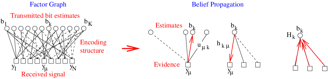
The bandwidth is discretized as time-frequency blocks (chips), so that a vector describes the spreading pattern across the bandwidth. Each users (labelled by ) is assigned a modulating code () for transmission/detection of a random bit, sent to/from a base station. The channel load is , which is finite. Consider the transmission case where the base station has knowledge of all codes in use. A superposition of the user transmissions, along with noise () arrives at the base station as shown in figure 1. Assuming perfect synchronization of the user transmissions with the chips the received signal on each chip is
| (1) |
where is the user specific fading, which may, in practical applications, be different for each chip and user. In order to allow good decoding the base station may coordinates the amplitude of codes so that in expectation the received Signal to Noise Ratio (SNR) is uniform for all users, which is a special case of power control. For example, users at greater distances (suffering greater fading) in a real cellular phone network will be instructed to use a higher transmission power to mitigate this effect. We assume such a determination of relative power levels has been achieved, so that we may take and normalized codes , the normalization can be taken without loss of generality in the analysis since the noise power spectral density can be rescaled accordingly. If the noise distribution is independent and Gaussian distributed on each chip then the SNR per bit is identical for all chips and defined as
| (2) |
where is the variance of the noise per chip. Note that the total signal to noise ratio (the power spectral density) contains an extra factor of .
1.0.2 Sparse, dense and composite spreading codes
In standard dense CDMA a code is assigned to each user so that on any chip the signal transmitted is modulated according to , which is non-zero for most or all chips. The Binary Phase Shift Keying (BPSK) random ensemble takes for each user a normalized code sampled uniformly at randomly from .
In one definition of sparse CDMA, by contrast, there is no transmission by user except on some finite subset () of chips (). Let be be the mean connectivity users in the ensemble, which is small and finite for the ensembles we study. The simplest case to consider is one in which the set is sampled independently and uniformly from the set of choose possible chip combinations for each user. Throughout this paper we consider the number of accesses for all users to be identical . For the subset of chips transmitted on by user (), in the standard case, BPSK modulation is used so that is sampled uniformly from .
To assume the number of accesses per user is a random, sampled from a Poissonian distribution, would also seem a natural choice, but note that with this choice some users will fail to access the bandwidth altogether. These disconnected users would strictly limit performance, and constitute a fraction of all users. Choosing the uniform distribution allows uniform access to the bandwidth for all users in expectation, and we expect this to be optimal in many senses [4].
In both cases the modulation method is BPSK. This is not the only viable modulation method, other simple modulation methods may result in improved performance [10]. One convenient simplification in the case of BPSK is the symmetry of the modulation, which means that for purposes of analysis the transmitted bit sequence can be chosen as (all 1’s) without loss of generality.
The codes we shall consider in this paper are composite codes which may be constructed as a sum of a sparse and dense codes sampled according to the definitions of this section. The composite code is sketched in figure 2, it involves both a sparse and dense random codes with power normalized to . The power ratio between the sparse and dense parts is controlled by a parameter , the spreading code may be written in this case as
| (3) |
If the sparse and dense codes are normalized the new code will be normalised up to a small () factor which is not important in the large system analyses. In the finite systems we correct for this difference.
The difference between composite and dense codes is in the hierarchical nature of the modulation sequences, all chips are transmitted on, but with two scales of transmission (provided ), so that in terms of information transmission and decoding the subset of chips for user does not become insignificant as becomes large, as would be the case for any subset of the chips given a dense code for user .
1.0.3 The case for random codes
Random codes, sampled according to some ensemble description, offer flexibility in managing bandwidth access by allowing code assignment by independently sampling for each user, and also have robust self-averaging performance for large system sizes. Furthermore the unstructured nature of codes makes them useful in adversarial models of communication, or in the presence of structured noise effects.
Random codes, sampled independently for each user, interfere in the channel. Optimal encoding of sources would involve a correlation of codes so as to minimise MAI. It has been shown that standard dense and sparse random codes can achieve a comparable to optimal transmission methods in the AWGN vector channel with only a modest increase in power. Optimal is here by comparison with transmission in the absence of MAI, the single user case, with comparable energy per bit transmitted. The small increase in power required to equalise performance is often a tolerable feature of wireless communication.
CDMA methods can be formulated so as to reduce or remove MAI; for example orthogonal codes () can be chosen for sparse and dense systems, whenever , achieving a single user channel performance. Gold codes [11] are the structured generalization of this beyond in the case of the dense ensemble, where the distance between codewords is maximized, but some MAI is present. A sparse version of the orthogonal case is Time or Frequency Division Multiple Access (TDMA/FDMA), whereby each chip is accessed by at most a single user. For (but sparse, ) improvement is also possible beyond the random ensemble – for example by enforcing the chip connectivity to be regular [4].
In many cases only limited coordination of codes might be possible, so that MAI is an essential and irremovable feature. Random code ensembles are used in this paper; with random MAI present implicitly. The composite code ensemble, like sparse and dense cases, has a structure which is suitable to detailed mean-field type analysis in the spread-spectrum limit, and as will be shown, can outperform sparse and dense analogues in some reasonable parameterisations of the linear vector channel.
The random coding models, with a little elaboration, may also approximated different scenarios other than ones corresponding to deliberately engineered codes. Consider for example a TDMA code, which is a sparse orthogonal coding method, so that the transmitted signal for any user is intended for a unique chip (time slot). In a practical environment this code may not arrive perfectly but might have a significant power component delayed by random processes, which contributes to unintended chips. This may occur in practice by way of multi-path effects [12]. In terms of the optimal detection performance, the properties may more closely resemble sparse CDMA, rather than a MAI-free TDMA method. If the paths are more strongly scattered across a significant fraction of the bandwidth a random dense inference problem is implied. Finally, a scenario with a few strong paths and many weak paths may apply, then the detection problem might be best approached as something similar to the composite code model.
1.0.4 The case for a statistical treatment
The large (spread-spectrum) scenario is an efficient multi-user transmission regime [13], and one in which we expect typical case performance of different codes drawn from our ensemble to converge. In the large system limit the typical value for performance statistics, that describe accurately almost all samples, are the quantities of interest. Taking finite the properties of dense, sparse and composite random codes are distinguishable and may be calculated from a free energy density. The spread-spectrum and many user limit is a standard benchmark, and statistical mechanics methods are established tools in analysis of such cases [14]. Often systems of practical size reflect strongly the properties inferred from the large system result; however, finite size effects may be critical in some practical issues of decoding.

2 Method
2.1 Calculation of Optimal Performance
To determine optimal performance we analyze the mutual information between the sent bits and received signal per bit . In the large bandwidth limit and for typical bit sequences, channel noise and code samples performance will be indistinguishable from the mean quantity
| (4) |
Where for our ensemble we will take . This quantity is expected to be self-averaging with respect to typical instances of the code. Self-averaging assumes that cases differing significantly from the mean value become statistically negligible as becomes large. The mean of the mutual information with respect to these quantities is then a sufficient measure of equilibrium properties.
This quantity may be most concisely determined through a statistical mechanics methodology. The probability distribution should be separated into a noise part, which is marginalised over, and a bit estimate part, which is the part of interest
| (5) |
For decoding purposes we assume an AWGN model, with signal to noise ratio per bit estimated as ( abbreviating SNR in equations), and marginalize with respect to this distribution to find a quadratic form in the exponent. The assumed form is within our model system correct, but in more complicated systems the form may still be used as an estimate. The prior is on bits is assumed to be uniform. The analysis then becomes equivalent to evaluation of an Ising spin model with Hamiltonian
| (6) |
and inverse temperature . The dynamical variables approximate the random variables , using the evidence and the code (quenched variables). The mutual information is affine to the free energy density for this model and takes an upper bound of bit.
The free energy may be evaluated through the replica method [9]. The self averaging free energy, averaged over code samples and instances of the channel noise, may be calculated by use of the replica identity
| (7) |
To apply the method we take as an integer, with becoming a product of partition functions in different dynamical variables, but shared quenched variables [15]. For each of the replicated partition functions a Gaussian identity may be applied to reduce the square in the exponent to a linear form
| (8) |
Representing as a product of the quenched variables , and and then separating those parts of order in the exponent (due to the dense code), we have
| (9) |
The sparse and dense code parts are now factorized in the exponent and the quenched averages may be made independently according to standard sparse and dense methodologies [4, 2, 10]; introducing order parameters for the sparse and dense induced correlations independently we have the free energy in a variational form (10). The energetic ( dependent) and entropic parts are separated for clarity, and the entropy has been assumed extensive. Assuming a Replica Symmetric (RS) form for the order parameters the free energy is determined by an extremisation
| (10) | |||||
| (11) | |||||
| (12) | |||||
The order and conjugate (hatted) parameters are and , normalized distributions over real fields, and , which are scalars. The averages are with respect to: , a Poissonian distribution (the excess chip connectivity distribution of the sparse sub-code), , a uniform distribution on (the modulation sequence), and , a normally distributed variable. Parameters
describe the assumed and correct signal to interference [channel noise and dense sub-code interference] ratios, respectively. If is not taken as the Nishimori temperature, , then .
The sparse code requires a full distribution to describe the contribution to the free energy, whereas the dense part requires only a few scalar parameters. Taking the limiting cases of large or small one set of order parameters becomes negligible and the usual sparse/dense expressions are recovered [4, 2]. The complexity of evaluating the free energy is limited primarily by the sparse part.
At the Nishimori temperature, corresponding to the correct detection model (), the free energy is correctly described by the RS assumption [16]. With this assumption we can make use of a symmetry to reduce the number of order parameters in the dense part (,). Extremization of the free energy leads to the following sets of saddle-point equations in the order parameters.
| (13) |
where the distributions by which averages are taken are unchanged. The quantity is a local mean field partition sum, only the dependence on one summation variable is written explicitly,
| (14) |
Equations are easily modified to include the general case.
From the free energy at the saddle-point, by application of small conjugate field against the terms , it is possible to identify with the distribution of log-posterior ratios of source reconstruction in typical instances of the quenched model. Let
| (15) |
then the quantity
| (16) |
once an analytic continuation is taken in the sum. From this observation the bit error rate is determined by the integral
| (17) |
The mutual information, with regards to typical case of (5), is attained by an affine transformation of the free energy. The entropy is also calculated from the same treatment, at the Nishimori temperature the energy is .
2.2 Decoding: multistage detection and BP
The idealized achievable performance is calculated in the limit of large under the RS assumption. In practice one must deal with finite systems, and the finite size effects tend to degrade performance relative to the ideal. However, for reasonable size systems () and the properties of composite codes in decoding, based on suitably constructed heuristics, become distinguishable from the performance through sparse or dense decoding methods, and approach in many cases the solutions predicted by the replica method.
We consider two algorithms, the standard multistage detection (MSD) [1], based on iteration of a vector approximation to the sent bits
| (18) | |||||
and a modified form of BP. MSD is a heuristic method [1], which works well in dense codes and simple noise models, provided MAI is not too large. BP is based on passing of conditional probabilities (real valued messages) between nodes in a graphical representation of the problem [17] (a schematic description of the method appears in figure 3).
The most time consuming step in BP is a trace over the states attached to a particular factor node in order to determine the evidential message, a naive approach in the dense case requires floating point operations. However, due to the central limit theorem the dependence on the weakly interacting bits, not connected strongly through the sparse code, is equivalent to a Gaussian random variable and the marginalization is replaced by an exact Gaussian integral. This reduces algorithm complexity asymptotically to .
The approximation leads to a more concise form for the evidential messages (passed from factor nodes to variable nodes):
| (19) | |||||
| (20) | |||||
| (21) | |||||
| (22) |
where a further simplification is possible for messages passed along dense links, using an expansion to leading order in ,
| (23) |
as constructed in [18]. In these expressions the notation indicates those equations where some corrections have been eliminated, the most critical being the replacement of the full marginalization over densely connected variables in (21) by a Gaussian integral that is taken analytically. At termination time the set of bits is determined by . Evidential messages may be combined in a standard way to give marginal log-posterior estimates for the source bits
| (24) |
and variable messages (passed from variable nodes to factor nodes)
| (25) |
The algorithm remains , and is less convenient than (18); however, the expression may be manipulated without introducing any additional errors at leading order in to an algorithm without dense messages [10], the manipulation is an application of that proposed in [19]. The asymptotic complexity of the algorithm is comparable to MSD and other good algorithms, although this disguises a large constant factor and some structures which might be difficult to implement efficiently in hardware.
Composite BP is applied as a heuristic algorithm based on an unbiased initialisation of the messages, in the hope that the various simplifications on the algorithm do not produce strong finite size effects. BP exactly describes the marginal probability distributions only if the messages (19), (23), (25) converge to a unique fixed point, since in this case describe the log-posterior ratios. There are two scenarios to be concerned about, either the BP messages fail to converge, or they converge to an incorrect fixed point - both scenarios occur in different decoding regimes for CDMA. The requirements for standard BP to successful decode are closely related to the assumption of RS, hence the similarity of the minimization process for (13) and the BP equations.
In studying systems of finite size we consider two message update schemes for both MSD and BP. The first is a parallel update scheme where all variables are updated such that the values of the current generation of messages () are conditionally independent given the previous generation of messages . The second schemes is a random stochastic update method, the updates are applied to all messages in the population, but in a random order. As soon as a variable is updated it is made available to subsequent updates, the messages in a single generation () are then not conditionally independent given the previous generation (). The sequential update method is slower to implement, but helps to suppress oscillations observed in some parallel update schemes, that lead to unphysical solutions.
A measure of convergence for the BP is the mean square change in variable states
| (26) |
whereas the convergence measure for MSD is similar but with the log-likelihood ratios replaced by the bit estimates. An exponential decay in this quantity, or an evaluation to zero, would be characteristic of a convergent, or converged, iterative method.
2.3 Properties of decoders in finite systems
MSD is an iterative method which works very well in systems with small load and mixing parameter . In the first iteration the achieved result is equivalent to a matched filter. In subsequent iterations the estimates are updated, but because the information is rather crudely used the consequence can be instability of the iterative procedure. For instance, the examples shown later reveal very poor performance of MSD when MAI is large. Since MSD is based on filtering it is not so successful for composite ensembles as for dense ones, and its reliability in dense codes improves as system size increases.
The critical scenario in which BP is guaranteed to produce the correct marginal posteriors is that the graphical model is tree like (see figure 3). However, BP often produces a reasonable performance in loopy models including sparse [6] and dense [19] CDMA. The failing regime in BP corresponds to large in the sparse and dense codes, but at intermediate the instabilities appear to be worse, or new instabilities are apparent.
In many of the cases studied we found that BP did converge in the marginal log-likelihood ratios, this was the case for systems at small , and/or high SNR. In other cases the fields did not converge, and instead a steady state was reached at the macroscopic level – remembering the BP equations describe a dynamic algorithm, which does not obeying detailed balance, this might be expected. The steady state is one in which the distribution of messages converges up to finite size effects, but the individual messages do not converge. Steady states were characteristic of systems initiated with random or unbiased messages at high . The estimates determined from the distribution of messages in the steady state typically corresponds to a high estimates.
In regimes where message passing is unstable the detectors may still be used to provide an estimated, subject to some termination criteria. Variations on MSD and BP involving heuristic tricks may avoid some of these effects, but some of the standard methods may be unsuitable to the composite model. Experimenation with the update scheme demonstrated improved results in MSD for example.
The dynamics of numerically solving the saddle-point equations (13) are very closely related to the iteration of BP. The dynamics of the iterations (figure 5) appear smooth and systematic even at large based on a numerical solution involving points. However, in addition to the use of a large system size, control was exercised over finite size effects through selective sampling of quenched variables in the update step (19), which is not possible in BP. Therefore any realisation of the problem in BP, even at an equivalent system size, is not expected to produce such uniform effects. Many qualitative features such as the speed of convergence appear to be reproduced in some of our finite realisations.
Naturally we expect there to be finite size effects, the trends presented appeared consistent across a range of system size from to chips. No structured attempt is made to calculate these effects, or to distinguish the contributions due to the different approximations in the algorithm and other instabilities implicit to BP. Working with a sufficiently large graph is problematic since the algorithm is asymptotically rather than linear, and it is necessary to store and manipulate a modulation pattern matrix.
2.4 Replica symmetry and the phase space
At the Nishimori temperature the RS solution is guaranteed to describe correctly the thermodynamically dominant states. Across a range of parameters we find two saddle-point solutions: one corresponding to a locally stable bad solution (bad decoding performance) and one to a locally stable good solution (good decoding performance). The metastable solution (solution producing the higher free energy) is irrelevant in determining the equilibrium properties since it does not contribute to the free energy at order . However, in terms of dynamics or local sampling the bad solution can be dominant even where it does not describe the equilibrium phase. We find these metastable regimes at intermediate SNR and high MAI (above [2]).
The RS solution obtained at equilibrium appears sufficient to describe the good equilibrium and metastable solutions. These are the local solutions to the free energy that correspond to states clustered about the encoded bit sequence . In this case the phase is connected in state space, and so we expect the dynamics of the system to be relatively simple, so that the phase space can be explored by local sampling methods such monte-carlo. BP will be locally stable in the vicinity of this solution, in the absence of competing local minima we can expect convergence towards this in specific realisations. This solution to the free energy exists when SNR is sufficiently large.
By contrast we expect there to also be a bad (liquid/paramagnetic) equilibrium solution when SNR is small. The field term in the Hamiltonian means the magnetisation is never zero, but we expect there to be a suboptimal ferromagnetic solution which is also connected in state space, and that has similar properties in terms of BP and sampling. The good and bad equilibrium solutions are guaranteed to have simple phase space structures described by RS, this conclusion and some thermodynamic properties can be calculated without the replica trick or cavity method [16].
Finally we can anticipate that at high MAI and intermediate noise there may be a bad metastable solution. The bad metastable solution emerges continuously from the bad equilibrium solution with increasing SNR and so will be characterised by a connected phase space for some parameters. However, as the noise decreases we might expect this solution to become fragmented and the RS metastable solution to become unstable, but this instability is not tested. An indication of the failure of RS is the negative entropy in some metastable solutions, which is not viable. It is not uncommon for systems with simple connected phase spaces to exhibit negative entropy when the RS ansatz is applied under the assumption of extensive entropy [20], as we employ in the calculation. A result without negative entropy can be formulated by a minor variation on the RS approach called frozen replica symmetry breaking (RSB), which effectively rescales the temperature. However, it is not certain that this solution will be correct without a local stability analysis towards other forms of RSB, in many other systems negative entropy is one indicator of a failure of the connected phase space assumption [15].
In the bad metastable state, and also in the bad equilibrium phase away from the Nishimori temperature (), the connected description is possibly incorrect even where the entropy is positive; an RSB formalism may be applicable. The good solution is likely to be well described by RS at all temperatures, since it is a state clustered around the encoded bit sequence. For the RS approximation produces a variational approximation to the thermodynamic behavior. The RS approximation can also describe exactly the metastable states in some regimes, but this is not the case in general.
The hypothesis of a connected state described by the RS treatment has consequences for dynamics, as do the various hypotheses on the nature of RSB, should it occur either in a search for the ground state [21], or at some intermediate temperature. On specific realizations of graphs we might expect BP to converge for the states correctly described by RS. However, in finite graphs we might expect strong finite size effects to dominant behaviour, so that in the absence of a scaling analysis conclusions cannot be drawn directly from simulation results. In cases where BP is unstable due to RSB or finite size effects we might nevertheless expect to uncover a steady state of the dynamics that is strongly correlated with nearly optimal solutions and is useful for extracting an estimate of sent bits.
3 Results
3.1 Parameters considered
The model constructed is already quite simple, avoiding some of the practicalities of real channels and making no attempt to optimize for finite size effects in the composite ensembles. However, even with these simplifications the channel produces interesting behavior. In order to demonstrate the equilibrium properties of composite codes in such a way as to produce strong contrast between the ensembles we work with systems with and between and . Beyond this range of results appear by experimentation to be very much a continuation of the trends highlighted.
Analysis of the sparse code () is for this range of parameters a loopy inference problem, but is sufficiently far from the percolation transition to be well behaved. At the same time is sufficiently small to allow quick decoding and produce a contrast with the dense code. It has been noticed since the early days of studying sparse codes that the mean connectivity of the sparse code ensemble does not have to be very large at all for results to become indistinguishable from the dense code [3, 22].
A lower bound to the achievable bit error rate in all ensembles is given by the single user Gaussian channel (SUG) result over a bit interval
| (27) |
which is the complementary error function of SNR. In the absence of MAI this lower bound can be achieved if spreading patterns are coordinated so as to be orthogonal. On the vector channel this orthogonality is possible only if , unavoidable MAI at higher loads will strictly degrade performance.
The saddlepoint equations (13) are solved by population dynamics [23], an iterative method for solving the saddle-point equations using a histogram approximation of the distribution ( points are sufficient to attain our results). Evolving the order parameters from initial conditions that correspond to low and high finds either the unique solution or a pair of locally stable solutions.
3.2 Equilibrium behavior of unique saddle-point solutions

Generally with there is a unique solution of the saddle-point equations with a smooth transition between bad and good solutions as SNR is increased. The population dynamics equations require very few iterations and results can be achieved with relatively fewer points in the histogram. The normal working range of CDMA is often by design one with a relatively small load () and so falls into this class of behaviour.
The trends in for the large system limit for are demonstrated in figure 4. The dense code ensemble achieves a smaller bit error rate than the sparse code ensemble, and the composite code ensembles interpolate between these. With the curve is indistinguishable at this magnification from the dense curve, with balanced power in the two codes performance resembles the dense code. At intermediate SNR there is a large gap in BER, which narrows in the limits of high and small SNR. Trends in the free energy follow a similar monotonic pattern – the dense code has the highest mutual information everywhere.
3.3 Metastable solutions of the saddle-point equations


The regime of high is of greater theoretical interest in multi-user detection since this is where MAI causes results to differ substantially from single user models. As is increased beyond a spinodal point may be reached beyond which there are multiple locally stable solutions to the saddle-point equation.
In regimes with a competition between locally stable attractors, or with one marginally stable attractor convergence of the saddlepoint equations is slowed down; one such scenario is shown in figure 5. At there is a unique solution for some of the sparse and composite ensembles, but not for the dense ensemble. In this example the composite code solution is superior to the sparse solution, and the dense metastable (bad) solution. The best solution is the dense thermodynamic (good) solution. As shown in figures 6 and 5, the entropy is positive for all the thermodynamic solutions. However, at larger and higher SNR the metastable solutions can have negative entropy, indicating an inadequacy in the RS description.
The saddle-point solutions for our ensembles with load at a range of SNR is shown in figure 6. For this load metastability is present at all values. Where the solution is not unique the correct and metastable solutions can be distinguished from the free energy (equivalently entropy at the Nishimori temperature). At the Nishimori temperature there is a second order transition, the energy is equal to in both solutions, which is realized as a discontinuous transition in the BER. In the metastable regimes we find the entropy evolves towards a negative value as SNR increases, the correct metastable state in the negative entropy regime is described by the state space at the freezing point where entropy first becomes negative.
Up to 7dB the bad solution is the thermodynamic solution in all ensembles. Close to the transition the best performing codes are composite ones with , but at lower SNR the regular code ensemble appears best. The composite systems displayed all have thermodynamic transitions near 7dB, the entropy and free energy of the sparse bad solution is much larger, so that thermodynamic transition does not occur until about 9.5dB. This entropy gap is a clear feature of the local freedom explicit in a sparse connectivity model and absent in the composite one. In the case of a regular sparse part, with a more homogeneous interaction structure, the gap in entropy and thermodynamic transition point are significantly reduced [4]. Amongst the good solutions, in contrast to the bad solutions, both the ensemble entropy and appear to be ordered by for all SNR.
The metastable solutions appear to be qualitatively similar in the composite ensemble to the sparse and dense ensembles [19, 4]. What is interesting in the metastable regime is that the positioning of the composite state performance is not a simple interpolation between the sparse and dense ensemble results. In the example shown the metastable solutions for composite codes are at lower than either the sparse or dense metastable solutions. Furthermore, for there is a unique solution beyond 8dB inspite of the persistence of metastable solutions in the sparse and dense ensembles at significantly larger SNR.
We did not test the microscopic stability of the metastable solutions for the composite system, but this should be possible, in part, by a local stability analysis of the RS description. It is expected that at, and above, the Nishimori temperature () the RS description will be locally stable even for the metastable states, as was found for the dense and sparse codes [19] [4].
The composite codes exhibit a thermodynamic behaviour most strongly contrasting with both sparse and dense codes when , and close to the thermodynamic transition of the dense code. The effect of distributing power mostly in the sparse code appears to destabilise the bad solution in some marginal cases. Results obtained by the replica method solved by population dynamics appear robust; only close to the dynamical transition points, where solutions are marginally stable, are not well represented.
To understand the origins of this instability requires a more detailed investigation of the stability of the RS metastable solutions, and possibly an RSB type treatment. We suspect that the dense code behaves comparably to the external field at equilibrium, and this might be one way in which one could approach the problem.
3.4 Decoder Performance


In systems with the equilibrium results are achievable by iteration of BP equations, this was established previously for the dense case in [19]. Such an example is shown in Figure 7 with . The performance of MSD is poor, although initially the achieved bit error rate is improving with each iteration, over many iterations there is a clear oscillation. For systems of higher SNR and/or decreased we find the MSD result to be very close to BP and the theoretical result. The BP algorithms reproduce the equilibrium result to within a small error after only a few iterations, even in systems with only users and chips (), across a range of . Where unique saddle-point solutions were predicted by the equilibrium analysis decoding by BP normally produced a stable fixed point. The MSD results are not shown in subsequent figures but are suboptimal with respect to BP in all cases.
A histogram of achieved BERs is demonstrated in figure 8. In the large system limit we would expect the cumulative distribution functions to converge towards step functions (self averaging) on the one of the thermodynamic solutions, but it is clear we are quite far from this scenario. BP converges quickly towards results of very low or zero BER. The MSD algorithm works very well, but more slowly than BP, for a subset of examples. In many other samples the performance deteriorates as MSD is iterated beyond the initial approximation (matched filter).
If we consider a similarly sized system of chips and users () then we can observe decoding performance in a regime which should be characterized by metastability in the dense code but not in the sparse code. The final achieved in samples for various systems is shown as a cumulative probability distribution in figure 9 after 10 iterations and after 80 iterations. The sparse system is unimodal, with fast convergence in most systems. The dense ensemble is multimodal as expected, the convergence time towards the low solutions are very slow, and the majority of achieved solutions are close to the high metastable solution. Random initial conditions tend to produce steady states characterized by the bad solution, even if this corresponds to the metastable rather than equilibrium solution. The composite system equilibrium solution is unique for . For some of samples improve between iteration and iteration , but also worsen, the median performance is quite far from the equilibrium value. The equilibrium results for are not closely approximated in the decoding experiments, the performance in is worse everywhere than the equilibrium prediction and the constituent dense and sparse systems. For large it appears the finite size effects are more limiting in the case of the composite codes, particularly at intermediate values of .
The composite systems shown in figure 9 does not come close to the performance of even the bad solution in either the median or mean for this system size except for large or small . The ability of the composite algorithm [18] is limited in achieving the equilibrium result for intermediate than standard methods for the sparse [6] and dense [19] ensembles for systems of this size. A quantitative comparison of the equilibrium and finite size systems in the metastable regime with bulk statistics such as the mean is difficult due to the multimodal nature of the distributions.
The decoder performance for systems of size seem to provide mean values for the BER, which are quite far from the theoretical values and unable to realise the advantages of some composite codes predicted by the equilibrium analysis. There are many approximations made at in construction of the BP algorithm [19] [18], which are both systematic and random, and it is possible these are at the root of the BP instability for intermediate values of . However, it is noteworthy that even without elimination of dense messages, performance with the proposed update schemes are poor at intermediate . The ordering of updates may also be important, and other sensible schemes might be consider. For example to iterate only the sparse messages until convergence (a fast process) between updates of dense message dependent quantities.
3.5 Regular sparse ensembles

A random ensemble with regular chip connectivity [4] as well as regular user connectivity will be examined. There is not a strong case for use of these codes in practical scenarios, but they offer the possibility to demonstrate a positive result for the composite system which is reproducible in small system size experiments.
An interesting alternative composite system to the user regular ensemble is one in which the number of accesses per chip (call this ) is equal for all chips. This requires global coordination of all users, with the loosening of this restriction neither the doubly-regular ensemble presented nor the random codes would represent the most high performing options. However, the regular code is interesting because it shares many of the topological features of the sparse random ensemble, but has very slightly lower MAI, reduced by a factor [24] over the random sparse or dense ensemble, and fewer finite size effects in the BP algorithm. The reduced MAI has the effect that at low values for SNR the unique stable solutions for the doubly regular ensemble is superior in to the dense ensemble. With this ensemble one can demonstrate a statistically significant result, in decoding by BP, for which the composite code ensemble outperforms the corresponding sparse and dense parts in .
The equilibrium behaviour of the doubly regular sparse ensemble was analysed in [4]. Replacing the standard sparse code ensemble by the composite one we can repeat the replica analysis and use the same set of BP equations (identical at leading order). In the analysis we find that the composite code performance interpolates the sparse and dense performance in low and high SNR regimes. However, in an intermediate range of SNR, where the bit error rate is equal in the sparse and dense models, the unique solutions for the composite ensembles become superior to both the dense and sparse ensemble result. The performance of several ensembles is shown in figure 10.
Working with a simulation of users and chips we are able to demonstrate that the mean performance of several composite codes exceed the performance of there constituent parts, as shown in figure 11. The results for ensembles are close to the large system limit prediction, to within error bars. The composite code achieves the lowest bit error rate in expectation amongst the codes, and has convergence properties somewhere between the two extremal ensembles. As in previous experiments the performance for is much poorer than the large system limit prediction.
As can be seen the dense code fields are initially converging in a similar way to figure 7. However, at later time the fields appear to be becoming unstable again (at least for a subset of simulations that dominate the measure). This instability might be a direct consequence of the inaccuracy of the Gaussian BP approximation (21) when in decoding becomes very small. Similar trends are seen in some of the composite codes, often the messages do not converge exactly but only to with some fixed variability.

4 Discussion
The equilibrium analysis demonstrates that in regions of metastability the composite coding structure, comprising of a sparse and densely connected component, might have some interesting and valuable properties. When power is approximately equal in the two parts performance is very close to the dense ensemble, but with only a small amount of power in the dense code properties are strongly distinguishable. At the same time, we have shown that in reasonably sized simulations our algorithmic approaches based on O(1/N) approximations in the dense code prove to work relatively poorly in the composite codes. This instability in some composite codes can persist even in scenarios where the equilibrium analysis predicts a regime without a metastable solution, which would be the natural candidate for a non-equilibrium attractor.
We predict the failure of the composite BP algorithm to be in part related to the Gaussian approximation in marginalization over states (21), which may be a poor approximation when messages become strongly biased. If this is the case then the problem may be avoided or mitigated by standard algorithmic tricks such as annealing or damping. When the messages become very biased, replacing the full marginalization by one considering only a truncated set of states might be a viable polynomial time alternative to using the analytical Gaussian approach. In small realisations of composite systems many heuristics might be employed.
In the final section we presented results with a different type of sparse ensemble in which there was some coordination between users. Similarly there would be some value in considering either an ordered (optimised) sparse code combined with a random dense code or vice-versa. The ordered sparse code might provide a method for decoding under ideal channel conditions, whereas the dense code provides a contingency and some of the advantages of the spread spectrum approach. At least in so far as a practical method this might be a well-motivated scenario.
The composite code presents an interesting dichotomy in its surpression of the metastable behaviour, but greater apparent instability in simulation. Aside from standard convergence measures in simulations we have not thought of a concrete way to probe the origins of this instability in simulations. One possibility would be to study the equilibrium properties of the metastable state in more detail in the thermodynamic framework.
A finite size scaling of the algorithm results would be valuable, unfortunately the need to manipulate an by dense spreading matrix restricts us somewhat in moving to larger scales. The scales we have presented, and error bounds, are presented in a somewhat ad-hoc way but this is only to demonstrate the breadth of behavior. Many results in the cited papers go much further in dealing with the question of finite size effects in sparse and dense systems.
We have developed a method which is applicable where the sparse ensemble includes graphs which are fully connected. If we consider a composite code with a sparse part below the percolation threshold a more fruitful analysis might consist in a two level analysis. By considering the different classes of disconnected components (within the sparse code) as the microscopic states connected through a homogeneous (dense code) interaction. This may also be the basis for better algorithms.
Acknowledgements
Support from EPSRC grant EP/E049516/1 is gratefully acknowledged (DS).
References
- [1] S. Verdú. Multiuser Detection. Cambridge University Press, New York, NY, USA, 1998.
- [2] T. Tanaka. A statistical-mechanics approach to large-system analysis of CDMA multiuser detectors. IEEE Trans. on Info. Theory, 48(11):2888–2910, Nov 2002.
- [3] M. Yoshida and T. Tanaka. Analysis of sparsely-spread CDMA via statistical mechanics. In Proceedings - IEEE International Symposium on Information Theory, 2006. (Seattle), pages 2378–2382, Piscataway, NJ, USA, 2006. IEEE.
- [4] J. Raymond and D. Saad. Sparsely spread CDMA - a statistical mechanics-based analysis. J. Phys. A, 40(41):12315–13334, 2007.
- [5] D. Guo and C. Wang. Multiuser detection of sparsely spread CDMA. IEEE J. Selected Areas Commun., Special Issue on Multiuser Detection for Advanced Communication Systems and Networks, 26(3):421–431, 2008.
- [6] A. Montanari, B. Prabhakar, and D. Tse. Belief propagation based multiuser detection. In 43rd Annual Allerton Conference on Communication, Control and Computing 2005. (Monticello), Red Hook, NY, USA, 2006. Curran Associates, Inc.
- [7] J. Raymond and D. Saad. Composite systems of dilute and dense couplings. J. Phys. A, 41(32):324014 (30pp), 2008.
- [8] M. O. Hase and J. F. F. Mendes. Diluted antiferromagnet in a ferromagnetic environment. J. Phys. A, 41(14):145002 (9pp), 2008.
- [9] H. Nishimori. Statistical Physics of Spin Glasses and Information Processing. Oxford Science Publications, Oxford, UK, 2001.
- [10] J. Raymond. Typical case behaviour of spin systems in random graph and composite ensembles. PhD thesis, Aston University, Birmingham, UK, November 2008.
- [11] R. Gold. Optimal binary sequences for spread spectrum multiplexing (corresp.). IEEE Trans. on Info. Theory, 13(4):619–621, 1967.
- [12] T.S. Rappaport, S.Y. Seidel, and R. Singh. 900-MHz multipath propagation measurements for U.S. digital cellular radiotelephone. Vehicular Technology, IEEE Trans. on, 39(2):132–139, 1990.
- [13] V. Ipatov. Spread Spectrum and CDMA. Principles and Applications. John Wiley & Sons, Hoboken, NJ, USA, 2005.
- [14] D. Guo and S. Verdú. Communications, Information and Network Security, chapter Multiuser Detection and Statistical Mechanics, pages 229–277. Kluwer Academic Publishers, Norwell, MA, USA, 2002.
- [15] M. Mézard, G. Parisi, and M.A Virasoro. Spin Glass Theory and Beyond. World Scientific, Singapore, 1987.
- [16] H. Nishimori. Comment on ”Statistical mechanics of CDMA multiuser demodulation” by T. Tanaka. Eur. Phys. Lett., 57(2):302–303, 2002.
- [17] F.R. Kschischang, B.J. Frey, and Hans-Andrea Loeliger. Factor graphs and the sum-product algorithm. IEEE Trans. on Info. Theory, 47(2):498–518, 2001.
- [18] E. Mallard and D. Saad. Inference by belief propagation in composite systems. Phys. Rev. E, 78(2):021107, 2008.
- [19] Y. Kabashima. A statistical-mechanical approach to CDMA multiuser detection: propagating beliefs in a densely connected graph. In Proceedings - IEEE International Symposium on Information Theory 2003. (Yokohama), page 329, Piscataway, NJ, USA, 2003. IEEE.
- [20] D.J. Gross and M. Mézard. The simplest spin glass. Nuclear Pnys. B, 240:431–452, 1984.
- [21] F. Krzakala, A. Montanari, F. Ricci-Tersenghi, G. Semerjian, and L. Zdeborová¡. Gibbs states and the set of solutions of random constraint satisfaction problems. Proceedings of the National Academy of Sciences, 104(25):10318–10323, 2007.
- [22] A. Montanari and D. Tse. Analysis of belief propagation for non-linear problems: The example of CDMA (or: How to prove Tanaka’s formula). In Proceedings IEEE Workshop on Information Theory. (Punta del Este), pages 160–164, Piscataway, NJ, USA, 2006. IEEE.
- [23] M. Mézard and G. Parisi. The Bethe lattice spin glass revisited. Eur. Phys. Jour. B, 20(2):217–233, 2001.
- [24] J. Raymond and D. Saad. Randomness and metastability in CDMA paradigms. In Modeling and Optimization in Mobile, Ad Hoc, and Wireless Networks and Workshops, 2008. WiOPT 2008. 6th International Symposium on (Berlin), pages 626–630, Piscataway, NJ, USA, 2008. IEEE.