789\Yearpublication2006\Yearsubmission2005\Month11\Volume999\Issue88
Turbulent stresses as a function of shear rate in a local disk model
Abstract
We present local numerical models of accretion disk turbulence driven by the magnetorotational instability with varying shear rate. The resulting turbulent stresses are compared with predictions of a closure model in which triple correlations are modelled in terms of quadratic correlations. This local model uses five nondimensional parameters to describe the properties of the flow. We attempt to determine these closure parameters for our simulations and find that the model does produce qualitatively correct behaviour. In addition, we present results concerning the shear rate dependency of the magnetic to kinetic energy ratio. We find both the turbulent stress ratio and the total stress to be strongly dependent on the shear rate.
keywords
accretion, accretion disks – instabilities – magnetohydrodynamics (MHD) – turbulence1 Introduction
Since the work of Balbus & Hawley (1991) it is now generally accepted that turbulence in accretion disks is caused by the linear magneto-rotational instability (hereafter MRI) that was originally discovered by Velikhov (1959) in connection with Couette flow of liquid metals. This linear instability can be excited in sufficiently ionized, differentially rotating fluids where the angular momentum decreases with increasing radius. When the fluid is threaded by a magnetic field, differential rotation causes stretching of the field lines. The tension that builds up opposes the shearing, acting to enforce rigid rotation. If the field is subthermal, the interplay between differential rotation and magnetic tension destabilizes the fluid, resulting in linear growth of Reynolds and Maxwell stresses, which transport angular momentum outwards. The instability eventually leads to a fully turbulent, non-linear state.
Let us assume a rotation profile of the form , where is the angular velocity at distance . A necessary condition for the MRI to be excited is , i.e. the angular velocity decreases outward. The Keplerian case with has been extensively studied by means of numerical simulations making use of the shearing box approximation (e.g., Hawley, Gammie & Balbus 1995, 1996; Brandenburg et al. 1995; Johansen & Klahr 2005), as well as in global disks (e.g. Armitage 1998; Hawley 2001; Lyra et al. 2008). These studies have shown that the MRI leads to a fully turbulent saturated state in which the Maxwell stress is responsible for the majority (about 80%) of the angular momentum transport. Even in the absence of vertical density stratification a turbulent small-scale magnetic field can be maintained by dynamo action (Hawley et al. 1996). When stratification is present, cyclic large-scale dynamo action can be excited (Brandenburg et al. 1995).
The dependence of Reynolds and Maxwell stresses on the shear rate has been investigated numerically by Abramowicz, Brandenburg & Lasota (1996) in the presence of stratification and Hawley, Balbus & Winters (1999) in the absence of stratification. It turns out that near the Reynolds stress, which couples to the large-scale vorticity , is small due to the strong stabilizing effect of the vorticity (Hawley et al. 1999). This makes the Maxwell to Reynolds stress ratio very high. As the shear rate increases, the shear-coupled Maxwell and Reynolds stresses increase due to the decrease of the vorticity. However, the growth of the Reynolds stress is significantly faster, so the stress ratio diminishes with increasing .
The interest in MRI-generated turbulent stresses as a function of was rekindled in a recent study where a linear analysis of the Reynolds and Maxwell stresses was presented (Pessah, Chan & Psaltis 2006a, hereafter PCP06). They derived a simple relation for the stress ratio, depending only on the shear parameter . Comparing this result with the non-linear simulations of Hawley et al. (1999), they find that, even in the saturated turbulent regime, the stress ratio does indeed depend almost entirely on alone, and that there is only a weak dependence on other properties of the flow or on the initial conditions.
The Shakura-Sunyaev viscosity parameter (Shakura & Sunyaev 1973) is still a popular tool to link accretion disk observations to theory. The so-called model of disks is based on the assumption that the turbulent stresses scale linearly with the thermal pressure; being the proportionality factor. In this formalism, the outward transport of angular momentum is characterized by a turbulent viscosity of the form
| (1) |
where the eddy viscosity is assumed to scale with the sound speed and the correlation length with the disk scale height .
As this model linearizes the turbulent system into a standard Navier-Stokes fluid suitable for analytical manipulation, it has been an invaluable tool in developing theory of accretion disk dynamics, even though the parametrization offers no explanation of what is causing the viscosity. Even after the realization of the astrophysical importance and subsequent reinvigorated interest in the theory of the MRI, the -model is still widely used.
New, more physically motivated models have been developed recently to describe the angular momentum transport in accretion disks (e.g. Kato & Yoshizawa 1995; Pessah, Chan & Psaltis 2006b; Ogilvie 2003, hereafter O03). A common characteristic of these models is the treatment of the problem of angular momentum transport: the governing magnetic and kinetic equations are divided into linear and non-linear terms. The non-linear correlation functions are then modelled by closing the system of equations with approximate expressions that still embody the physics but are considerably easier to solve (such closure models are commonly used in modelling turbulence; see references in O03). It should be noted that the -model is mathematically equivalent to the simplest closure model, where the correlation functions are modelled by one single coefficient. All these models also operate in the absence of mean magnetic fields. A first attempt to validate the O03 model was made by Garaud & Ogilvie (2005) in connection with shear flow where linear and non-linear instabilities were found to be well reproduced by the model.
In the present study, the turbulent stresses are extracted as functions of from non-stratified local numerical models with zero net flux using the shearing box approximation. The simulation data are compared with the linear results of PCP06 and the non-linear closure model of O03. There are a few other closure models that describe the behaviour of local, magnetohydrodynamic turbulence. In particular, the model of Pessah et al. (2006b) assumes a uniform vertical field in the disk which is not incorporated in our three-dimensional simulations. Therefore we concentrate here mainly on the closure model of O03.
2 Stress ratio in the model of PCP06
Here we briefly summarize the formalism employed in the model of PCP06. Using the kinematic hydromagnetic equations, PCP06 calculated the ratio of the relevant components of Reynolds and Maxwell stresses in a local approximation. We use here a Cartesian frame of reference, where , and denote the radial, toroidal and vertical directions, respectively. The relevant component of the stress tensor is then , which can be decomposed as
| (2) |
where
| (3) |
are the Reynolds and Maxwell stresses, respectively, and is the departure from the mean flow, is the departure from the mean magnetic field, is the density, the vacuum permeability, and angular brackets denote a suitable volume average. Throughout our paper, compressibility effects are ignored in the turbulence models, i.e. is assumed constant, even through the simulations are fully compressible. The rms velocity in our simulations remains considerably smaller than unity and the flow is therefore subsonic.
Using linear theory, PCP06 found that for given wavenumber the stress ratio is given by
| (4) |
where is the angular velocity, is the Alfvén speed based on a constant vertical magnetic field, and is the corresponding growth rate of the mode with wavenumber . Moreover, for the fastest growing mode with
| (5) |
they find
| (6) |
This expression shows that, for the relevant case with , the magnitude of the Maxwell stress is always larger than that of the Reynolds stress. This formula provides a strikingly simple prediction of the stress ratio which is in good agreement with simulation data, even if there is no imposed magnetic field (PCP06). One envisages that the relevant wavenumber is able to adjust itself to the value where the growth rate is maximal.
3 The O03 closure model
The local closure model of O03 includes the linear interaction of the turbulent stress tensors with shear and rotation. The linearized evolution equations for the Maxwell and Reynolds stresses can be derived directly from the basic MHD equations and are fairly straightforward to solve numerically. For modelling the non-linear triple correlations of fluctuating quantities and the small-scale diffusion, five dimensionless, positive definite coefficients appear in the closed system of equations. A closure model is needed to deal with these non-linear terms which are described by physical effects and constrained by symmetry properties and dimensional considerations.
The five closure coefficients stand for the turbulent dissipation of the Reynolds stresses (), their isotropization (), the effect of the small-scale Lorentz-force as a source for combined with a sink for (), a source due to small-scale dynamo for combined with a sink for (), and turbulent dissipation of the Maxwell stresses ().
The evolution equations of this model are given by
| (7) | |||||
| (8) |
where is the turnover time, is the rms velocity, is the typical scale of the energy-carrying eddies, and
| (9) |
| (10) |
are the traces of tensors and . Furthermore, and are linear and nonlinear terms, respectively, for or , and are given by
| (11) | |||||
| (12) | |||||
| (13) | |||||
| (14) |
where is the ratio of rms magnetic and velocity fields,
| (15) |
is an isotropization term, and are positive constants that are of the order of unity. Advection operators of the form have been neglected. The contribution of the advection terms vanish under fully periodic boundary conditions on average so they make no contribution. Note also that and are time-dependent, because and are time-dependent.
A similar model for the hydrodynamic case has recently been used to to model the generation of shear in rotating anisotropic turbulence by the effect; see Käpylä & Brandenburg (2008) for details. An important difference is that in their model the flow was driven by an external body force, so the equations for the evolution of the Reynolds stress have a corresponding forcing term as well. Such a term is here absent, because the turbulence is solely the result of shear flow instabilities and are modelled by the equations of O03 without external forcing. As explained by O03, the model also predicts turbulence for , where simulations have not shown self-excited turbulence. The reason for this is that O03 do not specifically model the MRI dynamics.
In the present study the large scale velocity is given by the shear flow . We abbreviate the parameter combination of O03 by . O03 gave an analytic solution for the hydrodynamic case. Here we give a partial solution for the components of the two stresses if and are known. In the steady state, the equations yield for the Reynolds stresses
| (16) |
| (17) |
| (18) |
| (19) |
where we have introduced the abbreviations
| (20) |
and
| (21) |
The components of the Maxwell stress tensor can be expresses in terms of the corresponding components of the Reynolds stress tensor as
| (22) |
| (23) |
| (24) |
| (25) |
The remaining mixed components involving vanish, i.e. . When , there is an explicit expression for , derived by O03.
For the general case with , we did not find an analytic expressions for and in closed form. However, using the time-dependent equations it is possible to determine a linear fit of the form
| (26) |
| (27) |
where the are an approximation to the final fit parameters, and and are the corresponding numerically determined values of and . We are thus able to decrease the degree of freedom of the fitted system. We refine the parameters with respect to the initial “guess” based on the quantity
| (28) |
In the analysis we seek the minimum value of .
4 Simulations
For the simulations we adopt a cubic computational domain of size . The gas is isothermal with constant sound speed ; vertical gravity and stratification are omitted. The calculations are local and therefore made under the shearing box approximation (see below). The equations to be solved read
| (29) | |||||
| (30) | |||||
| (31) |
where includes the advection by the shear flow, is the departure from the mean flow , is the density, is the magnetic vector potential, is the magnetic field, and is the current density, is the vacuum permeability, is the traceless rate of strain tensor, is the kinematic viscosity, and is the magnetic diffusivity.
In order to get as close as possible to the ideal limit, we replace the diffusion terms by a hyperviscosity scheme, i.e. we replace the -operators by , aiming at maximizing the Reynolds number in the quiescent regions of the flow while diffusing and damping fluctuations near the grid scale. Compared to direct simulations (e.g. Haugen & Brandenburg 2006) with uniform viscosities, smaller grid resolution can be used to resolve the flow, which is crucial if the plan is to, e.g., undertake a parameter study, like in our case.
Periodic boundary conditions are applied in all three directions; in the radial direction we account for the shear flow by making use of the shearing box approximation (e.g. Wisdom & Tremaine 1988):
| (32) |
where stands for any of the seven independent variables, stands for the radial extent of the computational domain, and is the time.
The domain is initially threaded by a weak magnetic field,
| (33) |
where has been chosen, and is the smallest finite vertical wavenumber in the domain of height . Thus, the magnetic field contains periodic - and -components with amplitude .
We choose the values of , and so that the most unstable mode of the MRI, is well resolved by the grid; in practise this means that we always adopt , and , resulting in . For the initial setup, the other condition for the onset of MRI, namely , where is the ratio of the thermal to magnetic pressure, is also satisfied as is minimally 50 at the maximum values of the magnetic field. In all our runs the Mach number is well below unity, so compressibility effects are negligible.
For all the simulations we use the Pencil-Code11 1 http://www.nordita.org/software/pencil-code/, which is a high-order (sixth order in space, third order in time), finite-difference code for solving the MHD equations (Brandenburg & Dobler 2002).
The local calculations have been carried out at two different resolutions, namely (in 1D) and (in 3D); the corresponding numerical diffusion coefficients are and , respectively. The calculations were carried out on the IBM eServer Cluster 1600 at Scientific Computing Ltd., Espoo, Finland.
5 Results
5.1 Linear results
In order to make contact with the model of PCP06, we first aim at reproducing their theoretical linear results (see also Balbus & Hawley 1991) using one-dimensional calculations with an imposed magnetic field. We calculate several sets by fixing the shear rate () and angular velocity and varying the initial magnetic field strength . The growth rate and the stress ratio are monitored during the exponential growth of the instability. The results are displayed in Figs. 1 and 2.

As can be seen from Fig. 1, the linear growth rates can be reproduced by the numerical method quite accurately. From Fig. 2 it can be observed that the linear prediction (dotted curve) intercepts the numerical results (solid lines) exactly at for each -curve. At each , therefore, the linear prediction and numerical results show perfect agreement; see Eq. (4). In the 1D calculations, however, the system has not much freedom to create any other MRI mode than the one that is imprinted by the initial magnetic field strength, due to which the stress ratio is observed to vary as function of wavenumber, so that monotonically decreasing stress ratios are found with increasing wavenumber for all the s investigated. This is clearly in disagreement with the PCP06 assumption, according to which the mode with should always get preferentially excited. The wavenumber dependence of the stress ratios, however, disappears in 3D: independent of the initial magnetic field strength, the mode with is observed to dominate. In that sense our 3D results are giving support to the basic assumption of PCP06, although, as will be discussed in the remaining part of the paper, the magnitudes and -dependence of the stresses are otherwise different from the linear analysis.

5.2 Nonlinear results
We have performed a set of local calculations, in which we have fixed the angular velocity and the strength of the initial magnetic field, and then varied the shear parameter . For the investigated range of shear parameters , the maximally growing wavenumber, therefore, is varying according to Eq. (5), but is resolved by the numerical grid in all the calculations. We have checked that the resulting stresses are independent of the initial magnetic field strength (computations with initial plasma of 20–800 were performed). This is particularly important in the net flux case (Blackman, Penna & Varniere 2008).
For smaller shear the stabilizing effect of vorticity is strong and the fluctuations grow larger than the stresses themselves; these calculations, therefore, are not included in the results. The data averaged over the nonlinear saturated stage (typically from a hundred to a few hundreds of rotations) for the range is presented in Table 1.
As is evident from Table 1, both Reynolds and Maxwell stresses grow with the shear parameter . The growth of the Reynolds stress is much stronger than the growth of the Maxwell stress, due to which the stress ratio (plotted in the second panel of Fig. 3) decreases as function of . The simulated stress ratio significantly differs from the PCP06 linear prediction given by Eq. (6) and plotted in the figure with dotted lines. All the data points including the error bars are consistently larger than the prediction by a factor of 2–3.
Panel 1 of Fig. 3 shows the total stress, defined in Eq. (2), as a function of the shear-to-vorticity ratio, . The shear-to-vorticity ratio is a quantity that is independent of the coordinate system, which was the main reason why Abramowicz et al. (1996) presented the stress as a function of this ratio. Interestingly, they found that the stress is a nearly linear function of the shear-to-vorticity ratio. This is confirmed by the new data. If one were to plot the stress as a function of directly, the relation would become strongly nonlinear.
Also the magnetic to kinetic energy ratio (panel 6 in Fig. 3) exhibits dependency, but it is less strong than that of the magnetic to kinetic stress ratio (panel 2 in Fig. 3). The energies are defined as and . Thus and . Our results indicate that for flat (galactic) rotation curves with the energy ratio should be a factor of two higher than for the case of Keplerian accretion disks ().
| 0.4 | 4.4 | ||||||||
| 0.5 | 3.1 | ||||||||
| 0.6 | 3.6 | ||||||||
| 0.7 | 2.2 | ||||||||
| 0.8 | 2.0 | ||||||||
| 0.9 | 2.0 | ||||||||
| 1.0 | 2.9 | ||||||||
| 1.1 | 2.7 | ||||||||
| 1.2 | 2.3 | ||||||||
| 1.3 | 2.2 | ||||||||
| 1.4 | 2.1 | ||||||||
| 1.5 | 1.9 | ||||||||
| 1.6 | 1.6 | ||||||||
| 1.7 | 1.3 | ||||||||
| 1.8 | 1.1 | ||||||||
| 1.9 | 0.7 |
5.3 Predicting stresses with the O03 model
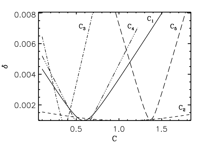
In their treatment, O03 use fiducial closure parameters in order to demonstrate the overall behavior of the model. He recommends the parameters to be calibrated by comparison with numerical simulations in order to obtain more accurate predictions. We have made an attempt to determine the dimensionless closure parameters that work for each value of in the range .
There are essentially two ways to approach the problem. The first is to take the time independent equations (16)–(25) and solve for using values of the traces and from the simulations. We call this method “backward modelling”. The problem with this method is that the Eqs. (16)–(25) are incomplete and do not set any constraints to the ratio . Consequently, it does not produce the correct solution to the time dependent equations (7) and (8). Therefore we also used the linear approximation described by Eqs. (26) and (27) to improve the fit.
The second way of determining is what we call “forward modelling”. The idea here is to seek such that the results of the time-dependent equations (7) and (8) yield the same individual stresses and the traces and as the numerical simulations. This time a universal is determined so that it predicts the stresses for all values . Once a reasonably good set of was found, the result was fine tuned further using the linear approximation given by Eqs. (26) and (27); see Figs. 4 and 5. From the Fig. 4 it can be seen that the best fit is obtained by fixing while keeping the other unchanged.
The final closure parameters are thus , , , and , corresponding to with , , , and . For these the relevant fit parameters in Eqs. (26) and (27) are and together with , , , , , and , , , , .


6 Discussion
In this study we set out to investigate the shear rate dependency of MRI-generated turbulent stresses. We have performed a series of local shearing box simulations with varying and measured the resulting turbulent stresses. We find that the turbulent stress ratio , and the total stress exhibit strong -dependency. The relation for the stress ratio by PCP06; see Eq. (6) predicts similar behaviour, but the ratio computed from the simulations is consistently 2-3 times larger than what their result indicates.
In order to further study the evolution of the MRI and the stresses we have attempted to reproduce them using the local closure model by O03. We first find a set such that the time-dependent equations give the same individual stresses and traces and . The linear approximation of Eqs. (26)–(27) is then used together with the time-independent equations to improve the fit. The O03 closure parameters that describe our numerical simulation results are found to be , , , and .
The closure model by O03 was thus found to predict our simulation generated turbulent stresses quite well. The model certainly offers a much-needed method for studying the evolution of turbulent stresses in the shearing sheet limit. However, additional constraints for and are needed in order to determine the closure parameters . The linear fitting approximation described in Eqs. (26) and (27) was devised to overcome this shortcoming.
Our results may also have some relevance in the galactic context, in which the MRI has been proposed to be responsible of the anomalous turbulent velocity dispersions found in the outer regions of some galaxies (e.g. Sellwood & Balbus 1999). On the other hand, the energy balance estimates from observations of NGC6949 (Beck 2004) indicate that magnetic energy could become dominant over the kinetic energy in the outer regions of this galaxy, so that the energy ratio –. According to our present results, in MRI-driven systems the magnetic energy clearly dominates over the kinetic energy for all , at the galactic value of for flat rotation curves we find the value , a number agreeing rather well with the observational estimates.
Acknowledgements.
It is a pleasure to thank an anonymous referee for a comprehensive report that lead to significant improvements in the manuscript. The authors also wish to express their gratitude to Nordita for their hospitality during the program ‘Turbulence and Dynamos.’ We acknowledge the Scientific Computing Ltd., Espoo, Finland, for granting CPU time in their supercomputers. This work was supported by the Academy of Finland through grants No. 112020 (AJL) and No. 121431 (PJK) and in part by the National Science Foundation under grant PHY05-51164 (AB).References
- [1] Abramowicz, M. Brandenburg, A., Lasota, J.-P.: 1996, MNRAS 281, L21
- [2] Armitage, P.J.: 1998, ApJ 501, 189
- [3] Balbus, S.A., Hawley, J.F.: 1991, ApJ 376, 214
- [4] Beck, R.: 2004, in How does the galaxy work?, ed. E.J. Alfaro, E. Pérez, & J. Franco, ASSL 315, 277
- [5] Blackman, E.G., Penna, R.F., Varniere, P.: 2008, New. A. 13, 244
- [6] Brandenburg, A., Nordlund, Å., Stein, R., Torkelsson U.:1995 ApJ 446, 741
- [7] Brandenburg, A., Dobler, W.: 2002, Comp. Phys. Comm. 147, 471
- [8] Garaud, P., Ogilvie, G.I.: 2005, J. Fluid Mech. 530, 145
- [9] Hawley, J.F., Gammie, C.F., Balbus, S.A.: 1995, ApJ 440, 742
- [10] Hawley, J.F., Gammie, C.F., Balbus, S.A.: 1996, ApJ 464, 690
- [11] Hawley, J.F., Balbus, S.A., Winters, W.F.: 1999, ApJ 518, 394
- [12] Hawley, J.F.: 2001, ApJ 554, 534
- [13] Haugen, N.E.L., Brandenburg, A.: 2006, Phys. Fluids 18, 075106
- [14] Johansen, A., Klahr, H.: 2005, ApJ 634, 1353
- [15] Kato S., Yoshizawa A.: 1995, Publ. Astron. Soc. Jap. 47, 629
- [16] Käpylä, P.J., Brandenburg, A.: 2008, A&A 488, 9
- [17] Lyra, W., Johansen, A., Klahr, H., Piskunov, N.: 2008, A&A 479, 883
- [18] Ogilvie, G.I.: 2003, MNRAS 340, 969 (O03)
- [19] Pessah, M.E., Chan, C.K., Psaltis, D.: 2006a, MNRAS 372, 183 (PCP06)
- [20] Pessah, M.E., Chan, C.K., Psaltis, D.: 2006b, PhRvL 97, 1103
- [21] Shakura N.I., Sunyaev R.A.: 1973, A&A 24, 337
- [22] Sellwood, J.A., & Balbus, S.A. 1999, ApJ 511, 660
- [23] Velikhov, E.P.: 1959, Sov. Phys. JETP 36, 1398
- [24] Wisdom, J., Tremaine, S.: 1988, AJ 95, 925