Bound on trace distance based on superfidelity

The trace distance is one of the most natural distance measures used in quantum-information theory [1, 2]. It is one of the main tools used in distinguishability theory and it is connected to the average success probability when distinguishing two states by a measurement [3, 5, 4]. It is also related to quantum fidelity, which provides the measure of similarity of two quantum states [1, 7, 6].

Both quantities are particularly important in quantum cryptography, since the security of quantum protocols relies on an ability to measure the distance between two quantum states [4]. The trace distance is also related to other properties of quantum states like the von Neumann entropy and relative entropy [1].

The main aim of this work is to provide a lower bound for the trace distance using measurable quantities. We use nonlinear functions of the form $\mathrm{tr}\rho_{i}\rho_{j},i,j=1,2$, where $\rho_{i}$ and $\rho_{j}$ are density matrices. For such forms there exist feasible schemes to measure them in an experiment without resorting to state tomography [8]. We give a lower bound based on the superfidelity introduced recently in [9]. Proof of this bound gives an answer to the conjecture stated by Mendonca et al. in [10].

Let us denote by $\Omega_{N}$ the space of density matrices acting on $N$-dimensional Hilbert space $\mathbb{C}^{N}$. For two density matrices $\rho_{1},\rho_{2}\in\Omega_{N}$ the trace distance is defined as

In the particular case of pure states we can use Bloch vectors $\rho_{1}=\vec{r}\cdot\vec{\sigma}$ and $\rho_{2}=\vec{s}\cdot\vec{\sigma}$. One can see that the trace distance between such states is equal to half of the Euclidean distance between the respective Bloch vectors

The trace distance can be bounded with the use of the fidelity [4, 1]

where the fidelity is defined as

The inequality (3) shows that $F$ and $D_{\mathrm{tr}}$ are closely related indicators of distinguishability.

The main result of this work is a lower bound for the trace distance, which we prove in the next section,

where $G$ is called the superfidelity, and was introduced in [9]. For $\rho_{1},\rho_{2}\in\Omega_{N}$ it is defined as

From the matrix analytic perspective the inequality (5) relates the trace norm on the space $\Omega_{N}$ to the Hilbert-Schmidt scalar product on $\Omega_{N}$.

For the sake of consistency we provide basic information about the superfidelity [9]. The most interesting feature of superfidelity is that it provides an upper bound for quantum fidelity [9]

The superfidelity also has properties which make it useful for quantifying the distance between quantum states. In particular we have: (1) Bounds: $0\leq G(\rho_{1},\rho_{2})\leq 1$. (2) Symmetry: $G(\rho_{1},\rho_{2})=G(\rho_{2},\rho_{1})$. (3) Unitary invariance: for any unitary operator $U$, we have $G(\rho_{1},\rho_{2})=G(U\rho_{1}U^{\dagger},U\rho_{2}U^{\dagger})$. (4) Concavity: $G(\rho_{1},\alpha\rho_{2}+(1-\alpha)\rho_{3})\geq\alpha G(\rho_{1},\rho_{2})+(1-\alpha)G(\rho_{1},\rho_{3})$ for any $\rho_{1},\rho_{2},\rho_{3}\in\Omega_{N}$ and $\alpha\in[0,1]$. (5) Supermultiplicativity: for $\rho_{1},\rho_{2},\rho_{3},\rho_{4}\in\Omega_{N}$ we have

Note that the superfidelity shares properties 1-4 with the fidelity. However, in contrast to the fidelity, superfidelity is not multiplicative, but supermultiplicative.

In [10] the authors showed that $G$ is jointly concave in its two arguments,

for $\alpha\in[0,1]$. Note that the property of joint concavity is obeyed by the square root of fidelity $\sqrt{F}(\rho_{1},\rho_{2})=\mathrm{tr}|\sqrt{\rho_{2}}\sqrt{\rho_{2}}|$, but not by the fidelity (4).

Fidelity can be used to define the metric $D_{B}(\rho_{1},\rho_{2})$ on the space $\Omega_{N}$ as

Unfortunately the analog of the Bures distance defined using the superfidelity

is not a metric [10], but the quantity

provides the metric on the space $\Omega_{N}$.

Finally one should note that the superfidelity is particularly convenient to use as the practical measure of similarity between quantum states. One of the main advantages of superfidelity is that it is possible to design feasible schemes to measure it in an experiment [9]. Also, from the computational point of view, calculation of the superfidelity is significantly less resource-consuming [10].

The properties of superfidelity listed above suggest that it would be convenient to use it instead of fidelity to draw conclusions about the distinguishability of quantum states. This section show how this can be done by relating the superfidelity and trace distance.

First we can observe that from the inequality

and since we have (3) we get that

Our main aim is to prove the following inequality, which provides tighter bound.

This inequality was first stated as a conjecture in [10], where it was verified numerically for small dimensions. Clearly it is motivated by the lower bound for trace distance provided by the inequality (3).

To prove the Theorem 1 we need the following lemma.

We subtract the right- from the left-side of (17) to get

because ${\rm 1\hskip-2.56073ptl}-\rho_{1}$ is positive semidefinite.

$\blacksquare$

$\blacksquare$

It is natural to consider the relation between the lower bounds in (3) and (5). It is clear that bound (5) is better than (3) whenever $G-\sqrt{F}\leq 0$.

In the one qubit case or if one of the states is pure the bound (5) is always better than (3). This follows from the equality between fidelity and superfidelity in these situations [9]. On the other hand the inequality (3) provides a better lower bound if the states $\rho_{1}$ and $\rho_{2}$ have orthogonal supports. In this case the fidelity between states vanishes, but the superfidelity is not necessarily equal to zero [9].

To get some feeling about the difference between the bound given by fidelity and the present bound we will consider the following families of states.

1. (i)

   The family $\rho_{\alpha}$ is defined as

   $$\rho_{\alpha}=\alpha|\psi\rangle\langle\psi|+(1-\alpha){\rm 1\hskip-2.56073ptl}/N,$$

   (27)

   where $|\psi\rangle\langle\psi|$ is a pure state and in our case we take $|\psi\rangle=|0\rangle\in\mathbb{C}^{N}$.

2. (ii)

   The family $\sigma_{\beta}\in\Omega_{8}$ is defined as

   $$\sigma_{\beta}=\beta|GHZ\rangle\langle GHZ|+(1-\beta){\rm 1\hskip-2.56073ptl}/N,$$

   (28)

   where $|GHZ\rangle=(1/\sqrt{2})(|000\rangle+|111\rangle)$.

3. (iii)

   The family $\tau_{\gamma}\in\Omega_{8}$ is defined as:

   $$\tau_{\gamma}=\gamma|010\rangle\langle 010|+(1-\gamma){\rm 1\hskip-2.56073ptl}/N.$$

   (29)

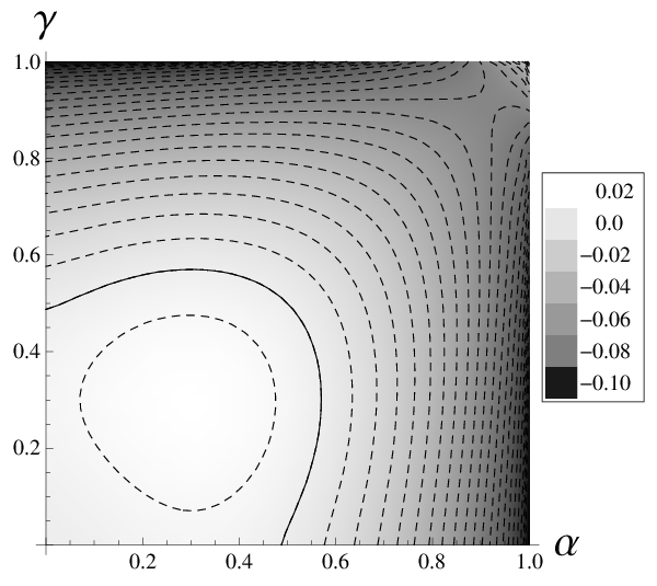
In Fig. 1 we consider the family $\rho_{\alpha}$ and calculate the difference $G(\rho_{\alpha},{\rm 1\hskip-2.56073ptl}/N)-\sqrt{F(\rho_{\alpha},{\rm 1\hskip-2.56073ptl}/N)}$. One can see that for small dimensions and states close to the pure state $|\psi\rangle\langle\psi|$ the superfidelity gives a much better approximation for the trace distance than the fidelity. For larger dimensions this is not the case, but nevertheless we can observe that still the superfidelity provides a better bound. This advantage is lost for states close to the maximally mixed state.

A similar situation can be observed in Fig. 2 where the difference between $G(\rho_{\alpha},\sigma_{\beta})$ and $\sqrt{F(\rho_{\alpha},\sigma_{\beta})}$ ($\rho_{\alpha},\sigma_{\beta}\in\Omega_{8}$) is presented. For this particular family the bound (5) is better than (3), but the difference vanishes for states close to the maximally mixed state.

Unfortunately, the bound (5) is not always tighter when compared with (3). Figure 3 shows the difference between $G(\rho_{\alpha},\tau_{\gamma})$ and $\sqrt{F(\rho_{\alpha},\tau_{\gamma})}$ ($\rho_{\alpha},\tau_{\gamma}\in\Omega_{8}$). As one can see for this family of states there are regions for which the bound (5) is better than (3) but in this case for highly mixed states (3) is better than (5).

We know that the probability of error for distinguishing two density matrices $\rho_{1},\rho_{2}\in\Omega_{N}$ is expressed by the trace distance as [1, 3]

Using the inequality (5) we can write

We have shown the relation between the superfidelity and trace distance, which is analogous to the relation with trace distance and fidelity. This shows that superfidelity can be used to conclude about the distinguishablity of states.

Experimental scheme proposed in [9] can be used to estimate superfidelity. Consequently it is possible to estimate experimentally provided lower bound for trace distance.

Our bound provides the relation between the trace distance and the overlap of two operators supplementary to inequality from [11, Th.1]. As such it provides neat mathematical tool which can be used in quantum information theory.