Space-Time Structure of Loop Quantum Black Hole
Abstract
In this paper we have improved the semiclassical analysis of loop quantum black hole (LQBH) in the conservative approach of constant polymeric parameter. In particular we have focused our attention on the space-time structure. We have introduced a very simple modification of the spherically symmetric Hamiltonian constraint in its holonomic version. The new quantum constraint reduces to the classical constraint when the polymeric parameter goes to zero. Using this modification we have obtained a large class of semiclassical solutions parametrized by a generic function . We have found that only a particular choice of this function reproduces the black hole solution with the correct asymptotic flat limit. In the semiclassical metric is regular and the Kretschmann invariant has a maximum peaked in . The radial position of the pick does not depend on the black hole mass and the polymeric parameter . The semiclassical solution is very similar to the Reissner-Nordström metric. We have constructed the Carter-Penrose diagrams explicitly, giving a causal description of the space-time and its maximal extension. The LQBH metric interpolates between two asymptotically regions, the region and the region. We have studied the thermodynamics of the semiclassical solution. The temperature, entropy and the evaporation process are regular and could be defined independently from the polymeric parameter . We have studied the particular metric when the polymeric parameter goes towards to zero. This metric is regular in and has only one event horizon in . The Kretschmann invariant maximum depends only on . The polymeric parameter does not play any role in the black hole singularity resolution. The thermodynamics is the same.
INTRODUCTION
Quantum gravity is the theory attempting to reconcile general relativity and quantum mechanics. In general relativity the space-time is dynamical, then it is not possible to study other interactions on a fixed background because the background itself is a dynamical field. The theory called “loop quantum gravity” (LQG) [1] is the most widespread nowadays. This is one of the non perturbative and background independent approaches to quantum gravity. LQG is a quantum geometric fundamental theory that reconciles general relativity and quantum mechanics at the Planck scale and we expect that this theory could resolve the classical singularity problems of General Relativity. Much progress has been done in this direction in the last years. In particular, the application of LQG technology to early universe in the context of minisuperspace models have solved the initial singularity problem [2], [3].
Black holes are another interesting place for testing the validity of LQG. In the past years applications of LQG ideas to the Kantowski-Sachs space-time [4] lead to some interesting results in this field. In particular, it has been showed [5] [6] that it is possible to solve the black hole singularity problem by using tools and ideas developed in full LQG. Other remarkable results have been obtained in the non homogeneous case [7].
There are also works of semiclassical nature which try to solve the black hole singularity problem [8],[9], [9]. In these papers the authors use an effective Hamiltonian constraint obtained replacing the Ashtekar connection with the holonomy and they solve the classical Hamilton equations of motion exactly or numerically. In this paper we try to improve the semiclassical analysis introducing a very simple modification to the holonomic version of the Hamiltonian constraint. The main result is that the minimum area [11] of full LQG is the fundamental ingredient to solve the black hole space-time singularity problem in . The sphere bounces on the minimum area of LQG and the singularity disappears. We show the Kretschmann invariant is regular in all space-time and the position of the maximum is independent on mass and on polymeric parameter introduced to define the holonomic version of the scalar constraint. The radial position of the curvature maximum depends only on and .
This paper is organized as follows. In the first section we recall the classical Schwarzschild solution in Ashtekar’s variables and we introduce a class of Hamiltonian constraints expressed in terms of holonomies that reduce to the classical one in the limit where the polymer parameter . We solve the Hamilton equations of motion obtaining the semiclassical black hole solution for a particular choice of the quantum constraint. In the third section we show the regularity of the solution by studying the Kretschmann operator and we write the solution in a very simple form similar to the Reissner-Nordström solution for a black hole with mass and charge. In section four we study the space-time structure and we construct the Carter-Penrose diagrams. In section five section we show the solution has a Schwarzschild core in . In section six we analyze the black hole thermodynamic calculating temperature, entropy and evaporation. In section seven we calculate the limit of the metric and we obtain a regular semiclassical solution with the same thermodynamic properties but with only one event horizon at the Schwarzschild radius. We analyze the causal space-time structure and construct the Carter-Penrose diagrams.
I Schwarzschild solution in Ashtekar variables
In this section we recall the classical Schwarzschild solution inside the event horizon [5] [6]. For the homogeneous but non isotropic Kantowski-Sachs space-time the Ashtekar’s variables [12] are
| (1) |
The components variables in the phase space have length dimension , , , . The Hamiltonian constraint is
| (2) |
Using the general relation ( is the metric on the spatial section) we obtain .
We restrict integration over to a finite interval and the Hamiltonian takes the form [6]
| (3) |
The rescaled variables are: , , , . The length dimensions of the new phase space variables are: , , , . From the symmetric reduced connection and density triad we can read the components variables in the phase space: , , with Poisson algebra , . We choose the gauge and the Hamiltonian constraint reduce to
| (4) |
The Hamilton equations of motion are
| (5) |
The solutions of equations (5) using the time parameter and redefining the integration constant (see the papers in [5] [6]) are
| (6) |
This is exactly the Schwarzschild solution inside and also outside the event horizon as we can verify passing to the metric form defined by ( contains the gravitational constant parameter ). The line element is
| (7) |
Introducing the solution (6) in (7) we obtain the Schwarzschild solution in all space-time except in where the classical curvature singularity is localized and except in where there is a coordinate singularity
| (8) |
where . To obtain the Schwarzschild metric we choose . In this way we fix the radial cell to have length and disappears from the metric. In the semiclassical LQBH metric does not disappears fixing . At this level we have not fixed but only the dimension of the radial cell. This is the correct choice to reproduce the Schwarzschild solution. We have defined the dimension of the cell in the direction to be obtaining the correct Schwarzschild metric in all space time, we will do the same choice for the semiclassical metric. With this choice will not disappears from the semiclassical metric and in particular from the solution. We will use the minimum area of the full theory to fix . For the semiclassical solution at the end of section (V) we will give also a possible physical interpretation of .
II A general class of Hamiltonian constrains
The correct dynamics of loop quantum gravity is the main problem of the theory. LQG is well defined at kinematical level but it is not clear what is the correct version of the Hamiltonian constraint, or more generically, in the covariant approach, what is the correct spin-foam model [13]. An empirical principle to construct the correct Hamiltonian constraint is to recall the correct semiclassical limit [14]. When we impose spherical symmetry and homogeneity, the connection and density triad assume the particular form given in (1). We can choose a large class of Hamiltonian constraints, expressed in terms of holonomies , which reduce to the same classical one (4) when the polymeric parameter goes towards to zero. We introduce a parametric function that labels the elements in the class of Hamiltonian constraints compatible with spherical symmetry and homogeneity. We call the constrain for the full theory and the constraint for the homogeneous spherical minisuperspace model. The reduction from the full theory to the minisuperspace model is
| (9) |
where the arrow represents the spherical symmetric reduction of the full loop quantum gravity hamiltonian constraint. To obtain the classical Hamiltonian constraint (4) in the limit we recall that the function satisfies the following condition
| (10) |
We are going to show that just one particular choice of gives the correct asymptotic flat limit for the Schwarzschild black hole. In fact the asymptotic selects the particular form of the function .
The classical Hamiltonian constraint can be written in the following form
| (11) |
where and ( is the extrinsic curvature, and ). The holonomies in the directions for a generic path are defined by
| (12) |
We define the field straight in terms of holonomies in the following way
| (13) |
it’s a simple exercise to verify that when (13) we obtain the classical field straight. The Hamiltonian constraint in terms of holonomies is
| (14) |
is the spatial section volume. We have introduced modifications depending on the function only in the field straight but this is sufficient to have a large class of semiclassical hamiltonian constraints compatible with spherical simmetry. The Hamiltonian constraint in (14) can be substantially simplified in the gauge
| (15) |
From (15) we obtain two independent sets of equations of motion on the phase space
| (16) |
Solving the first three equations and using the Hamiltonian constraint , with the time parametrization and imposing to have the Schwarzschild event horizon in , we obtain
| (17) |
where we have defined the quantities
| (18) |
Now we focus our attention on the term . The choice of this term and in particular the choice of the exponent will be crucial to have the correct flat asymptotic limit. The exponent is in the form and expanding in powers of the small parameter we obtain at large distance () (we remember that outside the event horizon the coordinate t plays the rule of spatial radial coordinate). It is straightforward to see that exists only one possible way to obtain the correct asymptotic limit and it is given by the choice . In other words we can say that any function diverges logarithmically for small and large distance ().
Let as take . In force of the correct large distance limit and in force also of the regularity of the curvature invariant in all space time, we will extend the solution outside the event horizons with the redefinition . I will come back to this extension in the next section.
A crucial difference with the classical Schwarzschild solution is that has a minimum in , and . The solution has a spacetime structure very similar to the Reissner-Nordström metric and presents an inner horizon in
| (19) |
For , . We observe that the inside horizon position (we recall is the Barbero-Immirzi parameter).

Now we study the trajectory in the plane and we compare the result with the Schwarzschild solution. In Fig.1 we have a parametric plot of ; we can follow the trajectory from where the classical (dashed trajectory) and the semiclassical (continuum trajectory) solution are very close. For , and (this point corresponds to the Schwarzschild radius). From this point decreasing we reach a minimum value for . From , starts to grow again until , this point corresponds to a new horizon in localized. In the time interval , grows together with and as it is very clear from the picture the solution approach the second specular black hole for . In particular we have a second asymptotic region for .
Metric form of the solution.
In this section we write the solution in the metric form and we extend that to the all space-time. We recall the Kantowski-Sachs metric is . The metric components are related to the connection variables by
| (20) |
We have introduced by a coordinate transformation ,
| (21) |
This coordinate transformation is useful to obtain the Minkowski metric in the limit . The explicit form of the lapse function in terms of the coordinate is
| (22) |
Using the second relation in (20) we can obtain the metric component,
| (23) |
The function corresponds to given in (17). The metric obtained has the correct asymptotic limit for and in fact , , . The semiclassical metric goes to a flat limit also for . We can say that LQBH interpolates between two asymptotic flat region of the space-time. The metric obtained in this paper has the correct flat asymptotic limit for and reproduce the Minkowski metric for . Both those limit are not satisfied in the work [8]. The small modification introduced in the holonomy form of the Hamiltonian is necessary for those two fundamental consistency limit.
III LQBH in all space-time
In this section we extend the (metric) semiclassical solution obtained obtained in the previous section to all space-time. As explained in the previous subsection the metric solution has the correct flat limit for and goes to Minkowski for . Now we shaw that the Kretschmann scalar is regular in all space-time. In terms of , and the Kretschmann scalar is
| (24) |
In Fig.2 is plotted a graph of , it is regular in all space-time and the large behavior is the classical singular scalar .

What about ? Now we fix the parameter using the full theory (LQG). In particular we choose in such way the position of the Kretschmann invariant maximum is independent of the black hole mass. This means the sphere bounces on a minimum radius that is independent from the mass of the black hole and from and depends only on . We consider the solution and we impose the minimum area of the sphere to be equal to the minimum gap area of loop quantum gravity . With the choice we obtain a significative physical result. We have not impose to have a minimum in but we have just impose that the minimum of is the minimum area of the full theory. The minimum area of the two sphere is a result and not a request. We observe that this choice of fixes the absolute maximum and relative minimum of to be independent of the mass as this is manifest from the plot in Fig.3.
We want to provide an argument to support the choice . In the paper [15] it is shown the phase space is parametrized by and the conjugated momentum and it is shown that are both constants of motion (in our notation ). As usual in elementary quantum mechanics to derive the Heisenberg uncertainty relation, we can introduce the state , where and are the mass and momentum operators and . From the positive norm we have the discriminant, of second order in , is negative or zero. The condition on the discriminant gives . Introducing the commutator we obtain . We can calculate on semiclassical gaussian states,
| (25) |
and the result is (for ). Using the Heisenberg uncertainty relation we determine . If we identify we obtain , which is exactly for , and . We have introduced explicitly all the coefficients but the main result is . However the presented here is just an argument and not a proof.
At the end of section (V) we will give a physical interpretation of .

We now want underline the similarity between the equation of motion for and the Friedmann equation of loop quantum cosmology. We can write the differential equation for in the following form
| (26) |
From this equation is manifest that bounces on the value . This is quite similar to the loop quantum cosmology bounce [16].
As it is evident from Fig.4 the maximum of the Kretschmann invariant is independent of the mass and it is in localized. At this point we redefine the variables (with the subsequent identification ) and the metric components to bring the solution in the standard Schwarzschild form
| (27) |
Schematically the properties of the metric are the following,
| (28) |
We consider the property (28) sufficient to extend the solution in all space-time.


The solution is summarized in the following table (in the table we have not fixed the parameter ).
We have said in the previous section the metric solution has two event horizons. An event horizon is defined by a null surface . The surface is a null surface if the normal is a null vector or satisfied the condition . The last identity says that the vector is on the surface itself, in fact and . The norm of the vector is given by
| (29) |
In our case (29) reduces to
| (30) |
and this equation is satisfied where and if the surface is independent from , . The points where are and .
We can write the metric in another form which is more similar to the Reissner-Nordström space-time. The metric can be written in the following form
| (31) |
If we develop the metric (31) by the parameter and the minimum area at the zero order we obtain the Schwarzschild solution: , and . We have correction to the metric from the polymer parameter and also from the minimum area .
To check the semiclassical limit we calculate the perturbative expansion of the curvature invariant for small and and we obtain a divergent quantity in at any order of the development. The regularity of is a non perturbative result, in fact for small values of the radial coordinate , diverges for . (For the semiclassical solution the trace of the Ricci tensor () is not identically zero as for the Schwarzschild solution. We have calculated also this operator and we have obtained a regular quantity in ).


We conclude this section showing the independence of the pick position of Kretschmann invariant from the polymeric parameter . We have plotted the invariant and we have obtained the result in Fig.(7).

From the picture is evident the position of the Kretschmann invariant maximum is independent from .
Corrections to the Newtonian potential.
In this paper we are interested to to singularity problem in black hole physics and not to the Post-Newtonian approximation, however we want give the fist correction to the gravitational potential. The gravitational potential is related to the metric by . Developing the component of the metric in power of to the order , for fixed values of the parameter and the minimal gap area , we obtain the potential
where is defined in (18).
IV Causal structure and Carter-Penrose diagram
In this section we construct the Carter-Penrose diagrams [17] for the semiclassical metric (31). To obtain the diagrams we will do many coordinate changing and we enumerate them from one to eight.
1) We can put the metric (31) in the form introducing the tortoise coordinate defined by :
| (33) |
2) The second coordinate set to use is , where and . The metric becomes .
3) The singularity on the event horizon disappearances using the coordinates ( defined by , , where
| (34) |
We introduce also the parametric function
| (35) |
Note that and . In those coordinates the metric is
| (36) |
where we have introduced the function which is defined implicitly in terms of and .
4) Using coordinate () defined by , , the metric (36) assumes the conformally flat form . In those coordinates the trajectories of constant -coordinate are
| (37) |
The event horizons and are localized in
| (38) |
5) A first Carter-Penrose diagram for the region can be construct using coordinates () defined by , and , . The event horizon is localized in or . The event horizon is localized in or: for , for . The other asymptotic regions are: (), (), (), (). The Carter-Penrose diagram for this region is given in the picture on the left in Fig.(8).


6) In the coordinates introduced above, the metric (31) is not regular in . To remove the singularity in we introduce the coordinates () defined by , . In those coordinates the metric is
| (39) |
where . Now the metric is regular in but singular in .
7) As in the region we introduce coordinates () in terms of which . The -constant trajectories are defined by the curves
| (40) |
In particular the horizons and the point are defined by the curves
| (41) |
8) In coordinate () defined by , . The event horizon is localized in or , The event horizon is localized in or: for , for . The other asymptotic regions are defined by : for and for . The Carter-Penrose diagram for this region is the picture on the right in Fig.(8).
Now we are going to show that any massive particle could not fall in in a finite proper time. We consider the radial geodesic equation for a massive point particle
| (42) |
where “” is the proper time derivative and is the point particle energy. If the particle falls from the infinity with zero initial radial velocity the energy is . We can write (42) in a more familiar form
| (43) |
A plot of is in Fig.(9). For , then any particle with could not arrive in . If the particle energy is , the geodesic equation for is and integrating or .


We can compose the diagrams in Fig.(8) to obtain a maximal extension similar to the Reissner-Nordström one, the result is represented in Fig.(10).

V Asymptotic Schwarzschild core near
In this section we study the limit of the metric (31). If we develop the metric very closed to the point we obtain :
| (44) |
The parametric functions are
| (45) |
We consider the coordinate changing . The point is mapped in the point . The metric in the new coordinates is
| (46) |
where and are functions of ,
| (47) |
For small we obtain and (46) converges to the Schwarzschild metric of mass . We can conclude the space-time near the point is described by an effective Schwarzschild metric of mass in the large distance limit . An observer in the asymptotic region experiments a Schwarzschild metric of mass .
We now want give a possible physical interpretation of . If we reintroduce in the core mass defined above we obtain , then we can interpret as the mass of the black hole as it is seen from an observer in . In [9] the authors interpret as the mass of a second black hole, in our analysis instead seems to be the mass of the black hole but from the point of view of an observer in the asymptotic region .
VI LQBH termodynamics
In this section we study the termodynamics of the LQBH [19]. The form of the metric calculated in the previous section has the general form
| (48) |
where the functions , and depend on the mass parameter and are the components of the metric (31). We can introduce the null coordinate to express the metric (48) in the Bardeen form. The null coordinate is defined by the relation , where and the differential is . In the new coordinate the metric is
| (49) |
We can interpret our black hole solution has been generated by an effective matter fluid that simulates the loop quantum gravity corrections (in analogy with the paper [19]). The effective gravity-matter system satisfies by definition of the Einstein equation , where is the effective energy tensor. The stress energy tensor for a perfect fluid compatible with the space-time symmetries is and in terms of the Einstein tensor the components are , and . The semiclassical metric to zero order in and is the classical Schwarzschild solution () that satisfies .
VI.1 Temperature
In this paragraph we calculate the temperature for the quantum black hole solution and analyze the evaporation process. The Bekenstein-Hawking temperature is given in terms of the surface gravity by , the surface gravity is defined by where is a timelike Killing vector and is the connection compatibles with the metric of (48). Using the semiclassical metric we can calculate the surface gravity in obtaining and then the temperature,
| (50) |
The temperature (50) coincides with the Hawking temperature in the large mass limit. In Fig.11 we have a plot of the temperature as a function of the black hole mass .

The dashed trajectory corresponds to the Hawking temperature and the continuum trajectory corresponds to the semiclassical one. There is a substantial difference for small values of the mass, in fact the semiclassical temperature tends to zero and does not diverge for . The temperature is maximum for and . Also this result, as for the curvature invariant, is a quantum gravity effect, in fact depends only on the Planck area . If we calculate the limit in and we obtain two physical quantities which are independent of ,
| (51) |
VI.2 Entropy
In this section we calculate the entropy for the LQBH metric. By definition the entropy as function of the ADM energy is . Calculating this integral for the LQBH we find
| (52) |
We can express the entropy in terms of the event horizon area. The event horizon area (in ) is
| (53) |
Inverting (53) for and introducing the result in (52) we obtain
| (54) |
A plot of the entropy is in Fig.12. The first plot represents entropy as a function of the event horizon area . The second plot in Fig.12 represents the event horizon area as function of . The semiclassical area has a minimum value in for . As for the temperature also for the entropy we can calculate the limit and we obtain a regular quantity which depends on the event horizon area, on the Planck area but it is independent from ,
| (55) |
In the limit , .
We want underline the parameter does not play any regularization rule in the observable quantities , , and in the evaporation process that we will study in the following section. We obtain finite quantities taking the limit . This is an important prediction of the model.


VI.3 The evaporation process.
In this section we focus our attention on the evaporation process of the black hole mass and in particular in the energy flux from the hole. First of all the luminosity can be estimated using the Stefan law and it is given by , where (for a single massless field with two degree of freedom) , is the event horizon area and is the temperature calculated in the previous section. At the first order in the luminosity the metric (49) which incorporates the decreasing mass as function of the null coordinate is also a solution but with a new effective stress energy tensor as underlined previously. Introducing the results (50) and (53) of the previous paragraphs in the luminosity we obtain
| (56) |
Using (56) we can solve the fist order differential equation
| (57) |
to obtain the mass function . The result of integration with initial condition is
| (58) |
where , , , , . From the solution (58) we see the mass evaporate in an infinite time. Also in (58) we can take the limit obtaining a regular quantity independent from . In the limit equation (58) becomes
| (59) |
We can take the limit obtaining . Inverting this equation for small we obtain: .
VII The metric for
We have shown in the previous section that same physical observable can be defined independently from the polymeric parameter . This result suggest to calculate the limit of the semiclassical metric (31) for . We will obtain a regular metric and we will study its space-time structure. In the quantum theory we can not take the limit because we haven’t weakly continuity in the polymeric parameter . However the LQBH’metric (31) is very close to the Reissner-Nordström metric which is not stable and this suggest that also (31) could be not stable when we consider non homogeneities [20]. If it is the case then the horizon disappearances or in other words by (19), . Another motivation to calculate and to study this extreme limit of the metric is to show that the polymeric parameter does not play any rule in the singularity problem reslution. For the () plot is given in Fig.13.

We redefine the metric of section (31) introducing an explicit dependence from (the redefinition is: ). The new metric is mathematically defined by
| (60) |
The result of this limit gives the following very simple metric which is independent from the polymeric parameter ,
| (61) |
This metric has an event horizon in and this is in accord with the solution for general values of , in fact . The question now is to see if the solution is regular in all space-time and in particular in . We can calculate the Kretschmann invariant and we obtain
| (62) |
The invariant (62) is regular in all space-time and in particular in . For we find and for we have that shows the non perturbative character of the singularity resolution. From the second picture in Fig.(16) is evident the -coordinate of the pick of the curvature invariant is independent from the black hole mass.


What about temperature, entropy and the evaporation process? We calculate the surface gravity for the metric (61) and we obtain
| (63) |
This result is exactly the same quantity obtained in section (VI) but with . From this point the analysis is the same of section (VI): temperature, entropy and evaporation are the same of (51), (55), (58).
Causal structure and Carter-Penrose diagrams
In this section we construct the Carter-Penrose diagrams for the metric obtained taking the limit . To obtain the diagrams we must do many coordinate changing and we enumerate them from one to five.
1) First of all we calculate the tortoise coordinate for the metric (61) defined by ,
| (64) |
The coordinate (64) reduces to the Schwarzschild tortoise coordinate for . On the other side for , . Using coordinate the metric is
| (65) |
where is implicitly define by (64) (from now on we will not write the sphere part of the metric).
2) Now we write the metric in coordinate defined by and . The metric becomes
| (66) |
where is defined implicitly in terms of .
3) We can do another coordinate changing which leaves the two space conformally invariant. The news coordinate are defined by and . The metric is
| (67) |
4) We introduce the new coordinates defined by and . The metric is
| (68) |
All the coordinates in the conformal factor are implicitly defined in terms of .
At this point we choose explicitly the functions and to eliminate the singularity in . Following the analysis of the Schwarzschild case we take and , where . This is the correct coordinate changing also in our case to eliminate the coordinate singularity on the event horizon. We define the function that in terms of the radial coordinate becomes
| (69) |
The metric is regular on the event horizon. In the coordinates the event horizon and the point are localized respectively in
| (70) |
5) We conclude writing the metric in the coordinates defined by and . The event horizon is defined by the curve and then by the . From (70) the point is defined by the curve and or by the segments (), (). The other sectors are: (), (), (). The Carter-Penrose diagram of the regular space-time is represented in Fig.(16). The maximal space-time extension is represented in Fig.(17), the diagram can be infinitely extended in the four directions.
We now show that a massive particle arrives in in a finite proper time. The radial geodesic equation is ( is the proper time, the particle energy) and for reduces to . The solution is and the proper time to fall in starting from is: . Any massive particle falls in in a finite proper-time interval.
To conclude the analysis we extend the radial coordinate to negative values. The surface is a null surface as can be shown following the analysis in (III) (in particular ). We can extend the radial coordinate to negative values because the space-time is singularity free. The metric is asymptotically flat for and at the order takes the form
Because we have not event horizons in the negative region. The metric (61) is regular in all space-time .

The Carter-Penrose diagrams are in Fig.(18).


We can obtain the same results of this section in another equivalent way. Essentially what we have done in this section is to show that to solve the black hole singularity problem at semiclassical level it is sufficient to replace the component with the holonomy without to replace the component with the relative holonomy. In fact the solution (61) can be obtained directly from the semi-quantum Hamiltonian constraint
| (72) |
The scalar constraint (72) is classic in the sector but quantum in the sector ( and ). The constraint introduced in (14) is not the more general. We can introduce two different polymeric parameter and respectively in the directions and obtaining the constraint
| (73) |
and . The scalar constraint (72) is obtained taking the limit
| (74) |
The main result is that the singularity problem is solved by a bounce of the two sphere on a minimal area . The parameter does not play any role in the singularity problem resolution. This is evident from the Kretschmann invariant (62) which is independent from . The parameter is related to the position of the inner horizon and for the horizon disappearances.
CONCLUSIONS & DISCUSSION
In this paper we have introduced a simple modification of the holonomic Hamiltonian constraint which gives the metric with the correct semiclassical asymptotic flat limit when the Hamilton equations of motion are solved. We recall here the LQBH’s metric
| (75) |
We have shown the LQBH’s metric (75) has the following properties
- 1.
,
- 2.
,
- 3.
,
- 4.
,
- 5.
.
In particular (see point 5.) the position where the Kretschmann invariant operator is maximum is independent from the black hole mass and from the polymeric parameter . The metric has two event horizons that we have defined and ; is the Schwarzschild event horizon and is an inside horizon. The solution has many similarities with the Reissner-Nordström metric but without curvature singularities. In particular the region corresponds to another asymptotically flat region. Any massive particle can not arrive in this region in a finite proper time. A careful analysis shows the metric has a Schwarzschild core in of mass .
We have calculated the limit of the LQBH metric obtaining another metric regular in . This solution can be also obtained from (75) taking the limit or more simple and . The result is
| (76) |
This metric could be see as a solution of the Hamilton equation of motion for the semi-quantum scalar constraint (72).
Our analysis shows that the singularity problem is solved by a bounce of the sphere on a minimum area . This happens for both the metrics obtained in this paper, the first one of Reissner-Nordström type (75) and the second one of Schwarzschild type (76). The parameter does not play any rule in the singularity resolution problem. The solution (76) has all the good properties of (75) and in particular it is singularity free. This metric has an event horizon in and the thermodynamics is exactly the same of (75). When we consider the maximal extension to we find a second internal event horizon in .
We have studied the black hole thermodynamics : temperature, entropy and the evaporation process. The main results are:
- 1.
The temperature is regular for and reduces to the Bekenstein-Hawking temperature for large values of the mass Bekenstein-Hawking
(77) - 2.
The black hole entropy in terms of the event horizon area and the LQG minimum area eigenvalue is
(78) - 3.
The evaporation process needs an infinite time in our semiclassical analysis but the difference with the classical result is evident only at the Planck scale. In this extreme energy conditions it is necessary a complete quantum gravity analysis that can implies a complete evaporation [18].
We have shown it is possible to take the limit in , and the evaporation process equation obtaining regular quantities independent of the polymeric parameter . The result of the limit are physical quantities that depend only on the Planck area and not on the polymeric parameter.
We want to conclude the discussion with a stimulating observation. In this paper we have calculated the temperature (77) that in general we can see as a relation between temperature, mass and the minimum area . If we solve (77) for the minimum area we obtain the universal critical behavior . The critical exponent is independent from the mass and from the particular choice of the Hamiltonian constraint modification. The critical temperature is the classical Hawking temperature [21].
Some open problems.
In this paper we have fixed the parameter (which comes from the integration of the Hamilton equations of motion) introducing the minimum area (of the full theory) in the metric solution. In this way we have obtained a bounce of the sphere on the minimum area . A priori it is not obvious how to obtain the same bounce at the quantum level. However solving the quantum constraint we think we will obtain a bounce on a minimum area . The QEE contains only dimensionless quantities, the eigenvalues of the operators , and the polymeric parameter . When we reintroduce the length dimensions in the QEE we have , , then in the quantum evolution will play the rule played by in the semiclassical analysis and we will have a quantum bounce of the wave function on . This is manifest in the effective Wheeler-DeWitt equation obtained from the QEE in the limit , [6] where appears explicitly,
| (79) |
However the quantum evolution of a coherent Schwarzschild state is an open problem.
A problem related to the previous one is that we have fixed the integration in the direction to a cell of finite volume and this can imply a non scale invariant resolution of the singularity problem under a rescaling [23].
Another problem can be related to the entropy calculation. In fact we obtain a regular entropy but we do not obtain the usual logarithmic correction. We think it is possible to solve this problem with a simple modification of the holonomic version of the Hamiltonian constraint or taking into account the possibility that quantum properties of the background space-time alter geometry near the horizon [24].
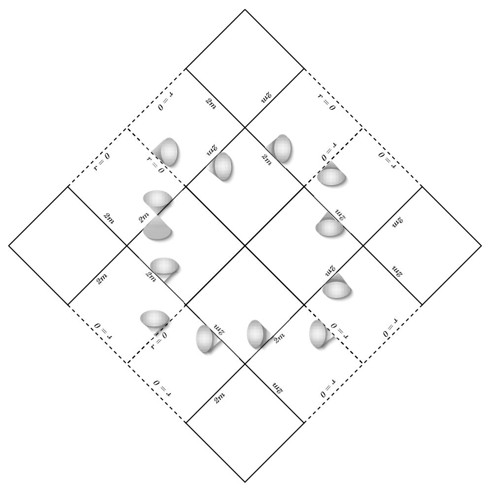
Other problems could be related to the maximal extension of the space-time. If we observe carefully the diagram in Fig.17 we can see that close time-like curve (CTC) are possible. This is manifest in the Fig.19 where a null CTC is represented by a close black curve. In the second diagram of Fig.19 we have represented the light cones along a CTC curve. We can have CTCs also with just one diagram if we identify the upper and lower extremes of the diagram (18).

Acknowledgements
We are grateful also to Parampreet Singh, Michele Arzano and Eugenio Bianchi for many important and clarifying discussions.
References
- [1] Carlo Rovelli, Quantum Gravity, (Cambridge University Press, Cambridge, 2004); A. Ashtekar, Background independent quantum gravity: A Status report, Class. Quant. Grav. 21, R53 (2004), gr-qc/0404018; T. Thiemann, Loop quantum gravity: an inside view, hep-th/0608210; T. Thiemann, Introduction to Modern Canonical Quantum General Relativity, gr -qc/0110034; Lectures on Loop Quantum Gravity, Lect. Notes Phys. 631, 41-135 (2003), gr-qc/0210094
- [2] Martin Bojowald, Loop quantum cosmology, Living Rev. Rel. 8:11, 2005, gr-qc/0601085; Martin Bojowald, Absence of singularity in loop quantum cosmology Phys. Rev. Lett. 86:5227-5230, 2001. e-Print: gr-qc/0102069
- [3] A. Ashtekar, M. Bojowald and J. Lewandowski, Mathematica structure of loop quantum cosmology, Adv. Theor. Math. Phys. 7 (2003) 233-268, gr-qc/0304074 Abhay Ashtekar , Tomasz Pawlowski, Parampreet Singh, Kevin Vandersloot, Loop quantum cosmology of k=1 FRW models, Phys. Rev. D75 (2007) 024035, gr-qc/0612104; Abhay Ashtekar, Tomasz Pawlowski, Parampreet Singh, Quantum Nature of the Big Bang: Improved dynamics, Phys. Rev. D74 (2006) 084003, gr-qc/0607039; Abhay Ashtekar, Tomasz Pawlowski, Parampreet Singh, Quantum Nature of the Big Bang: An Analytical and Numerical Investigation. I, Phys.Rev.D73 (2006) 124038, gr-qc/0604013
- [4] R. Kantowski and R. K. Sachs, J. Math. Phys. 7 (3) (1966); Luca Bombelli & R. J. Torrence Perfect fluids and Ashtekar variables, with application to Kantowski-Sachs models, Class. Quant. Grav. 7 (1990) 1747-1745
- [5] Leonardo Modesto, Disappearance of the black hole singularity in loop quantum gravity, Phys. Rev. D 70 (2004) 124009, gr-qc/0407097; Leonardo Modesto, The kantowski-Sachs space-time in loop quantum gravity, International Int. J. Theor. Phys. 45 (2006) 2235-2246, gr-qc/0411032; Leonardo Modesto, Loop quantum gravity and black hole singularity, proceedings of 17th SIGRAV Conference, Turin, Italy, 4-7 Sep 2006, hep-th/0701239; Leonardo Modesto, Gravitational collapse in loop quantum gravity, Int. J. Theor. Phys.47 (2008) 357-373, gr-qc/0610074; Leonardo Modesto, Quantum gravitational collapse, gr-qc/0504043
- [6] A. Ashtekar and M. Bojowald, Quantum geometry and Schwarzschild singularity Class. Quant. Grav. 23 (2006) 391-411, gr-qc/0509075; Leonardo Modesto, Loop quantum black hole, Class. Quant. Grav. 23 (2006) 5587-5602, gr-qc/0509078
- [7] Rodolfo Gambini, Jorge Pullin, Black holes in loop quantum gravity: The Complete space-time, Phys. Rev. Lett.101:161301, 2008, arXiv:0805.1187; Miguel Campiglia, Rodolfo Gambini, Jorge Pullin, Loop quantization of spherically symmetric midi-superspaces : the interior problem, AIP Conf. Proc. 977:52-63, 2008, arXiv:0712.0817; Miguel Campiglia, Rodolfo Gambini, Jorge Pullin, Loop quantization of spherically symmetric midi-superspaces Class. Quant. Grav. 24:3649-3672, 2007, gr-qc/0703135
- [8] Leonardo Modesto, Black hole interior from loop quantum gravity, gr-qc/06011043; Leonardo Modesto, Evaporating loop quantum black hole, gr-qc/0612084
- [9] ChristianG. Bohmer, KevinVandersloot, Loop quantum dynamics of the Schwarzschild Interior, arXiv:0709.2129
- [10] Dah-Wei Chiou, Phenomenological Loop Quantum Geometry of the Schwarzschild Black Hole, arXiv:0807.0665
- [11] C. Rovelli and L. Smolin, Loop Space Representation Of Quantum General Relativity, Nucl. Phys. B 331 (1990) 80; C. Rovelli and L. Smolin, Discreteness of area and volume in quantum gravity, Nucl. Phys. B 442 (1995) 593; Eugenio Bianchi, The Length operator in Loop Quantum Gravity, Nucl. Phys. B 807 (2009) 591-624, arXiv:0806.4710
- [12] Abhay Ashtekar, New Hamiltonian formulation of general relativity, Phys. Rev. D 36 1587-1602
- [13] Florian Conrady, Laurent Freidel, Path integral representation of spin foam models of 4d gravity, arXiv:0806.4640; Jonathan Engle, Etera Livine, Roberto Pereira, Carlo Rovelli, LQG vertex with finite Immirzi parameter, Nucl. Phys. B799 (2008) 136-149, arXiv:0711.0146; Jonathan Engle, Roberto Pereira, Carlo Rovelli, Flipped spinfoam vertex and loop gravity Nucl. Phys. B798 (2008) 251-290, arXiv:0708.1236; Jonathan Engle, Roberto Pereira, Carlo Rovelli, The Loop-quantum-gravity vertex-amplitude, Phys. Rev. Lett. 99 (2007) 161301, arXiv:0705.2388
- [14] Florian Conrady, Laurent Freidel, On the semiclassical limit of 4d spin foam models, arXiv:0809.2280; Emanuele Alesci, Carlo Rovelli, The Complete LQG propagator I. Difficulties with the Barrett-Crane vertex, Phys. Rev. D76 (2007) 104012, arXiv:0708.0883; Simone Speziale, Background-free propagation in loop quantum gravity arXiv:0810.1978; Eugenio Bianchi, Leonardo Modesto, Carlo Rovelli, Simone Speziale Graviton propagator in loop quantum gravity, Class. Quant. Grav. 23 (2006) 6989-7028, gr-qc/0604044; Leonardo Modesto, Carlo Rovelli Particle scattering in loop quantum gravity in Phys. Rev. Lett. 95 (2005) 191301, gr-qc/0502036; Eugenio Bianchi, Leonardo Modesto, The Perturbative Regge-calculus regime of loop quantum gravity, Nucl. Phys. B 796 (2008) 581-621, arXiv:0709.2051; Eugenio Bianchi, Alejandro Satz, Semiclassical regime of Regge calculus and spin foams, arXiv:0808.1107
- [15] Karel V. Kuchar, Geometrodynamics of Schwarzschild Black Hole, Phys. Rev. D50 (19994) 3961-3981, gr-qc/9403003; T. Thiemann, Reduced models for quantum gravity, Lect. Notes Phys. 434 (1994) 289-318, gr-qc/9910010; H.A. Kastrup, T. Thiemann, Spherically symmetric gravity as a completely integrable system, Nucl. Phys. B 425 (1994) 665-686, e-Print: gr-qc/9401032; T. Thiemann, H.A. Kastrup, Canonical quantization of spherically symmetric gravity in Ashtekar’s selfdual representation Nucl. Phys. B 399 (1993) 211-258, gr-qc/9310012
- [16] Abhay Ashtekar, Tomasz Pawlowski, Parampreet Singh, Quantum Nature of the Big Bang: An Analytical and Numerical Investigation. I, Phys.Rev.D73 (2006) 124038, gr-qc/0604013
- [17] Alessandro Fabbri and Jose Navarro-Salas, Modeling Black Hole Evaporation, Imperial College Press (2005)
- [18] Abhay Ashtekar & Martin Bojowald, Black hole evaporation : A paradigm Class. Quant. Grav. 22 (2005) 3349-3362, gr-qc/0504029
- [19] Alfio Bonanno, Martin Reuter, Renormalization group improved black hole space-times, Phys. Rev. D 62 (2000) 043008, hep-th/0002196; Alfio Bonanno, Martin Reuter Spacetime structure of an evaporating black hole in quantum gravity, Phys. Rev. D 73 (2006) 083005, hep-th/0602159; Yun Soo Myung, Yong-Wan Kim, Young-Jai Park, Thermodynamics of regular black hole, arXiv:0708.3145; Yun Soo Myung, Yong-Wan Kim, Young-Jai Park, Quantum Cooling Evaporation Process in Regular Black Holes Phys. Lett. B (2007) 656:221-225, gr-qc/0702145; Piero Nicolini, Noncommutative Black Holes, The Final Appeal To Quantum Gravity: A Review, arXiv:0807.1939
- [20] Michael Simpson and Roger Penrose, Internal instability in Reissner-Nordström black hole, Int. J. Theor. Phys. 7 (1973) 183-197
- [21] Danile Oriti, Group field theory as the microscopic description of the quantum spacetime fluid: A New perspective on the continuum in quantum gravity arXiv:0710.3276
- [22] Luca Bombelli & R. J. Torrence Perfect fluids and Ashtekar variables, with application to Kantowski-Sachs models Class. Quant. Grav. 7 (1990) 1747-1745
- [23] Alejandro Corichi and Parampreet Singh, Is loop quantization in cosmology unique?, Phys. Rev. D78 (2008) 024034, e-Print: arXiv:0805.0136
- [24] Michele Arzano, Black hole entropy, log corrections and quantum ergosphere Phys.Lett.B634 (2006) 536-540, gr-qc/0512071; Michele Arzano, A.J.M. Medved, Elias C. Vagenas, Hawking radiation as tunneling through the quantum horizon JHEP 0509 (2005) 037, hep-th/0505266