Optimized single-qubit gates for Josephson phase qubits
Abstract
In a Josephson phase qubit the coherent manipulations of the computational states are achieved by modulating an applied ac current, typically in the microwave range. In this work we show that it is possible to find optimal modulations of the bias current to achieve high-fidelity gates. We apply quantum optimal control theory to determine the form of the pulses and study in details the case of a NOT-gate. To test the efficiency of the optimized pulses in an experimental setup, we also address the effect of possible imperfections in the pulses shapes, the role of off-resonance elements in the Hamiltonian, and the effect of capacitive interaction with a second qubit.
pacs
85.25.Cp, 03.67.Lx, 02.30.YyI Introduction
Over the past decades, together with the development of the theory of quantum information [1] there has been an increasing effort to find those physical systems where quantum information processing could be implemented. Among the many different proposals, devices based on superconducting Josephson junctions are promising candidates in the solid state realm (see the reviews in Ref. 2, 3, 4, 5). Josephson qubits can be categorized into three main classes: Charge, phase and flux qubits, depending on which dynamical variable is most well defined and consequently which basis states are used as computational states and .
Phase qubits [6, 7, 8], subject of the present investigation, in their simplest configuration can be realized with a single current biased Josephson junction. For bias lower that the critical current, the two lowest eigenstates of the system form the computational space. The application of a current pulse, with frequency which is in resonance with the transition frequency of the two logical states, typically in the microwave range, allows to perform all desired single bit operations. Recent experiments [10, 9] have realized both single-bit and two-bit gates in capacitive coupled phase qubits. In the experiments conducted so far, motivated by similar approach in NMR, the amplitude of the microwave current used to perform the qubit manipulation has a Gaussian shape [9, 11]. The importance of achieving fast quantum gates with high fidelity rises the question whether there are modulations, other than Gaussian, which lead to higher fidelities. Indeed, Gaussian pulses act better when their duration time is longer [11], therefore the search for modulations which result in high fidelity gates, even when the duration time of the pulse is short, seems to be necessary. Some theoretical work has already been done in this direction to examine the efficiency of different modulations [11]. In the present paper we follow a different approach as compared to Ref. 11 and show that by employing the quantum optimal control theory [12, 13, 14, 15], we can further improve the (theoretical) bounds on the error of gate operations.
Quantum optimal control has been already applied to optimize quantum manipulation of Josephson nanocircuits in the charge limit [16, 17, 18]. Here we want to test this method in the opposite regime of phase qubit [19] and see whether it is possible to find optimal modulations of microwave pulses, with different duration times, which give very good fidelity for single bit operations.
The paper is organized as follows: in Sec. II we will describe the model for the phase qubit and the Hamiltonian used in the rest of the paper. In Sec. III we introduce the NOT quantum gate which we have chosen to optimize. Then a brief introduction to the quantum optimal control algorithm which is used for this work will be given in Sec. IV. The numerical results for a phase qubit will be presented in Sec. V. The achieved accuracy for desired operation, discussed in Sec. V.1, is further tested against possible imperfections in the pulses shape (Sec. V.2), presence of off-resonance elements in the Hamiltonian (Sec. V.3) and possible presence of the inter-qubit capacitive interaction in multi-qubit systems (Sec. V.4). The specific question of the leakage out of the Hilbert space is addressed in Sec. VI, where we provide numerical results obtained for a junction with five levels inside its potential. A summary of the results obtained and possible perspectives of this work will be presented in the concluding remarks in Sec. VII.
II Single-junction phase qubit
A phase qubit can be realized by a flux-biased rf SQUID [20], a low inductance dc SQUID [8] or a large inductance dc SQUID [6]. In its simplest design a phase qubit consists of a single Josephson junction (Fig. 1(a)) with critical current and a biasing dc current . The Hamiltonian has the form
| (1) |
where and are, respectively, the charging energy and the Josephson energy of the junction with capacitance , being the quantum of flux, and represents the Josephson phase across the junction. The regime in which the superconducting phase is the appropriate quantum variable is reached when . The potential energy of the system, as a function of , has the form of tilted washboard with quantized energy levels inside each well (Fig. 1(b)). When there are few levels inside each well and the two lowest states and , with energies and and transition frequency GHz, can be used as computational states. The transition between the two lowest states is made by use of a microwave current of frequency which is in resonance with transition frequency . Transition to higher states (), which are out of qubit manifold, are off-resonance due to the anharmonicity of the potential well.

To be effectively used as a two-level quantum system, the junction is biased with a dc current slightly smaller than the critical current . In this regime the potential energy of the system can be approximated by a cubic potential and the Hamiltonian (1) becomes:
| (2) | |||||
The application of a microwave current is taken into account by adding the linear term to the Hamiltonian (1). Since the eigenstates of the junction biased with a dc current are used as computational states, it is appropriate to write the full Hamiltonian in the basis of the eigenstates of the system with dc bias current. To examine the effect of microwave current, one needs to know the elements of the superconducting phase in this basis.
Moving to the rotating frame, in which the fast oscillations due to do not appear, the Hamiltonian in the rotating frame is related to the Hamiltonian in laboratory frame via
| (3) |
whereas the state of the system in the rotating frame is . By introducing and , and considering only the first three levels in the well, the Hamiltonian of the phase qubit in the rotating frame takes the following form
| (4) |
Here we have set , and we have assumed that off-resonance terms have negligible effect. As we shall see, by a proper choice of and microwave current modulation it is possible to perform single-bit operations on the computational states and .
III NOT-gate
As one can see from the top-left block of the Hamiltonian (4), the initial phase of the microwave pulse defines the axis of rotation, in -plane of the Bloch sphere, for a given state, while the pulse amplitude and duration time define the angle of rotation. For example, by setting () such block is proportional to the Pauli matrix (), i. e. a rotation around the ()-axis. In a recent experiment [10] a rotation around has been implemented as a part of a sequence of operations to create entanglement between two phase qubits. This motivates us to set and focus this work on the single-qubit NOT-gate operation consisting of a rotation around the -axis.
In the typical experiment a shaped pulse with the following Gaussian modulation [11]
| (5) |
is used to induce flips between states and and vice versa. Here , and are, respectively, the amplitude, characteristic width and total width of the pulse, being the cut-off of the pulse in time. The actual result of the operation can be quantified by the fidelity , where is the desired final state and is the state achieved at the end of time evolution starting from initial state .
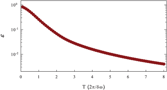
For a rotation and with a typical cut-off value () the amplitude yields a pretty high fidelity of rotation. More precisely, Fig. 2 shows the error for a NOT-gate operation on an arbitrary superposition , which would result in the state , using a Gaussian pulse with cut-off , amplitude and duration time . The leakage outside the qubit manifold, defined as , is also shown in Fig. 3. It is worthwhile noting that although the leakage, for long enough pulses, can be of the order of , the error in the NOT-gate operation is always higher than (see Ref. 21).

IV Quantum optimal control
As we mentioned in the Introduction, in this work we use quantum optimal control theory in order to obtain microwave current modulations which give rise to a high-fidelity NOT-gate operation for a phase qubit. In this section we briefly review the optimal control algorithm which we have employed to obtain optimized modulations.
In general, quantum optimal control algorithms [12, 13, 14] are designed to lead a quantum system with state from an initial state to a target final state at time by minimizing a cost functional which is a measure of inaccuracy of reaching the desired final state. If denotes the state achieved at time , one can consider two different cost functionals:
- •
By minimizing this cost functional, although the population of the desired state will be maximized, the overall phase of this state is not forced to be preserved.
- •
Minimization of this second cost functional, in addition to maximizing the population of the desired state, preserves its overall phase.
In optimal control theory the minimization of the cost functional is done by updating the Hamiltonian of the system, via some control parameters, in an iterative procedure until the desired value of the cost functional is reached. Any specific algorithm which is guaranteed to give improvement at each iteration [22] is called immediate feedback control and can be briefly described as follows: Assume that the Hamiltonian of the system depends on a set of parameters which are controllable. By using a proper initial guess for control parameters, first the state of the system is evolved in time with the initial condition giving rise to after time . At this point the iterative algorithm starts, aiming at decreasing the cost functional by adding a correction to control parameters in each step. In the th step of this iterative algorithm
- •
An auxiliary state is evolved backward in time starting from reaching .
In the case of minimizing , and for minimizing , .
- •
The states and are evolved forward in time, respectively, with control parameters and . Here,
(6) are updated control parameters. is a weight function used to fix initial and final conditions on the control parameters in order to avoid major changes at the beginning and end of time evolution and is an important parameter for the convergence of the algorithm.
These two steps are repeated until the desired value of or is obtained.
In order to implement the optimization procedure to a NOT-gate for any arbitrary superposition of computational states, one must be able to flip and at the same time (i. e. with same pulse) making sure that the phase relation between them is preserved. This is guaranteed by using the following definition of fidelity
| (7) |
where and are final states achieved at time after applying the same pulse on initial states and . The minimization of the cost functional , for flipping at the same time the states and , does not necessarily lead to maximization of the fidelity (7) due to possible changes in the phase relation between them. However if is minimized, the maximal fidelity is also guaranteed. Therefore in order to obtain a high-fidelity NOT-gate it seems more natural to minimize instead of . However, in the following we will show that, although in the ideal case optimized pulses obtained from minimizing result in much higher fidelity, when more realistic cases are considered optimized pulses from minimizing lead to higher fidelities, specially for very short pulses. In this work we often use the error instead of fidelity.
V Numerical Results
In this section we present the numerical results to show that the quantum optimal control theory allows to optimize the modulation of microwave pulses in order to implement a high-fidelity NOT-gate. The optimization is done in the rotating frame and the Hamiltonian (4) is used for time evolution while are calculated by means of perturbation theory.
V.1 Optimal NOT-gate
 |
By employing the quantum optimal control algorithm described in the Sec. IV and using the modulation of the microwave pulse as the control parameter, we start from Gaussian pulses (5) of given duration time as the initial guess and optimize the NOT-gate operation. We will show the results obtained from minimizing both and and refer to corresponding errors by and and corresponding optimized pulses by and . The optimization has been stopped when either the cost functionals reached the value or 5000 iterations are done.
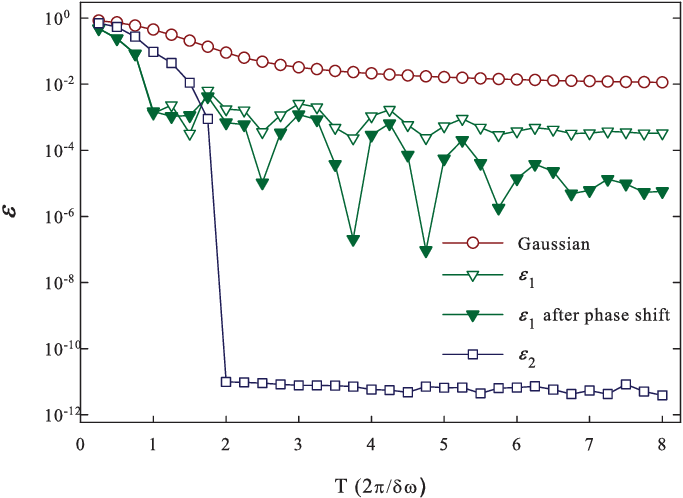
Figure 4 shows the error , as a function of duration time of the pulse , for the Gaussian pulses used as initial guess (circles) and for the optimized pulses (unfilled triangles and squares). For most of points, the convergence is reached in much less than 5000 iterations. However for pulses with , 5000 iterations has been completed. As we expected, minimizing results in high-fidelity NOT-gate with for all ns, while for very short pulses it seems that, with same number of iterations, minimizing leads to better results.
In order to understand the reason for the oscillating behavior of as a function of , we plot the average value of for and transitions at the end of optimization (top panel of Fig. 5) which shows that the final value of for both of these transitions is of the order of . As we explained in Sec. IV, is insensitive to the phase of the final state and it turns out that while a given optimized pulse applied to initial state leads to the final state , then the same pulse might transform the initial state into , i. e. there is a phase difference between the two final states . The bottom panel of Fig. 5 shows this phase difference for optimized pulses with given duration time which increases the error of NOT-gate to what has been shown in Fig. 4.
Although this phase difference causes a major increase in the error while working with superpositions, the error is at least one order of magnitude smaller than those from Gaussian pulses (Fig. 4). Moreover the final phase difference between and can be compensated by a following phase shift gate. In Fig. 4 results after applying a (which is approximately the average of in time) phase shift are also shown (filled triangles) which demonstrate a significant decrease of .
V.2 Imperfections in the pulse shapes
 |
In this section we study the Fourier transform of the optimized pulses, in order to see how practically they are realizable in the laboratory, and to examine the effect of high-frequency components. Two examples of the final optimized pulses (dashed lines) are shown in Fig. 6, both with duration time ns. Optimized (top panel) and (bottom panel) are the results of minimizing, respectively, and which for both are of the order of . The corresponding Gaussian pulse is also shown in both panels. is guaranteed to decrease the error of NOT-gate two orders of magnitude with respect to the Gaussian pulse while would reduce the error up to ten orders of magnitude.
 |
Fig. 7 shows the Fourier transform of the two optimized pulses shown in Fig. 6. To filter out the high-frequency components of the optimized pulses we set a cutoff frequency for Fourier components and apply the truncated pulses again and obtain the error. Fig. 8 shows the error for a NOT-gate for pulses with different duration times as functions of . is approximately GHz and is typically of . In our calculation which means that MHz.
In the case of , top panel of figure 8 makes clear that all important harmonics have frequencies smaller than . Note that the number of harmonics included within the cutoff is equal to so that, for , such number is equal to N times the ratio . As a result it seems that, for all values of considered, about 20 harmonics should be sufficient to reach the smallest value of . , though, seems to be more sensitive to high-frequency components but still about four orders of magnitude smaller than under the cutoff .

V.3 Effect of off-resonance terms

As we mentioned before, we have assumed that off-resonance elements of the Hamiltonian (3) in the rotating frame are negligible and we have used Hamiltonian (4) for calculating the evolution. In this section we check this assumption by addressing the effect of off-resonance elements by evolving the complete Hamiltonian (3) using the optimized pulses obtained using Hamiltonian (4). Top panel of Fig. 9 shows the error for a NOT-gate operation implemented by Gaussian (circles) and optimized pulses from minimizing (triangles) and (squares). For the optimized pulses yield a much higher error, with respect to the case when off-resonance terms are neglected, still showing an improvement of two orders of magnitude if compared to Gaussian pulses. Bottom panel of Fig. 9 shows the absolute value of the error difference obtained by subtracting the error without off-resonance term from the error with off-resonance terms. These figures make clear that while for Gaussian pulses off-resonance terms can be neglected, for optimized pulses, specially those obtained from minimizing , they are very important. Note that, contrary to the ideal case where was about eight orders of magnitude smaller than , under the effect of off-resonance terms, seems to be larger than specially for very short pulses with . This means that the assumption of ignoring these terms is more accurate when is minimized. The simpler shape of the optimized pulses obtained from minimization of could be a reason for that.
V.4 Effect of capacitive interaction
So far we have considered a single qubit with three energy levels and obtained the modulation of the microwave pulses in order to optimize the NOT-gate operation for the two lowest energy states and . It is now interesting to consider the setup [10] containing two qubits interacting via a capacitor. The question that we want to address is what happens if these optimized pulses are applied on the first qubit while the interaction with the second qubit is present.
The interaction Hamiltonian of a circuit with two identical phase qubits has the following form:
| (8) |
where and are Josephson phases across the junction and and is the capacitance of the interaction capacitor. Note that the term with second derivative in Eq. (8) can be included in the Hamiltonians of the uncoupled qubits (1) by replacing the charging energy with an effective one , where and . The Hamiltonian can again be written in the basis of the eigenstates of the uncoupled qubits, and the strength of the interaction Hamiltonian reduces to . We move to the rotating frame described by the unitary operator
| (9) |
and neglect the off-resonance elements of the resulting Hamiltonian. By applying microwave pulse on the first qubit, our aim is to perform a NOT-gate operation on such qubit (namely, ). Since is typically of few fF and is of the order of pF [9, 10] we find which leads to an interaction strength MHz. Figure 10 shows the error as function of time width of the pulse for both Gaussian (circles) and optimized pulses ( triangles and squares). Although the optimized pulses are obtained for a single qubit system, they still result in smaller error at least for short pulses. These results show the importance of the presence of the capacitive interaction even though the strength of the interaction is small. As it is clear from Fig. 10 for pulses longer than, approximately, ns () the interaction becomes more effective and the error for Gaussian and optimized pulses are very close. Moreover, longer pulses lead to higher value of error contrary to what happens in the case of a single qubit. In this case also for very short pulses () is smaller than and for they are of the same order, although in the ideal case was eight orders of magnitude larger than .

Bottom panel of Fig. 10 shows the absolute value of error difference which is obtained by subtracting the error of ideal case from the error in presence of interaction. is almost the same in all three cases.
VI Leakage
As explained in section II, the two lowest energy levels of a current-biased Josephson junction can be used as and states of a phase qubit. Although it would be desirable to have only two levels inside the potential well of the Fig. 1, this is not the case in experimental setups. So far we have included the leakage by considering only an additional third level and showed that it is possible to optimize the pulses in order to gain high fidelity for a NOT-gate for a single qubit. In typical experiments the number of energy levels inside the well varies between three and five. In order to have a more complete understanding of the leakage, in this section we show some results obtained for a five-level system. Since adding more levels to the system decreases the inhomogeneity of the level-spacing we choose .

Figure 11 shows the error for a NOT-gate implemented by optimized and Gaussian pulses, which are used as initial guess, for different duration times . Similar to the case of three-level system, with same number of iterations, minimization of leads to better results for short pulses while for longer duration times of pulses minimizing results in error of NOT-gate . In the case of minimizing , at least one order of magnitude improvement is achieved for long pulses, although the improvement obtained for pulses with shorter time width are the best. By looking at the average value of for transitions between the states and (top panel of Fig. 12) and the final phase difference between them (bottom panel of Fig. 12), one realizes that, as it was observed in three-level system, considerable amount of is due to the final phase difference . For instance the pulse with results in a phase difference approximately equal to zero and therefore for this pulse is of the order of . A proper phase shift applied after the NOT-gate operation will compensate the phase difference between the final and states and consequently attaining a very high fidelity.
Two examples of pulses with are shown in figure 13. is obtained from minimizing and gives rise to while is supposed to minimize with . It seems that, compared to three-level system, higher frequencies and amplitudes are needed to reach high fidelity of NOT-gate. In three-level system the iterative optimization algorithm is applied at most times to reach such fidelities while with five levels iterations were needed to obtain the results shown in figures 11 and 12. The leakage out of the qubit manifold would be the reason for this.


VII Conclusions
In this paper we have shown that it is possible to optimize single-qubit gates for Josephson phase qubits by employing quantum optimal control theory. We have considered the realistic situation in which, in addition to the two computational basis states and , higher energy states are present, which may lead to leakage. Typically microwave pulses with Gaussian modulation are used to induce transition between states and , yielding a quite high fidelity for long pulse durations. For the sake of definiteness, here we have focused on the NOT-gate single-qubit operation and searched for modulations of microwave pulses which optimize such operation, especially for short-duration pulses. The numerical results obtained for a three-level system, and neglecting off-resonance terms, demonstrate up to ten orders of magnitude improvement in fidelity of a NOT-gate operation with respect to those obtained through Gaussian modulations. To test the effect of possible imperfections in the pulses shape, we have studied the behavior of the fidelity as a function of the bandwidth of the pulse generator and showed that frequencies not bigger GHz are needed to gain up to four orders of magnitude improvement. Moreover, we have shown that the off-resonance elements of the Hamiltonian, which are usually neglected, can be important for optimized pulses, especially for short pulse duration times, due to the very high fidelity reached. We have also addressed the effect of the presence of a capacitively-coupled second qubit and showed that, even though the optimized pulses are obtained for a single qubit, they still lead to a high fidelity for a NOT-gate (up to two orders of magnitude improvement) especially for very short pulses. Finally, we were able to obtain optimized pulses for a system with 5 energy levels in which the leakage outside qubit manifold is more severe.
In conclusion, the two-interacting-qubit system deserves for sure further attention. On the one hand, in order to improve the fidelity of a single-qubit operation, in the presence of capacitive coupling, it seems that a way to switch the interaction on and off should be found even for optimized pulses of an isolate qubit. On the other hand, obtaining optimized pulses while including the interaction, would be a potential theoretical work to be done.
Acknowledgements.
We would like to acknowledge fruitful discussions with F. W. J. Hekking. We acknowledge support by EC-FET/QIPC (EUROSQIP) and by Centro di Ricerca Matematica “Ennio De Giorgi” of Scuola Normale Superiore. S. M. acknowledges support by EU-project SCALA.References
- [1] M. A. Nielsen and I. L. Chuang Quantum Computation and Quantum Information (Cambridge, 2000).
- [2] Y. Makhlin, G. Schön and A. Shnirman, Rev. Mod. Phys. 73, 357 (2001).
- [3] G. Wendin and V. S. Shumeiko, Fiz. Nizk. Temp. 33, 957 (2007) [Low Temp. Phys. 33, 724 (2007)].
- [4] J.Q. You and F. Nori, Phys. Today 58, 42 (2005)
- [5] J. Clarke and F. K. Wilhelm, Nature 453, 1031 (2008)
- [6] J. M. Martinis, S. Nam, J. Aumentado and C. Urbina, Phys. Rev. Lett. 89, 117901 (2002).
- [7] J. M. Martinis, S. Nam, J. Aumentado, K. M. Lang and C. Urbina, Phys. Rev. B67, 094510 (2003).
- [8] J. Claudon, F. Balestro, F. W. J. Hekking, and O. Buisson, Phys. Rev. Lett. 93, 187003 (2004).
- [9] M. Steffen, M. Ansmann, R. McDermott, N. Katz, R. C. Bialczak, E. Lucero, M. Neeley, E. M. Weig, A. N. Cleland, and J. M. Martinis, Phys. Rev. Lett. 97, 050502 (2006).
- [10] M. Steffen, M. Ansmann, R. C. Bialczak, N. Katz, E. Lucero, R. McDermott, M. Neeley, E. M. Weig, A. N. Cleland, J. M. Martinis, Science 313, 1423 (2006).
- [11] M. Steffen, J. M. Martinis, and I. L. Chuang, Phys. Rev. B68, 224518 (2003).
- [12] A. P. Peirce, M.A. Dahleh, and H. Rabitz, Phys. Rev. A37,4950 (1988)
- [13] A. Borzi, G. Stadler, and U. Hohenester, Phys. Rev. A66, 053811 (2002)
- [14] S.E. Sklarz and D.J Tannor, Phys. Rev. A66, 053619 (2002)
- [15] T. Calarco, U. Dorner, P. Julienne, C. Williams, and P. Zoller, Phys. Rev. A70, 012306 (2004).
- [16] A. Spörl, T. Schulte-Herbrüggen, S. J. Glaser, V. Bergholm, M. J. Storcz, J. Ferber, and F. K. Wilhelm, Phys. Rev. A75, 012302 (2007).
- [17] S. Montangero, T. Calarco, and R. Fazio, Phys. Rev. Lett. 99, 170501 (2007).
- [18] Sh. Safaei, S. Montangero, F. Taddei, and R. Fazio, Phys. Rev. B77, 144522 (2008).
- [19] See also P. Rebentrost and F. K. Wilhelm, arXiv:0808.2680v1
- [20] R. W. Simmonds, K. M. Lang, D. A. Hite, S. Nam, D. P. Pappas, and J. M. Martinis, Phys. Rev. Lett. 93, 077003 (2004).
- [21] R. Fazio, G.M. Palma and J. Siewert, Phys. Rev. Lett. 83 5385 (1999).
- [22] I. R. Sola, J. Santamaria, and D.J. Tannor, J. Phys. Chem. 102, 4301 (1998)