跳到论文正文
W Papers独立论文阅读器 arXiv:0811.2136 论文正文 计算阅读时间 · 0%
引用这篇论文根据当前论文元数据生成,正式投稿前建议核对。


License: arXiv.org perpetual non-exclusive license
arXiv:0811.2136v2 [hep-ph] 21 Nov 2008
\setcaptionwidth

0.8

Flavour Changing at Colliders in the Effective Theory Approach

Renato Batista Guedes Júnior
2008

Acknowledgments

I would like to express my gratitude to all those that have accompanied me in the elaboration of this thesis, in particular, my supervisors, Doctor Rui Alberto Serra Ribeiro dos Santos and Professor Augusto Manuel Albuquerque Barroso. Without their guidance, support, interest and friendship, I would never have been able to pursue this thesis. I would also like to thank Professor Pedro Miguel Martins Ferreira for the assistance he provided at all levels of the research project.

I also thank Professor Orlando Oliveira, Rita Coimbra and Miguel Won for the assistance they provided of the research Project. I must acknowledge Professor António Onofre, Professor Arhrib Abdesslam and Professor Pedro Texeira-Dias for receive me in their research groups and give me all the support. A very special thanks to Steven Warren, Ana Catarina and António Paço to help me in theirs free time in linguistic review.

Finally, I would like to send my thanks to my friends Ana Rajado, António Paço, Filipa Lopes, Filipe Veloso, Inês de Castro, Nuno Castro, Raquel Varela and Renato Texeira. These individuals always helped me to keep my life in context. I am grateful to my office colleagues as well as to the Interdisciplinary Complex of the University of Lisbon and the Center for Theoretical and Computational Physics (CFTC) of the University of Lisbon, where this thesis was carried out, for the use of the physical resources available. This thesis is supported by Fundação para a Ciência e Tecnologia under Contract No. SFRH/BD/19781/2004.

Resumo

Palavras-chave: Quark top, correntes neutrais, violação de sabor, modelos para além do modelo padrão, propriedade dos leptões, flavor symmetries

Nesta tese discutiremos a parametrização de efeitos relacionados com nova física em altas energias, isto é, física para além do modelo padrão (MP) das interacções fortes e electrofracas. Tal parametrização será feita com recurso a um Lagrangiano efectivo deduzido com o pressuposto de que estes novos efeitos só se manifestam para escalas de energia da ordem do T​e​VTeV e, por imposição, este Lagrangiano terá as mesmas invariâncias do MP. Expandiremos este Lagrangiano em ordem ao inverso da escala de energia. Desta forma, ele será composto por uma serie de termos infinitos de acordo com a escala de energia. Posto que cada termo terá uma dimensão de massa específica, podemos alternativamente identificar cada termo pela sua dimensão. Cada termo da expansão é, por sua vez, composto por inúmeras componentes ou operadores (operadores efectivos) dos quais nos serviremos para agrupar ou identificar os mesmos termos. Veremos ainda que o primeiro termo tem dimensão quatro e assumiremos como sendo o Lagrangiano do MP. Assim, aceitamos que a física descrita pelo Lagrangiano efectivo seja, em primeira aproximação, a mesma do MP sendo as correcções descritas pelos restantes termos.

Passaremos a uma fase seguinte onde nos propomos usar o método anteriormente descrito para parametrizar os efeitos de correntes neutras com mudança de sabor (flavour changing neutral current – FCNC) na produção de single quark top (ou apenas single top). De uma forma mais precisa, sabemos que o quark top, sendo a partícula elementar mais massiva da natureza até aqui conhecida, decai quase exclusivamente em b​WbW (onde bb é o quark botton e WW o bosão vectorial de mesmo nome) antes de se hadronizar. Dizemos quase exclusivamente porque as excepções, d​WdW e s​W,sW, são extremamente suprimidas pelos elementos fora da diagonal da matriz de Cabibbo-Kobayashi-Maskawa (CKM). Também, de acordo com o MP, decaimentos neutros do quark top, ou seja, decaimentos em q​g,qg, q​γq\gamma e q​ZqZ (onde qq pode ser o quark up (u) ou ocharm (c), gg o gluão, γ\gamma o fotão e ZZ o bosão vectorial de mesmo nome) são impossíveis a nível árvore – para ajustar a nomenclatura, chamaremos decaimento forte, no caso do gluão e electrofraco no caso do fotão ou do bosão Z.Z. Assim, aliando mecanismo de supressão da matriz CKM com a impossibilidade de existência de correntes neutras com mudança de sabor, o MP prevê uma secção eficaz na produção de single top através de FCNC bastante suprimida. E se, ao contrário das previsões do MP, FCNC ocorre na natureza? Qual seria o impacto dessas correntes neutras na produção de single top? Independentemente da resposta positiva ou negativa para a existência de tais correntes – que não conhecemos, naturalmente – é sempre possível parametrizar esta hipótese através do Lagrangiano efectivo atrás discutido. No nosso estudo, expandiremos este Lagrangiano até a dimensão seis. Esta escolha prende-se com o facto de procurarmos a primeira contribuição para FCNC, ou seja, a primeira contribuição após a do MP. Os termos de dimensão cinco, a primeira contribuição a seguir à do MP, violam o número leptônico e bariônico para além de não contribuírem com qualquer operador para este estudo. Assim, imposto a conservação destas duas quantidades, devemos excluir os operadores de dimensão cinco e avançar para os de dimensão seis. Acordada a dimensão máxima do Lagrangiano efectivo, torna-se necessário encontrar os operadores que possam contribuir para decaimento do quark top com FCNC (t→q​g,t\rightarrow qg, t→q​γt\rightarrow q\gamma e t→q​Zt\rightarrow qZ) e então, derivar as regras de Feynman desses operadores. Assim, seremos capazes de parametrizar as contribuições desses processos para o decaimento do quark top. Mostraremos ainda que estes decaimentos não são independentes: devido à imposição de invariância de gauge, os decaimentos com FCNC electrofracos estão relacionados, ou seja, o decaimento do top em quark+fotão tem impacto no decaimento em quark+Z e vice-versa. Seremos também capazes de relacionar as taxas de decaimento com FCNC com as secções eficazes de produção de single top ou mesmo das produções parciais: produção de t+γ,t+\gamma, t+Zt+Z e t+qt+q (neste último caso qq pode ser um quark qualquer, excepto o quark top). Estamos interessados em particular no efeito combinado (forte e electrofraco) da produção com FCNC do quark top. Uma forma de abordar as FCNC é pela parametrização do espaço onde a sua existência seria observada (ou não). Um dos objectivos centrais desta tese é precisamente confrontar a hipótese de FCNC na produção do quark top com os valores ou limites que serão originados no LHC. Enquanto aguardamos estes dados, é possível confrontar valores obtidos através de parâmetros gerados aleatoriamente com as características previstas para o LHC. Podemos ainda, fixada a taxa de decaimento com FCNC do quark top, estudar como este decaimento influencia os processos de produção de single top, ou seja, definir regiões onde esperamos registar as contribuições para a produção do quark top. Nalguns casos, esta contribuição pode ser registada ou “vista” experimentalmente no LHC. Mesmo em casos onde não é possível registar a taxa de decaimento devido à sua pequena dimensão, encontraremos regiões onde o seu efeito na secção eficaz de produção de single top pode ser registado. Finalmente, faremos algumas considerações sobre a contribuição para produção de t​t¯t\bar{t} devida a FCNC e mostraremos que esta contribuição muito dificilmente poderá ser visto no LHC.

Finalmente, focaremos a nossa atenção no sector leptónico. Seguindo os procedimentos descritos e aplicados no estudo de FCNC, abordaremos o problema relacionado com violação de sabor entre os leptões (lepton flavour violation – LFV), ou seja, faremos uso de operadores de dimensão seis para descrever LFV. Ainda é mister reconhecer que a violação de sabor no sector leptónico é absolutamente proibida pelo MP em todas as ordens. Veremos também que os limites experimentais para tais processos são extremamente fortes (comparativamente com os limites para os processos bariónico envolvendo FCNC). Assim como fizemos no estudo de FCNC, estudaremos os decaimentos envolvendo LFV, descritos pelo decaimento de um leptão mais pesado em três mais leves, tanto através de vértices do tipo lh​ll​γl_{h}\,l_{l}\,\gamma e lh​ll​Z,l_{h}\,l_{l}Z, onde lhl_{h} e lll_{l} são os leptões mais pesado e mais leve, respectivamente, como através de operadores de quatro-fermiões, já aqui referidos. Procederemos da mesma forma que no sector bariónico para estabelecer relações entre a taxa de decaimento e as secções eficazes dos processos que envolvem LFV, nomeadamente os processos que podem ocorrer no ILC, a colisão entre electrão e positrão resultando em μ−​e+,\mu^{-}\,e^{+}, τ−​e+\tau^{-}\,e^{+} e τ−​μ+\tau^{-}\,\mu^{+} bem como os processo conjugados de carga. Veremos que de acordo com os parâmetros do ILC, tais processos podem ser visto e, inclusive, o seu estudo é bastante facilitado recorrendo a alguns simples procedimentos para a análise do sinal, tais como cortes simples do momento transverso. Por fim, chamamos a atenção para um aspecto muito importante referente às nossas conclusões: todas as relações e parametrizações referenciadas anteriormente entre taxas de decaimento e secções eficazes não se esgotam com este trabalho, antes pelo contrário. Será necessário proceder à referida parametrização de acordo com os dados experimentais que nos chegarão do LHC num futuro bem próximo, ou ainda do ILC (neste caso num futuro cada vez mais distante), mas que hoje mesmo abundam provindo de outros aceleradores. Portanto, há muitos aspectos a serem estudados e muitas simulações a serem feitas. Dito isto, um fio condutor de toda esta tese será a apresentação de todas as expressões analíticas (decaimentos e secções eficazes anómalas), para que os nossos colegas experimentalistas possam proceder a simulações com os seus geradores de Monde-Carlo e definir as possíveis regiões onde poderemos assinalar nova física ligada a processos com FCNC e LFV.

Abstract

Keywords: Top quarks, neutral currents, flavour violation, models beyond the standard models, leptons properties, flavor symmetries

In this thesis we will discuss the parameterisation of effects related with new physics in high energies, that is, physics beyond the standard model (SM) of the strong and electroweak interactions. Such parameterization will be made with resource to an effective Lagrangian deduced considering that these new effects can only be seen energy scale of the order of TeV and, we force, this Lagrangian to be invariancies under the same symmetries. We will expand this Lagrangian to the inverse of the energy scale. This way, it will be composed of a series of infinite terms in accordance with the energy scale. Since each term will have a specific mass dimension, we can alternatively identify each term by its dimension. Each term of the expansion is, in turn, made of innumerable components or operators (effective operators) which we will use to group or identify the same terms. We will also see that the first term has dimension four and will assume it as being the Lagrangian of the SM. Thus, we accept that the physics described by the effective Lagrangian is in a first approach, the same of the SM, while the corrections are described by the remaining terms.

We will then proceed to the next phase where we propose to use the above mentioned method to parameterize the effects of flavour-changing neutral current (FCNC) in the production of single top quark (or just single top). We know that the top quark, being nature’s most massive elementary particle known so far, decays almost exclusively to b​WbW (where bb is the bottom quark and WW the weak boson) before it hadronizes. We say almost exclusively because the exceptions, d​WdW e s​WsW, are extremely suppressed by the off-diagonal elements of the Cabibbo-Kobayashi-Maskawa matrix (CKM). Also, in accordance with the SM, top quark neutral decays, meaning decays in q​g,qg, q​γq\gamma and q​ZqZ (where qq may be the up (u) or charm (c) quark, gg the gluon, γ\gamma the photon e ZZ the vector boson) are impossible at tree level. To adjust the nomenclature, we will name it strong decay in the case of the gluon, and electroweak in the case of the photon or the ZZ boson. Therefore, the CKM matrix suppression mechanism together with the impossibility of FCNC, makes a tiny prediction for values of the cross section in the SM. But what if, contradicting the SM forecasts, FCNC happens in nature more than what the SM forecast? Which would be the impact of these neutral currents in the production of single top? Whether the answer to these questions is positive or negative - which, of course, we do not know – it is always possible to parameterize this hypothesis through the above mentioned effective Lagrangian. In our study we will expand this Lagrangian to dimension six. This choice is due to the fact that we are looking for a first contribution for the FCNC, that is, the first contribution after the SM. The terms of dimension five, which would be the first contribution after the SM, violate the leptonic and barionic number. In addition they do not contribute with any operator to this study. Thus, imposing the conservation of these quantum number, we must exclude dimension five operators and proceed to dimension six operators. Having established the maximum dimension of the effective Lagrangian, it is necessary to find those operators that might contribute to the top quark decay with FCNC (t→q​g,t\rightarrow q\,g, t→q​γt\rightarrow q\,\gamma e t→q​Zt\rightarrow q\,Z) and then, to derive the corresponding Feynman rules. Thus, we will be able to parameterize the contributions of these processes to the top quark decay. We will also show that these decays are not independent - due to the imposition of gauge invariance, electroweak FCNC are related, that is, top quark decay in quark+photon has an impact in quark+ZZ quark decay and vice versa. We will also be able to relate FCNC decay with the cross sections of production of single top or even the partial productions: production of t+γ,t\,+\,\gamma, t+Zt\,+\,Z e t+qt\,+\,q (in this last case q quark can be any quark exception made to the top quark). We are particularly interested in the combined effect (strong and electroweak) of top quark production with FCNC. One way to approach FCNC is through parametrization of the space where its existence would be observed (or not). One of the central aims of this thesis is to confront the hypothesis of FCNC in the production of top quark with the values or limits that will be originated in the LHC. While we wait for these data, it is possible to collate values gotten through parameters randomly generated with the characteristics foreseen for the LHC. Having established the top quark FCNC branching ratio, we still can study how this decay influences the processes of production of single top, that is, to define regions where we hope to register the contributions for the production of top quark. In some cases, this contribution can experimentally be registered or "seen" in the LHC. Even in cases where one cannot register the decay due to its smallest, we will still find regions where its effect in the cross section of single top production can be seen. Finally, we will make some considerations on the contribution of t​t¯t\bar{t} production with FCNC and we will show that this contribution could hardly be seen in the LHC.

Finally, we will focus our attention in the leptonic sector. Following the procedures that we described and applied in the FCNC study, we will approach the problem related with lepton flavour violation (LFV), that is, we will use dimension six operators to describe LFV. We assume that flavour violation in the lepton sector is absolutely forbidden by the SM of all orders. We will also see that the experimental limits for such processes are extremely strong (as compared with the limits for baryonic processes involving FCNC). As in the FCNC study, we will study decays involving LFV, described by a heavier lepton decaing into three lighter leptons, through vertices of the type lh​ll​γl_{h}\,l_{l}\,\gamma e lh​ll​Z,l_{h}\,l_{l}Z, where lhl_{h} e lll_{l} are the heavier and lighter leptons and through four-fermion operators, as described. We will proceed in the same way as in the barionic sector to establish relations between the branching ratios and the cross sections of processes involving LFV, namely the processes that can occur in the ILC or electron-positron collision resulting in μ−​e+,\mu^{-}\,e^{+}, τ−​e+\tau^{-}\,e^{+} and τ−​μ+,\tau^{-}\,\mu^{+}, as well as, the charge conjugate processes. We will see that according to the ILC parameters, such processes can be seen and its study is quite facilitated when we appeal to some simple procedures for the analysis of the signal, such as simple cuts of the transverse moment. Finally, we note that this work does not put an end to all before mentioned relations and parameterizations between branching ratio and cross section. Quite the opposite: it will be necessary to parameterize the experimental data coming from the LHC in the near future, and from the ILC (in a more distant future). Therefore, there are many aspects to be studied and many simulations to be done. This thesis will follow the line of presenting all the analytical expressions (decays and anomalous cross sections), so that our experimentalist colleagues can proceed with the simulation in their Monte-Carlo generators and define the possible regions where we will be able to find new physics in processes with FCNC and LFV.

Preface

The research included in this thesis has been carried out at the Interdisciplinary Complex of the University of Lisbon and the Center for Theoretical and Computational Physics (CFTC) of the University of Lisbon in the Physics Department of the Faculty of Sciences of the University of Lisbon. The list of works published and under review included in this thesis in given below:

  1. 1.

    P. M. Ferreira, R. B. Guedes, and R. Santos, Lepton flavour violating processes at the international linear collider, Phys. Rev. D75, 055015 (2007), hep-ph/0611222 [1];

  2. 2.

    P. M. Ferreira, R. B. Guedes, and R. Santos, Combined effects of strong and electroweak FCNC effective operators in top quark physics at the LHC, Phys. Rev. D77, 114008 (2008), hep-ph/0611222 [2];

  3. 3.

    R. A. Coimbra,P. M. Ferreira, R. B. Guedes, O. Oliveira, R. Santos and Miguel Won, (preparation) [3].

Chapter 1 Introduction

The Large Hadron Collider LHC will soon begin operating. The number of top quarks that will produce is of the order of millions per year. Such large statistics will enable precision studies of top quark physics – this being the least well-know elementary particle discovered so far. The study of flavour changing neutral current (FCNC) interactions of the top quark is of particular interest. In fact, the FCNC decays of the top – decays to a quark of a different flavour and a gauge boson, or a Higgs scalar – have branching ratios which can vary immensely from model to model – from the extremely small values expected within the standard model (SM) to values measurable at the LHC in certain SM extensions.

The use of anomalous couplings to study possible new top physics at the LHC and at the Tevatron has been the subject of many works [4, 15]. The cross section for those processes were calculated in a recent series of papers [16, 17, 18] where FCNC interactions associated with the strong interaction were considered – decays of the type t→u​gt\rightarrow u\,g or t→c​gt\rightarrow c\,g – describing them using the most general dimension six FCNC Lagrangian emerging from the effective operator formalism [19]. The FCNC vertices originating from that Lagrangian also give substantial contributions to production processes of the top quark, such as the associated production of a single top quark alongside a jet, a Higgs boson or an electroweak gauge boson. As we will see, the study of refs. [16, 17, 18] concluded that, for large values of B​R​(t→q​g)BR(t\rightarrow q\,g), with q=u,cq=u,c, these processes of single top production might be observable at the LHC.

Following the treatment of those articles [16, 17, 18], the next logical step is to use the same treatment for the electroweak sector, by considering FCNC interactions leading to decays of the form t→q​γt\rightarrow q\,\gamma or t→q​Z.t\rightarrow q\,Z. In some extensions of the SM these branching ratios can be as large as, if not larger than, those of the strong FCNC interactions involving gluons. In this thesis we extend the analysis of previous works and consider the most general dimension six FCNC lagrangian in the effective operator formalism which leads to t→q​γt\rightarrow q\,\gamma and t→q​Zt\rightarrow q\,Z decays. We will study the effects of these new electroweak FCNC interactions in the decays of the top quark and its expected production at the LHC. We will study in detail processes such as t+γ,t\,+\,\gamma, t+Zt\,+\,Z and t+jt\,+\,j production, for which both strong and electroweak FCNC interactions contribute. The automatic gauge invariance of the effective operator formalism will allow us to detect correlations among several FCNC observables.

As we said, we expect many exciting discoveries to arise from the LHC experiments. However, the LHC is a hadronic machine, and as such precision measurements will be quite hard to undertake there. Also, the existence of immense backgrounds at the LHC may hinder discoveries of new physical phenomena already possible with the energies that this accelerator will achieve. Thus it has been proposed to build a new electron-positron collider, the International Linear Collider [1]. This would be a collider with energies on the TeV range, with extremely high luminosities. The potential for new physics with such a machine is immense. Here, we will focus on a specific sector: the possibility of processes which violate lepton flavour.

We now know that the solar and atmospheric neutrino problems [20] arise not from shortcomings of solar models but from particle physics. Namely, the recent findings by the SNO collaboration [23] have shown beyond doubt that neutrinos oscillate between families as they propagate over long distances. Leptonic flavour violation (LFV) is therefore an established experimental fact. The simplest explanation for neutrino oscillations is that neutrinos have masses that differ from zero – extremely low masses, but nonzero nonetheless. Oscillations with zero neutrino masses are possible, but only in esoteric models [26]. With nonzero neutrino masses, flavour violation in the charged leptonic sector becomes a reality whereas with massless neutrinos, it is not allowed in the SM. This is a sector of particle physics for which we already have many experimental results [27], which set stringent limits on the extent of flavour violation that may occur. Nevertheless, as we will show, even with all known experimental constraints it is possible that signals of LFV may be observed at the ILC, taking advantage of the large luminosities planned for that machine. There has been much attention devoted to this subject. For instance, in refs. [28] effective operators were used to describe LFV decays of the Z boson. LFV decays of the Z boson were also studied in many extensions of the SM [32]. The authors of refs. [39, 42] performed a detailed study of LFV at future linear colliders, originating from supersymmetric models. Finally, a detailed study of the four-fermion operators in the framework of LFV is performed in [43]. In that work the exact number of independent four-fermion operators is determined. Gauge invariance is then used to constrain LFV processes which are poorly measured, or not measured at all. In this work we carry out a model-independent analysis of all possible LFV interactions which might arise in extensions of the SM.

We will follow refs. [2, 3, 1]; as in the articles [16, 17, 18] our methodology will differ from that of previous work in this area; whenever possible, we will present full analytical expressions that our colleagues at the Tevatron or LHC may use in their Monte Carlo generators, to study the sensitivity of the experiments to this new physics. This thesis is organized as follows: in chapter 2 we review the theory obtained through an effective Lagrangian. We expand this Lagrangian in series of 1/Λ1/\Lambda where Λ\Lambda is the energy scale where we suppose our Lagrangian is valid. This allows us to truncate the Lagrangian and make the computation of each term separately following the order that interests us. In our case, we truncate the Lagrangian in the third term, i.e. Λ4,\Lambda^{4}, or dimension six, according to their mass dimension. We justify the assumption that the first term or zero order term matches the SM Lagrangian and, finally, that the terms of order one or dimension five must be ignored for the study of flavour violation. We review the theoretical predictions for the production of t​t¯t\bar{t} and single top quark associated with the FCNC processes, the experimental limits available from the CDF and D0 collaborations of Fermilab as well as the theoretical predictions for LHC. Then, we summarize the experimental limits of the LFV in the leptons colliders.

In chapter 3 we introduce our FCNC operators, explaining what are the physical criteria behind their choice.We also present the Feynman rules for the new anomalous top quark interactions which will be the base of all the work that follows. We use those Feynman rules to compute and analyze the branching ratios of the top quark FCNC decays, with particular emphasis on the relationship between B​r​(t→q​γCLOSEBr(t\rightarrow q\gamma and B​r​(t→q​Z).Br(t\rightarrow qZ). Then we study the cross section for production, at the LHC, of a single top and a photon or a ZZ boson, with all FCNC interactions, both strong and electroweak, included. We also investigate whether or note it would be possible to conclude, from the data, that any FCNC phenomena observed would have at their roots the strong or the electroweak sectors. Finally, we present a general discussion of the results and draw some conclusions.

In chapter 4 we present the effective operator formalism and list the operators which contribute to lepton-violating processes with gauge bosons interactions and four-fermion contact terms. We use the existing experimental bounds on decays such as μ→e​γ\mu\rightarrow e\gamma to exclude several of the operators which could a priori give a contribution to the processes that we will be considering. We also analyze the role that the equations of motion of the fields play in further simplifying our calculations. Having chosen a set of effective operators, we proceed to calculate their impact on LFV decays of leptons, deducing analytical expressions for those quantities. Likewise, we will present analytical results for the cross sections and asymmetries of several LFV processes which might occur at the ILC. Finally, we analyze these results performing a scan over a wide range of values for the anomalous couplings and consider the possible observability of these effects at the ILC.

Chapter 2 Phenomenological Lagrangian and effective operators

We are interested in parameterizing new physics related to top quark physics due to flavour changing neutral current (FCNC) as well as to lepton flavour violation (LFV) in the charged sector. We will discuss this parametrization through an effective theory, that is, using terms of an effective Lagrangian with vertices with flavour violation whose strength must be determined by experimental data.

The experimental data does not provide us with information that allow us to probe new physics beyond the SM. This situation is ripe to change with the introduction of the Large Hadron Collider (LHC) and the construction of the International Linear Collider (ILC). In the first case, we will be searching for new physics through the possibility of FCNC in top quark production at the T​e​VTeV scale. In the second one, we will be looking for LVF. In this chapter, we review the effective Lagrangian technique. After that we explore the limits of these two new manifestations of physics within the SM framework and review the relevant experimental data.

2.1  Effective Lagrangian

The SM has a great success in explaining the most important phenomena at the fundamental level. Nevertheless, it does not have the trademark of a fundamental theory; it has too many parameters and has no prediction regarding the number of particles. The phenomenological success of the SM in the low energy range (the SM was successfully tested in the WW mass range) provides a fundamental constraint to explore physics in the higher energy range. We can suppose that there is a more general theory of which the SM is its low energy limit. The problem is how to describe such a theory.

In general, when we study a system for which we do not have enough experimental information, or for which the theory does not give us enough information about some observation, we can proceed in two ways: a model dependent way (as in supersymmetry, dynamical symmetry breaking technicolor model, etc.) or a model independent way. By model independent we mean the effective Lagrangian approach. In other words, we can parameterize the unknown effects by introducing new terms in the Lagrangian, whose coefficients must be experimentally determined [44, 45, 46, 47, 48, 49]. We must establish the specific way to parametrize these effects according to the specific problems that we have to solve. In this study of FCNC and LFV we do not know this general theory so we can try to describe it through an effective theory i.e. we can try to write an effective FCNC and LFV Lagrangian of the general theory.

When we handle quantum field theory we automatically limit the role that a higher-energy scale (Plank scale) plays in the description of low-energy process. In this sense, the identification of how the scale enters in the calculation provides us with an important way to analyze systems with different scales [48]. The effective theory supplies a tool for exploiting the simplification that arises from systems presenting a large hierarchy of scale. For example, if one assumes that some physical phenomenon is not observed below a certain energy scale Λ,\Lambda, all Fourier components of fields above a scale Λ\Lambda are not directly observable and the Lagrangian of this theory must be obtained by integration over the variable observable at an energy larger then Λ.\Lambda. In this case, a real field – just to simplify – ϕ\phi can be split in two pieces (ϕ=ϕ0+ϕ1\phi=\phi_{0}+\phi_{1}) according to the energy scale such that [46]:

ϕ0​(k→):|k→|<Λϕ1​(k→):Λ<|k→|<Λ1,\phi_{0}(\vec{k}):|\vec{k}|<\Lambda\>\>\>\>\>\phi_{1}(\vec{k}):\Lambda<|\vec{k}|<\Lambda_{1}, (2.1)

where Λ\Lambda is the energy scale and k→\vec{k} the momentum. Then by definition:

ei​Seff=∫[d​ϕ1]​ei​S​[ϕ0,ϕ1]​where​Seff=∫d​x​ℒeff.e^{iS^{\textrm{eff}}}=\int[d\phi_{1}]e^{iS[\phi_{0},\phi_{1}]}\;\;\;\textrm{where}\;\;\;S^{\textrm{eff}}=\int dx\;{\cal L}^{\textrm{eff}}. (2.2)

SeffS^{\textrm{eff}} and ℒeff{\cal L}^{\textrm{eff}} are the effective action and effective Lagrangian respectively. ℒeff\cal{L}^{\textrm{eff}} can be obtained by the expansion of SeffS^{\textrm{eff}} in powers of 1/Λ.1/\Lambda.

To build the effective Lagrangian, one should choose the degrees of freedom to include and the respective symmetries which restrict the possible terms in the effective Lagrangian. The effective Lagrangian has an infinite number of terms each with constant coefficients to be determined experimentally. The effective current-current interaction introduced by Fermi in order to explain the weak interaction is a well-known example of an effective theory.

We have assumed that there is a general theory that we do not know and, that the SM is its low-energy limit. In other words, we must assume that physics beyond the SM is not observed below a certain energy scale Λ.\Lambda. The effective Lagrangian can be expanded in powers of 1/Λ:1/\Lambda:

ℒeff=ℒSM+1Λ​ℒ(5)+1Λ2​ℒ(6)+⋯,{\cal L}^{\textrm{eff}}={\cal L}^{\textrm{SM}}+\frac{1}{\Lambda}{\cal L}^{\textrm{(5)}}+\frac{1}{\Lambda^{2}}{\cal L}^{\textrm{(6)}}+\cdots, (2.3)

where ℒSM{\cal L}^{\textrm{SM}} is the term of order zero and matches the Lagrangian of SM which is not sensitive to the energy scale and has mass-like dimension four. The term ℒ(5){\cal L}^{\textrm{(5)}} is the order one and the mass dimension five and so on. This expansion is convenient because each term is limited by a power of 1/Λ.1/\Lambda. We truncate the above series according to the degree of accuracy we demand. This approach is appropriate for one last reason: it allows us to focus on the phenomenology common to all new physics models [50]. We truncate this series in order two or mass dimension six, ℒ(6).{\cal L}^{(6)}. Let us write ℒ(i){\cal L}^{(i)} as a linear combination of effective operators of dimension ii

ℒ(i)=∑j𝒪j(i)=∑jαj​Oj(i).{\cal L}^{(i)}=\sum_{j}{\cal O}^{(i)}_{j}=\sum_{j}\alpha_{j}O^{(i)}_{j}. (2.4)

where αj\alpha_{j} are unknown parameters which represent the coupling strengths and the subscript ii – i=5,6⋯i=5,6\cdots – denotes the dimension of the Lagrangian term. From this procedure an infinite group of effective operators with the same dimension arises. Finally, we don’t know exactly what the scale is but this is not important for the calculation because we can parameterize the new physics and including Λ\Lambda in the unknown coefficients (see eq. 2.4).

Such an approach has been used by several authors, as can be seen in the following references [4, 15].

2.1.1 The standard Lagrangian ℒSM{\cal L}^{\textrm{SM}}

Now the task is to build all effective operators of a certain dimension respecting the imposed symmetries. The first term is the SM Lagrangian. We will now briefly review the SM Lagrangian.

The standard model of strong and electroweak interaction can be described as a Yang-Mills theory, i.e. the Lagrangian ℒSM\cal{L}^{\textrm{SM}} is locally S​U​(3)×S​U​(2)×U⁡(1)SU(3)\times SU(2)\times U(1) invariant [51, 52]. The symmetry uses 12 gauge vector fields, the gauge bosons. One important aspect of the SM that should be accounted for is that the weak bosons have mass. One can not insert this term into the Lagrangian by hand because such a Lagrangian would not be gauge invariant. A possible mechanism for giving mass to the gauge field was found by Higgs who introduced a complex scalar doublet field ϕ\phi with a non-vanishing vacuum expectation value (vev) – we will use v=<ϕ>=246/2​G​e​Vv=<\phi>=246/\sqrt{2}\,GeV – in the Lagrangian. After spontaneous breaking of the local symmetry the weak bosons acquire mass and a new scalar boson appears, the Higgs boson. This is known as the Higgs mechanism [53].

A realistic model of the electroweak interactions was proposed by Glashow, Salam and Weinberg [55]. It uses two non-equivalent representations for the fermions: the left-handed particles are S​U​(2)SU(2) doublets and the right-handed particles are singlets. In this scheme, the Lagrangian must be S​U​(2)×U⁡(1)SU(2)\times U(1)11 1 We remind that the vector fields (BμCLOSE(B_{\mu} and WμiW^{i}_{\mu} with OPENi=1,2,3)i=1,2,3) are not the physical fields. The physical fields AμA_{\mu}, ZμZ_{\mu} and Wμ±W^{\pm}_{\mu} related to the later by the Weinberg angle. invariant. After spontaneous symmetry breaking, the gauge fields of the weak interaction become massive. Like the boson fields, we cannot insert the fermion mass terms by hand as it is not S​U​(2)×U⁡(1)SU(2)\times U(1) invariant as well. The masses of the fermions are generated by a mechanism similar to that of the bosons in the well-known Yukawa Lagrangian 22 2 The strong interaction between the quarks, known as quantum chromodynamics (QCD), appears when one includes S​U​(3)SU(3) invariance [57]..

In order to establish the notation, we will describe the Lagrangian of the SM. First, the fields: the left-handed lepton doublet and right-handed charged lepton are represented by ℓL\ell_{L} and eR,e_{R}, respectively; the left-handed quark doublets by qLq_{L} and right-handed quarks by uRu_{R} and dRd_{R}; finally, the Higgs boson doublet by ϕ.\phi.

The gauge fields are:

gluons:\displaystyle\textrm{gluons}: Gμa,a=1​…​8,\displaystyle\;G_{\mu}^{a},\>\>\>a=1...8,
Gμ​νa=∂μGνa−∂νGμa+gS​fa​b​c​Gμb​Gνc;\displaystyle\;G_{\mu\nu}^{a}=\partial_{\mu}G_{\nu}^{a}-\partial_{\nu}G_{\mu}^{a}+g_{S}f_{abc}G_{\mu}^{b}G_{\nu}^{c};
W​ bosons:\displaystyle W\;\;\textrm{ bosons}: WμI,I=1​…​3,\displaystyle\;W_{\mu}^{I},\>\>\>I=1...3,
Wμ​νI=∂μWνI−∂νWμI+g​ϵI​K​J​WμK​WνJ;\displaystyle\;W_{\mu\nu}^{I}=\partial_{\mu}W_{\nu}^{I}-\partial_{\nu}W_{\mu}^{I}+g\epsilon_{IKJ}W_{\mu}^{K}W_{\nu}^{J};
B​ bosons:\displaystyle B\;\;\textrm{ bosons}: Bμ,\displaystyle\;B_{\mu},
Bμ​ν=∂μBν−∂νBμ.\displaystyle\;B_{\mu\nu}=\partial_{\mu}B_{\nu}-\partial_{\nu}B_{\mu}. (2.5)

where Gμ​νa,G_{\mu\nu}^{a}, Wμ​νIW_{\mu\nu}^{I} and Bμ​νB_{\mu\nu} are the field strengths of the S​U​(3),SU(3), S​U​(2)SU(2) and U⁡(1)U(1) interactions respectively. The Lagrangian is given by

ℒS​M\displaystyle{\cal L}^{SM} =−14​Gμ​νa​Ga​μ​ν−14​Wμ​νI​WI​μ​ν−14​Bμ​ν​Bμ​ν\displaystyle=-\frac{1}{4}G^{a}_{\mu\nu}G^{a\mu\nu}-\frac{1}{4}W^{I}_{\mu\nu}W^{I\mu\nu}-\frac{1}{4}B_{\mu\nu}B^{\mu\nu}
+(Dμ​ϕ)†​(Dμ​ϕ)+m2​ϕ†​ϕ−12​λ​(ϕ†​ϕ)2\displaystyle+(D_{\mu}\phi)^{\dagger}(D^{\mu}\phi)+m^{2}\phi^{\dagger}\phi-\frac{1}{2}\lambda(\phi^{\dagger}\phi)^{2}
+i​ℓ¯L​D̸​ℓL+i​e¯R​D̸​eR+i​q¯L​D̸​qL+i​u¯R​D̸​uR+i​d¯R​D̸​dR\displaystyle+i\bar{\ell}_{L}\not{D}\ell_{L}+i\bar{e}_{R}\not{D}e_{R}+i\bar{q}_{L}\not{D}q_{L}+i\bar{u}_{R}\not{D}u_{R}+i\bar{d}_{R}\not{D}d_{R}
+Γe​ℓ¯L​eR​ϕ+Γu​q¯L​uR​ϕ~+Γd​q¯L​dR​ϕ+h.c.,\displaystyle+\Gamma_{e}\bar{\ell}_{L}e_{R}\phi+\Gamma_{u}\bar{q}_{L}u_{R}\tilde{\phi}+\Gamma_{d}\bar{q}_{L}d_{R}\phi+h.c., (2.6)

where

Dμ=∂μ−igsλa2Gaμ−igτI2WIμ−ig′YBμD_{\mu}=\partial_{\mu}-ig_{s}\frac{\lambda^{a}}{2}G^{a}_{\mu}-ig\frac{\tau^{I}}{2}W^{I}_{\mu}-ig^{\prime}YB_{\mu} (2.7)

is the covariant derivative and Γℓ,qu,qd\Gamma_{\ell,q_{u},q_{d}} are Yukawa couplings for the leptons, up quarks and down quarks, respectively. λa\lambda^{a} acts on colour or S​U​(3)SU(3) indices, τI\tau^{I} on S​U​(2)SU(2) indices and YY is the hypercharge with value assigned as follows: Y⁡(ℓL)=−12,Y(\ell_{L})=-\frac{1}{2}, Y⁡(er)=−1,Y(e_{r})=-1, Y⁡(qL)=16,Y(q_{L})=\frac{1}{6}, Y⁡(uR)=23,Y(u_{R})=\frac{2}{3}, Y⁡(dR)=−13Y(d_{R})=-\frac{1}{3} and Y⁡(ϕ)=12.Y(\phi)=\frac{1}{2}.

A final feature of the SM is that it is a renormalizable theory [58]: a Yang-Mills theory with spontaneous symmetry breaking is a renormalizable theory if the mass dimension of the Lagrangian is less than or equal to four, in four space-time dimensions.

2.1.2 Dimension five and six effective operators

While the choice of the symmetry limits the number of possible terms in the Lagrangian for each order it is obvious that this does not determine which terms are responsible for a particular manifestation of new physic. For example, the term ℒ(6){\cal L}^{\textrm{(6)}} has 80 effective operators (plus hermitic conjugate) i.e. there are 80 different ways to link together the “SM fields” in an S​U​(3)×S​U​(2)×U⁡(1)SU(3)\times SU(2)\times U(1) invariant operator with mass dimension six and subject to the same broken symmetry as the SM. Some of these operators have only vector bosons. It is obvious that these operators are not important if we are studying LFV because it is not possible to obtain any vertices with flavour violation. Thus, the choice of operators to include in the Lagrangian depends on the problem we are studying.

We will see that the term ℒ(5){\cal L}^{\textrm{(5)}} has no interest to us. However, its simplicity may help us illustratring the general construction of the operators.

The ℒ(5){\cal L}^{\textrm{(5)}} operators are, in principle, all possible combinations of the fields and derivatives building a scalar singlet with mass dimension five. It is not possible to create such an operator, for example, with a fermionic field because such an operator would have at least dimension six. Also, it is not possible to make a dimension five operator with scalar only because we would need five of such fields and it is not possible to put together five doublets in a singlet. In the same way we can eliminate all operators made up by vectors only, fermions and vectors, scalar and vectors and, finally, vectors, fermion and scalar together.

One possible candidate would be to have two fermions and two scalars. If we choose ϕ\phi e ϕ∗\phi^{*} as scalar, the hypercharge must be zero. This is only possible if we use the fermion and its hermitian conjugate. But this is not a gauge invariant scalar. As an alternative, we can use two fields: ϕ\phi and its conjugate field defined as ϕ~=i​σ2​ϕ∗\tilde{\phi}=i\,\sigma_{2}\,\phi^{*} in an S​U​(2)SU(2) triplet. For fermions, we must have two doublets of S​U​(2)SU(2) to form a scalar. This can be achieved using a fermion field Ψ\Psi and its conjugate Ψc.\Psi^{c}. Its components ψc\psi^{c} transform according to 33 3 The relation is the same well known relation between the plane wave solution to the Dirac positive energy solution uu and negative one v:v: v=i​γ2​u∗.v=i\,\gamma_{2}\,u^{*}.

ψc=i​γ2​ψ∗.\psi^{c}=i\,\gamma_{2}\,\psi^{*}. (2.8)

The conjugate doublet Ψc,\Psi^{c}, like Ψ,\Psi, is a helicity state so both transform in the same way under S​U​(2).SU(2). From the chiral or helicity projections γL,R\gamma_{L,R} definition:

γR,L=1±γ52;\gamma_{R,L}=\frac{1\pm\gamma_{5}}{2}; (2.9)

and its commutation relation with Dirac matrix, we have

(ΨL)c\displaystyle(\Psi_{L})^{c} =(Ψ)Rc,\displaystyle=(\Psi)^{c}_{R},
(ΨR)c\displaystyle(\Psi_{R})^{c} =(Ψ)Lc.\displaystyle=(\Psi)^{c}_{L}. (2.10)

Following this, only one operator is left for the leptons and quarks. That is

ℒ(1)\displaystyle{\cal L}^{(1)} =ℓ¯Rc​ϕ​ϕ~​ℓL+h.c.,\displaystyle=\bar{\ell}^{c}_{R}\,\phi\,\tilde{\phi}\,\ell_{L}\,+\,h.c., (2.11)

where ℓc\ell^{c} is the lepton conjugate doublet and is similar to the baryon one. We note that this operator is written as a Majorana mass term ℓ¯Rc​ℓL.\bar{\ell}^{c}_{R}\,\ell_{L}\,.

Finally, ℒ(5){\cal L}^{(5)} breaks baryon and lepton quantum number so we do not need to worry about it as we demand the conservation of these quantum nunbers. Even in the neutral sector, through seesaw mechanism, the neutrino mass (Dirac mass) mν∼10−2​G​e​Vm_{\nu}\sim 10^{-2}\;GeV requires a Majorana mass mR∼1016​G​e​Vm_{R}\sim 10^{16}\;GeV for a scale of 1​G​e​V1\;GeV [59]. This is a typical scale of grand unified theories but it is clearly out of the reach of the next colliders. We are interested in flavour-violation with lepton and baryon number conservation.

The next term is the dimension six ℒ(6).{\cal L}^{(6)}. It is possible to build 80 (plus hermitian conjugate) of such effective operators and the corresponding list can be obtained in [19]. Now we describe any possible kind of operator according to the fields they contain and we exemplify each class with an effective operator:

Vectors Only:

there are four such operators and all are make up of three GG or three WW vector bosons. For example, OG=fa​b​c​Gμa​ν​Gνb​λ​Gλc​μ.O_{G}=f_{abc}G_{\mu}^{a\nu}G_{\nu}^{b\lambda}G_{\lambda}^{c\mu}. The vector arise in the operator either though their field strengths or covariant derivative;

Fermions Only:

these are four-fermion operators and all of them satisfy fermion number conservation. There are four different groups of operators and they are of the form L¯​L​L¯​L,\bar{L}L\bar{L}L, R¯​R​R¯​R,\bar{R}R\bar{R}R, L¯​R​R¯​L\bar{L}R\bar{R}L and L¯​R​L¯​R,\bar{L}R\bar{L}R, where LL and RR are left-handed and right-handed fields, respectively. Below, is an example for each group (we use lepton and baryon fields indiscriminately):

L¯​L​L¯​L:\bar{L}L\bar{L}L:

Oℓ​ℓ(1)=12​(ℓ¯L​γμ​ℓL)​(ℓ¯L​γμ​ℓL).O^{(1)}_{\ell\ell}=\frac{1}{2}(\bar{\ell}_{L}\gamma_{\mu}\ell_{L})(\bar{\ell}_{L}\gamma^{\mu}\ell_{L}).

R¯​R​R¯​R:\bar{R}R\bar{R}R:

Oe​e=12​(e¯R​γμ​eR)​(e¯R​γμ​eR).O_{ee}=\frac{1}{2}(\bar{e}_{R}\gamma_{\mu}e_{R})(\bar{e}_{R}\gamma^{\mu}e_{R}).

L¯​R​R¯​L:\bar{L}R\bar{R}L:

Oℓ​e=(ℓ¯L​eR)​(e¯R​ℓL).O_{\ell e}=(\bar{\ell}_{L}e_{R})(\bar{e}_{R}\ell_{L}).

L¯​R​L¯​R:\bar{L}R\bar{L}R:

Oq​q(1)=(q¯L​uR)​(q¯L​dR).O^{(1)}_{qq}=(\bar{q}_{L}u_{R})(\bar{q}_{L}d_{R}).

For our study, this family of operators has special interest because they are responsible for the four-fermion operator with flavour change;

Scalars Only:

these operators have either six bosons or four bosons and two derivatives. An example of both is: Oϕ=13​(ϕ†​ϕ)3O_{\phi}=\frac{1}{3}(\phi^{\dagger}\phi)^{3} and O∂ϕ=12​∂μ(ϕ†​ϕ)​∂μ(ϕ†​ϕ);O_{\partial\phi}=\frac{1}{2}\partial_{\mu}(\phi^{\dagger}\phi)\partial^{\mu}(\phi^{\dagger}\phi);

Fermions and vectors:

these operators require two fermions and three other powers of mass that can come via a covariant derivative and one field strength. Here is an exemple: Oℓ​W=i​ℓ¯L​τI​γμ​Dν​ℓl​WI​μ​ν;O_{\ell W}=i\bar{\ell}_{L}\tau^{I}\gamma_{\mu}D_{\nu}\ell_{l}W^{I\mu\nu};

Scalars and vectors:

the ϕ\phi and ϕ†\phi^{\dagger} must come in equal numbers in order to ensure S​U​(2)×U⁡(1)SU(2)\times U(1) invariance. With just one of each scalar field we can use two fields strengths, one fields strengths and two covariant derivatives or four covariant derivatives44 4 In the last case we can use the equation of motion and split this operators in fermion fields only. The equation of motion to ϕ†\phi^{\dagger} is D2​ϕ−Γe†​e¯​ℓ+i​Γu​q¯​σ2​u−Γd†​d¯​q.D^{2}\phi-\Gamma^{\dagger}_{e}\bar{e}\ell+i\Gamma_{u}\bar{q}\sigma_{2}u-\Gamma^{\dagger}_{d}\bar{d}q.. In the case of two of each scalar field one can have two covariant derivatives with act ont two diferents fields – (Dμ​ϕ†)​ϕ+ϕ†​Dμ​ϕ.(D^{\mu}\phi^{\dagger})\phi+\phi^{\dagger}D^{\mu}\phi. Applying the equation of motion one obtain operators like Oϕ​G=12​(ϕ†​ϕ)​Gμ​νa​Ga​μ​ν;O_{\phi G}=\frac{1}{2}(\phi^{\dagger}\phi)G^{a}_{\mu\nu}G^{a\mu\nu};

Fermions and scalars:

in this case one must have two fermions and three bosons or two bosons and one derivative which acts on a gauge invariant quantity. These operators are for example Oe​ϕ=(ϕ†​ϕ)​(ℓL​eR​ϕ);O_{e\phi}=(\phi^{\dagger}\phi)(\ell_{L}e_{R}\phi);

Vectors, fermions and scalars:

one can separate two situations: two fermions and one scalar or two scalar. In the first case, we can have two covariant derivatives or one field strength. The two covariant derivative can act both on scalar field, one on the scalar field and one on a fermion or both on the fermions. An example of this kind of operators is: OD​e=(ℓ¯L​Dμ​eR)​Dμ​ϕ.O_{De}=(\bar{\ell}_{L}D_{\mu}e_{R})D^{\mu}\phi.

In the case with two scalar fields one must have one covariant derivative. From the hypercharge assignments the only possibility is the derivative act in the scalar. An example of these fields: Oϕ​ℓ=i⁡(ϕ†​Dμ​ϕ)​(ℓ¯​γμ​ℓ).O_{\phi\ell}=i(\phi^{\dagger}D_{\mu}\phi)(\bar{\ell}\gamma^{\mu}\ell).

We must identify amongst the 80 operators with dimension six all those which are relevant for our research. After this, it is necessary to check if all are linearly independent, that is if they are not connected by the equation of motion or some other operation. If that is the case, we can perform some simplifications. Once the operators are defined, the next step is to determine the Feynman rules (in Appendix 2.A we review the derivation of a Feynman rule) and calculate the processes of interest. So far we have looked at the method from a general point of view. For our work, as mentioned before, we are interested in those processes with FCNC in t​t¯t\bar{t} and single top quark production as well as LFV in the charged sector. Also, we can conclude that in the construction of our effective operators we have to deal with SM terms according to the equation 2.6 and terms of dimension six FCNC and LFV Lagrangian.

We will point out top quark properties and experimental limits of FCNC and LFV, as well as the theoretical framing of the production and expected experimental limits of top quark in the LHC and experimental limits of LFV in the next ILC according SM. The point of this discussion lies on the fact that one can constrain the space of valid solution for flavour violation and identify the conditions for physics beyond SM in the LHC and the ILC.

2.2  FCNC in the top physics

The LHC is a proton-proton collider being constructed at CERN in a tunnel about 100​m100\;m below the ground and with 27​K​m27\;Km in circumference. It’s center-of-mass energy is 14​T​e​V14\;TeV and the expected luminosity is 1034​c​m−2​s−1.10^{34}\;cm^{-2}s^{-1}. Some of its main goals are the search for the Higgs boson, the search for new phenomena such as supersymmetry, extra dimensions, mini black holes and to perform precision measurement of the SM. Particularly relevant to this thesis are the precision measurements related for the production and decay of the top quark.

According to the SM, top quark can be created in pairs via the strong force or singly (single top quark production) via the electroweak interaction.

2.2.1 Top quark-antiquark pairs production

The top quark was discovered at Fermilab in 1995 [60] in the mass range predicted by SM ∼170.9±1.8​G​e​V\sim 170.9\pm 1.8\,GeV [62]. Its large Yukawa coupling in the symmetry breaking sector (due to its big mass) offers the possibility to look for new physics. The top quark, unlike the other quark, decays almost exclusively in t→b​Wt\rightarrow bW before its hadronization due to its extremely short lifetime of ∼4×10⁻²⁵​s.\sim 4\times 10^{-25}\;s. The ratio between the decay time scale and the hadronization time scale is about one order of magnitude. The next decays are t→s​Wt\rightarrow sW and t→d​W,t\rightarrow dW, both suppressed by the square of the CKM matrix elements. Taking |Vt​s|∼0.04|V_{ts}|\sim 0.04 and |Vt​d|∼0.01,|V_{td}|\sim 0.01, we obtain B​r​(t→s​W)∼1.6×10⁻³Br(t\rightarrow sW)\sim 1.6\times 10^{-3} and B​r​(t→d​W)∼1.6×10⁻⁴Br(t\rightarrow dW)\sim 1.6\times 10^{-4} [63].

At the Tevatron, with a center of mass energy s=1.96​T​e​V,\sqrt{s}=1.96\;TeV, top quarks are produced predominantly in pairs via the strong interaction – 85%85\% by q​q¯q\bar{q} annihilation and 15%15\% by gluon-gluon fusion. The corresponding SM cross section in NLO+NNLL55 5 Next-to-leading order + next-to-next-to-leading logarithmic. is 6.77±0.42​p​b6.77\pm 0.42\;pb for a top quark mass of 175​G​e​V175GeV [64] and the Feynman diagrams to this process in the SM are shown in fig. 2.1.

Refer to caption
Figure 2.1: Feynman diagrams for t​t¯t\bar{t} production: (a) and (b) by gluon fusion and (c) by q​q¯q\bar{q} annihilation.

Most of top quarks produced at the LHC – about 833±100​p​b833\pm 100pb [65, 63] – will be quark-antiquark pairs. Of these, approximately 83%83\% will be produced by gluon-gluon fusion and 17%17\% by q​q¯q\bar{q} annihilation.

2.2.2 Single top production

Studying single-top production at hadron colliders is important for a number of reasons: it provides a direct measurement of the CKM matrix element |Vt​b|2;|V_{tb}|^{2}; it measures the spin polarization of top quarks; lastly, the presence of various new non-SM phenomena may be inferred by observing deviations from the predicted rate of the single-top signal [66]. We are particularly interested in this last reason.

There are three electroweak production mechanisms for single top quarks in the SM: tt-channel (q​d→t​d′)(qd\rightarrow td^{\prime}) and (d​d¯′→t​q¯)(d\bar{d}^{\prime}\rightarrow t\bar{q}) as we see in Fig. 2.2-(a) and (b); ss-channel (q​d¯→t​d¯′)(q\bar{d}\rightarrow t\bar{d}^{\prime}) 2.2-(c); associated t​WtW production (g​d→t​W),(gd\rightarrow tW), 2.2-(d) and (e).

Refer to caption
Figure 2.2: Feynman diagrams for electroweak single top production: (a) and (b) t-channel, (c) s-channel, (d) s-channel associated t​WtW production and (e) t-channel associated t​WtW production.

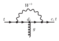
The theoretical single top quark production cross section at the Tevatron is ∼2.9​p​b.\sim 2.9\;pb. Evidence of a single top quark production with a significance of 3.43.4 standard deviation was reported by the D0 Collaboration [67]. The LHC will be able to measure the assumed SM cross section of single top events at NLO to be ∼245±12​p​b\sim 245\pm 12\;pb [68], ∼11±1​p​b\sim 11\pm 1\;pb [69] and ∼66±2​p​b\sim 66\pm 2\;pb [68] for those that occur through the tt -channel, ss -channel and associated t​WtW production, respectively. The neutral coupling preserves flavour; this implies that FCNC are absent at the tree level. In principle, the top production could occur at one loop (see Fig.2.3 for example).
Refer to caption
Figure 2.3: Top quark flavour change to one loop.

Nevertheless, because of Glashow-Iliopous-Maiani (GIM) cancelation [70, 71] the flavour changing related to radiative corrections is suppressed. As such, the branching ratios of these rare top decays are immensely suppressed but can be much larger in extensions of the model. Essentially, in a different theory the existence of new particles will give new contributions to the top rare decays. There can be differences of as much as thirteen orders of magnitude between the SM branching ratios and those in some models, as may be observed in Tab. 2.1.

Process SM QS 2HDM MSSM R​R\!\!\!\!\!\!\not\hskip 9.24994pt SUSY
t→u​Zt\to uZ 8×10−178\times 10^{-17} 1.1×10−41.1\times 10^{-4} −- 2×10−62\times 10^{-6} 3×10−53\times 10^{-5}
t→u​γt\to u\gamma 3.7×10−163.7\times 10^{-16} 7.5×10−97.5\times 10^{-9} −- 2×10−62\times 10^{-6} 1×10−61\times 10^{-6}
t→u​gt\to ug 3.7×10−143.7\times 10^{-14} 1.5×10−71.5\times 10^{-7} −- 8×10−58\times 10^{-5} 2×10−42\times 10^{-4}
t→c​Zt\to cZ 1×10−141\times 10^{-14} 1.1×10−41.1\times 10^{-4} ∼10−7\sim 10^{-7} 2×10−62\times 10^{-6} 3×10−53\times 10^{-5}
t→c​γt\to c\gamma 4.6×10−144.6\times 10^{-14} 7.5×10−97.5\times 10^{-9} ∼10−6\sim 10^{-6} 2×10−62\times 10^{-6} 1×10−61\times 10^{-6}
t→c​gt\to cg 4.6×10−124.6\times 10^{-12} 1.5×10−71.5\times 10^{-7} ∼10−4\sim 10^{-4} 8×10−58\times 10^{-5} 2×10−42\times 10^{-4}
Table 2.1: Branching ratios for FCNC decays of the top quark in the SM and several possible extensions: the quark-singlet model (QS), the two-higgs doublet model (2HDM), the minimal supersymmetric model (MSSM) and SUSY with R-parity violation. See ref. [73, 74, 80] for details.

In the SM these type of decays are so rare that they will never be observed in experiments due to lack of sensitivity (the sensitivity of the experiments at the LHC is of O⁡(10−5)O(10^{-5}) at best [94]).

As we have said, we can parameterize the effects of FCNC through an effective Lagrangian. It is therefore important to use the experimental data to limit the coefficients of operators related with all FCNC. Indirect bounds [95, 96] come from electroweak precision physics and from B and K physics. The strongest bounds so far are the ones in [95] where invariance under S​U​(2)LSU(2)_{L} is required for the set of operators chosen. Top and bottom physics are related and B physics can be used to set limits on operators that involve top and bottom quarks through gauge invariance. Regarding B​r​(t→q​Z)Br(t\,\rightarrow\,q\,Z) and B​r​(t→q​γ)Br(t\,\rightarrow\,q\,\gamma), the only direct bounds available to date are the ones from the Tevatron (CDF). The CDF collaboration has searched its data for signatures of t→q​γt\,\rightarrow\,q\,\gamma and t→q​Zt\,\rightarrow\,q\,Z (where q=u,cq\,=\,u,c). Both analyses use p​p¯→t​t¯p\bar{p}\,\rightarrow\,t\,\bar{t} data and assume that one of the top decays according to the SM into W​bW\,b. The results are presented in Table 2.2.

LEP HERA Tevatron
B​r​(t→q​Z)Br(t\rightarrow q\,Z) < 7.8%<\,7.8\%\,[100] < 49%<\,49\%\, [104] < 10.6%d<\,10.6\%\,^{d} [105]66 6 [VER SE A REFERÊNCIA [105] ACESCENTA ALGO DE NOVO]
B​r​(t→q​γ)Br(t\rightarrow q\,\gamma) < 2.4%<\,2.4\%\, [100] < 0.75%<\,0.75\%\, [104] < 3.2%d<\,3.2\%\,^{d} [106]
B​r​(t→q​g)Br(t\rightarrow q\,g) < 17%<\,17\%\, [63] < 13%<\,13\%\,[107, 104] <O⁡(0.1−1%)<\,O(0.1-1\%)\, [109, 50]
Table 2.2: Current experimental bounds on FCNC branching ratios. The upperscript “d” refers to bounds obtained from direct measurements, as is explained in the text.

The bounds on the branching ratios from LEP and ZEUS are bounds on the cross section that were then translated into bounds on the branching ratios through the anomalous couplings. The LEP bounds use the same anomalous coupling for the uu and cc quarks and the ZEUS bound is only for the process involving a uu quark. The bounds on B​r​(t→q​g)Br(t\rightarrow\,q\,g) are all from cross sections translated into branching ratios. Usually only one operator is considered, the chromomagnetic one, which makes the translation straightforward. The same searches are being prepared for the LHC. A detailed discussion with all present bounds on FCNC and the predictions for the LHC can be found in [110, 94, 111]. With a luminosity of 100​f​b−1100\;fb^{-1} and in the absence of signal, the 95% confidence level expected bounds on the branching ratios are B​r​(t→q​Z)∼ 10−5Br(t\,\rightarrow\,q\,Z)\,\sim\,10^{-5}, B​r​(t→q​γ)∼ 10−5Br(t\,\rightarrow\,q\,\gamma)\,\sim\,10^{-5} and B​r​(t→q​g)∼ 10−4Br(t\,\rightarrow\,q\,g)\,\sim\,10^{-4}. In this thesis, we assume a 10−210^{-2} upper bond of those FCNC branching ratios in except when otherwise mentioned.

2.3  Linear Collider and LFV

Process Upper bound
τ→e​e​e\tau\,\rightarrow\,e\,e\,e 2.0×10−72.0\times 10^{-7}
τ→e​μ​μ\tau\,\rightarrow\,e\,\mu\,\mu 2.0×10−72.0\times 10^{-7}
τ→μ​e​e\tau\,\rightarrow\,\mu\,e\,e 1.1×10−71.1\times 10^{-7}
τ→μ​μ​μ\tau\,\rightarrow\,\mu\,\mu\,\mu 1.9×10−71.9\times 10^{-7}
μ→e​e​e\mu\,\rightarrow\,e\,e\,e 1.0×10−121.0\times 10^{-12}
Z→e​μZ\,\rightarrow\,e\,\mu 1.7×10−61.7\times 10^{-6}
Z→e​τZ\,\rightarrow\,e\,\tau 9.8×10−69.8\times 10^{-6}
Z→τ​μZ\,\rightarrow\,\tau\,\mu 1.2×10−51.2\times 10^{-5}
Table 2.3: Experimental constraints on flavour-violating decay branching ratios [27].

In chapter 4 we will parameterize the possibility of LFV in the charged sector through effective operators. Whereas with massless neutrinos LFV is not allowed in the SM, in the analysis of the signal and background this is a major simplification when compared to the analysis of FCNC. On the other hand, this is a sector of particle physics for which we already have many experimental results [27], all of which set stringent limits on the extent of flavour violation that may occur. Nevertheless, as we will show in this thesis, even with all known experimental constraints, signals of LFV may be observed. The LHC is a hadronic machine, and as such precision measurements will be quite hard to undertake there. Also, the existence of immense backgrounds at the LHC may hinder discoveries of new physical phenomena already possible at the energies that this accelerator will achieve. Thus it has been proposed to build a new electron-positron collider, the International Linear Collider (ILC) [112]. This would be a collider with a center-of-mass energy of ground 1​T​e​V1\;TeV and a planned integrated luminosity of 1​a​b−1.1\;ab^{-1}. The potential for new physics with such a machine is immense.

Finally, in Table 2.3 we present the experimental limits from the branching ratios of lepton decay with flavour-violation. In the final part of the chapter 4 we will discuss the possible improvement of these limits in the existing colliders.

Appendix 2.A Effective operators and Feynman rules

We will give an example of the derivation of the Feynman rules on a dimension six operator [113]

𝒪q​G\displaystyle{\cal O}_{qG} =∑i,jiΛ2​αi​j​q¯i​γμ​λa​Dν​qj​Gμ​νa,\displaystyle=\sum_{i,j}\frac{i}{\Lambda^{2}}\alpha_{ij}\bar{q}^{i}\gamma^{\mu}\lambda^{a}D^{\nu}q^{j}G^{a}_{\mu\nu}, (2.12)

where i,j=1,2,3i,j=1,2,3 correspond to three quark families. As we are interested in flavour violation, we must get i≠ji\neq j and

𝒪q​G\displaystyle{\cal O}_{qG} =∑i≠jiΛ2​αi​j​q¯i​γμ​λa​Dν​qj​Gμ​νa.\displaystyle=\sum_{i\neq j}\frac{i}{\Lambda^{2}}\alpha_{ij}\bar{q}^{i}\gamma^{\mu}\lambda^{a}D^{\nu}q^{j}G^{a}_{\mu\nu}. (2.13)

Taking a particular ii and jj

𝒪~q​G\displaystyle\tilde{\cal O}_{qG} =iΛ2​αi​j​q¯i​γμ​λa​Dν​qj​Gμ​νa+iΛ2​αj​i​q¯j​γμ​λa​Dν​qi​Gμ​νa.\displaystyle=\frac{i}{\Lambda^{2}}\ \alpha_{ij}\bar{q}^{i}\gamma^{\mu}\lambda^{a}D^{\nu}q^{j}G^{a}_{\mu\nu}+\frac{i}{\Lambda^{2}}\alpha_{ji}\bar{q}^{j}\gamma^{\mu}\lambda^{a}D^{\nu}q^{i}G^{a}_{\mu\nu}. (2.14)

The hermitian conjugate of the second term in the right side is:

𝒪~q​G†\displaystyle\tilde{\cal O}^{\dagger}_{qG} =−iΛ2​αj​i∗​q¯i​γμ​D←ν​λa​qj​Gμ​νa.\displaystyle=\frac{-i}{\Lambda^{2}}\alpha^{*}_{ji}\bar{q}^{i}\gamma^{\mu}\overleftarrow{D}^{\nu}\lambda^{a}q^{j}G^{a}_{\mu\nu}. (2.15)

Now, let’s add this term to the first one in the right side of eq. 2.12 and we will designate result by 𝒪q​G{\cal O}_{qG} again

𝒪q​G\displaystyle{\cal O}_{qG} =iΛ2​q¯i​γμ​λa​(αi​j​D→ν−αj​i∗​D←ν)​qj​Gμ​νa.\displaystyle=\frac{i}{\Lambda^{2}}\bar{q}^{i}\gamma^{\mu}\lambda^{a}(\alpha_{ij}\overrightarrow{D}^{\nu}-\alpha^{*}_{ji}\overleftarrow{D}^{\nu})q^{j}G^{a}_{\mu\nu}. (2.16)

According with eg. 2.7, the covariant derivative has a partial derivative whose term generates a triple vertex and the other one is comprised by gauge fields and originates a four vertex. Let’s focus in the triple vertices

𝒪q​G\displaystyle{\cal O}_{qG} =iΛ2​αi​j​q¯i​γμ​λa​(αi​j​∂→ν−αj​i∗​∂←ν)​qj​(∂μGνa−∂νGμa).\displaystyle=\frac{i}{\Lambda^{2}}\alpha_{ij}\bar{q}^{i}\gamma^{\mu}\lambda^{a}(\alpha_{ij}\overrightarrow{\partial}^{\nu}-\alpha^{*}_{ji}\overleftarrow{\partial}^{\nu})q^{j}(\partial_{\mu}G^{a}_{\nu}-\partial_{\nu}G^{a}_{\mu}). (2.17)

Introducing the identity 1=γL+γR1=\gamma_{L}+\gamma_{R} and some manipulation, we get

𝒪q​G\displaystyle{\cal O}_{qG} =iΛ2​[u¯Li​γμ​λa​(αi​j​∂→ν−αj​i∗​∂←ν)​uLj+d¯Li​γμ​λa​(∂→ν−∂←ν)​dLj]​(∂μGνa−∂νGμa)\displaystyle=\frac{i}{\Lambda^{2}}\left[\bar{u}^{i}_{L}\gamma^{\mu}\lambda^{a}(\alpha_{ij}\overrightarrow{\partial}^{\nu}-\alpha^{*}_{ji}\overleftarrow{\partial}^{\nu})u^{j}_{L}+\bar{d}^{i}_{L}\gamma^{\mu}\lambda^{a}(\overrightarrow{\partial}^{\nu}-\overleftarrow{\partial}^{\nu})d^{j}_{L}\right](\partial_{\mu}G^{a}_{\nu}-\partial_{\nu}G^{a}_{\mu})
+iΛ2​u¯Ri​γμ​λa​(αi​j​∂→ν−αj​i∗​∂←ν)​uRj​(∂μGνa−∂νGμa).\displaystyle+\frac{i}{\Lambda^{2}}\bar{u}^{i}_{R}\gamma^{\mu}\lambda^{a}(\alpha_{ij}\overrightarrow{\partial}^{\nu}-\alpha^{*}_{ji}\overleftarrow{\partial}^{\nu})u^{j}_{R}(\partial_{\mu}G^{a}_{\nu}-\partial_{\nu}G^{a}_{\mu}). (2.18)

We can concentrate in the right sector (the left one is similar) so, from eq. 2.18

𝒪q​GR\displaystyle{\cal O}^{R}_{qG} =iΛ2​uR¯i​γμ​γR​λa​(αi​j​∂→ν−αj​i∗​∂←ν)​uj​(∂μGνa−∂νGμa).\displaystyle=\frac{i}{\Lambda^{2}}\bar{u_{R}}^{i}\gamma^{\mu}\gamma_{R}\lambda^{a}(\alpha_{ij}\overrightarrow{\partial}^{\nu}-\alpha^{*}_{ji}\overleftarrow{\partial}^{\nu})u^{j}(\partial_{\mu}G^{a}_{\nu}-\partial_{\nu}G^{a}_{\mu}). (2.19)

The functional Γ⁡[ϕ]\Gamma[\phi] generates the n-point vertex function Γn​(p)\Gamma^{n}(p) and is defined by the Legendre transformation[113]

W⁡[J]=Γ⁡[ϕ]+∫d​x​J​(x)​ϕ​(x),W[J]=\Gamma[\phi]+\int dx\,J(x)\,\phi(x), (2.20)

where J⁡(x)J(x) is the source, ϕ\phi is a generic field of the theory and W⁡[J]W[J] is the generating functional which generates only connected Green’s functions. The relation between Γ⁡[ϕ]\Gamma[\phi] and the Lagrangian is given by

Γ⁡[ϕ]\displaystyle\Gamma[\phi] =∫d4​x​ℒi​n​t​[ϕ].\displaystyle=\int d^{4}x\,{\cal L}_{int}[\phi]. (2.21)

Using the eqs. 2.20 and 2.21 the 3-point vertex function in spacial coordinates are given by

Γλ(3)​(x1,x2,x3)\displaystyle\Gamma^{(3)}_{\lambda}(x_{1},x_{2},x_{3}) =δ3​Γδ​Gλb​(x3)​δ​u¯k​(x2)​δ​ul​(x1)\displaystyle=\frac{\delta^{3}\Gamma}{\delta G^{b}_{\lambda}(x_{3})\delta\bar{u}^{k}(x_{2})\delta u^{l}(x_{1})}
=i​λaΛ2​∫d4​x​δi​l​δ4​(x−x2)​γμ​γR​(αi​j​∂→ν−αj​i∗​∂←ν)​δ4​(x−x1)​δj​k\displaystyle=i\frac{\lambda^{a}}{\Lambda^{2}}\int d^{4}x\delta^{il}\delta^{4}(x-x_{2})\gamma^{\mu}\gamma_{R}(\alpha_{ij}\overrightarrow{\partial}^{\nu}-\alpha^{*}_{ji}\overleftarrow{\partial}^{\nu})\delta^{4}(x-x_{1})\delta^{jk}
×(gν​λ∂μ−gμ​λ∂ν)δ4(x−x3)δa​b.\displaystyle\times\left(g_{\nu\lambda}\partial_{\mu}-g_{\mu\lambda}\partial_{\nu}\right)\delta^{4}(x-x_{3})\delta^{ab}. (2.22)

We use the Fourier transform to get the 3-point vertex function in the momentum space (we use a convention where the uu and GG momenta incoming and the u¯\bar{u} momenta is outcoming). So

T​F\displaystyle TF =(2​π)4​δ4​(p−q+k)​Γλ​(p,q,k)\displaystyle=(2\pi)^{4}\delta^{4}(p-q+k)\Gamma_{\lambda}(p,q,k)
=i​λaΛ2​∫d4​x​d4​x1​d4​x2​d4​x3​e−i⁡(p​x1−q​x2+k​x3)​δ4​(x−x2)​γμ​γR​(αi​j​∂→ν−αj​i∗​∂←ν)​δ4​(x−x1)\displaystyle=i\frac{\lambda^{a}}{\Lambda^{2}}\int d^{4}xd^{4}x_{1}d^{4}x_{2}d^{4}x_{3}e^{-i(px_{1}-qx_{2}+kx_{3})}\delta^{4}(x-x_{2})\gamma^{\mu}\gamma_{R}(\alpha_{ij}\overrightarrow{\partial}^{\nu}-\alpha^{*}_{ji}\overleftarrow{\partial}^{\nu})\delta^{4}(x-x_{1})
×(gν​λ∂μ−gμ​λ∂ν)δ4(x−x3)\displaystyle\times\left(g_{\nu\lambda}\partial_{\mu}-g_{\mu\lambda}\partial_{\nu}\right)\delta^{4}(x-x_{3})
=i​λaΛ2​∫d4​x​d4​x2​d4​x3​e−i⁡(p​x−q​x2+k​x3)​γμ​γR​δ4​(x−x2)​(αi​j​i​pν−αj​i∗​∂←ν)\displaystyle=i\frac{\lambda^{a}}{\Lambda^{2}}\int d^{4}xd^{4}x_{2}d^{4}x_{3}e^{-i(px-qx_{2}+kx_{3})}\gamma^{\mu}\gamma_{R}\delta^{4}(x-x_{2})(\alpha_{ij}ip^{\nu}-\alpha^{*}_{ji}\overleftarrow{\partial}^{\nu})
×(gν​λ∂μ−gμ​λ∂ν)δ4(x−x3).\displaystyle\times\left(g_{\nu\lambda}\partial_{\mu}-g_{\mu\lambda}\partial_{\nu}\right)\delta^{4}(x-x_{3}). (2.23)

Recall that

∫d4​x​∂μδ4​(x)\displaystyle\int d^{4}x\partial^{\mu}\;\delta^{4}(x) =∫d4​x​d4​p​∂μei​pν​xν\displaystyle=\int d^{4}x\;d^{4}p\;\partial^{\mu}e^{ip^{\nu}x_{\nu}}
=i​∫d4​x​d4​p​pν​gμ​ν​ei​pν​xν\displaystyle=i\;\int d^{4}x\;d^{4}p\;p^{\nu}\;g_{\mu\nu}\;e^{ip^{\nu}x_{\nu}}
=i​∫d4​p​pμ​∫d4​x​ei​p⋅x\displaystyle=i\;\int d^{4}p\;p_{\mu}\;\int d^{4}x\;e^{ip\cdot x}
=i​∫d4​p​pμ​δ4​(p)\displaystyle=i\;\int d^{4}p\;p_{\mu}\;\delta^{4}(p)
=i​pμ\displaystyle=i\;p_{\mu} (2.24)

and

T​F\displaystyle TF =iλaΛ2∫d4xd4x3e−i⁡((p−q)​x+k​x3)γμγR(i)(αi​jpν+αj​i∗qν)(gν​λ∂μ−gμ​λ∂ν)δ4(x−x3)\displaystyle=i\frac{\lambda^{a}}{\Lambda^{2}}\int d^{4}xd^{4}x_{3}e^{-i\left((p-q)x+kx_{3}\right)}\gamma^{\mu}\gamma_{R}(i)(\alpha_{ij}p^{\nu}+\alpha^{*}_{ji}q^{\nu})\left(g_{\nu\lambda}\partial_{\mu}-g_{\mu\lambda}\partial_{\nu}\right)\delta^{4}(x-x_{3})
=i​λaΛ2​∫d4​x​e−i⁡(p−q+k)​x​γμ​γR​(i)​(αi​j​pν+αj​i∗​qν)​(i)​(gν​λ​(pμ+qμ)−gμ​λ​(pν+qν)).\displaystyle=i\frac{\lambda^{a}}{\Lambda^{2}}\int d^{4}xe^{-i(p-q+k)x}\gamma^{\mu}\gamma_{R}(i)(\alpha_{ij}p^{\nu}+\alpha^{*}_{ji}q^{\nu})(i)\left(g_{\nu\lambda}(p_{\mu}+q_{\mu})-g_{\mu\lambda}(p_{\nu}+q_{\nu})\right).

Momentum conservation in the vertex implies

T​F\displaystyle TF =i​λaΛ2​∫d4​x​e−i⁡(p−q+k)​x​γμ​γR​(αi​j​pν+αj​i∗​qν)​(kμ​gν​λ−kν​gμ​λ)\displaystyle=i\frac{\lambda^{a}}{\Lambda^{2}}\int d^{4}xe^{-i(p-q+k)x}\gamma^{\mu}\gamma_{R}(\alpha_{ij}p^{\nu}+\alpha^{*}_{ji}q^{\nu})\left(k_{\mu}g_{\nu\lambda}-k_{\nu}g_{\mu\lambda}\right)
=i​λaΛ2​γμ​γR​(αi​j​pν+αj​i∗​qν)​(kμ​gν​λ−kν​gμ​λ)​∫d4​x​e−i⁡(p−q+k)​x\displaystyle=i\frac{\lambda^{a}}{\Lambda^{2}}\gamma^{\mu}\gamma_{R}(\alpha_{ij}p^{\nu}+\alpha^{*}_{ji}q^{\nu})\left(k_{\mu}g_{\nu\lambda}-k_{\nu}g_{\mu\lambda}\right)\int d^{4}xe^{-i(p-q+k)x}
=i​λaΛ2​γμ​γR​(αi​j​pν+αj​i∗​qν)​(kμ​gν​λ−kν​gμ​λ)​(2​π)4​δ4​(p−q+k)\displaystyle=i\frac{\lambda^{a}}{\Lambda^{2}}\gamma^{\mu}\gamma_{R}(\alpha_{ij}p^{\nu}+\alpha^{*}_{ji}q^{\nu})\left(k_{\mu}g_{\nu\lambda}-k_{\nu}g_{\mu\lambda}\right)(2\pi)^{4}\delta^{4}(p-q+k) (2.25)

and replacing 2.23 in the left side of 2.25

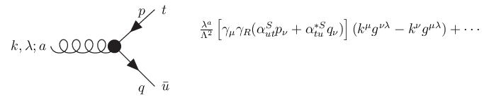
Γλ​(p,q,k)\displaystyle\Gamma_{\lambda}(p,q,k) =i​λaΛ2​γμ​γR​(αi​j​pν+αj​i∗​qν)​(kμ​gν​λ−kν​gμ​λ).\displaystyle=i\frac{\lambda^{a}}{\Lambda^{2}}\gamma^{\mu}\gamma_{R}(\alpha_{ij}p^{\nu}+\alpha^{*}_{ji}q^{\nu})\left(k_{\mu}g_{\nu\lambda}-k_{\nu}g_{\mu\lambda}\right). (2.26)

We represent this vertex by a black circle in the Feynman diagrams. Thus, eq. 2.26 is represented by the fig 2.4
Refer to caption
Figure 2.4: Feynman rules for the g​t​u¯.gt\bar{u}.

where the ellipsis recall that there should be more terms that must be include in this vertex (see fig. 3.3).

Now, we discuss some points that will be useful for this work. According with our convention, the momentum of the boson vector is always entering in the vertex while with the fermions, the momentum is entering in the particle case and leaving in the anti-particle. We have also computed a rule where the boson is represented by a gluon – so this means a strong interaction. The same treatment can be applied to the photon and to the ZZ boson. We will discuss the effective operators responsible for these vertices in the next two chapters.

Chapter 3 Top quark production and decay in the effective Lagrangian approach

According to the previous chapter, the effective Lagrangian can be expanded as

ℒeff=ℒSM+1Λ​ℒ(5)+1Λ2​ℒ(6)+⋯.{\cal L}^{\textrm{eff}}={\cal L}^{\textrm{SM}}+\frac{1}{\Lambda}{\cal L}^{\textrm{(5)}}+\frac{1}{\Lambda^{2}}{\cal L}^{\textrm{(6)}}+\cdots. (3.1)

We truncate this Lagrangian in the order Λ−2\Lambda^{-2} – or dimension six – and ignore the dimension five term. The contributions of order Λ−2\Lambda^{-2} and Λ−4\Lambda^{-4} to the single top quark and t​t¯t\bar{t} production with FCNC are summarized in Tab. 3.1.

1 direct production p​p→(g​q)→tp\;p\rightarrow(g\;q)\rightarrow t\;
2 top + jet production p​p→(g​g)→q¯​t+Xp\;p\rightarrow(g\;g)\rightarrow\bar{q}\;t\;+\;X
p​p→(g​q)→g​t+Xp\;p\rightarrow(g\;q)\rightarrow g\;t\;+\;X
p​p→(q¯​q)→q¯​t+Xp\;p\rightarrow(\bar{q}\;q)\rightarrow\bar{q}\;t\;+\;X
(including 4-fermion interactions)
3 top + anti-top production p​p→(g​g)→t¯​t+Xp\;p\rightarrow(g\;g)\rightarrow\bar{t}\;t\;+\;X
p​p→(q¯​q)→t¯​t+Xp\;p\rightarrow(\bar{q}\;q)\rightarrow\bar{t}\;t\;+\;X
4 top + gauge boson production p​p→(g​q)→γ​t+Xp\;p\rightarrow(g\;q)\rightarrow\gamma\;t\;+\;X
p​p→(g​q)→Z​t+Xp\;p\rightarrow(g\;q)\rightarrow Z\;t\;+\;X
p​p→(g​q)→W​t+Xp\;p\rightarrow(g\;q)\rightarrow W\;t\;+\;X
5 top + Higgs production p​p→(g​p)→H​t+Xp\;p\rightarrow(g\;p)\rightarrow H\;t\;+\;X
Table 3.1: Contributions of order Λ−2\Lambda^{-2} and Λ−4\Lambda^{-4} to the cross section of top production [94].

The FCNC processes p​p→t​Zpp\rightarrow t\,Z and p​p→t​γpp\rightarrow t\,\gamma were studied in great detail for the Tevatron in [114] and for the LHC in [115]. The authors of [16, 17, 18] have presented a complete study of those processes in the strong sector; they have presented a full analytical expression of all processes listed in that table as well as the conditions and limits for their observation at the LHC. The process label in the Tab. 3.1 by 1 and 2 was treated in the article [16, 17] and 3, 4 and 5 in article [18]. Now, our propose is, following refs. [2, 3], to present the same treatment for the electroweak sector i.e. the contribution due the effective FCNC electroweak operators to top quark production; finally we study the combined effects of strong and electroweak effective FCNC operators in top production.

3.1  FCNC effective operators

We are interested in effective operators of dimension six that contribute to flavour-changing interactions of the top quark in the weak sector. As we have said before we do not consider ℒ(5){\cal L}^{(5)} in our analysis. We follow refs. [16, 17, 18], where the authors considered FCNC top effective operators which affect the strong sector. Namely, operators which, amongst other things, contribute to FCNC decays of the form t→u​gt\,\rightarrow\,u\,g or t→c​gt\,\rightarrow\,c\,g. The operators they considered were expressed as

𝒪t​G\displaystyle{\cal O}_{tG} =i​αi​tSΛ2​(u¯Ri​λa​γμ​Dν​tR)​Ga​μ​ν,𝒪t​G​ϕ=βi​tSΛ2​(q¯Li​λa​σμ​ν​tR)​ϕ~​Gμ​νa,\displaystyle=i\frac{\alpha^{S}_{it}}{\Lambda^{2}}\,\left(\bar{u}^{i}_{R}\,\lambda^{a}\,\gamma_{\mu}D_{\nu}t_{R}\right)\,G^{a\mu\nu}\;\;\;,\;\;\;{\cal O}_{tG\phi}=\frac{\beta^{S}_{it}}{\Lambda^{2}}\,\left(\bar{q}^{i}_{L}\,\,\lambda^{a}\,\sigma^{\mu\nu}\,t_{R}\right)\,\tilde{\phi}\,G^{a}_{\mu\nu}\;\;\;, (3.2)

where the coefficients αi​tS\alpha^{S}_{it} and βi​tS\beta^{S}_{it} are complex dimensionless couplings. The fields uRiu^{i}_{R} and qLiq^{i}_{L} represent the right-handed up-type quark and left-handed quark doublet of the first and second generation – this way FCNC occurs. Gμ​νaG^{a}_{\mu\nu} is the gluonic field tensor. There are also operators, with couplings αt​iS\alpha^{S}_{ti} and βt​iS\beta^{S}_{ti}, where the positions of the top and uiu^{i}, qiq^{i} spinors are exchanged in the expressions above. Also, the hermitian conjugates of all of these operators are obviously included in the lagrangian. These operators contribute to FCNC vertices of the form g​t​ui¯g\,t\,\bar{u_{i}} (with ui=u,cu_{i}\,=\,u\,,\,c). The operators with αS\alpha^{S} couplings, due to their gauge structure (namely, the covariant derivative acting on a quark spinor), also contribute to quartic vertices of the form g​g​t​ui¯g\,g\,t\,\bar{u_{i}}, g​γ​t​ui¯g\,\gamma\,t\,\bar{u_{i}} and g​Z​t​ui¯g\,Z\,t\,\bar{u_{i}}.

Their criteria in choosing these operators was that they contributed only to FCNC top physics, not affecting low energy physics. In that sense, operators that contributed to top quark phenomenology but which also affected bottom quark physics (in the notation of ref. [19], operators 𝒪q​G{\cal O}_{qG}) were not considered. Recently, a study based on constraints from B physics [95] using the predictions for the LHC [110, 94, 111], has showed that, in fact, some of the constraints on dimension 6 operators stemming from low energy physics are already stronger than some of the predictions for the LHC. This is true for the operators denoted in [95] by L​LLL, which are the ones built with two S​U​(2)SU(2) doublets that have left out in refs. [16, 17, 18]. Obviously the gauge structure is felt more strongly in the left-left (LL) type of operators than in the right-right type. Hence, they concluded that the LL operators will not be probed at the LHC because they are already constrained beyond the expected bounds obtained for a luminosity of 100 f​b−1fb^{-1}. Limits on LR and RL operators are close to those experimental bounds and RR operators are the ones that will definitely be probed at the LHC. Moreover, since more results will come from the B factories and the Tevatron, the constraints will be even stronger by the time the LHC starts to analyse data. Therefore the criteria in the choice of operators is well founded so we will also not consider LL operators in the electroweak sector.

3.1.1 Effective operators contributing to electroweak FCNC top decays

We will now consider all possible dimension six effective operators which contribute to top decays of the form t→ui​γt\,\rightarrow\,u_{i}\,\gamma and t→ui​Zt\,\rightarrow\,u_{i}\,Z. First we have the operators analogous to those of eq. (3.2) in the electroweak sector,

𝒪t​B\displaystyle{\cal O}_{tB} =i​αi​tBΛ2​(u¯Ri​γμ​Dν​tR)​Bμ​ν,\displaystyle=i\frac{\alpha^{B}_{it}}{\Lambda^{2}}\,\left(\bar{u}^{i}_{R}\,\,\gamma_{\mu}D_{\nu}t_{R}\right)\,B^{\mu\nu}\;\;\;, 𝒪t​B​ϕ=βi​tBΛ2​(q¯Li​σμ​ν​tR)​ϕ~​Bμ​ν,\displaystyle\;\;\;{\cal O}_{tB\phi}=\;\;\frac{\beta^{B}_{it}}{\Lambda^{2}}\,\left(\bar{q}^{i}_{L}\,\sigma^{\mu\nu}\,t_{R}\right)\,\tilde{\phi}\,B_{\mu\nu}\;\;\;,
𝒪t​W​ϕ\displaystyle{\cal O}_{tW\phi} =βi​tWΛ2​(q¯Li​τI​σμ​ν​tR)​ϕ~​Wμ​νI,\displaystyle=\frac{\beta^{W}_{it}}{\Lambda^{2}}\,\left(\bar{q}^{i}_{L}\,\,\tau_{I}\,\sigma^{\mu\nu}\,t_{R}\right)\,\tilde{\phi}\,W^{I}_{\mu\nu}\;\;\;, (3.3)

where αt​iB\alpha^{B}_{ti}, βt​iB\beta^{B}_{ti} and βt​iW\beta^{W}_{ti} are complex dimensionless couplings, and Bμ​νB^{\mu\nu} and Wμ​νIW^{I}_{\mu\nu} are the U​(1)YU(1)_{Y} and S​U​(2)LSU(2)_{L} field tensors, respectively. As before, we also consider the operators with exchanged quark spinors, corresponding to couplings αt​iB\alpha^{B}_{ti}, βt​iB\beta^{B}_{ti} and βt​iW\beta^{W}_{ti}, and the hermitian conjugates of all of these terms.

The electroweak tensors “contain” both the photon and ZZ boson fields, through the well-known Weinberg rotation. Thus they contribute simultaneously to vertices of the form Z​t¯​uiZ\,\bar{t}\,u_{i} and γ​t¯​ui\gamma\,\bar{t}\,u_{i} when we consider the partial derivative of DμD^{\mu} in the equations (3.3), or when we replace the Higgs field ϕ\phi by its vev vv in them. We will isolate the contributions to FCNC photon and ZZ interactions in these operators defining new effective couplings {αγ,βγ}\{\alpha^{\gamma}\,,\,\beta^{\gamma}\} and {αZ,βZ}\{\alpha^{Z}\,,\,\beta^{Z}\}. These are related to the initial couplings via the Weinberg angle θW\theta_{W} by

αγ=cos⁡θW​αB,αZ=−sin⁡θW​αB\alpha^{\gamma}\;=\;\cos\theta_{W}\,\alpha^{B}\qquad\;,\;\qquad\alpha^{Z}\;=\;-\sin\theta_{W}\,\alpha^{B} (3.4)

and

{βγ=sin⁡θW​βW+cos⁡θW​βBβZ=cos⁡θW​βW−sin⁡θW​βB.\left\{\begin{array}[]{c}\beta^{\gamma}\,=\,\sin\theta_{W}\beta^{W}+\cos\theta_{W}\beta^{B}\\ \beta^{Z}\,=\,\cos\theta_{W}\beta^{W}-\sin\theta_{W}\beta^{B}\\ \end{array}\right.. (3.5)

As we will see, these Weinberg rotations will introduce a certain correlation between FCNC processes involving the photon or the ZZ.

Because the Higgs field is electrically neutral but has weak interactions, there are more effective operators which will only contribute to new ZZ FCNC interactions given by

𝒪Dt\displaystyle{\cal O}_{D_{t}} =ηi​tΛ2​(q¯Li​Dμ​tR)​Dμ​ϕ~,𝒪D¯t=η¯i​tΛ2​(Dμ​q¯Li​tR)​Dμ​ϕ~\displaystyle=\frac{\eta_{it}}{\Lambda^{2}}\,\left(\bar{q}^{i}_{L}\,D^{\mu}\,t_{R}\right)\,D_{\mu}\tilde{\phi}\,\;\;\;,\;\;\;{\cal O}_{\bar{D}_{t}}=\frac{\bar{\eta}_{it}}{\Lambda^{2}}\,\left(D^{\mu}\bar{q}^{i}_{L}\,\,t_{R}\right)\,D_{\mu}\tilde{\phi} (3.6)

and

𝒪ϕt=θi​t​(ϕ†​Dμ​ϕ)​(uRi¯​γμ​tR),{\cal O}_{\phi_{t}}\,=\,\theta_{it}\,(\phi^{\dagger}D_{\mu}\phi)\,(\bar{u^{i}_{R}}\gamma^{\mu}t_{R})\;\;\;, (3.7)

and another operator with coupling θt​i\theta_{ti} with the position of the uiu^{i} and tt spinors exchanged. As before, the coefficients ηi​t\eta_{it}, η¯i​t\bar{\eta}_{it} and θi​t\theta_{it} are complex dimensionless couplings.

3.1.2 Feynman rules for top FCNC weak interactions

The complete effective lagrangian can now be written as a function of the operators defined in the previous section,

ℒ\displaystyle{\cal L} =i​αi​tSΛ2​(u¯Ri​λa​γμ​Dν​tR)​Gμ​νa+i​αt​iSΛ2​(t¯R​λa​γμ​Dν​uRi)​Gμ​νa\displaystyle=i\frac{\alpha^{S}_{it}}{\Lambda^{2}}\left(\bar{u}^{i}_{R}\lambda^{a}\gamma^{\mu}D^{\nu}t_{R}\right)G_{\mu\nu}^{a}+i\frac{\alpha^{S}_{ti}}{\Lambda^{2}}\left(\bar{t}_{R}\lambda^{a}\gamma^{\mu}D^{\nu}u^{i}_{R}\right)G_{\mu\nu}^{a}\vskip 8.5359pt
+βi​tSΛ2​(q¯Li​λa​σμ​ν​tR)​ϕ​Gμ​νa+βt​iSΛ2​(t¯L​λa​σμ​ν​uRi)​ϕ~​Gμ​νa\displaystyle+\frac{\beta^{S}_{it}}{\Lambda^{2}}\left(\bar{q}^{i}_{L}\lambda^{a}\sigma^{\mu\nu}t_{R}\right)\phi G^{a}_{\mu\nu}+\frac{\beta^{S}_{ti}}{\Lambda^{2}}\left(\bar{t}_{L}\lambda^{a}\sigma^{\mu\nu}u^{i}_{R}\right)\tilde{\phi}G^{a}_{\mu\nu}\vskip 8.5359pt
+i​αi​tBΛ2​(u¯Ri​γμ​Dν​tR)​Bμ​ν+i​αt​iBΛ2​(t¯R​γμ​Dν​uRi)​Bμ​ν\displaystyle+i\frac{\alpha^{B}_{it}}{\Lambda^{2}}\left(\bar{u}^{i}_{R}\gamma^{\mu}D^{\nu}t_{R}\right)B_{\mu\nu}+i\frac{\alpha^{B}_{ti}}{\Lambda^{2}}\left(\bar{t}_{R}\gamma^{\mu}D^{\nu}u^{i}_{R}\right)B_{\mu\nu}\vskip 8.5359pt
+βi​tWΛ2​(q¯Li​τI​σμ​ν​tR)​ϕ​Wμ​νI+βt​iWΛ2​(t¯L​τI​σμ​ν​uRi)​ϕ~​Wμ​νI\displaystyle+\frac{\beta^{W}_{it}}{\Lambda^{2}}\left(\bar{q}^{i}_{L}\tau_{I}\sigma^{\mu\nu}t_{R}\right)\phi W^{I}_{\mu\nu}+\frac{\beta^{W}_{ti}}{\Lambda^{2}}\left(\bar{t}_{L}\tau_{I}\sigma^{\mu\nu}u^{i}_{R}\right)\tilde{\phi}W^{I}_{\mu\nu}\vskip 8.5359pt
+βi​tBΛ2​(q¯Li​σμ​ν​tR)​ϕ~​Bμ​ν+βt​iBΛ2​(t¯L​σμ​ν​uRi)​ϕ​Bμ​ν\displaystyle+\frac{\beta^{B}_{it}}{\Lambda^{2}}\left(\bar{q}^{i}_{L}\sigma^{\mu\nu}t_{R}\right)\tilde{\phi}B_{\mu\nu}+\frac{\beta^{B}_{ti}}{\Lambda^{2}}\left(\bar{t}_{L}\sigma^{\mu\nu}u^{i}_{R}\right)\phi B_{\mu\nu}\vskip 8.5359pt
+ηi​tΛ2​(q¯Li​Dμ​tR)​Dμ​ϕ~+η¯i​tΛ2​(Dμ​q¯Li​tR)​Dμ​ϕ~\displaystyle+\frac{\eta_{it}}{\Lambda^{2}}\left(\bar{q}^{i}_{L}D^{\mu}t_{R}\right)D_{\mu}\tilde{\phi}+\frac{\bar{\eta}_{it}}{\Lambda^{2}}\left(D^{\mu}\bar{q}^{i}_{L}t_{R}\right)D_{\mu}\tilde{\phi}\vskip 8.5359pt
+θi​tΛ2​(ϕ†​Dμ​ϕ)​(uRi¯​γμ​tR)+θt​iΛ2​(ϕ†​Dμ​ϕ)​(tR¯​γμ​uRi)+h.c..\displaystyle+\frac{\theta_{it}}{\Lambda^{2}}(\phi^{\dagger}D_{\mu}\phi)(\bar{u^{i}_{R}}\gamma^{\mu}t_{R})+\frac{\theta_{ti}}{\Lambda^{2}}(\phi^{\dagger}D_{\mu}\phi)(\bar{t_{R}}\gamma^{\mu}u^{i}_{R})+\mbox{h.c.}. (3.8)

This lagrangian describes new vertices of the form g​u¯​tg\,\bar{u}\,t, Z​u¯​t,Z\,\bar{u}\,t, γ​u¯​t,\gamma\,\bar{u}\,t, Z​u¯​t,Z\,\bar{u}\,t, u¯​t​γ​g\bar{u}\,t\,\gamma\,g and u¯​t​Z​g\bar{u}\,t\,Z\,g (and many others) and their charge conjugate vertices. For simplicity we redefine the η\eta and θ\theta couplings as η→(sin⁡(2​θW)/e)​η\eta\rightarrow(\sin(2\theta_{W})/e)\,\eta and θ→(sin⁡(2​θW)/e)​(θi​t−θt​i∗)\theta\rightarrow(\sin(2\theta_{W})/e)\,(\theta_{it}\,-\,\theta^{*}_{ti}). The Feynman rules for the FCNC triple vertices are shown in figures 3.3 and 3.3 11 1 The Feynman rules for the charge-conjugate vertices are obtained by simple complex conjugation as was seen before. The exception is the θ\theta term, which due to our definition of the θ\theta coupling in eq. (3.7), will become −θ∗-\theta^{*} for the vertex Z​u​t¯Z\,u\,\bar{t}..

Refer to caption
Figure 3.1: Feynman rules for the anomalous vertex g​t​u¯g\,t\,\bar{u}.
Refer to caption
Figure 3.2: Feynman rules for the anomalous vertex γ​t​u¯\gamma\,t\,\bar{u}.
Refer to caption
Figure 3.3: Feynman rules for the anomalous vertex Z​t​u¯Z\,t\,\bar{u}.

The gauge structure of the terms in eq. (3.8) gives rise to new quartic vertices. Most of the couplings which contribute to the triple vertices of figs. 3.3, 3.3 and 3.3 also contribute to the quartic ones. The Feynman rules for the quartic vertices we will need are shown in figures 3.5 and 3.5. We see

Refer to caption
Figure 3.4: Feynman rules for the anomalous quartic vertex γ​g​t​u¯\gamma\,g\,t\bar{u}.
Refer to caption
Figure 3.5: Feynman rules for the anomalous quartic vertex Z​g​t​u¯Z\,g\,t\bar{u}.

that these quartic interactions receive contributions from both the strong and electroweak effective operators. Their presence is mandatory because of gauge invariance and they will be of great importance to obtain several elegant results which we present in section 3.3.

For comparison, the FCNC lagrangian considered by the authors of ref. [115] consisted in

ℒ\displaystyle\cal{L} =g2cosθW​t¯​γμ​(Xt​qL​γL+Xt​qR​γR)​q​Zμ+g2cosθW​t¯​(kt​q(1)−i​kt​q(2)​γ5)​i​σμ​ν​qνmt​q​Zμ\displaystyle=\frac{g}{2\cos\theta_{W}}\,\bar{t}\,\gamma_{\mu}\,(X_{tq}^{L}\,\gamma_{L}\,+\,X_{tq}^{R}\,\gamma_{R})\,q\,Z^{\mu}\;+\;\displaystyle{\frac{g}{2\cos\theta_{W}}}\,\bar{t}\,(k_{tq}^{(1)}\,-\,i\,k_{tq}^{(2)}\gamma_{5})\,\displaystyle{\frac{i\sigma_{\mu\nu}q^{\nu}}{m_{t}}}\,q\,Z^{\mu}
+e​t¯​(λt​q(1)−i​λt​q(2)​γ5)​i​σμ​ν​qνmt​q​Aμ+gS​t¯​(ζt​q(1)−i​ζt​q(2)​γ5)​i​σμ​ν​qνmt​Ta​q​Ga​μ+h.c.\displaystyle+\;e\,\bar{t}\,(\lambda_{tq}^{(1)}\,-\,i\,\lambda_{tq}^{(2)}\gamma_{5})\,\displaystyle{\frac{i\sigma_{\mu\nu}q^{\nu}}{m_{t}}}\,q\,A^{\mu}\;+\;g_{S}\,\bar{t}\,(\zeta_{tq}^{(1)}\,-\,i\,\zeta_{tq}^{(2)}\gamma_{5})\,\displaystyle{\frac{i\sigma_{\mu\nu}q^{\nu}}{m_{t}}}\,T^{a}\,q\,G^{a\mu}\;+\;h.c. (3.9)

Notice that whereas we consider a generic scale Λ\Lambda for new physics, these authors set Λ=mt\Lambda\,=\,m_{t}. Also, it is easy to recognize several of our couplings in the lagrangian above; for instance, we have

v2Λ2​θ\displaystyle\frac{v^{2}}{\Lambda^{2}}\,\theta =g2cosθW​Xt​qR,\displaystyle=\frac{g}{2\cos\theta_{W}}\,X_{tq}^{R},
vΛ2​βq​tZ\displaystyle\frac{v}{\Lambda^{2}}\,\beta_{qt}^{Z} =g4cosθWmt​(kt​q(1)−i​kt​q(2)),\displaystyle=\frac{g}{4\cos\theta_{W}m_{t}}\,\left(k_{tq}^{(1)}\,-\,i\,k_{tq}^{(2)}\right),
vΛ2​βq​tγ\displaystyle\frac{v}{\Lambda^{2}}\,\beta_{qt}^{\gamma} =e2​mt​(λt​q(1)−i​λt​q(2)),\displaystyle=\frac{\,e}{2\,m_{t}}(\lambda_{tq}^{(1)}\,-\,i\,\lambda_{tq}^{(2)}),
vΛ2​βq​tS\displaystyle\frac{v}{\Lambda^{2}}\,\beta_{qt}^{S} =gS4​mt​(ξt​q(1)−i​ξt​q(2)).\displaystyle=\frac{g_{S}}{4\,m_{t}}(\xi_{tq}^{(1)}-i\,\xi_{tq}^{(2)}). (3.10)

Notice that due to our choice of effective operators the couplings of the form βq​t\beta_{qt} and βt​q\beta_{tq}, and others, are treated as independent – meaning, the lagrangian (3.9) does not contain our couplings βt​q\beta_{tq}. Also, couplings of the form {α,η}\{\alpha\,,\,\eta\} are not present in (3.9), and the photon and ZZ couplings therein presented are taken to be completely independent, unlike what we considered. Their Xt​qLX_{tq}^{L} coupling hasn’t got an equivalent in our formulation. We could obtain it through a θ\theta-like effective operator, namely,

(ϕ†​Dμ​ϕ)​(qLi¯​γμ​qLj),(\phi^{\dagger}D_{\mu}\phi)\,(\bar{q^{i}_{L}}\gamma^{\mu}q^{j}_{L})\;\;\;, (3.11)

where one of the quark doublets qiq^{i}, qjq^{j} would contain the top quark. It is easy to see, though, that this operator would have a direct contribution to bottom quark physics, thus violating one of our selection criteria for the anomalous top interactions. One important remark: the authors of ref. [115] do not consider the quartic vertices of figs. 3.5 and 3.5 in their calculations of cross sections for t+γt\,+\,\gamma and t+Zt\,+\,Z production. That’s entirely correct, since their analysis does not involve couplings like {α,η}\{\alpha\,,\,\eta\}, the only ones who contribute to those quartic vertices.

3.2  FCNC branching ratios of the top

In this section we compute all FCNC decay widths of the top quark. The decay width for t→u​gt\,\rightarrow\,u\,g is given by

Γ⁡(t→u​g)\displaystyle\Gamma(t\rightarrow ug) =mt312​π​Λ4{mt2|αt​uS+(αu​tS)∗|2+ 16v2(|βt​uS|2+|βu​tS|2)\displaystyle=\frac{m^{3}_{t}}{12\pi\Lambda^{4}}\,\Bigg\{m^{2}_{t}\,\left|\alpha_{tu}^{S}+(\alpha^{S}_{ut})^{*}\right|^{2}\,+\,16\,v^{2}\,\left(\left|\beta_{tu}^{S}\right|^{2}+\left|\beta_{ut}^{S}\right|^{2}\right)
+ 8vmtIm[(αu​tS+(αt​uS)∗)βt​uS]},\displaystyle+\,8\,v\,m_{t}\,\mbox{Im}\left[(\alpha_{ut}^{S}+(\alpha^{S}_{tu})^{*})\,\beta_{tu}^{S}\right]\Bigg\}\;\;\;, (3.12)

with an analogous expression for Γ⁡(t→c​g)\Gamma(t\rightarrow cg), with different couplings. The electroweak sector operators we discussed in the previous section contribute to new FCNC decays, namely, t→u​γt\,\rightarrow\,u\,\gamma (and t→c​γt\,\rightarrow\,c\,\gamma, with a priori different couplings), for which we obtain a width given by the following expression:

Γ⁡(t→u​γ)\displaystyle\Gamma(t\rightarrow u\gamma) =mt364​π​Λ4{mt2|αt​uγ+(αu​tγ)∗|2+ 16v2(|βt​uγ|2+|βu​tγ|2)\displaystyle=\frac{m^{3}_{t}}{64\pi\Lambda^{4}}\,\Bigg\{m^{2}_{t}\,\left|\alpha_{tu}^{\gamma}+(\alpha^{\gamma}_{ut})^{*}\right|^{2}\,+\,16\,v^{2}\,\left(\left|\beta_{tu}^{\gamma}\right|^{2}+\left|\beta_{ut}^{\gamma}\right|^{2}\right)
+ 8vmtIm[(αu​tγ+(αt​uγ)∗)βt​uγ]}.\displaystyle+\,8\,v\,m_{t}\,\mbox{Im}\left[(\alpha_{ut}^{\gamma}+(\alpha^{\gamma}_{tu})^{*})\,\beta_{tu}^{\gamma}\right]\Bigg\}\;\;\;. (3.13)

Notice how similar this result is to eq. (3.12). We will also have contributions from these operators to t→u​Zt\,\rightarrow\,u\,Z (t→c​Zt\,\rightarrow\,c\,Z), from which we obtain a width given by

Γ⁡(t→u​Z)\displaystyle\Gamma(t\,\rightarrow\,u\,Z) =(mt2−mZ2)232​mt3​π​Λ4[K1|αu​tZ|2+K2|αt​uZ|2+K3(|βu​tZ|2+|βt​uZ|2)\displaystyle=\frac{{\left(m_{t}^{2}-m_{Z}^{2}\right)}^{2}}{32\,m_{t}^{3}\,\pi\,\Lambda^{4}}\left[K_{1}\,\left|\alpha^{Z}_{ut}\right|^{2}+K_{2}\,\left|\alpha^{Z}_{tu}\right|^{2}+K_{3}\,(\left|\beta^{Z}_{ut}\right|^{2}+\left|\beta^{Z}_{tu}\right|^{2})\right.
+K4​(|ηu​t|2+|η¯u​t|2)+K5​|θ|2+K6​R​e​[αu​tZ​αt​uZ]+K7​I​m​[αu​tZ​βt​uZ]\displaystyle+\,K_{4}\,(\left|\eta_{ut}\right|^{2}+\left|\bar{\eta}_{ut}\right|^{2})+\,K_{5}\,\left|\theta\right|^{2}+K_{6}\,Re\left[\alpha^{Z}_{ut}\,\alpha^{Z}_{tu}\right]+K_{7}\,Im\left[\alpha^{Z}_{ut}\,\beta^{Z}_{tu}\right]
+K8​I​m​[αt​uZ∗​βt​uZ]+K9​R​e​[αu​tZ​θ∗]+K10​R​e​[αt​uZ​θ]\displaystyle+\,K_{8}\,Im\left[\alpha^{Z^{*}}_{tu}\,\beta^{Z}_{tu}\right]+K_{9}\,Re\left[\alpha^{Z}_{ut}\theta^{*}\right]+K_{10}\,Re\left[\alpha^{Z}_{tu}\theta\right]
+K11Re[βu​tZ(ηu​t−η¯u​t)∗]+K12Im[βt​uZθ]+K13Re[ηu​tη¯u​t∗]],\displaystyle+\,\left.K_{11}\,Re\left[\beta^{Z}_{ut}(\eta_{ut}-\bar{\eta}_{ut})^{*}\right]+K_{12}\,Im\left[\beta^{Z}_{tu}\,\theta\right]+K_{13}\,Re\left[\eta_{ut}\bar{\eta}_{ut}^{*}\right]\right]\;\;\;, (3.14)

where the coefficients KiK_{i} are given by

K1\displaystyle K_{1} =12​(mt4+4​mt2​mZ2+mZ4)K2=12​(mt2−mZ2)2K3= 4​(2​mt2+mZ2)​v2\displaystyle=\frac{1}{2}\,(m_{t}^{4}+4\,m_{t}^{2}\,m_{Z}^{2}+m_{Z}^{4})\qquad K_{2}\,=\,\frac{1}{2}\,(m_{t}^{2}-m_{Z}^{2})^{2}\qquad K_{3}\,=\,4\,(2\,m_{t}^{2}+m_{Z}^{2})\,v^{2}
K4\displaystyle K_{4} =v24​mZ2​(mt2−mZ2)2K5=v4mZ2​(mt2+2​mZ2)K6=(mt2−mZ2)​(mt2+mZ2)\displaystyle=\frac{v^{2}}{4\,m_{Z}^{2}}(m_{t}^{2}-m_{Z}^{2})^{2}\qquad K_{5}\,=\,\frac{v^{4}}{m_{Z}^{2}}(m_{t}^{2}+2\,m_{Z}^{2})\qquad K_{6}\,=\,(m_{t}^{2}-m_{Z}^{2})\,(m_{t}^{2}+m_{Z}^{2})
K7\displaystyle K_{7} =4​mt​(mt2+2​mZ2)​vK8= 4​mt​(mt2−mZ2)​vK9=−2​(2​mt2+mZ2)​v2\displaystyle=4\,m_{t}\,(m_{t}^{2}+2\,m_{Z}^{2})\,v\qquad K_{8}\,=\,4\,m_{t}\,(m_{t}^{2}-m_{Z}^{2})\,v\qquad K_{9}\,=\,-2\,(2\,m_{t}^{2}+m_{Z}^{2})\,v^{2}
K10\displaystyle K_{10} =−2​(mt2−mZ2)​v2K11=−K10K12=−12​mt​v3K13=−v2mZ2​K2.\displaystyle=-2\,(m_{t}^{2}-m_{Z}^{2})\,v^{2}\qquad K_{11}\,=-K_{10}\qquad K_{12}\,=\,-12\,m_{t}\,v^{3}\qquad K_{13}\,=\,\frac{-v^{2}}{m_{Z}^{2}}\,K_{2}\;\;\;\ . (3.15)

The anomalous couplings that describe the FCNC decays t→q​Zt\,\rightarrow\,q\,Z and t→q​γt\,\rightarrow\,q\,\gamma are not entirely independent – according to eqs. (3.4) and (3.10) the couplings {αγ,αZ}\{\alpha^{\gamma}\,,\,\alpha^{Z}\} and {βγ,βZ}\{\beta^{\gamma}\,,\,\beta^{Z}\} are related to one another. This will imply a correlation between the branching ratios for these two decays. Then, gauge invariance imposes that one can consider anomalous FCNC interactions that affect only the decay t→q​Zt\,\rightarrow\,q\,Z, but any anomalous interactions which affect t→q​γt\,\rightarrow\,q\,\gamma will necessarily have an impact on t→q​Zt\,\rightarrow\,q\,Z. In particular, if one considers any sort of theory for which B​r​(t→q​γ)≠ 0Br(t\,\rightarrow\,q\,\gamma)\,\neq\,0, then one will forcibly have B​r​(t→q​Z)≠ 0Br(t\,\rightarrow\,q\,Z)\,\neq\,0. The reverse of this statement is not necessarily true, since more anomalous couplings contribute to the ZZ interactions than do the γ\gamma ones.

If the couplings contributing to one of these branching ratios were completely unrelated to those contributing to the other, then the two branching ratios would be completely independent of one another. As we see in figure 3.6 that is not the case. To obtain this plot we considered that the total width of the top quark was equal to 1.421.42 GeV (a value which includes QCD corrections, and taking Vt​b≃ 1V_{tb}\,\simeq\,1 [63, 116]), set Λ= 1​T​e​V\Lambda\,=\,1TeV\penalty\ 22 2 If one wishes to consider a different scale for new physics, one will simply have to rescale the values of the anomalous couplings. and generated random complex values of all the anomalous couplings, with magnitudes in the range between 10−1010^{-10} and 11. We rejected those combinations of parameters which resulted in branching ratios for t→u​Zt\,\rightarrow\,u\,Z and t→u​γt\,\rightarrow\,u\,\gamma larger than 10−2.10^{-2}\penalty\ .33 3 With all precision one should then add the corresponding FCNC widths to the top total width quoted above. However, the error we commit with this approximation is always smaller than 2%, and then only for the larger values of the branching ratios considered. Regarding the {α,β}\{\alpha\,,\,\beta\} couplings, we first generated random values for {αi​jB,βi​jB,βi​jW}\{\alpha_{ij}^{B}\,,\,\beta_{ij}^{B}\,,\,\beta_{ij}^{W}\} and then, through eqs. (3.4) and (3.10) obtained {αγ,αZ}\{\alpha^{\gamma}\,,\,\alpha^{Z}\} and {βγ,βZ}\{\beta^{\gamma}\,,\,\beta^{Z}\}.

Refer to caption
Figure 3.6: FCNC branching ratios for the decays t→u​Zt\,\rightarrow\,u\,Z vs. t→u​γt\,\rightarrow\,u\,\gamma.

With very few exceptions, we can even quote a rough bound on the branching ratios by observing the straight line drawn by us in the plot – namely, that it is nearly impossible to have B​r​(t→u​γ)> 500​B​r​(t→u​Z)1.1Br(t\,\rightarrow\,u\,\gamma)\,>\,500\,Br(t\,\rightarrow\,u\,Z)^{1.1} – but we remember that plot build as 3.6 gives us the parameter space of solution in an approximate way i.e. in the limit we must have a region with clear boundary. Again, if gauge invariance did not impose the conditions between γ\gamma and ZZ couplings expressed in eqs. (3.4) and (3.10), what we would obtain in fig. 3.6 would be a uniformly filled plot – for a given value of B​r​(t→u​Z)Br(t\,\rightarrow\,u\,Z) one could have any value of B​r​(t→u​γ)Br(t\,\rightarrow\,u\,\gamma). If we take the point of view that any theory beyond the SM will manifest itself at the TeV scale through the effective operators of ref. [19] then this relationship between these two FCNC branching ratios of the top is a model-independent prediction. Finally, had we considered a more limited set of anomalous couplings – for instance, only α\alpha or β\beta type couplings – the plot in fig. 3.6 would be considerably simpler. Due to the relationship between those couplings, the plot would reduce to a band of values, not a wedge as that shown. Identical results were obtained for the FCNC decays t→c​Zt\,\rightarrow\,c\,Z and t→c​γt\,\rightarrow\,c\,\gamma.

3.3  Strong vs. Electroweak FCNC contributions for cross sections of associated single top production

The anomalous operators that we have been considering contribute, not only to FCNC decays of the top, but also to processes of single top production. Namely to the associated production of a top quark alongside a photon or a ZZ boson, processes described by the Feynman diagrams shown in fig. 3.7. The FCNC

Refer to caption
Figure 3.7: Feynman diagrams for t​Zt\,Z and t​γt\,\gamma production with both strong and electroweak FCNC vertices.

vertices are represented by a solid dot, with the letter “S” standing for a strong FCNC anomalous interaction and a “EW” for the electroweak one. Notice the four-legged diagrams, imposed by gauge invariance.

Other possible processes of single top production involve quark-quark (or quark-antiquark) scattering (t​qtq production); we call them four-fermions processes. There are eight such processes which we list in the table 3.2.

Four-fermions process Process number Channel
u​u→t​uuu\rightarrow tu (1) t,u (fig. 3.8)
u​c→t​cuc\rightarrow tc (2) t (fig. 3.8)
u​u¯→t​u¯u\bar{u}\rightarrow t\bar{u} (3) s,t (fig. 3.9)
u​u¯→t​c¯u\bar{u}\rightarrow t\bar{c} (4) s (fig. 3.9)
u​c¯→t​c¯u\bar{c}\rightarrow t\bar{c} (5) t (fig. 3.9)
d​d¯→t​u¯d\bar{d}\rightarrow t\bar{u} (6) s (fig. 3.9)
u​d→t​dud\rightarrow td (7) t (fig. 3.8)
u​d¯→t​d¯u\bar{d}\rightarrow t\bar{d} (8) t (fig. 3.9)
Table 3.2: List of single top production channel through quark-quark scattering.

Here, we consider processes that involve only a single violation i.e. we do not consider processes like s​d¯→t​u¯s\bar{d}\rightarrow t\bar{u} for example. The resulting cross section has contributions from strong and electroweak operators like (3.2), (3.3) and (3.4) as well as from the four-fermions operators. However, we do not consider the contribution due to four-fermion operators.Figs. 3.8 and 3.9 show all Feynman diagrams in a generic way.

Refer to caption
Figure 3.8: Feynman diagrams for q​q→t​q.q\;q\rightarrow t\;q.
Refer to caption
Figure 3.9: Feynman diagrams for q​q¯→t​q¯.q\;\bar{q}\rightarrow t\;\bar{q}.

Finally, we can observe that processes (1) to (5) in table 3.2 have no correspondence at the tree level in the SM. This way, the first contribution to the cross section is of order Λ−4.\Lambda^{-4}. This is not the case with the processes ((6) to (8)). Here, the processes have the SM contribution to the amplitude; they are represented by the Feynman diagrams 2.2-(a), 2.2-(b) and 2.2-(c) in page 2.2. Thus, the first correction in these cross sections is the interference between SM and FCNC diagram with contribution of order Λ−2.\Lambda^{-2}. The strong FCNC contribution to t​γ,t\gamma, t​ZtZ and t​qtq production have already been considered in [16, 17, 18]. Our aim in this section is to investigate what is the combined influence of the strong and electroweak anomalous contributions to these processes. We note that the relation between strong and electroweak FCNC channel to the t​qtq production had been considered in [121].

3.3.1 Cross section for q​g→t​γq\,g\rightarrow t\,\gamma

The total cross section for the associated FCNC production of a single top quark and a photon including all the anomalous interactions considered in section 3.1 is given by

d​σq​g→t​γd​t\displaystyle\frac{d\,\sigma_{q\,g\rightarrow t\,\gamma}}{dt} =e218​mt3​s2​Fγ​(t,s)​Γ​(t→q​g)+gS26​mt3​s2​Fγ​(s,t)​Γ​(t→q​γ)+e​gS​Hγ​(t,s)96​π​s2​Λ4\displaystyle=\frac{e^{2}}{18\,m_{t}^{3}\,s^{2}}\,F_{\gamma}(t,s)\,\Gamma(t\,\rightarrow\,q\,g)\,+\,\frac{g_{S}^{2}}{6\,m_{t}^{3}\,s^{2}}\,F_{\gamma}(s,t)\,\Gamma(t\,\rightarrow\,q\,\gamma)\;+\;\frac{e\,g_{S}\,H_{\gamma}(t,s)}{96\,\pi\,s^{2}\,\Lambda^{4}}
×{Re[(αi​tS+(αt​iS)∗)(αi​tγ+(αt​iγ)∗)]+4​vmtIm[((αi​tγ)∗+αt​iγ)βt​iS+(αi​tS+(αt​iS)∗)βt​iγ]\displaystyle\times\,\left\{Re\left[\left(\alpha^{S}_{it}+(\alpha^{S}_{ti})^{*}\right)\left(\alpha^{\gamma}_{it}+(\alpha^{\gamma}_{ti})^{*}\right)\right]+\frac{4v}{m_{t}}\,Im\left[((\alpha^{\gamma}_{it})^{*}+\alpha^{\gamma}_{ti})\,\beta^{S}_{ti}+(\alpha^{S}_{it}+(\alpha^{S}_{ti})^{*})\,\beta^{\gamma}_{ti}\right]\right.
+16​v2mt2Re[βi​tγ(βi​tS)∗+βt​iγ(βt​iS)∗]}\displaystyle+\,\left.\frac{16v^{2}}{m_{t}^{2}}\,Re\left[\beta^{\gamma}_{it}(\beta^{S}_{it})^{*}+\beta^{\gamma}_{ti}(\beta^{S}_{ti})^{*}\right]\right\} (3.16)

where we have defined the functions

Fγ​(t,s)\displaystyle F_{\gamma}(t,s) =mt8+2​s2​t​(s+t)−mt6​(s+2​t)+mt4​(s2+4​s​t+t2)−mt2​s​(s2+6​s​t+3​t2)(mt2−s)2​t\displaystyle=\frac{{m_{t}}^{8}+2\,s^{2}\,t\,\left(s+t\right)-{m_{t}}^{6}\,\left(s+2\,t\right)+{m_{t}}^{4}\,\left(s^{2}+4\,s\,t+t^{2}\right)-{m_{t}}^{2}\,s\,\left(s^{2}+6\,s\,t+3\,t^{2}\right)}{\left({m_{t}}^{2}-s\right)^{2}\,t}
Hγ​(t,s)\displaystyle H_{\gamma}(t,s) =−2​mt23​(mt2−s)​(mt2−t)​(3​mt6−4​mt4​(s+t)−s​t​(s+t)+mt2​(s2+3​s​t+t2)).\displaystyle=-\,\frac{2\,m_{t}^{2}}{3\,\left(m_{t}^{2}-s\right)\,\left(m_{t}^{2}-t\right)}\left(3\,m_{t}^{6}-4\,m_{t}^{4}\,\left(s+t\right)-s\,t\,\left(s+t\right)+m_{t}^{2}\,\left(s^{2}+3\,s\,t+t^{2}\right)\right)\;\;\;. (3.17)

We used the couplings generated in the previous section for which we computed the branching ratios presented in fig. 3.6. We also generated random complex values for the strong couplings {αi​jS,βi​jS}\{\alpha_{ij}^{S}\,,\,\beta_{ij}^{S}\}, once again requiring that B​r​(t→u​g)< 10−2Br(t\,\rightarrow\,u\,g)\,<\,10^{-2}. To obtain the cross section for the process p​p→u​g→t​γp\,p\,\rightarrow\,u\,g\,\rightarrow\,t\,\gamma at the LHC we integrated the partonic cross section in eq. (3.16) with the CTEQ6M partonic distribution functions [122], with a factorization scale μF\mu_{F} set equal to mtm_{t}. We also imposed a cut of 10 GeV on the pTp_{T} of the final state partons. In figure 3.10 we plot the value of the cross section for this process against the branching ratio of the FCNC decay of the top to a gluon.

Refer to caption
Figure 3.10: Total (blue crosses) and strong (grey) cross sections for the process p​p→u​g→t​γp\,p\rightarrow\,u\,g\rightarrow t\,\gamma versus the FCNC branching ratio for the decay t→u​gt\,\rightarrow\,u\,g.

We show both the “strong” cross section (in grey, corresponding to all couplings but the strong ones set to zero) and the total cross section (in blue crosses, including the effects of the strong couplings, the electroweak ones and their interference). The most immediate conclusion one can draw from fig. 3.10 is that the interference between the strong and weak FCNC interactions is by and large constructive. In fact, the vast majority of the points in fig. 3.10 which correspond to the total cross section lie above the line representing the contributions from the strong FCNC processes alone. For a small subset of points we may have σT​o​t​a​l​(p​p→u​g→t​γ)<σS​(p​p→u​g→t​γ)\sigma^{Total}(pp\rightarrow ug\rightarrow t\gamma)\;<\;\sigma^{S}(pp\rightarrow ug\rightarrow t\gamma), but in those cases the difference between both quantities is never superior to 1%. Then, within an error of 1%, the strong cross section σS​(p​p→u​g→t​γ)\sigma^{S}(pp\rightarrow ug\rightarrow t\gamma) (calculated in ref. [18]) is effectively a lower bound on the total cross section for this process.

Another interesting observation from fig. 3.10: any bound on σ⁡(p​p→u​g→t​γ)\sigma(p\,p\rightarrow ug\rightarrow t\,\gamma) (such as those which are expected to come from the LHC results) immediately implies a bound on B​r​(t→u​g).Br(t\,\rightarrow\,u\,g). However, a hypothetical direct determination of B​r​(t→u​g)Br(t\,\rightarrow\,u\,g) would not determine the cross section. Inversely, the discovery of the FCNC process p​p→u​g→t​γp\,p\rightarrow ug\rightarrow t\,\gamma and obtention of a value for σ⁡(p​p→u​g→t​γ)\sigma(p\,p\rightarrow ug\rightarrow t\,\gamma) would set an upper bound on B​r​(t→u​g)Br(t\,\rightarrow\,u\,g), not fix its value.

Had we plotted the electroweak cross section (the term proportional to Γ⁡(t→q​γ)\Gamma(t\,\rightarrow\,q\,\gamma) in eq. (3.16)) and the total one versus B​r​(t→u​γ)Br(t\,\rightarrow\,u\,\gamma), we would have found a very similar picture to that of fig. 3.10: a straight line for the electroweak cross section and a wedge of values lying mostly above it. We thus observe a great similarity in the behaviour of the total cross sections with both FCNC branching ratios. In fact, this is shown in quite an impressive manner in fig. 3.11, where we

Refer to caption
Figure 3.11: Total (electroweak and strong contributions) cross section for the process p​p→u​g→t​γp\,p\rightarrow\,u\,g\rightarrow t\,\gamma versus the sum of the FCNC branching ratios for the decays t→u​γt\,\rightarrow\,u\,\gamma and t→u​gt\,\rightarrow\,u\,g.

plot the total cross section against the sum of the FCNC branching ratios. The “line” shown in this figure is actually a very thin band, but this plot shows that, to good approximation, we should expect a direct proportionality between the cross section for the process p​p→u​g→t​γp\,p\rightarrow u\,g\rightarrow t\,\gamma and the quantity B​r​(t→u​γ)+B​r​(t→u​g)Br(t\,\rightarrow\,u\,\gamma)\,+\,Br(t\,\rightarrow\,u\,g). In fact we can even extract the proportionality constant from the plot above, and obtain

σ⁡(p​p→u​g→t​γ)≃ 900​[B​r​(t→u​γ)+B​r​(t→u​g)]​pb,\sigma(p\,p\rightarrow u\,g\rightarrow t\,\gamma)\;\simeq\;900\,\left[Br(t\,\rightarrow\,u\,\gamma)\,+\,Br(t\,\rightarrow\,u\,g)\right]\;\;\mbox{pb}\;\;\;, (3.18)

with a maximal deviation of about 9%. Thus a measurement of this cross section would determine the sum of the FCNC branching ratios, but not each of them separately. Analogous results are obtained for the processes involving the cc quark, the only differences stemming from the parton density functions associated with that particle. We obtain

σ⁡(p​p→c​g→t​γ)≃ 95​[B​r​(t→c​γ)+B​r​(t→c​g)]​pb,\sigma(p\,p\rightarrow c\,g\rightarrow t\,\gamma)\;\simeq\;95\,\left[Br(t\,\rightarrow\,c\,\gamma)\,+\,Br(t\,\rightarrow\,c\,g)\right]\;\;\mbox{pb}\;\;\;, (3.19)

but the values of the cross section can now deviate as much as 19% from this formula. Notice that typical values of the cross section for production of t+Zt\,+\,Z via FCNC through a cc quark are roughly ten times smaller than those of processes that go through a uu quark, which is of course due to the much smaller charm content of the proton.

Is there a way, then, to ascertain whether the main contribution to σ⁡(p​p→u​g→t​γ)\sigma(p\,p\rightarrow ug\rightarrow t\,\gamma) stems from anomalous strong interactions, or from weak ones? Indeed there is, by analysing the differential cross section for this process. In fig. 3.12 we plot d​σ/d​cos⁡θd\sigma/d\cos\theta versus

Refer to caption
Figure 3.12: Differential cross section p​p→u​g→t​γp\,p\rightarrow\,u\,g\rightarrow t\,\gamma versus cos⁡θ\cos\theta, for a typical choice of parameters with a branching ratio for t→u​gt\,\rightarrow\,u\,g much larger than B​r​(t→u​γ)Br(t\,\rightarrow\,u\,\gamma). The strong contribution practically coincides with the total cross section (full line). The electroweak contribution is represented by the dashed line.

cos⁡θ\cos\theta, θ\theta being the angle between the momentum of the photon (or top) and the beam line. We show the strong and electroweak contributions to this cross section, as well as its total result. We chose a typical set of values for the anomalous couplings producing a branching ratio for the FCNC decay t→u​gt\,\rightarrow\,u\,g clearly superior to that of the decay t→u​γt\,\rightarrow\,u\,\gamma. As we see, the angular distribution of the electroweak and strong cross sections is quite different. Since the strong anomalous interactions are dominating over the electroweak ones the total cross section mimics very closely the strong one.
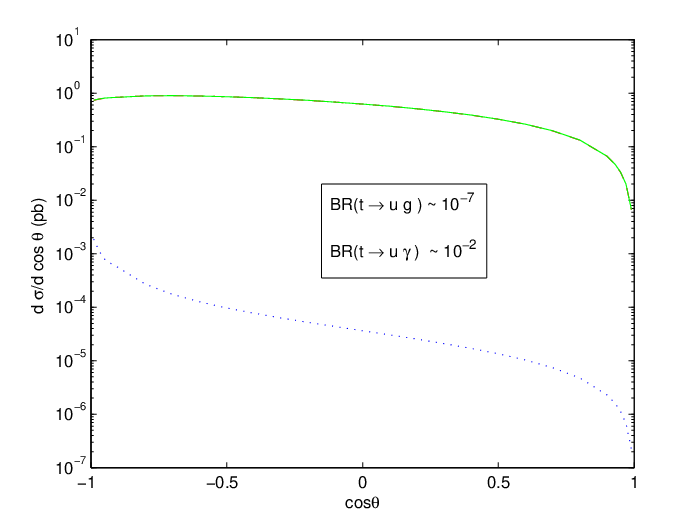
Refer to caption
Figure 3.13: Differential cross section p​p→u​g→t​γp\,p\rightarrow\,u\,g\rightarrow t\,\gamma versus cos⁡θ\cos\theta, for a typical choice of parameters with a branching ratio for t→u​gt\,\rightarrow\,u\,g much smaller than B​r​(t→u​γ)Br(t\,\rightarrow\,u\,\gamma). The electroweak contribution practically coincides with the total cross section (full line). The strong contribution is represented by the dotted line.

In fig. 3.13 we show the inverse situation: a typical set of values was chosen which gives us B​r​(t→u​γ)∼ 10−2Br(t\,\rightarrow\,u\,\gamma)\,\sim\,10^{-2} and B​r​(t→u​g)∼ 10−7Br(t\,\rightarrow\,u\,g)\,\sim\,10^{-7}, meaning a situation for which the anomalous electroweak interactions are clearly dominant over the strong ones. We see from the angular distribution of the total cross section shown in fig. 3.13 that it now greatly resembles its electroweak component. Judging from figs. 3.12 and 3.13, the telltale sign of dominance of strong FCNC interactions is a pronounced variation with cos⁡θ\cos\theta in the cross section, whereas a dominance of electroweak FCNC effects will produce a relatively “flat” cross section. The Feynman diagrams of fig. 3.7 help to explain this difference in dependence with cos⁡θ\cos\theta: the strong cross section has a significant contribution from the tt-channel (since the ss-channel diagram is suppressed by the top mass), whereas the inverse happens for the electroweak cross section. However, it should be pointed out that the four-legged diagrams contributing to both cross sections will upset a clear ss-or-tt channel dominance. Notice also that if FCNC produce branching ratios of similar size in both sectors the difference in behaviour shown in these plots will not be seen. In fact, we may get a better feel for the different angular behavior of the strong and electroweak FCNC interactions if we define an asymmetry coefficient for this cross section,

At+γ=σt+γ​(cos⁡θ>0)−σt+γ​(cos⁡θ<0)σt+γ​(cos⁡θ>0)+σt+γ​(cos⁡θ<0).A_{t+\gamma}\;=\;\frac{\sigma_{t+\gamma}(\cos\theta>0)\,-\,\sigma_{t+\gamma}(\cos\theta<0)}{\sigma_{t+\gamma}(\cos\theta>0)\,+\,\sigma_{t+\gamma}(\cos\theta<0)}\;\;\;. (3.20)

To exemplify the relevance of this quantity, we generated a special sample of anomalous couplings: random values of all strong and electroweak couplings such that B​r​(t→u​γ)+B​r​(t→u​g)∼10−2Br(t\,\rightarrow\,u\,\gamma)\,+\,Br(t\,\rightarrow\,u\,g)\sim 10^{-2}. This will include the cases where one of the branching ratios dominates over the other, and also the case where both of them have similar magnitudes. We show the results in fig. 3.14, plotting the value of At+γA_{t+\gamma} in

Refer to caption
Figure 3.14: The angular asymmetry coefficient defined in eq. (3.20) as a function of the branching ratios B​r​(t→u​γ)Br(t\,\rightarrow\,u\,\gamma) (crosses) and B​r​(t→u​g)Br(t\,\rightarrow\,u\,g) (dots).

terms of the two branching ratios whose sum is fixed to 10−210^{-2}. Looking at the far left of the plot we see that when the electroweak FCNC interactions dominate over the strong ones At+γA_{t+\gamma} tends to a value of approximately −0.85-0.85, and in the reverse situation we have At+γ∼−0.42A_{t+\gamma}\,\sim\,-0.42. However, when both branching ratios have similar sizes, At+γA_{t+\gamma} can take any value between those two limits.

3.3.2 Cross section for q​g→t​Zq\,g\rightarrow t\,Z

We can perform analysis similar to those of the previous section for the associated production of a top and a Z boson. We computed an analytical expression for the cross section of this process, which is given by the sum of three terms,

d​σq​g→t​Zd​t=d​σq​g→t​ZE​Wd​t+d​σq​g→t​ZSd​t+d​σq​g→t​ZI​n​td​t,\frac{d\sigma_{qg\rightarrow tZ}}{dt}\;=\;\frac{d\sigma^{EW}_{qg\rightarrow tZ}}{dt}\;+\;\frac{d\sigma^{S}_{qg\rightarrow tZ}}{dt}\;+\;\frac{d\sigma^{Int}_{qg\rightarrow tZ}}{dt}\;\;\;, (3.21)

with strong FCNC contributions (σS\sigma^{S}), electroweak ones (σE​W\sigma^{EW}) and interference terms between both sectors. The expression for d​σq​g→t​ZS/d​td\sigma^{S}_{qg\rightarrow tZ}/dt was first given in ref. [18]. The remaining formulae are quite lengthy, involving many different combinations of anomalous couplings with complicated coefficients. We present them in Appendix 3.A for completeness. To examine the values of these cross sections at the LHC, we used the set of anomalous couplings generated in the previous section, complemented with randomly generated values for the η\eta and θ\theta couplings 44 4 Which, recall, do not contribute to FCNC interactions involving the photon, only the Z. and integrated the expressions (3.21) with the CTEQ6M pdf’s. We chose μF=mt+mZ\mu_{F}\,=\,m_{t}\,+\,m_{Z} and imposed a 10 GeV cut on the transverse momentum of the particles in the final state.

Refer to caption
Figure 3.15: Total (electroweak and strong contributions) cross section for the process p​p→u​g→t​Zp\,p\rightarrow\,u\,g\rightarrow t\,Z versus the sum of the FCNC branching ratios for the decays t→u​Zt\,\rightarrow\,u\,Z and t→u​gt\,\rightarrow\,u\,g.

Unlike what was observed for the t​γt\,\gamma channel, there is no direct proportionality between σE​W​(p​p→u​g→t​Z)\sigma^{EW}(pp\rightarrow ug\rightarrow tZ) and B​r​(t→q​Z)Br(t\,\rightarrow\,q\,Z) – this is due to the many different functions multiplying the several combinations of anomalous couplings presented in Appendix 3.A. Because the functions F1ZF_{1_{Z}} and F2ZF_{2_{Z}} (eqs. (3.29)) are very similar, there is an approximate proportionality between the branching ratio and σS​(p​p→u​g→t​Z)\sigma^{S}(pp\rightarrow ug\rightarrow tZ), as was seen in ref. [18]. In fig. 3.15 we plot the total cross section for this process against the sum B​r​(t→u​Z)+B​r​(t→u​g)Br(t\,\rightarrow\,u\,Z)\,+\,Br(t\,\rightarrow\,u\,g). We see, from this plot, that the cross section for t+Zt\,+\,Z production is always contained between two straight lines, and it is easy to obtain the following relation, valid for the overwhelming majority of the points shown in fig. 3.15:

200​[B​r​(t→u​g)+B​r​(t→u​Z)]<σ⁡(p​p→u​g→t​Z)< 104​[B​r​(t→u​g)+B​r​(t→u​Z)]​(pb).200\,\left[Br(t\rightarrow u\,g)\,+\,Br(t\rightarrow u\,Z)\right]\,<\,\sigma(pp\rightarrow u\,g\rightarrow t\,Z)\,<\,10^{4}\,\left[Br(t\rightarrow u\,g)\,+\,Br(t\rightarrow u\,Z)\right]\,\mbox{(pb)}. (3.22)

The thick band observed in this figure means any bounds obtained, say, on the cross section, will translate into a less severe bound on the sum of the branching ratios than what happened for the t+γt\,+\,\gamma channel. For instance, in fig. 3.11 an upper bound on the cross section σ⁡(p​p→u​g→t​γ)\sigma(pp\rightarrow ug\rightarrow t\gamma) of 10−210^{-2} implied B​r​(t→u​γ)+B​r​(t→u​g)< 10−5Br(t\,\rightarrow\,u\,\gamma)\,+\,Br(t\,\rightarrow\,u\,g)\,<\,10^{-5}, whereas a similar bound on σ⁡(p​p→u​g→t​Z)\sigma(pp\rightarrow ug\rightarrow tZ) gives us approximately, from the right-hand side of the band in fig. 3.15, B​r​(t→u​Z)+B​r​(t→u​g)< 10−4Br(t\,\rightarrow\,u\,Z)\,+\,Br(t\,\rightarrow\,u\,g)\,<\,10^{-4}. If we didn’t have this band of values, but rather a line corresponding to its left-hand side edge, the bound would be one order of magnitude lower. As before, we obtain qualitatively identical results for the processes involving the cc quark, and we can quote rough bounds similar to those of eq. (3.22),

30​[B​r​(t→c​g)+B​r​(t→c​Z)]<σ⁡(p​p→c​g→t​Z)< 600​[B​r​(t→c​g)+B​r​(t→c​Z)]​(pb).30\,\left[Br(t\rightarrow c\,g)\,+\,Br(t\rightarrow c\,Z)\right]\,<\,\sigma(pp\rightarrow c\,g\rightarrow t\,Z)\,<\,600\,\left[Br(t\rightarrow c\,g)\,+\,Br(t\rightarrow c\,Z)\right]\,\mbox{(pb)}. (3.23)
Refer to caption
Figure 3.16: Differential cross sections for the process p​p→u​g→t​Zpp\rightarrow ug\rightarrow tZ. Total (thick line), electroweak (dashed line) and strong (dotted line) contributions. The electroweak contribution practically coincides with the strong one.

And again, we observe that the strong and electroweak cross sections have different angular dependencies. In fig. 3.16 we plot the differential cross section for the process p​p→u​g→t​Zpp\rightarrow ug\rightarrow tZ, both the strong and electroweak contributions, for a typical choice of anomalous couplings for which the electroweak FCNC interactions dominate over the strong ones. The strong contributions increase with cos⁡θ\cos\theta, whereas the electroweak ones decrease. If the strong FCNC couplings dominate over the electroweak ones, then the total cross section would very closely mimic the angular dependence of the dotted line in fig. 3.16. Once more, if the electroweak and strong FCNC interactions have contributions of similar magnitudes, then it will not be possible to distinguish them through this analysis. We can define an asymmetry coefficient for the t+Zt\,+\,Z process as well, namely

At+Z=σt+Z​(cos⁡θ>0)−σt+Z​(cos⁡θ<0)σt+Z​(cos⁡θ>0)+σt+Z​(cos⁡θ<0).A_{t+Z}\;=\;\frac{\sigma_{t+Z}(\cos\theta>0)\,-\,\sigma_{t+Z}(\cos\theta<0)}{\sigma_{t+Z}(\cos\theta>0)\,+\,\sigma_{t+Z}(\cos\theta<0)}\;\;\;. (3.24)

We will now use the set of anomalous couplings generated to produce fig. 3.14 and plot the evolution of At+ZA_{t+Z} with both FCNC branching ratios in fig. 3.17.

Refer to caption
Figure 3.17: The angular asymmetry coefficient At+ZA_{t+Z} as a function of the branching ratios B​r​(t→u​Z)Br(t\,\rightarrow\,u\,Z) (crosses) and B​r​(t→u​g)Br(t\,\rightarrow\,u\,g) (dots).

Again, we see a clear distinction between dominance of electroweak FCNC interactions or strong FCNC ones. In the former case At+ZA_{t+Z} tends to a value of approximately 0.40.4, and in the latter situation we have At+Z∼−0.4A_{t+Z}\,\sim\,-0.4 – this is particulary interesting since the asymmetry changes signs, going from one regime to the other. Once more, if both branching ratios have like sizes, At+ZA_{t+Z} may have any value between these two extreme.

3.3.3 Cross section for the four-fermion channels

In the following analysis we divide the four-fermions processes in two: those which don’t have the SM contribution like processes (1) to (5) in table 3.2 and processes with the SM contribution: (6) to (8). The analytical expression for the cross section for the processes (1) to (5) is given by

d​σd​t=d​σSd​t+d​σE​Wd​t+d​σI​n​td​t,\frac{d\sigma}{dt}=\frac{d\sigma^{S}}{dt}+\frac{d\sigma^{EW}}{dt}+\frac{d\sigma^{Int}}{dt}, (3.25)

where σS,\sigma^{S}, σE​W\sigma^{EW} and σI​n​t\sigma^{Int} refer to strong and electromagnetic FCNC contribution and the interference between them, respectively. The electromagnetic term is the sum of the photon and ZZ boson FCNC contribution:

d​σE​Wd​t=d​σγd​t+d​σZd​t;\frac{d\sigma^{EW}}{dt}=\frac{d\sigma^{\gamma}}{dt}+\frac{d\sigma^{Z}}{dt}; (3.26)

and the interference term is given by

d​σI​n​td​t=d​σS​γd​t+d​σS​Zd​t+d​σγ​Zd​t.\frac{d\sigma^{Int}}{dt}=\frac{d\sigma^{S\gamma}}{dt}+\frac{d\sigma^{SZ}}{dt}+\frac{d\sigma^{\gamma Z}}{dt}. (3.27)

where the superscript S​γ,S\gamma, S​ZSZ and γ​Z\gamma Z relates to the interferences: strong+photon, strong+Z and photon+Z, respectively. We present the analytical expression for those processes in the appendix 3.B. In the previous subsections we have generated values for all anomalous coupling that come out in the expression 3.25 and integrated it with CTEQ6M pdf’s to compute the cross section in the LHC. Then, we again chose μF=mt,\mu_{F}=m_{t}, imposed a 10​G​e​V10\;GeV cut on the transverse momentum and imposed that all branching ratio must be less than 10−2​p​b.10^{-2}\;pb. Now, we should add that the total cross section for p​p→t+qp\,p\rightarrow t\,+\,q the sum of both contributions: u quark and c quark.

In fig. 3.18 we plot the value of the total and strong cross section for t+qt\,+\,q production against the strong FCNC branching ratio of the top quark.

Refer to caption
Figure 3.18: Total (blue) and strong (green) p​p→t+qp\,p\rightarrow t\,+\,q FCNC cross section as function of the branching ratio B​r​(t→q​g).Br(t\,\rightarrow\,q\,g).

Here, we register a difference between contribution from strong and electroweak decay for the t+qt\,+\,q FCNC production cross section and the contribution for the t+γt\,+\,\gamma and t+Zt\,+\,Z one: the upper limit to the electroweak contribution is, in the best of cases of order of ∼10​p​b\sim 10\,pb but the strong contribution is ∼102​p​b.\sim 10^{2}\,pb. As we saw in the previous sections (t+γt\,+\,\gamma and t+Zt\,+\,Z production), the upper limit contribution of the strong and electroweak contribution were of the same order (∼102​p​b\sim 10^{2}\,pb). Now, the upper limit of the strong and electroweak contribution is about ∼10​p​b\sim 10\,pb to the strong FCNC branching ratio ∼10−3\sim 10^{-3} and then it grow until ∼102​p​b\sim 10^{2}\,pb to a branching ratio 10−2.10^{-2}. Thus, if we find a cross section bigger than 101​p​b,10^{1}\,pb, the main contribution from the strong one but the reverse of this statement is not true.

In the previous sections we have used the asymmetry studies to have a criterion to distinguish the strong and electroweak FCNC contribution to t+γt\,+\,\gamma and t+Zt\,+\,Z production. In t+qt\,+\,q FCNC production this is not possible because both the strong and the electroweak contribution have the same Feynman diagrams without any intermediate top quark.

The cross section for t+jt\,+\,j production is the sum of following cross sections: p​p→g​g→t​q¯,p\,p\rightarrow g\,g\rightarrow t\,\bar{q}, p​p→g​q→t​gp\,p\rightarrow g\,q\rightarrow t\,g [17], p​p→g​q→tp\,p\rightarrow g\,q\rightarrow t (direct top production [16]) and p​p→q​q→t​q.p\,p\rightarrow q\,q\rightarrow t\,q\penalty\ .55 5 We didn’t include contribution from processes (6) to (8) in table 3.2 because it is not expressive as we saw. In the SM, there are three possible processes to produce t+jt\,+\,j represented by the Feynman diagrams in the figs. 2.2(a), .2.2(b) and 2.2(c). With a cross section ∼257±12​p​b\sim 257\pm 12\,pb[69, 68]. In fig. 3.19 we plot the FCNC cross section of t+jt\,+\,j production against the total FCNC branching ratio.

Refer to caption
Figure 3.19: Total (blue) and strong (green) p​p→t+jp\,p\rightarrow t\,+\,j FCNC cross section as function of the branching ratio B​r​(t→q​g).Br(t\,\rightarrow\,q\,g).

First, we note that the plot 3.19 and 3.18 are very similar except that the contribution of strong FCNC cross section is bigger by a factor of ten. Thus, the upper limit to the cross section is of order of ∼103​p​b\sim 10^{3}\,pb for a strong FCNC branching ratio equal to 10−210^{-2} and it is of order of ∼102​p​b\sim 10^{2}\,pb for a strong FCNC branching ration about 10−4.10^{-4}. For large values of the strong branching ratio the number of FCNC events could be ten times larger than what is expected for the SM.

To conclude, we briefly comment processes (6) to (8) in the table 3.2. They have a contribution to the cross section of order Λ−2\Lambda^{-2} due to the interference with SM Feynman diagrams. The analytical expressions for these cross sections are given in appendix 3.B. In the analysis of those processes we separate the final state in two: with a b quark (or b¯\bar{b}) in the final state or without it. The reason for that is: first, the off-diagonal CKM matrix elements suppress final state with top quark and other quarks other than b one; finally, the b-tag technique allows one to identify a jet from the hadronization of a b quark in the final state. In fact, the contribution with a b quark is of order ∼10\sim 10 greater than the other contributions but even in this case the total contribution is less than one as was showed in the ref. [121].

3.4  Discussion and conclusions

To summarize, we employed the effective operator formalism to parameterize the effects of any theory that might have as its low-energy limit the SM. The fact that we are working in a gauge invariant formalism allowed us to find many relations between couplings and quantities which, a priori, would not be related at all. In particular we found a near-proportionality between the cross section of associated top plus photon production at the LHC and the sum of the FCNC decays of the top to a photon and a gluon. We estimated the cross sections for t+γ,t\,+\,\gamma, t+Zt\,+\,Z and t+qt\,+\,q production at the LHC and saw that, for large enough values of the top FCNC branching ratios, one might expect a significant number of events. We also concluded that, for these processes, the interplay between the strong and electroweak anomalous interactions tends to increase the values of the cross sections – the interference between both FCNC sectors is mostly constructive. Also, if the cross section of t+qt\,+\,q production is of order of 10​p​b10\,pb and bigger then we have a criterion to evaluate the dependence of this cross section and the strong FCNC branching ratio. Finally, we saw that the upper limit of the t+jt\,+\,j FCNC cross section is one order highest than the t+qt\,+\,q. This was understood due the contribution of the gluonic processes.

Despite the advantage in using the cross section for t+jt+j FCNC production due its large values, these processes do not offer a general criterion to study the individual contribution due to the strong or electroweak FCNC decay. In other words, we know the total cross section but it is not easy to distinguish the strong from the electroweak contribution. This is not matter case for the t+γt+\gamma or t+Zt+Z production cross section where we can perform such studies using the FB asymmetry, as we saw. Thus, the general problem is: even if the top quark has indeed large FCNC branching ratios – strong or electroweak ones –, which would lead to significant cross sections of associated single top production at the LHC, could those processes actually be observed? In other words, given the numerous backgrounds present at the LHC, is it possible to extract a meaningful FCNC signal from the expected data? The very thorough analysis of ref. [115] seems to indicate so. For instance, for t+Zt\,+\,Z production they identify several possible channels available to identify the FCNC signal, summarised in table 3.3.

Final State Fraction (%) Backgrounds
t​Z→(b​j​j)​(j​j)tZ\rightarrow(bjj)\,(jj) 22.2 j​j​j​j​jjjjjj
t​Z→(b​j​j)​(ν​ν¯)tZ\rightarrow(bjj)\,(\nu\bar{\nu}) 8.1 t​t¯t\bar{t}, W​tWt, Z​j​j​jZjjj
t​Z→(b​l​ν)​(j​j)tZ\rightarrow(bl\nu)\,(jj) 7.5 t​t¯t\bar{t}, W​tWt, W​j​j​jWjjj
t​Z→(b​l​ν)​(ν​ν¯)tZ\rightarrow(bl\nu)\,(\nu\bar{\nu}) 2.7 W​jWj
t​Z→(b​j​j)​(l​l)tZ\rightarrow(bjj)\,(ll) 2.3 Z​j​j​jZjjj, Z​W​jZWj
t​Z→(b​j​j)​(b¯​b)tZ\rightarrow(bjj)\,(\bar{b}b) 2.2 b​b¯​j​j​jb\bar{b}jjj
t​Z→(b​l​ν)​(l​l)tZ\rightarrow(bl\nu)\,(ll) 0.8 Z​W​jZWj
t​Z→(b​l​ν)​(b¯​b)tZ\rightarrow(bl\nu)\,(\bar{b}b) 0.7 t​t¯t\bar{t}, W​tWt, Z​W​jZWj, W​b​b¯​jWb\bar{b}j
Table 3.3: Possible final states in t​Zt\,Z production, and main backgrounds to each process [115].

For all of these processes, the processes W​Z​jWZj, t​t¯t\bar{t} and single top production will also act as backgrounds. It is also likely, considering the immense QCD backgrounds, that only those processes with at least one lepton will be possible to observe at the LHC. To build this table, the top quark was considered to decay according to SM physics, t→b​Wt\rightarrow b\,W, and the several decay possibilities within the SM of the WW and ZZ bosons give the possibilities listed therein. The fraction attributed to each channel corresponds to the percentages of each decay mode of the WW and ZZ as well as a 90 % tagging efficiency for lepton (electron or muon) tagging, and a 60 % one for each b-jet. The most impressive result of ref. [115], though, is the efficiency with which the FCNC signal is extracted from these backgrounds: they have shown that a battery of simple kinematical cuts on the observed particles is more than enough to obtain a very clear – and statistically meaningful – FCNC signal. For t+Zt\,+\,Z production they conclude that the best channel would be p​p→t​Z→l+​l−​l​ν​bp\,p\rightarrow t\,Z\rightarrow l^{+}\,l^{-}\,l\,\nu\,b. For t+γt\,+\,\gamma production the analysis is made simpler by the photon not having decay branching ratios, which aides the statistics obtained – the best channel available would be p​p→t​γ→γ​l​ν​bp\,p\rightarrow t\,\gamma\rightarrow\gamma\,l\,\nu\,b. Clearly, only an analysis analogous to that of [115], with the FCNC interactions considered in the present thesis included in an event generator, would be capable of reaching definite conclusions regarding which kinematical cuts would be better suited to obtain a clear FCNC signal. That study is beyond the scope of the present thesis, though a preliminary study of our strong FCNC interactions in the LHC environment, using the TopReX event generator [123], is about to be concluded [124]. A word on higher-order QCD corrections: they are manifestly difficult to compute in the effective operator formalism, since the Lagrangian becomes non-renormalizable. A recent work using electroweak top FCNC couplings [125], however, concluded that those corrections greatly reduce any dependence the results obtained at tree level might have on the scales of renormalization and factorization. These authors have also shown that the higher order corrections tend to slightly increase the leading order result. The analysis of the differential cross sections for t+γt\,+\,\gamma and t+Zt\,+\,Z production will possibly allow the identification of the source of FCNC physics – the strong or the electroweak sector.

Finally, we consider the process 3 in the table 3.1 i.e., t​t¯t\bar{t} production via FCNC operators. In ref. [17] the authors have calculated this cross section for the strong FCNC operator; in the appendix 3.C we present the analytical expression for this process for the electroweak FCNC operator. To obtain the cross section for the process p​p→q​q¯→t​t¯p\,p\,\rightarrow\,q\,\bar{q}\,\rightarrow\,t\,\bar{t} at the LHC we integrated the partonic cross section in eq. (3.65) in the appendix 3.C with the CTEQ6M pdf [122], with a factorization scale μF=2​mt\mu_{F}=2\,m_{t} .We also imposed a cut of 15 GeV on the pTp_{T} of the final state partons. However, it is unlikely to register such FCNC process in the LHC. By a simple inspection of the coefficients, supposing that all of coefficients are one with the same signal, the total cross section is about 20​p​b.20\,pb. The SM cross section to t​t¯t\bar{t} about 833±100​p​b833\pm 100pb [65, 63] i. e., the expected experimental error is larger then all FCNC contribution.

Appendix 3.A Cross section expression for the process q​g→t​Zq\,g\rightarrow t\,Z

As mentioned in section 3.3.2 the cross section for the associated production of a top and a Z boson is given by three terms, as in eq. (3.21). The strong FCNC contribution is given by:

d​σq​g→t​ZSd​t\displaystyle\frac{d\,\sigma^{S}_{q\,g\rightarrow t\,Z}}{dt} =e296​π​s2​Λ4{F1Z(t,s)[|αq​tS+(αt​qS)∗|2+8​vmtIm[(αq​tS+(αt​qS)∗)βt​qS]\displaystyle=\frac{e^{2}}{96\,\pi\,s^{2}\,\Lambda^{4}}\left\{F_{1_{Z}}(t,s)\,\left[\left|\alpha^{S}_{qt}+(\alpha^{S}_{tq})^{*}\right|^{2}+\frac{8v}{m_{t}}\,Im\left[(\alpha^{S}_{qt}+(\alpha^{S}_{tq})^{*})\,\beta^{S}_{tq}\right]\right.\right.
+16​v2mt2|βt​qS|2]+F2Z(t,s)16​v2mt2|βq​tS|2},\displaystyle+\left.\left.\frac{16v^{2}}{m_{t}^{2}}\,\left|\beta^{S}_{tq}\right|^{2}\right]+\,F_{2_{Z}}(t,s)\,\frac{16v^{2}}{m_{t}^{2}}\,\left|\beta^{S}_{qt}\right|^{2}\right\}\;\;\;, (3.28)

with coefficients

F1Z​(t,s)\displaystyle F_{1_{Z}}(t,s) =−mt272​cW2​mZ2​(mt2−s)2​sW2​t2\displaystyle=\frac{-m_{t}^{2}}{72\,c_{W}^{2}\,m_{Z}^{2}\,{\left(m_{t}^{2}-s\right)}^{2}\,s_{W}^{2}\,t^{2}}
×[32mt8mZ2sW4(mZ2−t)+32mt4mZ2sW4(mZ2−t)(s2+4st+t2)\displaystyle\times\left[32\,m_{t}^{8}\,m_{Z}^{2}\,s_{W}^{4}\,\left(m_{Z}^{2}-t\right)+32\,m_{t}^{4}\,m_{Z}^{2}\,s_{W}^{4}\,\left(m_{Z}^{2}-t\right)\,\left(s^{2}+4\,s\,t+t^{2}\right)\right.
+s2​t2​(2​mZ4​(9−24​sW2+32​sW4)+9​s​t−2​mZ2​(9−24​sW2+32​sW4)​(s+t))\displaystyle+s^{2}\,t^{2}\,\left(2\,m_{Z}^{4}\,\left(9-24\,s_{W}^{2}+32\,s_{W}^{4}\right)+9\,s\,t-2\,m_{Z}^{2}\,\left(9-24\,s_{W}^{2}+32\,s_{W}^{4}\right)\,\left(s+t\right)\right)\,
+mt2​s​t​(−9​s​t2−64​mZ4​sW4​(s+t)+mZ2​(32​s2​sW4+3​s​(3−32​sW2+64​sW4)​tCLOSECLOSE\displaystyle+m_{t}^{2}\,s\,t\,\left(-9\,s\,t^{2}-64\,m_{Z}^{4}\,s_{W}^{4}\,\left(s+t\right)+m_{Z}^{2}\,\left(32\,s^{2}\,s_{W}^{4}+3\,s\,\left(3-32\,s_{W}^{2}+64\,s_{W}^{4}\right)\,t\right.\right.
+96sW4t2))−32mt6mZ2sW4(2mZ2(s+t)−t(s+2t))],\displaystyle\left.\left.+96\,s_{W}^{4}\,t^{2}\right)\right)-\left.32\,m_{t}^{6}\,m_{Z}^{2}\,s_{W}^{4}\,\left(2\,m_{Z}^{2}\,\left(s+t\right)-t\,\left(s+2\,t\right)\right)\right],
F2Z​(t,s)\displaystyle F_{2_{Z}}(t,s) =mt272​cW2​mZ2​(mt2−s)2​sW2​t2{−2mt4mZ2(3−4sW2)2(mZ2−t)(s2+4st+t2)\displaystyle=\frac{m_{t}^{2}}{72\,c_{W}^{2}\,m_{Z}^{2}\,{\left(m_{t}^{2}-s\right)}^{2}\,s_{W}^{2}\,t^{2}}\left\{-2\,m_{t}^{4}\,m_{Z}^{2}\,{\left(3-4\,s_{W}^{2}\right)}^{2}\,\left(m_{Z}^{2}-t\right)\,\left(s^{2}+4\,s\,t+t^{2}\right)\right.
+s2​t2​(−2​mZ4​(9−24​sW2+32​sW4)−9​s​t+2​mZ2​(9−24​sW2+32​sW4)​(s+t))\displaystyle+s^{2}\,t^{2}\,\left(-2\,m_{Z}^{4}\,\left(9-24\,s_{W}^{2}+32\,s_{W}^{4}\right)-9\,s\,t+2\,m_{Z}^{2}\,\left(9-24\,s_{W}^{2}+32\,s_{W}^{4}\right)\,\left(s+t\right)\right)
+mt2st[9st2+4mZ4(3−4sW2)2(s+t)+mZ2(−2s2(3−4sW2)2\displaystyle+m_{t}^{2}\,s\,t\,\left[9\,s\,t^{2}+4\,m_{Z}^{4}\,{\left(3-4\,s_{W}^{2}\right)}^{2}\,\left(s+t\right)+m_{Z}^{2}\,\left(-2\,s^{2}\,{\left(3-4\,s_{W}^{2}\right)}^{2}\right.\right.
−3s(15+64(−sW2+sW4))t−6(3−4sW2)2t2)]2mt8mZ2(3−4sW2)2(−mZ2+t)\displaystyle-\left.\left.3\,s\,\left(15+64\,\left(-s_{W}^{2}+s_{W}^{4}\right)\right)\,t-6\,{\left(3-4\,s_{W}^{2}\right)}^{2}\,t^{2}\right)\right]2\,m_{t}^{8}\,m_{Z}^{2}\,{\left(3-4\,s_{W}^{2}\right)}^{2}\,\left(-m_{Z}^{2}+t\right)
+2mt6mZ2(3−4sW2)2(2mZ2(s+t)−t(s+2t))}.\displaystyle\left.+2\,m_{t}^{6}\,m_{Z}^{2}\,{\left(3-4\,s_{W}^{2}\right)}^{2}\,\left(2\,m_{Z}^{2}\,\left(s+t\right)-t\,\left(s+2\,t\right)\right)\right\}\;\;\;. (3.29)

The electroweak FCNC contribution is given by the following expression:

d​σq​g→t​ZE​Wd​t\displaystyle\frac{d\,\sigma^{EW}_{q\,g\rightarrow t\,Z}}{dt} =gs296​π​s2​Λ4[G1Z(t,s)|αq​tZ|2+G2Z(t,s)|αt​qZ|2+G3Z(t,s)(|βq​tZ|2+|βt​qZ|2)\displaystyle=\frac{g_{s}^{2}}{96\,\pi\,s^{2}\,\Lambda^{4}}\left[G_{1_{Z}}(t,s)\,\left|\alpha^{Z}_{qt}\right|^{2}+G_{2_{Z}}(t,s)\,\left|\alpha^{Z}_{tq}\right|^{2}+G_{3_{Z}}(t,s)\,(\left|\beta^{Z}_{qt}\right|^{2}+\left|\beta^{Z}_{tq}\right|^{2})\right.
+G4Z​(t,s)​(|ηq​t|2+|η¯q​t|2)+G5Z​(t,s)​|θ|2+G6Z​(t,s)​R​e​[αq​tZ​αt​qZ]\displaystyle+G_{4_{Z}}(t,s)\,(\left|\eta_{qt}\right|^{2}+\left|\bar{\eta}_{qt}\right|^{2})+\,G_{5_{Z}}(t,s)\,\left|\theta\right|^{2}+G_{6_{Z}}(t,s)\,Re\left[\alpha^{Z}_{qt}\,\alpha^{Z}_{tq}\right]
+G7Z​(t,s)​I​m​[αq​tZ​βt​qZ]+G8Z​(t,s)​I​m​[αt​qZ∗​βt​qZ]+G9Z​(t,s)​R​e​[αq​tZ​θ∗]\displaystyle+G_{7_{Z}}(t,s)\,Im\left[\alpha^{Z}_{qt}\,\beta^{Z}_{tq}\right]+\,G_{8_{Z}}(t,s)\,Im\left[\alpha^{Z^{*}}_{tq}\,\beta^{Z}_{tq}\right]+G_{9_{Z}}(t,s)\,Re\left[\alpha^{Z}_{qt}\theta^{*}\right]
+G10Z​(t,s)​R​e​[αt​qZ​θ]+G11Z​(t,s)​R​e​[βq​tZ​(ηq​t−η¯q​t)∗]\displaystyle+G_{10_{Z}}(t,s)\,Re\left[\alpha^{Z}_{tq}\theta\right]\left.+\,G_{11_{Z}}(t,s)\,Re\left[\beta^{Z}_{qt}(\eta_{qt}-\bar{\eta}_{qt})^{*}\right]\right.
+G12Z(t,s)Im[βt​qZθ]+G13Z(t,s)Re[ηq​tη¯q​t∗]]\displaystyle\left.+G_{12_{Z}}(t,s)\,Im\left[\beta^{Z}_{tq}\,\theta\right]+G_{13_{Z}}(t,s)\,Re\left[\eta_{qt}\bar{\eta}_{qt}^{*}\right]\right] (3.30)

where the GiZG_{i_{Z}} functions are given by

G1Z​(t,s)\displaystyle G_{1_{Z}}(t,s) =14​s​(mt2−t)2\displaystyle=\frac{1}{4\,s\,{\left(m_{t}^{2}-t\right)}^{2}}
×[mt10+mt8(2mZ2−2s−t)+mt6(−5mZ4+s2+4st+t2−4mZ2(s+t))\displaystyle\times\left[m_{t}^{10}+m_{t}^{8}\,\left(2\,m_{Z}^{2}-2\,s-t\right)+m_{t}^{6}\,\left(-5\,m_{Z}^{4}+s^{2}+4\,s\,t+t^{2}-4\,m_{Z}^{2}\,\left(s+t\right)\right)\right.
+mt2​(2​mZ8−8​mZ6​t−4​mZ2​t2​(s+t)+2​s​t2​(s+t)+mZ4​(s+3​t)2)\displaystyle+m_{t}^{2}\,\left(2\,m_{Z}^{8}-8\,m_{Z}^{6}\,t-4\,m_{Z}^{2}\,t^{2}\,\left(s+t\right)+2\,s\,t^{2}\,\left(s+t\right)+m_{Z}^{4}\,{\left(s+3\,t\right)}^{2}\right)
−mZ4​t​(2​mZ4+s2+t2−2​mZ2​(s+t))\displaystyle-m_{Z}^{4}\,t\,\left(2\,m_{Z}^{4}+s^{2}+t^{2}-2\,m_{Z}^{2}\,\left(s+t\right)\right)
+mt4(6mZ6−3mZ4t+2mZ2t(s+3t)−t(3s2+6st+t2))]\displaystyle\left.+m_{t}^{4}\,\left(6\,m_{Z}^{6}-3\,m_{Z}^{4}\,t+2\,m_{Z}^{2}\,t\,\left(s+3\,t\right)-t\,\left(3\,s^{2}+6\,s\,t+t^{2}\right)\right)\right]
G2Z​(t,s)\displaystyle G_{2_{Z}}(t,s) =14​s​(mt2−t)2[mt10−mt8(4mZ2+2s+t)+mt6(7mZ4+s2+2mZ2t+4st+t2)\displaystyle=\frac{1}{4\,s\,{\left(m_{t}^{2}-t\right)}^{2}}\left[m_{t}^{10}-m_{t}^{8}\,\left(4\,m_{Z}^{2}+2\,s+t\right)+m_{t}^{6}\,\left(7\,m_{Z}^{4}+s^{2}+2\,m_{Z}^{2}\,t+4\,s\,t+t^{2}\right)\right.
−mZ4​t​(2​mZ4+s2+t2−2​mZ2​(s+t))\displaystyle-m_{Z}^{4}\,t\,\left(2\,m_{Z}^{4}+s^{2}+t^{2}-2\,m_{Z}^{2}\,\left(s+t\right)\right)
−mt4​(6​mZ6+3​mZ4​t−2​mZ2​s​(s+3​t)+t⁡(3​s2+6​s​t+t2))\displaystyle-m_{t}^{4}\,\left(6\,m_{Z}^{6}+3\,m_{Z}^{4}\,t-2\,m_{Z}^{2}\,s\,\left(s+3\,t\right)+t\,\left(3\,s^{2}+6\,s\,t+t^{2}\right)\right)
+mt2(2mZ8+4mZ6t+2st2(s+t)+mZ4(s2−6st−3t2)+mZ2(−2s2t+2t3))]\displaystyle\left.+m_{t}^{2}\,\left(2\,m_{Z}^{8}+4\,m_{Z}^{6}\,t+2\,s\,t^{2}\,\left(s+t\right)+m_{Z}^{4}\,\left(s^{2}-6\,s\,t-3\,t^{2}\right)+m_{Z}^{2}\,\left(-2\,s^{2}\,t+2\,t^{3}\right)\right)\right]
G3Z​(t,s)\displaystyle G_{3_{Z}}(t,s) =2​v2s​(mt2−t)2[2mt8−mt6(3mZ2+4s+2t)\displaystyle=\frac{2\,v^{2}}{s\,{\left(m_{t}^{2}-t\right)}^{2}}\left[2\,m_{t}^{8}-m_{t}^{6}\,\left(3\,m_{Z}^{2}+4\,s+2\,t\right)\right.
−t⁡(2​mZ6−2​mZ4​(s+t)−4​s​t​(s+t)+mZ2​(s+t)2)\displaystyle-t\,\left(2\,m_{Z}^{6}-2\,m_{Z}^{4}\,\left(s+t\right)-4\,s\,t\,\left(s+t\right)+m_{Z}^{2}\,{\left(s+t\right)}^{2}\right)
+mt4​(2​mZ4−mZ2​(2​s+t)+2​(s2+4​s​t+t2))\displaystyle+m_{t}^{4}\,\left(2\,m_{Z}^{4}-m_{Z}^{2}\,\left(2\,s+t\right)+2\,\left(s^{2}+4\,s\,t+t^{2}\right)\right)
+mt2(2mZ6−4mZ4t−2t(3s2+6st+t2)+mZ2(s2+6st+5t2))]\displaystyle\left.+m_{t}^{2}\,\left(2\,m_{Z}^{6}-4\,m_{Z}^{4}\,t-2\,t\,\left(3\,s^{2}+6\,s\,t+t^{2}\right)+m_{Z}^{2}\,\left(s^{2}+6\,s\,t+5\,t^{2}\right)\right)\right]
G4Z​(t,s)\displaystyle G_{4_{Z}}(t,s) =v28​mZ2​s​(mt2−t)2[mt10−mt8(4mZ2+2s+t)+mt6(7mZ4+2mZ2t+(s+t)2)\displaystyle=\frac{v^{2}}{8\,m_{Z}^{2}\,s\,{\left(m_{t}^{2}-t\right)}^{2}}\left[m_{t}^{10}-m_{t}^{8}\,\left(4\,m_{Z}^{2}+2\,s+t\right)+m_{t}^{6}\,\left(7\,m_{Z}^{4}+2\,m_{Z}^{2}\,t+{\left(s+t\right)}^{2}\right)\right.
−mZ2​t​(2​mZ6−2​mZ4​(s+t)−4​s​t​(s+t)+mZ2​(s+t)2)\displaystyle-m_{Z}^{2}\,t\,\left(2\,m_{Z}^{6}-2\,m_{Z}^{4}\,\left(s+t\right)-4\,s\,t\,\left(s+t\right)+m_{Z}^{2}\,{\left(s+t\right)}^{2}\right)
−mt4​(6​mZ6+t​(s+t)2+mZ4​(2​s+3​t)−2​mZ2​s​(3​s+5​t))\displaystyle-m_{t}^{4}\,\left(6\,m_{Z}^{6}+t\,{\left(s+t\right)}^{2}+m_{Z}^{4}\,\left(2\,s+3\,t\right)-2\,m_{Z}^{2}\,s\,\left(3\,s+5\,t\right)\right)
+mt2mZ2(2mZ6+4mZ4t+mZ2(s2−2st−3t2)+2t(−5s2−4st+t2))]\displaystyle\left.+m_{t}^{2}\,m_{Z}^{2}\,\left(2\,m_{Z}^{6}+4\,m_{Z}^{4}\,t+m_{Z}^{2}\,\left(s^{2}-2\,s\,t-3\,t^{2}\right)+2\,t\,\left(-5\,s^{2}-4\,s\,t+t^{2}\right)\right)\right]
G5Z​(t,s)\displaystyle G_{5_{Z}}(t,s) =v42​mZ2​s​(mt2−t)2[mt8−mt6(2s+t)−2mZ2t(2mZ4+s2+t2−2mZ2(s+t))\displaystyle=\frac{v^{4}}{2\,m_{Z}^{2}\,s\,{\left(m_{t}^{2}-t\right)}^{2}}\left[m_{t}^{8}-m_{t}^{6}\,\left(2\,s+t\right)-2\,m_{Z}^{2}\,t\,\left(2\,m_{Z}^{4}+s^{2}+t^{2}-2\,m_{Z}^{2}\,\left(s+t\right)\right)\right.
+mt4​(−2​mZ4−2​mZ2​t+(s+t)2)\displaystyle+m_{t}^{4}\,\left(-2\,m_{Z}^{4}-2\,m_{Z}^{2}\,t+{\left(s+t\right)}^{2}\right)
+mt2(4mZ6−2mZ4t−t(s+t)2+2mZ2(s2−st+2t2))]\displaystyle\left.+m_{t}^{2}\,\left(4\,m_{Z}^{6}-2\,m_{Z}^{4}\,t-t\,{\left(s+t\right)}^{2}+2\,m_{Z}^{2}\,\left(s^{2}-s\,t+2\,t^{2}\right)\right)\right]
G6Z​(t,s)\displaystyle G_{6_{Z}}(t,s) =12​s​(mt2−t)2[mt10−mt8(2mZ2+2s+t)+mt6(mZ4+s2+4st+t2)\displaystyle=\frac{1}{2\,s\,{\left(m_{t}^{2}-t\right)}^{2}}\left[m_{t}^{10}-m_{t}^{8}\,\left(2\,m_{Z}^{2}+2\,s+t\right)+m_{t}^{6}\,\left(m_{Z}^{4}+s^{2}+4\,s\,t+t^{2}\right)\right.
+mZ4​t​(2​mZ4+s2+t2−2​mZ2​(s+t))−mt2​(2​mZ8+mZ4​(s−t)2−2​s​t2​(s+t))\displaystyle+m_{Z}^{4}\,t\,\left(2\,m_{Z}^{4}+s^{2}+t^{2}-2\,m_{Z}^{2}\,\left(s+t\right)\right)-m_{t}^{2}\,\left(2\,m_{Z}^{8}+m_{Z}^{4}\,{\left(s-t\right)}^{2}-2\,s\,t^{2}\,\left(s+t\right)\right)
+mt4(2mZ6−mZ4t+2mZ2t(s+t)−t(3s2+6st+t2))]\displaystyle\left.+m_{t}^{4}\,\left(2\,m_{Z}^{6}-m_{Z}^{4}\,t+2\,m_{Z}^{2}\,t\,\left(s+t\right)-t\,\left(3\,s^{2}+6\,s\,t+t^{2}\right)\right)\right]
G7Z​(t,s)\displaystyle G_{7_{Z}}(t,s) =2​mt​vs​(mt2−t)2[mt8−mt6(2s+t)+mt4(−2mZ4+s2+4st+t2−2mZ2(s+t))\displaystyle=\frac{2\,m_{t}\,v}{s\,{\left(m_{t}^{2}-t\right)}^{2}}\left[m_{t}^{8}-m_{t}^{6}\,\left(2\,s+t\right)+m_{t}^{4}\,\left(-2\,m_{Z}^{4}+s^{2}+4\,s\,t+t^{2}-2\,m_{Z}^{2}\,\left(s+t\right)\right)\right.
+2​t​(−2​mZ6+2​mZ4​(s+t)−mZ2​t​(s+t)+s​t​(s+t))\displaystyle+2\,t\,\left(-2\,m_{Z}^{6}+2\,m_{Z}^{4}\,\left(s+t\right)-m_{Z}^{2}\,t\,\left(s+t\right)+s\,t\,\left(s+t\right)\right)
+mt2(4mZ6−2mZ4t+2mZ2t(s+2t)−t(3s2+6st+t2))]\displaystyle\left.+m_{t}^{2}\,\left(4\,m_{Z}^{6}-2\,m_{Z}^{4}\,t+2\,m_{Z}^{2}\,t\,\left(s+2\,t\right)-t\,\left(3\,s^{2}+6\,s\,t+t^{2}\right)\right)\right]
G8Z​(t,s)\displaystyle G_{8_{Z}}(t,s) =2​mt​vs​(mt2−t)2[mt8−mt6(3mZ2+2s+t)+mt4(4mZ4+s2+mZ2t+4st+t2)\displaystyle=\frac{2\,m_{t}\,v}{s\,{\left(m_{t}^{2}-t\right)}^{2}}\left[m_{t}^{8}-m_{t}^{6}\,\left(3\,m_{Z}^{2}+2\,s+t\right)+m_{t}^{4}\,\left(4\,m_{Z}^{4}+s^{2}+m_{Z}^{2}\,t+4\,s\,t+t^{2}\right)\right.
+t⁡(2​mZ6−2​mZ4​(s+t)+2​s​t​(s+t)+mZ2​(−s2+t2))\displaystyle+t\,\left(2\,m_{Z}^{6}-2\,m_{Z}^{4}\,\left(s+t\right)+2\,s\,t\,\left(s+t\right)+m_{Z}^{2}\,\left(-s^{2}+t^{2}\right)\right)
−mt2(2mZ6+2mZ4t−mZ2(s2+4st+t2)+t(3s2+6st+t2))]\displaystyle\left.-m_{t}^{2}\,\left(2\,m_{Z}^{6}+2\,m_{Z}^{4}\,t-m_{Z}^{2}\,\left(s^{2}+4\,s\,t+t^{2}\right)+t\,\left(3\,s^{2}+6\,s\,t+t^{2}\right)\right)\right]
G9Z​(t,s)\displaystyle G_{9_{Z}}(t,s) =v2s​(mt2−t)2[−2mt8+mt4(−2mZ4+mZ2t−2t2)\displaystyle=\frac{v^{2}}{s\,{\left(m_{t}^{2}-t\right)}^{2}}\left[-2\,m_{t}^{8}+m_{t}^{4}\,\left(-2\,m_{Z}^{4}+m_{Z}^{2}\,t-2\,t^{2}\right)\right.
+mt6​(3​mZ2+2​(s+t))+mZ2​t​(2​mZ4+s2+t2−2​mZ2​(s+t))\displaystyle+m_{t}^{6}\,\left(3\,m_{Z}^{2}+2\,\left(s+t\right)\right)+m_{Z}^{2}\,t\,\left(2\,m_{Z}^{4}+s^{2}+t^{2}-2\,m_{Z}^{2}\,\left(s+t\right)\right)
−mt2(2mZ6−4mZ4t−2t2(s+t)+mZ2(s2+2st+5t2))]\displaystyle\left.-m_{t}^{2}\,\left(2\,m_{Z}^{6}-4\,m_{Z}^{4}\,t-2\,t^{2}\,\left(s+t\right)+m_{Z}^{2}\,\left(s^{2}+2\,s\,t+5\,t^{2}\right)\right)\right]
G10Z​(t,s)\displaystyle G_{10_{Z}}(t,s) =−v2s​(mt2−t)2[mt8−mt6(3mZ2+t)+mt4(4mZ4−s2+mZ2t−2st+t2)\displaystyle=\frac{-v^{2}}{s\,{\left(m_{t}^{2}-t\right)}^{2}}\left[m_{t}^{8}-m_{t}^{6}\,\left(3\,m_{Z}^{2}+t\right)+m_{t}^{4}\,\left(4\,m_{Z}^{4}-s^{2}+m_{Z}^{2}\,t-2\,s\,t+t^{2}\right)\right.
+mZ2​t​(2​mZ4+s2+t2−2​mZ2​(s+t))\displaystyle+m_{Z}^{2}\,t\,\left(2\,m_{Z}^{4}+s^{2}+t^{2}-2\,m_{Z}^{2}\,\left(s+t\right)\right)
−mt2(2mZ6+2mZ4t−s2t+t3+mZ2(s2−4st−t2))]\displaystyle\left.-m_{t}^{2}\,\left(2\,m_{Z}^{6}+2\,m_{Z}^{4}\,t-s^{2}\,t+t^{3}+m_{Z}^{2}\,\left(s^{2}-4\,s\,t-t^{2}\right)\right)\right]
G11Z​(t,s)\displaystyle G_{11_{Z}}(t,s) =v2s​(mt2−t)2[mt8−mt6(3mZ2−2s+t)\displaystyle=\frac{v^{2}}{s\,{\left(m_{t}^{2}-t\right)}^{2}}\left[m_{t}^{8}-m_{t}^{6}\,\left(3\,m_{Z}^{2}-2\,s+t\right)\right.
+t⁡(2​mZ6−2​mZ4​(s+t)−4​s​t​(s+t)+mZ2​(s+t)2)\displaystyle+t\,\left(2\,m_{Z}^{6}-2\,m_{Z}^{4}\,\left(s+t\right)-4\,s\,t\,\left(s+t\right)+m_{Z}^{2}\,{\left(s+t\right)}^{2}\right)
+mt4​(4​mZ4−3​s2−10​s​t+t2+mZ2​(2​s+t))\displaystyle+m_{t}^{4}\,\left(4\,m_{Z}^{4}-3\,s^{2}-10\,s\,t+t^{2}+m_{Z}^{2}\,\left(2\,s+t\right)\right)
−mt2(2mZ6+2mZ4t+mZ2(s2−t2)+t(−7s2−10st+t2))]\displaystyle\left.-m_{t}^{2}\,\left(2\,m_{Z}^{6}+2\,m_{Z}^{4}\,t+m_{Z}^{2}\,\left(s^{2}-t^{2}\right)+t\,\left(-7\,s^{2}-10\,s\,t+t^{2}\right)\right)\right]
G12Z​(t,s)\displaystyle G_{12_{Z}}(t,s) =−2​mt​v3s​(mt2−t)2[3mt6−mt4(6mZ2+2s+3t)+mt2(6mZ4−s2−2st+3t2)\displaystyle=\frac{-2\,m_{t}\,v^{3}}{s\,{\left(m_{t}^{2}-t\right)}^{2}}\,\left[3\,m_{t}^{6}-m_{t}^{4}\,\left(6\,m_{Z}^{2}+2\,s+3\,t\right)+m_{t}^{2}\,\left(6\,m_{Z}^{4}-s^{2}-2\,s\,t+3\,t^{2}\right)\right.
+t(−6mZ4+s2−2st−3t2+6mZ2(s+t))]\displaystyle+\left.t\,\left(-6\,m_{Z}^{4}+s^{2}-2\,s\,t-3\,t^{2}+6\,m_{Z}^{2}\,\left(s+t\right)\right)\right]
G13Z​(t,s)\displaystyle G_{13_{Z}}(t,s) =−v24​mZ2​s​(mt2−t)2[mt10−mt8(4mZ2+2s+t)+mt6(7mZ4+2mZ2t+(s+t)2)\displaystyle=\frac{-v^{2}}{4\,m_{Z}^{2}\,s\,{\left(m_{t}^{2}-t\right)}^{2}}\left[m_{t}^{10}-m_{t}^{8}\,\left(4\,m_{Z}^{2}+2\,s+t\right)+m_{t}^{6}\,\left(7\,m_{Z}^{4}+2\,m_{Z}^{2}\,t+{\left(s+t\right)}^{2}\right)\right.
−mZ2​t​(2​mZ6−2​mZ4​(s+t)−4​s​t​(s+t)+mZ2​(s+t)2)\displaystyle-m_{Z}^{2}\,t\,\left(2\,m_{Z}^{6}-2\,m_{Z}^{4}\,\left(s+t\right)-4\,s\,t\,\left(s+t\right)+m_{Z}^{2}\,{\left(s+t\right)}^{2}\right)
−mt4​(6​mZ6+t​(s+t)2+mZ4​(2​s+3​t)−2​mZ2​s​(3​s+5​t))\displaystyle-m_{t}^{4}\,\left(6\,m_{Z}^{6}+t\,{\left(s+t\right)}^{2}+m_{Z}^{4}\,\left(2\,s+3\,t\right)-2\,m_{Z}^{2}\,s\,\left(3\,s+5\,t\right)\right)
+mt2mZ2(2mZ6+4mZ4t+mZ2(s2−2st−3t2)+2t(−5s2−4st+t2))].\displaystyle\left.+m_{t}^{2}\,m_{Z}^{2}\,\left(2\,m_{Z}^{6}+4\,m_{Z}^{4}\,t+m_{Z}^{2}\,\left(s^{2}-2\,s\,t-3\,t^{2}\right)+2\,t\,\left(-5\,s^{2}-4\,s\,t+t^{2}\right)\right)\right]\;\;\;. (3.31)

Finally, the strong-electroweak interference cross section is given by

d​σq​g→t​ZI​n​td​t\displaystyle\frac{d\,\sigma^{Int}_{q\,g\rightarrow t\,Z}}{dt} =e​gs96​π​s2​Λ4[H1Z(t,s){Re[(αq​tS+αt​qS∗)αq​tZ∗]+4​vm​tIm[βt​qSαq​tZ]}\displaystyle=\frac{e\,g_{s}}{96\,\pi\,s^{2}\,\Lambda^{4}}\left[H_{1_{Z}}(t,s)\,\left\{Re\left[\left(\alpha^{S}_{qt}+\alpha^{S^{*}}_{tq}\right)\alpha^{Z^{*}}_{qt}\right]+\frac{4\,v}{mt}\,Im\left[\beta^{S}_{tq}\,\alpha^{Z}_{qt}\right]\right\}\right.
+H2Z​(t,s)​{R​e​[(αq​tS+αt​qS∗)​αt​qZ]+4​vm​t​I​m​[βt​qS​αt​qZ∗]}\displaystyle+H_{2_{Z}}(t,s)\,\left\{Re\left[\left(\alpha^{S}_{qt}+\alpha^{S^{*}}_{tq}\right)\alpha^{Z}_{tq}\right]+\frac{4\,v}{mt}\,Im\left[\beta^{S}_{tq}\,\alpha^{Z^{*}}_{tq}\right]\right\}
+H3Z​(t,s)​{I​m​[(αq​tS+αt​qS∗)​βt​qZ]+4​vm​t​R​e​[βt​qS∗​βt​qZ]}\displaystyle+H_{3_{Z}}(t,s)\,\left\{Im\left[\left(\alpha^{S}_{qt}+\alpha^{S^{*}}_{tq}\right)\beta^{Z}_{tq}\right]+\frac{4\,v}{mt}\,Re\left[\beta^{S^{*}}_{tq}\,\beta^{Z}_{tq}\right]\right\}
+H4Z​(t,s)​{R​e​[(αq​tS+αt​qS∗)​θ∗]+4​vm​t​I​m​[βt​qS​θ]}+H5Z​(t,s)​R​e​[βq​tS​βq​tZ∗]\displaystyle+H_{4_{Z}}(t,s)\,\left\{Re\left[\left(\alpha^{S}_{qt}+\alpha^{S^{*}}_{tq}\right)\theta^{*}\right]+\frac{4\,v}{mt}\,Im\left[\beta^{S}_{tq}\,\theta\right]\right\}+H_{5_{Z}}(t,s)\,Re\left[\beta^{S}_{qt}\,\beta^{Z^{*}}_{qt}\right]
+H6Z(t,s)Re[βq​tS(ηq​t−η¯q​t)∗]]\displaystyle\left.+H_{6_{Z}}(t,s)\,Re\left[\beta^{S}_{qt}\,\left(\eta_{qt}-\bar{\eta}_{qt}\right)^{*}\right]\right] (3.32)

with HiZH_{i_{Z}} given by

H1Z​(t,s)\displaystyle H_{1_{Z}}(t,s) =mt26​cW​(mt2−s)​sW​(mt2−t)​t\displaystyle=\frac{m_{t}^{2}}{6\,c_{W}\,\left(m_{t}^{2}-s\right)\,s_{W}\,\left(m_{t}^{2}-t\right)\,t}
[12mt6sW2t−mt4(4mZ4sW2+t(−3s+16ssW2+16sW2t))\displaystyle\left[12\,m_{t}^{6}\,s_{W}^{2}\,t-m_{t}^{4}\,\left(4\,m_{Z}^{4}\,s_{W}^{2}+t\,\left(-3\,s+16\,s\,s_{W}^{2}+16\,s_{W}^{2}\,t\right)\right)\right.
+t⁡(4​mZ4​sW2​(−s+t)+s​t​(3​s−4​s​sW2−4​sW2​t)+2​mZ2​s​(2​s​sW2−3​t+4​sW2​t))\displaystyle+t\,\left(4\,m_{Z}^{4}\,s_{W}^{2}\,\left(-s+t\right)+s\,t\,\left(3\,s-4\,s\,s_{W}^{2}-4\,s_{W}^{2}\,t\right)+2\,m_{Z}^{2}\,s\,\left(2\,s\,s_{W}^{2}-3\,t+4\,s_{W}^{2}\,t\right)\right)
+mt2​(4​mZ4​s​sW2+2​mZ2​s​(3−8​sW2)​tCLOSE\displaystyle+m_{t}^{2}\,\left(4\,m_{Z}^{4}\,s\,s_{W}^{2}+2\,m_{Z}^{2}\,s\,\left(3-8\,s_{W}^{2}\right)\,t\right.
+t(s2(−3+4sW2)+3s(−1+4sW2)t+4sW2t2))]\displaystyle\left.\left.+t\,\left(s^{2}\,\left(-3+4\,s_{W}^{2}\right)+3\,s\,\left(-1+4\,s_{W}^{2}\right)\,t+4\,s_{W}^{2}\,t^{2}\right)\right)\right]
H2Z​(t,s)\displaystyle H_{2_{Z}}(t,s) =−mt26​cW​(mt2−s)​sW​(mt2−t)​t\displaystyle=\frac{-m_{t}^{2}}{6\,c_{W}\,\left(m_{t}^{2}-s\right)\,s_{W}\,\left(m_{t}^{2}-t\right)\,t}
[t(mZ2s(4ssW2−3t)+4mZ4sW2(−s+t)+st(−3s+4ssW2+4sW2t))\displaystyle\left[t\,\left(m_{Z}^{2}\,s\,\left(4\,s\,s_{W}^{2}-3\,t\right)+4\,m_{Z}^{4}\,s_{W}^{2}\,\left(-s+t\right)+s\,t\,\left(-3\,s+4\,s\,s_{W}^{2}+4\,s_{W}^{2}\,t\right)\right)\right.
+4​mt6​sW2​(2​mZ2−3​t)+mt4​(−4​mZ4​sW2−8​mZ2​s​sW2+t⁡(−3​s+16​s​sW2+16​sW2​t))\displaystyle+4\,m_{t}^{6}\,s_{W}^{2}\,\left(2\,m_{Z}^{2}-3\,t\right)+m_{t}^{4}\,\left(-4\,m_{Z}^{4}\,s_{W}^{2}-8\,m_{Z}^{2}\,s\,s_{W}^{2}+t\,\left(-3\,s+16\,s\,s_{W}^{2}+16\,s_{W}^{2}\,t\right)\right)
+mt2​(4​mZ4​s​sW2+mZ2​t​(3​s−8​sW2​t)CLOSE\displaystyle+m_{t}^{2}\,\left(4\,m_{Z}^{4}\,s\,s_{W}^{2}+m_{Z}^{2}\,t\,\left(3\,s-8\,s_{W}^{2}\,t\right)\right.
+t(s2(3−4sW2)+3s(1−4sW2)t−4sW2t2))]\displaystyle\left.\left.+t\,\left(s^{2}\,\left(3-4\,s_{W}^{2}\right)+3\,s\,\left(1-4\,s_{W}^{2}\right)\,t-4\,s_{W}^{2}\,t^{2}\right)\right)\right]
H3Z​(t,s)\displaystyle H_{3_{Z}}(t,s) =mt​v3​cW​(mt2−s)​sW​(mt2−t)​t\displaystyle=\frac{m_{t}\,v}{3\,c_{W}\,\left(m_{t}^{2}-s\right)\,s_{W}\,\left(m_{t}^{2}-t\right)\,t}
[−8mt6sW2(mZ2−3t)+2mt4(4mZ2ssW2+t(3s−16ssW2−16sW2t))\displaystyle\left[-8\,m_{t}^{6}\,s_{W}^{2}\,\left(m_{Z}^{2}-3\,t\right)+2\,m_{t}^{4}\,\left(4\,m_{Z}^{2}\,s\,s_{W}^{2}+t\,\left(3\,s-16\,s\,s_{W}^{2}-16\,s_{W}^{2}\,t\right)\right)\right.
+s​t2​(mZ2​(−3+8​sW2)−2​(−3​s+4​s​sW2+4​sW2​t))\displaystyle+s\,t^{2}\,\left(m_{Z}^{2}\,\left(-3+8\,s_{W}^{2}\right)-2\,\left(-3\,s+4\,s\,s_{W}^{2}+4\,s_{W}^{2}\,t\right)\right)
+mt2​t​(mZ2​(s⁡(3−16​sW2)+8​sW2​t)CLOSE\displaystyle+m_{t}^{2}\,t\,\left(m_{Z}^{2}\,\left(s\,\left(3-16\,s_{W}^{2}\right)+8\,s_{W}^{2}\,t\right)\right.
+2(s2(−3+4sW2)+3s(−1+4sW2)t+4sW2t2))]\displaystyle\left.\left.+2\,\left(s^{2}\,\left(-3+4\,s_{W}^{2}\right)+3\,s\,\left(-1+4\,s_{W}^{2}\right)\,t+4\,s_{W}^{2}\,t^{2}\right)\right)\right]
H4Z​(t,s)\displaystyle H_{4_{Z}}(t,s) =−mt2​v26​cW​(mt2−s)​sW​(mt2−t)​t[8mt6sW2−8mt4(mZ2+s)sW2\displaystyle=\frac{-m_{t}^{2}\,v^{2}}{6\,c_{W}\,\left(m_{t}^{2}-s\right)\,s_{W}\,\left(m_{t}^{2}-t\right)\,t}\left[8\,m_{t}^{6}\,s_{W}^{2}-8\,m_{t}^{4}\,\left(m_{Z}^{2}+s\right)\,s_{W}^{2}\right.
+mt2​(8​mZ2​s​sW2+t⁡(9​s−16​s​sW2−8​sW2​t))\displaystyle+m_{t}^{2}\,\left(8\,m_{Z}^{2}\,s\,s_{W}^{2}+t\,\left(9\,s-16\,s\,s_{W}^{2}-8\,s_{W}^{2}\,t\right)\right)
+t(−8mZ2sW2(s−t)+s(8ssW2−9t+8sW2t))]\displaystyle\left.+t\,\left(-8\,m_{Z}^{2}\,s_{W}^{2}\,\left(s-t\right)+s\,\left(8\,s\,s_{W}^{2}-9\,t+8\,s_{W}^{2}\,t\right)\right)\right]
H5Z​(t,s)\displaystyle H_{5_{Z}}(t,s) =4​v23​cW​(mt2−s)​sW​(mt2−t)​t\displaystyle=\frac{4\,v^{2}}{3\,c_{W}\,\left(m_{t}^{2}-s\right)\,s_{W}\,\left(m_{t}^{2}-t\right)\,t}
[st2(mZ2(−3+8sW2)−2(4ssW2−3t+4sW2t))−2mt6(−3+4sW2)(mZ2−3t)\displaystyle\left[s\,t^{2}\,\left(m_{Z}^{2}\,\left(-3+8\,s_{W}^{2}\right)-2\,\left(4\,s\,s_{W}^{2}-3\,t+4\,s_{W}^{2}\,t\right)\right)-2\,m_{t}^{6}\,\left(-3+4\,s_{W}^{2}\right)\,\left(m_{Z}^{2}-3\,t\right)\right.
+2​mt4​(mZ2​s​(−3+4​sW2)+t⁡(s⁡(9−16​sW2)+4​(3−4​sW2)​t))\displaystyle+2\,m_{t}^{4}\,\left(m_{Z}^{2}\,s\,\left(-3+4\,s_{W}^{2}\right)+t\,\left(s\,\left(9-16\,s_{W}^{2}\right)+4\,\left(3-4\,s_{W}^{2}\right)\,t\right)\right)
+mt2​t​(mZ2​(s⁡(9−16​sW2)+2​(−3+4​sW2)​t)CLOSE\displaystyle+m_{t}^{2}\,t\,\left(m_{Z}^{2}\,\left(s\,\left(9-16\,s_{W}^{2}\right)+2\,\left(-3+4\,s_{W}^{2}\right)\,t\right)\right.
+2(4s2sW2+6s(−1+2sW2)t+(−3+4sW2)t2))]\displaystyle\left.\left.+2\,\left(4\,s^{2}\,s_{W}^{2}+6\,s\,\left(-1+2\,s_{W}^{2}\right)\,t+\left(-3+4\,s_{W}^{2}\right)\,t^{2}\right)\right)\right]
H6Z​(t,s)\displaystyle H_{6_{Z}}(t,s) =v23​cW​(mt2−s)​sW​(mt2−t)​t\displaystyle=\frac{v^{2}}{3\,c_{W}\,\left(m_{t}^{2}-s\right)\,s_{W}\,\left(m_{t}^{2}-t\right)\,t}
[−2mt6(−3+4sW2)(s+3t)+mt4t(s(−15+16sW2)+6(−3+4sW2)t)\displaystyle\left[-2\,m_{t}^{6}\,\left(-3+4\,s_{W}^{2}\right)\,\left(s+3\,t\right)+m_{t}^{4}\,t\,\left(s\,\left(-15+16\,s_{W}^{2}\right)+6\,\left(-3+4\,s_{W}^{2}\right)\,t\right)\right.
+mt2​t​(−6​s2+mZ2​s​(−3+8​sW2)+s⁡(15−16​sW2)​t+2​(3−4​sW2)​t2)\displaystyle+m_{t}^{2}\,t\,\left(-6\,s^{2}+m_{Z}^{2}\,s\,\left(-3+8\,s_{W}^{2}\right)+s\,\left(15-16\,s_{W}^{2}\right)\,t+2\,\left(3-4\,s_{W}^{2}\right)\,t^{2}\right)
+2mt8(−3+4sW2)+st2(mZ2(3−8sW2)+2(4ssW2+(−3+4sW2)t))].\displaystyle\left.+2\,m_{t}^{8}\,\left(-3+4\,s_{W}^{2}\right)+s\,t^{2}\,\left(m_{Z}^{2}\,\left(3-8\,s_{W}^{2}\right)+2\,\left(4\,s\,s_{W}^{2}+\left(-3+4\,s_{W}^{2}\right)\,t\right)\right)\right]\;\;\;. (3.33)

Appendix 3.B Cross section expression for the four-fermion FCNC production process

The cross section for the four-fermion channel is given by the eq. (3.25) and by the definition (3.26) and (3.27). Now, we present each term according with the anomalous decay fot the process (1), (2), (3) and (6) in table 3.2. The strong FCNC contribution is given by:

Process (1)

d​σSd​t\displaystyle\frac{d\sigma^{S}}{dt} =g32216​π​t​u​s2​Λ4{F1×|αu​tS|2+F2×|αt​uS|2+F3×[|βu​tS|2+|βt​uS|2]\displaystyle=\frac{g_{3}^{2}}{216\,\pi\,t\,u\,s^{2}\,\Lambda^{4}}\biggl\{F_{1}\times|\alpha^{S}_{ut}|^{2}+\,F_{2}\times|\alpha^{S}_{tu}|^{2}\,+\,F_{3}\times\Bigl[|\beta^{S}_{ut}|^{2}\,+\,|\beta^{S}_{tu}|^{2}\Bigr]
+F4×Re(αu​tSαt​uS)+F5×Im(αu​tSβt​uS)+F6×Im(αt​uSβt​uS∗)}\displaystyle+\,F_{4}\times Re(\alpha^{S}_{ut}\,\alpha^{S}_{tu})\,+\,F_{5}\times Im(\alpha^{S}_{ut}\,\beta^{S}_{tu})\,+\,F_{6}\times Im(\alpha^{S}_{tu}\,\beta^{S*}_{tu})\biggr\} (3.34)

with coefficients

F1\displaystyle F_{1} =−3​mt6​(t+u)+6​mt4​(t2+u2)+t​u​(7​t2+8​t​u+7​u2)\displaystyle=-3\,{m_{t}}^{6}\,\left(t+u\right)+6\,{m_{t}}^{4}\,\left(t^{2}+u^{2}\right)+t\,u\,\left(7\,t^{2}+8\,t\,u+7\,u^{2}\right)
−mt2​(6​t3+13​t2​u+13​t​u2+6​u3)\displaystyle-{m_{t}}^{2}\,\left(6\,t^{3}+13\,t^{2}\,u+13\,t\,u^{2}+6\,u^{3}\right)
F2\displaystyle F_{2} =−3​mt6​(t+u)+mt4​(6​t2+16​t​u+6​u2)+t​u​(7​t2+8​t​u+7​u2)\displaystyle=-3\,{m_{t}}^{6}\,\left(t+u\right)+{m_{t}}^{4}\,\left(6\,t^{2}+16\,t\,u+6\,u^{2}\right)+t\,u\,\left(7\,t^{2}+8\,t\,u+7\,u^{2}\right)
−mt2​(6​t3+17​t2​u+17​t​u2+6​u3)\displaystyle-{m_{t}}^{2}\,\left(6\,t^{3}+17\,t^{2}\,u+17\,t\,u^{2}+6\,u^{3}\right)
F3\displaystyle F_{3} =−16​(3​mt4​(t+u)−2​mt2​(3​t2+4​t​u+3​u2)+2​(3​t3+4​t2​u+4​t​u2+3​u3))​v2\displaystyle=-16\,\left(3\,{m_{t}}^{4}\,\left(t+u\right)-2\,{m_{t}}^{2}\,\left(3\,t^{2}+4\,t\,u+3\,u^{2}\right)+2\,\left(3\,t^{3}+4\,t^{2}\,u+4\,t\,u^{2}+3\,u^{3}\right)\right)\,v^{2}
F4\displaystyle F_{4} =−2​(3​mt6​(t+u)−2​mt4​(3​t2+4​t​u+3​u2)+t​u​(7​t2+8​t​u+7​u2)CLOSE\displaystyle=-2\,\left(3\,{m_{t}}^{6}\,\left(t+u\right)-2\,{m_{t}}^{4}\,\left(3\,t^{2}+4\,t\,u+3\,u^{2}\right)+t\,u\,\left(7\,t^{2}+8\,t\,u+7\,u^{2}\right)\right.
OPEN+mt2​(6​t3+t2​u+t​u2+6​u3))\displaystyle\left.+{m_{t}}^{2}\,\left(6\,t^{3}+t^{2}\,u+t\,u^{2}+6\,u^{3}\right)\right)
F5\displaystyle F_{5} =−8​mt​(6​t3+7​t2​u+7​t​u2+6​u3+3​mt4​(t+u)−2​mt2​(3​t2+2​t​u+3​u2))​v\displaystyle=-8\,m_{t}\,\left(6\,t^{3}+7\,t^{2}\,u+7\,t\,u^{2}+6\,u^{3}+3\,{m_{t}}^{4}\,\left(t+u\right)-2\,{m_{t}}^{2}\,\left(3\,t^{2}+2\,t\,u+3\,u^{2}\right)\right)\,v
F6\displaystyle F_{6} =24​mt​(t+u)​(mt4+2​t2+t​u+2​u2−2​mt2​(t+u))​v\displaystyle=24\,m_{t}\,\left(t+u\right)\,\left({m_{t}}^{4}+2\,t^{2}+t\,u+2\,u^{2}-2\,{m_{t}}^{2}\,\left(t+u\right)\right)\,v (3.35)

where s,t,s,t, and uu are mandelstan variable and the mtm_{t} the top quark mass.

Process (2)

d​σSd​t\displaystyle\frac{d\sigma^{S}}{dt} =g3272​π​t​s2​Λ4{F1×|αu​tS|2+F2×|αt​uS|2+F3×[|βu​tS|2+|βt​uS|2]\displaystyle=\frac{g_{3}^{2}}{72\,\pi\,t\,s^{2}\,\Lambda^{4}}\biggl\{F_{1}\times|\alpha^{S}_{ut}|^{2}+\,F_{2}\times|\alpha^{S}_{tu}|^{2}\,+\,F_{3}\times\Bigl[|\beta^{S}_{ut}|^{2}\,+\,|\beta^{S}_{tu}|^{2}\Bigr]
+F4×Re(αu​tSαt​uS)+F5×Im(αu​tSβt​uS)+F6×Im(αt​uSβt​uS∗)}\displaystyle+\,F_{4}\times Re(\alpha^{S}_{ut}\,\alpha^{S}_{tu})\,+\,F_{5}\times Im(\alpha^{S}_{ut}\,\beta^{S}_{tu})\,+\,F_{6}\times Im(\alpha^{S}_{tu}\,\beta^{S*}_{tu})\biggr\} (3.36)

with coefficients

F1\displaystyle F_{1} =−((mt2−t)​(4​mt4+s2+u2−4​mt2​(s+u)))\displaystyle=-\left(\left({m_{t}}^{2}-t\right)\,\left(4\,{m_{t}}^{4}+s^{2}+u^{2}-4\,{m_{t}}^{2}\,\left(s+u\right)\right)\right)
F2\displaystyle F_{2} =−((mt2−t)​(s2+u2))\displaystyle=-\left(\left({m_{t}}^{2}-t\right)\,\left(s^{2}+u^{2}\right)\right)
F3\displaystyle F_{3} =−16​(−2​s​u+mt2​(s+u))​v2\displaystyle=-16\,\left(-2\,s\,u+{m_{t}}^{2}\,\left(s+u\right)\right)\,v^{2}
F4\displaystyle F_{4} =−2​(mt2+t)​(s2+u2)\displaystyle=-2\,\left({m_{t}}^{2}+t\right)\,\left(s^{2}+u^{2}\right)
F5\displaystyle F_{5} =−8​mt​(mt4−t2−2​mt2​u+2​t​u+2​u2)​v\displaystyle=-8\,m_{t}\,\left({m_{t}}^{4}-t^{2}-2\,{m_{t}}^{2}\,u+2\,t\,u+2\,u^{2}\right)\,v
F6\displaystyle F_{6} =8​mt​(s2+u2)​v\displaystyle=8\,m_{t}\,\left(s^{2}+u^{2}\right)\,v (3.37)

Process (3)

d​σSd​t\displaystyle\frac{d\sigma^{S}}{dt} =g32216​π​t​s3​Λ4{F1×|αu​tS|2+F2×|αt​uS|2+F3×[|βu​tS|2+|βt​uS|2]\displaystyle=\frac{g_{3}^{2}}{216\,\pi\,t\,s^{3}\,\Lambda^{4}}\biggl\{F_{1}\times|\alpha^{S}_{ut}|^{2}+\,F_{2}\times|\alpha^{S}_{tu}|^{2}\,+\,F_{3}\times\Bigl[|\beta^{S}_{ut}|^{2}\,+\,|\beta^{S}_{tu}|^{2}\Bigr]
+F4×Re(αu​tSαt​uS)+F5×Im(αu​tSβt​uS)+F6×Im(αt​uSβt​uS∗)}\displaystyle+\,F_{4}\times Re(\alpha^{S}_{ut}\,\alpha^{S}_{tu})\,+\,F_{5}\times Im(\alpha^{S}_{ut}\,\beta^{S}_{tu})\,+\,F_{6}\times Im(\alpha^{S}_{tu}\,\beta^{S*}_{tu})\biggr\} (3.38)

with coefficients

F1\displaystyle F_{1} =6​mt4​(s−t)2−3​mt6​(s+t)+s​t​(11​s2+16​s​t+11​t2)\displaystyle=6\,{m_{t}}^{4}\,{\left(s-t\right)}^{2}-3\,{m_{t}}^{6}\,\left(s+t\right)+s\,t\,\left(11\,s^{2}+16\,s\,t+11\,t^{2}\right)
−mt2​(6​s3+5​s2​t+5​s​t2+6​t3)\displaystyle-{m_{t}}^{2}\,\left(6\,s^{3}+5\,s^{2}\,t+5\,s\,t^{2}+6\,t^{3}\right)
F2\displaystyle F_{2} =−3​mt6​(s+t)+mt4​(6​s2+20​s​t+6​t2)+s​t​(11​s2+16​s​t+11​t2)\displaystyle=-3\,{m_{t}}^{6}\,\left(s+t\right)+{m_{t}}^{4}\,\left(6\,s^{2}+20\,s\,t+6\,t^{2}\right)+s\,t\,\left(11\,s^{2}+16\,s\,t+11\,t^{2}\right)
−mt2​(6​s3+25​s2​t+25​s​t2+6​t3)\displaystyle-{m_{t}}^{2}\,\left(6\,s^{3}+25\,s^{2}\,t+25\,s\,t^{2}+6\,t^{3}\right)
F3\displaystyle F_{3} =−16​(3​mt6−3​mt4​(2​t+3​u)−2​u​(7​t2+7​t​u+3​u2)CLOSE\displaystyle=-16\,\left(3\,{m_{t}}^{6}-3\,{m_{t}}^{4}\,\left(2\,t+3\,u\right)-2\,u\,\left(7\,t^{2}+7\,t\,u+3\,u^{2}\right)\right.
OPEN+2​mt2​(3​t2+10​t​u+6​u2))​v2\displaystyle\left.+2\,{m_{t}}^{2}\,\left(3\,t^{2}+10\,t\,u+6\,u^{2}\right)\right)\,v^{2}
F4\displaystyle F_{4} =−2​(3​mt6​(s+t)−2​mt4​(3​s2+2​s​t+3​t2)+s​t​(11​s2+16​s​t+11​t2)CLOSE\displaystyle=-2\,\left(3\,{m_{t}}^{6}\,\left(s+t\right)-2\,{m_{t}}^{4}\,\left(3\,s^{2}+2\,s\,t+3\,t^{2}\right)+s\,t\,\left(11\,s^{2}+16\,s\,t+11\,t^{2}\right)\right.
OPEN+mt2​(6​s3−7​s2​t−7​s​t2+6​t3))\displaystyle\left.+{m_{t}}^{2}\,\left(6\,s^{3}-7\,s^{2}\,t-7\,s\,t^{2}+6\,t^{3}\right)\right)
F5\displaystyle F_{5} =−8​mt​(3​mt6−3​mt4​(t+3​u)−u⁡(19​t2+19​t​u+6​u2)CLOSE\displaystyle=-8\,m_{t}\,\left(3\,{m_{t}}^{6}-3\,{m_{t}}^{4}\,\left(t+3\,u\right)-u\,\left(19\,t^{2}+19\,t\,u+6\,u^{2}\right)\right.
OPEN+mt2​(3​t2+22​t​u+12​u2))​v\displaystyle\left.+{m_{t}}^{2}\,\left(3\,t^{2}+22\,t\,u+12\,u^{2}\right)\right)\,v
F6\displaystyle F_{6} =24​mt​(mt2−u)​(mt4+3​t2+3​t​u+2​u2−mt2​(3​t+2​u))​v\displaystyle=24\,m_{t}\,\left({m_{t}}^{2}-u\right)\,\left({m_{t}}^{4}+3\,t^{2}+3\,t\,u+2\,u^{2}-{m_{t}}^{2}\,\left(3\,t+2\,u\right)\right)\,v (3.39)

The electroweak (photon) FCNC contribution is given by

Process (1)

d​σγd​t\displaystyle\frac{d\sigma^{\gamma}}{dt} =e2216​π​t​u​s2​Λ4{G1×|αu​tγ|2+G2×|αt​uγ|2+G3×[|βu​tγ|2+|βt​uγ|2]\displaystyle=\frac{e^{2}}{216\,\pi\,t\,u\,s^{2}\,\Lambda^{4}}\biggl\{G_{1}\times|\alpha^{\gamma}_{ut}|^{2}+\,G_{2}\times|\alpha^{\gamma}_{tu}|^{2}\,+\,G_{3}\times\Bigl[|\beta^{\gamma}_{ut}|^{2}\,+\,|\beta^{\gamma}_{tu}|^{2}\Bigr]
+G4×Re(αu​tγαt​uγ)+G5×Im(αu​tγβt​uγ)+G6×Im(αt​uγβt​uγ∗)}\displaystyle+\,G_{4}\times Re(\alpha^{\gamma}_{ut}\,\alpha^{\gamma}_{tu})\,+\,G_{5}\times Im(\alpha^{\gamma}_{ut}\,\beta^{\gamma}_{tu})\,+\,G_{6}\times Im(\alpha^{\gamma}_{tu}\,\beta^{\gamma*}_{tu})\biggr\} (3.40)

with coefficients

G1\displaystyle G_{1} =6​mt4​(t−u)2−3​mt6​(t+u)+t​u​(11​t2+16​t​u+11​u2)\displaystyle=6\,{m_{t}}^{4}\,{\left(t-u\right)}^{2}-3\,{m_{t}}^{6}\,\left(t+u\right)+t\,u\,\left(11\,t^{2}+16\,t\,u+11\,u^{2}\right)
−mt2​(6​t3+5​t2​u+5​t​u2+6​u3)\displaystyle-{m_{t}}^{2}\,\left(6\,t^{3}+5\,t^{2}\,u+5\,t\,u^{2}+6\,u^{3}\right)
G2\displaystyle G_{2} =−3​mt6​(t+u)+mt4​(6​t2+20​t​u+6​u2)+t​u​(11​t2+16​t​u+11​u2)\displaystyle=-3\,{m_{t}}^{6}\,\left(t+u\right)+{m_{t}}^{4}\,\left(6\,t^{2}+20\,t\,u+6\,u^{2}\right)+t\,u\,\left(11\,t^{2}+16\,t\,u+11\,u^{2}\right)
−mt2​(6​t3+25​t2​u+25​t​u2+6​u3)\displaystyle-{m_{t}}^{2}\,\left(6\,t^{3}+25\,t^{2}\,u+25\,t\,u^{2}+6\,u^{3}\right)
G3\displaystyle G_{3} =−16​(6​t3+4​t2​u+4​t​u2+6​u3+3​mt4​(t+u)−2​mt2​(3​t2+2​t​u+3​u2))​v2\displaystyle=-16\,\left(6\,t^{3}+4\,t^{2}\,u+4\,t\,u^{2}+6\,u^{3}+3\,{m_{t}}^{4}\,\left(t+u\right)-2\,{m_{t}}^{2}\,\left(3\,t^{2}+2\,t\,u+3\,u^{2}\right)\right)\,v^{2}
G4\displaystyle G_{4} =−2​(3​mt6​(t+u)−2​mt4​(3​t2+2​t​u+3​u2)+t​u​(11​t2+16​t​u+11​u2)CLOSE\displaystyle=-2\,\left(3\,{m_{t}}^{6}\,\left(t+u\right)-2\,{m_{t}}^{4}\,\left(3\,t^{2}+2\,t\,u+3\,u^{2}\right)+t\,u\,\left(11\,t^{2}+16\,t\,u+11\,u^{2}\right)\right.
OPEN+mt2​(6​t3−7​t2​u−7​t​u2+6​u3))\displaystyle\left.+{m_{t}}^{2}\,\left(6\,t^{3}-7\,t^{2}\,u-7\,t\,u^{2}+6\,u^{3}\right)\right)
G5\displaystyle G_{5} =−8​mt​(6​t3−t2​u−t​u2+6​u3+3​mt4​(t+u)+mt2​(−6​t2+4​t​u−6​u2))​v\displaystyle=-8\,m_{t}\,\left(6\,t^{3}-t^{2}\,u-t\,u^{2}+6\,u^{3}+3\,{m_{t}}^{4}\,\left(t+u\right)+{m_{t}}^{2}\,\left(-6\,t^{2}+4\,t\,u-6\,u^{2}\right)\right)\,v
G6\displaystyle G_{6} =24​mt​(t+u)​(mt4+2​t2+t​u+2​u2−2​mt2​(t+u))​v\displaystyle=24\,m_{t}\,\left(t+u\right)\,\left({m_{t}}^{4}+2\,t^{2}+t\,u+2\,u^{2}-2\,{m_{t}}^{2}\,\left(t+u\right)\right)\,v (3.41)

Process (2)

d​σγd​t\displaystyle\frac{d\sigma^{\gamma}}{dt} =e272​π​t​s2​Λ4{G1×|αu​tγ|2+G2×|αt​uγ|2+G3×[|βu​tγ|2+|βt​uγ|2]\displaystyle=\frac{e^{2}}{72\,\pi\,t\,s^{2}\,\Lambda^{4}}\biggl\{G_{1}\times|\alpha^{\gamma}_{ut}|^{2}+\,G_{2}\times|\alpha^{\gamma}_{tu}|^{2}\,+\,G_{3}\times\Bigl[|\beta^{\gamma}_{ut}|^{2}\,+\,|\beta^{\gamma}_{tu}|^{2}\Bigr]
+G4×Re(αu​tγαt​uγ)+G5×Im(αu​tγβt​uγ)+G6×Im(αt​uγβt​uγ∗)}\displaystyle+\,G_{4}\times Re(\alpha^{\gamma}_{ut}\,\alpha^{\gamma}_{tu})\,+\,G_{5}\times Im(\alpha^{\gamma}_{ut}\,\beta^{\gamma}_{tu})\,+\,G_{6}\times Im(\alpha^{\gamma}_{tu}\,\beta^{\gamma*}_{tu})\biggr\} (3.42)

with coefficients

G1\displaystyle G_{1} =−((mt2−t)​(4​mt4+s2+u2−4​mt2​(s+u)))\displaystyle=-\left(\left({m_{t}}^{2}-t\right)\,\left(4\,{m_{t}}^{4}+s^{2}+u^{2}-4\,{m_{t}}^{2}\,\left(s+u\right)\right)\right)
G2\displaystyle G_{2} =−((mt2−t)​(s2+u2))\displaystyle=-\left(\left({m_{t}}^{2}-t\right)\,\left(s^{2}+u^{2}\right)\right)
G3\displaystyle G_{3} =−16​(−2​s​u+mt2​(s+u))​v2\displaystyle=-16\,\left(-2\,s\,u+{m_{t}}^{2}\,\left(s+u\right)\right)\,v^{2}
G4\displaystyle G_{4} =−2​(mt2+t)​(s2+u2)\displaystyle=-2\,\left({m_{t}}^{2}+t\right)\,\left(s^{2}+u^{2}\right)
G5\displaystyle G_{5} =−8​mt​(mt4−t2−2​mt2​u+2​t​u+2​u2)​v\displaystyle=-8\,m_{t}\,\left({m_{t}}^{4}-t^{2}-2\,{m_{t}}^{2}\,u+2\,t\,u+2\,u^{2}\right)\,v
G6\displaystyle G_{6} =8​mt​(s2+u2)​v\displaystyle=8\,m_{t}\,\left(s^{2}+u^{2}\right)\,v (3.43)

Process (3)

d​σγd​t\displaystyle\frac{d\sigma^{\gamma}}{dt} =e2216​π​t​s3​Λ4{G1×|αu​tγ|2+G2×|αt​uγ|2+G3×[|βu​tγ|2+|βt​uγ|2]\displaystyle=\frac{e^{2}}{216\,\pi\,t\,s^{3}\,\Lambda^{4}}\biggl\{G_{1}\times|\alpha^{\gamma}_{ut}|^{2}+\,G_{2}\times|\alpha^{\gamma}_{tu}|^{2}\,+\,G_{3}\times\Bigl[|\beta^{\gamma}_{ut}|^{2}\,+\,|\beta^{\gamma}_{tu}|^{2}\Bigr]
+G4×Re(αu​tγαt​uγ)+G5×Im(αu​tγβt​uγ)+G6×Im(αt​uγβt​uγ∗)}\displaystyle+\,G_{4}\times Re(\alpha^{\gamma}_{ut}\,\alpha^{\gamma}_{tu})\,+\,G_{5}\times Im(\alpha^{\gamma}_{ut}\,\beta^{\gamma}_{tu})\,+\,G_{6}\times Im(\alpha^{\gamma}_{tu}\,\beta^{\gamma*}_{tu})\biggr\} (3.44)

with coefficients

G1\displaystyle G_{1} =−3​mt6​(s+t)+6​mt4​(s2+t2)+s​t​(7​s2+8​s​t+7​t2)\displaystyle=-3\,{m_{t}}^{6}\,\left(s+t\right)+6\,{m_{t}}^{4}\,\left(s^{2}+t^{2}\right)+s\,t\,\left(7\,s^{2}+8\,s\,t+7\,t^{2}\right)
−mt2​(6​s3+13​s2​t+13​s​t2+6​t3)\displaystyle-{m_{t}}^{2}\,\left(6\,s^{3}+13\,s^{2}\,t+13\,s\,t^{2}+6\,t^{3}\right)
G2\displaystyle G_{2} =−3​mt6​(s+t)+mt4​(6​s2+16​s​t+6​t2)+s​t​(7​s2+8​s​t+7​t2)\displaystyle=-3\,{m_{t}}^{6}\,\left(s+t\right)+{m_{t}}^{4}\,\left(6\,s^{2}+16\,s\,t+6\,t^{2}\right)+s\,t\,\left(7\,s^{2}+8\,s\,t+7\,t^{2}\right)
−mt2​(6​s3+17​s2​t+17​s​t2+6​t3)\displaystyle-{m_{t}}^{2}\,\left(6\,s^{3}+17\,s^{2}\,t+17\,s\,t^{2}+6\,t^{3}\right)
G3\displaystyle G_{3} =−16​(3​mt6−3​mt4​(2​t+3​u)−2​u​(5​t2+5​t​u+3​u2)CLOSE\displaystyle=-16\,\left(3\,{m_{t}}^{6}-3\,{m_{t}}^{4}\,\left(2\,t+3\,u\right)-2\,u\,\left(5\,t^{2}+5\,t\,u+3\,u^{2}\right)\right.
OPEN+2​mt2​(3​t2+8​t​u+6​u2))​v2\displaystyle\left.+2\,{m_{t}}^{2}\,\left(3\,t^{2}+8\,t\,u+6\,u^{2}\right)\right)\,v^{2}
G4\displaystyle G_{4} =−2​(3​mt6​(s+t)−2​mt4​(3​s2+4​s​t+3​t2)+s​t​(7​s2+8​s​t+7​t2)CLOSE\displaystyle=-2\,\left(3\,{m_{t}}^{6}\,\left(s+t\right)-2\,{m_{t}}^{4}\,\left(3\,s^{2}+4\,s\,t+3\,t^{2}\right)+s\,t\,\left(7\,s^{2}+8\,s\,t+7\,t^{2}\right)\right.
OPEN+mt2​(6​s3+s2​t+s​t2+6​t3))\displaystyle\left.+{m_{t}}^{2}\,\left(6\,s^{3}+s^{2}\,t+s\,t^{2}+6\,t^{3}\right)\right)
G5\displaystyle G_{5} =−8​mt​(3​mt6−3​mt4​(t+3​u)−u⁡(11​t2+11​t​u+6​u2)CLOSE\displaystyle=-8\,m_{t}\,\left(3\,{m_{t}}^{6}-3\,{m_{t}}^{4}\,\left(t+3\,u\right)-u\,\left(11\,t^{2}+11\,t\,u+6\,u^{2}\right)\right.
OPEN+mt2​(3​t2+14​t​u+12​u2))​v\displaystyle\left.+{m_{t}}^{2}\,\left(3\,t^{2}+14\,t\,u+12\,u^{2}\right)\right)\,v
G6\displaystyle G_{6} =24​mt​(mt2−u)​(mt4+3​t2+3​t​u+2​u2−mt2​(3​t+2​u))​v\displaystyle=24\,m_{t}\,\left({m_{t}}^{2}-u\right)\,\left({m_{t}}^{4}+3\,t^{2}+3\,t\,u+2\,u^{2}-{m_{t}}^{2}\,\left(3\,t+2\,u\right)\right)\,v (3.45)

The electroweak (Z boson) FCNC contribution is given by the following expression

Process (1)

d​σZd​t\displaystyle\frac{d\sigma^{Z}}{dt} =e262208​π​Cw​Sw​(mZ2−t)2​(mZ2−u)2​s2​Λ4{H1|αu​tZ|2+H2|αt​uZ|2+H3|βu​tZ|2]\displaystyle=\frac{e^{2}}{62208\,\pi\,C_{w}\,S_{w}\,(m_{Z}^{2}-t)^{2}\,(m_{Z}^{2}-u)^{2}\,s^{2}\,\Lambda^{4}}\biggl\{H_{1}\,|\alpha^{Z}_{ut}|^{2}+\,H_{2}\,|\alpha^{Z}_{tu}|^{2}\,+\,H_{3}\,|\beta^{Z}_{ut}|^{2}\,\Bigr]
+H4​|βt​uZ|2+H5​[|η|2+|η¯|2−2​R​e​(η​η¯∗)]+H6​|θ|2+H7​R​e​(αu​tZ​αt​uZ)\displaystyle+\,H_{4}\,|\beta^{Z}_{tu}|^{2}\,+\,H_{5}\,\Bigl[|\eta|^{2}\,+\,|\bar{\eta}|^{2}\,-2\,Re(\eta\,\bar{\eta}^{*})\Bigr]\,+\,H_{6}\,|\theta|^{2}+\,H_{7}\,Re(\alpha^{Z}_{ut}\,\alpha^{Z}_{tu})
+H8Im(αu​tZβt​uZ)+H9Re(αu​tZθ∗)+H10Im(αt​uZβt​uZ∗)+H11Re(αt​uZθ)\displaystyle+H_{8}\,Im(\alpha^{Z}_{ut}\,\beta^{Z}_{tu})\,+\,H_{9}\,Re(\alpha^{Z}_{ut}\,\theta^{*})\,+\,H_{10}\,Im(\alpha^{Z}_{tu}\,\beta^{Z*}_{tu})\,+\,H_{11}\,Re(\alpha^{Z}_{tu}\,\theta)
+H12[Re(βu​tZη∗)−Re(βu​tZη¯∗)]+H13Im(βt​uZθ)}\displaystyle+\,H_{12}\Bigl[Re(\beta^{Z}_{ut}\,\eta^{*})\,-\,Re(\beta^{Z}_{ut}\,\bar{\eta}^{*})\Bigr]\,+\,H_{13}\,Im(\beta^{Z}_{tu}\,\theta)\biggr\} (3.46)

with coefficients

H1\displaystyle H_{1} OPEN=−192​mt4​Sw4​(t−u)2​(mZ4−2​t​u)+t2​u2​((243−432​Sw2+704​Sw4)​t2))+1024​Sw4​t​u\displaystyle=-192\,{m_{t}}^{4}\,{S_{w}}^{4}\,{(t-u)}^{2}\,({m_{Z}}^{4}-2\,t\,u)+t^{2}\,u^{2}\,((243-432\,{S_{w}}^{2}+704\,{S_{w}}^{4})\,t^{2}))+1024\,{S_{w}}^{4}\,t\,u
OPEN+(243−432​Sw2+704​Sw4)​u2)−192​mt6​Sw4​(−4​mZ2​t​u+mZ4​(t+u)+t​u​(t+u))\displaystyle+(243-432\,{S_{w}}^{2}+704\,{S_{w}}^{4})\,u^{2})-192\,{m_{t}}^{6}\,{S_{w}}^{4}\,(-4\,{m_{Z}}^{2}\,t\,u+{m_{Z}}^{4}\,(t+u)+t\,u\,(t+u))
−2​mZ2​t​u​(243​t​u​(t+u)−432​Sw2​t​u​(t+u)+64​Sw4​(4​t3+15​t2​u+15​t​u2+4​u3))\displaystyle-2\,{m_{Z}}^{2}\,t\,u\,(243\,t\,u\,(t+u)-432\,{S_{w}}^{2}\,t\,u\,(t+u)+64\,{S_{w}}^{4}\,(4\,t^{3}+15\,t^{2}\,u+15\,t\,u^{2}+4\,u^{3}))
+2​mZ4​(243​t2​u2−432​Sw2​t2​u2+32​Sw4​(3​t4+8​t3​u+16​t2​u2+8​t​u3+3​u4))\displaystyle+2\,{m_{Z}}^{4}\,(243\,t^{2}\,u^{2}-432\,{S_{w}}^{2}\,t^{2}\,u^{2}+32\,{S_{w}}^{4}\,(3\,t^{4}+8\,t^{3}\,u+16\,t^{2}\,u^{2}+8\,t\,u^{3}+3\,u^{4}))
+mt2​(2​mZ2​t​u​((243−432​Sw2+64​Sw4)​t2+8​(243−432​Sw2+160​Sw4)​t​uCLOSECLOSE\displaystyle+{m_{t}}^{2}\,(2\,{m_{Z}}^{2}\,t\,u\,((243-432\,{S_{w}}^{2}+64\,{S_{w}}^{4})\,t^{2}+8\,(243-432\,{S_{w}}^{2}+160\,{S_{w}}^{4})\,t\,u
OPEN+(243−432​Sw2+64​Sw4)​u2)−t​u​((243−432​Sw2+384​Sw4)​t3CLOSE\displaystyle+(243-432\,{S_{w}}^{2}+64\,{S_{w}}^{4})\,u^{2})-t\,u\,((243-432\,{S_{w}}^{2}+384\,{S_{w}}^{4})\,t^{3}
+4​(243−432​Sw2+80​Sw4)​t2​u+4​(243−432​Sw2+80​Sw4)​t​u2\displaystyle+4\,(243-432\,{S_{w}}^{2}+80\,{S_{w}}^{4})\,t^{2}\,u+4\,(243-432\,{S_{w}}^{2}+80\,{S_{w}}^{4})\,t\,u^{2}
OPEN+3​(81−144​Sw2+128​Sw4)​u3)+mZ4​(−1215​t​u​(t+u)+2160​Sw2​t​u​(t+u)CLOSE\displaystyle+3\,(81-144\,{S_{w}}^{2}+128\,{S_{w}}^{4})\,u^{3})+{m_{Z}}^{4}\,(-1215\,t\,u\,(t+u)+2160\,{S_{w}}^{2}\,t\,u\,(t+u)
OPENOPEN+64​Sw4​(3​t3−14​t2​u−14​t​u2+3​u3)))\displaystyle+64\,{S_{w}}^{4}\,(3\,t^{3}-14\,t^{2}\,u-14\,t\,u^{2}+3\,u^{3})))
H2\displaystyle H_{2} =t2​u2​((243−432​Sw2+704​Sw4)​t2+1024​Sw4​t​u+(243−432​Sw2+704​Sw4)​u2)\displaystyle=t^{2}\,u^{2}\,((243-432\,{S_{w}}^{2}+704\,{S_{w}}^{4})\,t^{2}+1024\,{S_{w}}^{4}\,t\,u+(243-432\,{S_{w}}^{2}+704\,{S_{w}}^{4})\,u^{2})
−192​mt6​Sw4​u​(mZ4−2​mZ2​t+t⁡(t+u))+2​mZ2​t​u​(256​s3​Sw4−192​s2​Sw4​u−192​s​Sw4​u2CLOSE\displaystyle-192\,{m_{t}}^{6}\,{S_{w}}^{4}\,u\,({m_{Z}}^{4}-2\,{m_{Z}}^{2}\,t+t\,(t+u))+2\,{m_{Z}}^{2}\,t\,u\,(256\,s^{3}\,{S_{w}}^{4}-192\,s^{2}\,{S_{w}}^{4}\,u-192\,s\,{S_{w}}^{4}\,u^{2}
OPEN+27​(−9+16​Sw2)​t​u​(t+u))+64​mt4​Sw4​u​(3​mZ4​(2​s+3​u)−6​mZ2​t​(2​s+3​u)CLOSE\displaystyle+27\,(-9+16\,{S_{w}}^{2})\,t\,u\,(t+u))+64\,{m_{t}}^{4}\,{S_{w}}^{4}\,u\,(3\,{m_{Z}}^{4}\,(2\,s+3\,u)-6\,{m_{Z}}^{2}\,t\,(2\,s+3\,u)
OPEN+2​t​(3​t2+10​t​u+3​u2))+2​mZ4​(96​s4​Sw4+128​s3​Sw4​u+320​s2​Sw4​u2+384​s​Sw4​u3CLOSE\displaystyle+2\,t\,(3\,t^{2}+10\,t\,u+3\,u^{2}))+2\,{m_{Z}}^{4}\,(96\,s^{4}\,{S_{w}}^{4}+128\,s^{3}\,{S_{w}}^{4}\,u+320\,s^{2}\,{S_{w}}^{4}\,u^{2}+384\,s\,{S_{w}}^{4}\,u^{3}
OPEN+3​u2​((81−144​Sw2)​t2+64​Sw4​u2))−mt2​(t​u​((243−432​Sw2+384​Sw4)​t3+1600​Sw4​t2​uCLOSECLOSE\displaystyle+3\,u^{2}\,((81-144\,{S_{w}}^{2})\,t^{2}+64\,{S_{w}}^{4}\,u^{2}))-{m_{t}}^{2}\,(t\,u\,((243-432\,{S_{w}}^{2}+384\,{S_{w}}^{4})\,t^{3}+1600\,{S_{w}}^{4}\,t^{2}\,u
OPEN+1600​Sw4​t​u2+3​(81−144​Sw2+128​Sw4)​u3)+mZ4​(192​s3​Sw4+448​s2​Sw4​u+960​s​Sw4​u2CLOSE\displaystyle+1600\,{S_{w}}^{4}\,t\,u^{2}+3\,(81-144\,{S_{w}}^{2}+128\,{S_{w}}^{4})\,u^{3})+{m_{Z}}^{4}\,(192\,s^{3}\,{S_{w}}^{4}+448\,s^{2}\,{S_{w}}^{4}\,u+960\,s\,{S_{w}}^{4}\,u^{2}
OPEN+3​u​((81−144​Sw2)​t2+9​(9−16​Sw2)​t​u+256​Sw4​u2))−2​mZ2​t​u​(320​s2​Sw4+768​s​Sw4​uCLOSE\displaystyle+3\,u\,((81-144\,{S_{w}}^{2})\,t^{2}+9\,(9-16\,{S_{w}}^{2})\,t\,u+256\,{S_{w}}^{4}\,u^{2}))-2\,{m_{Z}}^{2}\,t\,u\,(320\,s^{2}\,{S_{w}}^{4}+768\,s\,{S_{w}}^{4}\,u
OPENOPEN+9​((27−48​Sw2)​t2+(27−48​Sw2+64​Sw4)​u2)))\displaystyle+9\,((27-48\,{S_{w}}^{2})\,t^{2}+(27-48\,{S_{w}}^{2}+64\,{S_{w}}^{4})\,u^{2})))
H3\displaystyle H_{3} =−16​(192​mt4​Sw4​(−2​mZ2​t​u+mZ4​(t+u)+t​u​(t+u))CLOSE\displaystyle=-16\,(192\,{m_{t}}^{4}\,{S_{w}}^{4}\,(-2\,{m_{Z}}^{2}\,t\,u+{m_{Z}}^{4}\,(t+u)+t\,u\,(t+u))
+t​u​(−4​mZ2​s2​(81−144​Sw2+160​Sw4)+9​s​(−9+16​Sw2)​(3​t2−2​t​u+3​u2)CLOSE\displaystyle+t\,u\,(-4\,{m_{Z}}^{2}\,s^{2}\,(81-144\,{S_{w}}^{2}+160\,{S_{w}}^{4})+9\,s\,(-9+16\,{S_{w}}^{2})\,(3\,t^{2}-2\,t\,u+3\,u^{2})
OPEN+128​Sw4​(3​t3+2​t2​u+2​t​u2+3​u3)+4​mZ4​(9​s​(−9+16​Sw2)+160​Sw4​(t+u)))\displaystyle+128\,{S_{w}}^{4}\,(3\,t^{3}+2\,t^{2}\,u+2\,t\,u^{2}+3\,u^{3})+4\,{m_{Z}}^{4}\,(9\,s\,(-9+16\,{S_{w}}^{2})+160\,{S_{w}}^{4}\,(t+u)))
−mt2​(−8​mZ2​s​(−81+144​Sw2+32​Sw4)​t​u+t​u​(27​s​(−9+16​Sw2)​(t+u)CLOSECLOSE\displaystyle-{m_{t}}^{2}\,(-8\,{m_{Z}}^{2}\,s\,(-81+144\,{S_{w}}^{2}+32\,{S_{w}}^{4})\,t\,u+t\,u\,(27\,s\,(-9+16\,{S_{w}}^{2})\,(t+u)
OPEN+128​Sw4​(3​t2+2​t​u+3​u2))+mZ4​(27​s​(−9+16​Sw2)​(t+u)CLOSE\displaystyle+128\,{S_{w}}^{4}\,(3\,t^{2}+2\,t\,u+3\,u^{2}))+{m_{Z}}^{4}\,(27\,s\,(-9+16\,{S_{w}}^{2})\,(t+u)
+64Sw4(3t2+10tu+3u2))))v2\displaystyle+64\,{S_{w}}^{4}\,(3\,t^{2}+10\,t\,u+3\,u^{2}))))\,v^{2}
H4\displaystyle H_{4} =−16​(192​mt4​Sw4​(−2​mZ2​t​u+mZ4​(t+u)+t​u​(t+u))CLOSE\displaystyle=-16\,(192\,{m_{t}}^{4}\,{S_{w}}^{4}\,(-2\,{m_{Z}}^{2}\,t\,u+{m_{Z}}^{4}\,(t+u)+t\,u\,(t+u))
−64​mt2​Sw4​(−4​mZ2​s​t​u+2​t​u​(3​t2+2​t​u+3​u2)+mZ4​(3​t2+10​t​u+3​u2))\displaystyle-64\,{m_{t}}^{2}\,{S_{w}}^{4}\,(-4\,{m_{Z}}^{2}\,s\,t\,u+2\,t\,u\,(3\,t^{2}+2\,t\,u+3\,u^{2})+{m_{Z}}^{4}\,(3\,t^{2}+10\,t\,u+3\,u^{2}))
+t​u​((243−432​Sw2+384​Sw4)​t3+(243−432​Sw2+256​Sw4)​t2​uCLOSE\displaystyle+t\,u\,((243-432\,{S_{w}}^{2}+384\,{S_{w}}^{4})\,t^{3}+(243-432\,{S_{w}}^{2}+256\,{S_{w}}^{4})\,t^{2}\,u
+(243−432​Sw2+256​Sw4)​t​u2+3​(81−144​Sw2+128​Sw4)​u3\displaystyle+(243-432\,{S_{w}}^{2}+256\,{S_{w}}^{4})\,t\,u^{2}+3\,(81-144\,{S_{w}}^{2}+128\,{S_{w}}^{4})\,u^{3}
OPENOPEN+2​mZ4​(243−432​Sw2+320​Sw4)​(t+u)−2​mZ2​(320​s2​Sw4−27​(−9+16​Sw2)​(t+u)2)))​v2\displaystyle+2\,{m_{Z}}^{4}\,(243-432\,{S_{w}}^{2}+320\,{S_{w}}^{4})\,(t+u)-2\,{m_{Z}}^{2}\,(320\,s^{2}\,{S_{w}}^{4}-27\,(-9+16\,{S_{w}}^{2})\,{(t+u)}^{2})))\,v^{2}
H5\displaystyle H_{5} =−(s(tu(−4mZ4(81−144Sw2+160Sw4)+(−243+432Sw2−384Sw4)t2\displaystyle=-(s\,(t\,u\,(-4\,{m_{Z}}^{4}\,(81-144\,{S_{w}}^{2}+160\,{S_{w}}^{4})+(-243+432\,{S_{w}}^{2}-384\,{S_{w}}^{4})\,t^{2}
OPEN+2​(9−8​Sw2)2​t​u−3​(81−144​Sw2+128​Sw4)​u2+4​mZ2​(81−144​Sw2+160​Sw4)​(t+u))\displaystyle+2\,{(9-8\,{S_{w}}^{2})}^{2}\,t\,u-3\,(81-144\,{S_{w}}^{2}+128\,{S_{w}}^{4})\,u^{2}+4\,{m_{Z}}^{2}\,(81-144\,{S_{w}}^{2}+160\,{S_{w}}^{4})\,(t+u))
OPENOPEN+3​mt2​(81−144​Sw2+128​Sw4)​(t3+u3+mZ4​(t+u)−2​mZ2​(t2+u2)))​v2)\displaystyle+3\,{m_{t}}^{2}\,(81-144\,{S_{w}}^{2}+128\,{S_{w}}^{4})\,(t^{3}+u^{3}+{m_{Z}}^{4}\,(t+u)-2\,{m_{Z}}^{2}\,(t^{2}+u^{2})))\,v^{2})
H6\displaystyle H_{6} =−4​(−243​t4+432​Sw2​t4−384​Sw4​t4−512​Sw4​t3​u−640​Sw4​t2​u2−512​Sw4​t​u3CLOSE\displaystyle=-4\,(-243\,t^{4}+432\,{S_{w}}^{2}\,t^{4}-384\,{S_{w}}^{4}\,t^{4}-512\,{S_{w}}^{4}\,t^{3}\,u-640\,{S_{w}}^{4}\,t^{2}\,u^{2}-512\,{S_{w}}^{4}\,t\,u^{3}
−243​u4+432​Sw2​u4−384​Sw4​u4−mZ4​((243−432​Sw2+704​Sw4)​t2+1024​Sw4​t​uCLOSE\displaystyle-243\,u^{4}+432\,{S_{w}}^{2}\,u^{4}-384\,{S_{w}}^{4}\,u^{4}-{m_{Z}}^{4}\,((243-432\,{S_{w}}^{2}+704\,{S_{w}}^{4})\,t^{2}+1024\,{S_{w}}^{4}\,t\,u
OPEN+(243−432​Sw2+704​Sw4)​u2)+2​mZ2​((243−432​Sw2+448​Sw4)​t3+768​Sw4​t2​uCLOSE\displaystyle+(243-432\,{S_{w}}^{2}+704\,{S_{w}}^{4})\,u^{2})+2\,{m_{Z}}^{2}\,((243-432\,{S_{w}}^{2}+448\,{S_{w}}^{4})\,t^{3}+768\,{S_{w}}^{4}\,t^{2}\,u
OPEN+768​Sw4​t​u2+(243−432​Sw2+448​Sw4)​u3)+mt2​((243−432​Sw2+384​Sw4)​t3CLOSE\displaystyle+768\,{S_{w}}^{4}\,t\,u^{2}+(243-432\,{S_{w}}^{2}+448\,{S_{w}}^{4})\,u^{3})+{m_{t}}^{2}\,((243-432\,{S_{w}}^{2}+384\,{S_{w}}^{4})\,t^{3}
+320​Sw4​t2​u+320​Sw4​t​u2+3​(81−144​Sw2+128​Sw4)​u3\displaystyle+320\,{S_{w}}^{4}\,t^{2}\,u+320\,{S_{w}}^{4}\,t\,u^{2}+3\,(81-144\,{S_{w}}^{2}+128\,{S_{w}}^{4})\,u^{3}
+mZ4​(243−432​Sw2+704​Sw4)​(t+u)−2​mZ2​((243−432​Sw2+448​Sw4)​t2CLOSE\displaystyle+{m_{Z}}^{4}\,(243-432\,{S_{w}}^{2}+704\,{S_{w}}^{4})\,(t+u)-2\,{m_{Z}}^{2}\,((243-432\,{S_{w}}^{2}+448\,{S_{w}}^{4})\,t^{2}
+512Sw4tu+(243−432Sw2+448Sw4)u2)))v4\displaystyle+512\,{S_{w}}^{4}\,t\,u+(243-432\,{S_{w}}^{2}+448\,{S_{w}}^{4})\,u^{2})))\,v^{4}
H7\displaystyle H_{7} =−2​(t2​u2​((243−432​Sw2+704​Sw4)​t2+1024​Sw4​t​u+(243−432​Sw2+704​Sw4)​u2)CLOSE\displaystyle=-2\,(t^{2}\,u^{2}\,((243-432\,{S_{w}}^{2}+704\,{S_{w}}^{4})\,t^{2}+1024\,{S_{w}}^{4}\,t\,u+(243-432\,{S_{w}}^{2}+704\,{S_{w}}^{4})\,u^{2})
+192​mt6​Sw4​u​(mZ4−2​mZ2​t+t⁡(t+u))+2​mZ2​t​u​(256​s3​Sw4−192​s2​Sw4​uCLOSE\displaystyle+192\,{m_{t}}^{6}\,{S_{w}}^{4}\,u\,({m_{Z}}^{4}-2\,{m_{Z}}^{2}\,t+t\,(t+u))+2\,{m_{Z}}^{2}\,t\,u\,(256\,s^{3}\,{S_{w}}^{4}-192\,s^{2}\,{S_{w}}^{4}\,u
OPEN−192​s​Sw4​u2+27​(−9+16​Sw2)​t​u​(t+u))+64​mt4​Sw4​(6​mZ2​t​u​(2​s+u)CLOSE\displaystyle-192\,s\,{S_{w}}^{4}\,u^{2}+27\,(-9+16\,{S_{w}}^{2})\,t\,u\,(t+u))+64\,{m_{t}}^{4}\,{S_{w}}^{4}\,(6\,{m_{Z}}^{2}\,t\,u\,(2\,s+u)
OPEN+3​mZ4​(2​s2−2​s​u+u2)−2​t​u​(3​t2+2​t​u+3​u2))+2​mZ4​(96​s4​Sw4+128​s3​Sw4​uCLOSE\displaystyle+3\,{m_{Z}}^{4}\,(2\,s^{2}-2\,s\,u+u^{2})-2\,t\,u\,(3\,t^{2}+2\,t\,u+3\,u^{2}))+2\,{m_{Z}}^{4}\,(96\,s^{4}\,{S_{w}}^{4}+128\,s^{3}\,{S_{w}}^{4}\,u
OPEN+320​s2​Sw4​u2+384​s​Sw4​u3+3​u2​((81−144​Sw2)​t2+64​Sw4​u2))\displaystyle+320\,s^{2}\,{S_{w}}^{4}\,u^{2}+384\,s\,{S_{w}}^{4}\,u^{3}+3\,u^{2}\,((81-144\,{S_{w}}^{2})\,t^{2}+64\,{S_{w}}^{4}\,u^{2}))
−mt2​(2​mZ2​t​u​(832​s2​Sw4+(243−432​Sw2)​t2+3​(9−8​Sw2)2​u2)CLOSE\displaystyle-{m_{t}}^{2}\,(2\,{m_{Z}}^{2}\,t\,u\,(832\,s^{2}\,{S_{w}}^{4}+(243-432\,{S_{w}}^{2})\,t^{2}+3\,{(9-8\,{S_{w}}^{2})}^{2}\,u^{2})
+t​u​((−243+432​Sw2−384​Sw4)​t3+448​Sw4​t2​u+448​Sw4​t​u2CLOSE\displaystyle+t\,u\,((-243+432\,{S_{w}}^{2}-384\,{S_{w}}^{4})\,t^{3}+448\,{S_{w}}^{4}\,t^{2}\,u+448\,{S_{w}}^{4}\,t\,u^{2}
OPEN−3​(81−144​Sw2+128​Sw4)​u3)+mZ4​(576​s3​Sw4+64​s2​Sw4​u+576​s​Sw4​u2CLOSE\displaystyle-3\,(81-144\,{S_{w}}^{2}+128\,{S_{w}}^{4})\,u^{3})+{m_{Z}}^{4}\,(576\,s^{3}\,{S_{w}}^{4}+64\,s^{2}\,{S_{w}}^{4}\,u+576\,s\,{S_{w}}^{4}\,u^{2}
+3u(9(−9+16Sw2)t2+9(−9+16Sw2)tu+256Sw4u2))))\displaystyle+3\,u\,(9\,(-9+16\,{S_{w}}^{2})\,t^{2}+9\,(-9+16\,{S_{w}}^{2})\,t\,u+256\,{S_{w}}^{4}\,u^{2}))))
H8\displaystyle H_{8} =−8​mt​(−2​mZ2​t​u​((243−432​Sw2+64​Sw4)​t2+4​(243−432​Sw2+128​Sw4)​t​uCLOSECLOSE\displaystyle=-8\,m_{t}\,(-2\,{m_{Z}}^{2}\,t\,u\,((243-432\,{S_{w}}^{2}+64\,{S_{w}}^{4})\,t^{2}+4\,(243-432\,{S_{w}}^{2}+128\,{S_{w}}^{4})\,t\,u
OPEN+(243−432​Sw2+64​Sw4)​u2)−t​u​((−243+432​Sw2−384​Sw4)​t3CLOSE\displaystyle+(243-432\,{S_{w}}^{2}+64\,{S_{w}}^{4})\,u^{2})-t\,u\,((-243+432\,{S_{w}}^{2}-384\,{S_{w}}^{4})\,t^{3}
+2​(−243+432​Sw2+32​Sw4)​t2​u+2​(−243+432​Sw2+32​Sw4)​t​u2\displaystyle+2\,(-243+432\,{S_{w}}^{2}+32\,{S_{w}}^{4})\,t^{2}\,u+2\,(-243+432\,{S_{w}}^{2}+32\,{S_{w}}^{4})\,t\,u^{2}
OPEN−3​(81−144​Sw2+128​Sw4)​u3)−128​mt2​Sw4​t​u​(4​mZ4+3​t2−2​t​u+3​u2−4​mZ2​(t+u))\displaystyle-3\,(81-144\,{S_{w}}^{2}+128\,{S_{w}}^{4})\,u^{3})-128\,{m_{t}}^{2}\,{S_{w}}^{4}\,t\,u\,(4\,{m_{Z}}^{4}+3\,t^{2}-2\,t\,u+3\,u^{2}-4\,{m_{Z}}^{2}\,(t+u))
+192​mt4​Sw4​(−4​mZ2​t​u+mZ4​(t+u)+t​u​(t+u))\displaystyle+192\,{m_{t}}^{4}\,{S_{w}}^{4}\,(-4\,{m_{Z}}^{2}\,t\,u+{m_{Z}}^{4}\,(t+u)+t\,u\,(t+u))
OPEN−mZ4​(−729​t​u​(t+u)+1296​Sw2​t​u​(t+u)+64​Sw4​(3​t3−8​t2​u−8​t​u2+3​u3)))​v\displaystyle-{m_{Z}}^{4}\,(-729\,t\,u\,(t+u)+1296\,{S_{w}}^{2}\,t\,u\,(t+u)+64\,{S_{w}}^{4}\,(3\,t^{3}-8\,t^{2}\,u-8\,t\,u^{2}+3\,u^{3})))\,v
H9\displaystyle H_{9} =−4(−(tu((243−432Sw2+448Sw4)t3+768Sw4t2u+768Sw4tu2\displaystyle=-4\,(-(t\,u\,((243-432\,{S_{w}}^{2}+448\,{S_{w}}^{4})\,t^{3}+768\,{S_{w}}^{4}\,t^{2}\,u+768\,{S_{w}}^{4}\,t\,u^{2}
OPENOPEN+(243−432​Sw2+448​Sw4)​u3))+3​mt2​t​u​(mZ4​(243−432​Sw2+256​Sw4)CLOSE\displaystyle+(243-432\,{S_{w}}^{2}+448\,{S_{w}}^{4})\,u^{3}))+3\,{m_{t}}^{2}\,t\,u\,({m_{Z}}^{4}\,(243-432\,{S_{w}}^{2}+256\,{S_{w}}^{4})
OPEN−4​mZ2​(9−8​Sw2)2​(t+u)+2​(9−8​Sw2)2​(t2+u2))+64​mt4​Sw4​(4​mZ4​(t+u)CLOSE\displaystyle-4\,{m_{Z}}^{2}\,{(9-8\,{S_{w}}^{2})}^{2}\,(t+u)+2\,{(9-8\,{S_{w}}^{2})}^{2}\,(t^{2}+u^{2}))+64\,{m_{t}}^{4}\,{S_{w}}^{4}\,(4\,{m_{Z}}^{4}\,(t+u)
OPEN+4​t​u​(t+u)−mZ2​(t2+14​t​u+u2))−mZ4​(−243​s​t​u+432​s​Sw2​t​uCLOSE\displaystyle+4\,t\,u\,(t+u)-{m_{Z}}^{2}\,(t^{2}+14\,t\,u+u^{2}))-{m_{Z}}^{4}\,(-243\,s\,t\,u+432\,s\,{S_{w}}^{2}\,t\,u
OPEN+64​Sw4​(4​t3+15​t2​u+15​t​u2+4​u3))+2​mZ2​(243​t​u​(t2+u2)−432​Sw2​t​u​(t2+u2)CLOSE\displaystyle+64\,{S_{w}}^{4}\,(4\,t^{3}+15\,t^{2}\,u+15\,t\,u^{2}+4\,u^{3}))+2\,{m_{Z}}^{2}\,(243\,t\,u\,(t^{2}+u^{2})-432\,{S_{w}}^{2}\,t\,u\,(t^{2}+u^{2})
OPENOPEN+32​Sw4​(t4+22​t3​u+30​t2​u2+22​t​u3+u4)))​v2\displaystyle+32\,{S_{w}}^{4}\,(t^{4}+22\,t^{3}\,u+30\,t^{2}\,u^{2}+22\,t\,u^{3}+u^{4})))\,v^{2}
H10\displaystyle H_{10} =24​mt​(−2​mZ2​t​u​(128​mt4​Sw4+3​(27−48​Sw2+64​Sw4)​t2+256​Sw4​t​uCLOSECLOSE\displaystyle=24\,m_{t}\,(-2\,{m_{Z}}^{2}\,t\,u\,(128\,{m_{t}}^{4}\,{S_{w}}^{4}+3\,(27-48\,{S_{w}}^{2}+64\,{S_{w}}^{4})\,t^{2}+256\,{S_{w}}^{4}\,t\,u
OPEN+3​(27−48​Sw2+64​Sw4)​u2−256​mt2​Sw4​(t+u))+t​u​((81−144​Sw2+128​Sw4)​t3CLOSE\displaystyle+3\,(27-48\,{S_{w}}^{2}+64\,{S_{w}}^{4})\,u^{2}-256\,{m_{t}}^{2}\,{S_{w}}^{4}\,(t+u))+t\,u\,((81-144\,{S_{w}}^{2}+128\,{S_{w}}^{4})\,t^{3}
+192​Sw4​t2​u+192​Sw4​t​u2+(81−144​Sw2+128​Sw4)​u3+64​mt4​Sw4​(t+u)\displaystyle+192\,{S_{w}}^{4}\,t^{2}\,u+192\,{S_{w}}^{4}\,t\,u^{2}+(81-144\,{S_{w}}^{2}+128\,{S_{w}}^{4})\,u^{3}+64\,{m_{t}}^{4}\,{S_{w}}^{4}\,(t+u)
OPEN−128​mt2​Sw4​(t+u)2)\displaystyle-128\,{m_{t}}^{2}\,{S_{w}}^{4}\,{(t+u)}^{2})
OPEN+mZ4​(t+u)​(64​s2​Sw4−64​s​Sw4​u+u⁡(64​mt2​Sw4+81​t−144​Sw2​t−64​Sw4​u)))​v\displaystyle+{m_{Z}}^{4}\,(t+u)\,(64\,s^{2}\,{S_{w}}^{4}-64\,s\,{S_{w}}^{4}\,u+u\,(64\,{m_{t}}^{2}\,{S_{w}}^{4}+81\,t-144\,{S_{w}}^{2}\,t-64\,{S_{w}}^{4}\,u)))\,v
H11\displaystyle H_{11} =−4​(t​u​((243−432​Sw2+448​Sw4)​t3+768​Sw4​t2​u+768​Sw4​t​u2CLOSECLOSE\displaystyle=-4\,(t\,u\,((243-432\,{S_{w}}^{2}+448\,{S_{w}}^{4})\,t^{3}+768\,{S_{w}}^{4}\,t^{2}\,u+768\,{S_{w}}^{4}\,t\,u^{2}
OPEN+(243−432​Sw2+448​Sw4)​u3+256​mt4​Sw4​(t+u)−512​mt2​Sw4​(t+u)2)\displaystyle+(243-432\,{S_{w}}^{2}+448\,{S_{w}}^{4})\,u^{3}+256\,{m_{t}}^{4}\,{S_{w}}^{4}\,(t+u)-512\,{m_{t}}^{2}\,{S_{w}}^{4}\,{(t+u)}^{2})
+mZ4​(t+u)​(256​s2​Sw4−192​s​Sw4​u+3​u​(64​mt2​Sw4+81​t−144​Sw2​t−64​Sw4​u))\displaystyle+{m_{Z}}^{4}\,(t+u)\,(256\,s^{2}\,{S_{w}}^{4}-192\,s\,{S_{w}}^{4}\,u+3\,u\,(64\,{m_{t}}^{2}\,{S_{w}}^{4}+81\,t-144\,{S_{w}}^{2}\,t-64\,{S_{w}}^{4}\,u))
−2​mZ2​(243​t​u​(t2+u2)−432​Sw2​t​u​(t2+u2)+32​mt4​Sw4​(t2+14​t​u+u2)CLOSE\displaystyle-2\,{m_{Z}}^{2}\,(243\,t\,u\,(t^{2}+u^{2})-432\,{S_{w}}^{2}\,t\,u\,(t^{2}+u^{2})+32\,{m_{t}}^{4}\,{S_{w}}^{4}\,(t^{2}+14\,t\,u+u^{2})
OPENOPEN−64​mt2​Sw4​(t3+15​t2​u+15​t​u2+u3)+32​Sw4​(t4+22​t3​u+30​t2​u2+22​t​u3+u4)))​v2\displaystyle-64\,{m_{t}}^{2}\,{S_{w}}^{4}\,(t^{3}+15\,t^{2}\,u+15\,t\,u^{2}+u^{3})+32\,{S_{w}}^{4}\,(t^{4}+22\,t^{3}\,u+30\,t^{2}\,u^{2}+22\,t\,u^{3}+u^{4})))\,v^{2}
H12\displaystyle H_{12} =−8​s​(mt2​(9−8​Sw2)2​(mZ2−t)​(mZ2−u)​(t+u)+t​u​(4​mZ4​(81−144​Sw2+160​Sw4)CLOSECLOSE\displaystyle=-8\,s\,({m_{t}}^{2}\,{(9-8\,{S_{w}}^{2})}^{2}\,({m_{Z}}^{2}-t)\,({m_{Z}}^{2}-u)\,(t+u)+t\,u\,(4\,{m_{Z}}^{4}\,(81-144\,{S_{w}}^{2}+160\,{S_{w}}^{4})
+(243−432​Sw2+384​Sw4)​t2−2​(9−8​Sw2)2​t​u+3​(81−144​Sw2+128​Sw4)​u2\displaystyle+(243-432\,{S_{w}}^{2}+384\,{S_{w}}^{4})\,t^{2}-2\,{(9-8\,{S_{w}}^{2})}^{2}\,t\,u+3\,(81-144\,{S_{w}}^{2}+128\,{S_{w}}^{4})\,u^{2}
OPENOPEN−4​mZ2​(81−144​Sw2+160​Sw4)​(t+u)))​v2\displaystyle-4\,{m_{Z}}^{2}\,(81-144\,{S_{w}}^{2}+160\,{S_{w}}^{4})\,(t+u)))\,v^{2}
H13\displaystyle H_{13} =−16mt(−(tu((−243+432Sw2+64Sw4)t2+512Sw4tu\displaystyle=-16\,m_{t}\,(-(t\,u\,((-243+432\,{S_{w}}^{2}+64\,{S_{w}}^{4})\,t^{2}+512\,{S_{w}}^{4}\,t\,u
OPENOPEN+(−243+432​Sw2+64​Sw4)​u2))+64​mt2​Sw4​(4​mZ4​(t+u)+4​t​u​(t+u)CLOSE\displaystyle+(-243+432\,{S_{w}}^{2}+64\,{S_{w}}^{4})\,u^{2}))+64\,{m_{t}}^{2}\,{S_{w}}^{4}\,(4\,{m_{Z}}^{4}\,(t+u)+4\,t\,u\,(t+u)
OPEN−mZ2​(t2+14​t​u+u2))−2​mZ4​(−243​t​u+432​Sw2​t​u+64​Sw4​(2​t2+t​u+2​u2))\displaystyle-{m_{Z}}^{2}\,(t^{2}+14\,t\,u+u^{2}))-2\,{m_{Z}}^{4}\,(-243\,t\,u+432\,{S_{w}}^{2}\,t\,u+64\,{S_{w}}^{4}\,(2\,t^{2}+t\,u+2\,u^{2}))
OPEN+2​mZ2​(−243​t​u​(t+u)+432​Sw2​t​u​(t+u)+32​Sw4​(t3+9​t2​u+9​t​u2+u3)))​v3\displaystyle+2\,{m_{Z}}^{2}\,(-243\,t\,u\,(t+u)+432\,{S_{w}}^{2}\,t\,u\,(t+u)+32\,{S_{w}}^{4}\,(t^{3}+9\,t^{2}\,u+9\,t\,u^{2}+u^{3})))\,v^{3} (3.47)

Process (2)

d​σZd​t\displaystyle\frac{d\sigma^{Z}}{dt} =e220736​π​Cw​Sw​(mZ2−t)2​s2​Λ4{H1|αu​tZ|2+H2|αt​uZ|2+H3|βu​tZ|2]\displaystyle=\frac{e^{2}}{20736\,\pi\,C_{w}\,S_{w}\,(m_{Z}^{2}-t)^{2}\,s^{2}\,\Lambda^{4}}\biggl\{H_{1}\,|\alpha^{Z}_{ut}|^{2}+\,H_{2}\,|\alpha^{Z}_{tu}|^{2}\,+\,H_{3}\,|\beta^{Z}_{ut}|^{2}\,\Bigr]
+H4​|βt​uZ|2+H5​[|η|2+|η¯|2−2​R​e​(η​η¯∗)]+H6​|θ|2+H7​R​e​(αu​tZ​αt​uZ)\displaystyle+\,H_{4}\,|\beta^{Z}_{tu}|^{2}\,+\,H_{5}\,\Bigl[|\eta|^{2}\,+\,|\bar{\eta}|^{2}\,-2\,Re(\eta\,\bar{\eta}^{*})\Bigr]\,+\,H_{6}\,|\theta|^{2}+\,H_{7}\,Re(\alpha^{Z}_{ut}\,\alpha^{Z}_{tu})
+H8Im(αu​tZβt​uZ)+H9Re(αu​tZθ∗)+H10Im(αt​uZβt​uZ∗)+H11Re(αt​uZθ)\displaystyle+H_{8}\,Im(\alpha^{Z}_{ut}\,\beta^{Z}_{tu})\,+\,H_{9}\,Re(\alpha^{Z}_{ut}\,\theta^{*})\,+\,H_{10}\,Im(\alpha^{Z}_{tu}\,\beta^{Z*}_{tu})\,+\,H_{11}\,Re(\alpha^{Z}_{tu}\,\theta)
+H12[Re(βu​tZη∗)−Re(βu​tZη¯∗)]+H13Im(βt​uZθ)}\displaystyle+\,H_{12}\Bigl[Re(\beta^{Z}_{ut}\,\eta^{*})\,-\,Re(\beta^{Z}_{ut}\,\bar{\eta}^{*})\Bigr]\,+\,H_{13}\,Im(\beta^{Z}_{tu}\,\theta)\biggr\} (3.48)

with coefficients

H1\displaystyle H_{1} =t⁡(−256​mt6​Sw4+256​mt4​Sw4​(s+t+u)+t⁡(64​s2​Sw4+(9−8​Sw2)2​u2)CLOSE\displaystyle=t\,(-256\,{m_{t}}^{6}\,{S_{w}}^{4}+256\,{m_{t}}^{4}\,{S_{w}}^{4}\,(s+t+u)+t\,(64\,s^{2}\,{S_{w}}^{4}+{(9-8\,{S_{w}}^{2})}^{2}\,u^{2})
OPEN−mt2​(64​s2​Sw4+256​s​Sw4​t+(9−8​Sw2)2​u​(4​t+u)))\displaystyle-{m_{t}}^{2}\,(64\,s^{2}\,{S_{w}}^{4}+256\,s\,{S_{w}}^{4}\,t+{(9-8\,{S_{w}}^{2})}^{2}\,u\,(4\,t+u)))
H2\displaystyle H_{2} =−((mt2−t)​t​(64​s2​Sw4+(9−8​Sw2)2​u2))\displaystyle=-(({m_{t}}^{2}-t)\,t\,(64\,s^{2}\,{S_{w}}^{4}+{(9-8\,{S_{w}}^{2})}^{2}\,u^{2}))
H3\displaystyle H_{3} =−16​t​(s⁡(−81+144​Sw2−128​Sw4)​u+mt2​(s​(9−8​Sw2)2+64​Sw4​u))​v2\displaystyle=-16\,t\,(s\,(-81+144\,{S_{w}}^{2}-128\,{S_{w}}^{4})\,u+{m_{t}}^{2}\,(s\,{(9-8\,{S_{w}}^{2})}^{2}+64\,{S_{w}}^{4}\,u))\,v^{2}
H4\displaystyle H_{4} =16​t​(−64​mt2​Sw4​(s+u)+u⁡(128​s​Sw4+9​(−9+16​Sw2)​(t+u)))​v2\displaystyle=16\,t\,(-64\,{m_{t}}^{2}\,{S_{w}}^{4}\,(s+u)+u\,(128\,s\,{S_{w}}^{4}+9\,(-9+16\,{S_{w}}^{2})\,(t+u)))\,v^{2}
H5\displaystyle H_{5} =−(s⁡(81−144​Sw2+128​Sw4)​(mt2−t)​u​v2)\displaystyle=-(s\,(81-144\,{S_{w}}^{2}+128\,{S_{w}}^{4})\,({m_{t}}^{2}-t)\,u\,v^{2})
H6\displaystyle H_{6} =−4​(−64​s2​Sw4−(9−8​Sw2)2​u2+mt2​(64​s​Sw4+(9−8​Sw2)2​u))​v4\displaystyle=-4\,(-64\,s^{2}\,{S_{w}}^{4}-{(9-8\,{S_{w}}^{2})}^{2}\,u^{2}+{m_{t}}^{2}\,(64\,s\,{S_{w}}^{4}+{(9-8\,{S_{w}}^{2})}^{2}\,u))\,v^{4}
H7\displaystyle H_{7} =−2​t​(mt2+t)​(64​s2​Sw4+(9−8​Sw2)2​u2)\displaystyle=-2\,t\,({m_{t}}^{2}+t)\,(64\,s^{2}\,{S_{w}}^{4}+{(9-8\,{S_{w}}^{2})}^{2}\,u^{2})
H8\displaystyle H_{8} =−8​mt​t​(64​mt4​Sw4−128​mt2​Sw4​u+81​u​(2​t+u)−144​Sw2​u​(2​t+u)CLOSE\displaystyle=-8\,m_{t}\,t\,(64\,{m_{t}}^{4}\,{S_{w}}^{4}-128\,{m_{t}}^{2}\,{S_{w}}^{4}\,u+81\,u\,(2\,t+u)-144\,{S_{w}}^{2}\,u\,(2\,t+u)
OPEN−64​Sw4​(t2−2​t​u−2​u2))​v\displaystyle-64\,{S_{w}}^{4}\,(t^{2}-2\,t\,u-2\,u^{2}))\,v
H9\displaystyle H_{9} =−4​t​(−64​s2​Sw4−(9−8​Sw2)2​u2+mt2​(128​s​Sw4+2​(9−8​Sw2)2​u))​v2\displaystyle=-4\,t\,(-64\,s^{2}\,{S_{w}}^{4}-{(9-8\,{S_{w}}^{2})}^{2}\,u^{2}+{m_{t}}^{2}\,(128\,s\,{S_{w}}^{4}+2\,{(9-8\,{S_{w}}^{2})}^{2}\,u))\,v^{2}
H10\displaystyle H_{10} =8​mt​t​(64​s2​Sw4+(9−8​Sw2)2​u2)​v\displaystyle=8\,m_{t}\,t\,(64\,s^{2}\,{S_{w}}^{4}+{(9-8\,{S_{w}}^{2})}^{2}\,u^{2})\,v
H11\displaystyle H_{11} =−4​t​(64​s2​Sw4+(9−8​Sw2)2​u2)​v2\displaystyle=-4\,t\,(64\,s^{2}\,{S_{w}}^{4}+{(9-8\,{S_{w}}^{2})}^{2}\,u^{2})\,v^{2}
H12\displaystyle H_{12} =−8​s​(81−144​Sw2+128​Sw4)​t​u​v2\displaystyle=-8\,s\,(81-144\,{S_{w}}^{2}+128\,{S_{w}}^{4})\,t\,u\,v^{2}
H13\displaystyle H_{13} =−16​mt​t​(64​mt2​Sw4−64​Sw4​t+81​u−144​Sw2​u)​v3\displaystyle=-16\,m_{t}\,t\,(64\,{m_{t}}^{2}\,{S_{w}}^{4}-64\,{S_{w}}^{4}\,t+81\,u-144\,{S_{w}}^{2}\,u)\,v^{3} (3.49)

Process (3)

d​σZd​t\displaystyle\frac{d\sigma^{Z}}{dt} =e262208​π​Cw​Sw​(mZ2−t)2​(mZ2−s)2​s2​Λ4{H1|αu​tZ|2+H2|αt​uZ|2+H3|βu​tZ|2]\displaystyle=\frac{e^{2}}{62208\,\pi\,C_{w}\,S_{w}\,(m_{Z}^{2}-t)^{2}\,(m_{Z}^{2}-s)^{2}\,s^{2}\,\Lambda^{4}}\biggl\{H_{1}\,|\alpha^{Z}_{ut}|^{2}+\,H_{2}\,|\alpha^{Z}_{tu}|^{2}\,+\,H_{3}\,|\beta^{Z}_{ut}|^{2}\,\Bigr]
+H4​|βt​uZ|2+H5​[|η|2+|η¯|2−2​R​e​(η​η¯∗)]+H6​|θ|2+H7​R​e​(αu​tZ​αt​uZ)\displaystyle+\,H_{4}\,|\beta^{Z}_{tu}|^{2}\,+\,H_{5}\,\Bigl[|\eta|^{2}\,+\,|\bar{\eta}|^{2}\,-2\,Re(\eta\,\bar{\eta}^{*})\Bigr]\,+\,H_{6}\,|\theta|^{2}+\,H_{7}\,Re(\alpha^{Z}_{ut}\,\alpha^{Z}_{tu})
+H8Im(αu​tZβt​uZ)+H9Re(αu​tZθ∗)+H10Im(αt​uZβt​uZ∗)+H11Re(αt​uZθ)\displaystyle+H_{8}\,Im(\alpha^{Z}_{ut}\,\beta^{Z}_{tu})\,+\,H_{9}\,Re(\alpha^{Z}_{ut}\,\theta^{*})\,+\,H_{10}\,Im(\alpha^{Z}_{tu}\,\beta^{Z*}_{tu})\,+\,H_{11}\,Re(\alpha^{Z}_{tu}\,\theta)
+H12[Re(βu​tZη∗)−Re(βu​tZη¯∗)]+H13Im(βt​uZθ)}\displaystyle+\,H_{12}\Bigl[Re(\beta^{Z}_{ut}\,\eta^{*})\,-\,Re(\beta^{Z}_{ut}\,\bar{\eta}^{*})\Bigr]\,+\,H_{13}\,Im(\beta^{Z}_{tu}\,\theta)\biggr\} (3.50)

with coefficients

H1\displaystyle H_{1} =s2​t2​(s2​(243−432​Sw2+448​Sw4)+512​s​Sw4​t+(243−432​Sw2+448​Sw4)​t2)\displaystyle=s^{2}\,t^{2}\,(s^{2}\,(243-432\,{S_{w}}^{2}+448\,{S_{w}}^{4})+512\,s\,{S_{w}}^{4}\,t+(243-432\,{S_{w}}^{2}+448\,{S_{w}}^{4})\,t^{2})
−192​mt6​Sw4​(−2​mZ2​s​t+s​t​(s+t)+mZ4​(5​t+4​u))+2​mZ2​s​t​(27​s2​(−9+16​Sw2)​tCLOSE\displaystyle-192\,{m_{t}}^{6}\,{S_{w}}^{4}\,(-2\,{m_{Z}}^{2}\,s\,t+s\,t\,(s+t)+{m_{Z}}^{4}\,(5\,t+4\,u))+2\,{m_{Z}}^{2}\,s\,t\,(27\,s^{2}\,(-9+16\,{S_{w}}^{2})\,t
OPEN+27​s​(−9+16​Sw2)​t2+64​Sw4​u​(−3​t2−3​t​u+2​u2))+2​mZ4​(27​s2​(9−16​Sw2)​t2CLOSE\displaystyle+27\,s\,(-9+16\,{S_{w}}^{2})\,t^{2}+64\,{S_{w}}^{4}\,u\,(-3\,t^{2}-3\,t\,u+2\,u^{2}))+2\,{m_{Z}}^{4}\,(27\,s^{2}\,(9-16\,{S_{w}}^{2})\,t^{2}
OPEN+32​Sw4​(6​t4+12​t3​u+14​t2​u2+8​t​u3+3​u4))\displaystyle+32\,{S_{w}}^{4}\,(6\,t^{4}+12\,t^{3}\,u+14\,t^{2}\,u^{2}+8\,t\,u^{3}+3\,u^{4}))
+64​mt4​Sw4​(6​s3​t+mZ4​(21​t2+62​t​u+24​u2)+2​s​t​(3​t2+mZ2​(15​t+2​u)))\displaystyle+64\,{m_{t}}^{4}\,{S_{w}}^{4}\,(6\,s^{3}\,t+{m_{Z}}^{4}\,(21\,t^{2}+62\,t\,u+24\,u^{2})+2\,s\,t\,(3\,t^{2}+{m_{Z}}^{2}\,(15\,t+2\,u)))
+mt2(−(st(s3(243−432Sw2+384Sw4)+4s2(243−432Sw2+208Sw4)t\displaystyle+{m_{t}}^{2}\,(-(s\,t\,(s^{3}\,(243-432\,{S_{w}}^{2}+384\,{S_{w}}^{4})+4\,s^{2}\,(243-432\,{S_{w}}^{2}+208\,{S_{w}}^{4})\,t
OPENOPEN+4​s​(243−432​Sw2+208​Sw4)​t2+3​(81−144​Sw2+128​Sw4)​t3))\displaystyle+4\,s\,(243-432\,{S_{w}}^{2}+208\,{S_{w}}^{4})\,t^{2}+3\,(81-144\,{S_{w}}^{2}+128\,{S_{w}}^{4})\,t^{3}))
−2​mZ2​s​t​(27​s2​(−9+16​Sw2)+216​s​(−9+16​Sw2)​t+3​(−81+144​Sw2+320​Sw4)​t2CLOSE\displaystyle-2\,{m_{Z}}^{2}\,s\,t\,(27\,s^{2}\,(-9+16\,{S_{w}}^{2})+216\,s\,(-9+16\,{S_{w}}^{2})\,t+3\,(-81+144\,{S_{w}}^{2}+320\,{S_{w}}^{4})\,t^{2}
OPEN+768​Sw4​t​u+64​Sw4​u2)+mZ4​(135​s2​(−9+16​Sw2)​t+135​s​(−9+16​Sw2)​t2CLOSE\displaystyle+768\,{S_{w}}^{4}\,t\,u+64\,{S_{w}}^{4}\,u^{2})+{m_{Z}}^{4}\,(135\,s^{2}\,(-9+16\,{S_{w}}^{2})\,t+135\,s\,(-9+16\,{S_{w}}^{2})\,t^{2}
OPENOPEN−64​Sw4​(12​t3+59​t2​u+55​t​u2+15​u3)))\displaystyle-64\,{S_{w}}^{4}\,(12\,t^{3}+59\,t^{2}\,u+55\,t\,u^{2}+15\,u^{3})))
H2\displaystyle H_{2} =s2​t2​(s2​(243−432​Sw2+448​Sw4)+512​s​Sw4​t+(243−432​Sw2+448​Sw4)​t2)\displaystyle=s^{2}\,t^{2}\,(s^{2}\,(243-432\,{S_{w}}^{2}+448\,{S_{w}}^{4})+512\,s\,{S_{w}}^{4}\,t+(243-432\,{S_{w}}^{2}+448\,{S_{w}}^{4})\,t^{2})
−192​mt6​Sw4​t​(mZ4−2​mZ2​s+s⁡(s+t))+2​mZ2​s​t​(27​s2​(−9+16​Sw2)​tCLOSE\displaystyle-192\,{m_{t}}^{6}\,{S_{w}}^{4}\,t\,({m_{Z}}^{4}-2\,{m_{Z}}^{2}\,s+s\,(s+t))+2\,{m_{Z}}^{2}\,s\,t\,(27\,s^{2}\,(-9+16\,{S_{w}}^{2})\,t
OPEN+27​s​(−9+16​Sw2)​t2+64​Sw4​u​(−3​t2−3​t​u+2​u2))+2​mZ4​(27​s2​(9−16​Sw2)​t2CLOSE\displaystyle+27\,s\,(-9+16\,{S_{w}}^{2})\,t^{2}+64\,{S_{w}}^{4}\,u\,(-3\,t^{2}-3\,t\,u+2\,u^{2}))+2\,{m_{Z}}^{4}\,(27\,s^{2}\,(9-16\,{S_{w}}^{2})\,t^{2}
OPEN+32​Sw4​(6​t4+12​t3​u+14​t2​u2+8​t​u3+3​u4))+64​mt4​Sw4​t​(6​s3+16​s2​tCLOSE\displaystyle+32\,{S_{w}}^{4}\,(6\,t^{4}+12\,t^{3}\,u+14\,t^{2}\,u^{2}+8\,t\,u^{3}+3\,u^{4}))+64\,{m_{t}}^{4}\,{S_{w}}^{4}\,t\,(6\,s^{3}+16\,s^{2}\,t
+3mZ4(3t+2u)+6s(t2−mZ2(3t+2u)))+mt2(−(st(s3(243−432Sw2+384Sw4)\displaystyle+3\,{m_{Z}}^{4}\,(3\,t+2\,u)+6\,s\,(t^{2}-{m_{Z}}^{2}\,(3\,t+2\,u)))+{m_{t}}^{2}\,(-(s\,t\,(s^{3}\,(243-432\,{S_{w}}^{2}+384\,{S_{w}}^{4})
OPENOPEN+1088​s2​Sw4​t+1088​s​Sw4​t2+3​(81−144​Sw2+128​Sw4)​t3))+2​mZ2​s​t​(s2​(243−432​Sw2)CLOSE\displaystyle+1088\,s^{2}\,{S_{w}}^{4}\,t+1088\,s\,{S_{w}}^{4}\,t^{2}+3\,(81-144\,{S_{w}}^{2}+128\,{S_{w}}^{4})\,t^{3}))+2\,{m_{Z}}^{2}\,s\,t\,(s^{2}\,(243-432\,{S_{w}}^{2})
OPEN+9​(27−48​Sw2+64​Sw4)​t2+768​Sw4​t​u+448​Sw4​u2)+mZ4​(27​s2​(−9+16​Sw2)​tCLOSE\displaystyle+9\,(27-48\,{S_{w}}^{2}+64\,{S_{w}}^{4})\,t^{2}+768\,{S_{w}}^{4}\,t\,u+448\,{S_{w}}^{4}\,u^{2})+{m_{Z}}^{4}\,(27\,s^{2}\,(-9+16\,{S_{w}}^{2})\,t
OPENOPEN+27​s​(−9+16​Sw2)​t2−64​Sw4​(12​t3+15​t2​u+11​t​u2+3​u3)))\displaystyle+27\,s\,(-9+16\,{S_{w}}^{2})\,t^{2}-64\,{S_{w}}^{4}\,(12\,t^{3}+15\,t^{2}\,u+11\,t\,u^{2}+3\,u^{3})))
H3\displaystyle H_{3} =−16​(192​mt6​s​Sw4​t+192​mt4​Sw4​(−2​mZ2​s​t+mZ4​(2​t+u)−s​t​(2​t+3​u))CLOSE\displaystyle=-16\,(192\,{m_{t}}^{6}\,s\,{S_{w}}^{4}\,t+192\,{m_{t}}^{4}\,{S_{w}}^{4}\,(-2\,{m_{Z}}^{2}\,s\,t+{m_{Z}}^{4}\,(2\,t+u)-s\,t\,(2\,t+3\,u))
−t​u​(8​mZ2​s​(81−144​Sw2+112​Sw4)​u+s⁡(4​(81−144​Sw2+160​Sw4)​t2CLOSECLOSE\displaystyle-t\,u\,(8\,{m_{Z}}^{2}\,s\,(81-144\,{S_{w}}^{2}+112\,{S_{w}}^{4})\,u+s\,(4\,(81-144\,{S_{w}}^{2}+160\,{S_{w}}^{4})\,t^{2}
OPEN+4​(81−144​Sw2+160​Sw4)​t​u+3​(81−144​Sw2+128​Sw4)​u2)−8​mZ4​(9​s​(−9+16​Sw2)CLOSE\displaystyle+4\,(81-144\,{S_{w}}^{2}+160\,{S_{w}}^{4})\,t\,u+3\,(81-144\,{S_{w}}^{2}+128\,{S_{w}}^{4})\,u^{2})-8\,{m_{Z}}^{4}\,(9\,s\,(-9+16\,{S_{w}}^{2})
OPENOPEN+112​Sw4​(t+u)))+mt2​(4​mZ2​s​(−81+144​Sw2+128​Sw4)​t​uCLOSE\displaystyle+112\,{S_{w}}^{4}\,(t+u)))+{m_{t}}^{2}\,(4\,{m_{Z}}^{2}\,s\,(-81+144\,{S_{w}}^{2}+128\,{S_{w}}^{4})\,t\,u
−mZ4​(−243​(s+t)​u+432​Sw2​(s+t)​u+64​Sw4​(6​t2+20​t​u+3​u2))\displaystyle-{m_{Z}}^{4}\,(-243\,(s+t)\,u+432\,{S_{w}}^{2}\,(s+t)\,u+64\,{S_{w}}^{4}\,(6\,t^{2}+20\,t\,u+3\,u^{2}))
OPENOPEN+s​t​(81​u​(4​t+3​u)−144​Sw2​u​(4​t+3​u)+128​Sw4​(3​t2+8​t​u+6​u2))))​v2\displaystyle+s\,t\,(81\,u\,(4\,t+3\,u)-144\,{S_{w}}^{2}\,u\,(4\,t+3\,u)+128\,{S_{w}}^{4}\,(3\,t^{2}+8\,t\,u+6\,u^{2}))))\,v^{2}
H4\displaystyle H_{4} =16​(−192​mt6​s​Sw4​t−6​mt4​(−(mZ2​s​(9−8​Sw2)2​t)+32​mZ4​Sw4​(2​t+u)CLOSECLOSE\displaystyle=16\,(-192\,{m_{t}}^{6}\,s\,{S_{w}}^{4}\,t-6\,{m_{t}}^{4}\,(-({m_{Z}}^{2}\,s\,{(9-8\,{S_{w}}^{2})}^{2}\,t)+32\,{m_{Z}}^{4}\,{S_{w}}^{4}\,(2\,t+u)
OPEN−32​s​Sw4​t​(2​t+3​u))+t​u​(2​mZ2​s​(243−432​Sw2+448​Sw4)​u+s⁡(s2​(243−432​Sw2)CLOSECLOSE\displaystyle-32\,s\,{S_{w}}^{4}\,t\,(2\,t+3\,u))+t\,u\,(2\,{m_{Z}}^{2}\,s\,(243-432\,{S_{w}}^{2}+448\,{S_{w}}^{4})\,u+s\,(s^{2}\,(243-432\,{S_{w}}^{2})
OPEN+(243−432​Sw2+640​Sw4)​t2+640​Sw4​t​u+384​Sw4​u2)−2​mZ4​(27​s​(−9+16​Sw2)CLOSE\displaystyle+(243-432\,{S_{w}}^{2}+640\,{S_{w}}^{4})\,t^{2}+640\,{S_{w}}^{4}\,t\,u+384\,{S_{w}}^{4}\,u^{2})-2\,{m_{Z}}^{4}\,(27\,s\,(-9+16\,{S_{w}}^{2})
OPENOPEN+448​Sw4​(t+u)))+mt2​(−4​mZ2​s​(243−432​Sw2+128​Sw4)​t​u+s​t​(27​s2​(−9+16​Sw2)CLOSECLOSE\displaystyle+448\,{S_{w}}^{4}\,(t+u)))+{m_{t}}^{2}\,(-4\,{m_{Z}}^{2}\,s\,(243-432\,{S_{w}}^{2}+128\,{S_{w}}^{4})\,t\,u+s\,t\,(27\,s^{2}\,(-9+16\,{S_{w}}^{2})
OPEN+(−243+432​Sw2−384​Sw4)​t2−1024​Sw4​t​u−768​Sw4​u2)\displaystyle+(-243+432\,{S_{w}}^{2}-384\,{S_{w}}^{4})\,t^{2}-1024\,{S_{w}}^{4}\,t\,u-768\,{S_{w}}^{4}\,u^{2})
OPENOPEN+2​mZ4​(27​s​(−9+16​Sw2)​t+32​Sw4​(6​t2+20​t​u+3​u2))))​v2\displaystyle+2\,{m_{Z}}^{4}\,(27\,s\,(-9+16\,{S_{w}}^{2})\,t+32\,{S_{w}}^{4}\,(6\,t^{2}+20\,t\,u+3\,u^{2}))))\,v^{2}
H5\displaystyle H_{5} =−((−(st(8mZ4(81−144Sw2+112Sw4)+s2(243−432Sw2+384Sw4)+2s(9−8Sw2)2t\displaystyle=-((-(s\,t\,(8\,{m_{Z}}^{4}\,(81-144\,{S_{w}}^{2}+112\,{S_{w}}^{4})+s^{2}\,(243-432\,{S_{w}}^{2}+384\,{S_{w}}^{4})+2\,s\,{(9-8\,{S_{w}}^{2})}^{2}\,t
OPENOPEN+3​(81−144​Sw2+128​Sw4)​t2−8​mZ2​(81−144​Sw2+112​Sw4)​(s+t)))\displaystyle+3\,(81-144\,{S_{w}}^{2}+128\,{S_{w}}^{4})\,t^{2}-8\,{m_{Z}}^{2}\,(81-144\,{S_{w}}^{2}+112\,{S_{w}}^{4})\,(s+t)))
OPENOPEN+3​mt2​(81−144​Sw2+128​Sw4)​(s3+t3+mZ4​(s+t)−2​mZ2​(s2+t2)))​u​v2)\displaystyle+3\,{m_{t}}^{2}\,(81-144\,{S_{w}}^{2}+128\,{S_{w}}^{4})\,(s^{3}+t^{3}+{m_{Z}}^{4}\,(s+t)-2\,{m_{Z}}^{2}\,(s^{2}+t^{2})))\,u\,v^{2})
H6\displaystyle H_{6} =4​(243​s4−432​s4​Sw2+384​s4​Sw4+256​s3​Sw4​t+128​s2​Sw4​t2+256​s​Sw4​t3CLOSE\displaystyle=4\,(243\,s^{4}-432\,s^{4}\,{S_{w}}^{2}+384\,s^{4}\,{S_{w}}^{4}+256\,s^{3}\,{S_{w}}^{4}\,t+128\,s^{2}\,{S_{w}}^{4}\,t^{2}+256\,s\,{S_{w}}^{4}\,t^{3}
+243​t4−432​Sw2​t4+384​Sw4​t4−2​mZ2​(s3​(243−432​Sw2+320​Sw4)+384​s2​Sw4​tCLOSE\displaystyle+243\,t^{4}-432\,{S_{w}}^{2}\,t^{4}+384\,{S_{w}}^{4}\,t^{4}-2\,{m_{Z}}^{2}\,(s^{3}\,(243-432\,{S_{w}}^{2}+320\,{S_{w}}^{4})+384\,s^{2}\,{S_{w}}^{4}\,t
OPEN+384​s​Sw4​t2+(243−432​Sw2+320​Sw4)​t3)+mZ4​(s2​(243−432​Sw2)CLOSE\displaystyle+384\,s\,{S_{w}}^{4}\,t^{2}+(243-432\,{S_{w}}^{2}+320\,{S_{w}}^{4})\,t^{3})+{m_{Z}}^{4}\,(s^{2}\,(243-432\,{S_{w}}^{2})
OPEN+(243−432​Sw2+384​Sw4)​t2+384​Sw4​t​u+448​Sw4​u2)+mt2​(s3​(−243+432​Sw2−384​Sw4)CLOSE\displaystyle+(243-432\,{S_{w}}^{2}+384\,{S_{w}}^{4})\,t^{2}+384\,{S_{w}}^{4}\,t\,u+448\,{S_{w}}^{4}\,u^{2})+{m_{t}}^{2}\,(s^{3}\,(-243+432\,{S_{w}}^{2}-384\,{S_{w}}^{4})
−64​s2​Sw4​t−64​s​Sw4​t2−3​(81−144​Sw2+128​Sw4)​t3+2​mZ2​(s2​(243−432​Sw2+320​Sw4)CLOSE\displaystyle-64\,s^{2}\,{S_{w}}^{4}\,t-64\,s\,{S_{w}}^{4}\,t^{2}-3\,(81-144\,{S_{w}}^{2}+128\,{S_{w}}^{4})\,t^{3}+2\,{m_{Z}}^{2}\,(s^{2}\,(243-432\,{S_{w}}^{2}+320\,{S_{w}}^{4})
OPEN+256​s​Sw4​t+(243−432​Sw2+320​Sw4)​t2)+mZ4​(27​s​(−9+16​Sw2)CLOSE\displaystyle+256\,s\,{S_{w}}^{4}\,t+(243-432\,{S_{w}}^{2}+320\,{S_{w}}^{4})\,t^{2})+{m_{Z}}^{4}\,(27\,s\,(-9+16\,{S_{w}}^{2})
+(−243+432Sw2−384Sw4)t−448Sw4u)))v4\displaystyle+(-243+432\,{S_{w}}^{2}-384\,{S_{w}}^{4})\,t-448\,{S_{w}}^{4}\,u)))\,v^{4}
H7\displaystyle H_{7} =−2​(s2​t2​(s2​(243−432​Sw2+448​Sw4)+512​s​Sw4​t+(243−432​Sw2+448​Sw4)​t2)CLOSE\displaystyle=-2\,(s^{2}\,t^{2}\,(s^{2}\,(243-432\,{S_{w}}^{2}+448\,{S_{w}}^{4})+512\,s\,{S_{w}}^{4}\,t+(243-432\,{S_{w}}^{2}+448\,{S_{w}}^{4})\,t^{2})
+192​mt6​Sw4​t​(mZ4−2​mZ2​s+s⁡(s+t))+2​mZ2​s​t​(27​s2​(−9+16​Sw2)​t+27​s​(−9+16​Sw2)​t2CLOSE\displaystyle+192\,{m_{t}}^{6}\,{S_{w}}^{4}\,t\,({m_{Z}}^{4}-2\,{m_{Z}}^{2}\,s+s\,(s+t))+2\,{m_{Z}}^{2}\,s\,t\,(27\,s^{2}\,(-9+16\,{S_{w}}^{2})\,t+27\,s\,(-9+16\,{S_{w}}^{2})\,t^{2}
OPEN+64​Sw4​u​(−3​t2−3​t​u+2​u2))+2​mZ4​(27​s2​(9−16​Sw2)​t2CLOSE\displaystyle+64\,{S_{w}}^{4}\,u\,(-3\,t^{2}-3\,t\,u+2\,u^{2}))+2\,{m_{Z}}^{4}\,(27\,s^{2}\,(9-16\,{S_{w}}^{2})\,t^{2}
OPEN+32​Sw4​(6​t4+12​t3​u+14​t2​u2+8​t​u3+3​u4))−64​mt4​Sw4​(6​s3​t+8​s2​t2CLOSE\displaystyle+32\,{S_{w}}^{4}\,(6\,t^{4}+12\,t^{3}\,u+14\,t^{2}\,u^{2}+8\,t\,u^{3}+3\,u^{4}))-64\,{m_{t}}^{4}\,{S_{w}}^{4}\,(6\,s^{3}\,t+8\,s^{2}\,t^{2}
−3mZ4(t2−2tu+2u2)+6st(t2−mZ2(t+2u)))−mt2(−(st(s3(243−432Sw2+384Sw4)\displaystyle-3\,{m_{Z}}^{4}\,(t^{2}-2\,t\,u+2\,u^{2})+6\,s\,t\,(t^{2}-{m_{Z}}^{2}\,(t+2\,u)))-{m_{t}}^{2}\,(-(s\,t\,(s^{3}\,(243-432\,{S_{w}}^{2}+384\,{S_{w}}^{4})
OPENOPEN+64​s2​Sw4​t+64​s​Sw4​t2+3​(81−144​Sw2+128​Sw4)​t3))+2​mZ2​s​t​(s2​(243−432​Sw2)CLOSE\displaystyle+64\,s^{2}\,{S_{w}}^{4}\,t+64\,s\,{S_{w}}^{4}\,t^{2}+3\,(81-144\,{S_{w}}^{2}+128\,{S_{w}}^{4})\,t^{3}))+2\,{m_{Z}}^{2}\,s\,t\,(s^{2}\,(243-432\,{S_{w}}^{2})
OPEN+3​(9−8​Sw2)2​t2+704​Sw4​u2)+mZ4​(27​s2​(−9+16​Sw2)​t+27​s​(−9+16​Sw2)​t2CLOSE\displaystyle+3\,{(9-8\,{S_{w}}^{2})}^{2}\,t^{2}+704\,{S_{w}}^{4}\,u^{2})+{m_{Z}}^{4}\,(27\,s^{2}\,(-9+16\,{S_{w}}^{2})\,t+27\,s\,(-9+16\,{S_{w}}^{2})\,t^{2}
+64Sw4(12t3+9t2u+5tu2+9u3))))\displaystyle+64\,{S_{w}}^{4}\,(12\,t^{3}+9\,t^{2}\,u+5\,t\,u^{2}+9\,u^{3}))))
H8\displaystyle H_{8} =−8​mt​(192​mt6​s​Sw4​t+s​t​u​(27​s2​(−9+16​Sw2)+27​s​(−9+16​Sw2)​tCLOSECLOSE\displaystyle=-8\,m_{t}\,(192\,{m_{t}}^{6}\,s\,{S_{w}}^{4}\,t+s\,t\,u\,(27\,s^{2}\,(-9+16\,{S_{w}}^{2})+27\,s\,(-9+16\,{S_{w}}^{2})\,t
OPEN+(−243+432​Sw2−704​Sw4)​t2−704​Sw4​t​u−384​Sw4​u2)+2​mZ2​s​t​(27​s2​(−9+16​Sw2)CLOSE\displaystyle+(-243+432\,{S_{w}}^{2}-704\,{S_{w}}^{4})\,t^{2}-704\,{S_{w}}^{4}\,t\,u-384\,{S_{w}}^{4}\,u^{2})+2\,{m_{Z}}^{2}\,s\,t\,(27\,s^{2}\,(-9+16\,{S_{w}}^{2})
OPEN+108​s​(−9+16​Sw2)​t+(−243+432​Sw2+384​Sw4)​t2+384​Sw4​t​u−320​Sw4​u2)\displaystyle+108\,s\,(-9+16\,{S_{w}}^{2})\,t+(-243+432\,{S_{w}}^{2}+384\,{S_{w}}^{4})\,t^{2}+384\,{S_{w}}^{4}\,t\,u-320\,{S_{w}}^{4}\,u^{2})
+mt2​s​t​(s2​(243−432​Sw2)+mZ4​(729−1296​Sw2−1024​Sw4)+27​s​(9−16​Sw2)​t+243​t2CLOSE\displaystyle+{m_{t}}^{2}\,s\,t\,(s^{2}\,(243-432\,{S_{w}}^{2})+{m_{Z}}^{4}\,(729-1296\,{S_{w}}^{2}-1024\,{S_{w}}^{4})+27\,s\,(9-16\,{S_{w}}^{2})\,t+243\,t^{2}
OPEN−432​Sw2​t2+192​Sw4​t2−256​mZ2​Sw4​(3​t−u)+896​Sw4​t​u+768​Sw4​u2)\displaystyle-432\,{S_{w}}^{2}\,t^{2}+192\,{S_{w}}^{4}\,t^{2}-256\,{m_{Z}}^{2}\,{S_{w}}^{4}\,(3\,t-u)+896\,{S_{w}}^{4}\,t\,u+768\,{S_{w}}^{4}\,u^{2})
+192​mt4​Sw4​(−2​mZ2​s​t+mZ4​(s+t)−s​t​(t+3​u))\displaystyle+192\,{m_{t}}^{4}\,{S_{w}}^{4}\,(-2\,{m_{Z}}^{2}\,s\,t+{m_{Z}}^{4}\,(s+t)-s\,t\,(t+3\,u))
OPEN+mZ4​(−192​s3​Sw4+1024​s2​Sw4​t−192​Sw4​t3+s​t​(1024​Sw4​t−729​u+1296​Sw2​u)))​v\displaystyle+{m_{Z}}^{4}\,(-192\,s^{3}\,{S_{w}}^{4}+1024\,s^{2}\,{S_{w}}^{4}\,t-192\,{S_{w}}^{4}\,t^{3}+s\,t\,(1024\,{S_{w}}^{4}\,t-729\,u+1296\,{S_{w}}^{2}\,u)))\,v
H9\displaystyle H_{9} =−4(−(st(s3(243−432Sw2+320Sw4)+384s2Sw4t+384sSw4t2\displaystyle=-4\,(-(s\,t\,(s^{3}\,(243-432\,{S_{w}}^{2}+320\,{S_{w}}^{4})+384\,s^{2}\,{S_{w}}^{4}\,t+384\,s\,{S_{w}}^{4}\,t^{2}
OPENOPEN+(243−432​Sw2+320​Sw4)​t3))−2​mZ2​(32​s4​Sw4+s3​(−243+432​Sw2−448​Sw4)​tCLOSE\displaystyle+(243-432\,{S_{w}}^{2}+320\,{S_{w}}^{4})\,t^{3}))-2\,{m_{Z}}^{2}\,(32\,s^{4}\,{S_{w}}^{4}+s^{3}\,(-243+432\,{S_{w}}^{2}-448\,{S_{w}}^{4})\,t
OPEN−576​s2​Sw4​t2+s⁡(−243+432​Sw2−448​Sw4)​t3+32​Sw4​t4)\displaystyle-576\,s^{2}\,{S_{w}}^{4}\,t^{2}+s\,(-243+432\,{S_{w}}^{2}-448\,{S_{w}}^{4})\,t^{3}+32\,{S_{w}}^{4}\,t^{4})
+3​mt2​s​t​(mZ4​(243−432​Sw2+256​Sw4)−4​mZ2​(9−8​Sw2)2​(s+t)+2​(9−8​Sw2)2​(s2+t2))\displaystyle+3\,{m_{t}}^{2}\,s\,t\,({m_{Z}}^{4}\,(243-432\,{S_{w}}^{2}+256\,{S_{w}}^{4})-4\,{m_{Z}}^{2}\,{(9-8\,{S_{w}}^{2})}^{2}\,(s+t)+2\,{(9-8\,{S_{w}}^{2})}^{2}\,(s^{2}+t^{2}))
+64​mt4​Sw4​(2​mZ4​(s+t)+2​s​t​(s+t)+mZ2​(s2−10​s​t+t2))\displaystyle+64\,{m_{t}}^{4}\,{S_{w}}^{4}\,(2\,{m_{Z}}^{4}\,(s+t)+2\,s\,t\,(s+t)+{m_{Z}}^{2}\,(s^{2}-10\,s\,t+t^{2}))
OPEN−mZ4​(128​s3​Sw4+576​s2​Sw4​t+128​Sw4​t3+9​s​t​(64​Sw4​t−27​u+48​Sw2​u)))​v2\displaystyle-{m_{Z}}^{4}\,(128\,s^{3}\,{S_{w}}^{4}+576\,s^{2}\,{S_{w}}^{4}\,t+128\,{S_{w}}^{4}\,t^{3}+9\,s\,t\,(64\,{S_{w}}^{4}\,t-27\,u+48\,{S_{w}}^{2}\,u)))\,v^{2}
H10\displaystyle H_{10} =24​mt​(64​mt6​s​Sw4​t+2​mZ2​s​t​(9​s2​(−9+16​Sw2)+(−81+144​Sw2−128​Sw4)​t2CLOSECLOSE\displaystyle=24\,m_{t}\,(64\,{m_{t}}^{6}\,s\,{S_{w}}^{4}\,t+2\,{m_{Z}}^{2}\,s\,t\,(9\,s^{2}\,(-9+16\,{S_{w}}^{2})+(-81+144\,{S_{w}}^{2}-128\,{S_{w}}^{4})\,t^{2}
OPEN−128​Sw4​t​u−192​Sw4​u2)+s​t​u​(9​s2​(−9+16​Sw2)+9​s​(9−16​Sw2)​tCLOSE\displaystyle-128\,{S_{w}}^{4}\,t\,u-192\,{S_{w}}^{4}\,u^{2})+s\,t\,u\,(9\,s^{2}\,(-9+16\,{S_{w}}^{2})+9\,s\,(9-16\,{S_{w}}^{2})\,t
OPEN−3​(27−48​Sw2+64​Sw4)​t2−192​Sw4​t​u−128​Sw4​u2)\displaystyle-3\,(27-48\,{S_{w}}^{2}+64\,{S_{w}}^{4})\,t^{2}-192\,{S_{w}}^{4}\,t\,u-128\,{S_{w}}^{4}\,u^{2})
+64​mt4​Sw4​t​(mZ4−2​mZ2​s−3​s​(t+u))+mZ4​u​(9​s​(−9+16​Sw2)​t+64​Sw4​(t2+t​u−u2))\displaystyle+64\,{m_{t}}^{4}\,{S_{w}}^{4}\,t\,({m_{Z}}^{4}-2\,{m_{Z}}^{2}\,s-3\,s\,(t+u))+{m_{Z}}^{4}\,u\,(9\,s\,(-9+16\,{S_{w}}^{2})\,t+64\,{S_{w}}^{4}\,(t^{2}+t\,u-u^{2}))
+mt2​(256​mZ2​s​Sw4​t​(t+u)+s​t​(s2​(81−144​Sw2)+9​s​(−9+16​Sw2)​tCLOSECLOSE\displaystyle+{m_{t}}^{2}\,(256\,{m_{Z}}^{2}\,s\,{S_{w}}^{4}\,t\,(t+u)+s\,t\,(s^{2}\,(81-144\,{S_{w}}^{2})+9\,s\,(-9+16\,{S_{w}}^{2})\,t
OPEN+3​(27−48​Sw2+64​Sw4)​t2+384​Sw4​t​u+256​Sw4​u2)\displaystyle+3\,(27-48\,{S_{w}}^{2}+64\,{S_{w}}^{4})\,t^{2}+384\,{S_{w}}^{4}\,t\,u+256\,{S_{w}}^{4}\,u^{2})
OPENOPEN+mZ4​(9​s​(9−16​Sw2)​t−64​Sw4​(t2+2​t​u−u2))))​v\displaystyle+{m_{Z}}^{4}\,(9\,s\,(9-16\,{S_{w}}^{2})\,t-64\,{S_{w}}^{4}\,(t^{2}+2\,t\,u-u^{2}))))\,v
H11\displaystyle H_{11} =−4​(192​mt6​s​Sw4​t+2​mZ2​(32​s4​Sw4+s3​(−243+432​Sw2−448​Sw4)​t−576​s2​Sw4​t2CLOSECLOSE\displaystyle=-4\,(192\,{m_{t}}^{6}\,s\,{S_{w}}^{4}\,t+2\,{m_{Z}}^{2}\,(32\,s^{4}\,{S_{w}}^{4}+s^{3}\,(-243+432\,{S_{w}}^{2}-448\,{S_{w}}^{4})\,t-576\,s^{2}\,{S_{w}}^{4}\,t^{2}
OPEN+s⁡(−243+432​Sw2−448​Sw4)​t3+32​Sw4​t4)+s​t​u​(27​s2​(−9+16​Sw2)CLOSE\displaystyle+s\,(-243+432\,{S_{w}}^{2}-448\,{S_{w}}^{4})\,t^{3}+32\,{S_{w}}^{4}\,t^{4})+s\,t\,u\,(27\,s^{2}\,(-9+16\,{S_{w}}^{2})
OPEN+27​s​(9−16​Sw2)​t−9​(27−48​Sw2+64​Sw4)​t2−576​Sw4​t​u−320​Sw4​u2)\displaystyle+27\,s\,(9-16\,{S_{w}}^{2})\,t-9\,(27-48\,{S_{w}}^{2}+64\,{S_{w}}^{4})\,t^{2}-576\,{S_{w}}^{4}\,t\,u-320\,{S_{w}}^{4}\,u^{2})
+64​mt4​Sw4​(3​mZ4​t+mZ2​(s2−10​s​t+t2)−9​s​t​(t+u))+mZ4​u​(27​s​(−9+16​Sw2)​tCLOSE\displaystyle+64\,{m_{t}}^{4}\,{S_{w}}^{4}\,(3\,{m_{Z}}^{4}\,t+{m_{Z}}^{2}\,(s^{2}-10\,s\,t+t^{2})-9\,s\,t\,(t+u))+{m_{Z}}^{4}\,u\,(27\,s\,(-9+16\,{S_{w}}^{2})\,t
OPEN+64​Sw4​(3​t2+3​t​u−2​u2))+mt2​(−128​mZ2​Sw4​(s3−9​s2​t−9​s​t2+t3)CLOSE\displaystyle+64\,{S_{w}}^{4}\,(3\,t^{2}+3\,t\,u-2\,u^{2}))+{m_{t}}^{2}\,(-128\,{m_{Z}}^{2}\,{S_{w}}^{4}\,(s^{3}-9\,s^{2}\,t-9\,s\,t^{2}+t^{3})
+s​t​(s2​(243−432​Sw2)+27​s​(−9+16​Sw2)​t+9​(27−48​Sw2+64​Sw4)​t2CLOSE\displaystyle+s\,t\,(s^{2}\,(243-432\,{S_{w}}^{2})+27\,s\,(-9+16\,{S_{w}}^{2})\,t+9\,(27-48\,{S_{w}}^{2}+64\,{S_{w}}^{4})\,t^{2}
+1152Sw4tu+704Sw4u2)+mZ4(27s(9−16Sw2)t−64Sw4(3t2+6tu−2u2))))v2\displaystyle+1152\,{S_{w}}^{4}\,t\,u+704\,{S_{w}}^{4}\,u^{2})+{m_{Z}}^{4}\,(27\,s\,(9-16\,{S_{w}}^{2})\,t-64\,{S_{w}}^{4}\,(3\,t^{2}+6\,t\,u-2\,u^{2}))))\,v^{2}
H12\displaystyle H_{12} =8​u​(−(mt4​mZ2​(9−8​Sw2)2​(s+t))−s​t​(8​mZ4​(81−144​Sw2+112​Sw4)CLOSECLOSE\displaystyle=8\,u\,(-({m_{t}}^{4}\,{m_{Z}}^{2}\,{(9-8\,{S_{w}}^{2})}^{2}\,(s+t))-s\,t\,(8\,{m_{Z}}^{4}\,(81-144\,{S_{w}}^{2}+112\,{S_{w}}^{4})
+s2​(243−432​Sw2+384​Sw4)+2​s​(9−8​Sw2)2​t+3​(81−144​Sw2+128​Sw4)​t2\displaystyle+s^{2}\,(243-432\,{S_{w}}^{2}+384\,{S_{w}}^{4})+2\,s\,{(9-8\,{S_{w}}^{2})}^{2}\,t+3\,(81-144\,{S_{w}}^{2}+128\,{S_{w}}^{4})\,t^{2}
OPEN+8​mZ2​(81−144​Sw2+112​Sw4)​u)+mt2​(mZ4​(9−8​Sw2)2​(s+t)+s​(9−8​Sw2)2​t​(s+t)CLOSE\displaystyle+8\,{m_{Z}}^{2}\,(81-144\,{S_{w}}^{2}+112\,{S_{w}}^{4})\,u)+{m_{t}}^{2}\,({m_{Z}}^{4}\,{(9-8\,{S_{w}}^{2})}^{2}\,(s+t)+s\,{(9-8\,{S_{w}}^{2})}^{2}\,t\,(s+t)
OPENOPEN+mZ2​((9−8​Sw2)2​t​u+s⁡(8​(81−144​Sw2+112​Sw4)​t+(9−8​Sw2)2​u))))​v2\displaystyle+{m_{Z}}^{2}\,({(9-8\,{S_{w}}^{2})}^{2}\,t\,u+s\,(8\,(81-144\,{S_{w}}^{2}+112\,{S_{w}}^{4})\,t+{(9-8\,{S_{w}}^{2})}^{2}\,u))))\,v^{2}
H13\displaystyle H_{13} =16​mt​(s​t​(s2​(−243+432​Sw2−64​Sw4)+256​s​Sw4​t+(−243+432​Sw2−64​Sw4)​t2)CLOSE\displaystyle=16\,m_{t}\,(s\,t\,(s^{2}\,(-243+432\,{S_{w}}^{2}-64\,{S_{w}}^{4})+256\,s\,{S_{w}}^{4}\,t+(-243+432\,{S_{w}}^{2}-64\,{S_{w}}^{4})\,t^{2})
+64​mt4​mZ2​Sw4​(6​t−u)+2​mZ4​(27​s​(−9+16​Sw2)​t+64​Sw4​(3​t2+3​t​u+u2))\displaystyle+64\,{m_{t}}^{4}\,{m_{Z}}^{2}\,{S_{w}}^{4}\,(6\,t-u)+2\,{m_{Z}}^{4}\,(27\,s\,(-9+16\,{S_{w}}^{2})\,t+64\,{S_{w}}^{4}\,(3\,t^{2}+3\,t\,u+u^{2}))
−2​mZ2​u​(27​s​(9−16​Sw2)​t+32​Sw4​(6​t2+6​t​u+u2))−2​mt2​(64​s​Sw4​t​(s+t)CLOSE\displaystyle-2\,{m_{Z}}^{2}\,u\,(27\,s\,(9-16\,{S_{w}}^{2})\,t+32\,{S_{w}}^{4}\,(6\,t^{2}+6\,t\,u+u^{2}))-2\,{m_{t}}^{2}\,(64\,s\,{S_{w}}^{4}\,t\,(s+t)
OPENOPEN+64​mZ4​Sw4​(3​t+u)+mZ2​(27​s​(−9+16​Sw2)​t+64​Sw4​(3​t2−u2))))​v3\displaystyle+64\,{m_{Z}}^{4}\,{S_{w}}^{4}\,(3\,t+u)+{m_{Z}}^{2}\,(27\,s\,(-9+16\,{S_{w}}^{2})\,t+64\,{S_{w}}^{4}\,(3\,t^{2}-u^{2}))))\,v^{3} (3.51)

where CwC_{w} and SwS_{w} are the sine and cosine of Weinberg angle, mZm_{Z} the mass of the Z boson.

The interference strong-electroweak (gluon+photon) FCNC contribution is given by the following expression

Process (1)

d​σS​γd​t\displaystyle\frac{d\sigma^{S\,\gamma}}{dt} =e​g327​π​s2​Λ4{s(−4mt2+s)Re(αu​tSαu​tγ∗)\displaystyle=\frac{e\,g_{3}}{27\,\pi\,s^{2}\,\Lambda^{4}}\biggl\{s\,\left(-4\,{m_{t}}^{2}+s\right)\,Re(\alpha^{S}_{ut}\,\alpha^{\gamma*}_{ut})
−s2[Re(αu​tSαt​uγ)+Re(αt​uSαu​tγ)−Re(αt​uSαt​uγ∗)]−8mtsv[Im(αu​tSβt​uγ)+Im(βt​uSαu​tγ)]\displaystyle-s^{2}\Bigl[Re(\alpha^{S}_{ut}\,\alpha^{\gamma}_{tu})\,+\,Re(\alpha^{S}_{tu}\,\alpha^{\gamma}_{ut})\,-\,Re(\alpha^{S}_{tu}\,\alpha^{\gamma*}_{tu})\Bigr]-8\,m_{t}\,s\,v\Bigr[Im(\alpha^{S}_{ut}\,\beta^{\gamma}_{tu})\,+\,Im(\beta^{S}_{tu}\,\alpha^{\gamma}_{ut})\Bigr]
−16sv2[Re(βu​tSβu​tγ∗)+Re(βt​uSβt​uγ∗)]\displaystyle-16\,s\,v^{2}\Bigl[Re(\beta^{S}_{ut}\,\beta^{\gamma*}_{ut})\,+\,Re(\beta^{S}_{tu}\,\beta^{\gamma*}_{tu})\Bigr] (3.52)

Process (3)

d​σS​γd​t\displaystyle\frac{d\sigma^{S\,\gamma}}{dt} =e​g327​π​s2​Λ4{(4mt2−u)uRe(αu​tSαu​tγ∗)\displaystyle=\frac{e\,g_{3}}{27\,\pi\,s^{2}\,\Lambda^{4}}\biggl\{(4\,{m_{t}}^{2}-u)\,u\,Re(\alpha^{S}_{ut}\,\alpha^{\gamma*}_{ut})
+u2[Re(αu​tSαt​uγ)+Re(αt​uSαu​tγ)−Re(αt​uSαt​uγ∗)]+ 8mtuv[Im(αu​tSβt​uγ)+Im(βt​uSαu​tγ)]\displaystyle+u^{2}\Bigl[Re(\alpha^{S}_{ut}\,\alpha^{\gamma}_{tu})\,+\,Re(\alpha^{S}_{tu}\,\alpha^{\gamma}_{ut})\,-\,Re(\alpha^{S}_{tu}\,\alpha^{\gamma*}_{tu})\Bigr]\,+\,8\,m_{t}\,u\,v\Bigr[Im(\alpha^{S}_{ut}\,\beta^{\gamma}_{tu})\,+\,Im(\beta^{S}_{tu}\,\alpha^{\gamma}_{ut})\Bigr]
+16uv2[Re(βu​tSβu​tγ∗)+Re(βt​uSβt​uγ∗)]\displaystyle+16\,u\,v^{2}\Bigl[Re(\beta^{S}_{ut}\,\beta^{\gamma*}_{ut})\,+\,Re(\beta^{S}_{tu}\,\beta^{\gamma*}_{tu})\Bigr] (3.53)

The interference strong-electroweak (gluon+Z boson) FCNC contribution is given by

Process (1)

d​σS​Zd​t\displaystyle\frac{d\sigma^{S\,Z}}{dt} =e​g3162​π​Cw​(mZ2−t)2​(mZ2−u)2​s2​Λ4{FH1Re(αu​tSαu​tZ∗)\displaystyle=\frac{e\,g_{3}}{162\,\pi\,C_{w}\,(m_{Z}^{2}-t)^{2}\,(m_{Z}^{2}-u)^{2}\,s^{2}\,\Lambda^{4}}\biggl\{FH_{1}\,Re(\alpha^{S}_{ut}\,\alpha^{Z*}_{ut})
+FH2[Re(αu​tSαt​uZ)+Re(αt​uSαu​tZ)−Re(αt​uSαt​uZ∗)]+FH3[Im(αu​tSβt​uZ)+Im(βt​uSαu​tZ)]\displaystyle+\,FH_{2}\Bigl[Re(\alpha^{S}_{ut}\,\alpha^{Z}_{tu})\,+\,Re(\alpha^{S}_{tu}\,\alpha^{Z}_{ut})\,-\,Re(\alpha^{S}_{tu}\,\alpha^{Z*}_{tu})\Bigr]+\,FH_{3}\Bigl[Im(\alpha^{S}_{ut}\,\beta^{Z}_{tu})\,+\,Im(\beta^{S}_{tu}\,\alpha^{Z}_{ut})\Bigr]
+FH4Re(αu​tSθ∗)+FH5Re(αt​uSθ)+FH6Re(βu​tSβu​tZ∗)+FH7[Re(βu​tSη∗)−Re(βu​tSη¯∗)]\displaystyle+\,FH_{4}\,Re(\alpha^{S}_{ut}\,\theta^{*})\,+\,FH_{5}\,Re(\alpha^{S}_{tu}\,\theta)\,+\,FH_{6}\,Re(\beta^{S}_{ut}\,\beta^{Z*}_{ut})+\,FH_{7}\Bigl[Re(\beta^{S}_{ut}\,\eta^{*})\,-\,Re(\beta^{S}_{ut}\,\bar{\eta}^{*})\Bigr]
+FH8Re(βt​uSβt​uZ∗)+FH9Im(βt​uSθ)}\displaystyle+FH_{8}\,Re(\beta^{S}_{tu}\,\beta^{Z*}_{tu})\,+\,FH_{9}\,Im(\beta^{S}_{tu}\,\theta)\biggr\} (3.54)

with coefficients

F​H1\displaystyle FH_{1} =−2​(4​mt2−s)​s​Sw​(−2​t​u+mZ2​(t+u))\displaystyle=-2\,\left(4\,{m_{t}}^{2}-s\right)\,s\,S_{w}\,\left(-2\,t\,u+{m_{Z}}^{2}\,\left(t+u\right)\right)
F​H2\displaystyle FH_{2} =−2​s2​Sw​(−2​t​u+mZ2​(t+u))\displaystyle=-2\,s^{2}\,S_{w}\,\left(-2\,t\,u+{m_{Z}}^{2}\,\left(t+u\right)\right)
F​H3\displaystyle FH_{3} =−16​mt​s​Sw​(−2​t​u+mZ2​(t+u))​v\displaystyle=-16\,m_{t}\,s\,S_{w}\,\left(-2\,t\,u+{m_{Z}}^{2}\,\left(t+u\right)\right)\,v
F​H4\displaystyle FH_{4} =−4​(2​mt2−s)​s​Sw​(2​mZ2−t−u)​v2\displaystyle=-4\,\left(2\,{m_{t}}^{2}-s\right)\,s\,S_{w}\,\left(2\,{m_{Z}}^{2}-t-u\right)\,v^{2}
F​H5\displaystyle FH_{5} =−4​s2​Sw​(2​mZ2−t−u)​v2\displaystyle=-4\,s^{2}\,S_{w}\,\left(2\,{m_{Z}}^{2}-t-u\right)\,v^{2}
F​H6\displaystyle FH_{6} =−4​sSw​(−9+8​Sw2)​(−2​t​u+mZ2​(t+u))​v2\displaystyle=\frac{-4\,s}{S_{w}}\,\left(-9+8\,{S_{w}}^{2}\right)\,\left(-2\,t\,u+{m_{Z}}^{2}\,\left(t+u\right)\right)\,v^{2}
F​H7\displaystyle FH_{7} =−sSw​(−9+8​Sw2)​(mZ2​s+mt2​(mZ2−t−u)+2​t​u)​v2\displaystyle=-\frac{s}{S_{w}}\,\left(-9+8\,{S_{w}}^{2}\right)\,\left({m_{Z}}^{2}\,s+{m_{t}}^{2}\,\left({m_{Z}}^{2}-t-u\right)+2\,t\,u\right)\,v^{2}
F​H8\displaystyle FH_{8} =−32​s​Sw​(−2​t​u+mZ2​(t+u))​v2\displaystyle=-32\,s\,S_{w}\,\left(-2\,t\,u+{m_{Z}}^{2}\,\left(t+u\right)\right)\,v^{2}
F​H9\displaystyle FH_{9} =−16​mt​s​Sw​(2​mZ2−t−u)​v3\displaystyle=-16\,m_{t}\,s\,S_{w}\,\left(2\,{m_{Z}}^{2}-t-u\right)\,v^{3} (3.55)

Process (3)

d​σS​Zd​t\displaystyle\frac{d\sigma^{S\,Z}}{dt} =e​g381​π​Cw​(mZ2−t)2​(mZ2−s)2​s2​Λ4{FH1Re(αu​tSαu​tZ∗)\displaystyle=\frac{e\,g_{3}}{81\,\pi\,C_{w}\,(m_{Z}^{2}-t)^{2}\,(m_{Z}^{2}-s)^{2}\,s^{2}\,\Lambda^{4}}\biggl\{FH_{1}\,Re(\alpha^{S}_{ut}\,\alpha^{Z*}_{ut})
+FH2[Re(αu​tSαt​uZ)+Re(αt​uSαu​tZ)−Re(αt​uSαt​uZ∗)]+FH3[Im(αu​tSβt​uZ)+Im(βt​uSαu​tZ)]\displaystyle+\,FH_{2}\Bigl[Re(\alpha^{S}_{ut}\,\alpha^{Z}_{tu})\,+\,Re(\alpha^{S}_{tu}\,\alpha^{Z}_{ut})\,-\,Re(\alpha^{S}_{tu}\,\alpha^{Z*}_{tu})\Bigr]+\,FH_{3}\Bigl[Im(\alpha^{S}_{ut}\,\beta^{Z}_{tu})\,+\,Im(\beta^{S}_{tu}\,\alpha^{Z}_{ut})\Bigr]
+FH4Re(αu​tSθ∗)+FH5Re(αt​uSθ)+FH6Re(βu​tSβu​tZ∗)+FH7[Re(βu​tSη∗)−Re(βu​tSη¯∗)]\displaystyle+\,FH_{4}\,Re(\alpha^{S}_{ut}\,\theta^{*})\,+\,FH_{5}\,Re(\alpha^{S}_{tu}\,\theta)\,+\,FH_{6}\,Re(\beta^{S}_{ut}\,\beta^{Z*}_{ut})+\,FH_{7}\Bigl[Re(\beta^{S}_{ut}\,\eta^{*})\,-\,Re(\beta^{S}_{ut}\,\bar{\eta}^{*})\Bigr]
+FH8Re(βt​uSβt​uZ∗)+FH9Im(βt​uSθ)}\displaystyle+FH_{8}\,Re(\beta^{S}_{tu}\,\beta^{Z*}_{tu})\,+\,FH_{9}\,Im(\beta^{S}_{tu}\,\theta)\biggr\} (3.56)

with coefficients

F​H1\displaystyle FH_{1} =Sw​(4​mt2−u)​u​(mt2​mZ2−2​s​t−mZ2​u)\displaystyle=S_{w}\,\left(4\,{m_{t}}^{2}-u\right)\,u\,\left({m_{t}}^{2}\,{m_{Z}}^{2}-2\,s\,t-{m_{Z}}^{2}\,u\right)
F​H2\displaystyle FH_{2} =Sw​u2​(mt2​mZ2−2​s​t−mZ2​u)\displaystyle=S_{w}\,u^{2}\,\left({m_{t}}^{2}\,{m_{Z}}^{2}-2\,s\,t-{m_{Z}}^{2}\,u\right)
F​H3\displaystyle FH_{3} =8​mt​Sw​u​(mt2​mZ2−2​s​t−mZ2​u)​v\displaystyle=8\,m_{t}\,S_{w}\,u\,\left({m_{t}}^{2}\,{m_{Z}}^{2}-2\,s\,t-{m_{Z}}^{2}\,u\right)\,v
F​H4\displaystyle FH_{4} =−2​Sw​(2​mt2−u)​(mt2−2​mZ2−u)​u​v2\displaystyle=-2\,S_{w}\,\left(2\,{m_{t}}^{2}-u\right)\,\left({m_{t}}^{2}-2\,{m_{Z}}^{2}-u\right)\,u\,v^{2}
F​H5\displaystyle FH_{5} =−2​Sw​(mt2−2​mZ2−u)​u2​v2\displaystyle=-2\,S_{w}\,\left({m_{t}}^{2}-2\,{m_{Z}}^{2}-u\right)\,u^{2}\,v^{2}
F​H6\displaystyle FH_{6} =−2​(−9+8​Sw2)​u​(−(mt2​mZ2)+2​s​t+mZ2​u)​v2Sw\displaystyle=\frac{-2\,\left(-9+8\,{S_{w}}^{2}\right)\,u\,\left(-\left({m_{t}}^{2}\,{m_{Z}}^{2}\right)+2\,s\,t+{m_{Z}}^{2}\,u\right)\,v^{2}}{S_{w}}
F​H7\displaystyle FH_{7} =(−9+8​Sw2)​u​(mt2​(mZ2−s−t)+2​s​t+mZ2​u)​v22​Sw\displaystyle=\frac{\left(-9+8\,{S_{w}}^{2}\right)\,u\,\left({m_{t}}^{2}\,\left({m_{Z}}^{2}-s-t\right)+2\,s\,t+{m_{Z}}^{2}\,u\right)\,v^{2}}{2\,S_{w}}
F​H8\displaystyle FH_{8} =−16​Sw​u​(−(mt2​mZ2)+2​s​t+mZ2​u)​v2\displaystyle=-16\,S_{w}\,u\,\left(-\left({m_{t}}^{2}\,{m_{Z}}^{2}\right)+2\,s\,t+{m_{Z}}^{2}\,u\right)\,v^{2}
F​H9\displaystyle FH_{9} =−8​mt​Sw​(mt2−2​mZ2−u)​u​v3\displaystyle=-8\,m_{t}\,S_{w}\,\left({m_{t}}^{2}-2\,{m_{Z}}^{2}-u\right)\,u\,v^{3} (3.57)

The interference electroweak-electroweak (photon+Z boson) FCNC contribution is given by

Process (1)

d​σγ​Zd​t\displaystyle\frac{d\sigma^{\gamma\,Z}}{dt} =e22592​π​Cw​Sw​(mZ2−t)2​(mZ2−u)2​s2​Λ4{GH1Re(αu​tγαu​tZ)\displaystyle=\frac{e^{2}}{2592\,\pi\,C_{w}\,S_{w}\,(m_{Z}^{2}-t)^{2}\,(m_{Z}^{2}-u)^{2}\,s^{2}\,\Lambda^{4}}\biggl\{GH_{1}\,Re(\alpha^{\gamma}_{ut}\,\alpha^{Z}_{ut})\,
+G​H2​[R​e​(αu​tγ​αt​uZ)+R​e​(αt​uγ​αu​tZ)]+G​H3​[I​m​(αu​tγ​βt​uZ)+I​m​(βt​uγ​αu​tZ)]\displaystyle+\,GH_{2}\Bigl[Re(\alpha^{\gamma}_{ut}\,\alpha^{Z}_{tu})\,+\,Re(\alpha^{\gamma}_{tu}\,\alpha^{Z}_{ut})\Bigr]\,+\,GH_{3}\Bigl[Im(\alpha^{\gamma}_{ut}\,\beta^{Z}_{tu})\,+\,Im(\beta^{\gamma}_{tu}\,\alpha^{Z}_{ut})\Bigr]
+GH4Re(αu​tγθ)+GH5Re(αt​uγαt​uZ∗)+GH6[Im(αt​uγβt​uZ∗)+Im(βt​uγαt​uZ∗)]\displaystyle+\,GH_{4}\,Re(\alpha^{\gamma}_{ut}\,\theta)\,+\,GH_{5}\,Re(\alpha^{\gamma}_{tu}\,\alpha^{Z\,*}_{tu})\,+\,GH_{6}\Bigl[Im(\alpha^{\gamma}_{tu}\,\beta^{Z\,*}_{tu})\,+\,Im(\beta^{\gamma}_{tu}\,\alpha^{Z\,*}_{tu})\Bigr]
+GH7Re(αt​uγθ)+GH8Re(βu​tγβu​tZ∗)+GH9[Re(βu​tγηZ∗)−Re(βu​tγη¯Z∗)]\displaystyle+\,GH_{7}\,Re(\alpha^{\gamma}_{tu}\,\theta)+GH_{8}\,Re(\beta^{\gamma}_{ut}\,\beta^{Z\,*}_{ut})\,+\,GH_{9}\Bigl[Re(\beta^{\gamma}_{ut}\,\eta^{Z\,*})\,-\,Re(\beta^{\gamma}_{ut}\,\bar{\eta}^{Z\,*})\Bigr]
+GH10Re(βt​uγβt​uZ∗)+GH11Im(βt​uγθ)\displaystyle+\,GH_{10}\,Re(\beta^{\gamma}_{tu}\,\beta^{Z\,*}_{tu})\,+\,GH_{11}\,Im(\beta^{\gamma}_{tu}\,\theta) (3.58)

with coefficients

G​H1\displaystyle GH_{1} =−48​mt4​Sw2​(t−u)2+24​mt6​Sw2​(−2​mZ2+t+u)+t​u​((27−88​Sw2)​t2−128​Sw2​t​uCLOSE\displaystyle=-48\,{m_{t}}^{4}\,{S_{w}}^{2}\,{(t-u)}^{2}+24\,{m_{t}}^{6}\,{S_{w}}^{2}\,(-2\,{m_{Z}}^{2}+t+u)+t\,u\,((27-88\,{S_{w}}^{2})\,t^{2}-128\,{S_{w}}^{2}\,t\,u
OPEN+(27−88​Sw2)​u2)+mZ2​(t+u)​(−27​t​u+8​Sw2​(4​t2+11​t​u+4​u2))\displaystyle+(27-88\,{S_{w}}^{2})\,u^{2})+{m_{Z}}^{2}\,(t+u)\,(-27\,t\,u+8\,{S_{w}}^{2}\,(4\,t^{2}+11\,t\,u+4\,u^{2}))
+mt2​(mZ2​((27−8​Sw2)​t2+8​(27−20​Sw2)​t​u+(27−8​Sw2)​u2)CLOSE\displaystyle+{m_{t}}^{2}\,({m_{Z}}^{2}\,((27-8\,{S_{w}}^{2})\,t^{2}+8\,(27-20\,{S_{w}}^{2})\,t\,u+(27-8\,{S_{w}}^{2})\,u^{2})
OPEN+(t+u)​((−27+48​Sw2)​t2−(81+8​Sw2)​t​u+3​(−9+16​Sw2)​u2))\displaystyle+(t+u)\,((-27+48\,{S_{w}}^{2})\,t^{2}-(81+8\,{S_{w}}^{2})\,t\,u+3\,(-9+16\,{S_{w}}^{2})\,u^{2}))
G​H2\displaystyle GH_{2} =−24​mt6​Sw2​(mZ2−t−u)+t​u​((−27+88​Sw2)​t2+128​Sw2​t​u+(−27+88​Sw2)​u2)\displaystyle=-24\,{m_{t}}^{6}\,{S_{w}}^{2}\,({m_{Z}}^{2}-t-u)+t\,u\,((-27+88\,{S_{w}}^{2})\,t^{2}+128\,{S_{w}}^{2}\,t\,u+(-27+88\,{S_{w}}^{2})\,u^{2})
+mZ2​(32​s3​Sw2−24​s2​Sw2​u−24​s​Sw2​u2+27​t​u​(t+u))+8​mt4​Sw2​(3​mZ2​(2​s+u)CLOSE\displaystyle+{m_{Z}}^{2}\,(32\,s^{3}\,{S_{w}}^{2}-24\,s^{2}\,{S_{w}}^{2}\,u-24\,s\,{S_{w}}^{2}\,u^{2}+27\,t\,u\,(t+u))+8\,{m_{t}}^{4}\,{S_{w}}^{2}\,(3\,{m_{Z}}^{2}\,(2\,s+u)
OPEN−2​(3​t2+2​t​u+3​u2))−mt2​((27−48​Sw2)​t3+56​Sw2​t2​u+56​Sw2​t​u2CLOSE\displaystyle-2\,(3\,t^{2}+2\,t\,u+3\,u^{2}))-{m_{t}}^{2}\,((27-48\,{S_{w}}^{2})\,t^{3}+56\,{S_{w}}^{2}\,t^{2}\,u+56\,{S_{w}}^{2}\,t\,u^{2}
OPEN+3​(9−16​Sw2)​u3+mZ2​(104​s2​Sw2−27​t2+3​(−9+8​Sw2)​u2))\displaystyle+3\,(9-16\,{S_{w}}^{2})\,u^{3}+{m_{Z}}^{2}\,(104\,s^{2}\,{S_{w}}^{2}-27\,t^{2}+3\,(-9+8\,{S_{w}}^{2})\,u^{2}))
G​H3\displaystyle GH_{3} =−4​mt​(24​mt4​Sw2​(2​mZ2−t−u)+mZ2​((−27+8​Sw2)​t2+4​(−27+16​Sw2)​t​uCLOSECLOSE\displaystyle=-4\,m_{t}\,(24\,{m_{t}}^{4}\,{S_{w}}^{2}\,(2\,{m_{Z}}^{2}-t-u)+{m_{Z}}^{2}\,((-27+8\,{S_{w}}^{2})\,t^{2}+4\,(-27+16\,{S_{w}}^{2})\,t\,u
OPEN+(−27+8​Sw2)​u2)−(t+u)​((−27+48​Sw2)​t2−(27+56​Sw2)​t​uCLOSE\displaystyle+(-27+8\,{S_{w}}^{2})\,u^{2})-(t+u)\,((-27+48\,{S_{w}}^{2})\,t^{2}-(27+56\,{S_{w}}^{2})\,t\,u
OPENOPEN+3​(−9+16​Sw2)​u2)−16​mt2​Sw2​(−3​t2+2​t​u−3​u2+2​mZ2​(t+u)))​v\displaystyle+3\,(-9+16\,{S_{w}}^{2})\,u^{2})-16\,{m_{t}}^{2}\,{S_{w}}^{2}\,(-3\,t^{2}+2\,t\,u-3\,u^{2}+2\,{m_{Z}}^{2}\,(t+u)))\,v
G​H4\displaystyle GH_{4} =−2​(32​mt4​Sw2​(2​mZ2−t−u)+mZ2​((27−88​Sw2)​t2−128​Sw2​t​u+(27−88​Sw2)​u2)CLOSE\displaystyle=-2\,(32\,{m_{t}}^{4}\,{S_{w}}^{2}\,(2\,{m_{Z}}^{2}-t-u)+{m_{Z}}^{2}\,((27-88\,{S_{w}}^{2})\,t^{2}-128\,{S_{w}}^{2}\,t\,u+(27-88\,{S_{w}}^{2})\,u^{2})
+(t+u)​((−27+56​Sw2)​t2+(27+40​Sw2)​t​u+(−27+56​Sw2)​u2)\displaystyle+(t+u)\,((-27+56\,{S_{w}}^{2})\,t^{2}+(27+40\,{S_{w}}^{2})\,t\,u+(-27+56\,{S_{w}}^{2})\,u^{2})
OPEN+6​mt2​(−9+8​Sw2)​(−t2−u2+mZ2​(t+u)))​v2\displaystyle+6\,{m_{t}}^{2}\,(-9+8\,{S_{w}}^{2})\,(-t^{2}-u^{2}+{m_{Z}}^{2}\,(t+u)))\,v^{2}
G​H5\displaystyle GH_{5} =−24​mt6​Sw2​(mZ2−t−u)+t​u​((27−88​Sw2)​t2−128​Sw2​t​u+(27−88​Sw2)​u2)\displaystyle=-24\,{m_{t}}^{6}\,{S_{w}}^{2}\,({m_{Z}}^{2}-t-u)+t\,u\,((27-88\,{S_{w}}^{2})\,t^{2}-128\,{S_{w}}^{2}\,t\,u+(27-88\,{S_{w}}^{2})\,u^{2})
+mZ2​(−32​s3​Sw2+24​s2​Sw2​u+24​s​Sw2​u2−27​t​u​(t+u))+8​mt4​Sw2​(3​mZ2​(2​s+3​u)CLOSE\displaystyle+{m_{Z}}^{2}\,(-32\,s^{3}\,{S_{w}}^{2}+24\,s^{2}\,{S_{w}}^{2}\,u+24\,s\,{S_{w}}^{2}\,u^{2}-27\,t\,u\,(t+u))+8\,{m_{t}}^{4}\,{S_{w}}^{2}\,(3\,{m_{Z}}^{2}\,(2\,s+3\,u)
OPEN−2​(3​t2+10​t​u+3​u2))+mt2​((t+u)​((−27+48​Sw2)​t2+(27+152​Sw2)​t​uCLOSECLOSE\displaystyle-2\,(3\,t^{2}+10\,t\,u+3\,u^{2}))+{m_{t}}^{2}\,((t+u)\,((-27+48\,{S_{w}}^{2})\,t^{2}+(27+152\,{S_{w}}^{2})\,t\,u
OPENOPEN+3​(−9+16​Sw2)​u2)+mZ2​(−40​s2​Sw2−96​s​Sw2​u+9​(3​t2+(3−8​Sw2)​u2)))\displaystyle+3\,(-9+16\,{S_{w}}^{2})\,u^{2})+{m_{Z}}^{2}\,(-40\,s^{2}\,{S_{w}}^{2}-96\,s\,{S_{w}}^{2}\,u+9\,(3\,t^{2}+(3-8\,{S_{w}}^{2})\,u^{2})))
G​H6\displaystyle GH_{6} =12​mt​(8​mt4​Sw2​(2​mZ2−t−u)−16​mt2​Sw2​(2​mZ2−t−u)​(t+u)CLOSE\displaystyle=12\,m_{t}\,(8\,{m_{t}}^{4}\,{S_{w}}^{2}\,(2\,{m_{Z}}^{2}-t-u)-16\,{m_{t}}^{2}\,{S_{w}}^{2}\,(2\,{m_{Z}}^{2}-t-u)\,(t+u)
+mZ2​(3​(−3+8​Sw2)​t2+32​Sw2​t​u+3​(−3+8​Sw2)​u2)\displaystyle+{m_{Z}}^{2}\,(3\,(-3+8\,{S_{w}}^{2})\,t^{2}+32\,{S_{w}}^{2}\,t\,u+3\,(-3+8\,{S_{w}}^{2})\,u^{2})
OPEN−(t+u)​((−9+16​Sw2)​t2+(9+8​Sw2)​t​u+(−9+16​Sw2)​u2))​v\displaystyle-(t+u)\,((-9+16\,{S_{w}}^{2})\,t^{2}+(9+8\,{S_{w}}^{2})\,t\,u+(-9+16\,{S_{w}}^{2})\,u^{2}))\,v
G​H7\displaystyle GH_{7} =−2​(32​mt4​Sw2​(2​mZ2−t−u)−64​mt2​Sw2​(2​mZ2−t−u)​(t+u)CLOSE\displaystyle=-2\,(32\,{m_{t}}^{4}\,{S_{w}}^{2}\,(2\,{m_{Z}}^{2}-t-u)-64\,{m_{t}}^{2}\,{S_{w}}^{2}\,(2\,{m_{Z}}^{2}-t-u)\,(t+u)
−(t+u)​((−27+56​Sw2)​t2+(27+40​Sw2)​t​u+(−27+56​Sw2)​u2)\displaystyle-(t+u)\,((-27+56\,{S_{w}}^{2})\,t^{2}+(27+40\,{S_{w}}^{2})\,t\,u+(-27+56\,{S_{w}}^{2})\,u^{2})
OPEN+mZ2​((−27+88​Sw2)​t2+128​Sw2​t​u+(−27+88​Sw2)​u2))​v2\displaystyle+{m_{Z}}^{2}\,((-27+88\,{S_{w}}^{2})\,t^{2}+128\,{S_{w}}^{2}\,t\,u+(-27+88\,{S_{w}}^{2})\,u^{2}))\,v^{2}
G​H8\displaystyle GH_{8} =16​(2​mZ2​s2​(9−20​Sw2)+27​s​t2+48​Sw2​t3−24​mt4​Sw2​(mZ2−t−u)−18​s​t​uCLOSE\displaystyle=16\,(2\,{m_{Z}}^{2}\,s^{2}\,(9-20\,{S_{w}}^{2})+27\,s\,t^{2}+48\,{S_{w}}^{2}\,t^{3}-24\,{m_{t}}^{4}\,{S_{w}}^{2}\,({m_{Z}}^{2}-t-u)-18\,s\,t\,u
+32​Sw2​t2​u+27​s​u2+32​Sw2​t​u2+48​Sw2​u3+mt2​(4​mZ2​s​(9+4​Sw2)−27​s​(t+u)CLOSE\displaystyle+32\,{S_{w}}^{2}\,t^{2}\,u+27\,s\,u^{2}+32\,{S_{w}}^{2}\,t\,u^{2}+48\,{S_{w}}^{2}\,u^{3}+{m_{t}}^{2}\,(4\,{m_{Z}}^{2}\,s\,(9+4\,{S_{w}}^{2})-27\,s\,(t+u)
OPENOPEN−16​Sw2​(3​t2+2​t​u+3​u2)))​v2\displaystyle-16\,{S_{w}}^{2}\,(3\,t^{2}+2\,t\,u+3\,u^{2})))\,v^{2}
G​H9\displaystyle GH_{9} =4​s​(2​mZ2​s​(−9+20​Sw2)−27​t2+48​Sw2​t2+18​t​u−16​Sw2​t​u−27​u2+48​Sw2​u2CLOSE\displaystyle=4\,s\,(2\,{m_{Z}}^{2}\,s\,(-9+20\,{S_{w}}^{2})-27\,t^{2}+48\,{S_{w}}^{2}\,t^{2}+18\,t\,u-16\,{S_{w}}^{2}\,t\,u-27\,u^{2}+48\,{S_{w}}^{2}\,u^{2}
OPEN+mt2​(mZ2​(36−56​Sw2)+(−9+8​Sw2)​(t+u)))​v2\displaystyle+{m_{t}}^{2}\,({m_{Z}}^{2}\,(36-56\,{S_{w}}^{2})+(-9+8\,{S_{w}}^{2})\,(t+u)))\,v^{2}
G​H10\displaystyle GH_{10} =−16​(24​mt4​Sw2​(mZ2−t−u)−16​mt2​Sw2​(mZ2​s−3​t2−2​t​u−3​u2)CLOSE\displaystyle=-16\,(24\,{m_{t}}^{4}\,{S_{w}}^{2}\,({m_{Z}}^{2}-t-u)-16\,{m_{t}}^{2}\,{S_{w}}^{2}\,({m_{Z}}^{2}\,s-3\,t^{2}-2\,t\,u-3\,u^{2})
−(t+u)​((−27+48​Sw2)​t2−16​Sw2​t​u+3​(−9+16​Sw2)​u2)\displaystyle-(t+u)\,((-27+48\,{S_{w}}^{2})\,t^{2}-16\,{S_{w}}^{2}\,t\,u+3\,(-9+16\,{S_{w}}^{2})\,u^{2})
OPEN+mZ2​(40​s2​Sw2−27​(t+u)2))​v2\displaystyle+{m_{Z}}^{2}\,(40\,s^{2}\,{S_{w}}^{2}-27\,{(t+u)}^{2}))\,v^{2}
G​H11\displaystyle GH_{11} =−8​mt​(27​t2+8​Sw2​t2+64​Sw2​t​u+27​u2+8​Sw2​u2CLOSE\displaystyle=-8\,m_{t}\,(27\,t^{2}+8\,{S_{w}}^{2}\,t^{2}+64\,{S_{w}}^{2}\,t\,u+27\,u^{2}+8\,{S_{w}}^{2}\,u^{2}
OPEN+mZ2​(40​s​Sw2−27​(t+u))+8​mt2​Sw2​(3​mZ2−4​(t+u)))​v3\displaystyle+{m_{Z}}^{2}\,(40\,s\,{S_{w}}^{2}-27\,(t+u))+8\,{m_{t}}^{2}\,{S_{w}}^{2}\,(3\,{m_{Z}}^{2}-4\,(t+u)))\,v^{3} (3.59)

Process (2)

d​σγ​Zd​t\displaystyle\frac{d\sigma^{\gamma\,Z}}{dt} =e2864​π​Cw​Sw​(mZ2−t)2​s2​Λ4{GH1Re(αu​tγαu​tZ)\displaystyle=\frac{e^{2}}{864\,\pi\,C_{w}\,S_{w}\,(m_{Z}^{2}-t)^{2}\,s^{2}\,\Lambda^{4}}\biggl\{GH_{1}\,Re(\alpha^{\gamma}_{ut}\,\alpha^{Z}_{ut})\,
+G​H2​[R​e​(αu​tγ​αt​uZ)+R​e​(αt​uγ​αu​tZ)]+G​H3​[I​m​(αu​tγ​βt​uZ)+I​m​(βt​uγ​αu​tZ)]\displaystyle+\,GH_{2}\Bigl[Re(\alpha^{\gamma}_{ut}\,\alpha^{Z}_{tu})\,+\,Re(\alpha^{\gamma}_{tu}\,\alpha^{Z}_{ut})\Bigr]\,+\,GH_{3}\Bigl[Im(\alpha^{\gamma}_{ut}\,\beta^{Z}_{tu})\,+\,Im(\beta^{\gamma}_{tu}\,\alpha^{Z}_{ut})\Bigr]
+GH4Re(αu​tγθ)+GH5Re(αt​uγαt​uZ∗)+GH6[Im(αt​uγβt​uZ∗)+Im(βt​uγαt​uZ∗)]\displaystyle+\,GH_{4}\,Re(\alpha^{\gamma}_{ut}\,\theta)\,+\,GH_{5}\,Re(\alpha^{\gamma}_{tu}\,\alpha^{Z\,*}_{tu})\,+\,GH_{6}\Bigl[Im(\alpha^{\gamma}_{tu}\,\beta^{Z\,*}_{tu})\,+\,Im(\beta^{\gamma}_{tu}\,\alpha^{Z\,*}_{tu})\Bigr]
+GH7Re(αt​uγθ)+GH8Re(βu​tγβu​tZ∗)+GH9[Re(βu​tγηZ∗)−Re(βu​tγη¯Z∗)]\displaystyle+\,GH_{7}\,Re(\alpha^{\gamma}_{tu}\,\theta)+GH_{8}\,Re(\beta^{\gamma}_{ut}\,\beta^{Z\,*}_{ut})\,+\,GH_{9}\Bigl[Re(\beta^{\gamma}_{ut}\,\eta^{Z\,*})\,-\,Re(\beta^{\gamma}_{ut}\,\bar{\eta}^{Z\,*})\Bigr]
+GH10Re(βt​uγβt​uZ∗)+GH11Im(βt​uγθ)\displaystyle+\,GH_{10}\,Re(\beta^{\gamma}_{tu}\,\beta^{Z\,*}_{tu})\,+\,GH_{11}\,Im(\beta^{\gamma}_{tu}\,\theta) (3.60)

with coefficients

G​H1\displaystyle GH_{1} =−32​mt6​Sw2+32​mt4​Sw2​(s+t+u)+t⁡(8​s2​Sw2+(−9+8​Sw2)​u2)\displaystyle=-32\,{m_{t}}^{6}\,{S_{w}}^{2}+32\,{m_{t}}^{4}\,{S_{w}}^{2}\,(s+t+u)+t\,(8\,s^{2}\,{S_{w}}^{2}+(-9+8\,{S_{w}}^{2})\,u^{2})
−mt2​(8​s2​Sw2+32​s​Sw2​t+(−9+8​Sw2)​u​(4​t+u))\displaystyle-{m_{t}}^{2}\,(8\,s^{2}\,{S_{w}}^{2}+32\,s\,{S_{w}}^{2}\,t+(-9+8\,{S_{w}}^{2})\,u\,(4\,t+u))
G​H2\displaystyle GH_{2} =−((mt2+t)​(8​s2​Sw2+(−9+8​Sw2)​u2))\displaystyle=-(({m_{t}}^{2}+t)\,(8\,s^{2}\,{S_{w}}^{2}+(-9+8\,{S_{w}}^{2})\,u^{2}))
G​H3\displaystyle GH_{3} =−4​mt​(8​mt4​Sw2−16​mt2​Sw2​u−9​u​(2​t+u)−8​Sw2​(t2−2​t​u−2​u2))​v\displaystyle=-4\,m_{t}\,(8\,{m_{t}}^{4}\,{S_{w}}^{2}-16\,{m_{t}}^{2}\,{S_{w}}^{2}\,u-9\,u\,(2\,t+u)-8\,{S_{w}}^{2}\,(t^{2}-2\,t\,u-2\,u^{2}))\,v
G​H4\displaystyle GH_{4} =−2​(−8​s2​Sw2+(9−8​Sw2)​u2+mt2​(16​s​Sw2−18​u+16​Sw2​u))​v2\displaystyle=-2\,(-8\,s^{2}\,{S_{w}}^{2}+(9-8\,{S_{w}}^{2})\,u^{2}+{m_{t}}^{2}\,(16\,s\,{S_{w}}^{2}-18\,u+16\,{S_{w}}^{2}\,u))\,v^{2}
G​H5\displaystyle GH_{5} =−((mt2−t)​(8​s2​Sw2+(−9+8​Sw2)​u2))\displaystyle=-(({m_{t}}^{2}-t)\,(8\,s^{2}\,{S_{w}}^{2}+(-9+8\,{S_{w}}^{2})\,u^{2}))
G​H6\displaystyle GH_{6} =4​mt​(8​s2​Sw2+(−9+8​Sw2)​u2)​v\displaystyle=4\,m_{t}\,(8\,s^{2}\,{S_{w}}^{2}+(-9+8\,{S_{w}}^{2})\,u^{2})\,v
G​H7\displaystyle GH_{7} =−2​(8​s2​Sw2+(−9+8​Sw2)​u2)​v2\displaystyle=-2\,(8\,s^{2}\,{S_{w}}^{2}+(-9+8\,{S_{w}}^{2})\,u^{2})\,v^{2}
G​H8\displaystyle GH_{8} =−16​(s⁡(9−16​Sw2)​u+mt2​(s⁡(−9+8​Sw2)+8​Sw2​u))​v2\displaystyle=-16\,(s\,(9-16\,{S_{w}}^{2})\,u+{m_{t}}^{2}\,(s\,(-9+8\,{S_{w}}^{2})+8\,{S_{w}}^{2}\,u))\,v^{2}
G​H9\displaystyle GH_{9} =4​s​(9−16​Sw2)​u​v2\displaystyle=4\,s\,(9-16\,{S_{w}}^{2})\,u\,v^{2}
G​H10\displaystyle GH_{10} =−16​(8​mt2​Sw2​(s+u)−u⁡(16​s​Sw2+9​(t+u)))​v2\displaystyle=-16\,(8\,{m_{t}}^{2}\,{S_{w}}^{2}\,(s+u)-u\,(16\,s\,{S_{w}}^{2}+9\,(t+u)))\,v^{2}
G​H11\displaystyle GH_{11} =−8​mt​(8​mt2​Sw2−8​Sw2​t−9​u)​v3\displaystyle=-8\,m_{t}\,(8\,{m_{t}}^{2}\,{S_{w}}^{2}-8\,{S_{w}}^{2}\,t-9\,u)\,v^{3} (3.61)

Process (3)

d​σγ​Zd​t\displaystyle\frac{d\sigma^{\gamma\,Z}}{dt} =e22592​π​Cw​Sw​(mZ2−t)2​(mZ2−s)2​s2​Λ4{GH1Re(αu​tγαu​tZ)\displaystyle=\frac{e^{2}}{2592\,\pi\,C_{w}\,S_{w}\,(m_{Z}^{2}-t)^{2}\,(m_{Z}^{2}-s)^{2}\,s^{2}\,\Lambda^{4}}\biggl\{GH_{1}\,Re(\alpha^{\gamma}_{ut}\,\alpha^{Z}_{ut})\,
+G​H2​[R​e​(αu​tγ​αt​uZ)+R​e​(αt​uγ​αu​tZ)]+G​H3​[I​m​(αu​tγ​βt​uZ)+I​m​(βt​uγ​αu​tZ)]\displaystyle+\,GH_{2}\Bigl[Re(\alpha^{\gamma}_{ut}\,\alpha^{Z}_{tu})\,+\,Re(\alpha^{\gamma}_{tu}\,\alpha^{Z}_{ut})\Bigr]\,+\,GH_{3}\Bigl[Im(\alpha^{\gamma}_{ut}\,\beta^{Z}_{tu})\,+\,Im(\beta^{\gamma}_{tu}\,\alpha^{Z}_{ut})\Bigr]
+GH4Re(αu​tγθ)+GH5Re(αt​uγαt​uZ∗)+GH6[Im(αt​uγβt​uZ∗)+Im(βt​uγαt​uZ∗)]\displaystyle+\,GH_{4}\,Re(\alpha^{\gamma}_{ut}\,\theta)\,+\,GH_{5}\,Re(\alpha^{\gamma}_{tu}\,\alpha^{Z\,*}_{tu})\,+\,GH_{6}\Bigl[Im(\alpha^{\gamma}_{tu}\,\beta^{Z\,*}_{tu})\,+\,Im(\beta^{\gamma}_{tu}\,\alpha^{Z\,*}_{tu})\Bigr]
+GH7Re(αt​uγθ)+GH8Re(βu​tγβu​tZ∗)+GH9[Re(βu​tγηZ∗)−Re(βu​tγη¯Z∗)]\displaystyle+\,GH_{7}\,Re(\alpha^{\gamma}_{tu}\,\theta)+GH_{8}\,Re(\beta^{\gamma}_{ut}\,\beta^{Z\,*}_{ut})\,+\,GH_{9}\Bigl[Re(\beta^{\gamma}_{ut}\,\eta^{Z\,*})\,-\,Re(\beta^{\gamma}_{ut}\,\bar{\eta}^{Z\,*})\Bigr]
+GH10Re(βt​uγβt​uZ∗)+GH11Im(βt​uγθ)\displaystyle+\,GH_{10}\,Re(\beta^{\gamma}_{tu}\,\beta^{Z\,*}_{tu})\,+\,GH_{11}\,Im(\beta^{\gamma}_{tu}\,\theta) (3.62)

with coefficients

G​H1\displaystyle GH_{1} =−24​mt6​Sw2​(mZ2−s−t)+s​t​(s2​(27−56​Sw2)−64​s​Sw2​t+(27−56​Sw2)​t2)\displaystyle=-24\,{m_{t}}^{6}\,{S_{w}}^{2}\,({m_{Z}}^{2}-s-t)+s\,t\,(s^{2}\,(27-56\,{S_{w}}^{2})-64\,s\,{S_{w}}^{2}\,t+(27-56\,{S_{w}}^{2})\,t^{2})
−8​mt4​Sw2​(6​s2+6​t2+mZ2​(15​t+2​u))\displaystyle-8\,{m_{t}}^{4}\,{S_{w}}^{2}\,(6\,s^{2}+6\,t^{2}+{m_{Z}}^{2}\,(15\,t+2\,u))
+mZ2​(−27​s2​t−27​s​t2+8​Sw2​u​(3​t2+3​t​u−2​u2))+mt2​((s+t)​(s2​(−27+48​Sw2)CLOSECLOSE\displaystyle+{m_{Z}}^{2}\,(-27\,s^{2}\,t-27\,s\,t^{2}+8\,{S_{w}}^{2}\,u\,(3\,t^{2}+3\,t\,u-2\,u^{2}))+{m_{t}}^{2}\,((s+t)\,(s^{2}\,(-27+48\,{S_{w}}^{2})
OPEN+s⁡(−81+56​Sw2)​t+3​(−9+16​Sw2)​t2)\displaystyle+s\,(-81+56\,{S_{w}}^{2})\,t+3\,(-9+16\,{S_{w}}^{2})\,t^{2})
OPEN+mZ2​(27​s2+216​s​t+3​(9+40​Sw2)​t2+96​Sw2​t​u+8​Sw2​u2))\displaystyle+{m_{Z}}^{2}\,(27\,s^{2}+216\,s\,t+3\,(9+40\,{S_{w}}^{2})\,t^{2}+96\,{S_{w}}^{2}\,t\,u+8\,{S_{w}}^{2}\,u^{2}))
G​H2\displaystyle GH_{2} =−24​mt6​Sw2​(mZ2−s−t)+s​t​(s2​(−27+56​Sw2)+64​s​Sw2​t+(−27+56​Sw2)​t2)\displaystyle=-24\,{m_{t}}^{6}\,{S_{w}}^{2}\,({m_{Z}}^{2}-s-t)+s\,t\,(s^{2}\,(-27+56\,{S_{w}}^{2})+64\,s\,{S_{w}}^{2}\,t+(-27+56\,{S_{w}}^{2})\,t^{2})
−8​mt4​Sw2​(6​s2+8​s​t+6​t2−3​mZ2​(t+2​u))\displaystyle-8\,{m_{t}}^{4}\,{S_{w}}^{2}\,(6\,s^{2}+8\,s\,t+6\,t^{2}-3\,{m_{Z}}^{2}\,(t+2\,u))
+mZ2​(27​s2​t+27​s​t2+8​Sw2​u​(−3​t2−3​t​u+2​u2))+mt2​((s+t)​(s2​(−27+48​Sw2)CLOSECLOSE\displaystyle+{m_{Z}}^{2}\,(27\,s^{2}\,t+27\,s\,t^{2}+8\,{S_{w}}^{2}\,u\,(-3\,t^{2}-3\,t\,u+2\,u^{2}))+{m_{t}}^{2}\,((s+t)\,(s^{2}\,(-27+48\,{S_{w}}^{2})
OPENOPEN+s⁡(27−40​Sw2)​t+3​(−9+16​Sw2)​t2)+mZ2​(27​s2+(27−24​Sw2)​t2−88​Sw2​u2))\displaystyle+s\,(27-40\,{S_{w}}^{2})\,t+3\,(-9+16\,{S_{w}}^{2})\,t^{2})+{m_{Z}}^{2}\,(27\,s^{2}+(27-24\,{S_{w}}^{2})\,t^{2}-88\,{S_{w}}^{2}\,u^{2}))
G​H3\displaystyle GH_{3} =4​mt​(24​mt6​Sw2−24​mt4​Sw2​(mZ2+t+3​u)+u⁡(27​s2+27​s​t+(27−88​Sw2)​t2CLOSECLOSE\displaystyle=4\,m_{t}\,(24\,{m_{t}}^{6}\,{S_{w}}^{2}-24\,{m_{t}}^{4}\,{S_{w}}^{2}\,({m_{Z}}^{2}+t+3\,u)+u\,(27\,s^{2}+27\,s\,t+(27-88\,{S_{w}}^{2})\,t^{2}
OPEN−88​Sw2​t​u−48​Sw2​u2)+mZ2​(27​s2+108​s​t+(27+48​Sw2)​t2+48​Sw2​t​u−40​Sw2​u2)\displaystyle-88\,{S_{w}}^{2}\,t\,u-48\,{S_{w}}^{2}\,u^{2})+{m_{Z}}^{2}\,(27\,s^{2}+108\,s\,t+(27+48\,{S_{w}}^{2})\,t^{2}+48\,{S_{w}}^{2}\,t\,u-40\,{S_{w}}^{2}\,u^{2})
OPEN+mt2​(−27​s2−27​s​t−27​t2+24​Sw2​t2+112​Sw2​t​u+96​Sw2​u2+16​mZ2​Sw2​(−3​t+u)))​v\displaystyle+{m_{t}}^{2}\,(-27\,s^{2}-27\,s\,t-27\,t^{2}+24\,{S_{w}}^{2}\,t^{2}+112\,{S_{w}}^{2}\,t\,u+96\,{S_{w}}^{2}\,u^{2}+16\,{m_{Z}}^{2}\,{S_{w}}^{2}\,(-3\,t+u)))\,v
G​H4\displaystyle GH_{4} =2​(−((s+t)​(s2​(−27+40​Sw2)+s⁡(27+8​Sw2)​t+(−27+40​Sw2)​t2))CLOSE\displaystyle=2\,(-((s+t)\,(s^{2}\,(-27+40\,{S_{w}}^{2})+s\,(27+8\,{S_{w}}^{2})\,t+(-27+40\,{S_{w}}^{2})\,t^{2}))
+8​mt4​Sw2​(−3​mZ2+2​(s+t))+mZ2​(−27​s2+(−27+48​Sw2)​t2+48​Sw2​t​u+56​Sw2​u2)\displaystyle+8\,{m_{t}}^{4}\,{S_{w}}^{2}\,(-3\,{m_{Z}}^{2}+2\,(s+t))+{m_{Z}}^{2}\,(-27\,s^{2}+(-27+48\,{S_{w}}^{2})\,t^{2}+48\,{S_{w}}^{2}\,t\,u+56\,{S_{w}}^{2}\,u^{2})
OPEN+2​mt2​(3​(−9+8​Sw2)​(s2+t2)+mZ2​(27​s+27​t−24​Sw2​t−32​Sw2​u)))​v2\displaystyle+2\,{m_{t}}^{2}\,(3\,(-9+8\,{S_{w}}^{2})\,(s^{2}+t^{2})+{m_{Z}}^{2}\,(27\,s+27\,t-24\,{S_{w}}^{2}\,t-32\,{S_{w}}^{2}\,u)))\,v^{2}
G​H5\displaystyle GH_{5} =−24​mt6​Sw2​(mZ2−s−t)+s​t​(s2​(27−56​Sw2)−64​s​Sw2​t+(27−56​Sw2)​t2)\displaystyle=-24\,{m_{t}}^{6}\,{S_{w}}^{2}\,({m_{Z}}^{2}-s-t)+s\,t\,(s^{2}\,(27-56\,{S_{w}}^{2})-64\,s\,{S_{w}}^{2}\,t+(27-56\,{S_{w}}^{2})\,t^{2})
−8​mt4​Sw2​(6​s2+16​s​t+6​t2−3​mZ2​(3​t+2​u))\displaystyle-8\,{m_{t}}^{4}\,{S_{w}}^{2}\,(6\,s^{2}+16\,s\,t+6\,t^{2}-3\,{m_{Z}}^{2}\,(3\,t+2\,u))
+mZ2​(−27​s2​t−27​s​t2+8​Sw2​u​(3​t2+3​t​u−2​u2))\displaystyle+{m_{Z}}^{2}\,(-27\,s^{2}\,t-27\,s\,t^{2}+8\,{S_{w}}^{2}\,u\,(3\,t^{2}+3\,t\,u-2\,u^{2}))
+mt2​((s+t)​(s2​(−27+48​Sw2)+s⁡(27+88​Sw2)​t+3​(−9+16​Sw2)​t2)CLOSE\displaystyle+{m_{t}}^{2}\,((s+t)\,(s^{2}\,(-27+48\,{S_{w}}^{2})+s\,(27+88\,{S_{w}}^{2})\,t+3\,(-9+16\,{S_{w}}^{2})\,t^{2})
OPEN+mZ2​(27​s2+(27−72​Sw2)​t2−96​Sw2​t​u−56​Sw2​u2))\displaystyle+{m_{Z}}^{2}\,(27\,s^{2}+(27-72\,{S_{w}}^{2})\,t^{2}-96\,{S_{w}}^{2}\,t\,u-56\,{S_{w}}^{2}\,u^{2}))
G​H6\displaystyle GH_{6} =12​mt​(−8​mt6​Sw2+u⁡(−9​s2+9​s​t+3​(−3+8​Sw2)​t2+24​Sw2​t​u+16​Sw2​u2)CLOSE\displaystyle=12\,m_{t}\,(-8\,{m_{t}}^{6}\,{S_{w}}^{2}+u\,(-9\,s^{2}+9\,s\,t+3\,(-3+8\,{S_{w}}^{2})\,t^{2}+24\,{S_{w}}^{2}\,t\,u+16\,{S_{w}}^{2}\,u^{2})
+mZ2​(−9​s2+(−9+16​Sw2)​t2+16​Sw2​t​u+24​Sw2​u2)+8​mt4​Sw2​(mZ2+3​(t+u))\displaystyle+{m_{Z}}^{2}\,(-9\,s^{2}+(-9+16\,{S_{w}}^{2})\,t^{2}+16\,{S_{w}}^{2}\,t\,u+24\,{S_{w}}^{2}\,u^{2})+8\,{m_{t}}^{4}\,{S_{w}}^{2}\,({m_{Z}}^{2}+3\,(t+u))
OPEN+mt2​(9​s2−9​s​t+9​t2−24​Sw2​t2−48​Sw2​t​u−32​Sw2​u2−16​mZ2​Sw2​(t+u)))​v\displaystyle+{m_{t}}^{2}\,(9\,s^{2}-9\,s\,t+9\,t^{2}-24\,{S_{w}}^{2}\,t^{2}-48\,{S_{w}}^{2}\,t\,u-32\,{S_{w}}^{2}\,u^{2}-16\,{m_{Z}}^{2}\,{S_{w}}^{2}\,(t+u)))\,v
G​H7\displaystyle GH_{7} =2​(24​mt6​Sw2+mZ2​(27​s2+(27−48​Sw2)​t2−48​Sw2​t​u−56​Sw2​u2)CLOSE\displaystyle=2\,(24\,{m_{t}}^{6}\,{S_{w}}^{2}+{m_{Z}}^{2}\,(27\,s^{2}+(27-48\,{S_{w}}^{2})\,t^{2}-48\,{S_{w}}^{2}\,t\,u-56\,{S_{w}}^{2}\,u^{2})
−u⁡(−27​s2+27​s​t+9​(−3+8​Sw2)​t2+72​Sw2​t​u+40​Sw2​u2)−24​mt4​Sw2​(mZ2+3​(t+u))\displaystyle-u\,(-27\,s^{2}+27\,s\,t+9\,(-3+8\,{S_{w}}^{2})\,t^{2}+72\,{S_{w}}^{2}\,t\,u+40\,{S_{w}}^{2}\,u^{2})-24\,{m_{t}}^{4}\,{S_{w}}^{2}\,({m_{Z}}^{2}+3\,(t+u))
OPEN+mt2​(−27​s2+27​s​t−27​t2+72​Sw2​t2+144​Sw2​t​u+88​Sw2​u2+48​mZ2​Sw2​(t+u)))​v2\displaystyle+{m_{t}}^{2}\,(-27\,s^{2}+27\,s\,t-27\,t^{2}+72\,{S_{w}}^{2}\,t^{2}+144\,{S_{w}}^{2}\,t\,u+88\,{S_{w}}^{2}\,u^{2}+48\,{m_{Z}}^{2}\,{S_{w}}^{2}\,(t+u)))\,v^{2}
G​H8\displaystyle GH_{8} =16​(24​mt6​Sw2−24​mt4​Sw2​(mZ2+2​t+3​u)+u⁡((36−80​Sw2)​t2+4​(9−20​Sw2)​t​uCLOSECLOSE\displaystyle=16\,(24\,{m_{t}}^{6}\,{S_{w}}^{2}-24\,{m_{t}}^{4}\,{S_{w}}^{2}\,({m_{Z}}^{2}+2\,t+3\,u)+u\,((36-80\,{S_{w}}^{2})\,t^{2}+4\,(9-20\,{S_{w}}^{2})\,t\,u
OPEN+u⁡(mZ2​(36−56​Sw2)+27​u−48​Sw2​u))\displaystyle+u\,({m_{Z}}^{2}\,(36-56\,{S_{w}}^{2})+27\,u-48\,{S_{w}}^{2}\,u))
OPEN+mt2​(9​(2​mZ2−4​t−3​u)​u+16​Sw2​(3​t2+8​t​u+2​u​(mZ2+3​u))))​v2\displaystyle+{m_{t}}^{2}\,(9\,(2\,{m_{Z}}^{2}-4\,t-3\,u)\,u+16\,{S_{w}}^{2}\,(3\,t^{2}+8\,t\,u+2\,u\,({m_{Z}}^{2}+3\,u))))\,v^{2}
G​H9\displaystyle GH_{9} =4​u​(s2​(−27+48​Sw2)+2​s​(−9+8​Sw2)​t−27​t2+48​Sw2​t2CLOSE\displaystyle=4\,u\,(s^{2}\,(-27+48\,{S_{w}}^{2})+2\,s\,(-9+8\,{S_{w}}^{2})\,t-27\,t^{2}+48\,{S_{w}}^{2}\,t^{2}
OPEN+mt2​(mZ2​(18−40​Sw2)−(−9+8​Sw2)​(s+t))−36​mZ2​u+56​mZ2​Sw2​u)​v2\displaystyle+{m_{t}}^{2}\,({m_{Z}}^{2}\,(18-40\,{S_{w}}^{2})-(-9+8\,{S_{w}}^{2})\,(s+t))-36\,{m_{Z}}^{2}\,u+56\,{m_{Z}}^{2}\,{S_{w}}^{2}\,u)\,v^{2}
G​H10\displaystyle GH_{10} =16​(24​mt6​Sw2−3​mt4​(mZ2​(−9+8​Sw2)+8​Sw2​(2​t+3​u))+u⁡(27​s2+(27−80​Sw2)​t2CLOSECLOSE\displaystyle=16\,(24\,{m_{t}}^{6}\,{S_{w}}^{2}-3\,{m_{t}}^{4}\,({m_{Z}}^{2}\,(-9+8\,{S_{w}}^{2})+8\,{S_{w}}^{2}\,(2\,t+3\,u))+u\,(27\,s^{2}+(27-80\,{S_{w}}^{2})\,t^{2}
OPEN−80​Sw2​t​u+u⁡(mZ2​(27−56​Sw2)−48​Sw2​u))\displaystyle-80\,{S_{w}}^{2}\,t\,u+u\,({m_{Z}}^{2}\,(27-56\,{S_{w}}^{2})-48\,{S_{w}}^{2}\,u))
OPEN+mt2​(−27​s2+(−27+48​Sw2)​t2+128​Sw2​t​u+2​u​(mZ2​(−27+16​Sw2)+48​Sw2​u)))​v2\displaystyle+{m_{t}}^{2}\,(-27\,s^{2}+(-27+48\,{S_{w}}^{2})\,t^{2}+128\,{S_{w}}^{2}\,t\,u+2\,u\,({m_{Z}}^{2}\,(-27+16\,{S_{w}}^{2})+48\,{S_{w}}^{2}\,u)))\,v^{2}
G​H11\displaystyle GH_{11} =−8​mt​(s2​(27−8​Sw2)+32​s​Sw2​t+27​t2−8​Sw2​t2CLOSE\displaystyle=-8\,m_{t}\,(s^{2}\,(27-8\,{S_{w}}^{2})+32\,s\,{S_{w}}^{2}\,t+27\,t^{2}-8\,{S_{w}}^{2}\,t^{2}
OPEN+mt2​(mZ2​(−27+24​Sw2)−16​Sw2​(s+t))+27​mZ2​u+8​mZ2​Sw2​u)​v3\displaystyle+{m_{t}}^{2}\,({m_{Z}}^{2}\,(-27+24\,{S_{w}}^{2})-16\,{S_{w}}^{2}\,(s+t))+27\,{m_{Z}}^{2}\,u+8\,{m_{Z}}^{2}\,{S_{w}}^{2}\,u)\,v^{3} (3.63)

Finally, interference between the SM diagrams with the anomalous one is given by

Process (6)

d​σd​t\displaystyle\frac{d\sigma}{dt} =e​gW21728​π​Cw​Sw​(mZ2−s)​(t−mW2)​u​s2​Λ2{−16mtuvVt​dVu​dIm(βu​tS)\displaystyle=\frac{e\,g_{W}^{2}}{1728\,\pi\,C_{w}\,S_{w}\,(m_{Z}^{2}-s)\,(t-m_{W}^{2})\,u\,s^{2}\,\Lambda^{2}}\biggl\{-16\,m_{t}\,u\,v\,V_{td}\,V_{ud}\,Im(\beta^{S}_{ut})
+ 2​mt​u​v​Vt​d​Vu​d​I​m​(βu​tγ)+ 4​mt​s​(9+2​Sw2)​u​v​Vt​d​Vu​d​R​e​(βu​tZ)\displaystyle+\,2\,m_{t}\,u\,v\,V_{td}\,V_{ud}\,Im(\beta^{\gamma}_{ut})\,+\,4\,m_{t}\,s\,(9+2\,{S_{w}}^{2})\,u\,v\,V_{td}\,V_{ud}\,Re(\beta^{Z}_{ut})
+mt(9+2Sw2)tuvVt​dVu​d[Re(η)−Re(η¯)]}\displaystyle+\,m_{t}\,(9+2\,{S_{w}}^{2})\,t\,u\,v\,V_{td}\,V_{ud}\Bigl[Re(\eta)\,-\,Re(\bar{\eta})\Bigr]\biggr\} (3.64)

where mWm_{W} is the W boson mass, Vt​dV_{td} and Vu​dV_{ud} are elements of the CKM matrix.

The other process in table 3.2 are deduct in the following way: processes (4) and (5) have expressions very similar to these for process (2), with the substitution s↔ts\leftrightarrow t and s↔u,s\leftrightarrow u, respectively and processes (7) and (8) have expressions very similar to these for process (6), with the substitution t↔ut\leftrightarrow u and t↔s,t\leftrightarrow s, respectively.

Appendix 3.C Cross section expression for the t​t¯t\bar{t} FCNC production process

The expression for the t​t¯t\bar{t} FCNC cross section is also given by three terms, as eq. 3.65. The strong FCNC contribution is given by eq. 3.66.

d​σd​t=d​σSd​t+d​σγd​t+d​σZd​t.\frac{d\sigma}{dt}=\frac{d\sigma^{S}}{dt}+\frac{d\sigma^{\gamma}}{dt}+\frac{d\sigma^{Z}}{dt}. (3.65)
d​σSd​t\displaystyle\frac{d\sigma^{S}}{dt} =42916​π​Cw2​(s−mZ2)​t​u​s3​Λ4{F1|αu​tS|2+F2|αt​uS|2+F3|βu​tS|2+F4|βt​uS|2\displaystyle=\frac{4}{2916\,\pi\,C^{2}_{w}\,(s-m_{Z}^{2})t\,u\,s^{3}\,\Lambda^{4}}\biggl\{F_{1}\,|\alpha^{S}_{ut}|^{2}+\,F_{2}\,|\alpha^{S}_{tu}|^{2}\,+\,F_{3}\,|\beta^{S}_{ut}|^{2}\,+\,F_{4}\,|\beta^{S}_{tu}|^{2}
+F5Re(αu​tSαt​uS)+F6Im(αu​tSβt​uS)+F7Im(αt​uSβt​uS∗)}\displaystyle+\,F_{5}\,Re(\alpha^{S}_{ut}\,\alpha^{S}_{tu})\,+\,F_{6}\,Im(\alpha^{S}_{ut}\,\beta^{S}_{tu})\,+\,F_{7}\,Im(\alpha^{S}_{tu}\,\beta^{S*}_{tu})\biggr\} (3.66)

where FiF_{i} function are given by

F1\displaystyle F_{1} =9​Cw2​(8​e2−3​g32)​(mZ2−s)​(mt8+2​mt6​t+6​mt4​t2+t2​u2−2​mt2​t2​(t+4​u))\displaystyle=9\,{C_{w}}^{2}\,(8\,e^{2}-3\,{g_{3}}^{2})\,({m_{Z}}^{2}-s)\,({m_{t}}^{8}+2\,{m_{t}}^{6}\,t+6\,{m_{t}}^{4}\,t^{2}+t^{2}\,u^{2}-2\,{m_{t}}^{2}\,t^{2}\,(t+4\,u))
−8​e2​s​(4​mt8​Sw2+mt6​(−9+8​Sw2)​t+6​mt4​(−3+4​Sw2)​t2+4​Sw2​t2​u2CLOSE\displaystyle-8\,e^{2}\,s\,(4\,{m_{t}}^{8}\,{S_{w}}^{2}+{m_{t}}^{6}\,(-9+8\,{S_{w}}^{2})\,t+6\,{m_{t}}^{4}\,(-3+4\,{S_{w}}^{2})\,t^{2}+4\,{S_{w}}^{2}\,t^{2}\,u^{2}
OPEN+mt2​t2​((9−8​Sw2)​t+18​u−32​Sw2​u))\displaystyle+{m_{t}}^{2}\,t^{2}\,((9-8\,{S_{w}}^{2})\,t+18\,u-32\,{S_{w}}^{2}\,u))
F2\displaystyle F_{2} =(9​Cw2​(8​e2−3​g32)​(mZ2−s)−32​e2​s​Sw2)​(mt4−t​u)2\displaystyle=(9\,{C_{w}}^{2}\,(8\,e^{2}-3\,{g_{3}}^{2})\,({m_{Z}}^{2}-s)-32\,e^{2}\,s\,{S_{w}}^{2})\,{({m_{t}}^{4}-t\,u)}^{2}
F3\displaystyle F_{3} =8​(9​Cw2​(8​e2−3​g32)​(mZ2−s)​(2​mt6−3​mt4​t+mt2​s​t+t2​(2​s+t))CLOSE\displaystyle=8\,(9\,{C_{w}}^{2}\,(8\,e^{2}-3\,{g_{3}}^{2})\,({m_{Z}}^{2}-s)\,(2\,{m_{t}}^{6}-3\,{m_{t}}^{4}\,t+{m_{t}}^{2}\,s\,t+t^{2}\,(2\,s+t))
−4​e2​s​(16​mt6​Sw2−3​mt4​(3+8​Sw2)​tCLOSE\displaystyle-4\,e^{2}\,s\,(16\,{m_{t}}^{6}\,{S_{w}}^{2}-3\,{m_{t}}^{4}\,(3+8\,{S_{w}}^{2})\,t
OPENOPEN+2​mt2​(4​s​Sw2−9​t)​t+t2​(16​s​Sw2+9​t+8​Sw2​t+18​u)))​v2\displaystyle+2\,{m_{t}}^{2}\,(4\,s\,{S_{w}}^{2}-9\,t)\,t+t^{2}\,(16\,s\,{S_{w}}^{2}+9\,t+8\,{S_{w}}^{2}\,t+18\,u)))\,v^{2}
F4\displaystyle F_{4} =1Sw2−4​(54​Cw2​g32​(mZ2−s)​Sw2​(2​mt6−3​mt4​t+mt2​s​t+t2​(2​s+t))CLOSE\displaystyle=\frac{1}{{S_{w}}^{2}}-4\,(54\,{C_{w}}^{2}\,{g_{3}}^{2}\,({m_{Z}}^{2}-s)\,{S_{w}}^{2}\,(2\,{m_{t}}^{6}-3\,{m_{t}}^{4}\,t+{m_{t}}^{2}\,s\,t+t^{2}\,(2\,s+t))
+e2​(mt6​(−288​Cw2​mZ2​Sw2+s⁡(162+288​(−1+Cw2)​Sw2+128​Sw4))CLOSE\displaystyle+e^{2}\,({m_{t}}^{6}\,(-288\,{C_{w}}^{2}\,{m_{Z}}^{2}\,{S_{w}}^{2}+s\,(162+288\,(-1+{C_{w}}^{2})\,{S_{w}}^{2}+128\,{S_{w}}^{4}))
−6​mt4​(−72​Cw2​mZ2​Sw2+s⁡(27+36​(−1+2​Cw2)​Sw2+32​Sw4))​t\displaystyle-6\,{m_{t}}^{4}\,(-72\,{C_{w}}^{2}\,{m_{Z}}^{2}\,{S_{w}}^{2}+s\,(27+36\,(-1+2\,{C_{w}}^{2})\,{S_{w}}^{2}+32\,{S_{w}}^{4}))\,t
+mt2​s​t​(−144​Cw2​(mZ2−s)​Sw2+64​s​Sw4+81​t−288​Sw2​t−81​u+144​Sw2​u)\displaystyle+{m_{t}}^{2}\,s\,t\,(-144\,{C_{w}}^{2}\,({m_{Z}}^{2}-s)\,{S_{w}}^{2}+64\,s\,{S_{w}}^{4}+81\,t-288\,{S_{w}}^{2}\,t-81\,u+144\,{S_{w}}^{2}\,u)
OPENOPEN+8​Sw2​t2​(−18​Cw2​(mZ2−s)​(2​s+t)+s⁡(16​s​Sw2+9​t+8​Sw2​t+18​u))))​v2\displaystyle+8\,{S_{w}}^{2}\,t^{2}\,(-18\,{C_{w}}^{2}\,({m_{Z}}^{2}-s)\,(2\,s+t)+s\,(16\,s\,{S_{w}}^{2}+9\,t+8\,{S_{w}}^{2}\,t+18\,u))))\,v^{2}
F5\displaystyle F_{5} =2​(9​Cw2​(8​e2−3​g32)​(mZ2−s)−32​e2​s​Sw2)​(mt4−t​u)​(mt4−2​mt2​t+t​u)\displaystyle=2\,(9\,{C_{w}}^{2}\,(8\,e^{2}-3\,{g_{3}}^{2})\,({m_{Z}}^{2}-s)-32\,e^{2}\,s\,{S_{w}}^{2})\,({m_{t}}^{4}-t\,u)\,({m_{t}}^{4}-2\,{m_{t}}^{2}\,t+t\,u)
F6\displaystyle F_{6} =8​mt​(9​Cw2​(8​e2−3​g32)​(mZ2−s)​(mt6+3​mt2​t2−t2​(t+3​u))CLOSE\displaystyle=8\,m_{t}\,(9\,{C_{w}}^{2}\,(8\,e^{2}-3\,{g_{3}}^{2})\,({m_{Z}}^{2}-s)\,({m_{t}}^{6}+3\,{m_{t}}^{2}\,t^{2}-t^{2}\,(t+3\,u))
−4​e2​s​(8​mt6​Sw2−9​mt4​t+6​mt2​(−3+4​Sw2)​t2CLOSE\displaystyle-4\,e^{2}\,s\,(8\,{m_{t}}^{6}\,{S_{w}}^{2}-9\,{m_{t}}^{4}\,t+6\,{m_{t}}^{2}\,(-3+4\,{S_{w}}^{2})\,t^{2}
OPENOPEN+t2​((9−8​Sw2)​t+6​(3−4​Sw2)​u)))​v\displaystyle+t^{2}\,((9-8\,{S_{w}}^{2})\,t+6\,(3-4\,{S_{w}}^{2})\,u)))\,v
F7\displaystyle F_{7} =−8​mt​(9​Cw2​(8​e2−3​g32)​(mZ2−s)−32​e2​s​Sw2)​(mt2−t)​(mt4−t​u)​v\displaystyle=-8\,m_{t}\,(9\,{C_{w}}^{2}\,(8\,e^{2}-3\,{g_{3}}^{2})\,({m_{Z}}^{2}-s)-32\,e^{2}\,s\,{S_{w}}^{2})\,({m_{t}}^{2}-t)\,({m_{t}}^{4}-t\,u)\,v (3.67)

The weak (photon) FCNC contribution is given by eq. 3.68.

d​σγd​t\displaystyle\frac{d\sigma^{\gamma}}{dt} =13888​π​Cw2​(s−mZ2)​t​u​s3​Λ4{G1|αu​tS|2+G2|αt​uS|2+G3|βu​tS|2+G4|βt​uS|2\displaystyle=\frac{1}{3888\,\pi\,C^{2}_{w}\,(s-m_{Z}^{2})t\,u\,s^{3}\,\Lambda^{4}}\biggl\{G_{1}\,|\alpha^{S}_{ut}|^{2}+\,G_{2}\,|\alpha^{S}_{tu}|^{2}\,+\,G_{3}\,|\beta^{S}_{ut}|^{2}\,+\,G_{4}\,|\beta^{S}_{tu}|^{2}
+G5Re(αu​tSαt​uS)+G6Im(αu​tSβt​uS)+G7Im(αt​uSβt​uS∗)}\displaystyle+\,G_{5}\,Re(\alpha^{S}_{ut}\,\alpha^{S}_{tu})\,+\,G_{6}\,Im(\alpha^{S}_{ut}\,\beta^{S}_{tu})\,+\,G_{7}\,Im(\alpha^{S}_{tu}\,\beta^{S*}_{tu})\biggr\} (3.68)

where GiG_{i} function are given by

G1\displaystyle G_{1} =2​(9​Cw2​(e2+3​g32)​(mZ2−s)​(mt8+2​mt6​t+6​mt4​t2+t2​u2−2​mt2​t2​(t+4​u))CLOSE\displaystyle=2\,(9\,{C_{w}}^{2}\,(e^{2}+3\,{g_{3}}^{2})\,({m_{Z}}^{2}-s)\,({m_{t}}^{8}+2\,{m_{t}}^{6}\,t+6\,{m_{t}}^{4}\,t^{2}+t^{2}\,u^{2}-2\,{m_{t}}^{2}\,t^{2}\,(t+4\,u))
−e2​s​(4​mt8​Sw2+mt6​(−9+8​Sw2)​t+6​mt4​(−3+4​Sw2)​t2+4​Sw2​t2​u2CLOSE\displaystyle-e^{2}\,s\,(4\,{m_{t}}^{8}\,{S_{w}}^{2}+{m_{t}}^{6}\,(-9+8\,{S_{w}}^{2})\,t+6\,{m_{t}}^{4}\,(-3+4\,{S_{w}}^{2})\,t^{2}+4\,{S_{w}}^{2}\,t^{2}\,u^{2}
OPENOPEN+mt2​t2​((9−8​Sw2)​t+18​u−32​Sw2​u)))\displaystyle+{m_{t}}^{2}\,t^{2}\,((9-8\,{S_{w}}^{2})\,t+18\,u-32\,{S_{w}}^{2}\,u)))
G2\displaystyle G_{2} =2​(9​Cw2​(e2+3​g32)​(mZ2−s)−4​e2​s​Sw2)​(mt4−t​u)2\displaystyle=2\,(9\,{C_{w}}^{2}\,(e^{2}+3\,{g_{3}}^{2})\,({m_{Z}}^{2}-s)-4\,e^{2}\,s\,{S_{w}}^{2})\,{({m_{t}}^{4}-t\,u)}^{2}
G3\displaystyle G_{3} =8​(18​Cw2​(e2+3​g32)​(mZ2−s)​(2​mt6−3​mt4​t+mt2​s​t+t2​(2​s+t))CLOSE\displaystyle=8\,(18\,{C_{w}}^{2}\,(e^{2}+3\,{g_{3}}^{2})\,({m_{Z}}^{2}-s)\,(2\,{m_{t}}^{6}-3\,{m_{t}}^{4}\,t+{m_{t}}^{2}\,s\,t+t^{2}\,(2\,s+t))
−e2​s​(16​mt6​Sw2−3​mt4​(3+8​Sw2)​t+2​mt2​(4​s​Sw2−9​t)​tCLOSE\displaystyle-e^{2}\,s\,(16\,{m_{t}}^{6}\,{S_{w}}^{2}-3\,{m_{t}}^{4}\,(3+8\,{S_{w}}^{2})\,t+2\,{m_{t}}^{2}\,(4\,s\,{S_{w}}^{2}-9\,t)\,t
OPENOPEN+t2​(16​s​Sw2+9​t+8​Sw2​t+18​u)))​v2\displaystyle+t^{2}\,(16\,s\,{S_{w}}^{2}+9\,t+8\,{S_{w}}^{2}\,t+18\,u)))\,v^{2}
G4\displaystyle G_{4} =−1Sw2​(−432​Cw2​g32​(mZ2−s)​Sw2​(2​mt6−3​mt4​t+mt2​s​t+t2​(2​s+t))CLOSE\displaystyle=-\frac{1}{{S_{w}}^{2}}(-432\,{C_{w}}^{2}\,{g_{3}}^{2}\,({m_{Z}}^{2}-s)\,{S_{w}}^{2}\,(2\,{m_{t}}^{6}-3\,{m_{t}}^{4}\,t+{m_{t}}^{2}\,s\,t+t^{2}\,(2\,s+t))
+e2​(mt6​(−288​Cw2​mZ2​Sw2+s⁡(162+288​(−1+Cw2)​Sw2+128​Sw4))CLOSE\displaystyle+e^{2}\,({m_{t}}^{6}\,(-288\,{C_{w}}^{2}\,{m_{Z}}^{2}\,{S_{w}}^{2}+s\,(162+288\,(-1+{C_{w}}^{2})\,{S_{w}}^{2}+128\,{S_{w}}^{4}))
−6​mt4​(−72​Cw2​mZ2​Sw2+s⁡(27+36​(−1+2​Cw2)​Sw2+32​Sw4))​t\displaystyle-6\,{m_{t}}^{4}\,(-72\,{C_{w}}^{2}\,{m_{Z}}^{2}\,{S_{w}}^{2}+s\,(27+36\,(-1+2\,{C_{w}}^{2})\,{S_{w}}^{2}+32\,{S_{w}}^{4}))\,t
+mt2​s​t​(−144​Cw2​(mZ2−s)​Sw2+64​s​Sw4+81​t−288​Sw2​t−81​u+144​Sw2​u)\displaystyle+{m_{t}}^{2}\,s\,t\,(-144\,{C_{w}}^{2}\,({m_{Z}}^{2}-s)\,{S_{w}}^{2}+64\,s\,{S_{w}}^{4}+81\,t-288\,{S_{w}}^{2}\,t-81\,u+144\,{S_{w}}^{2}\,u)
OPENOPEN+8​Sw2​t2​(−18​Cw2​(mZ2−s)​(2​s+t)+s⁡(16​s​Sw2+9​t+8​Sw2​t+18​u))))​v2\displaystyle+8\,{S_{w}}^{2}\,t^{2}\,(-18\,{C_{w}}^{2}\,({m_{Z}}^{2}-s)\,(2\,s+t)+s\,(16\,s\,{S_{w}}^{2}+9\,t+8\,{S_{w}}^{2}\,t+18\,u))))\,v^{2}
G5\displaystyle G_{5} =4​(9​Cw2​(e2+3​g32)​(mZ2−s)−4​e2​s​Sw2)​(mt4−t​u)​(mt4−2​mt2​t+t​u)\displaystyle=4\,(9\,{C_{w}}^{2}\,(e^{2}+3\,{g_{3}}^{2})\,({m_{Z}}^{2}-s)-4\,e^{2}\,s\,{S_{w}}^{2})\,({m_{t}}^{4}-t\,u)\,({m_{t}}^{4}-2\,{m_{t}}^{2}\,t+t\,u)
G6\displaystyle G_{6} =8​mt​(18​Cw2​(e2+3​g32)​(mZ2−s)​(mt6+3​mt2​t2−t2​(t+3​u))CLOSE\displaystyle=8\,m_{t}\,(18\,{C_{w}}^{2}\,(e^{2}+3\,{g_{3}}^{2})\,({m_{Z}}^{2}-s)\,({m_{t}}^{6}+3\,{m_{t}}^{2}\,t^{2}-t^{2}\,(t+3\,u))
+e2​s​(−8​mt6​Sw2+9​mt4​t−6​mt2​(−3+4​Sw2)​t2CLOSE\displaystyle+e^{2}\,s\,(-8\,{m_{t}}^{6}\,{S_{w}}^{2}+9\,{m_{t}}^{4}\,t-6\,{m_{t}}^{2}\,(-3+4\,{S_{w}}^{2})\,t^{2}
OPENOPEN+t2​((−9+8​Sw2)​t+6​(−3+4​Sw2)​u)))​v\displaystyle+t^{2}\,((-9+8\,{S_{w}}^{2})\,t+6\,(-3+4\,{S_{w}}^{2})\,u)))\,v
G7\displaystyle G_{7} =−16​mt​(9​Cw2​(e2+3​g32)​(mZ2−s)−4​e2​s​Sw2)​(mt2−t)​(mt4−t​u)​v\displaystyle=-16\,m_{t}\,(9\,{C_{w}}^{2}\,(e^{2}+3\,{g_{3}}^{2})\,({m_{Z}}^{2}-s)-4\,e^{2}\,s\,{S_{w}}^{2})\,({m_{t}}^{2}-t)\,({m_{t}}^{4}-t\,u)\,v (3.69)

The weak (Z boson) FCNC contribution is given by eq. 3.70.

d​σZd​t\displaystyle\frac{d\sigma^{Z}}{dt} =13888​π​Cw2​(mZ2−t)​(s−mZ2)​s3​Λ4{H1|αu​tZ|2+H2|αt​uZ|2+H3|βu​tZ|2+H4|βt​uZ|2\displaystyle=\frac{1}{3888\,\pi\,C^{2}_{w}\,(m_{Z}^{2}-t)\,(s-m_{Z}^{2})\,s^{3}\,\Lambda^{4}}\biggl\{H_{1}\,|\alpha^{Z}_{ut}|^{2}+\,H_{2}\,|\alpha^{Z}_{tu}|^{2}\,+\,H_{3}\,|\beta^{Z}_{ut}|^{2}\,+\,H_{4}\,|\beta^{Z}_{tu}|^{2}\,
+H5​|η|2+H6​|η¯|2+H7​|θ|2+H8​R​e​(αu​tZ​αt​uZ)+H9​I​m​(αu​tZ​βt​uZ)+H10​R​e​(αu​tZ​θ∗)\displaystyle+\,H_{5}\,|\eta|^{2}\,+\,H_{6}\,|\bar{\eta}|^{2}\,+\,H_{7}\,|\theta|^{2}\,+\,H_{8}\,Re(\alpha^{Z}_{ut}\,\alpha^{Z}_{tu})\,+H_{9}\,Im(\alpha^{Z}_{ut}\,\beta^{Z}_{tu})\,+\,H_{10}\,Re(\alpha^{Z}_{ut}\,\theta^{*})\,
+H11Im(αt​uZβt​uZ∗)+H12Re(αt​uZθ)+H13Re(βu​tZη∗)+H14Re(βu​tZη¯∗)\displaystyle+\,H_{11}\,Im(\alpha^{Z}_{tu}\,\beta^{Z*}_{tu})\,+\,H_{12}\,Re(\alpha^{Z}_{tu}\,\theta)\,+\,H_{13}Re(\beta^{Z}_{ut}\,\eta^{*})+\,H_{14}\,Re(\beta^{Z}_{ut}\,\bar{\eta}^{*})\,
+H15Im(βt​uZθ)+H16Re(ηη¯∗)}\displaystyle+\,H_{15}\,Im(\beta^{Z}_{tu}\,\theta)\,+\,H_{16}\,Re(\eta\,\bar{\eta}^{*})\biggr\} (3.70)

where HiH_{i} function are given by

H1\displaystyle H_{1} =−2​(9​Cw2​(e2+3​g32)​(mZ2−s)​(mt8+2​mt6​t+6​mt4​t2+t2​u2−2​mt2​t2​(t+4​u))CLOSE\displaystyle=-2\,(9\,{C_{w}}^{2}\,(e^{2}+3\,{g_{3}}^{2})\,({m_{Z}}^{2}-s)\,({m_{t}}^{8}+2\,{m_{t}}^{6}\,t+6\,{m_{t}}^{4}\,t^{2}+t^{2}\,u^{2}-2\,{m_{t}}^{2}\,t^{2}\,(t+4\,u))
−e2​s​(4​mt8​Sw2+mt6​(−9+8​Sw2)​t+6​mt4​(−3+4​Sw2)​t2+4​Sw2​t2​u2CLOSE\displaystyle-e^{2}\,s\,(4\,{m_{t}}^{8}\,{S_{w}}^{2}+{m_{t}}^{6}\,(-9+8\,{S_{w}}^{2})\,t+6\,{m_{t}}^{4}\,(-3+4\,{S_{w}}^{2})\,t^{2}+4\,{S_{w}}^{2}\,t^{2}\,u^{2}
OPENOPEN+mt2​t2​((9−8​Sw2)​t+18​u−32​Sw2​u)))\displaystyle+{m_{t}}^{2}\,t^{2}\,((9-8\,{S_{w}}^{2})\,t+18\,u-32\,{S_{w}}^{2}\,u)))
H2\displaystyle H_{2} =−2​(9​Cw2​(e2+3​g32)​(mZ2−s)−4​e2​s​Sw2)​(mt4−t​u)2\displaystyle=-2\,(9\,{C_{w}}^{2}\,(e^{2}+3\,{g_{3}}^{2})\,({m_{Z}}^{2}-s)-4\,e^{2}\,s\,{S_{w}}^{2})\,{({m_{t}}^{4}-t\,u)}^{2}
H3\displaystyle H_{3} =1Sw2​(−432​Cw2​g32​(mZ2−s)​Sw2​(2​mt6−3​mt4​t+mt2​s​t+t2​(2​s+t))CLOSE\displaystyle=\frac{1}{{S_{w}}^{2}}(-432\,{C_{w}}^{2}\,{g_{3}}^{2}\,({m_{Z}}^{2}-s)\,{S_{w}}^{2}\,(2\,{m_{t}}^{6}-3\,{m_{t}}^{4}\,t+{m_{t}}^{2}\,s\,t+t^{2}\,(2\,s+t))
+e2​(mt6​(−288​Cw2​mZ2​Sw2+s⁡(162+288​(−1+Cw2)​Sw2+128​Sw4))CLOSE\displaystyle+e^{2}\,({m_{t}}^{6}\,(-288\,{C_{w}}^{2}\,{m_{Z}}^{2}\,{S_{w}}^{2}+s\,(162+288\,(-1+{C_{w}}^{2})\,{S_{w}}^{2}+128\,{S_{w}}^{4}))
−6​mt4​(−72​Cw2​mZ2​Sw2+s⁡(27+36​(−1+2​Cw2)​Sw2+32​Sw4))​t\displaystyle-6\,{m_{t}}^{4}\,(-72\,{C_{w}}^{2}\,{m_{Z}}^{2}\,{S_{w}}^{2}+s\,(27+36\,(-1+2\,{C_{w}}^{2})\,{S_{w}}^{2}+32\,{S_{w}}^{4}))\,t
+mt2​s​t​(−144​Cw2​(mZ2−s)​Sw2+64​s​Sw4+81​t−288​Sw2​t−81​u+144​Sw2​u)\displaystyle+{m_{t}}^{2}\,s\,t\,(-144\,{C_{w}}^{2}\,({m_{Z}}^{2}-s)\,{S_{w}}^{2}+64\,s\,{S_{w}}^{4}+81\,t-288\,{S_{w}}^{2}\,t-81\,u+144\,{S_{w}}^{2}\,u)
OPENOPEN+8​Sw2​t2​(−18​Cw2​(mZ2−s)​(2​s+t)+s⁡(16​s​Sw2+9​t+8​Sw2​t+18​u))))​v2\displaystyle+8\,{S_{w}}^{2}\,t^{2}\,(-18\,{C_{w}}^{2}\,({m_{Z}}^{2}-s)\,(2\,s+t)+s\,(16\,s\,{S_{w}}^{2}+9\,t+8\,{S_{w}}^{2}\,t+18\,u))))\,v^{2}
H4\displaystyle H_{4} =−8​(18​Cw2​(e2+3​g32)​(mZ2−s)​(2​mt6−3​mt4​t+mt2​s​t+t2​(2​s+t))CLOSE\displaystyle=-8\,(18\,{C_{w}}^{2}\,(e^{2}+3\,{g_{3}}^{2})\,({m_{Z}}^{2}-s)\,(2\,{m_{t}}^{6}-3\,{m_{t}}^{4}\,t+{m_{t}}^{2}\,s\,t+t^{2}\,(2\,s+t))
−e2​s​(16​mt6​Sw2−3​mt4​(3+8​Sw2)​t+2​mt2​(4​s​Sw2−9​t)​tCLOSE\displaystyle-e^{2}\,s\,(16\,{m_{t}}^{6}\,{S_{w}}^{2}-3\,{m_{t}}^{4}\,(3+8\,{S_{w}}^{2})\,t+2\,{m_{t}}^{2}\,(4\,s\,{S_{w}}^{2}-9\,t)\,t
OPENOPEN+t2​(16​s​Sw2+9​t+8​Sw2​t+18​u)))​v2\displaystyle+t^{2}\,(16\,s\,{S_{w}}^{2}+9\,t+8\,{S_{w}}^{2}\,t+18\,u)))\,v^{2}
H5\displaystyle H_{5} =−116​mZ2​Sw2​((mt4+2​mt2​t+t2−2​mZ2​(t+u))CLOSE\displaystyle=-\frac{1}{16\,{m_{Z}}^{2}\,{S_{w}}^{2}}(({m_{t}}^{4}+2\,{m_{t}}^{2}\,t+t^{2}-2\,{m_{Z}}^{2}\,(t+u))
×(432​Cw2​g32​(mZ2−s)​Sw2​(3​mt4+t2−mt2​(3​t+u))CLOSE\displaystyle\times\,(432\,{C_{w}}^{2}\,{g_{3}}^{2}\,({m_{Z}}^{2}-s)\,{S_{w}}^{2}\,(3\,{m_{t}}^{4}+t^{2}-{m_{t}}^{2}\,(3\,t+u))
+e2​(24​mt4​Sw2​(18​Cw2​(mZ2−s)+s⁡(15−8​Sw2))+8​Sw2​(18​Cw2​(mZ2−s)CLOSECLOSE\displaystyle+e^{2}\,(24\,{m_{t}}^{4}\,{S_{w}}^{2}\,(18\,{C_{w}}^{2}\,({m_{Z}}^{2}-s)+s\,(15-8\,{S_{w}}^{2}))+8\,{S_{w}}^{2}\,(18\,{C_{w}}^{2}\,({m_{Z}}^{2}-s)
OPEN+s⁡(9−8​Sw2))​t2+mt2​(−81​s2−144​Cw2​mZ2​Sw2​(3​t+u)CLOSE\displaystyle+s\,(9-8\,{S_{w}}^{2}))\,t^{2}+{m_{t}}^{2}\,(-81\,s^{2}-144\,{C_{w}}^{2}\,{m_{Z}}^{2}\,{S_{w}}^{2}\,(3\,t+u)
+16sSw2(3(−6+9Cw2+4Sw2)t+(−9+9Cw2+4Sw2)u))))v2)\displaystyle+16\,s\,{S_{w}}^{2}\,(3\,(-6+9\,{C_{w}}^{2}+4\,{S_{w}}^{2})\,t+(-9+9\,{C_{w}}^{2}+4\,{S_{w}}^{2})\,u))))\,v^{2})
H6\displaystyle H_{6} =−116​mZ2​Sw2​((mt4+2​mZ2​s−2​mt2​t+t2)CLOSE\displaystyle=-\frac{1}{16\,{m_{Z}}^{2}\,{S_{w}}^{2}}(({m_{t}}^{4}+2\,{m_{Z}}^{2}\,s-2\,{m_{t}}^{2}\,t+t^{2})\,
(432​Cw2​g32​(mZ2−s)​Sw2​(3​mt4+t2−mt2​(3​t+u))CLOSE\displaystyle(432\,{C_{w}}^{2}\,{g_{3}}^{2}\,({m_{Z}}^{2}-s)\,{S_{w}}^{2}\,(3\,{m_{t}}^{4}+t^{2}-{m_{t}}^{2}\,(3\,t+u))
+e2​(24​mt4​Sw2​(18​Cw2​(mZ2−s)+s⁡(15−8​Sw2))+8​Sw2​(18​Cw2​(mZ2−s)CLOSECLOSE\displaystyle+e^{2}\,(24\,{m_{t}}^{4}\,{S_{w}}^{2}\,(18\,{C_{w}}^{2}\,({m_{Z}}^{2}-s)+s\,(15-8\,{S_{w}}^{2}))+8\,{S_{w}}^{2}\,(18\,{C_{w}}^{2}\,({m_{Z}}^{2}-s)
OPEN+s⁡(9−8​Sw2))​t2+mt2​(−81​s2−144​Cw2​mZ2​Sw2​(3​t+u)CLOSE\displaystyle+s\,(9-8\,{S_{w}}^{2}))\,t^{2}+{m_{t}}^{2}\,(-81\,s^{2}-144\,{C_{w}}^{2}\,{m_{Z}}^{2}\,{S_{w}}^{2}\,(3\,t+u)
+16sSw2(3(−6+9Cw2+4Sw2)t+(−9+9Cw2+4Sw2)u))))v2)\displaystyle+16\,s\,{S_{w}}^{2}\,(3\,(-6+9\,{C_{w}}^{2}+4\,{S_{w}}^{2})\,t+(-9+9\,{C_{w}}^{2}+4\,{S_{w}}^{2})\,u))))\,v^{2})
H7\displaystyle H_{7} =−2mZ2​(18​Cw2​(e2+3​g32)​(mt6​(mZ2−3​s)+2​mZ2​(mZ2−s)​u2CLOSECLOSE\displaystyle=\frac{-2}{{m_{Z}}^{2}}\,(18\,{C_{w}}^{2}\,(e^{2}+3\,{g_{3}}^{2})\,({m_{t}}^{6}\,({m_{Z}}^{2}-3\,s)+2\,{m_{Z}}^{2}\,({m_{Z}}^{2}-s)\,u^{2}
+mt4​(6​mZ4+s⁡(3​t+u)−mZ2​(3​s+2​u))−mt2​(s​t2+2​mZ4​(t+3​u)CLOSE\displaystyle+{m_{t}}^{4}\,(6\,{m_{Z}}^{4}+s\,(3\,t+u)-{m_{Z}}^{2}\,(3\,s+2\,u))-{m_{t}}^{2}\,(s\,t^{2}+2\,{m_{Z}}^{4}\,(t+3\,u)
OPENOPEN+mZ2​(s2−6​s​u−u2)))+e2​s​(mt6​(9−24​Sw2)−16​mZ2​Sw2​u2CLOSE\displaystyle+{m_{Z}}^{2}\,(s^{2}-6\,s\,u-u^{2})))+e^{2}\,s\,({m_{t}}^{6}\,(9-24\,{S_{w}}^{2})-16\,{m_{Z}}^{2}\,{S_{w}}^{2}\,u^{2}
+mt4​(−48​mZ2​Sw2+6​(−3+4​Sw2)​t+8​Sw2​u)+mt2​((9−8​Sw2)​t2CLOSE\displaystyle+{m_{t}}^{4}\,(-48\,{m_{Z}}^{2}\,{S_{w}}^{2}+6\,(-3+4\,{S_{w}}^{2})\,t+8\,{S_{w}}^{2}\,u)+{m_{t}}^{2}\,((9-8\,{S_{w}}^{2})\,t^{2}
+mZ2(18s+16Sw2(t+3u)))))v4\displaystyle+{m_{Z}}^{2}\,(18\,s+16\,{S_{w}}^{2}\,(t+3\,u)))))\,v^{4}
H8\displaystyle H_{8} =−4​(9​Cw2​(e2+3​g32)​(mZ2−s)−4​e2​s​Sw2)​(mt4−t​u)​(mt4−2​mt2​t+t​u)\displaystyle=-4\,(9\,{C_{w}}^{2}\,(e^{2}+3\,{g_{3}}^{2})\,({m_{Z}}^{2}-s)-4\,e^{2}\,s\,{S_{w}}^{2})\,({m_{t}}^{4}-t\,u)\,({m_{t}}^{4}-2\,{m_{t}}^{2}\,t+t\,u)
H9\displaystyle H_{9} =−8​mt​(18​Cw2​(e2+3​g32)​(mZ2−s)​(mt6+3​mt2​t2−t2​(t+3​u))CLOSE\displaystyle=-8\,m_{t}\,(18\,{C_{w}}^{2}\,(e^{2}+3\,{g_{3}}^{2})\,({m_{Z}}^{2}-s)\,({m_{t}}^{6}+3\,{m_{t}}^{2}\,t^{2}-t^{2}\,(t+3\,u))
+e2​s​(−8​mt6​Sw2+9​mt4​t−6​mt2​(−3+4​Sw2)​t2CLOSE\displaystyle+e^{2}\,s\,(-8\,{m_{t}}^{6}\,{S_{w}}^{2}+9\,{m_{t}}^{4}\,t-6\,{m_{t}}^{2}\,(-3+4\,{S_{w}}^{2})\,t^{2}
OPENOPEN+t2​((−9+8​Sw2)​t+6​(−3+4​Sw2)​u)))​v\displaystyle+t^{2}\,((-9+8\,{S_{w}}^{2})\,t+6\,(-3+4\,{S_{w}}^{2})\,u)))\,v
H10\displaystyle H_{10} =−4​(18​Cw2​(e2+3​g32)​(mZ2−s)​(2​mt6+3​mt4​t+t​u2−mt2​t​(t+5​u))CLOSE\displaystyle=-4\,(18\,{C_{w}}^{2}\,(e^{2}+3\,{g_{3}}^{2})\,({m_{Z}}^{2}-s)\,(2\,{m_{t}}^{6}+3\,{m_{t}}^{4}\,t+t\,u^{2}-{m_{t}}^{2}\,t\,(t+5\,u))
+e2​s​(mt6​(9−16​Sw2)−6​mt4​(−3+4​Sw2)​t−8​Sw2​t​u2CLOSE\displaystyle+e^{2}\,s\,({m_{t}}^{6}\,(9-16\,{S_{w}}^{2})-6\,{m_{t}}^{4}\,(-3+4\,{S_{w}}^{2})\,t-8\,{S_{w}}^{2}\,t\,u^{2}
OPENOPEN+mt2​t​(−9​t+8​Sw2​t−18​u+40​Sw2​u)))​v2\displaystyle+{m_{t}}^{2}\,t\,(-9\,t+8\,{S_{w}}^{2}\,t-18\,u+40\,{S_{w}}^{2}\,u)))\,v^{2}
H11\displaystyle H_{11} =16​mt​(9​Cw2​(e2+3​g32)​(mZ2−s)−4​e2​s​Sw2)​(mt2−t)​(mt4−t​u)​v\displaystyle=16\,m_{t}\,(9\,{C_{w}}^{2}\,(e^{2}+3\,{g_{3}}^{2})\,({m_{Z}}^{2}-s)-4\,e^{2}\,s\,{S_{w}}^{2})\,({m_{t}}^{2}-t)\,({m_{t}}^{4}-t\,u)\,v
H12\displaystyle H_{12} =8​(9​Cw2​(e2+3​g32)​(mZ2−s)−4​e2​s​Sw2)​(mt2−u)​(mt4−t​u)​v2\displaystyle=8\,(9\,{C_{w}}^{2}\,(e^{2}+3\,{g_{3}}^{2})\,({m_{Z}}^{2}-s)-4\,e^{2}\,s\,{S_{w}}^{2})\,({m_{t}}^{2}-u)\,({m_{t}}^{4}-t\,u)\,v^{2}
H13\displaystyle H_{13} =−12​Sw2​((mt2−t)​(−432​Cw2​g32​(mZ2−s)​Sw2​(mt4−mt2​(3​t+u)+t⁡(t+2​u))CLOSECLOSE\displaystyle=\frac{-1}{2\,{S_{w}}^{2}}(({m_{t}}^{2}-t)\,(-432\,{C_{w}}^{2}\,{g_{3}}^{2}\,({m_{Z}}^{2}-s)\,{S_{w}}^{2}\,({m_{t}}^{4}-{m_{t}}^{2}\,(3\,t+u)+t\,(t+2\,u))
+e2​(−8​mt4​Sw2​(18​Cw2​(mZ2−s)+s⁡(27−8​Sw2))−8​Sw2​(18​Cw2​(mZ2−s)CLOSECLOSE\displaystyle+e^{2}\,(-8\,{m_{t}}^{4}\,{S_{w}}^{2}\,(18\,{C_{w}}^{2}\,({m_{Z}}^{2}-s)+s\,(27-8\,{S_{w}}^{2}))-8\,{S_{w}}^{2}\,(18\,{C_{w}}^{2}\,({m_{Z}}^{2}-s)
OPEN+s⁡(9−8​Sw2))​t​(t+2​u)+mt2​(81​s2+144​Cw2​mZ2​Sw2​(3​t+u)CLOSE\displaystyle+s\,(9-8\,{S_{w}}^{2}))\,t\,(t+2\,u)+{m_{t}}^{2}\,(81\,s^{2}+144\,{C_{w}}^{2}\,{m_{Z}}^{2}\,{S_{w}}^{2}\,(3\,t+u)
−16sSw2(3(−6+9Cw2+4Sw2)t+(−9+9Cw2+4Sw2)u))))v2)\displaystyle-16\,s\,{S_{w}}^{2}\,(3\,(-6+9\,{C_{w}}^{2}+4\,{S_{w}}^{2})\,t+(-9+9\,{C_{w}}^{2}+4\,{S_{w}}^{2})\,u))))\,v^{2})
H14\displaystyle H_{14} =12​Sw2​(mt2−t)​(−432​Cw2​g32​(mZ2−s)​Sw2​(mt4−mt2​(3​t+u)+t⁡(t+2​u))CLOSE\displaystyle=\frac{1}{2\,{S_{w}}^{2}}({m_{t}}^{2}-t)\,(-432\,{C_{w}}^{2}\,{g_{3}}^{2}\,({m_{Z}}^{2}-s)\,{S_{w}}^{2}\,({m_{t}}^{4}-{m_{t}}^{2}\,(3\,t+u)+t\,(t+2\,u))
+e2​(−8​mt4​Sw2​(18​Cw2​(mZ2−s)+s⁡(27−8​Sw2))−8​Sw2​(18​Cw2​(mZ2−s)CLOSECLOSE\displaystyle+e^{2}\,(-8\,{m_{t}}^{4}\,{S_{w}}^{2}\,(18\,{C_{w}}^{2}\,({m_{Z}}^{2}-s)+s\,(27-8\,{S_{w}}^{2}))-8\,{S_{w}}^{2}\,(18\,{C_{w}}^{2}\,({m_{Z}}^{2}-s)
OPEN+s⁡(9−8​Sw2))​t​(t+2​u)+mt2​(81​s2+144​Cw2​mZ2​Sw2​(3​t+u)CLOSE\displaystyle+s\,(9-8\,{S_{w}}^{2}))\,t\,(t+2\,u)+{m_{t}}^{2}\,(81\,s^{2}+144\,{C_{w}}^{2}\,{m_{Z}}^{2}\,{S_{w}}^{2}\,(3\,t+u)
−16sSw2(3(−6+9Cw2+4Sw2)t+(−9+9Cw2+4Sw2)u))))v2\displaystyle-16\,s\,{S_{w}}^{2}\,(3\,(-6+9\,{C_{w}}^{2}+4\,{S_{w}}^{2})\,t+(-9+9\,{C_{w}}^{2}+4\,{S_{w}}^{2})\,u))))\,v^{2}
H15\displaystyle H_{15} =−8​mt​(18​Cw2​(e2+3​g32)​(mZ2−s)​(mt4+mt2​(3​t+u)−t⁡(t+4​u))CLOSE\displaystyle=-8\,m_{t}\,(18\,{C_{w}}^{2}\,(e^{2}+3\,{g_{3}}^{2})\,({m_{Z}}^{2}-s)\,({m_{t}}^{4}+{m_{t}}^{2}\,(3\,t+u)-t\,(t+4\,u))
+e2​s​(mt4​(9−8​Sw2)−2​mt2​(3​(−3+4​Sw2)​t+4​Sw2​u)CLOSE\displaystyle+e^{2}\,s\,({m_{t}}^{4}\,(9-8\,{S_{w}}^{2})-2\,{m_{t}}^{2}\,(3\,(-3+4\,{S_{w}}^{2})\,t+4\,{S_{w}}^{2}\,u)
OPENOPEN+t⁡(−9​t+8​Sw2​t−18​u+32​Sw2​u)))​v3\displaystyle+t\,(-9\,t+8\,{S_{w}}^{2}\,t-18\,u+32\,{S_{w}}^{2}\,u)))\,v^{3}
H16\displaystyle H_{16} =18​mZ2​Sw2​(mt4+2​mt2​mZ2−t2−2​mZ2​u)\displaystyle=\frac{1}{8\,{m_{Z}}^{2}\,{S_{w}}^{2}}({m_{t}}^{4}+2\,{m_{t}}^{2}\,{m_{Z}}^{2}-t^{2}-2\,{m_{Z}}^{2}\,u)\,
×(432​Cw2​g32​(mZ2−s)​Sw2​(3​mt4+t2−mt2​(3​t+u))CLOSE\displaystyle\times(432\,{C_{w}}^{2}\,{g_{3}}^{2}\,({m_{Z}}^{2}-s)\,{S_{w}}^{2}\,(3\,{m_{t}}^{4}+t^{2}-{m_{t}}^{2}\,(3\,t+u))
+e2​(24​mt4​Sw2​(18​Cw2​(mZ2−s)+s⁡(15−8​Sw2))+8​Sw2​(18​Cw2​(mZ2−s)CLOSECLOSE\displaystyle+e^{2}\,(24\,{m_{t}}^{4}\,{S_{w}}^{2}\,(18\,{C_{w}}^{2}\,({m_{Z}}^{2}-s)+s\,(15-8\,{S_{w}}^{2}))+8\,{S_{w}}^{2}\,(18\,{C_{w}}^{2}\,({m_{Z}}^{2}-s)
OPEN+s⁡(9−8​Sw2))​t2+mt2​(−81​s2−144​Cw2​mZ2​Sw2​(3​t+u)CLOSE\displaystyle+s\,(9-8\,{S_{w}}^{2}))\,t^{2}+{m_{t}}^{2}\,(-81\,s^{2}-144\,{C_{w}}^{2}\,{m_{Z}}^{2}\,{S_{w}}^{2}\,(3\,t+u)
+16sSw2(3(−6+9Cw2+4Sw2)t+(−9+9Cw2+4Sw2)u))))v2\displaystyle+16\,s\,{S_{w}}^{2}\,(3\,(-6+9\,{C_{w}}^{2}+4\,{S_{w}}^{2})\,t+(-9+9\,{C_{w}}^{2}+4\,{S_{w}}^{2})\,u))))\,v^{2} (3.72)

Chapter 4 Lepton flavour violating processes in the effective Lagrangian approach

In the previous chapter we studied the dimension six operators responsible for the flavour violations in the production of the top quark. In the leptonic sector this study has some features that distinguish and somewhat simplify the hadronic sector. The first aspect concerns the experimental evidence. The neutrinos oscillation gives us evidence that neutrinos have nonzero mass and, in this case, the flavour violation in the charged leptonic becomes reality. On the other hand, there is no evidence about this violation between the charged leptons. In fact, we have many experimental results which set stringent limits on the extent of flavour violation that may occur. Because of the very tiny neutrino mass expected, the flavour violation between charged lepton must be much suppressed. Nevertheless, even with all known experimental constraints it is possible that signal of LFV may be observed at the ILC, as we will see, tacking advantage of the large luminosities planned. Even without ILC functioning the lepton collider great luminosity and the signal’s simplicity gives us stringent limits for LFV and great possibilities of obtaining even more stringent limits.

We will now deal with LFV in a very similar way to what we have done in the production of quark top with FCNC.

4.1  FLV effective operators

We are interested in those ℒ(6){\cal L}^{(6)} operators that give rise to LFV. Throughout this we will use lhl_{h} to represent a heavy lepton and lll_{l} denotes a light one (whose mass we consider zero). In processes where a tau lepton is present, both the muon and the electron will be taken to be massless. If a given process only involves muons and electrons, then the electron mass will be set to zero, but the muon mass will be kept. Whenever the lepton’s mass has no bearing on the result we will use ll for all massless leptons, and drop the generation index.

The effective operators that will be important for our studies fall in three categories:

  1. 1.

    those that generate flavour-violating vertices of the form Z​lh​llZ\,l_{h}\,l_{l} and γ​lh​ll\gamma\,l_{h}\,l_{l} (and also, for some operators, vertices like γ​γ​lh​ll\gamma\,\gamma\,l_{h}\,l_{l}); these operators always involve gauge fields, either explicitly or in the form of covariant derivatives;

  2. 2.

    four-fermion operators, involving only leptonic spinors;

  3. 3.

    and a type of operator that involves only scalar and fermionic fields that will roughly correspond to a wave function renormalization of the fermion fields.

4.1.1 Effective operators generating Z​lh​llZ\,l_{h}\,l_{l} and γ​lh​ll\gamma\,l_{h}\,l_{l} vertices

There are five tree-level dimension 6 effective operators that can generate a new Z​lh​llZ\,l_{h}\,l_{l} interaction. This means that these interactions are compatible with SM symmetries at tree level. Again following the notations of [19] we write the first two operators as

𝒪De\displaystyle{\cal O}_{D_{e}} =ηi​jRΛ2​(ℓ¯Li​Dμ​eRj)​Dμ​ϕ,\displaystyle=\frac{\eta^{R}_{ij}}{\Lambda^{2}}\,\left(\bar{\ell}^{i}_{L}\,D^{\mu}\,e^{j}_{R}\right)\,D_{\mu}\phi,
𝒪D¯e\displaystyle{\cal O}_{\bar{D}_{e}} =ηi​jLΛ2​(Dμ​ℓ¯Li​eRj)​Dμ​ϕ.\displaystyle=\frac{\eta^{L}_{ij}}{\Lambda^{2}}\,\left(D^{\mu}\bar{\ell}^{i}_{L}\,\,e^{j}_{R}\right)\,D_{\mu}\phi. (4.1)

The coefficients ηi​jR⁡(L)\eta^{R(L)}_{ij} are complex dimensionless couplings and the (i,j)(i,j) are flavour indices. For flavour violation to occur, these indices must differ. ℓLi\ell^{i}_{L} is a left-handed S​U​(2)LSU(2)_{L} doublet, eRje^{j}_{R} is a right-handed U​(1)YU(1)_{Y} singlet, ϕ\phi is the Higgs scalar S​U​(2)SU(2) doublet. There is no γ​lh​ll\gamma\,l_{h}\,l_{l} interaction stemming from these terms, although one may obtain contributions to vertices involving also a Higgs field, such as γ​ϕ​lh​ll\gamma\,\phi\,l_{h}\,l_{l} and Z​ϕ​lh​llZ\,\phi\,l_{h}\,l_{l}.

The remaining three operators that contribute to the vertices Z​lh​llZ\,l_{h}\,l_{l} but not to γ​lh​ll\gamma\,l_{h}\,l_{l} are given by

𝒪ϕ​e\displaystyle{\cal O}_{\phi e} =i​θi​jRΛ2​(ϕ†​Dμ​ϕ)​(e¯Ri​γμ​eRj),\displaystyle=i\frac{\theta^{R}_{ij}}{\Lambda^{2}}\,\left(\phi^{\dagger}D_{\mu}\phi\right)\left(\bar{e}^{i}_{R}\,\gamma^{\mu}\,e^{j}_{R}\,\right),
𝒪ϕ​ℓ(1)\displaystyle{\cal O}^{(1)}_{\phi\ell} =i​θi​jL⁡(1)Λ2​(ϕ†​Dμ​ϕ)​(ℓ¯Li​γμ​ℓLj),\displaystyle=i\frac{\theta^{L(1)}_{ij}}{\Lambda^{2}}\,\left(\phi^{\dagger}D_{\mu}\phi\right)\left(\bar{\ell}^{i}_{L}\,\gamma^{\mu}\,\ell^{j}_{L}\,\right),
𝒪ϕ​ℓ(3)\displaystyle{\cal O}^{(3)}_{\phi\ell} =i​θi​jL⁡(3)Λ2​(ϕ†​Dμ​τI​ϕ)​(ℓ¯Li​γμ​τI​ℓLj).\displaystyle=i\frac{\theta^{L(3)}_{ij}}{\Lambda^{2}}\,\left(\phi^{\dagger}D_{\mu}\tau_{I}\phi\right)\left(\bar{\ell}^{i}_{L}\,\gamma^{\mu}\tau^{I}\,\ell^{j}_{L}\,\right). (4.2)

Again, θi​jR\theta^{R}_{ij} and θi​jL⁡(1),(3)\theta^{L(1),(3)}_{ij} are complex dimensionless couplings, and the contributions to Z​lh​llZ\,l_{h}\,l_{l} arise when both scalar fields acquire a vev vv. Because the covariant derivatives act on those same fields and the SM Higgs has no coupling to the photon, there are no contributions to γ​lh​ll\gamma\,l_{h}\,l_{l} from these operators. There are however five dimension six operators that contribute to both the Z​lh​llZ\,l_{h}\,l_{l} and γ​lh​ll\gamma\,l_{h}\,l_{l} vertices and are only present at the one-loop level. They are given by

𝒪e​B\displaystyle{\cal O}_{eB} =i​αi​jB​RΛ2​(e¯Ri​γμ​Dν​eRj)​Bμ​ν,\displaystyle=\;\;i\,\frac{\alpha^{B\,R}_{ij}}{\Lambda^{2}}\,\left(\bar{e}^{i}_{R}\,\gamma^{\mu}\,D^{\nu}\,e^{j}_{R}\right)\,B_{\mu\nu},
𝒪ℓ​B\displaystyle{\cal O}_{\ell B} =i​αi​jB​LΛ2​(ℓ¯Li​γμ​Dν​ℓLj)​Bμ​ν,\displaystyle=\;\;i\,\frac{\alpha^{B\,L}_{ij}}{\Lambda^{2}}\,\left(\bar{\ell}^{i}_{L}\,\gamma^{\mu}\,D^{\nu}\,\ell^{j}_{L}\right)\,B_{\mu\nu},
𝒪e​B​ϕ\displaystyle{\cal O}_{eB\phi} =βi​jBΛ2​(ℓ¯Li​σμ​ν​eRj)​ϕ​Bμ​ν,\displaystyle=\;\;\frac{\beta^{B}_{ij}}{\Lambda^{2}}\,\left(\bar{\ell}^{i}_{L}\,\sigma^{\mu\nu}\,e^{j}_{R}\right)\,\phi\,B_{\mu\nu},
𝒪ℓ​W\displaystyle{\cal O}_{\ell W} =i​αi​jW​LΛ2​(ℓ¯Li​τI​γμ​Dν​ℓLj)​Wμ​νI,\displaystyle=\;\;i\,\frac{\alpha^{W\,L}_{ij}}{\Lambda^{2}}\,\left(\bar{\ell}^{i}_{L}\,\tau_{I}\,\gamma^{\mu}\,D^{\nu}\,\ell^{j}_{L}\right)\,W^{I}_{\mu\nu},
𝒪e​W​ϕ\displaystyle{\cal O}_{eW\phi} =βi​jWΛ2​(ℓ¯Li​τI​σμ​ν​eRj)​ϕ​Wμ​νI.\displaystyle=\frac{\beta^{W}_{ij}}{\Lambda^{2}}\,\left(\bar{\ell}^{i}_{L}\,\,\tau_{I}\,\sigma^{\mu\nu}\,e^{j}_{R}\right)\,\phi\,W^{I}_{\mu\nu}. (4.3)

αi​j\alpha_{ij} and βi​j\beta_{ij} are complex dimensionless couplings, Bμ​νB_{\mu\nu} and Wμ​νIW^{I}_{\mu\nu} are the usual U​(1)YU(1)_{Y} and S​U​(2)LSU(2)_{L} field tensors, respectively. These tensors “contain” both the photon and Z boson fields, through the well-known Weinberg rotation. Thus they contribute to both Z​lh​llZ\,l_{h}\,l_{l} and γ​lh​ll\gamma\,l_{h}\,l_{l} when we consider the partial derivative of DμD^{\mu} in the equations (4.3) or when we replace the Higgs field ϕ\phi by its vev vv in them. We will return to this point in section 4.2.1.

4.1.2 Four-Fermion effective operators producing an e​e​lh​lle\,e\,l_{h}l_{l} contact interaction

Because we are specifically interested in studying the phenomenology of the ILC, we will only consider four-fermion operators where two of the spinors involved correspond to the colliding electrons/positrons of that collider. Another spinor will correspond to a heavy lepton, lhl_{h}. There are four relevant types of four-fermion operators that contribute to e+​e−→lh​lle^{+}\,e^{-}\to l_{h}\,l_{l},

𝒪ℓ​ℓ(1)\displaystyle{\cal O}_{\ell\ell}^{(1)} =κℓ​ℓ(1)2​(ℓ¯L​γμ​ℓL)​(ℓ¯L​γμ​ℓL),\displaystyle=\frac{\kappa_{\ell\ell}^{(1)}}{2}\left(\bar{\ell}_{L}\gamma_{\mu}\ell_{L}\right)\left(\bar{\ell}_{L}\gamma^{\mu}\ell_{L}\right),
𝒪ℓ​ℓ(3)\displaystyle{\cal O}_{\ell\ell}^{(3)} =κℓ​ℓ(3)2​(ℓ¯L​γμ​τI​ℓL)​(ℓ¯L​γμ​τI​ℓL),\displaystyle=\frac{\kappa_{\ell\ell}^{(3)}}{2}\left(\bar{\ell}_{L}\gamma_{\mu}\tau^{I}\ell_{L}\right)\left(\bar{\ell}_{L}\gamma^{\mu}\tau^{I}\ell_{L}\right),
𝒪e​e\displaystyle{\cal O}_{ee} =κe​e2​(e¯R​γμ​eR)​(e¯R​γμ​eR),\displaystyle=\frac{\kappa_{ee}}{2}\left(\bar{e}_{R}\gamma_{\mu}e_{R}\right)\left(\bar{e}_{R}\gamma^{\mu}e_{R}\right),
𝒪ℓ​e\displaystyle{\cal O}_{\ell e} =κℓ​e​(ℓ¯L​eR)​(e¯R​ℓL).\displaystyle=\kappa_{\ell e}\left(\bar{\ell}_{L}e_{R}\right)\left(\bar{e}_{R}\ell_{L}\right). (4.4)

Again, all couplings in these operators are, in general, complex. As we have done with the previous operators, we should now consider all possible “placements” of the lhl_{h} spinor, and consider different couplings for each of them. But that would lead to an unmanageable number of fermionic operators, all with the same Lorentz structure but differing simply in the location of the heavy lepton spinor. Thus we will simplify our approach and define only one coupling constant for each type of operator. An exception is the operator 𝒪ℓ​e=κℓ​e​(ℓ¯L​eR)​(e¯R​ℓL){\cal O}_{\ell e}=\kappa_{\ell e}\left(\bar{\ell}_{L}e_{R}\right)\left(\bar{e}_{R}\ell_{L}\right), which corresponds to an interaction between a right-handed current and a left-handed one. Depending on where we place the lhl_{h} spinor, then, we might have two different effective operators. For example, if we consider the operators that would contribute to e+​e−→τ−​e+e^{+}\,e^{-}\to\tau^{-}\,e^{+}, the two possibilities are

𝒪τ​e\displaystyle{\cal O}_{\tau e} =κτ​e​(ℓ¯Lτ​γR​eR)​(e¯R​γL​ℓLe),\displaystyle=\kappa_{\tau e}\,\left(\bar{\ell}^{\tau}_{L}\,\gamma_{R}\,e_{R}\right)\left(\bar{e}_{R}\,\gamma_{L}\,\ell^{e}_{L}\right),
𝒪e​τ\displaystyle{\cal O}_{e\tau} =κe​τ​(ℓ¯Le​γR​eR)​(τ¯R​γL​ℓLe),\displaystyle=\kappa_{e\tau}\,\left(\bar{\ell}^{e}_{L}\,\gamma_{R}\,e_{R}\right)\left(\bar{\tau}_{R}\,\gamma_{L}\,\ell^{e}_{L}\right)\;\;\;, (4.5)

where ℓe\ell^{e} and ℓτ\ell^{\tau} are the leptonic doublets from the first and third generations, respectively. As we see, we find two different Lorentz structures depending on where we “insert” the τ\tau spinor. Therefore we define two different couplings, each corresponding to the two possible flavour-violating interactions.

It will be simpler, however, to parameterize the four-fermion effective Lagrangian built with the operators above in the manner of ref. [126]. For the e+​e−​lh​lle^{+}e^{-}l_{h}l_{l} interaction, we have

ℒe​e​ll​lh=1Λ2​∑i,j=L,R[Vi​js​(e¯​γμ​γi​e)​(l¯h​γμ​γj​ll)+Si​js​(e¯​γi​e)​(l¯h​γj​ll)].{\cal L}_{eel_{l}l_{h}}={1\over\Lambda^{2}}\sum_{i,j=L,R}\biggl[V_{ij}^{s}\left({\bar{e}}\gamma_{\mu}\gamma_{i}e\right)\left(\bar{l}_{h}\gamma^{\mu}\gamma_{j}l_{l}\right)+S_{ij}^{s}\left({\bar{e}}\gamma_{i}e\right)\left(\bar{l}_{h}\gamma_{j}l_{l}\right)\biggr]\;\;\;. (4.6)

The vector-like (Vi​jV_{ij}) and scalar-like (Si​jS_{ij}) couplings may be expressed in terms of the coefficients of the four four-fermion operators written in eq. (4.4) 11 1 The tensor operators were eliminated using Fierz transformations. A tensor exchange can thus be hidden in the vector and scalar operators in the following manner:

VL​L\displaystyle V_{LL} =12​(κℓ​ℓ(1)−κℓ​ℓ(3)),\displaystyle=\frac{1}{2}\left(\kappa_{\ell\ell}^{(1)}-\kappa_{\ell\ell}^{(3)}\right),
VR​R\displaystyle V_{RR} =12​κe​e,\displaystyle=\frac{1}{2}\kappa_{ee},
VL​R\displaystyle V_{LR} =0,\displaystyle=0,
VR​L\displaystyle V_{RL} =0,\displaystyle=0,
SR​R\displaystyle S_{RR} =0,\displaystyle=0,
SL​L\displaystyle S_{LL} =0,\displaystyle=0,
SL​R\displaystyle S_{LR} =κℓ​eL,\displaystyle=\kappa_{\ell e}^{L},
SR​L\displaystyle S_{RL} =κℓ​eR.\displaystyle=\kappa_{\ell e}^{R}. (4.7)

4.1.3 Effective operators generating an lh​lll_{h}\,l_{l} mixing

There is a special kind of interaction that corresponds to a wave-function renormalization, which has its origin in the operator

𝒪e​ℓ​ϕ\displaystyle{\cal O}_{e\ell\phi} =δi​jΛ2​(ϕ†​ϕ)​(ℓ¯Li​eRj​ϕ),\displaystyle=\frac{\delta_{ij}}{\Lambda^{2}}\,\left(\phi^{\dagger}\phi\right)\left(\bar{\ell}^{i}_{L}\,\,e^{j}_{R}\,\phi\right)\;\;, (4.8)

where δi​j\delta_{ij} are complex dimensionless couplings. After spontaneous symmetry breaking the neutral component of the field ϕ\phi acquires a vev (ϕ0→ϕ0+v\phi_{0}\,\rightarrow\,\phi_{0}\,+\,v, with v= 246/2v\,=\,246/\sqrt{2} GeV) and a dimension three operator is generated which is a flavour violating self-energy like term. In other words, it mixes, at the level of the propagator, the leptons of different families. We consider these operators here for completeness, even though we will show that they have no impact in the phenomenology whatsoever.

4.2  The complete Lagrangian

The complete effective Lagrangian can now be written as a function of the operators defined in the previous section

ℒ=\displaystyle{\cal L}\;\;= ℒe​e​ll​lh+𝒪De+𝒪D¯e+𝒪ϕ​e+𝒪ϕ​ℓ(1)+𝒪ϕ​ℓ(3)+\displaystyle\;\;{\cal L}_{eel_{l}l_{h}}\;+\;{\cal O}_{D_{e}}\;+\;{\cal O}_{\bar{D}_{e}}\;+\;{\cal O}_{\phi e}\;+\;{\cal O}^{(1)}_{\phi\ell}\;+\;{\cal O}^{(3)}_{\phi\ell}\;+\;
𝒪e​ℓ​ϕ+𝒪e​B+𝒪ℓ​B+𝒪ℓ​W+𝒪e​B​ϕ+𝒪e​W​ϕ+h.c..\displaystyle\;\;{\cal O}_{e\ell\phi}\;+\;{\cal O}_{eB}\;+\;{\cal O}_{\ell B}\;+\;{\cal O}_{\ell W}\;+\;{\cal O}_{eB\phi}\;+\;{\cal O}_{eW\phi}\;+\;\mbox{h.c.}\,\,\,. (4.9)

This Lagrangian describes new vertices of the form γ​lh¯​ll\gamma\,\bar{l_{h}}\,l_{l}, Z​lh¯​llZ\,\bar{l_{h}}\,l_{l}, e¯​e​lh¯​ll\bar{e}\,e\,\bar{l_{h}}\,l_{l}, lh¯​ll\bar{l_{h}}l_{l} (and many others) and all of their charge conjugate vertices. We will also consider an analogous Lagrangian with flavour indices exchanged - in other words, we will consider couplings of the form ηh​l\eta_{hl} and ηl​h\eta_{lh}, for instance - except for the four-fermion Lagrangian, as was explained in the previous section. Rather than write the Feynman rules for these anomalous vertices and start the calculation of all LFV decay widths and cross sections, we shall use all experimental and theoretical constraints to reduce as much as possible the number of independent couplings. After imposing these constraints we will write the Feynman rules for the remaining Lagrangian and proceed with the calculation.

4.2.1 The constraints from lh→ll​γl_{h}\rightarrow l_{l}\,\gamma

Some of the operators presented in the previous section can be immediately discarded due to the very stringent experimental bounds which exist for the decays τ→μ​γ\tau\rightarrow\mu\,\gamma, τ→e​γ\tau\rightarrow e\,\gamma and μ→e​γ\mu\rightarrow e\,\gamma. The argument is as follows: all the operators in eqs. (4.3) contribute to both γ​lh​ll\gamma\,l_{h}\,l_{l} and Z​lh​llZ\,l_{h}\,l_{l} interactions, due to the presence of the gauge fields BμB_{\mu} and Wμ3W^{3}_{\mu} in the field tensors Bμ​νB_{\mu\nu} and Wμ​νW_{\mu\nu} that compose them. Then we can write, for instance, an operator 𝒪ℓ​γ\cal{O}_{\ell\gamma}, given by

𝒪ℓ​γ=i​αi​jγ​LΛ2​(ℓ¯Li​γμ​∂νℓLj)​Fμ​ν{\cal O}_{\ell\gamma}\,=\;\;i\,\frac{\alpha^{\gamma\,L}_{ij}}{\Lambda^{2}}\,\left(\bar{\ell}^{i}_{L}\,\gamma^{\mu}\,\partial^{\nu}\,\ell^{j}_{L}\right)\,F_{\mu\nu} (4.10)

where Fμ​νF_{\mu\nu} is the usual electromagnetic tensor. This operator was constructed from both 𝒪ℓ​ℬ\cal{O}_{\ell B} and 𝒪ℓ​W{\cal O}_{\ell W}, and the new effective coupling αi​jγ​L\alpha^{\gamma\,L}_{ij} is related to αi​jB​L\alpha^{B\,L}_{ij} and αi​jW​L\alpha^{W\,L}_{ij} through the Weinberg angle θW\theta_{W} by

αi​jγ​L=cos⁡θW​αi​jB​L−sin⁡θW​αi​jW​L.\alpha^{\gamma\,L}_{ij}\;=\;\cos\theta_{W}\,\alpha^{B\,L}_{ij}-\sin\theta_{W}\,\alpha^{W\,L}_{ij}\;\;\;. (4.11)

Following the same exact procedure we can also obtain an operator 𝒪ℓ​Z{\cal O}_{\ell Z}, with coupling constant given by

αi​jZ​L=−sin⁡θW​αi​jB​L−cos⁡θW​αi​jW​L.\alpha^{Z\,L}_{ij}\;=\;-\sin\theta_{W}\,\alpha^{B\,L}_{ij}-\cos\theta_{W}\,\alpha^{W\,L}_{ij}\;\;\;. (4.12)

New operators with photon and Z interactions appear from the remaining terms, with coupling constants given by

αi​jγ​R=cos⁡θW​αi​jB​R\displaystyle\alpha^{\gamma\,R}_{ij}\;=\;\cos\theta_{W}\,\alpha^{B\,R}_{ij} αi​jZ​R=−sin⁡θW​αi​jB​R\displaystyle\alpha^{Z\,R}_{ij}\;=\;-\sin\theta_{W}\,\alpha^{B\,R}_{ij}
βi​jγ​R=cos⁡θW​βi​jB\displaystyle\beta^{\gamma\,R}_{ij}\;=\;\cos\theta_{W}\,\beta^{B}_{ij} βi​jZ​R=−sin⁡θW​βi​jB\displaystyle\beta^{Z\,R}_{ij}\;=\;-\sin\theta_{W}\,\beta^{B}_{ij}
βi​jγ​L=cos⁡θW​βi​jB−sin⁡θW​βi​jW\displaystyle\beta^{\gamma\,L}_{ij}\;=\;\cos\theta_{W}\,\beta^{B}_{ij}-\sin\theta_{W}\,\beta^{W}_{ij} βi​jZ​L=−sin⁡θW​βi​jB−cos⁡θW​βi​jW.\displaystyle\beta^{Z\,L}_{ij}\;=\;-\sin\theta_{W}\,\beta^{B}_{ij}-\cos\theta_{W}\,\beta^{W}_{ij}\;\;\;. (4.13)

It is a simple matter to obtain the Feynman rules for the γ​lh​ll\gamma\,l_{h}\,l_{l} interactions from the Lagrangian. In figure 4.1 we present the Feynman diagrams for the decay μ→e​γ\mu\rightarrow e\gamma (in fact, for any decay of the type lh→ll​γl_{h}\rightarrow l_{l}\gamma) with vertices containing the effective couplings α\alpha, β\beta and δ\delta.

Refer to caption
Figure 4.1: μ→e​γ\mu\rightarrow e\gamma with effective anomalous vertices involving the couplings α\alpha, β\beta and δ\delta.

Interestingly, the δ\delta contributions cancel out, already at the level of the amplitude22 2 This cancellation occurs even if we consider the case where all the leptons have masses.. The calculation of the remaining diagram is quite simple and gives us the following expression for the width of the anomalous decay lh→ll​γl_{h}\rightarrow l_{l}\gamma in terms of the α\alpha and β\beta couplings:

Γ⁡(lh→ll​γ)\displaystyle\Gamma(l_{h}\rightarrow l_{l}\gamma) =\displaystyle= mh364​π​Λ4[mh2(|αl​hγ​R+αh​lγR∗|2+|αl​hγ​L+αh​lγL∗|2)+16v2(|βl​hγ|2+|βh​lγ|2)\displaystyle\frac{m_{h}^{3}}{64\pi\Lambda^{4}}\biggl[m_{h}^{2}(|\alpha^{\gamma R}_{lh}+\alpha^{{\gamma R}*}_{hl}|^{2}+|\alpha^{\gamma L}_{lh}+\alpha^{{\gamma L}*}_{hl}|^{2})+16v^{2}(|\beta^{\gamma}_{lh}|^{2}+|\beta^{\gamma}_{hl}|^{2}) (4.14)
+\displaystyle+ 8mhvIm(αh​lγ​Rβh​lγ−αl​hγ​Rβh​lγ∗−αl​hγ​Lβl​hγ∗+αh​lγ​Lβl​hγ)].\displaystyle 8m_{h}v\>\mbox{Im}(\alpha^{\gamma R}_{hl}\beta^{\gamma}_{hl}-\alpha^{\gamma R}_{lh}\beta^{\gamma*}_{hl}-\alpha^{\gamma L}_{lh}\beta^{\gamma*}_{lh}+\alpha^{\gamma L}_{hl}\beta^{\gamma}_{lh})\biggr]\,\,.

So, for the decay μ→e​γ\mu\rightarrow e\gamma, using the data from [27], we get (with Λ\Lambda expressed in TeV)

BR​(μ→e​γ)\displaystyle\mbox{BR}(\mu\rightarrow e\gamma) =\displaystyle= 0.22Λ4[(|αe​μγ​R+αμ​eγR∗|2+|αe​μγ​L+αμ​eγL∗|2)+4.3×10⁷(|βe​μγ|2+|βμ​eγ|2)\displaystyle\frac{0.22}{\Lambda^{4}}\biggl[(|\alpha^{\gamma R}_{e\mu}+\alpha^{{\gamma R}*}_{\mu e}|^{2}+|\alpha^{\gamma L}_{e\mu}+\alpha^{{\gamma L}*}_{\mu e}|^{2})+4.3\times 10^{7}(|\beta^{\gamma}_{e\mu}|^{2}+|\beta^{\gamma}_{\mu e}|^{2}) (4.15)
+\displaystyle+ 1.3×10⁴Im(αμ​eγ​Rβμ​eγ−αe​μγ​Rβμ​eγ∗−αe​μγ​Lβe​μγ∗+αμ​eγ​Lβe​μγ)].\displaystyle 1.3\times 10^{4}\>\mbox{Im}(\alpha^{\gamma R}_{\mu e}\beta^{\gamma}_{\mu e}-\alpha^{\gamma R}_{e\mu}\beta^{\gamma*}_{\mu e}-\alpha^{\gamma L}_{e\mu}\beta^{\gamma*}_{e\mu}+\alpha^{\gamma L}_{\mu e}\beta^{\gamma}_{e\mu})\biggr]\quad\,.

Now, all decays lh→ll​γl_{h}\rightarrow l_{l}\gamma are severely constrained by experiment, especially in the case of μ→e​γ\mu\rightarrow e\gamma but also in τ→e​γ\tau\rightarrow e\gamma and τ→μ​γ\tau\rightarrow\mu\gamma. To obtain a crude constraint on the couplings, we can use the experimental constraint BR(μ→e​γ)<1.2×10⁻¹¹(\mu\rightarrow e\gamma)<1.2\times 10^{-11} [27] and set all couplings but one to zero. With this procedure we get the approximate bound

|αe​μγ​L,R|Λ2≤ 7.4×10⁻⁶​TeV−2\frac{|\alpha_{e\mu}^{\gamma\,L,R}|}{\Lambda^{2}}\,\leq\,7.4\times 10^{-6}\;\;\;\mbox{TeV}^{-2} (4.16)

and identical bounds for the αμ​eγ​L,R\alpha_{\mu e}^{\gamma\,L,R} couplings. The constraints on the β\beta constants are roughly four orders of magnitude smaller. Using the same procedure for the two remaining LFV processes we get

|αe​τγ​L,R|Λ2\displaystyle\frac{|\alpha_{e\tau}^{\gamma\,L,R}|}{\Lambda^{2}} ≤1.6×10⁻³​TeV−2\displaystyle\leq 1.6\times 10^{-3}\;\;\;\mbox{TeV}^{-2} (4.17)
|αμ​τγ​L,R|Λ2\displaystyle\frac{|\alpha_{\mu\tau}^{\gamma\,L,R}|}{\Lambda^{2}} ≤1.3×10⁻³​TeV−2\displaystyle\leq 1.3\times 10^{-3}\;\;\;\mbox{TeV}^{-2} (4.18)

with the β\beta couplings even more constrained in their values.

The experimental bounds on the various branching ratios are so stringent that they pretty much curtail any possibility of these anomalous operators having any observable effect on any experiences performed at the ILC. To see this, let us consider the flavour-violating reaction γ​γ→lh​ll\gamma\,\gamma\,\rightarrow\,l_{h}\,l_{l}, which in principle could occur at the ILC [42]. There are five Feynman diagrams (figure 4.2) involving the {α,β}\{\alpha\,,\,\beta\} couplings that contribute to this process.

Refer to caption
Figure 4.2: Feynman diagrams for the γ​γ→μ+​e−\gamma\,\gamma\,\rightarrow\,\mu^{+}\,e^{-} process.

There are also three diagrams involving the δ\delta couplings of eq. (4.8), but their contributions (once again) cancel at the level of the amplitude. The calculation of the cross section for this process is laborious but unremarkable. The end result, however, is extremely interesting. The cross section is found to be

d​σ​(γ​γ→lh​ll)d​t=−4​π​α​Fγ​γmh3​s​(mh2−t)2​t​(mh2−u)2​u​Γ​(lh→ll​γ),\frac{d\sigma(\gamma\,\gamma\,\rightarrow\,l_{h}\,l_{l})}{dt}\;\;=\;\;-\,\frac{4\pi\alpha\,F_{\gamma\gamma}}{{m_{h}}^{3}\,s\,{({m_{h}}^{2}-t)}^{2}\,t\,{({m_{h}}^{2}-u)}^{2}\,u}\;\Gamma(l_{h}\,\rightarrow\,l_{l}\,\gamma)\;\;\;, (4.19)

with a function Fγ​γF_{\gamma\gamma} given by

Fγ​γ\displaystyle F_{\gamma\gamma} =mh10​(t+u)−12​mh8​t​u+mh6​(t+u)​(t2+13​t​u+u2)−mh4​t​u​(7​t2+24​t​u+7​u2)\displaystyle=\;\;\;m_{h}^{10}\,(t+u)-12\,m_{h}^{8}\,t\,u+m_{h}^{6}\,(t+u)\,(t^{2}+13\,t\,u+u^{2})-m_{h}^{4}\,t\,u\,(7\,t^{2}+24\,t\,u+7\,u^{2})
+ 12​mh2​t2​u2​(t+u)−6​t3​u3.\displaystyle\;\;\;\;\;\;+\,12\,m_{h}^{2}\,t^{2}\,u^{2}\,(t+u)-6\,t^{3}\,u^{3}\;\;\;. (4.20)

The remarkable thing about eq. (4.19) is the proportionality of the (differential) cross section to the width of the anomalous decay lh→ll​γl_{h}\,\rightarrow\,l_{l}\,\gamma, which is to say (modulus the total width of lhl_{h}, which is well known), to its branching ratio. A similar result had been obtained for gluonic flavour-changing vertices in refs. [16, 17]. Because the allowed branching ratios for the lh→ll​γl_{h}\,\rightarrow\,l_{l}\,\gamma are so constrained, the predicted cross sections for the ILC are extremely small. We have

σ⁡(γ​γ→μ−​e+)∼\displaystyle\sigma(\gamma\,\gamma\,\rightarrow\,\mu^{-}\,e^{+})\;\sim    10−8×BR​(μ→e​γ)​pb\displaystyle\;\;\;10^{-8}\,\times\,\mbox{BR}(\mu\,\rightarrow\,e\,\gamma)\;\;\mbox{pb}
σ⁡(γ​γ→τ−​μ+)∼\displaystyle\sigma(\gamma\,\gamma\,\rightarrow\,\tau^{-}\,\mu^{+})\;\sim    10−5×BR​(τ→μ​γ)​pb\displaystyle\;\;\;10^{-5}\,\times\,\mbox{BR}(\tau\,\rightarrow\,\mu\,\gamma)\;\;\mbox{pb}
σ⁡(γ​γ→τ−​e+)∼\displaystyle\sigma(\gamma\,\gamma\,\rightarrow\,\tau^{-}\,e^{+})\;\sim    10−5×BR​(τ→e​γ)​pb,\displaystyle\;\;\;10^{-5}\,\times\,\mbox{BR}(\tau\,\rightarrow\,e\,\gamma)\;\;\mbox{pb}\;\;\;, (4.21)

with s= 1\sqrt{s}\,=\,1 TeV. With the current branching ratios of the order of 10−1210^{-12} for the muon decay and 10−710^{-7} for the tau ones, it becomes obvious that these reactions would have unobservable cross sections.

Our conclusion is thus that the αi​jγ\alpha_{ij}^{\gamma} and βi​jγ\beta_{ij}^{\gamma} couplings are too small to produce observable signals in foreseeable collider experiments. However, both {αi​jγ,βi​jγ}\{\alpha^{\gamma}_{ij}\,,\,\beta^{\gamma}_{ij}\} and {αi​jZ,βi​jZ}\{\alpha^{Z}_{ij}\,,\,\beta^{Z}_{ij}\} are written in terms of the original {αi​jB,W,βi​jB,W}\{\alpha^{B,W}_{ij}\,,\,\beta^{B,W}_{ij}\} couplings, via coefficients (sine and cosine of θW\theta_{W}) of order 1. Hence, unless there was some bizarre unnatural cancellation, the couplings {γ,Z}\{\gamma\,,\,Z\} and {B,W}\{B\,,\,W\} should be of the same order of magnitude. Since we have no reason to assume such a cancellation, we come to the conclusion that the α\alpha and β\beta couplings are simply too small to be considered interesting. They will have no bearing whatsoever on anomalous LFV interactions mediated by the ZZ boson. From now on, we will simply consider them to be zero, which means that there will not be any anomalous vertices of the form γ​ℓi​ℓj.\gamma\ell_{i}\ell_{j}.

4.2.2 A set of free parameters

In the previous section we have presented the complete set of operators that give contributions to the flavour violating processes e+​e−→lh​lle^{+}e^{-}\rightarrow l_{h}l_{l}. However, these operators are not, a priori, all independent. It can be shown that (see refs. [19, 16, 127, 18] for details), for instance, there is a relation between operators of the types 𝒪e​B​ϕ{\cal O}_{eB\phi} and 𝒪e​B{\cal O}_{eB} and some of the four-fermion operators, modulo a total derivative. These relations between operators appear when one uses the fermionic equations of motion, along with integration by parts. They could be used to discard operators whose coupling constants are α\alpha and β\beta, or some of the four-fermion operators. We used this argument to present the results in refs. [16, 17, 18] in a more simplified fashion. However, in the present circumstances, we already discarded the α\alpha and β\beta operators due to the size of their contributions to physical processes being extremely limited by the existing bounds on flavour-violating leptonic decays with a photon. Since we already threw away these two sets of operators, we are not entitled to use the equations of motion to attempt to eliminate another.

Notice also that in most of the work that was done with the effective Lagrangian approach one replaces, at the level of the amplitude, operators of the type 𝒪De{\cal O}_{D_{e}} by operators of the type 𝒪e​Z​ϕ{\cal O}_{eZ\phi} by using Gordon identities. In fact, it can be shown that the following relation holds for free fermionic fields,

e¯Li​∂μeRj=mj​e¯Li​γμ​eRj−e¯Li​σμ​α​∂αeRj.\bar{e}^{i}_{L}\,\partial^{\mu}\,e^{j}_{R}\,=\,m_{j}\,\bar{e}^{i}_{L}\,\gamma^{\mu}\,e^{j}_{R}-\bar{e}^{i}_{L}\,\sigma^{\mu\alpha}\ \partial^{\alpha}\,e^{j}_{R}\,\,. (4.22)

Notice that the use of Gordon identities is not the same thing as using the field’s equations of motion to eliminate operators: in the latter case, one proves that different operators are related to one another and use those conditions to choose among them; in the former, all we are doing is rewriting the amplitude in a different form. And in our case, this procedure does not bring any simplification.

Finally, using the equations of motion, a relation can be established between operators 𝒪De{\cal O}_{D_{e}} and 𝒪D¯e{\cal O}_{\bar{D}_{e}}, namely

𝒪De+𝒪D¯e+(ℓ¯L​eR)​[Γe†​e¯R​ℓL+Γu​q¯L​ϵ​uR+Γd†​d¯R​qL]= 0,{\cal O}_{D_{e}}+{\cal O}_{\bar{D}_{e}}+\left(\bar{\ell}_{L}\,e_{R}\right)\,\left[\Gamma_{e}^{\dagger}\bar{e}_{R}\,\ell_{L}+\Gamma_{u}\bar{q}_{L}\epsilon\,u_{R}+\Gamma_{d}^{\dagger}\bar{d}_{R}\,q_{L}\right]\,=\,0\;\;\;, (4.23)

where the Γe\Gamma_{e} coefficients are the leptonic Yukawa couplings and ϵ\epsilon the bidimensional Levi-Civita tensor. We see that the relationship between these two operators involves four-fermion terms as well. This relation means we can choose between one of the two operators 𝒪De{\cal O}_{D_{e}} and 𝒪D¯e{\cal O}_{\bar{D}_{e}}, given that the four-fermion operators appearing in this expression have already been considered by us. This means that only one of the ηi​jR\eta_{ij}^{R} and ηi​jL\eta_{ij}^{L} couplings will appear in the calculation. We chose the first one and will drop, from this point onwards, the superscript “RR”. Also, after expanding the operators of eq. (4.2), we see that the θ\theta couplings always appear in the same combinations. We therefore define two new couplings, θR\theta_{R} and θL\theta_{L}, as

θR\displaystyle\theta_{R} =θl​hR+θh​lR∗,\displaystyle=\theta_{lh}^{R}+\theta_{hl}^{R*}, (4.24)
θL\displaystyle\theta_{L} =θl​hL⁡(1)+θh​lL(1)∗−θl​hL⁡(3)−θh​lL(3)∗.\displaystyle=\theta_{lh}^{L(1)}+\theta_{hl}^{L(1)*}-\theta_{lh}^{L(3)}-\theta_{hl}^{L(3)*}. (4.25)

4.3  Decay widths

As we said before, all LFV processes are severely constrained by experimental data. Now that we have settled on a set of anomalous effective operators, we should first consider what is the effect of those operators on leptonic LFV decays. The existing data severely constrains two types of decay: a heavy lepton decaying into three light ones, lh→l​l​ll_{h}\,\rightarrow\,l\,l\,l, such as τ−→e−​e+​e−\tau^{-}\,\rightarrow\,e^{-}\,e^{+}\,e^{-}, and decays of the Z boson to two different leptons, Z→lh​llZ\,\rightarrow\,l_{h}\,l_{l} (such as Z→τ+​e−Z\,\rightarrow\,\tau^{+}\,e^{-}). Flavour-violating processes involving neutrinos in the final state (such as, say, Z→ντ​ν¯eZ\,\rightarrow\,\nu_{\tau}\,\bar{\nu}_{e}) are not constrained by experimental data, as they are indistinguishable from the “normal” processes.

For the 3-lepton decay, there are three distinct contributions, whose Feynman diagrams are shown in figure 4.3

Refer to caption
Figure 4.3: Feynman diagrams for the decay μ−→e−​e+​e−\mu^{-}\,\rightarrow\,e^{-}\,e^{+}\,e^{-}.

for the particular case of μ−→e−​e+​e−\mu^{-}\,\rightarrow\,e^{-}\,e^{+}\,e^{-}. As before, the contributions involving the δ\delta operators cancel at the level of the amplitude and have absolutely no effect on the physics. Using the Feynman rules in figure 4.4

Refer to caption
Figure 4.4: Feynman rules for anomalous Z​lh¯​llZ\,\bar{l_{h}}\,l_{l} and ll¯​lh\bar{l_{l}}\,l_{h} vertices.

and the four-fermion Lagrangian we can determine the expression for the decay lh→l​l​ll_{h}\rightarrow lll. Remember that ll stands for a massless lepton whatever its flavour is. The decay width obtained is the sum of three terms, to wit

Γ⁡(lh→l​l​l)=Γ4​f​(lh→l​l​l)+ΓZ​(lh→l​l​l)+Γi​n​t​(lh→l​l​l),\Gamma(l_{h}\,\rightarrow\,l\,l\,l)\;=\;\Gamma_{4f}(l_{h}\,\rightarrow\,l\,l\,l)\,+\,\Gamma_{Z}(l_{h}\,\rightarrow\,l\,l\,l)\,+\,\Gamma_{int}(l_{h}\,\rightarrow\,l\,l\,l)\;\;\;, (4.26)

where Γ4​f\Gamma_{4f} contains the contributions from the four-fermion graph in figure 4.3, ΓZ\Gamma_{Z} those from the Feynman diagram with a Z boson and Γi​n​t\Gamma_{int} the interference between both diagrams. A simple calculation yields

Γ4​f​(lh→l​l​l)\displaystyle\Gamma_{4f}(l_{h}\,\rightarrow\,l\,l\,l) =mh56144​π3​Λ4​[|SL​R|2+|SR​L|2+4​(|VL​L|2+|VR​R|2)]\displaystyle=\frac{m_{h}^{5}}{6144\,\pi^{3}\,\Lambda^{4}}\,\left[|S_{LR}|^{2}+|S_{RL}|^{2}+4(|V_{LL}|^{2}+|V_{RR}|^{2})\right]\vskip 8.5359pt
ΓZ​(lh→l​l​l)\displaystyle\Gamma_{Z}(l_{h}\,\rightarrow\,l\,l\,l) =(gA2+gV2)​v2768​Mz4​π3​Λ4{(|θL|2+|θR|2)v2mh5+12Re(ηl​hθL∗+ηh​lθR∗)vmh6\displaystyle=\frac{(g_{A}^{2}+g_{V}^{2})v^{2}}{768\,M_{z}^{4}\,\pi^{3}\,\Lambda^{4}}\,\left\{\left(|\theta_{L}|^{2}+|\theta_{R}|^{2}\right)v^{2}m_{h}^{5}+\frac{1}{2}\mbox{Re}\left(\eta_{lh}\theta_{L}^{*}+\eta_{hl}\theta_{R}^{*}\right)v\,m_{h}^{6}\right.\vskip 8.5359pt
+mh710​Mz2[(|ηl​h|2+|ηh​l|2)Mz2+6(|θL|2+|θR|2)v2]}\displaystyle\left.+\frac{m_{h}^{7}}{10M_{z}^{2}}\left[(|\eta_{lh}|^{2}+|\eta_{hl}|^{2})M_{z}^{2}+6(|\theta_{L}|^{2}+|\theta_{R}|^{2})\,v^{2}\right]\right\}
Γi​n​t​(lh→l​l​l)\displaystyle\Gamma_{int}(l_{h}\,\rightarrow\,l\,l\,l) =v2​mh5768​Mz2​π3​Λ4[(1+3​mh210​Mz2){(gV+gA)Re(θLVL​L∗)\displaystyle=\frac{v^{2}\,m_{h}^{5}}{768M_{z}^{2}\pi^{3}\Lambda^{4}}\,\left[\left(1+\frac{3m_{h}^{2}}{10M_{z}^{2}}\right)\biggl\{\left(g_{V}+g_{A}\right)\mbox{Re}\left(\theta_{L}V_{LL}^{*}\right)\right.\vskip 8.5359pt
+(gV−gA)Re(θRVR​R∗)}−mh4​v(1+mh25​Mz2){(gV+gA)Re(ηl​hVR​R∗)\displaystyle+\left(g_{V}-g_{A}\right)\mbox{Re}\left(\theta_{R}V_{RR}^{*}\right)\biggr\}-\frac{m_{h}}{4v}\left(1+\frac{m_{h}^{2}}{5M_{z}^{2}}\right)\biggl\{\left(g_{V}+g_{A}\right)\mbox{Re}\left(\eta_{lh}V_{RR}^{*}\right)\vskip 8.5359pt
+(gV−gA)Re(ηh​lVL​L)}].\displaystyle+\left(g_{V}-g_{A}\right)\mbox{Re}\left(\eta_{hl}V_{LL}\right)\biggr\}\biggr]\;\;\;. (4.27)

where

gV\displaystyle g_{V} =−esinθWcosθW​(−14+sin⁡θW2),\displaystyle=-\,\frac{e}{\sin\theta_{W}\,\cos\theta_{W}}\left(-\frac{1}{4}+\sin\theta_{W}^{2}\right), (4.28)
gA\displaystyle g_{A} =e4sinθWcosθW\displaystyle=\frac{e}{4\sin\theta_{W}\,\cos\theta_{W}} (4.29)

and ee is the elementary electric charge. An important remark about these results: they are not, in fact, the exact expressions for the decay widths. The full expressions for ΓZ​(lh→l​l​l)\Gamma_{Z}(l_{h}\,\rightarrow\,l\,l\,l) and Γi​n​t​(lh→l​l​l)\Gamma_{int}(l_{h}\,\rightarrow\,l\,l\,l) are actually the sum of a logarithmic term and a polynomial one. However, it so happens that the first four terms of the Taylor expansion of the logarithm in mh/Mzm_{h}/M_{z} cancel the polynomial exactly. The expressions of eq. (4.27) are therefore the first surviving terms of that Taylor expansion, and constitute an excellent approximation to the exact result, and one that is much easier to deal with numerically (the cancellation mentioned poses a real problem in numerical calculations).

As for the LFV decays of the Z-boson, there is an extensive literature on this subject [28]. There are, of course, no four-fermion contributions to this decay width, and a simple calculation provides us the following expression:

Γ⁡(Z→lh​ll)\displaystyle\Gamma(Z\,\rightarrow\,l_{h}\,l_{l}) =(Mz2−mh2)2​v2128​Mz5​π​Λ4[(Mz2−mh2)2(|ηh​l|2+|ηl​h|2)\displaystyle=\frac{(M_{z}^{2}-m_{h}^{2})^{2}\,v^{2}}{128\,M_{z}^{5}\,\pi\,\Lambda^{4}}\,\left[(M_{z}^{2}-m_{h}^{2})^{2}(|\eta_{hl}|^{2}+|\eta_{lh}|^{2})\right.
+4(mh2+2Mz2)v2(|θL|2+|θR|2)+ 4mh(mh2−Mz2)vRe(θLηh​l+θRηl​h∗)].\displaystyle+4\,(m_{h}^{2}+2M_{z}^{2})v^{2}(|\theta_{L}|^{2}+|\theta_{R}|^{2})+\left.\,4\,m_{h}\,(m_{h}^{2}-M_{z}^{2})\,v\,\mbox{Re}\left(\theta_{L}\eta_{hl}+\theta_{R}\eta_{lh}^{*}\right)\right]. (4.30)

4.4  Cross Sections

In this section we will present expressions for the cross sections of various LFV processes that may occur at the ILC. There are three such processes, namely:

  1. 1.

    e+​e−→μ−​e+;e^{+}e^{-}\rightarrow\mu^{-}e^{+};

  2. 2.

    e+​e−→τ−​e+;e^{+}e^{-}\rightarrow\tau^{-}e^{+};

  3. 3.

    e+​e−→τ−​μ+,e^{+}e^{-}\rightarrow\tau^{-}\mu^{+},

The respective charge-conjugates must be included, as well. We have calculated all cross sections keeping both final state masses. However, given the energies involved, the contributions to the cross sections which arise from the lepton masses are extremely small, and setting them to zero is an excellent approximation. We thus present all formulae with zero leptonic masses, as they are much simpler than the complete expressions. In figures 4.5 and 4.6 we present all diagrams that contribute to the process e+​e−→μ−​e+.e^{+}e^{-}\rightarrow\mu^{-}e^{+}.

Refer to caption
Figure 4.5: Feynman diagrams describing the process e+​e−→μ−​e+e^{+}e^{-}\rightarrow\mu^{-}e^{+}

A brief word about our conventions. There are two types of LFV production cross sections, corresponding to different sets of Feynman diagrams. In the case of process (1), we see from figures 4.5 and 4.6 that the reaction

Refer to caption
Figure 4.6: Interpretation of the four-fermion terms contributing to the process e+​e−→μ−​e+e^{+}e^{-}\rightarrow\mu^{-}e^{+} in terms of currents; notice the analog of a tt channel and an ss one.

can proceed through both a tt-channel and an ss-channel - this is obvious for the diagrams involving the exchange of a photon or a ZZ boson. For the four-fermion channels less so, but figure 4.6 illustrates the tt and ss-channel analogy. Depending on the “location” of the incoming electron spinor in the operators of eq. (4.4), we can interpret those operators as two fermionic currents interacting with one another, that interaction is obviously analog to the two different channels. Process (2) has diagrams identical to those of process (1). Process (3), however, can only occur through the ss channel - that is obvious once one realizes that for process (3) there is no positron in the final state. In fact for process (3) there are only “s-channel” contributions from the four-fermion operators.

A simple way of condensing the different four-fermion cross sections into a single expression is to adopt the following convention: we will include indices “s” and “t” in the four-fermion couplings. If we are interested in the cross sections for processes (1) and (2) - which occur through both ss and tt channels - then all “s” couplings will be equal to the “t” ones. If we wish to obtain the cross section for process (3) (which only has ss channels) we must simply set all couplings with a “t” index to zero. We have further considered the likely possibility that in the ILC one may be able to polarize the beams of incoming electrons and positrons [128]. Thus, σI​J\sigma_{IJ} represents the polarized cross section for an II polarized electron and a JJ polarized positron, with {I,J}={R,L}\{I\,,\,J\}\,=\,\{R\,,\,L\} - that is, beams with a right-handed polarization or a left-handed one. The explicit expressions for the four-fermion differential cross sections are then given by

d​σL​Ld​t=\displaystyle\frac{d\sigma_{LL}}{dt}\,= 116​π​s2​Λ4​[4​u2​|VL​Ls+VL​Lt|2+t2​(4​|VL​Rs|2+|SR​Lt|2)]\displaystyle\,\frac{1}{16\pi s^{2}\Lambda^{4}}\left[4u^{2}|V_{LL}^{s}+V_{LL}^{t}|^{2}+t^{2}(4|V_{LR}^{s}|^{2}+|S_{RL}^{t}|^{2})\right]
d​σR​Rd​t=\displaystyle\frac{d\sigma_{RR}}{dt}\,= 116​π​s2​Λ4​[4​u2​|VR​Rs+VR​Rt|2+t2​(4​|VR​Ls|2+|SL​Rt|2)]\displaystyle\,\frac{1}{16\pi s^{2}\Lambda^{4}}\left[4u^{2}|V_{RR}^{s}+V_{RR}^{t}|^{2}+t^{2}(4|V_{RL}^{s}|^{2}+|S_{LR}^{t}|^{2})\right]
d​σL​Rd​t=\displaystyle\frac{d\sigma_{LR}}{dt}\,= 116​π​s2​Λ4​[u2​|SL​Ls+SL​Lt|2+s2​(4​|VR​Lt|2+|SL​Rs|2)]\displaystyle\,\frac{1}{16\pi s^{2}\Lambda^{4}}\left[u^{2}|S_{LL}^{s}+S_{LL}^{t}|^{2}+s^{2}(4|V_{RL}^{t}|^{2}+|S_{LR}^{s}|^{2})\right]
d​σR​Ld​t=\displaystyle\frac{d\sigma_{RL}}{dt}\,= 116​π​s2​Λ4​[u2​|SR​Rs+SR​Rt|2+s2​(4​|VL​Rt|2+|SR​Ls|2)]\displaystyle\,\frac{1}{16\pi s^{2}\Lambda^{4}}\left[u^{2}|S_{RR}^{s}+S_{RR}^{t}|^{2}+s^{2}(4|V_{LR}^{t}|^{2}+|S_{RL}^{s}|^{2})\right] (4.31)

See Appendix 4.B for the full calculation. The unpolarized cross section is obviously the averaged sum over the four terms of eq. (4.31). To re-emphasize, the four-fermion cross section for processes (1) and (2) is obtained from this expression by setting all “s” couplings equal to the “t” ones; and to obtain the cross section for process (3) one must simply set all “t” couplings to zero. The total cross sections for each of the processes are then given by

σ(1,2)​(e−​e+→lh​e+)\displaystyle\sigma^{(1,2)}(e^{-}e^{+}\rightarrow l_{h}e^{+}) =σZ(1,2)+σ4​f(1,2)+σi​n​t(1,2)\displaystyle=\;\;\sigma_{Z}^{(1,2)}\,+\,\sigma_{4f}^{(1,2)}\,+\,\sigma_{int}^{(1,2)}
σ(3)​(e−​e+→τ−​μ+)\displaystyle\sigma^{(3)}(e^{-}e^{+}\rightarrow\tau^{-}\mu^{+}) =σZ(3)+σ4​f(3)+σi​n​t(3),\displaystyle=\;\;\sigma_{Z}^{(3)}\,+\,\sigma_{4f}^{(3)}\,+\,\sigma_{int}^{(3)}\;\;\;, (4.32)

where σZ\sigma_{Z} is the cross section involving only the anomalous ZZ interactions of figure 4.4, σ4​f\sigma_{4f} the four-fermion cross section - whose calculation we already explained - and σi​n​t\sigma_{int} the interference between both of these. The δ\delta couplings also present in figure 4.4 end up not contributing at all to the physical cross sections, once again. For completeness, then, the remaining terms in the differential cross section for processes (1) and (2) are given by

d​σZ(1,2)d​t\displaystyle\frac{d\sigma_{Z}^{(1,2)}}{dt}\ =−v232​π​Λ4​(Mz2−s)2​s2​(Mz2−t)2\displaystyle=\frac{-v^{2}}{32\,\pi\,\Lambda^{4}\,{\left(M_{z}^{2}-s\right)}^{2}\,s^{2}\,{\left(M_{z}^{2}-t\right)}^{2}}
×v2​[F1​(gA,gV)​|θL|2+F1​(gA,−gV)​|θR|2]+F2​(gA,gV)​|ηl​h|2+F2​(gA,−gV)​|ηh​l|2\displaystyle\times v^{2}\,\left[F_{1}(g_{A},g_{V})\,|\theta_{L}|^{2}+F_{1}(g_{A},-g_{V})|\theta_{R}|^{2}\right]\,+\,F_{2}(g_{A},g_{V})\,|\eta_{lh}|^{2}+F_{2}(g_{A},-g_{V})|\eta_{hl}|^{2} (4.33)

with

F1​(gA,gV)\displaystyle F_{1}(g_{A},g_{V}) =2{(gA+gV)2[st(2Mz4+2uMz2+s2+t2)−uMz2(uMz2+2s2+2t2)]\displaystyle=2\,\left\{(g_{A}+g_{V})^{2}\left[s\,t\,(2\,M_{z}^{4}+2\,u\,M_{z}^{2}+s^{2}+t^{2})-u\,M_{z}^{2}\,(u\,M_{z}^{2}+2\,s^{2}+2\,t^{2})\right]\right.
+2(gA2+gV2)u(t3+s3)+(gA−gV)2su2t}\displaystyle+\left.2\,(g_{A}^{2}+g_{V}^{2})u\,(t^{3}+s^{3})+(g_{A}-g_{V})^{2}s\,u^{2}\,t\right\}
F2​(gA,gV)\displaystyle F_{2}(g_{A},g_{V}) =−tus[(gA2+gV2)(3Mz4+3uMz2+s2+t2+st)\displaystyle=\,-t\,u\,s\,\left[(g_{A}^{2}+g_{V}^{2})(3\,M_{z}^{4}+3\,u\,M_{z}^{2}+s^{2}+t^{2}+s\,t)\right.
+2gAgV(Mz2−s)(Mz2−t)].\displaystyle\left.+2\,g_{A}\,g_{V}\,\left(M_{z}^{2}-s\right)\,\left(M_{z}^{2}-t\right)\right]\;\;\;. (4.34)

The interference term is given by

d​σi​n​t(1,2)d​t\displaystyle\frac{d\sigma_{int}^{(1,2)}}{dt} =(t−s)​v216​π​Λ4​(Mz2−s)​s2​(Mz2−t)\displaystyle=\frac{(t-s)\,v^{2}}{16\,\pi\,\Lambda^{4}\,\left(M_{z}^{2}-s\right)\,s^{2}\,\left(M_{z}^{2}-t\right)}
×[(gARe(θLSL​R∗−θRSR​L∗)+gVRe(θLSL​R∗+θRSR​L∗))(st+(−Mz2+s+t)u)\displaystyle\times\biggl[\left(g_{A}\,\mbox{Re}\left(\theta_{L}S_{LR}^{*}-\theta_{R}S_{RL}^{*}\right)+g_{V}\,\mbox{Re}\left(\theta_{L}S_{LR}^{*}+\theta_{R}S_{RL}^{*}\right)\right)\,\left(s\,t+\left(-M_{z}^{2}+s+t\right)\,u\right)
+ 4(gA−gV)(s+t)uRe(θLVL​L∗)−4(gA+gV)(s+t)uRe(θRVR​R∗)]\displaystyle+\,4\,(g_{A}-g_{V})\,(s+t)\,u\,\mbox{Re}\left(\theta_{L}V_{LL}^{*}\right)-4\,(g_{A}+g_{V})\,(s+t)\,u\,\mbox{Re}\left(\theta_{R}V_{RR}^{*}\right)\biggr] (4.35)

For process (3), we have

d​σZ(3)d​t\displaystyle\frac{d\sigma_{Z}^{(3)}}{dt} =−v232​π​Λ4​(Mz2−s)2​s2{2v2[(gA2+gV2)(2tu−s2)(|θL|2+|θR|2)\displaystyle=\frac{-v^{2}}{32\,\pi\,\Lambda^{4}\,{\left(M_{z}^{2}-s\right)}^{2}\,s^{2}}\biggl\{2\,v^{2}\left[(g_{A}^{2}+g_{V}^{2})\,(2tu-s^{2})\,(|\theta_{L}|^{2}+|\theta_{R}|^{2})\right.
+ 2gAgVs(t−u)(|θL|2−|θR|2)]−(gA2+gV2)tus(|ηh​l|2+|ηl​h|2)}\displaystyle\left.+\,2\,g_{A}\,g_{V}\,s(t-u)\,(|\theta_{L}|^{2}-|\theta_{R}|^{2})\right]-(g_{A}^{2}+g_{V}^{2})\,t\,u\,s\,(|\eta_{hl}|^{2}+|\eta_{lh}|^{2})\biggr\} (4.36)

and finally, the interference terms are

d​σi​n​t(3)d​t=(s+t)​u​v28​π​Λ4​(Mz2−s)​s2​[(gV−gA)​R​e​(θL​VL​L∗)+(gV+gA)​Re​(θR​VR​R∗)].\frac{d\sigma_{int}^{(3)}}{dt}=\frac{(s+t)\,u\,v^{2}}{8\,\pi\,\Lambda^{4}\,\left(M_{z}^{2}-s\right)\,s^{2}}\biggl[(g_{V}-g_{A})\,Re\left(\theta_{L}V_{LL}^{*}\right)+(g_{V}+g_{A})\,\mbox{Re}\left(\theta_{R}V_{RR}^{*}\right)\biggr]\;\;\;. (4.37)

At this point we must remark on the different energy behavior that these various terms have. Once integrated in tt, the four-fermion terms grow linearly with ss, whereas those arising from the anomalous ZZ couplings have a much smoother evolution with ss - whereas the first ones diverge as s→∞s\,\rightarrow\,\infty, the second ones tend to zero. See Appendix 4.B for the expressions of the integrated cross sections. This could be interpreted as a clear dominance of the four-fermion terms over the remaining anomalous couplings. However, we must remember that we are working in a non-renormalizable formalism. We know, from the beginning, that these operators only offer a reasonable description of high-energy physics up to a given scale, of the order of Λ\Lambda. The dominance of the four-fermion cross section must therefore be carefully considered - it may simply happen, as there is nothing preventing it, that the four-fermion couplings of eq. (4.4) are much smaller in size than the ZZ boson ones of figure 4.4.

As we saw, the δ\delta couplings end up not contributing to either decay widths or cross sections (and this is true regardless of whether the light leptons are considered massless or not). As we mentioned before, their inclusion could be interpreted as an on-shell renormalization of the leptonic propagators. On that light, their cancellation suggests that the effective operator formalism is equivalent to an on-shell renormalization scheme. This is further supported by the fact that the list of effective operators of ref. [19] was obtained by using the fields’ equations of motion to simplify several terms. However, we must mention that at least in some Feynman diagrams (some of those contributing to γ​γ→lh​ll\gamma\,\gamma\,\rightarrow\,l_{h}\,l_{l}, for instance), the “δ\delta-insertions” were made in internal fermionic lines, so that this cancellation is not altogether obvious.

4.4.1 Asymmetries

In a collider with polarized beams, asymmetries can play a major role in the determination of flavour violating couplings. A great advantage of using these observables is that, as will soon become obvious, all dependence on the scale of unknown physics, Λ\Lambda, vanishes due to their definition. There is a strong possibility that the ILC could have both beams polarized, therefore allowing a number of different possibilities for the polarization of each beam, and consequently for the asymmetries that could be measured. For a more detailed study see [128]. A particulary appealing situation is found when the contributions from the ZZ boson anomalous couplings are not significant when compared with the four-fermion ones. In this case the study of asymmetries would allow us, in principle, to determine each four-fermion coupling individually. We will now concentrate on one of the most feasible scenarios, which is to have a polarized electron beam and an unpolarized positron beam. We will take both the right-handed and left-handed polarizations to be 100%, which is obviously what is expected to occur (recent studies show that a 90 % polarization is attainable) [128]. The differential cross sections for left-handed (Pe−=−1P_{e^{-}}=-1) and right-handed (Pe−=+1P_{e^{-}}=+1) polarized electrons are

d​σLd​t=\displaystyle\frac{d\sigma_{L}}{dt}\,= 116​π​s2​Λ4​(4​u2​|VL​Ls+VL​Lt|2+t2​|SR​Lt|2+s2​|SL​Rs|2)\displaystyle\,\frac{1}{16\pi s^{2}\Lambda^{4}}\left(4u^{2}|V_{LL}^{s}+V_{LL}^{t}|^{2}+t^{2}|S_{RL}^{t}|^{2}+s^{2}|S_{LR}^{s}|^{2}\right)
d​σRd​t=\displaystyle\frac{d\sigma_{R}}{dt}\,= 116​π​s2​Λ4​(4​u2​|VR​Rs+VR​Rt|2+t2​|SL​Rt|2+s2​|SR​Ls|2).\displaystyle\,\frac{1}{16\pi s^{2}\Lambda^{4}}\left(4u^{2}|V_{RR}^{s}+V_{RR}^{t}|^{2}+t^{2}|S_{LR}^{t}|^{2}+s^{2}|S_{RL}^{s}|^{2}\right)\,\,. (4.38)

Two forward-backward asymmetries for the left-handed and right-handed polarized cross sections can now be defined as

AF​B,L⁡(R)=∫0π/2d​σL⁡(R)​(θ)−∫π/2πd​σL⁡(R)​(θ)σL⁡(R)A_{FB,L(R)}\,=\,\frac{\int_{0}^{\pi/2}d\sigma_{L(R)}(\theta)\,-\,\int_{\pi/2}^{\pi}d\sigma_{L(R)}(\theta)}{\sigma_{L(R)}} (4.39)

and we can also define a left-right asymmetry, given by

AL​R=σL−σRσL+σR,A_{LR}\,=\,\frac{\sigma_{L}-\sigma_{R}}{\sigma_{L}+\sigma_{R}}\;\;\;, (4.40)

where σL⁡(R)\sigma_{L(R)} is the total cross section for a left-handed (right-handed) polarized electron beam. Note that we have assumed that the polarization of the final state particles is not measured. Otherwise we could get even more information by building an asymmetry related to the measured final state polarizations. Using the expressions on Appendix 4.B it is simple to find, for these asymmetries, the following expressions:

AF​B,L=12​|VL​Ls+VL​Lt|2−3​|SR​Lt|216​|VL​Ls+VL​Lt|2+4​|SR​Lt|2+12​|SL​Rs|2A_{FB,L}\,=\,\frac{12\,|V_{LL}^{s}+V_{LL}^{t}|^{2}-3\,|S_{RL}^{t}|^{2}}{16\,|V_{LL}^{s}+V_{LL}^{t}|^{2}+4\,|S_{RL}^{t}|^{2}+12\,|S_{LR}^{s}|^{2}} (4.41)

and

AF​B,R=12​|VR​Rs+VR​Rt|2−3​|SL​Rt|216​|VR​Rs+VR​Rt|2+4​|SL​Rt|2+12​|SR​Ls|2.A_{FB,R}\,=\,\frac{12\,|V_{RR}^{s}+V_{RR}^{t}|^{2}-3\,|S_{LR}^{t}|^{2}}{16\,|V_{RR}^{s}+V_{RR}^{t}|^{2}+4\,|S_{LR}^{t}|^{2}+12\,|S_{RL}^{s}|^{2}}\,\,. (4.42)

Finally, the left-right asymmetry reads

AL​R=|VL​Ls+VL​Lt|2−|VR​Rs+VR​Rt|2+|SR​Lt|2−|SL​Rt|2+3​(|SL​Rs|2−|SR​Ls|2)|VL​Ls+VL​Lt|2+|VR​Rs+VR​Rt|2+|SR​Lt|2+|SL​Rt|2+3​(|SL​Rs|2+|SR​Ls|2),A_{LR}\,=\,\frac{|V_{LL}^{s}+V_{LL}^{t}|^{2}-|V_{RR}^{s}+V_{RR}^{t}|^{2}+|S_{RL}^{t}|^{2}-|S_{LR}^{t}|^{2}+3\,(|S_{LR}^{s}|^{2}-|S_{RL}^{s}|^{2})}{|V_{LL}^{s}+V_{LL}^{t}|^{2}+|V_{RR}^{s}+V_{RR}^{t}|^{2}+|S_{RL}^{t}|^{2}+|S_{LR}^{t}|^{2}+3\,(|S_{LR}^{s}|^{2}+|S_{RL}^{s}|^{2})}\,, (4.43)

which has no dependence on Λ\Lambda. Notice that all of these expressions assume an unpolarized positron beam, and a completely polarized electron beam, either left- or right-handed. If the electron beam is not perfectly polarized, but instead has a percentage of polarization Pe−P_{e^{-}}, we can still write

σPe−=σ0​[1−Pe−​AL​R]\sigma_{P_{e^{-}}}\,=\,\sigma_{0}\left[1-P_{e^{-}}A_{LR}\right] (4.44)

with σ0=(σL+σR)/4\sigma_{0}\,=\,(\sigma_{L}+\sigma_{R})/4. So if in reality we only have access at the ILC to beams with +80 % (- 80 %) polarization we could still use them to determine σ0\sigma_{0} and AL​RA_{LR}. If we had access to a positron polarized beam, we could then write a similar expression for the cross section obtained from the polarized positrons. Notice that AL​RA_{LR} would be different - the indices left and right would then refer to the positron and not to the electron.

The most interesting possibility is, of course, when both beams are polarized, with different percentages, Pe−P_{e^{-}} and Pe+P_{e^{+}}. We could then perform experiments where the four different combinations of beam polarizations were used. The resulting cross section would be

σPe−​Pe+=\displaystyle\sigma_{P_{e^{-}}P_{e^{+}}}\,= 14[(1+Pe−)(1+Pe+)σR​R+(1−Pe−)(1−Pe+)σL​L+\displaystyle\,\frac{1}{4}\biggl[(1+P_{e^{-}})(1+P_{e^{+}})\sigma_{RR}\,+\,(1-P_{e^{-}})(1-P_{e^{+}})\sigma_{LL}+
(1+Pe−)(1−Pe+)σR​L+(1−Pe−)(1+Pe+)σL​R].\displaystyle(1+P_{e^{-}})(1-P_{e^{+}})\sigma_{RL}\,+\,(1-P_{e^{-}})(1+P_{e^{+}})\sigma_{LR}\biggr]\;\;\;. (4.45)

As such, we would be able to determine σR​R\sigma_{RR}, σL​L\sigma_{LL}, σR​L\sigma_{RL} and σL​R\sigma_{LR} - and consequently each of the four four-fermion couplings, VL​LV_{LL}, VR​RV_{RR}, SR​LS_{RL} and SL​RS_{LR}.

4.5  Results and Discussion

In the previous sections we computed cross sections and decay widths for several flavour-violating processes. We will now consider the possibility of their observation at the ILC. To do so we will use one set of the proposed parameters [128] for the ILC, i.e., a center-of mass energy of s=1\sqrt{s}=1 TeV and an integrated luminosity of ℒ=1{\cal L}=1 ab-1. At this point we remark that, other than the experimental constraints on the flavour-violating decay widths computed in sec. 2.3 (see table 2.3 in the page 2.3), we have no bounds on the values of the anomalous couplings. The range of values chosen for each of the coupling constants was 10−4≤|a/Λ2|≤10−110^{-4}\leq|a/\Lambda^{2}|\leq 10^{-1}, where aa stands for a generic coupling and Λ\Lambda is in TeV. For a≈1a\approx 1 the scale of new physics can be as large as 100 TeV. This means that if the scale for LFV is much larger than 100 TeV, it will not be probed at the ILC unless the values of coupling constants are unusually large. The asymmetry plots are not affected by this choice as explain before.

We will therefore generate random values for all anomalous couplings (four-fermion and ZZ alike), and discard those combinations of values of the couplings for which the several branching ratios we computed earlier are larger than the corresponding experimental upper bounds from table 2.3. This procedure allows for the possibility that one set of anomalous couplings (the ZZ or four-fermion ones) might be much larger than the other. When an acceptable combination of values is found, it is used in expressions (4.31)- (4.37) to compute the value of the flavour-violating cross section. In figure 4.7 we plot the number of events expected at the ILC for the process
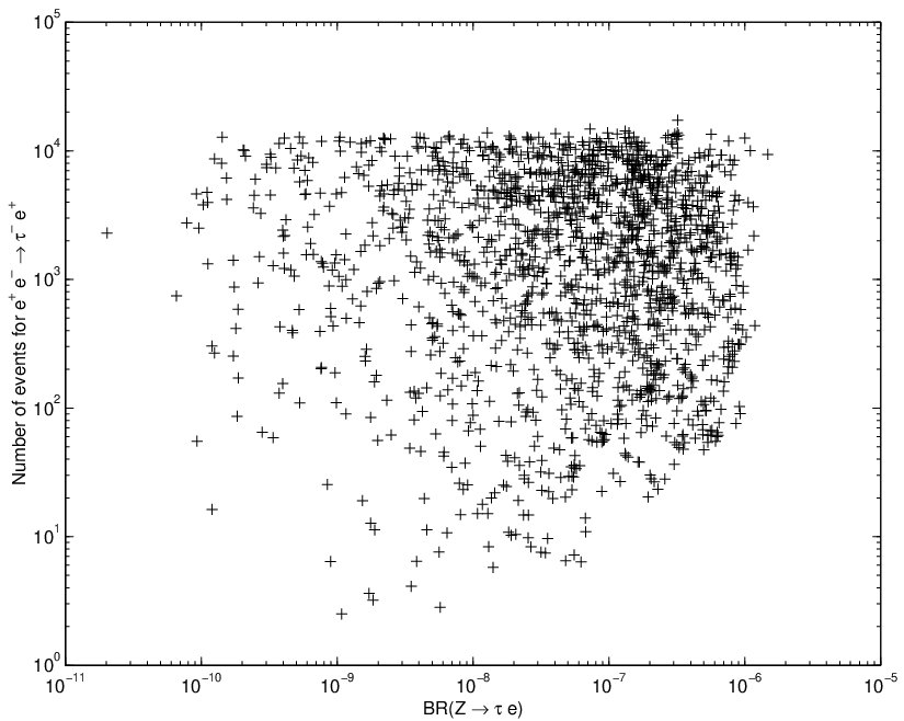
Refer to caption
Figure 4.7: Number of expected events at the ILC for the reaction e+​e−→τ−​e+e^{+}\,e^{-}\,\rightarrow\,\tau^{-}\,e^{+}, with a center-of-mass energy of 1 TeV and a total luminosity of 1 ab-1.

e+​e−→τ−​e+e^{+}\,e^{-}\,\rightarrow\,\tau^{-}\,e^{+}, in terms of the branching ratio BR(Z→τ​e)(Z\,\rightarrow\,\tau\,e). To obtain the points shown in this graph, we demanded that the values of the effective couplings were such that all of the branching ratios for the decays of the τ\tau lepton into three light leptons and BR(Z→τ​μ)(Z\,\rightarrow\,\tau\,\mu) were smaller than the experimental upper bounds on those quantities shown in table 2.3. We observe that, even for fairly small values of the τ\tau flavour-violating decays (10−9−10−610^{-9}-10^{-6}), there is the possibility of a large number of events for the anomalous cross section.

By following the opposite procedure – requiring first that the branching ratios BR(Z→τ​e)(Z\,\rightarrow\,\tau\,e) and BR(Z→τ​μ)(Z\,\rightarrow\,\tau\,\mu) be according to the experimental values, and letting BR(τ→l​l​l)(\tau\,\rightarrow\,l\,l\,l) free, where ll is either an electron or a muon – we obtain the plot shown in figure 4.8. This time we analyse the process
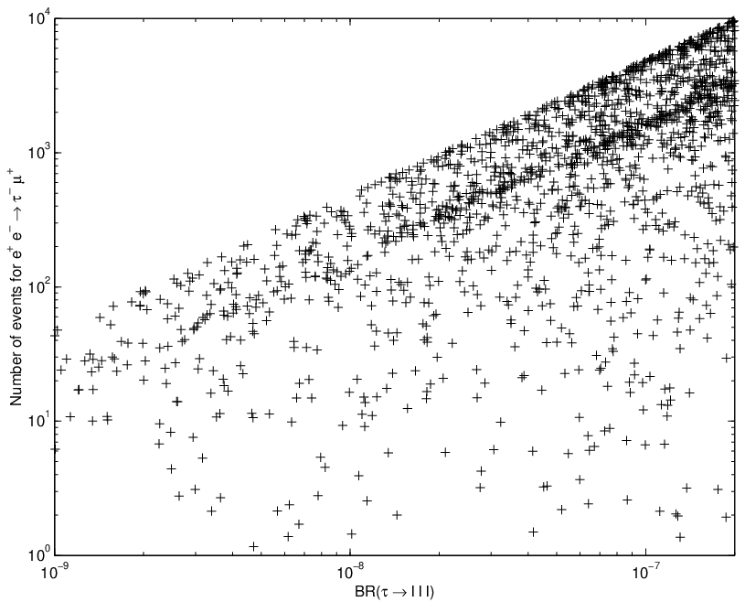
Refer to caption
Figure 4.8: Number of expected events at the ILC for the reaction e+​e−→τ−​μ+e^{+}\,e^{-}\,\rightarrow\,\tau^{-}\,\mu^{+}, with a center-of-mass energy of 1 TeV and a total luminosity of 1 ab-1.

e+​e−→τ−​μ+e^{+}\,e^{-}\,\rightarrow\,\tau^{-}\,\mu^{+}, but a similar plot is found for e+​e−→τ−​e+e^{+}\,e^{-}\,\rightarrow\,\tau^{-}\,e^{+}. The number of events rises sharply with increasing branching ratio of τ\tau into three leptons. It is possible to discern a thin “band” of events in the middle of points of figure 4.8, rising linearly with BR(τ→l​l​l)(\tau\,\rightarrow\,l\,l\,l). This “band” corresponds to events for which the four-fermion couplings are dominant over ZZ events. In that case, they dominate both BR(τ→l​l​l)(\tau\,\rightarrow\,l\,l\,l) and σ⁡(e+​e−→τ−​μ+)\sigma(e^{+}\,e^{-}\,\rightarrow\,\tau^{-}\,\mu^{+}), and the larger one is, the larger the other will be – which explains the linear growth of this subset of points in the plot of figure 4.8. This “isolated” contribution from the four-fermion terms is not visible in figure 4.7 since the branching ratios of the ZZ decays are independent of those same couplings. Finally and for completeness, in figure 4.9 we show the values of the asymmetry

Refer to caption
Figure 4.9: AF​B,RA_{FB,R} asymmetry for the process e+​e−→τ−​μ+e^{+}\,e^{-}\,\rightarrow\,\tau^{-}\,\mu^{+} versus B​R​(τ→l​l​l)BR(\tau\,\rightarrow\,l\,l\,l)

coefficient AF​B,RA_{FB,R} defined in (4.42), for the process e+​e−→τ−​μ+e^{+}\,e^{-}\,\rightarrow\,\tau^{-}\,\mu^{+}, versus the three-lepton decay of the τ\tau. A similar plot is obtained for the asymmetry AF​B,LA_{FB,L}. We observe a fairly uniform dependence on the branching ratio B​R​(τ→l​l​l)BR(\tau\,\rightarrow\,l\,l\,l), which is to say, on the values of the four-fermion couplings.

Finally, we also considered another possible process of LFV, namely γ​e−→μ−​Z\gamma\,e^{-}\,\rightarrow\,\mu^{-}\,Z. There are three Feynman diagrams contributing to this process, according the figure 4.10, one of which involving a quartic vertex which emerges from the effective operators of eqs. (4.1) and (4.2).

Refer to caption
Figure 4.10: Feynaman diagrams to e−​γ→μ−​Z.e^{-}\,\gamma\,\rightarrow\,\mu^{-}\,Z.

This process might occur at the ILC, if we consider the almost-collinear photons emitted by the colliding leptons, well described by the so-called equivalent photon approximation (EPA) [129]. An estimate of the cross section for this process, however, showed it to be much lower than the remaining ones we considered in this thesis. This is due to the EPA introducing an extra electromagnetic coupling constant into the cross section, and also to the fact that the final state of this process includes at least three particles (one of the beam particles “survives” the interaction) – thus there is, compared to the other processes which have only leptons in the final state, an additional phase space suppression. Notice, however, that an optional upgrade for the ILC is to have e​γe\,\gamma collisions, with center-of-mass energies and luminosities similar to those of the e+​e−e^{+}\,e^{-} mode, so this cross section might become important.

The flavour-violating channels are experimentally interesting, as they present a final state with an extremely clear signal, which can be easily identified. The argument is that the final state will always present two very energetic leptons of different flavour, more to the point, an electron and a muon. LFV can be seen in one of the three channels e+​e−→μ−​e+,e^{+}\,e^{-}\rightarrow\mu^{-}\,e^{+}, e+​e−→τ−​e+,e^{+}\,e^{-}\rightarrow\tau^{-}\,e^{+}, e+​e−→τ−​μ+,e^{+}\,e^{-}\rightarrow\tau^{-}\,\mu^{+}, and charge conjugate channels. The first channel is the best one, with the two leptons back to back and almost free of backgrounds. For the other production processes, we may “select” the decays of the tau that best suit our purposes: for the second we should take the tau decay τ−→μ−​ν¯μ​ντ,\tau^{-}\rightarrow\mu^{-}\bar{\nu}_{\mu}\nu_{\tau}, and for the third process, τ−→e−​ν¯e​ντ.\tau^{-}\rightarrow e^{-}\bar{\nu}_{e}\nu_{\tau}. The branching ratios for both of these tau decays are around 17%, so the loss of signal is affordable. The conclusion is that, for every lepton flavour-violating process, one can always end up with a final state with an electron and a muon. If the ILC detectors have superb detection performances for these particles, then the odds of observing violation of the leptonic number at the ILC, if those processes do exist, seem reasonable.

Clearly, our prediction that significant numbers of anomalous events may be produced at the ILC needs to be further investigated including the effects of a real detector. Notice also that due to beamstrahlung effects which reduce the effective beam energy, the total LFVevent rates might be reduced, specially in the case of the four-fermion cross sections, which increase with s.s. Also, one must take into account the many different backgrounds that could mask our signal. And the fact that, even in the best case scenario, only a few thousand events are produced with an integrated luminosity of 1​a​b−1,1\;ab^{-1}, could limit the signal-to-background ratio. We can show that with some very simple cuts most of the background can be eliminated. Because of the weaker experimental constraints on processes involving τ\tau leptons, the most promising LFV reactions at the linear collider are μ​e\mu\,e and μ​τ\mu\,\tau production. For illustrative purposes we will study the backgrounds to the LFV process e+​e−→τ+​e−→μ+​e−​νμ​ν¯τ.e^{+}\,e^{-}\rightarrow\tau^{+}\,e^{-}\rightarrow\mu^{+}\,e^{-}\,\nu_{\mu}\bar{\nu}_{\tau}. The main source of background to this process are e+​e−→μ+​e−​νμ​ν¯ee^{+}\,e^{-}\rightarrow\mu^{+}\,e^{-}\,\nu_{\mu}\bar{\nu}_{e} and e+​e−→τ+​τ−→μ+​e−​νμ​ν¯e​ντ​ν¯τ.e^{+}\,e^{-}\rightarrow\tau^{+}\,\tau^{-}\rightarrow\mu^{+}\,e^{-}\,\nu_{\mu}\bar{\nu}_{e}\,\nu_{\tau}\,\bar{\nu}_{\tau}. The cross section to the background process e+​e−→μ+​e−​νμ​ν¯ee^{+}\,e^{-}\rightarrow\mu^{+}\,e^{-}\,\nu_{\mu}\bar{\nu}_{e} was calculated using WPHACT [131] and confirmed using RACOONWW [133]. The cross section for the remaining background was evaluated using PYTHIA [134]. In e+​e−→τ+​e−→μ+​e−​νμ​ν¯τe^{+}\,e^{-}\rightarrow\tau^{+}\,e^{-}\rightarrow\mu^{+}\,e^{-}\,\nu_{\mu}\bar{\nu}_{\tau} the electron is produced in a two body final state. Therefore its energy is approximately half of the center-of-mass energy. Furthermore, if θe\theta_{e} is the angle between the electron and the beam, then the transverse momentum of the electron is pT=s/2sinθe.p_{T}=\sqrt{s}/2\,\sin\theta_{e}. This means that a cut in θe\theta_{e} implies a cut in pT.p_{T}. The main contribution to this cross section comes from the fourfermion interaction. There are no propagators involved and consequently the dependence in θe\theta_{e} (and in pTp_{T}) is very mild. This can be seen from the expression 4.53 in the Appendix 4.A. Making all coupling constants Vi​jV_{ij} and Si​jS_{ij} equal, it can be shown that a 10∘10^{\circ} cut will reduce the cross section by 2% while a 60∘60^{\circ} cut will reduce it only by 58%. In Table 4.1 we show the cross sections for the signal and for the backgrounds as a function of a cut in θe\theta_{e} and a corresponding cut in pT.p_{T}.

Cut in θe\theta_{e} (degrees) 10 20 30 40 50 60
e+​e−→τ+​e−→μ+​e−​νμ​ν¯τe^{+}\,e^{-}\rightarrow\tau^{+}\,e^{-}\rightarrow\mu^{+}\,e^{-}\,\nu_{\mu}\,\bar{\nu}_{\tau} 4.9 4.6 4.1 3.5 2.8 2.1
e+​e−→μ+​e−​νμ​ν¯ee^{+}\,e^{-}\rightarrow\mu^{+}\,e^{-}\,\nu_{\mu}\,\bar{\nu}_{e} 68.2 26.3 10.8 4.4 1.6 0.5
e+​e−→τ+​τ−→μ+​e−​νμ​ν¯e​ντ​ν¯τe^{+}\,e^{-}\rightarrow\tau^{+}\,\tau^{-}\rightarrow\mu^{+}\,e^{-}\,\nu_{\mu}\,\bar{\nu}_{e}\,\nu_{\tau}\,\bar{\nu}_{\tau} 1.3 0.8 0.3 0.2 0.06 0.01
Table 4.1: Cross section (in OPENf​b​a​r​n)fbarn) for the LFV signal and most relevant backgrounds to that process for several values of the angle cut between the outgoing electron and the beam axis.

For the signal we start with a cross section of 5​f​b​a​r​n5\;fbarn when no cuts are applied. Because of the mild dependence on θe\theta_{e}, a cut of 60 degrees will make the signal well above background. A further cut on the energy of the electron could be applied, say Ee>300​G​e​V.E_{e}>300\;GeV. This would not affect the signal but will reduce the background even further. All calculations were performed at tree level with initial state radiation and final state radiation turned off. Another possibility for background reduction would be to use the polarization of the beams, a method known to be very efficient. Notice, however, that this procedure might affect the extraction of four-fermion couplings from polarized beam experiments – if the signal is observed only for certain combinations of beam polarizations, it could happen that only certain couplings, or combinations thereof, can be measured.

Finally, some comments on the dependence of these results vis-a-vis expected improvements on the measurements of the LFV branching ratios of tab 2.3. Could it be that future experiments would tighten the constraints so much that there was no room available for discovery? Tau physics at BABAR and BELLE has provided the best limits so far on LFV involving the τ\tau lepton. The combined results from BABAR and BELLE on τ→l​γ.\tau\rightarrow l\gamma. are now reaching the level of 10−810^{-8} and will be close to just a few 10−810^{-8} by 2008 [135]. More important to us are the decays τ→l​l​l,\tau\rightarrow lll, due to the constraints imposed on the four fermion operators. The latest results on B​r​(τ→l​l​l)Br(\tau\rightarrow lll) from BABAR and BELLE are of the order of 10−7,10^{-7}, with less than 100​f​b−1100\;fb^{-1} of data analysed. A value of the order of a few 10−810^{-8} is expected when all data is taken into account [136]. Other planned experiments like MEG or SINDRUM2 (see [137]) will provide much more precise results for both μ→e​γ\mu\rightarrow e\gamma and μ​e\mu e conversion, respectively. However, those results will not constrain any further the four-fermion couplings. The current limit B​r​(μ→e​e​e)<10−12Br(\mu\rightarrow eee)<10^{-12} at 90%90\% CL [138] already excludes the possibility of finding LFV in the μ​e​e​e\mu eee coupling. This limit will be improved by the Sundrum experiment (see [137]). Another possibility is the GigaZ option for the ILC, which probably would be earlier than an energy upgrade to 1​T​e​V.1TeV. Again, the limits on the LFV branching ratios of the ZZ boson would be improved [139] but the bounds on the four-fermion couplings would not be affected. Lastly, LFV searches will also take place at the LHC. Preparatory studies on the LFV decay τ→μ​μ​μ\tau\rightarrow\mu\mu\mu are being conducted by CMS [140], ATLAS [31] and also by LHCb [141]. During the initial low luminosity runs (10−30​f​b−1/y​e​a​r)(10-30\;fb^{-1}/year) for 2008-2009, searches for this decay may be possible. So far the limits predicted are only slightly better than the known limits from the BB-factories. Therefore, in the foreseeable future, the constraints on the four fermion τ\tau couplings arising from the branching ratios of table I could go down one order of magnitude, to the order of 10−8.10^{-8}. Accordingly, and repeating the calculations that led to figs. 4.7 and 4.8, the maximum number of events expected at the ILC also goes down by one order of magnitude, to about 1000 events. Given the discussion on backgrounds above, we expect that detection of LFV at the ILC would still be possible, although harder.

Appendix 4.A Single top production via gamma-gamma collisions

In section 4.2.1 we argued that the couplings corresponding to the operators of eqs. ()– (4.3) were extremely limited in size by the existing experimental data for the branching ratios of the decays lh→ll​γl_{h}\,\rightarrow\,l_{l}\,\gamma. In fact, we even showed that the cross sections for the processes γ​γ→lh​ll\gamma\,\gamma\,\rightarrow\,l_{h}\,l_{l}, eq. (4.19), were directly proportional to those branching ratios, and their values at the ILC were predicted to be exceedingly small. It is easy to understand, though, that we has defined operators analogous to those of eqs. (4.3) for quarks instead of leptons. In particular, we considered flavour-changing operators involving the top quark, which would describe decays such as t→u​γt\,\rightarrow\,u\,\gamma or t→c​γt\,\rightarrow\,c\,\gamma - and these decay widths have not yet been measured. The total top quark width being also a lot larger than the tau’s or the muon’s, it seems possible that the cross section for single top production via flavour-violating photon-photon interactions may well present us with observable values.

The corresponding calculation (eq. 3.13) is altogether identical to the one we presented for the leptonic case. We find an expression for the width of the anomalous decay t→q​γt\,\rightarrow\,q\,\gamma nearly identical to that of eq. (4.14). Likewise, considering that the top quark’s charge is 2/32/3 and the quarks have three colour degrees of freedom, we may rewrite the analog of eq. (4.19) as

d​σ​(γ​γ→t​q¯)d​t=−16​π​α​Fγ​γ3​mt3​s​(mt2−t)2​t​(mt2−u)2​u​Γ​(t→q​γ),\frac{d\sigma(\gamma\,\gamma\,\rightarrow\,t\,\bar{q})}{dt}\;\;=\;\;-\,\frac{16\pi\alpha\,F_{\gamma\gamma}}{3\,{m_{t}}^{3}\,s\,{({m_{t}}^{2}-t)}^{2}\,t\,{({m_{t}}^{2}-u)}^{2}\,u}\;\Gamma(t\,\rightarrow\,q\,\gamma)\;\;\;, (4.46)

with Fγ​γF_{\gamma\gamma} given by an expression identical to eq. (4.20), with the substitution mh↔mtm_{h}\,\leftrightarrow\,m_{t}. With a top total width of about 1.42 GeV and for s\sqrt{s} equal to 1 TeV, this expression can be integrated in tt (with a pTp_{T} cut of 10 GeV on the final state particles, to prevent any collinear singularities) and the total cross section estimated to be of the order

σ⁡(γ​γ→t​q¯)∼\displaystyle\sigma(\gamma\,\gamma\,\rightarrow\,t\,\bar{q})\;\sim    90×BR​(t→q​γ)​pb.\displaystyle\;\;\;90\,\times\,\mbox{BR}(t\,\rightarrow\,q\,\gamma)\;\;\mbox{pb}\;\;\;. (4.47)

We see a considerable difference vis-a-vis the predicted leptonic cross sections, from eqs. (4.21) - this one is much larger. To pass from the photon-photon cross section to an electron-positron process, we apply the standard procedure: use the equivalent photon approximation [129] to provide us with the probability of an electron/positron with energy EE radiating photons with a fraction xx of E and integrate eq. (4.46) over xx. For recent studies of photon-photon collisions at the ILC, see for instance [142]. The numerical result we found for the single top production cross section is

σ⁡(e+​e−→e+​e−​t​q¯)=  1.08×BR​(t→q​γ)​pb.\sigma(e^{+}\,e^{-}\,\rightarrow\,e^{+}\,e^{-}\,t\,\bar{q})\;\;=\;\;1.08\,\times\,\mbox{BR}(t\,\rightarrow\,q\,\gamma)\;\;\mbox{pb}\;\;\;. (4.48)

For an integrated luminosity of about 1 ab-1, this gives us about one event observed at the ILC for branching ratios of t→q​γt\,\rightarrow\,q\,\gamma near the maximum of its theoretical predictions 33 3 Obtained in several models, such the two-Higgs doublet model or R-parity violationg SUSY theories [74]., ∼ 10−6\sim\,10^{-6}. Clearly, this result means that this process should not be observed at the ILC, even in the best case scenario. However, in the event of non-observation, eq. (4.48) could be useful to impose an indirect limit on the branching ratio BR​(t→q​γ)\mbox{BR}(t\,\rightarrow\,q\,\gamma). Several authors have studied single top production in e+​e−e^{+}\,e^{-} collisions [126, 143]. For gamma-gamma reactions, single top production at the ILC in the framework of the effective operator formalism may has been studied in [147], and for specific models, such as SUSY and technicolor, in ref. [142].

Appendix 4.B Total cross section expressions

We write the amplitude for the four-fermion cross sections in two parts. One for the ss channel and the other one for the tt channel. In doing so we are generalizing the four-fermion Lagrangian which for a gauge theory has equal couplings for both ss and tt channels. For the ss channel the amplitude reads

Ti​js=1Λ4​[Vi​js​(v¯e​γα​γi​ue)​(u¯lh​γα​γj​vll)+Si​js​(v¯e​γi​ue)​(u¯lh​γj​vll)]T_{ij}^{s}\,=\,\frac{1}{\Lambda^{4}}\left[V_{ij}^{s}\,(\bar{v}_{e}\gamma_{\alpha}\gamma_{i}u_{e})(\bar{u}_{l_{h}}\gamma^{\alpha}\gamma_{j}v_{l_{l}})\,+\,\,S_{ij}^{s}\,(\bar{v}_{e}\gamma_{i}u_{e})(\bar{u}_{l_{h}}\gamma_{j}v_{l_{l}})\right] (4.49)

while for the t channel we have

Ti​jt=−1Λ4​[Vi​jt​(u¯lh​γα​γi​ue)​(v¯e​γα​γj​ve)+Si​jt​(u¯lh​γi​ue)​(v¯e​γj​ve)]T_{ij}^{t}\,=\,-\,\frac{1}{\Lambda^{4}}\left[V_{ij}^{t}\,(\bar{u}_{l_{h}}\gamma_{\alpha}\gamma_{i}u_{e})(\bar{v}_{e}\gamma^{\alpha}\gamma_{j}v_{e})\,+\,\,S_{ij}^{t}\,(\bar{u}_{l_{h}}\gamma_{i}u_{e})(\bar{v}_{e}\gamma_{j}v_{e})\right] (4.50)

with i,j=L,Ri,j=L,R. With these definitions we can write

|T⁡(eL−​eL+→lhL−​llL+)|2=\displaystyle|T(e_{L}^{-}e_{L}^{+}\rightarrow{l_{h}}_{L}^{-}{l_{l}}_{L}^{+})|^{2}\,= 1Λ4​(4​u2​|VL​Ls+VL​Lt|2)\displaystyle\,\frac{1}{\Lambda^{4}}(4u^{2}|V_{LL}^{s}+V_{LL}^{t}|^{2})
|T⁡(eR−​eR+→lhR−​llR+)|2=\displaystyle|T(e_{R}^{-}e_{R}^{+}\rightarrow{l_{h}}_{R}^{-}{l_{l}}_{R}^{+})|^{2}\,= 1Λ4​(4​u2​|VR​Rs+VR​Rt|2)\displaystyle\,\frac{1}{\Lambda^{4}}(4u^{2}|V_{RR}^{s}+V_{RR}^{t}|^{2})
|T⁡(eL−​eL+→lhR−​llR+)|2=\displaystyle|T(e_{L}^{-}e_{L}^{+}\rightarrow{l_{h}}_{R}^{-}{l_{l}}_{R}^{+})|^{2}\,= 1Λ4​t2​|SR​Lt|2\displaystyle\,\frac{1}{\Lambda^{4}}\,t^{2}\,|S_{RL}^{t}|^{2}
|T⁡(eR−​eR+→lhL−​llL+)|2=\displaystyle|T(e_{R}^{-}e_{R}^{+}\rightarrow{l_{h}}_{L}^{-}{l_{l}}_{L}^{+})|^{2}\,= 1Λ4​t2​|SL​Rt|2\displaystyle\,\frac{1}{\Lambda^{4}}t^{2}\,|S_{LR}^{t}|^{2}
|T⁡(eL−​eR+→lhL−​llR+)|2=\displaystyle|T(e_{L}^{-}e_{R}^{+}\rightarrow{l_{h}}_{L}^{-}{l_{l}}_{R}^{+})|^{2}\,= 1Λ4​s2​|SL​Rs|2\displaystyle\,\frac{1}{\Lambda^{4}}\,s^{2}\,|S_{LR}^{s}|^{2}
|T⁡(eR−​eL+→lhR−​llL+)|2=\displaystyle|T(e_{R}^{-}e_{L}^{+}\rightarrow{l_{h}}_{R}^{-}{l_{l}}_{L}^{+})|^{2}\,= 1Λ4​s2​|SR​Ls|2\displaystyle\,\frac{1}{\Lambda^{4}}\,s^{2}\,|S_{RL}^{s}|^{2} (4.51)

and to obtain the expressions when only the tt or ss channels are present, you just have to set the ss couplings or the tt couplings, respectively, equal to zero. uu, tt and ss are the Mandelstam variables defined in the usual way.

The cross sections for polarized electron and positron beams with no detection of the polarization of the final state particles were given in eq. (4.31). The International Linear Collider will have a definite degree of polarization that will depend on the final design of the machine. For longitudinal polarized beams the cross section can be written as

d​σPe−​Pe+d​t=\displaystyle\frac{d\sigma_{P_{e^{-}}P_{e^{+}}}}{dt}\,= 14[(1+Pe−)(1+Pe+)d​σR​Rd​t+(1−Pe−)(1−Pe+)d​σL​Ld​t+\displaystyle\,\frac{1}{4}\biggl[(1+P_{e^{-}})(1+P_{e^{+}})\frac{d\sigma_{RR}}{dt}\,+\,(1-P_{e^{-}})(1-P_{e^{+}})\frac{d\sigma_{LL}}{dt}+
(1+Pe−)(1−Pe+)d​σR​Ld​t+(1−Pe−)(1+Pe+)d​σL​Rd​t]\displaystyle(1+P_{e^{-}})(1-P_{e^{+}})\frac{d\sigma_{RL}}{dt}\,+\,(1-P_{e^{-}})(1+P_{e^{+}})\frac{d\sigma_{LR}}{dt}\biggr] (4.52)

where σR​L\sigma_{RL} corresponds to a cross section where the electron beam is completely right-handed polarized (Pe−=+1P_{e^{-}}=+1) and the positron beam is completely left-handed polarized (Pe+=−1P_{e^{+}}=-1). This reduces to the usual averaging over spins in the case of totally unpolarized beams. For the general expression for polarized beams, as well as a study on all the advantages of using those beams, see [128].

In the main text we presented expressions for the differential cross sections. For completeness we now present the formulae for the total cross sections. For the four-fermion case, the expressions have a very simple dependence on the pTp_{T} cut one might wish to apply, so we exhibit it. The quantity x=1−4​pT2/sx=\sqrt{1-4p_{T}^{2}/s}, with pTp_{T} being the value of the minimum transverse momentum for the heaviest lepton, gives us an immediate way of obtaining these cross sections with a cut on the pTp_{T} of the final particles. The total cross section is obviously the sum over all polarized ones, which gives us

σ=s​x​(3+x2)768​π​Λ4​(4​|VL​Ls+VL​Lt|2+|SR​Lt|2+4​|VR​Rs+VR​Rt|2+|SL​Rt|2)+s​x64​π​(|SL​Rs|2+|SR​Ls|2).\sigma\,=\,\frac{s\,x\,(3+x^{2})}{768\pi\Lambda^{4}}\left(4\,|V_{LL}^{s}+V_{LL}^{t}|^{2}+|S_{RL}^{t}|^{2}+4\,|V_{RR}^{s}+V_{RR}^{t}|^{2}+|S_{LR}^{t}|^{2}\right)+\,\frac{s\,x}{64\pi}\left(|S_{LR}^{s}|^{2}+|S_{RL}^{s}|^{2}\right)\,. (4.53)

As explained in the main text, the cross sections for processes (1,2)(1,2) are obtained from eq. (4.53) by setting all of the “s” couplings equal to the “t” ones, and, for process (3)(3), by setting the “t” couplings to zero.

For the remaining cross section expressions we imposed no pTp_{T} cut on any of the final particles. The total cross section for the ZZ couplings is given by, for processes (1,2)(1,2),

σZ(1,2)​(e−​e+→lh​ll)=\displaystyle\sigma_{Z}^{(1,2)}(e^{-}e^{+}\rightarrow l_{h}l_{l})\;= v2192​π​Λ4​Mz2​s2​(Mz2−s)2​(Mz2+s)[F3(gA)|ηl​h|2\displaystyle\;\;\frac{v^{2}}{192\,\pi\,\Lambda^{4}\,M_{z}^{2}\,s^{2}\,(M_{z}^{2}-s)^{2}\,(M_{z}^{2}+s)}\left[F_{3}(g_{A})|\eta_{lh}|^{2}\right.\vskip 8.5359pt
+F3(−gA)|ηh​l|2+F4(gA)|θL|2+F4(−gA)|θR|2],\displaystyle\;\left.+F_{3}(-g_{A})|\eta_{hl}|^{2}+F_{4}(g_{A})|\theta_{L}|^{2}+F_{4}(-g_{A})|\theta_{R}|^{2}\right]\,\,, (4.54)

with

F3​(gA)\displaystyle F_{3}(g_{A}) =6​s​Mz2​(Mz4−s2)​log⁡(Mz2+sMz2)\displaystyle=6\,s\,M_{z}^{2}\,(M_{z}^{4}-s^{2})\log\left(\frac{M_{z}^{2}+s}{M_{z}^{2}}\right)
×[(gA−gV)2​Mz4−2​(gA2+gA​gV+gV2)​s​Mz2−(gA2+gV2)​s2]−s2​Mz2​(Mz2+s)\displaystyle\times\left[(g_{A}-g_{V})^{2}M_{z}^{4}-2(g_{A}^{2}+g_{A}g_{V}+g_{V}^{2})sM_{z}^{2}-(g_{A}^{2}+g_{V}^{2})s^{2}\right]-s^{2}\,M_{z}^{2}\,(M_{z}^{2}+s)
×[6​(gA−gV)2​Mz4−3​(7​gA2−2​gA​gV+7​gV2)​s​Mz2+2​(7​gA2+3​gA​gV+7​gV2)​s2]\displaystyle\times\left[6(g_{A}-g_{V})^{2}M_{z}^{4}-3(7g_{A}^{2}-2g_{A}g_{V}+7g_{V}^{2})sM_{z}^{2}+2(7g_{A}^{2}+3g_{A}g_{V}+7g_{V}^{2})s^{2}\right]
F4​(gA)=\displaystyle F_{4}(g_{A})\;=   48​v2​(Mz4−s2)​(Mz2+s)​Mz4​log⁡(Mz2Mz2+s)​(gA−gV)2\displaystyle\;\;48v^{2}(M_{z}^{4}-s^{2})(M_{z}^{2}+s)M_{z}^{4}\log\left(\frac{M_{z}^{2}}{M_{z}^{2}+s}\right)(g_{A}-g_{V})^{2}
+8v2s[3(gA−gV)2Mz6(2Mz2+s)−(5gA2−18gAgV+5gV2)s2Mz4\displaystyle+8v^{2}s\left[3(g_{A}-g_{V})^{2}M_{z}^{6}(2M_{z}^{2}+s)-(5g_{A}^{2}-18g_{A}g_{V}+5g_{V}^{2})s^{2}M_{z}^{4}\right.
−5(gA2+gV2)s3Mz2+3(gA2+gV2)s4],\displaystyle\left.-5(g_{A}^{2}+g_{V}^{2})s^{3}M_{z}^{2}+3(g_{A}^{2}+g_{V}^{2})s^{4}\right],

with interference terms

σi​n​t(1,2)=\displaystyle\sigma_{int}^{(1,2)}\;= −v248​Λ4​π​(s−Mz2)​s2{\displaystyle\;\;-\,\frac{v^{2}}{48\,\Lambda^{4}\,\pi\,(s-M_{z}^{2})\,s^{2}}\biggr\{\vskip 8.5359pt
s[(gA−gV){(12Mz4+6sMz2−14s2)Re(θLVL​L∗)−s2Re(θRSR​L∗)}\displaystyle s\biggr[\left(g_{A}-g_{V}\right)\left\{(12M_{z}^{4}+6sM_{z}^{2}-14s^{2})\mbox{Re}\left(\theta_{L}V_{LL}^{*}\right)-s^{2}\mbox{Re}\left(\theta_{R}S_{RL}^{*}\right)\right\}\vskip 8.5359pt
−(gA+gV){(12Mz4+6sMz2−14s2)Re(θRVR​R∗)−s2Re(θLSL​R∗)}]\displaystyle\,\,-\left(g_{A}+g_{V}\right)\left\{(12M_{z}^{4}+6sM_{z}^{2}-14s^{2})\mbox{Re}\left(\theta_{R}V_{RR}^{*}\right)-s^{2}\mbox{Re}\left(\theta_{L}S_{LR}^{*}\right)\right\}\biggl]\vskip 8.5359pt
+ 3(Mz2−s)[(gA−gV){(4Mz4+8sMz2−4s2)Re(θLVL​L∗)−s2Re(θRSR​L∗)}\displaystyle+\,3\,(M_{z}^{2}-s)\biggr[\left(g_{A}-g_{V}\right)\left\{(4M_{z}^{4}+8sM_{z}^{2}-4s^{2})\mbox{Re}\left(\theta_{L}V_{LL}^{*}\right)-s^{2}\mbox{Re}\left(\theta_{R}S_{RL}^{*}\right)\right\}\vskip 8.5359pt
−(gA+gV){(4Mz4+8sMz2−4s2)Re(θRVR​R∗)−s2Re(θLSL​R∗)}]\displaystyle\,\,-\left(g_{A}+g_{V}\right)\left\{(4M_{z}^{4}+8sM_{z}^{2}-4s^{2})\mbox{Re}\left(\theta_{R}V_{RR}^{*}\right)-s^{2}\mbox{Re}\left(\theta_{L}S_{LR}^{*}\right)\right\}\biggl]\vskip 8.5359pt
log(Mz2Mz2+s)}.\displaystyle\log\left(\frac{M_{z}^{2}}{M_{z}^{2}+s}\right)\biggl\}\;\;\;. (4.55)

Finally, for process (3)(3), we have

σZ(3)=(gV2+gA2)​v2​s192​π​Λ4​(Mz2−s)2​[8​(|θL|2+|θR|2)​v2+(|ηh​l|2+|ηl​h|2)​s],\sigma_{Z}^{(3)}\;=\;\frac{\left(g_{V}^{2}+g_{A}^{2}\right)v^{2}s}{192\,\pi\,\Lambda^{4}\,(M_{z}^{2}-s)^{2}}\left[8\left(|\theta_{L}|^{2}+|\theta_{R}|^{2}\right)v^{2}+\left(|\eta_{hl}|^{2}+|\eta_{lh}|^{2}\right)s\right]\,\,, (4.56)

and

σi​n​t(3)=\displaystyle\sigma_{int}^{(3)}\;= s​v224​π​(s−Mz2)​Λ4​[(gV+gA)​Re​(θR​VR​R∗)+(gV−gA)​Re​(θL​VL​L∗)].\displaystyle\;\frac{sv^{2}}{24\pi(s-M_{z}^{2})\,\Lambda^{4}}\left[\left(g_{V}+g_{A}\right)\mbox{Re}\left(\theta_{R}V_{RR}^{*}\right)+\left(g_{V}-g_{A}\right)\,\mbox{Re}\left(\theta_{L}V_{LL}^{*}\right)\right]\;\;\;. (4.57)

Appendix 4.C Numerical values for decay widths and cross sections

We present here numerical values for the several decay widths and cross sections given in the text. We have set, in the following expressions, Λ\Lambda to 1​T​e​V,1\;TeV, the dependence in Λ\Lambda being trivially recovered if we wish a different value for it.

BR4​f​(μ→l​l​l)\displaystyle\mbox{BR}_{4f}(\mu\rightarrow lll) = 2.3×10⁻⁴​(|SL​R|2+|SR​L|2+4​(|VL​L|2+|VR​R|2))\displaystyle=\;2.3\times 10^{-4}(|S_{LR}|^{2}+|S_{RL}|^{2}+4(|V_{LL}|^{2}+|V_{RR}|^{2}))\vskip 11.38092pt
BR4​f​(τ→l​l​l)\displaystyle\mbox{BR}_{4f}(\tau\rightarrow lll) = 4.0×10⁻⁵​(|SL​R|2+|SR​L|2+4​(|VL​L|2+|VR​R|2))\displaystyle=\;4.0\times 10^{-5}(|S_{LR}|^{2}+|S_{RL}|^{2}+4(|V_{LL}|^{2}+|V_{RR}|^{2}))\vskip 11.38092pt
BRZ​(μ→l​l​l)\displaystyle\mbox{BR}_{Z}(\mu\rightarrow lll) = 8.2×10⁻⁴​(|θL|2+|θR|2)+2.5×10⁻⁷​Re​(ηl​h​θL∗+ηh​l​θR)\displaystyle=\;8.2\times 10^{-4}\left(|\theta_{L}|^{2}+|\theta_{R}|^{2}\right)+2.5\times 10^{-7}\mbox{Re}\left(\eta_{lh}\theta_{L}^{*}+\eta_{hl}\theta_{R}\right)\vskip 11.38092pt
BRZ​(τ→l​l​l)\displaystyle\mbox{BR}_{Z}(\tau\rightarrow lll) = 1.4×10⁻⁴​(|θL|2+|θR|2)+7.3×10⁻⁷​Re​(ηl​h​θL∗+ηh​l​θR)\displaystyle=\;1.4\times 10^{-4}\left(|\theta_{L}|^{2}+|\theta_{R}|^{2}\right)+7.3\times 10^{-7}\mbox{Re}\left(\eta_{lh}\theta_{L}^{*}+\eta_{hl}\theta_{R}\right)\vskip 11.38092pt
BRi​n​t​(μ→l​l​l)\displaystyle\mbox{BR}_{int}(\mu\rightarrow lll) =−1.4×10⁻³Re(θLVL​L∗)+1.1×10⁻³Re(θRVR​R∗)\displaystyle=\;-1.4\times 10^{-3}\mbox{Re}\left(\theta_{L}V_{LL}^{*}\right)+1.1\times 10^{-3}\mbox{Re}\left(\theta_{R}V_{RR}^{*}\right)\vskip 11.38092pt
+ 1.7×10⁻⁷Re(ηl​hVR​R∗)−2.1×10⁻⁷Re(ηh​lVL​L)\displaystyle\;+\,1.7\times 10^{-7}Re\left(\eta_{lh}V_{RR}^{*}\right)-2.1\times 10^{-7}\mbox{Re}\left(\eta_{hl}V_{LL}\right)\vskip 11.38092pt
BRi​n​t​(τ→l​l​l)\displaystyle\mbox{BR}_{int}(\tau\rightarrow lll) =−2.4×10⁻⁴Re(θLVL​L∗)+1.9×10⁻⁴Re(θRVR​R∗)\displaystyle=\;-2.4\times 10^{-4}Re\left(\theta_{L}V_{LL}^{*}\right)+1.9\times 10^{-4}\mbox{Re}\left(\theta_{R}V_{RR}^{*}\right)\vskip 11.38092pt
+ 4.8×10⁻⁷Re(ηl​hVR​R∗)−6.0×10⁻⁷Re(ηh​lVL​L).\displaystyle\;+\,4.8\times 10^{-7}Re\left(\eta_{lh}V_{RR}^{*}\right)-6.0\times 10^{-7}\mbox{Re}\left(\eta_{hl}V_{LL}\right)\;\;\;. (4.58)
BR​(Z→l​l)\displaystyle\mbox{BR}(Z\rightarrow ll) = 2.3×10⁻⁵​(|ηh​l|2+|ηl​h|2)+6.7×10⁻⁴​(|θL|2+|θR|2)\displaystyle=\;2.3\times 10^{-5}(|\eta_{hl}|^{2}+|\eta_{lh}|^{2})+6.7\times 10^{-4}(|\theta_{L}|^{2}+|\theta_{R}|^{2})
BR​(Z→μ​l)\displaystyle\mbox{BR}(Z\rightarrow\mu l) =B​r​(Z→l​l)−2.0×10⁻⁷​Re​(θL​ηh​l+θR​ηl​h∗)\displaystyle=\;Br(Z\rightarrow ll)-2.0\times 10^{-7}\mbox{Re}\left(\theta_{L}\eta_{hl}+\theta_{R}\eta_{lh}^{*}\right)
BR​(Z→τ​l)\displaystyle\mbox{BR}(Z\rightarrow\tau l) =B​r​(Z→l​l)−2.4×10⁻⁶​Re​(θL​ηh​l+θR​ηl​h∗).\displaystyle=\;Br(Z\rightarrow ll)-2.4\times 10^{-6}\mbox{Re}\left(\theta_{L}\eta_{hl}+\theta_{R}\eta_{lh}^{*}\right)\;\;\;. (4.59)

For the cross sections, taking s=1\sqrt{s}=1 TeV and imposing a cut of 10 GeV on the pTp_{T} of the particles in the final state, we have (in picobarn):

σ4​f(1,2)​(e−​e+→l​l)\displaystyle\sigma_{4f}^{(1,2)}(e^{-}e^{+}\rightarrow ll) = 2.58​(|SL​R|2+|SR​L|2)+10.33​(|VL​L|2+|VR​R|2)\displaystyle=\;2.58\left(|S_{LR}|^{2}+|S_{RL}|^{2}\right)+10.33\left(|V_{LL}|^{2}+|V_{RR}|^{2}\right)
σ4​f(3)​(e−​e+→l​l)\displaystyle\sigma_{4f}^{(3)}(e^{-}e^{+}\rightarrow ll) = 1.94​(|SL​R|2+|SR​L|2)+2.58​(|VL​L|2+|VR​R|2)\displaystyle=\;1.94\left(|S_{LR}|^{2}+|S_{RL}|^{2}\right)+2.58\left(|V_{LL}|^{2}+|V_{RR}|^{2}\right)
σZ(1,2)​(e−​e+→l​l)\displaystyle\sigma_{Z}^{(1,2)}(e^{-}e^{+}\rightarrow ll) = 1.0×10⁻²|ηl​h|2+9.7×10⁻³|ηh​l|2+5.7×10⁻²(θL|2+|θR|2)\displaystyle=\;1.0\times 10^{-2}|\eta_{lh}|^{2}+9.7\times 10^{-3}|\eta_{hl}|^{2}+5.7\times 10^{-2}\left(\theta_{L}|^{2}+|\theta_{R}|^{2}\right)
σZ(3)​(e−​e+→l​l)\displaystyle\sigma_{Z}^{(3)}(e^{-}e^{+}\rightarrow ll) = 1.6×10⁻⁴​(|θL|2+|θR|2)+6.7×10⁻⁴​(|ηh​l|2+|ηl​h|2)\displaystyle=\;1.6\times 10^{-4}\left(|\theta_{L}|^{2}+|\theta_{R}|^{2}\right)+6.7\times 10^{-4}\left(|\eta_{hl}|^{2}+|\eta_{lh}|^{2}\right)
σi​n​t(1,2)​(e−​e+→l​l)\displaystyle\sigma_{int}^{(1,2)}(e^{-}e^{+}\rightarrow ll) = 0.70​Re​(θL​VL​L∗)+0.19​Re​(θL​SR​L∗)−0.56​Re​(θR​VR​R∗)−0.24​Re​(θR​SL​R∗)\displaystyle=\;0.70\,\mbox{Re}\left(\theta_{L}V_{LL}^{*}\right)+0.19\,\mbox{Re}\left(\theta_{L}S_{RL}^{*}\right)-0.56\,\mbox{Re}\left(\theta_{R}V_{RR}^{*}\right)-0.24\,\mbox{Re}\left(\theta_{R}S_{LR}^{*}\right)
σi​n​t(3)​(e−​e+→l​l)\displaystyle\sigma_{int}^{(3)}(e^{-}e^{+}\rightarrow ll) =−2.6×10⁻²Re(θRVR​R∗)+3.2×10⁻²Re(θLVL​L∗).\displaystyle=\;-2.6\times 10^{-2}\,\mbox{Re}\left(\theta_{R}V_{RR}^{*}\right)+3.2\times 10^{-2}\,\mbox{Re}\left(\theta_{L}V_{LL}^{*}\right)\;\;\;. (4.60)

References

  • [1] P. M. Ferreira, R. B. Guedes, and R. Santos, Phys. Rev. D75, 055015 (2007), hep-ph/0611222
  • [2] P. M. Ferreira, R. B. Guedes, and R. Santos, Phys. Rev. D77, 114008 (2008), 0802.2075
  • [3] R. A. Coimbra et al., (in preparation.)
  • [4] E. Malkawi and T. Tait, Phys. Rev. D54, 5758 (1996), hep-ph/9511337
  • [5] T. Han, K. Whisnant, B. L. Young, and X. Zhang, Phys. Lett. B385, 311 (1996), hep-ph/9606231
  • [6] T. Han, K. Whisnant, B. L. Young, and X. Zhang, Phys. Rev. D55, 7241 (1997), hep-ph/9603247
  • [7] K. Whisnant, J.-M. Yang, B.-L. Young, and X. Zhang, Phys. Rev. D56, 467 (1997), hep-ph/9702305
  • [8] M. Hosch, K. Whisnant, and B. L. Young, Phys. Rev. D56, 5725 (1997), hep-ph/9703450
  • [9] T. Han, M. Hosch, K. Whisnant, B.-L. Young, and X. Zhang, Phys. Rev. D58, 073008 (1998), hep-ph/9806486
  • [10] T. Tait and C. P. Yuan, Phys. Rev. D63, 014018 (2001), hep-ph/0007298
  • [11] D. O. Carlson, E. Malkawi, and C. P. Yuan, Phys. Lett. B337, 145 (1994), hep-ph/9405277
  • [12] T. G. Rizzo, Phys. Rev. D53, 6218 (1996), hep-ph/9506351
  • [13] T. Tait and C. P. Yuan, Phys. Rev. D55, 7300 (1997), hep-ph/9611244
  • [14] D. Espriu and J. Manzano, Phys. Rev. D65, 073005 (2002), hep-ph/0107112
  • [15] K.-i. Hikasa, K. Whisnant, J. M. Yang, and B.-L. Young, Phys. Rev. D58, 114003 (1998), hep-ph/9806401
  • [16] P. M. Ferreira, O. Oliveira, and R. Santos, Phys. Rev. D73, 034011 (2006), hep-ph/0510087
  • [17] P. M. Ferreira and R. Santos, Phys. Rev. D73, 054025 (2006), hep-ph/0601078
  • [18] P. M. Ferreira and R. Santos, Phys. Rev. D74, 014006 (2006), hep-ph/0604144
  • [19] W. Buchmuller and D. Wyler, Nucl. Phys. B268, 621 (1986)
  • [20] J. N. Bahcall, R. D. Jr., P. Parker, A. Smirnov, and R. Ulrich, Solar Neutrinos - The First Thirty Years (Addison-Wesley, 1995)
  • [21] R. N. Mohapatra and P. B. Pal, Massive Neutrinos in Physics and Astrophysics (World Scientific, 2005)
  • [22] G. L. Fogli, E. Lisi, A. Marrone, and A. Palazzo, Prog. Part. Nucl. Phys. 57, 742 (2006), hep-ph/0506083
  • [23] SNO, B. Aharmim et al., Phys. Rev. C75, 045502 (2007), nucl-ex/0610020
  • [24] SNO, B. Aharmim et al., Phys. Rev. C72, 055502 (2005), nucl-ex/0502021
  • [25] SNO, Q. R. Ahmad et al., Phys. Rev. Lett. 89, 011301 (2002), nucl-ex/0204008
  • [26] A. Barroso and J. P. Silva, Phys. Rev. D50, 4581 (1994), hep-ph/9404246
  • [27] Particle Data Group, W. M. Yao et al., J. Phys. G33, 1 (2006)
  • [28] D. Delepine and F. Vissani, Phys. Lett. B522, 95 (2001), hep-ph/0106287
  • [29] J. I. Illana and T. Riemann, Phys. Rev. D63, 053004 (2001), hep-ph/0010193
  • [30] A. Flores-Tlalpa, J. M. Hernandez, G. Tavares-Velasco, and J. J. Toscano, Phys. Rev. D65, 073010 (2002), hep-ph/0112065
  • [31] M. A. Perez, G. Tavares-Velasco, and J. J. Toscano, Int. J. Mod. Phys. A19, 159 (2004), hep-ph/0305227
  • [32] M. Frank and H. Hamidian, Phys. Rev. D54, 6790 (1996), hep-ph/9603222
  • [33] A. Ghosal, Y. Koide, and H. Fusaoka, Phys. Rev. D64, 053012 (2001), hep-ph/0104104
  • [34] E. O. Iltan and I. Turan, Phys. Rev. D65, 013001 (2002), hep-ph/0106068
  • [35] C.-x. Yue, H. Li, Y.-m. Zhang, and Y. Jia, Phys. Lett. B536, 67 (2002), hep-ph/0204153
  • [36] J. Cao, Z. Xiong, and J. M. Yang, Eur. Phys. J. C32, 245 (2004), hep-ph/0307126
  • [37] C.-x. Yue, W. Wang, and F. Zhang, J. Phys. G30, 1065 (2004), hep-ph/0406235
  • [38] E. O. Iltan, Eur. Phys. J. C46, 487 (2006), hep-ph/0507213
  • [39] F. Deppisch, H. Pas, A. Redelbach, R. Ruckl, and Y. Shimizu, Phys. Rev. D69, 054014 (2004), hep-ph/0310053
  • [40] Y.-B. Sun et al., JHEP 09, 043 (2004), hep-ph/0409240
  • [41] M. Cannoni, S. Kolb, and O. Panella, Phys. Rev. D68, 096002 (2003), hep-ph/0306170
  • [42] M. Cannoni, C. Carimalo, W. Da Silva, and O. Panella, Phys. Rev. D72, 115004 (2005), hep-ph/0508256
  • [43] A. Ibarra, E. Masso, and J. Redondo, Nucl. Phys. B715, 523 (2005), hep-ph/0410386
  • [44] A. V. Manohar, (1996), hep-ph/9606222
  • [45] B.-L. Young, Chin. J. Phys. 34, 418 (1997)
  • [46] J. Wudka, AIP Conf. Proc. 531, 81 (2000), hep-ph/0002180
  • [47] I. Z. Rothstein, (2003), hep-ph/0308266
  • [48] C. P. Burgess, Annu. Rev. Nucl. Part. Sci. 57, 329 (2007)
  • [49] Z. Han, (2008), 0807.0490
  • [50] T. L. Cheng, Search for Anomalous Single Top Quark Production via FCNC with the ATLAS Detector at the LHC, PhD thesis, Royal Holloway, University of London, 2007
  • [51] C.-N. Yang and R. L. Mills, Phys. Rev. 96, 191 (1954)
  • [52] E. S. Abers and B. W. Lee, Phys. Rept. 9, 1 (1973)
  • [53] P. W. Higgs, Phys. Rev. Lett. 13, 508 (1964)
  • [54] P. W. Higgs, Phys. Rev. 145, 1156 (1966)
  • [55] S. Weinberg, Phys. Rev. Lett. 19, 1264 (1967)
  • [56] A. Salam, Weak and electromagnetic interactions, in Elementary Particle Theory, edited by N. Svartholm, pp. 367–377, Almquist and Wiksell, Stockholm, 1968
  • [57] H. Fritzsch, M. Gell-Mann, and H. Leutwyler, Phys. Lett. B47, 365 (1973)
  • [58] G. ’t Hooft, Nucl. Phys. B33, 173 (1971)
  • [59] E. A. Paschos, Electroweak theory , Cambridge, UK: Univ. Pr. (2007) 245 p
  • [60] D0, S. Abachi et al., Phys. Rev. Lett. 74, 2632 (1995), hep-ex/9503003
  • [61] CDF, F. Abe et al., Phys. Rev. Lett. 74, 2626 (1995), hep-ex/9503002
  • [62] CDF, (2007), hep-ex/0703034
  • [63] M. Beneke et al., (2000), hep-ph/0003033
  • [64] N. Kidonakis and R. Vogt, Phys. Rev. D68, 114014 (2003), hep-ph/0308222
  • [65] R. Bonciani, S. Catani, M. L. Mangano, and P. Nason, Nucl. Phys. B529, 424 (1998), hep-ph/9801375
  • [66] C. I. Ciobanu, Acta Phys. Polon. B Proceedings Supplement B1 - n 2, 245 (2008)
  • [67] D0, V. M. Abazov et al., Phys. Rev. Lett. 98, 181802 (2007), hep-ex/0612052
  • [68] Z. Sullivan, Phys. Rev. D70, 114012 (2004), hep-ph/0408049
  • [69] J. Campbell and F. Tramontano, Nucl. Phys. B726, 109 (2005), hep-ph/0506289
  • [70] S. L. Glashow, J. Iliopoulos, and L. Maiani, Phys. Rev. D2, 1285 (1970)
  • [71] S. L. Glashow and S. Weinberg, Phys. Rev. D15, 1958 (1977)
  • [72] E. A. Paschos, Phys. Rev. D15, 1966 (1977)
  • [73] J. A. Aguilar-Saavedra, Acta Phys. Polon. B35, 2695 (2004), hep-ph/0409342
  • [74] M. E. Luke and M. J. Savage, Phys. Lett. B307, 387 (1993), hep-ph/9303249
  • [75] D. Atwood, L. Reina, and A. Soni, Phys. Rev. D55, 3156 (1997), hep-ph/9609279
  • [76] J. M. Yang, B.-L. Young, and X. Zhang, Phys. Rev. D58, 055001 (1998), hep-ph/9705341
  • [77] J. Guasch and J. Sola, Nucl. Phys. B562, 3 (1999), hep-ph/9906268
  • [78] D. Delepine and S. Khalil, Phys. Lett. B599, 62 (2004), hep-ph/0406264
  • [79] J. J. Liu, C. S. Li, L. L. Yang, and L. G. Jin, Phys. Lett. B599, 92 (2004), hep-ph/0406155
  • [80] G. Eilam, M. Frank, and I. Turan, Phys. Rev. D74, 035012 (2006), hep-ph/0601253
  • [81] J. J. Cao et al., Phys. Rev. D75, 075021 (2007), hep-ph/0702264
  • [82] A. Arhrib and W.-S. Hou, JHEP 07, 009 (2006), hep-ph/0602035
  • [83] A. Arhrib, K. Cheung, C.-W. Chiang, and T.-C. Yuan, Phys. Rev. D73, 075015 (2006), hep-ph/0602175
  • [84] J. Guasch, W. Hollik, S. Penaranda, and J. Sola, Nucl. Phys. Proc. Suppl. 157, 152 (2006), hep-ph/0601218
  • [85] D. Lopez-Val, J. Guasch, and J. Sola, JHEP 12, 054 (2007), 0710.0587
  • [86] J. A. Aguilar-Saavedra, Phys. Rev. D67, 035003 (2003), hep-ph/0210112
  • [87] F. del Aguila, J. A. Aguilar-Saavedra, and R. Miquel, Phys. Rev. Lett. 82, 1628 (1999), hep-ph/9808400
  • [88] T. P. Cheng and M. Sher, Phys. Rev. D35, 3484 (1987)
  • [89] S. Bejar, J. Guasch, and J. Sola, Nucl. Phys. B600, 21 (2001), hep-ph/0011091
  • [90] C. S. Li, R. J. Oakes, and J. M. Yang, Phys. Rev. D49, 293 (1994)
  • [91] G. M. de Divitiis, R. Petronzio, and L. Silvestrini, Nucl. Phys. B504, 45 (1997), hep-ph/9704244
  • [92] J. L. Lopez, D. V. Nanopoulos, and R. Rangarajan, Phys. Rev. D56, 3100 (1997), hep-ph/9702350
  • [93] G. Eilam, A. Gemintern, T. Han, J. M. Yang, and X. Zhang, Phys. Lett. B510, 227 (2001), hep-ph/0102037
  • [94] F. del Aguila et al., (2008), 0801.1800
  • [95] P. J. Fox, Z. Ligeti, M. Papucci, G. Perez, and M. D. Schwartz, (2007), 0704.1482
  • [96] F. Larios, R. Martinez, and M. A. Perez, Phys. Rev. D72, 057504 (2005), hep-ph/0412222
  • [97] R. D. Peccei, S. Peris, and X. Zhang, Nucl. Phys. B349, 305 (1991)
  • [98] T. Han, R. D. Peccei, and X. Zhang, Nucl. Phys. B454, 527 (1995), hep-ph/9506461
  • [99] R. Martinez, M. A. Perez, and J. J. Toscano, Phys. Lett. B340, 91 (1994)
  • [100] ALEPH, A. Heister et al., Phys. Lett. B543, 173 (2002), hep-ex/0206070
  • [101] DELPHI, J. Abdallah et al., Phys. Lett. B590, 21 (2004), hep-ex/0404014
  • [102] OPAL, G. Abbiendi et al., Phys. Lett. B521, 181 (2001), hep-ex/0110009
  • [103] L3, P. Achard et al., Phys. Lett. B549, 290 (2002), hep-ex/0210041
  • [104] ZEUS, S. Chekanov et al., Phys. Lett. B559, 153 (2003), hep-ex/0302010
  • [105] CDF, . T. Aaltonen, (2008), 0805.2109
  • [106] CDF, F. Abe et al., Phys. Rev. Lett. 80, 2525 (1998)
  • [107] A. A. Ashimova and S. R. Slabospitsky, (2006), hep-ph/0604119
  • [108] H1, A. Aktas et al., Eur. Phys. J. C33, 9 (2004), hep-ex/0310032
  • [109] D0, V. M. Abazov et al., Phys. Rev. Lett. 99, 191802 (2007), hep-ex/0702005
  • [110] ATLAS, J. Carvalho et al., Eur. Phys. J. C52, 999 (2007), 0712.1127
  • [111] CMS, G. L. Bayatian et al., J. Phys. G34, 995 (2007)
  • [112] M. Battaglia et al., (2006), hep-ex/0603010
  • [113] L. H. Ryder, Quantum Field Theory (Cambridge University Press, Cambridge, 1996)
  • [114] F. del Aguila, J. A. Aguilar-Saavedra, and L. Ametller, Phys. Lett. B462, 310 (1999), hep-ph/9906462
  • [115] F. del Aguila and J. A. Aguilar-Saavedra, Nucl. Phys. B576, 56 (2000), hep-ph/9909222
  • [116] A. Denner and T. Sack, Nucl. Phys. B358, 46 (1991)
  • [117] G. Eilam, R. R. Mendel, R. Migneron, and A. Soni, Phys. Rev. Lett. 66, 3105 (1991)
  • [118] A. Czarnecki and K. Melnikov, Nucl. Phys. B544, 520 (1999), hep-ph/9806244
  • [119] K. G. Chetyrkin, R. Harlander, T. Seidensticker, and M. Steinhauser, Phys. Rev. D60, 114015 (1999), hep-ph/9906273
  • [120] S. M. Oliveira, L. Brucher, R. Santos, and A. Barroso, Phys. Rev. D64, 017301 (2001), hep-ph/0011324
  • [121] M. Won, Combined Effects of Strong and Electroweak Effective FCNC Operators in Top Production at the LHC, Master’s thesis, Faculdade de Ciências e Tecnologia da Universidade de Coimbra, Coimbra, 2008
  • [122] J. Pumplin et al., JHEP 07, 012 (2002), hep-ph/0201195
  • [123] S. R. Slabospitsky and L. Sonnenschein, Comput. Phys. Commun. 148, 87 (2002), hep-ph/0201292
  • [124] N. Castro, (unpuplished.)
  • [125] N. Kidonakis and A. Belyaev, JHEP 12, 004 (2003), hep-ph/0310299
  • [126] S. Bar-Shalom and J. Wudka, Phys. Rev. D60, 094016 (1999), hep-ph/9905407
  • [127] B. Grzadkowski, Z. Hioki, K. Ohkuma, and J. Wudka, Nucl. Phys. B689, 108 (2004), hep-ph/0310159
  • [128] G. A. Moortgat-Pick et al., Phys. Rept. 460, 131 (2008), hep-ph/0507011
  • [129] S. J. Brodsky, T. Kinoshita, and H. Terazawa, Phys. Rev. D4, 1532 (1971)
  • [130] L. E. Gordon, Phys. Rev. D50, 6753 (1994)
  • [131] E. Accomando, A. Ballestrero, and E. Maina, Comput. Phys. Commun. 150, 166 (2003), hep-ph/0204052
  • [132] E. Accomando and A. Ballestrero, Comput. Phys. Commun. 99, 270 (1997), hep-ph/9607317
  • [133] A. Denner, S. Dittmaier, M. Roth, and D. Wackeroth, Comput. Phys. Commun. 153, 462 (2003), hep-ph/0209330
  • [134] T. Sjostrand et al., Comput. Phys. Commun. 135, 238 (2001), hep-ph/0010017
  • [135] S. Banerjee, Nucl. Phys. Proc. Suppl. 169, 199 (2007), hep-ex/0702017
  • [136] F. Salvatore, (private communication)
  • [137] D. Nicolo, Lepton Violation Searches with μ\mu-Beams: Status and Perspectives, in XXXX Rencontres de Moriond
  • [138] G. Wilson, Physics; theory and experimental analysis: Alternative Theories, in DESY/ECFA LC98 workshops
  • [139] SINDRUM, U. Bellgardt et al., Nucl. Phys. B299, 1 (1988)
  • [140] T. Mori, Nucl. Phys. Proc. Suppl. 169, 166 (2007)
  • [141] M. Shapkin, Nucl. Phys. Proc. Suppl. 169, 363 (2007)
  • [142] J.-j. Cao, G.-l. Liu, and J. M. Yang, Eur. Phys. J. C41, 381 (2005), hep-ph/0311166
  • [143] T. Han and J. L. Hewett, Phys. Rev. D60, 074015 (1999), hep-ph/9811237
  • [144] Y. P. Gouz and S. R. Slabospitsky, Phys. Lett. B457, 177 (1999), hep-ph/9811330
  • [145] K.-i. Hikasa, Phys. Lett. B149, 221 (1984)
  • [146] J.-j. Cao, Z.-h. Xiong, and J. M. Yang, Nucl. Phys. B651, 87 (2003), hep-ph/0208035
  • [147] Y. Jiang et al., Phys. Rev. D57, 4343 (1998), hep-ph/9801206
  • [148] Z.-H. Yu, H. Pietschmann, W.-G. Ma, L. Han, and J. Yi, Eur. Phys. J. C16, 541 (2000), hep-ph/9903471
  • [149] K. J. Abraham, K. Whisnant, and B. L. Young, Phys. Lett. B419, 381 (1998), hep-ph/9707476.