Applied High Energy QCD
Abstract
These lectures stress the theoretical elements that underlie a wide range of phenomenological studies of high-energy QCD, which include both soft and hard processes. After a brief introduction to the basics of QCD, various aspects of QCD-based phenomenology are covered: colour transparency, hadronization of colour charges, Regge phenomenology, parton model, Bjorken scaling and its violation, DGLAP evolution equation, BFKL formalism, GLR-MQ evolution equation and saturation. In the last part of the lecture, we employ the light-cone dipole formalism to describe deep inelastic lepton scattering, Drell-Yan processes, direct photon production, diffraction, quark and gluon shadowing in nuclei, the Cronin effect and nuclear broadening.
1 The theory of strong interaction
Strong interactions are described by a quantum field theory known as quantum chromodynamics (QCD). In many ways QCD is a unique theory. Quantum electrodynamics (QED), and its expansion to the electroweak Standard Model of particle physics, is also a quantum field theory. QED is a renormalizable theory but it loses all its credibility as we approach the energy scale, the so-called Landau pole position, where the strength of the coupling constant (the strength of the interaction) becomes infinite11 1 The dependence of coupling constants on the energy scale is one of the basic ideas behind the renormalization group which will be discussed in Section 1.3.. On the other hand, if the cutoff goes to infinity, QED becomes trivial. QED is not the only theory with a Landau pole problem; every theory which is not asymptotically free suffers from this problem. QCD is the only known theory which is free from such problems. QCD needs only a few parameters to be defined completely: one universal coupling strength and one mass for each kind of quark.
Despite more than half a century of attempts, our knowledge about many aspects of QCD is still rudimentary. This is mainly due to the fact that QCD evolves from a few-body theory of free quarks and gluons at short distances to an extremely complicated infinite-body theory of objects like hadrons and nuclei, giving rise to a variety of complex physical systems and their interactions. The aim of this manuscript is to bring together various aspects of high-energy nuclear physics as tools for studying QCD itself.
1.1 QCD Lagrangian and it symmetries
The Lagrangian of QCD is given by
| (1) |
where is the quark field which is defined in the fundamental representation of the colour and flavor group, and the conjugate Dirac field is defined as . The gluon field matrix is defined in the fundamental representation where denotes the number of colour, being the generators of the gauge group which satisfies where are the structure constants of . We define as the strong coupling constant. The field strength is given by
| (2) |
The non-Abelian nature of QCD is manifested by the quadratic term in the gauge field strength, which gives rise to gluon-gluon interactions shown in Fig. 1. The crucial difference between QCD and QED is the presence of this quadratic term which makes the QCD field equations non-linear. These nonlinearities give rise to a non-trivial dynamics and various rich structures which are unique properties of the strong interaction. The colour and flavour indices of the quark field are suppressed. is the current quark mass which is not directly observable if QCD confines quarks. The current quark mass is colour independent and can be brought diagonal in flavour space. There are six flavours of quarks, each of which has a different mass. The three light quarks are called up (u), down (d) and strange (s), while the three heavy quarks are called charm (c), bottom (b) and top (t). The following values for the light current quark masses are found in the Particle Data tables [1],
| (3) |

Notice that the quark masses are renormalization-scheme dependent. The above values are obtained in a subtraction scheme at a renormalization scale . In addition to flavour, quarks carry another quantum number known as colour. Each quark comes in three colours which, based on a convention, are called red, green and blue.
The Lagrangian Eq. (1) has a large classical symmetry: we have the local gauge symmetry by construction,
In QED, there is only one electric charge, and the gauge transformation involves a single phase factor . The QCD Lagrangian Eq. (1) has also a global flavour symmetry which does not affect the gluon fields,
| (4) |
where denotes the generators of the flavour group and denotes the number of flavors. The above symmetry is referred to as vector flavor symmetry . When the generator is the unit matrix, we have symmetry associated with conservation of baryon number. There is another global symmetry which is exact at , namely chiral symmetry. This symmetry is very similar to vector flavor symmetry, apart from an extra factor of in the generator of the transformation.
| (5) |
Notice that due to the factor the quark field and its conjugate partner are transformed by the same matrix in contrast to vector transformation Eq. (4). This transformation Eq. (5) is called the axial-vector transformation and can be combined with the vector transformation to define a bigger symmetry at chiral which is then called chiral symmetry . One may alternatively define right- and left-handed quark fields by following transformation
| (6) |
The right- and left-handed massless fermions are eigenvalues of the helicity or chirality (with eigenvalue ) and are not mixed together. The chiral symmetry can be equivalently written as .
Not all the above-mentioned symmetries survive quantization. Particles with opposite helicity are related by a parity transformation, therefore in a chirally symmetric world, the hadrons should come in parity doublets. However, in real life we do not observe such degeneracy. Therefore one can conclude that chiral symmetry is not realized in the ground state and chiral symmetry is spontaneously broken. A theory where the vacuum has less symmetry than the Lagrangian is called a theory with spontaneous symmetry breaking. The Goldstone theorem [6] tell us that the spontaneous breaking of a continuous global symmetry implies the existence of associated massless spinless particles. This indeed was confirmed due to the existence of the light pseudoscalar mesons in nature (pions, kaons and etas) which may be assigned as pseudo-Goldstone bosons [2]. Moreover, the existence of a quark condensate implies that the symmetry is spontaneously broken down to . Therefore one may conceive QCD quark condensate as an order parameter for chiral symmetry breaking. The concept of spontaneous broken chiral symmetry is the cornerstone in the understanding of the low-energy hadronic spectrum.

The symmetry implies that all hadrons should come with opposite parity partners. However, this is not the case, therefore this symmetry must be broken somehow. If the spontaneous symmetry breaking mechanism works here, then one should observe a Goldstone boson associated with , namely an pseudoscalar meson having roughly the same mass as the pion. Surprisingly there is no such Goldstone boson. This problem is sometime called puzzle. It turned out that the symmetry is explicitly broken by quantum effects. This effect is known as the axial anomaly [3]. The axial charge corresponding to the axial current is not conserved because of the contribution of the triangle graph in Fig. 2. The four-divergence of the axial current is given by
| (7) |
where is the dual field strength tensor. The last term (gluonic part) is a full divergence, and one may expect that this term not to have any physical effect if the QCD vacuum were trivial. It was shown by ’t Hoof that due to instanton effects, the symmetry is not manifested in nature [3].
Finally, at , the QCD Lagrangian is invariant under a scale transformation which is called dilatational symmetry:
| (8) |
This symmetry is again broken at the quantum level due to the trace anomaly [4].
1.2 QCD versus QED
Let us remember the main differences between QCD and QED. QCD is an extended version of QED which now, instead of one charge, has three different kinds of charge called colour. Similar to the photon in QED, here massless spin-one particles, the gluons, respond to the presence of colour charge. The colour charged quarks emit and absorb gluons in the same way as electrically charged leptons do. However, radiation of a photon does not change the charge of the electron, while a gluon can change the quark colour. The response of gluons to colour charge, as measured by the QCD coupling constant, is much more drastic than the response of photons to electric charge. Gluons, unlike photons, interact directly with each other, although the colour charges, like electric charge in QED, are conserved in all physical processes. Therefore gluons must be able to carry unbalanced colour charges in contrast to their counterpart the photon in QED.

In the following sections we shall also recapitulate the most important features of QCD which are not accessible perturbatively. These non-perturbative features are unique for QCD and should be traced back to the main differences between QCD and QED.
1.3 Asymptotic Freedom
Having introduced the gauge fixing term and an associated ghost term by means of the Faddeev-Popov procedure [5, 6], one can carry out perturbation theory in terms of coupling. Similar to QED, a dimensionless physical quantities can be expressed by a perturbation series in powers of the coupling parameter ( is the notation for ). Owing to the renormalization process, a renormalization scale enters the algebra [7] in order to remove the ultraviolet divergence. Therefore, one can write the dimensionless quantities in terms of other available dimensionless parameters and the renormalized coupling . However, the physical quantity cannot depend on the arbitrary . This means that should be renormalization scale invariant
| (9) |
This equation explicitly shows that any dependence of on must be cancelled by an appropriate -dependence of . It is also natural to identify the renormalization scale with the physical energy scale of the process, i.e. . The running coupling is described by the renormalization group equation [7],
| (10) |
Whenever the coupling is small, the function can be computed perturbatively,
| (11) |
with
| (12) |
Therefore one can readily calculate the effective running coupling at one-loop level ignoring the term,
| (13) |
where is a scale parameter of QCD and depends on the subtraction scheme and the number of active flavours. The present world average for at the mass is which leads to
| (14) |
where the symbol stands for minimal subtraction scheme [7] and the superscript indicates the number of active flavours. This value is taken from an analysis of various high energy processes [8, 9], see also Fig. 3. The most striking feature of the running coupling is that it decreases logarithmically with for when . This originates from the self-interaction of gluons which leads to anti-screening, in contrast to QED where the sign of is negative. Therefore perturbation theory works very well for large . This phenomenon is called asymptotic freedom [10]. However, if is near , perturbation theory does not work anymore and non-perturbative phenomena enter the stage. One of the biggest challenges of QCD is to connect these two domains. Admittedly, there is yet no unambiguous method to connect small and large distances in QCD.
1.4 Chiral symmetry breaking
In the first section, we introduced the symmetries of the QCD Lagrangian. In the limit of massless quarks, QCD possesses chiral symmetry which means that left- and right-handed quarks are not mixed,
| (15) |
As we already discussed, owing to the presence of the quark condensate , chiral symmetry is spontaneously broken and left- and right-handed quarks and antiquarks can transform into each other:
| (16) |
Dynamical chiral symmetry breaking is one of the important non-perturbative features of QCD which is responsible for the generation of quark masses22 2 There is another very different way to generate mass from vacuum, the so-called Casimir effect [11], which originates from the response of the vacuum in the presence of non-perturbative boundary conditions. The existence of boundary conditions in quantum field theory is not always free of problems (see, for example, Ref. [12]).. In order to show that this phenomenon is purely non-perturbative, we employ the QCD gap equation [13],
| (17) |
where and are the current-quark bare mass and the coupling constant, respectively. is the dressed-gluon propagator and is the dressed-quark-gluon vertex. The general solution of the gap equation is a dressed-quark propagator of the form
| (18) |
The functions and contain the effects of vector and scalar quark-dressing induced by the quark interaction with the gluon field. The function denotes the quark mass. One may now use the gap equation to work out the fermion self-energy perturbatively [14]. One obtains,
| (19) |
It is observed that at all orders of the loop expansion, terms are proportional to the current-quark mass and consequently vanish as . The quark mass is defined as a pole of the dressed-quark propagator; therefore no mass is generated at a current-quark mass equal to zero, i.e., the dynamical chiral symmetry breaking is impossible in perturbation theory and there is no mixing between left- and right-handed quarks at the perturbative level. Notice that, apart from the trivial solution at , a non-trivial solution can indeed be found at the chiral point, albeit accessible non-perturbatively. The renormalization effect is not included in Eq. (17), but it does not change the above argument [14]. The quark condensate33 3 Note that, at finite density and temperature, the formation of a quark cooper pair condensate is also possible, leading to colour symmetry breaking, the so-called colour superconductivity phenomenon(BCS) [15] and diquark Bose-Einstein condensation(BEC) [16]. in QCD is given by the trace of the full quark propagator Eq. (18),
| (20) |
Notice that since is a gauge invariant object, one may take any gauge to obtain the dressed quark propagator which has a general form as equation (18). It is obvious that when , the quark condensate does not take place, simply because of the identity . It has been shown in many non-perturbative approaches that the emergence of a dynamical quark mass leads to the non-vanishing of quark condensate and vice versa, see, for example, Refs. [17, 18].
1.5 Confinement
Another important non-perturbative feature of QCD is colour confinement [10]. Loosely speaking, confinement is defined as the absence of any free coloured objects in nature. But it is possible that there exists a composite coloured particle which can form colourless bound states with another coloured particle like quarks. Colour confinement is still not properly understood, and a clear and indisputable mechanism responsible for this effect remains yet to be discovered. The basic property of confinement can be explored by looking at heavy propagation at a large distance in a time interval . The behaviour of such a system can be described by the Wilson loop,
| (21) |
where denotes the generator of . One can show that at large interval of time ,
| (22) |
where is the static potential between the heavy quarks. At large distances this potential grows linearly:
| (23) |
Therefore the Wilson loop at large and behaves as , which is the so-called area low and indicates confinement.
Confinement originates non-perturbatively, since it is associated with a linear potential with a string tension
| (24) |
which is obviously non-perturbative in the coupling. Note that the string picture of quark confinement is not free of flaws, since string breaking will occur once the potential energy approaches the quark pair creation threshold.
It is well-known that for confinement it is sufficient that no coloured Schwinger function possesses a spectral representation. This is equivalent to say that all coloured Schwinger functions violate reflection positivity [13]. Another way of realization of QCD confinement is due to Gribov theory in which colour confinement is determined by the existence of very light (almost massless) quarks [19]. There are in fact many different ways that the confinement can be realized, such as monopole condensation, infrared enhancement of the ghost propagator, etc. For a review of this subject see Ref. [20].
One may wonder if there is a non-trivial solution for the gap equation which gives rise to a pole of the quark propagator, this might contradict QCD confinement since the quark is coloured. Indeed this is one of the subtle point in every QCD model and cannot be easily resolved. In principle, there will be a long-range force between massive quarks to confine them and also a short range spin-spin interaction between massive dressed quarks. The former will modify the low momentum part of the propagator to remove the quark from being on-shell. Actually, this describes a phenomenologically motivated picture of a constituent quark model based on the dynamical symmetry breaking. Having said that, it is very hard to incorporate the dynamical symmetry breaking and the confinement into a QCD model. In fact, many models constructed to describe the low-energy properties of hadrons [18, 21] are assumed to be only dominated by the quark flavor dynamics and dynamical symmetry breaking and are indeed reliable only at intermediate scales, between confinement scale few hundred MeV up to a scale about 1 GeV.
2 Evidences for coloured quarks
Historically, the idea of colour degree of freedom emerged as a viable solution to the problem of how to construct the wave function for the doubly charged baryons [22]. The wave function of in space, spin and flavour is symmetric and violates the Pauli exclusion principle since is fermion with spin . This problem was resolved by introducing a new degree of freedom, the colour degree of freedom, and requiring that the wave function to be antisymmetric in the colour degree of freedom.

Although coloured states are not detected in experiments, and only colour singlet states exist in nature, there is much experimental evidence in favour of a colour degree of freedom. One of the direct experimental test for a colour degree of freedom comes from annihilation into hadrons. In the annihilation process, first a pair of quarks is produced which then fragment into hadrons. The cross-section for producing a free pair is the same as for producing a pair except for the quark charge and colour number which should be replaced with the muon charge, see Fig. 4. Therefore in order to extract information about the QCD content of annihilation, in particular, the colour degree of freedom, it is convenient to express the total cross-section of annihilation in units of the cross-section of production,
| (25) |

The cross-section to produce any number of hadrons is proportional to that to produce a pair. This is because a highly virtual photons decays to quarks in a time scale (where is the center of mass energy), while a hadron with mass needs a formation time . Therefore, there is not enough time for confinement to affect the annihilation cross-section and one can assume that the produced pair fragments into hadrons with unit probability,
| (26) |
Therefore one finds
| (27) |
where the factor is the number of colour and denotes the quark charge. The summation in the above equation is over all flavours that are kinematically allowed. Depending on energy, various flavour degrees of freedom contribute,
| (28) |
up to about GeV only u, d and s contribute, while at higher energies charm and b quarks start contributing as well. If one assumes that , then Eq. (28) predicts and , respectively. If we ignore nonperturbative effects close to threshold, such as the formation of bound states, we expect to present a series of steps as a function of . In Fig. 5 we show various experimental data which shows remarkable agreement with more detailed perturbative QCD calculation based on the assumption that .
Another strong evidence of colour degree of freedom is the measurement of the neutral pion decay into photons . The pion decay rate is computed from the triangle diagram shown in Fig. 6. Because of the quark loops, the decay rate is proportional to . The experimental value of the pion decay rate can only be described by [24].
3 Colour transparency (CT)
So far we have treated colour as just a new quantum number, a new degree of freedom. Is there any evidence that this colour is responsible for the strong interactions?
If an interaction is controlled by colour, how can colourless hadrons interact? Apparently, only due to the spatial distribution of colour (carried by quarks and gluons) inside the hadrons, i.e., due to the existence of hadronic colour-dipole momentum.
This observation immediately leads to experimentally observable consequences. Since colourless dipoles of vanishing size cannot interact, the interaction cross-section of such a dipole (say, quark-antiquark) with other hadrons should vanish when the transverse dipole separation goes to zero [25],
| (29) |
This remarkable relation deserves commenting upon: (i) only transverse dipole separation matters, since at high energies longitudinal momentum transfer in exclusive reactions vanishes. For example, if the beam particle of mass and energy (in the target rest frame) is excited to mass , while the target remains intact, the longitudinal momentum transfer reads, ; (ii) the quadratic -dependence is dictated by dimension counting, no other dimension parameters can be used here (the QCD scale may enter only via the coupling ); (iii) an additional logarithmic dependence on may and does exist [25]; (iv) such a small- behaviour is common for QED and QCD; however, in the former case the total cross-section is predominantly elastic, while in the latter case is inelastic.

3.1 Quasielastic scattering off nuclei
The experimentally measured total hadronic cross-sections is a result of the interplay of different dipole sizes whose probabilities are controlled by the hadronic wave functions. In some cases the probability of small size configurations in a hadron can be enhanced leading to a reduced interaction cross-section of such a hadron. An example is elastic electron-proton scattering, , with high momentum transfer [26, 27], as illustrated in Fig, 7.
When the recoil proton has a reduced size44 4 Strictly speaking this is not a proton. This state can be projected either into a proton (as in the present case), or proton excitations., it should interact more weaker than a regular proton with other targets. Such a possibility exists, if the elastic scattering is embedded into a nucleus, i.e. in quasielastic reaction. The benchmark to compare with in this case is the expectations based on Glauber model calculations, where the recoil proton attenuates exponentially with the path length in the nucleus and with the normal proton-nucleon cross-section.
The observable usually measured in such experiments is nuclear transparency, defined as,
| (30) |
Basing on the above ideas of colour transparency one should expect a deviation rising with from the Glauber model predictions. Unfortunately no experiment performed so far has provided a clear evidence for such an effect. The results of the dedicated experiment NE18 at SLAC [28] are depicted in Fig. 8(right).

Apparently data show no preference either for Glauber, or CT based models [29]. Other measurements of reactions were not successful either, when searching for a CT signal. To fit the cross-section of this reaction by power -dependence, , a rise of with would be a signal of CT. However, the collection of data [30] depicted in Fig. 8(left) versus show no rise. Moreover, the value agrees with what one should expect from the Glauber model.
Analogously, experiment in quasielastic proton-proton scattering, , performed at BNL [31] did not provide any clear signal of CT. Although data deviates from the Glauber model predictions, at higher momentum transfers the agreement is restored.


Why did these experiments fail to observe a CT effect? It turns out that it is not enough to produce a small-sized configuration in a hard reaction. The produced hadron has to maintain this small size during propagation through the nucleus. It is clear that in a sufficiently long time interval the hadron will develop its wave function and restore the regular size. The time scale controlling this process is called formation time and for a recoil proton is given by,
| (31) |
Here is the energy of the recoil proton , and is the mass of the first proton excitation. In order to have for heavy nuclei , the proton energy should be much higher than . The highest energy of recoil protons in the NE18 experiment [28] was which is too low to keep the size of the produced hadron small within the nuclear range.
This is the principal problem of quasielastic scattering where the photon energy and virtuality are strongly correlated, . Thus the recoil proton energy is . Therefore one must go to extremely high virtualities, , just in order to increase . However, the cross-section becomes vanishingly small.
3.2 Diffractive electroproduction of vector mesons
Diffractive virtual photoproduction of vector mesons is free of this problem. The space-time development of this reaction is illustrated in Fig. 9

At very high energies, the fluctuation lifetime,
| (32) |
(which is also called coherence time), becomes very long. So one can treat the dipole propagating through the nucleus as ”frozen” by Lorentz time dilation at the initial size . Thus, one can keep the scale finite, while the photon (and vector meson) energy can be increased with no restriction. This is the main advantage of this process for the search for CT effects compared to quasielastic reactions. The first measurements proposed in [32] and performed by the E665 collaboration [34] confirmed the theoretical expectations [33] of CT effects depicted in Fig. 10(right). The high photon energy in this experiment led to and allowed us to greatly simplify theoretical calculations. It turns out that at the opposite limiting case of and high , the photon energy may be still high enough to keep the formation time scale Eq. (31) sufficiently long to observe CT effects. In this case a signal of CT would be a rising energy dependence of nuclear transparency. Corresponding measurements are under way at Jefferson Lab [30].


Similarly to diffraction, quasi-free hadron scattering off a nucleus can be performed at high energies, while the hadron size can be controlled by transverse momentum [35]. In the case of Reggeon exchange, the pion formfactor formfactor suppresses large-sized configurations in the hadronic wave function at rather small . Measurements were performed by the PROZA collaboration [36] with pions in quasi-free charge exchange scattering . The results are depicted in Fig. 10(left) in comparison with Glauber model expectations (dashed curve) and calculations including CT effects [35].
Notice that both models predict a peak at , because the cross-section of free scattering, , has a minimum at this momentum transfer, and the position of the minimum in quasi-free scattering is shifted by multiple interactions in the nucleus.
4 Bags, strings…
Gluonic condensate in vacuum pushes the energy density below the perturbative level, . If the colour field of the valence quarks suppresses vacuum fluctuations, then the energy density inside the hadron is higher than outside. Therefore the vacuum tries to squeeze the hadron. However, the chromo-electromagnetic energy inside a smaller volume rises leading to an equilibrium, as illustrated in Fig. 11(a).

Thus hadrons look like bubbles in the QCD vacuum, this is the key idea of the the MIT bag model [37].
What happens if a quark is knocked out with a high momentum? On account of the same properties of the QCD vacuum the chromo-electric flux is squeezed into a tube of a constant cross-section,
| (33) |
as illustrated in Fig. 11(b). Here is the colour charge at the ends of the tube; is the energy density stored in the tube per unit of length. This pattern of colour fields is quite different from that in QED, as illustrated in Fig. 12.
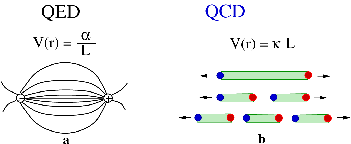
The potential between two electric charges falls with distance as , while in QCD it rises linearly. In fact, the rising with distance of a string potential explains the observed linearity of Regge trajectories (see below).
Usually the transverse size is not important, so the tube may be treated as a one-dimensional string, and is called string tension. It can be either calculated on the lattice, or related to the universal slope of Regge trajectories [38],
| (34) |
This energy is sufficient for the creation of a couple of constituent quarks via tunnelling from the vacuum. One can hardly stretch a string longer than 1fm, since it breaks into pieces, as illustrated in Fig. 12(b). The pairs produced from vacuum via the Schwinger mechanism completely screen the field of the end-point colour charges due to the linearity of the string potential [38]. The Schwinger phenomenon and existence of light quarks are the main reasons for not observing free quarks and gluons (colour screening).

5 Hadronization of colour charges
Thus a colour charge is always accompanied by an anti-charge neutralizing its colour. The colour field in between forms a tube/string which is a very unstable construction, pairs pop up via tunnelling from vacuum, as shown in Fig. 12(b), and the string is never much longer than . The probability of such a string breaking over time interval is given by,
| (35) |
where is the time-dependent length of the string, and the probability density for the creation of a pair per unit time per unit length is given by the Schwinger formula [38],
| (36) |
The string length is getting shorter after each break, thus delaying the next pair production. Therefore, hadron momenta rise in geometric progression, i.e. the rapidity distribution of produced hadrons is constant. Notice that such a plateau in rapidity has been predicted by models with multiperipheral dynamics and for gluon radiation in perturbative QCD [39]. This process is illustrated on a time-coordinate plot in the c.m. frame of the initial pair (e.g. annihilation), and in the target rest frame (e.g. in DIS) in Fig. 13 on the left and right correspondingly. Since both ends of the string are moving in the same direction and with the same velocity (the speed of light), the length of the string is independent of time. Its maximal possible value is . However, after each break of the string it becomes about twice as short, as illustrated in Fig. 13.
Notice that the leading quark loses energy at a constant rate, , though the whole hadronization process, until the creation of a hadron that includes this quark. It is interesting to notice that in perturbative QCD the leading quark loses energy for gluon radiation also at a constant rate, [40].
6 Regge phenomenology
The theory of Regge poles is a quite dormant topic. It does not
seem to be taught very much anymore. In addition there is often found an attitude that the subject is obsolete, because it is
identified so strongly with the pre-quark, pre-parton era of the
S-matrix, dispersion-relations approach to strong interactions.
This point of view is just plain wrong. The Chew, Frautschi, Regge, et. al., description of high energy
behaviour in terms of singularities in the complex angular momentum plane is completely general.
And the basic technique of Watson-Sommerfeld transform should
be a standard part of the training in theoretical particle physics.
—James Bjorken[41]

6.1 Poles in angular momentum plane
The energy dependence of the amplitude is governed by poles (or cuts) in the complex angular momentum plane [42],
| (37) |
where we sum over different Regge poles , and is a phenomenological residue function which is not given by the theory, but is fitted to data. It depends on , but not energy, and correlates with the choice of the parameter .
The phase factor depends on the Regge pole signature , where are spins (even or odd) of mesons lying on the trajectory.
| (38) |
The energy dependent factor is controlled by the Regge trajectory which is nearly straight, , as is demonstrated in on the Chew-Frautschi plot in Fig. 14. This is the miracle of Regge theory: the linear Regge trajectories bridge the low-energy physics of resonances () with high-energy scattering ().
High energies are dominated by Reggeons with highest trajectories , the Pomeranchuk pole (Pomeron),
| (39) |
and leading Reggeons,
| (40) |
The first important prediction of the Regge pole theory was shrinkage of the elastic slope with energy. The slope parameter controls the -dependence of the elastic cross-section, . According to (37) the slope parameter rises with energy as,
| (41) |
where is a phenomenological parameter.
The Pomeron parameters Eq. (39) were extracted from data on elastic scattering. The Pomeron intercept comes from data on total hadronic (mostly and ) cross-section fitted with the energy dependence (37), while the parameter is related to the elastic slope Eq. (41). Corresponding data are shown in Fig. 15.


6.2 Triple Regge phenomenology
The cross-section for the inclusive process, can be also expressed in terms of the Regge approach. Here we focus on the most interesting case of diffractive excitation, , via Pomeron exchange. To sum up all final-state excitations , one can apply the unitarity relation to the pomeron-hadron () amplitude as shown in Fig. 16. Provided that the effective mass of the excitation is large (but not too much), , one can describe the Pomeron-hadron elastic amplitude via Pomeron or secondary Reggeon exchanges in the -channel. Then one arrives at the triple-Regge graph, Fig. 16, which corresponds to the cross- section,
| (42) |
where is the Feynman variable for the recoil particle defined in the center of mass, .
Equation (42) contains new phenomenological functions, effective triple-Regge vertices, and . The diffractive cross-section can also be expressed in terms of the Pomeron-hadron total cross-section . Most interesting is the asymptotic () of this cross-section related to the triple-Pomeron coupling,
| (43) |

Here is the Pomeron-hadron vertex known from elastic scattering. Thus one can extract from data on single diffraction the Pomeron-hadron total cross-section, [45], which carries unique information about the properties of the Pomeron. The results shown in Fig. 17 demonstrate an amazingly small cross-section, less than .
This is at least an order of magnitude less than one could expect. Indeed, the Pomeron as a gluonic object should interact more strongly than a meson, i.e., the Pomeron-proton cross-section could be about twice as big as the pion-proton one. Such a weak interaction of the Pomeron is probably the strongest evidence for the location of the glue in hadrons within small spots [46].

6.3 Building the Pomeron
It has been a natural and simple assumption made in the early years of the Regge theory that the Pomeron is a Regge pole with a linear trajectory and the intercept . Nowadays, however, we have a multi-choice answer, and it is still debated whether the Pomeron is:
- •
a Regge pole (probably not, since varies with in DIS);
- •
- •
- •
something else?
Gluons seem to be the most suitable building material: already the Born graph provides . The higher order corrections are expected to pull the intercept above one. These corrections are dominated by ladder type graphs shown in Fig. 18.

A ladder is a shadow of gluon bremsstrahlung according to the unitarity relation, Fig. 39.
The leading-log approximation (LLA) corresponds to keeping those terms only, where each coupling has a big factor . For fixed coupling, the BFKL result is not a Regge pole, but a cut with an intercept
| (44) |
This result will be derived in Section 8, see Eq. (86). Unfortunately, the next-to-leading-log corrections (extra powers of ) to the intercept are of the same order [51],
| (45) |
and it may be even negative for most reasonable values of .
However, it does not look reasonable to describe a soft Pomeron, controlling soft hadronic interaction at high energies perturbatively. Similar latter graphs, but built of light hadrons, e.g. of pions and mesons as depicted in Fig. 19, well describe many features of soft hadronic collisions [52].

One can adjust the poorly known -pion coupling to reproduce the Pomeron intercept. However, its closeness to one, which is very natural in QCD, looks as an accidental coincidence in this model.
6.4 Duality
Reggeons correspond to the exchange of valence quarks. The descriptions of meson-meson scattering amplitude in terms of interacting pairs in the channel (Reggeons), or in the channel (resonances) are dual [42], as is illustrated in Fig. 20.

No channel resonances is possible in and elastic amplitudes. However, channel Reggeons are present. To comply with duality the Reggeons must cancel each other in the imaginary part of the amplitude. For this reason, pairs of leading Reggeons must be exchange-degenerate, with , and with , i.e., their Regge trajectories and residue functions must be identical, differing only in the signature factors (phases) [42]. Data depicted on the Chew-Frautschi plot in Fig. 14 indeed confirm this expectation.
The sums, and must be real for and , but imaginary for and . Data at low energies dominated by Reggeons nicely confirm this. For the same reason spin effects are much stronger in and , than in and .

7 Deep inelastic scattering
The basic idea of electron-proton Deep-inelastic scattering (DIS) is to use a lepton probe to study a hadron. A lepton of momentum acquires momentum by exchanging a virtual photon of momentum with the proton (with a spin ) of momentum and mass . After the collision, the rest of the energy is transferred to the unobserved final state with mass . We ignore the lepton mass compared to the scale . The kinematics of DIS is characterized by a few Lorentz-invariant variables, see Fig. 21.
| (46) |
We define two other commonly used variables, namely the Bjorken variable
| (47) |
where , and the relative energy loss of the lepton
| (48) |
The kinematic limits are and which leads to . The value of is reached when the proton is scattered elastically. The differential cross-section for inclusive scattering has the following form
| (49) |
where one sums over all final hadronic states. The matrix element squared after summing over polarization of the virtual photon becomes
| (50) |
where the leptonic tensor is
| (51) | |||||
In the above expression, we ignored the electron mass. We define the hadronic tensor as
| (52) | |||||
| (53) |
where the second equation is obtained by using completeness for states of . The hadronic tensor is directly related to the imaginary part of the forward Compton scattering amplitude via the optical theorem. We should stress that the hadronic tensor cannot be computed by perturbative QCD. However, one can write down the most general tensor from available momentum vectors and from by using the transversality of the electromagnetic current , and parity and time-reversal symmetry :
| (54) |
where are the so-called structure functions. Making use of the above expression, the DIS cross-section reads
| (55) |
In the next section, we consider whether and can be independent. The DIS can be viewed as scattering. The cross-section for a virtual photon with helicity can be defined as
| (56) |
where the forward virtual Compton scattering amplitude is related to the hadronic tensor,
| (57) |
with
| (58) |
Here, is the time ordering operator. Note that the relation between the hadronic tensor and the Compton scattering amplitude is a manifestation of the optical theorem. Using Eqs. (56,58), one obtains the corresponding cross-section for transverse and longitudinal photons,
| (59) |
It is sometimes common to define linear combinations of the structure functions
| (60) | |||||
| (61) |
The usefulness of the above definition is that scattering for transverse and longitudinal photons can be defined in terms of .

7.1 Bjorken scaling and parton model
In the late 1960’s, experimental result from SLAC [53] surprisingly showed that the structure function is nearly independent of at a fixed . In Fig. 22, we show the measured values of for various as a function of . It is obvious that all data points seems to lie on a single curve which show that within error bars is independent of . This phenomenon is called Bjorken scaling [54, 55].
An intuitive explanation of this phenomenon was given by Feynman [56], within the parton model. In the parton model, one assumes that the proton is made of pointlike charged constituents, called partons which interact incoherently. Then the total cross-section can be written as an incoherent sum of photon-parton cross-sections. We work in the Breit frame in which proton and virtual photon are moving collinearly and the virtual photon does not carry the energy, but only momentum. Assume that the scattering is elastic and the parton of type carries a fraction of the proton’s momentum, see Fig. 23. For massless partons, we have
| (62) |
which leads to
| (63) |
This implies that in the Breit frame, the Bjorken is the momentum fraction of the proton carried away by the struck quark.
In order to calculate the scattering cross-section in the parton model, one should first calculate cross-section, which can be obtained from those for by crossing symmetry. Equivalently, one may first calculate the cross-section for transverse and longitudinal photons scattering off spin- parton, see Fig. 23,
| (64) |
For massless quarks, the longitudinal cross-section has to be zero because of helicity conservation. Now, by comparing Eqs. (64,59), one can define the structure function in parton language, namely by introducing the density of quarks of flavor inside proton,
| (65) | |||||
| (66) |

At this order, the structure functions depend only on and not on . When the longitudinal structure function vanishes, one obtains the Callan-Gross relation [58],
| (67) |
This equation is approximately confirmed by experiment and proved that partons are fermion with spin one half. It is common to define valence quarks , as
| (68) |
where are called sea anti-quarks. It is also possible to measure DIS on the neutron and extract the neutron structure function. Assuming strong isospin symmetry, we have the following relations between the parton distribution functions in proton and neutron:
and so on. The convention is always to refer to the proton PDFs and drop the subscript or .
At this stage, one may wonder why the proton form factor falls steep with , while the structure function does not. The answer is that the form factor is the probability for the proton to survive intact a kick of strength . The stronger the kick, the less survival probability. However, in the case of inclusive DIS, all final states are allowed, so the total probability saturates and is independent of . A similar situation is known to happen in hadronic collisions, where the -slope of single diffraction is half that for elastic , because of the disappearance of one of the proton form factors.
7.2 Scaling violation and DGLAP evolution equation
In the previous section we showed that at leading order the partonic sub-process of DIS is independent which leads to Bjorken scaling. This could be correct if the number of partons were constant. However, they are not classical particles but quantum fluctuations. A photon of virtuality can resolve partons with transverse momentum but is blind to harder fluctuations. Increasing , one can see more partons in the proton. Correspondingly, the parton distribution slowly changes with , shifting to smaller due to momentum conversation, i.e. it is expected to rise with at small , but to fall at large , see Fig. 24. The dependence of the structure function can be described by the DGLAP (Dokshitzer-Gribov-Lipatov-Altarelli-Parisi) equations [47].

One of the major successes of QCD has been the prediction of the pattern of Bjorken scaling violation as shown in Fig. 24. We will explain that the presence of gluon radiation controls the behaviour of Bjorken scaling violation. At higher order in one should also include gluon radiation . As in the previous section, one obtains at next order
| (70) |
where denotes the gluon density of the proton. The origin of the is easy to understand. The struck quark acquires transverse momentum with probability . On the order hand, partons with are suppressed. Now, integrating over all phase space, produces the logarithmic term . The parameter was introduced as a cutoff regulator. The divergence when corresponds to a case that the outgoing gluon becomes exactly collinear with the incoming quark. This means that the internal quark line becomes on-shell leading to the logarithmic divergence. This is called collinear divergence. The function is quark-quark splitting function [47, 59]
| (71) |
The splitting function shows the probability for a quark to turn into a quark and a gluon. This function is independent of the regularization and is universal.

Note that the structure function equation (70) is now obviously dependent, violating Bjorken scaling. We also introduced an ad hoc parameter , called the factorization scale, which separates the underlying physics into two parts: all physics at scale below contained in the parton distribution, and all calculable physics at scales above are part of the partonic scattering cross-section. It is important to mention that although we have obtained Eq. (70) at the higher order, the leading logarithmic behaviour is universal and this factorization formula is valid at any order of . Since is not a physical quantity, observables should not depend on it. Therefore,
| (72) |
and
| (73) |
This is one of the DGLAP equations [47] which describes the evolution of the quark density. In the same fashion one can obtain the DGLAP equations for gluon density . Altogether one obtains coupled equations (ignoring anti-quark for simplicity) describing the evolution of the singlet parton densities and ,
| (74) |
where the splitting function and can be computed from pQCD order by order. The analytic calculation of these splitting functions to next-to-next-to-leading order has been carried out in Ref [59]. In Fig. 25 we show the lowest typical diagrams corresponding to the various splitting functions.
The steep rise of at small in Fig. 24 can be simply seen from the double log DGLAP equation,
| (75) |
For a fixed coupling constant , the solution can be approximated by
| (76) |
This equation clearly indicates that at small and high the gluon density rises.
The parton distribution function (PDF) cannot be calculated from the first principles. However, their scale evolution can be perturbatively computed via DGLAP equations. We therefore, calculate the dependence of the PDFs. In this way knowing the value of PDF at a given scale by fitting data is sufficient to obtain information about PDFs at all scales via DGLAP evolution equations. The DGLAP equation is a special kind of a renormalization equation. It is obvious from the term that one should not chose too far from since the log term will become large enough to compensate the smallness of and perturbative computation will become questionable.

The typical strategy for extracting PDFs from DIS data is first to introduce ad hoc PDFs at some scale and then to evolve them with DGLAP to other scales, and finally compare at higher values of with data and adjust the starting PDFs. Having good data with high statistics one can single out PDFs for different parton species. Such parametrizations are provided by three collaborations: GRV [62], MRST [63] and CTEQ [64] in leading and next to leading orders. In Fig. 26 we show typical PDFs at as a function of .
Having results for the PDFs, one can check how much of proton’s momentum is carried by quarks and antiquarks. The data shows that,
| (77) |
This result is quite significant, since it shows that only half of the total momentum is carried by all quarks and antiquarks in the proton. Another half of the proton momentum is carried by partons which do not interact with the photon, apparently gluons.
7.3 Factorization theorem
A cross-section of any hadronic reaction with a hard scale generally gets contribution from short- and long-distance interactions, and is hence not computable directly in perturbation theory for QCD. Factorization theorems [65] allow one to derive predictions for the hadronic cross-sections by writing the cross-section as a convolution product of factors, namely an infrared finite part for the short distance which is calculable in perturbative theory, with a nonperturbative function which is universal to many different processes, but non-calculable at the perturbative level. The applications and predictability of perturbative QCD rely on the factorization theorem.
There has been tremendous effort to examine factorization theorems for various processes; for a review see Ref. [65]. For inclusive processes, it has been shown that the factorization theorem holds if (1) all Lorentz invariants defining the process are large and comparable, except for particle masses, and (2) one counts all final states that include the specified outgoing particles or jets, namely in processes as hadron , the denotes anything else, in addition to the specified hadron .
For example, in DIS, the factorization theorem for the structure functions has the following form,
| (78) |
which is valid in the Bjorken limit in which gets large with fixed. The sum is over all species of partons, namely gluon, quarks and antiquarks of different flavours. The function denotes the PDF of parton of type in hadron . The hard process-dependent factor is ultraviolet dominated, that is, it receives important contributions only from momenta of order Q. This ensures that one can perturbatively calculate in power of [see Eq. (70)]. Notice that the factor depends only on the parton type a, and not directly on our choice of hadron A. The parameter in Eq. (78) defines the limit between the short-distance dynamics. The ability to calculate the leads to great predictive power for factorization theorems. For instance, if we measure for a particular hadron , Eq. (78) will enable us to determine the PDFs . Then we predict for the same hadron , in terms of the same and calculable .
8 BFKL formalism
We recall that the DGLAP equations take into account all the contributions proportional to
| (79) |
which arises from ladder type diagrams with strong ordering in the transverse momenta, see Fig. 27, i.e.,
| (80) |

For processes where is small, but is not sufficiently large to make the double logarithmic approximation valid, the Balitsky-Fadin-Kuraev-Kuraev-Lipatov (BFKL) equation [49] has been proposed. In this scheme, the gluonic branching in the ladder diagrams has ordering in longitudinal momentum (see Fig. 27)
| (81) |
This resums, in the so-called approximation, the terms
| (82) |
At the same time there is no ordering in transverse momentum, one may have
| (83) |
In the high energy limit, the scattering processes are dominated by partonic processes with gluon exchange in the -channel. The BFKL equation accounts for resummation of multiple gluon radiation when .
The BFKL equation is more conveniently written in terms of the unintegrated gluon density which relates to the gluon density introduced in the previous section by
| (84) |
The unintegrated gluon distribution gives the probability of finding a gluon in the hadron with longitudinal momentum fraction and transverse momentum . Note that there is no unique definition for the unintegrated gluon density in terms of gluon density [66, 67]. For comparison of various parametrizations for the unintegrated gluon distribution in different schemes, see Ref. [66].
At leading order in the BFKL equation can then be written in the following simple form:
| (85) |
Equation (85) is illustrated in Fig. 28. The first term in Fig. 28 corresponds to two gluon exchange, the initial condition for Eq. (85). The first and second terms on the right hand side of Eq. (85), correspond to the second (real) and third (virtual) terms in Fig. 28, respectively. Iterating the BFKL kernel leads to the ladder diagrams shown in Fig. 18. Note that the gluon propagators and vertices in Figs. 18,28 are not the usual QCD vertices and propagator. The vertices are effective Lipatov vertices and propagator are the so-called reggeized gluon propagators generated by iterating the BFKL kernel [49]. We refer the interested readers to Refs. [49, 68, 69] for derivation of the BFKL equation. For a recent review of the subject see Ref. [70].

It is rather straightforward to see that for a fixed coupling , the solution for the unintegrated gluon density up to a constant is
| (86) |
However, it is important to notice that, based on the BFKL equation, number of gluons rises with forever. This strongly indicates that some physics must be missing here. That is because in QCD the gluon fields cannot be stronger than at very small coupling . Therefore, when the gluon field reaches a density with
| (87) |
we expect some new physics to be at work in order to slow down the rise of gluon density. We shall postpone to elaborate more on this problem in the next section.
The total cross-section of quarkonium-quarkonium scattering, in the lowest order in the coupling , in the simplest model of two-gluon exchange between two quarkonium is energy independent
| (88) |
where denote the center of energy of the system. However, experimental data indicates that hadronic cross-sections increase as power of , see Fig. 15
| (89) |
where is called the Pomeron intercept. Finding an explanation for the experimental value of has been one of the remaining challenges of QCD. The DGLAP equations has been successful in describing the DIS data, but it cannot reproduce the energy growth of hadronic cross-sections. One of the interesting features of the BFKL formalism is that it naturally leads to an energy-dependent cross-section. One can show that cross-sections mediated by the BFKL exchange grows as a power of energy
| (90) |
where is given in Eq. (86). Unfortunately the value of is higher than experimental value observed in DIS experiments. Before going to higher-order corrections to the BFKL kernel, it is important to notice that there is already a serious problem at lower order. That is due to the fact that the power energy growth of the total cross-section (90) violates the Froissart unitarity bound [71] which put a limit on the growth rate of total cross-sections with energy at asymptotically high energies
| (91) |
This indicates that the BFKL kernel should be modified in order to restore the unitarity at high energy.
9 The GLR-MQ evolution equation and saturation
In the previous section we pointed out that, based on the BFKL formalism, the number of gluons rises sharply at small or high energy. At the same time, the transverse sizes of the gluons , can be similar, see Eq. (83). This means that at high energy, a hadron produces many gluons with a similar size. As the energy increase, more gluons are produced and eventually they start overlapping in transverse plane. The crucial assumption behind both DGLAP and BFKL evolution equations is that parton densities inside a hadron are small enough, so that the only important partonic sub-process is splitting. However, at very low value of , the gluon density may become so large that gluons start overlapping and the gluon recombinations process becomes important. This phenomenon is generally known as parton saturation, and it should limit the growth of the gluon density generated by splitting.
Gribov, Levin and Ryskin (GLR) [72] proposed that at high density of gluon fields when nonlinear effects become important, there should be an energy region where the gluon recombination becomes important. In the GLR scheme this recombination is described through a modification of the linear BFKL equation with a quadratic correction which gives rise to effective ladder merger vertices which are the triple Pomeron ones,
| (92) |
where defined the geometrical cross-sectional area of a hadron or a nucleus along the beam axis. In comparison with the BFKL equation (85), only the last term is new.

Later, it was proved by Mueller and Qiu [73] that the ansatz Eq. (92) can be derived in the double leading logarithmic approximation (DLLA) with a resummation of the type . Muller and Qiu [73] showed that in the DLLA approximation, including diagrams with two fusing DGLAP ladders, one arrives at the following nonlinear equation for gluon density:
| (93) |
The above equation can be converted into Eq. (92) via the definition of an unintegrated gluon density Eq. (84). Eq. (93) is known as the GLR-MQ equation.
Notice that in the DLLA approximation both the BFKL and DGLAP equations are identical, since the resummations are the same. This can be already seen in Eq. (75), where the merging ladders were ignored. That equation is identical to the first term of Eq. (93).
One of the remarkable properties of the GLR-MQ equation (93) is that it introduces a scale at which the non-linear effects become relevant. This may occur when the linear and quadratic terms in Eq. (93) becomes equal:
| (94) |
A quantitative condition for gluon saturation can be obtained by comparing the gluon recombination cross-section with the surface density of gluons . Saturation takes place when which leads to Eq. (94).
The saturation scale separates the linear (governed by DGLAP or BFKL equations) and non-linear evolution of QCD. The DGLAP, the BFKL and saturated regimes are sketched in Fig. 29. At low energy, colour screening is due to confinement with typical colour screening distance , and thus non-perturbative. At high energy (or small ), partons are much more densely packed, and colour neutralization occurs in fact over distances of the order . This means that small physics seems to be universal, and all hadrons and nuclei should behave in the same way at very high energy.
The basic physics of saturation is to introduce higher twist terms [72, 73] in the factorization formula like Eq. (70). This is difficult to implement. During last decade there has been some progress along these lines and some models has been proposed [70]. For example, the description of this non-linear evolution has been given in the so-called Colour Glass Condensate [74] scheme in terms of a classical field theory of dynamical gluon fields coupled to static stochastic sources. The evolution of multi-parton correlators with energy is described by the JIMWLK renormalization group equations [75]. At large and large nuclei, one recovers the Balitsky-Kovchegov (BK) equation [76] for forward colour dipole cross-section. The recombination effect is taken into account by the non-linear term of the BK equation [76, 77].
10 The colour dipole approach and low- DIS
The parton model description is not Lorentz invariant, only observables have to be Lorentz invariant. One cannot even say where a sea parton has originated, who is the owner, the beam or the target, see Fig. 30. In the domain of small , sea quarks and gluons dominate, and the rest frame of the proton is more convenient. In this frame, the photon can convert into a quark-antiquark pair which then develops a parton cloud, see Fig. 30. Photons can also hit a quark inside the target without being split to -pair. However, in target rest frame this process is strongly suppressed. Therefore the former contribution is the dominant one. The lifetime of such -pair fluctuation can be estimated via the uncertainty relation , where GeV is the mass of a nucleon. The smaller the Bjorken , the larger the coherence time. For the lowest value of accessible at HERA the coherence time in the proton rest frame is about fm. Therefore the coherence time or lifetime of such a pair creation can be larger than nuclear radius at low and pairs can experience multiple scattering within the coherence length. This is very important point for understanding the phenomenon of nuclear shadowing. The total cross-section, or the forward amplitude, is described as the interaction of a fluctuation of the photon with the target, as is shown in Fig. 30,

The cross-section for the transverse and longitudinal photons is given by the factorized formula, [25, 78],
| (95) |
where is the distance between the quark and antiquark in the transverse plane and is the fraction of the photon energy carried by the quark, see Figs. 30 and 31. The cross-section for scattering a -dipole off the proton is denoted by . The light-cone (LC) distribution functions for the transition can be calculated in perturbation theory and read to first order in the QED coupling constant [79]:
| (96) | |||||
| (97) |
where are the modified Bessel functions of the second kind. Note that the above distribution functions are not normalized and can be even divergent. That is why we avoided to call them wave functions. Although the transverse part of the distribution function is divergent at , the dipole cross-section vanishes in this limit as , so the result of Eq. (95) remains finite. We have also introduced a parameter
| (98) |
where the parameter is quark mass. The mean transverse separation for a virtual photon is controlled by the Bessel functions,
| (99) |
Thus the separation is about as small as except at the end points . This implies that even a highly virtual photon can create a large fluctuation although with a small probability. This is an important point for the aligned jet model [80]. Notice that plays here the role of an infra-red cutoff.

The incoming photon (or hadron) is not an eigenstate of the interaction, since it can be diffractively excited. Therefore one should switch to the eigenstate representation. The choice of the eigenstate basis depends on the underlying theory. It was first realized in Ref. [25] that the eigenstates of interaction in QCD are colourless dipoles. Such dipoles cannot be excited during the interaction time and can experience only elastic scattering. Indeed, high-energy dipoles have no definite mass, but only separation which cannot be altered during soft interaction. The eigenvalues of the total cross-section depend on , but may also depend on energy.
At the level of two-gluon exchange (Born approximation), the dipole cross-section is independent of energy and related to the two-quark form factor of the proton via [25]
| (100) |
Notice the colour screening factor in Eq. (100), which makes the dipole cross-section vanishes as at . This is an important property of the dipole cross-section which is the cornerstone of the colour transparency phenomenon.
The energy dependence of the dipole cross-section is generated by higher order QCD corrections. For small distances , one can relate to the phenomenological gluon density [81]
| (101) |
When the dipole cross-section is proportional to the gluon density of the target, only quarks generated from gluon splittings are taken into account in the cross-section Eq. (95). In other words, the valence quark contribution (or the reggeons in the Regge phenomenology) are neglected and therefore Eq. (95) is only applicable when sea quarks dominate, i.e. at low . Having said that, the master Eq. (95) is quite general and does not rely on the applicability of the pQCD.

The dipole cross-section is theoretically difficult to predict, but several parametrizations have been proposed in the literature. For our purposes, here we consider two parametrizations, the saturation model of Golec-Biernat and Wüsthoff (GBW) [82] and the modified GBW coupled to DGLAP evolution (GBW-DGLAP) [83].
10.1 GBW model
In the GBW model [82] the dipole cross-section is parametrized as,
| (102) |
where the parameters, fitted to DIS HERA data at small , are given by mb, , where and . This parametrization gives a quite good description of DIS data at . One of the interesting feature of the HERA data is a geometrical scaling [84]; namely all available data for the inclusive virtual photon-proton cross-section for and various seems to scale as a function of , see Fig. 32. This might indicate that the semi-hard scale which is also present in the saturation region (See Section 9), plays a role already at the kinematics of HERA. However, one should be aware that the DGLAP evolution describes the same data as well. So far it is not clear how much saturation is relevant to available DIS data.
A salient feature of the model is that, for decreasing , the dipole cross-section saturates for smaller dipole sizes, and that at small , as perturbative QCD implies, the colour transparency phenomenon , is at work.

10.2 GBW coupled to DGLAP equation and dipole evolution
A modification of the GWB dipole parametrization model, Eq. (102), was proposed in Ref. [83]:
| (103) |
where the scale is related to the dipole size by
| (104) |
Here the gluon density is evolved to the scale with the leading order (LO) DGLAP equation (74). Moreover, the quark contribution to the gluon density is neglected in the small- limit, and therefore
| (105) |
The initial gluon density is taken at the scale in the form
| (106) |
where the parameters , , and are fixed from a fit to DIS data for and in a range of between and [83]. We use the LO formula for the running coupling , with three flavors and for . The dipole size determines the evolution scale through Eq. (104). The evolution of the gluon density is performed numerically for every dipole size . Therefore the DGLAP equation is now coupled to the master equation (95). It is important to stress that the GBW-DGLAP model preserves the successes of the GBW model at low and its saturation property for large dipole sizes, while incorporating the evolution of the gluon density by modifying the small- behaviour of the dipole size, Fig. 33.
To highlight the failure of GBW parametrization, in Fig. 33 we show the effective slope from the parametrization as a function of . It is seen that the GBW-DGLAP parametrization is essential in order to describe the data.
11 The Drell-Yan process and direct photons
11.1 The partonic description
As we already mentioned, the PDFs are universal. Therefore one can use the DIS data to extract PDFs and then make prediction for other hard processes. The most prominent example of hadron hadron collisions is the so-called Drell Yan (DY) process [89], where lepton pairs are produced:
| (107) |
where can be any undetected particles. In the parton model, this process looks like a quark and an anti-quark from two hadrons annihilating into into a lepton pair, see Fig. 34

The kinematic of the DY process can be conveniently defined via light-cone momentum fractions of the projectile (target) parton, (),
| (108) |
where and are the four momenta of hadron and hadron , respectively and denotes the square of the center-of-mass energy of the colliding hadrons is . The Feynman variable is related to other kinematics variables as,
| (109) |
where is the longitudinal momentum of the dilepton in the hadron-hadron center-of-mass frame. Another relation is
| (110) |
Where denotes the mass of the spacelike photon and the transverse momentum of the virtual photon has been neglected. The partonic annihilation cross-section for Fig. 34 reads
| (111) |
The hadronic cross-section can be then written as the convolution of PDFs with the partonic cross-section, like in DIS,
| (112) |
where is the probability to find a quark of flavor with light-cone momentum fraction in hadron , and is the analog for antiquarks. In the second line, we have plugged the partonic cross-section Eq. (111) and performed one of the integrals. It is interesting to note that the right-hand side of Eq. (112) depends only on and not separately on and . This scaling property is confirmed experimentally [90].
![[Uncaptioned image]](0811.2024v2/dyho.png)
Figure 35: Higher order QCD corrections to the DY process. The diagrams for virtual corrections, the annihilation process, and the Compton process are depicted in the upper, middle, and last row, respectively. These higher order corrections account for most of the K factor and explain data at large transverse momenta. The figure is taken from Ref. [91].
Some features of dilepton production cannot be understood in the lowest order picture. The cross-section given by Eq. (112) is times smaller than the measured value. This discrepancy is usually treated by introducing an ad hoc normalization factor, the so-called factor. The factor is approximately independent of . Another obvious problem is that the transverse momentum spectrum in the naive parton model cannot describe data. Phenomenologically, one can introduce a primordial momentum distribution of the quarks, but what is observed in experiments about GeV is much larger than what one would expect from Fermi motion.
These problems can be partially resolved by taking into account the next-order QCD corrections, shown in Fig. 35. Owing to the radiation of the gluon (the second row diagrams), the quark acquires a transverse momentum. In this way, the pQCD correction provides the missing mechanism for the production of lepton pairs with large transverse momentum . However, the transverse momentum spectrum is not described well in this order, and obviously somethings is still missing. In particular, at low the pQCD result diverges. There have been attempts to overcome this problem by a resummation of soft gluons radiated from the quark and antiquark [92]. The last row in Fig. 35 displays the diagrams for the QCD Compton process, where a quark in one hadron picks up a gluon from the other hadron and radiates a photon. This mechanism is dominant at large [93].
11.2 The colour dipole description
Similar to DIS, the DY process can be viewed in the target rest frame where it looks like bremsstrahlung rather than parton annihilation, see Fig. 36. A quark or an antiquark from a projectile hadron radiates a virtual photon while hitting the target. This radiation can occur before and after the quark scatters off the target. The impact parameter representation of the cross-section for such a process can be written in the factorized form similar to DIS [94, 95, 96],
| (113) |
where is the light-cone momentum fraction of the quark, carried away by the photon and the transverse separation between and . The dipole cross-section with transverse separation is a universal quantity like PDFs and has already been introduced in the DIS section.

Where does the dipole cross-section come from if there is no dipole in diagrams given in Fig. 36, and why is the transverse dipole size ? The dipole cross-section appears because the quark is displaced in the impact parameter plane after radiation of the photon. The antiquark enters after taking the complex conjugate of the amplitude. Therefore the dipole in equation (113) is not a real -dipole. As in the real dipole in DIS where colour screening is provided by interactions with either the quark or the antiquark, in the case of radiation the two amplitudes for radiation prior or after the interaction screen each other, leading to cancellation of the infra-red divergences. Now, back to the second question, if is the transverse separation between the quark and the photon, and is the fractional momentum of radiated photon. Then, the transverse separation between the photon and center of gravity is and the distance between the quark and center of gravity will be . Before radiation, the center of gravity of the quark coincide with the incident quark, after radiation the relative distance between quark and the center of gravity is shifted to . Taking the complex conjugate of the amplitude, it looks as if the transverse size between and is which is the argument of the dipole cross-section.
The wave function of the fluctuation in Eq. (113) for transversely and longitudinally polarized photons reads,
| (114) |
Here are the spinors of the initial and final quarks and is the modified Bessel function. The operators have the form,
| (115) |
| (116) |
where is the polarization vector of the photon, is a unit vector along the projectile momentum, and acts on . For radiation of prompt photons . A parameter
| (117) |
is the analog of the parameter Eq. (98) in DIS.
In order to obtain the hadronic cross-section from the elementary partonic one, Eq. (113), one should sum up the contributions from quarks and antiquarks weighted with the corresponding parton distribution functions (PDFs) in the projectile hadron. The hadronic cross-section then reads [94, 96]
| (118) |
The PDFs of the projectile enter in a combination which can be written in terms of the proton structure function . Notice that with our definitions the fractional quark charge is not included in the LC wave function of Eq. (114), and that the factor in Eq. (118) accounts for the decay of the photon into the lepton pair. We use the standard notation for the kinematical variables and defined in Eq. (108).
The transverse momentum distribution of photon bremsstrahlung in quark-nucleon interactions, integrated over the final quark transverse momentum, was derived in Ref. [96]:
where
| (120) |
and and are the quark-photon transverse separations in the two radiation amplitudes contributing to the cross-section, Eq. (11.2), which correspondingly contains double-Fourier transformations. The parameter is the relative fraction of the quark momentum carried by the photon, and is the same in both amplitudes, since the interaction does not change the sharing of longitudinal momentum. The transverse displacement between the initial and final quarks is and , respectively. After integrating the above equation (120) over , one recovers Eq. (113), as one should.
The hadronic cross-section can then be obtained in the same fashion as given in Eq. (118) by convolution with the proton structure function. Next we calculate the inclusive direct photon spectra within the same framework. For direct photon we have ; the transverse momentum distribution of direct photons production from hadron-hadron collision reads
| (121) |
We also need to identify the scale entering in the proton structure function in Eqs. (118,121), and relate the variable of the dipole cross-section entered in Eqs. (113,120) to measurable variables. From our previous definition, and following previous works [99, 97], we have that . At zero transverse momentum, the dominant term in the LC wavefunction Eq. (114) is the one that contains the modified Bessel function . This function decays exponentially at large values of the argument, so that the mean distances which numerically contribute are of order . On the other hand, the minimal value of is , and therefore the virtuality which enters into the problem at zero transverse momentum is . Thus the hard scale at which the projectile parton distribution is probed turns out to be . Notice that in the previous studies, [97] and [99] were used for the scale . Nevertheless, these different choices for account for less than a effect at small values.

As example, in Fig. 37 we show the dilepton and inclusive direct photon spectra for different experiments. For the dipole cross-section, we use two parametrizations introduced in Section 10. It is remarkable that both direct photon production and DY dilepton pair production processes can be described within the same colour dipole approach without any free parameters. From this study, it is seen that the colour dipole formulation coupled to the DGLAP evolution provides a better description of data at large transverse momentum compared to the GBW dipole model.
12 Diffraction
Diffraction is associated with the optical analogy, which is elastic scattering of light caused by absorption. A new feature of diffraction in quantum mechanics is the possibility of inelastic diffraction, which is nearly elastic scattering with the excitation of one or both colliding hadrons to effective masses which are much smaller that the c.m. energy of the collision. The main bulk of diffractive events originate from soft interactions. Therefore it is still a challenge to describe these processes starting from the first principles of QCD. Unavoidably, one faces the problem of confinement which is still a challenge for the theory. Nevertheless, the ideas of QCD help to develop quite an effective phenomenology for diffractive reactions, i.e., to establish relations between different observables.
12.1 Diffraction in nonabelian theories
Elastic and inelastic diffraction are large rapidity gap (LRG) processes. Since they emerge as a shadow of inelastic interactions, their amplitudes are nearly imaginary. This observation is a direct evidence for the underlying theory to be nonabelian.
Indeed, the elastic amplitude can be mediated only by a neutral exchange in channel, therefore the Born graphs in the abelian and nonabelian cases look like as shown in Fig. 38.

The striking difference between these two amplitudes is in their phases. In the abelian case (e.g. in QED) the Born amplitude is real, while in the nonabelian theory (QCD) the amplitude is imaginary.
Data for elastic hadron scattering show that the real part of the elastic amplitude is small, and this is a direct evidence for the nonabelian underlying dynamics. This is a remarkable observation, since we have so far very few manifestations of nonabelian features in the data.
The Born amplitude depicted in Fig. 38 is independent of energy. Gluon radiation gives rise to the energy dependence of the total cross-section through the unitarity relation illustrated in Fig. 39.

Elastic scattering reaches maximal strength at the unitarity limit of black disc, ,
| (122) |
where is the radius of interaction. The unitarity relation tells us that the imaginary part of the partial amplitude cannot rise for ever. After the unitarity bound is reached, the total cross-section can rise only due to an energy dependence of the interaction radius . Froissart theorem imposes a restriction on this, the interaction radius cannot rise with energy faster than . Then, the total and elastic cross-section rise with energy as in the Froissart regime of unitarity saturation.
12.2 Quantum mechanics of diffraction
Diffractive excitation is a nontrivial consequence of the presence of quantum fluctuations in hadrons. In classical mechanics only elastic scattering is possible. An example is diffractive scattering of electromagnetic waves.
One can understand the origin of diffractive excitation in terms of elastic diffraction [106, 107]. Since a hadron has a composite structure, different hadronic constituents interact differently causing a modification of the projectile coherent superposition of states. Such a modified wave packet is no longer orthogonal to other hadrons different from the incoming one. This makes possible the production of new hadrons, i.e., diffractive excitations.
To simplify the picture, one can switch to the basis of eigenstates of interaction. Since a hadron can be excited, it cannot be an eigenstate of interaction, and can be expanded over the complete set of eigen states [108, 109, 110]:
| (123) |
which satisfy the condition, , where is the elastic amplitude operator.
Owing to completeness and orthogonality of each set of states, the coefficient in Eq. (123) satisfy the relations,
| (124) |
The elastic and single diffraction amplitudes can be thus expressed via the eigen amplitudes as,
| (125) |
Using these expressions and the completeness relations, Eqs. (124), one can calculate the forward single diffraction cross-section without knowledge of the properties of ,
| (126) | |||||
Thus the forward diffractive cross-section is given by the dispersion of the eigenvalues distribution. For some specific distributions the dispersion may be zero. For instance if all the eigenamplitudes are equal, or one of them is much larger than others.
According to Eqs. (125)-(126) one can calculate the total and diffractive cross-sections on the same footing, provided that the eigenstates , their weights and the eigenvalues are known. Notice that the eigenamplitudes are the same for different hadronic species . This remarkable property of eigen amplitudes is employed later on.
In the Froissart regime all the partial eigen amplitudes reach the unitarity limit, . Then, according to the completeness conditions,
| (127) |
Diffraction is impossible within a black disc, but only on its periphery, . Since in the Froissart regime ,
| (128) |
i.e. . The total and single diffractive cross-sections in terms of the colour-dipole cross-section read,
| (129) |
| (130) |
where the eigenvalue of the cross-section for a simplest dipole was already introduced in Section 10.
12.3 Diffractive DIS
The contribution of diffractive quasielastic production of vector mesons is a tiny fraction, vanishing as , of the total inclusive DIS cross-section. However, the fraction of all diffractive events associated with large rapidity gaps in DIS is large, about , and is nearly independent of . This turns out to be the result of a contribution of rare soft fluctuations in the hard photon. According to Eq. (99) a longitudinally asymmetric pair with or has a large hadronic size and experience soft diffractive interactions like hadrons. Although the admixture of such soft fluctuations in the virtual photon is tiny, that may be compensated by a large interaction cross-section. This interplay between the fluctuation probability and the cross-section is illustrated for inclusive and diffractive DIS in Table. 1 [111].
| Hard | ||||
|---|---|---|---|---|
| Soft |
Hard fluctuations of the photon have large weight, but vanishing as in the cross-section, while soft fluctuations have a small, , weight, but interact strongly, . The latter factor compensates the smallness of the probability in the case of DIS, and over-compensates it for diffraction.
Thus we conclude that inclusive DIS is semi-hard and semi-soft, and the soft component is present at any high . On the other hand, diffractive DIS (called sometimes ”hard diffraction”) is predominantly a soft process. This is why its fraction in the total DIS cross-section is nearly independent. One can test this picture studying the dependence of the diffractive DIS [112].
Since diffraction is a source of nuclear shadowing [113], that also should scale in . Indeed, most of experiment have not found any variation with of shadowing in DIS on nuclei. Only the NMC experiment [114, 115] managed to find a weak scaling violation which agrees with theoretical expectations [116].
Notice that in spite of independence of , both diffraction and shadowing are higher twist effects. This is easy to check considering photoproduction of heavy flavors. In this case the hard scale is imposed by the heavy quark mass, and diffraction becomes a hard process with cross-section vanishing as . Nuclear shadowing also vanishes as .
The true leading twist diffraction and shadowing are associated with gluon radiation considered below.
12.4 Diffractive Drell-Yan reaction
The dipole description of the Drell-Yan reaction in many respects is similar to DIS, see Sections 10 and 11.2. This is not a surprise, since the two processes are related by QCD factorization.
There is an important difference between DIS and DY reaction. In the inclusive DIS cross-section one integrates over , this is why this cross-section is always a mixture of soft and hard contributions (see Table 1). In the case of DY reaction there is a new variable, , which is the fraction of the proton momentum carried by the dilepton. Since , one can enhance the soft part of the DY cross-section selecting events with . This soft part of the DY process is subject to unitarity corrections [117] which are more important than in DIS [118].
Another distinction between DIS and DY is suppression of the DY diffractive cross-section. Namely, the forward cross-section of diffractive radiation is zero [119]. Indeed, according to Eq. (126) the forward diffractive cross-section is given by the dispersion of the eigenamplitude distribution. However, in both eigen states and only quark interacts. So the two eigenamplitudes are equal, and the dispersion is zero.
Nevertheless, in the case of hadronic collisions the diffractive DY cross-section does not vanish in the forward direction. In this case the two eigen states are and (for the sake of simplicity we take a pion). The interacting component of these Fock states is the dipole, however, it gets a different size after the or radiate the photon. Then the two Fock states interact differently, and this leads to a nonvanishing forward diffraction. Notice that the diffractive cross-section is proportional to the dipole size [120].
12.5 Diffractive Higgs production
Detection of Higgs particle is the main challenge of the forthcoming experiments of the LHC at CERN. The most difficult problem here is to single out a weak signal from high backgrounds. One possible process to study is a double diffractive production of Higgs, , with two large rapidity gaps, as illustrated in Fig. 40(left).
Like other diffractive processes, this reaction is strongly suppressed by the small survival probability of the gaps. Namely, initial- and final-state inelastic interactions of the colliding protons, can easily cause multiparticle production which will fill the gaps. The probability of no-interaction is usually called absorptive corrections, which are illustrated in Fig. 40(left) by shaded strip. Recent calculations of the cross-section of this reaction [122] led to a rather small cross-section, which, nevertheless, may be observed due to smallness of the background which is also suppressed by the absorptive corrections.


Another possible mechanism for Higgs production could be a direct diffractive higgsstrahlung similar to diffractive DY. In both cases the radiated particle does not take part in the interaction [120]. However, the Higgs coupling to a quark is proportional to the quark mass, therefore the cross-section of higgsstrahlung by light hadrons is vanishingly small.
A larger cross-section may emerge due to the admixture of heavy flavors in light hadrons. A corresponding mechanism of exclusive Higgs production, , due to direct coalescence of heavy quarks, was proposed in Ref. [121]. In this case the Higgs is produced not at the mid rapidities, but in the fragmentation region of the proton, at large Feynman where backgrounds are very small. The cross-section of Higgs production was evaluated assuming of intrinsic charm (IC) [123] and that heavier flavors scale as [124]. The results are shown in Fig. 40(right) as a function of the Higgs mass for different intrinsic heavy flavors. The cross-section is small, but can be detected by dedicated measurements.
13 Quark and Gluon shadowing
One may naively expect that the cross-section for scattering a lepton off a nucleus with mass number must be times bigger than the cross-section for the lepton-proton collision. However, several experiments show that the nuclear DIS cross-section at small is smaller,
| (131) |
This phenomenon is called shadowing. Shadowing has been investigated by various experiments in different kinematics ranges. For a review of the experimental and theoretical results, see Ref. [125].
A particle thrown on a nuclear target has many possibilities of interaction with different bound nucleons. However, the total probability of interactions should not exceed 1. Therefore, a probability of each interaction must be reduced which can be viewed as a result of shadows produced by the preceding collisions.
Both the Colour Glass Condensate [74] and shadowing have the same origin: longitudinal overlap of gluon clouds originating from different bound nucleons. This is illustrated in Fig. 41. Bound nucleons in the nucleus do not overlap much, either in the rest frame, or in the infinite momentum frame, since both the nucleon size and internucleon spacing are subject to Lorentz contraction. However, gluons carrying a small fraction x of the proton momentum have a smaller gammafactor and are less compressed in the longitudinal direction. Then, the longitudinal propagation of small- partons is large. They overlap and do talk to each other, i.e. they fuse and reduce parton density at small . The cross-section decreases and this is shadowing. Fig. 41 shows how gluonic clouds overlap at small x.

At small , nuclear scattering is governed by coherence effects which are better understood in the target rest frame. As described above, a virtual photon with virtuality and energy splits into a pair with a coherence length
| (132) |
where is the effective mass of the fluctuation, and the factor . The usual prescription is that since is the only scale available, which leads to . Then, the coherence length can be bigger than nuclear radius at low . This means that -pair can experience multiple scatterings off different nucleons within coherence length. In the infinite momentum frame this corresponds to the overlap of parton clouds of different nucleons which leads to diffusion of gluons and consequently a reduction of the gluonic density in nuclei. A more careful analysis, however, shows that , even for quarks, depends on the polarization of the photon [98]. The factor for gluons is about one order of magnitude smaller, see Fig. 42. Therefore, gluons need much smaller in order to overlap in the longitudinal direction. This simple observation leads to a remarkable prediction that the onset of gluon shadowing occurs at smaller compared to quark shadowing.

The quark and gluon shadowing can be estimated within a simple model at high energy. At high energies, dipoles are frozen by Lorentz time dilation during propagation through the nucleus. Therefore at very small , it is possible to write entire multiple rescattering which occurs during propagator of the with fixed transverse size in a eikonal form [126],
| (133) |
where the nuclear thickness function is defined as an integral of the nuclear density along the projectile trajectory, . Similar calculations can be carried out for gluons [127],
| (134) |
where the gluon-gluon dipole is related to the quark-antiquark dipole cross-section by the Casimir factor . Assuming the gluon-gluon fluctuation of the projectile have the same distribution function as for , one may conclude that the effective absorption cross-section providing shadowing is times larger than for a fluctuation of a photon. Such a simple result cannot be true because of the strong gluon-gluon interaction which makes their distribution function quite different . Moreover, the spin structure of the gluon-gluon distribution function is also different. It turned out that in fact gluon shadowing is weaker [110]. That is because gluons in the proton are located within small spots [46], so they have a little chance to overlap in the transverse plane, even in heavy nuclei. If the mean value of quark-gluon separation , the mean number of other dipoles overlapping with this one is

| (135) |
This indicates that, even at very small , gluon shadowing must be quite small, see Fig. 43. From experimental data it is very difficult to extract gluon shadowing. For the only existing experimental data NMC [114, 115], a leading order analysis failed to extract the gluon distribution, and the NLO fit turned out to be quite sensitive to gluons [128]. Nevertheless, the results indicate a very weak gluon shadowing.
14 Cronin Effect and nuclear broadening
Back in 1973, Cronin’s group discovered that nuclei may not only suppress reactions, but also enhance them [129]. A considerable enhancement was found for production of hadrons with large transverse momentum. This effect is measured by the ration , of the inclusive differential cross-sections for proton scattering on two different targets normalized to the respective atomic numbers and ,
| (136) |
If there were no any nuclear effect, then we had ; however, for a suppression is observed experimentally at small and an enhancement at intermediate , and eventually at very high the ratio seems to approach , see Fig. 44.
Experimental data from RHIC [132, 133] for high- hadrons in gold-gold collisions raised again the long standing problem of quantitative understanding the Cronin effect. In nucleus-nucleus collisions this effect has to be reliably calculated as a baseline for a signal of new physics in heavy ion collisions. The only possibility to test models is to make comparisons with available data for collisions since in collisions no hot and dense medium is created.

Soon after the discovery of the Cronin effect, it was understood that the nuclear enhancement is a result of multiple interactions in the nucleus [129, 134]. However, in the parton model based on QCD factorization, this should be interpreted as a modification of PDFs in the nucleus. In the parton model, inclusive particle production for collisions can be presented in a factorized form,
| (137) |
where is the pQCD parton-parton cross-section and are the fragmentation functions of a parton into a hadron with a fraction of the parton momentum. The -factor simulates the NLO contributions. The proton and nucleus parton distribution functions were parametrized as
| (138) |
where are the parton distribution functions of the proton (nucleus). Isospin imbalance was taken into account and nuclear shadowing is included by the HIJING parametrization [135]. The results of the calculations [136] are depicted in Fig. 45
Partons were assumed to have an intrinsic transverse momentum with an average squared value and a Gaussian distribution. At a soft scale one does not resolve the gluonic structure of a hadron, but only the valence quarks. The mean transverse Fermi momentum of these quarks is small . At higher scale, relevant to hard reactions, one can resolve the structure of the valence quarks, i.e. the presence of gluons and sea quarks. Since those are located at small separations, [46], from the valence quark, both have more intensive intrinsic Fermi motion,
| (139) |

This is obviously bigger than the scale associated with nucleon size due to confinement. In the parton model it has been shown that even within the next-to-leading order (NLO) pQCD correction, experimental data of heavy-quark pair production [137], direct photon production [136] and DY lepton pair production [138] can only be described if an average primordial momentum as large as GeV is included (see also Ref. [139]). For example in Fig. 45, the NLO calculations and data for both direct photons and neutral pion production are shown [136]. A primordial momentum GeV seems to provide the best description of data.
A projectile parton propagating through a nucleus experiences multiple interactions increasing its transverse momentum. Then the parton participating in a hard collision inside the nucleus has an increased transverse momentum compared to Eq. (139), which corresponds to the interaction with a free proton,
| (140) |
where is the nuclear broadening. The nuclear broadening is crucial for understanding the Cronin effect. Apparently, the strength of the effect depends on the relative values of the two terms in Eq. (140). In the limit of a weak primordial motion the effect should be strongest, while in the case of the effect will disappear. One may expect to be a function of the number of collisions, i.e. , where denotes the nucleon-nucleon inelastic cross-section. Different parametrizations exist for , thought all seem to be rather ad hoc. Here we present a prescription in the framework of colour dipole approach which is free from any arbitrary parameters.
As we already mentioned in the previous section, the coherence length is an important quantity to understand the effect of multiple parton rescattering [140]. Therefore the underlying mechanisms of the Cronin enhancement should also depend on the coherence length. In the case of incoherent hard interaction, the incoming projectile and outgoing partons experience multiple soft rescattering leading to a high- enhancement. At very small , we are in the large coherence length regime. Such a coherent regime is relevant for hadron production at medium large at RHIC, and it dominates a large range of at LHC energies. In addition, in the latter case the Cronin effect is substantially reduced by shadowing.
In the short-coherence length regime , one can rely on the factorized expression Eq. (137) corrected for broadening Eq. (140). The letter can be computed within the dipole approach as propagation of a pair through the target nucleus. The final parton transverse-momentum distribution is written as [126, 140]:
| (141) |
The first bracket in the above equation represents the contribution of the proton intrinsic momentum, while the second bracket takes into account the soft parton rescatterings on target nucleons. We use the dipole cross-section introduced in Section 10, fitted to DIS data. For a gluon when in Eqs. (137,141), we have .

Notice that the simple exponential in Eq. (141) should not be confused with the Glauber eikonal multiple scattering introduced in the previous section. Thus if one needs to establish a relation between the expansion of the exponential in the second bracket of Eq. (141) and the multiple quark interaction, it would be incorrect to think that the -th order term of this expansion corresponds to the probability to have -fold quark multiple scattering (we recall the probability cannot be negative!). The appearance of the dipole cross-section in Eq. (141), is the result of a product of the amplitude and the time-conjugated one, which describe the quarks with different impact parameters. Clearly, the object participating in the scattering is not a dipole but rather a single coloured quark, see Fig. 46. The above prescription describes the fixed target experiments rather well, see Fig. 44.
In the case of a coherence length , a hard fluctuation in the incident proton containing a high- parton propagates through the whole nucleus and may be freed by the interaction. Since multiple interactions in the nucleus supply a larger momentum transfer than a nucleon target, they are able to resolve harder fluctuations, i.e., the average transverse momentum of produced hadrons increases. In this case broadening looks like colour filtering rather than Brownian motion. We employ the light-cone dipole formulation in the target rest frame which leads to [140],
| (142) |
We assume that high- hadrons originate mainly from radiated gluons at such small . The cross-section of gluon radiation reads [110, 119, 141]
| (143) |
where is the momentum fraction of the radiated gluon. The function incorporates the shadowing effect which originates from the higher Fock components , etc., missing in the naive eikonalization [110, 130]. is the dipole cross-section for a three-gluon colourless system, where is the transverse separation of the final gluons and . It can be expressed in terms of the usual dipole cross-sections,
| (144) |
The variable in and is implicit. The light-cone wave function of the Fock component of the incoming gluon including the nonperturbative interaction of the gluons reads [110],
| (145) | |||||
where is the parameter characterizing the strength of the nonperturbative interaction which was fitted to data on diffractive scattering. The product of the wave functions is averaged in (143) over the initial gluon polarization, , and summed over the final ones, .

In the upper panel Fig. 47 we show the results for RHIC energy . In the lower panel we show the prediction for the ratio of pion production rates in and collisions obtained using Eqs. (142)-(143) for mid-rapidity at the energy of LHC TeV [130]. It is seen that the inclusion of the shadowing effect (solid line) leads to a reduction of the Cronin effect. Note that this curve approaches to unity from below at high . We stress that all phenomenological parameters in the above prescription are fixed in reactions different from collisions. Therefore, these results may be considered as a free-parameter predictions.
15 Summary
During the last half a century, QCD survived through many experimental tests leading to a consensus that this is a correct theory of strong interactions. In the asymptotically free region, perturbative QCD has been quite successful and many QCD perturbative computational tools and techniques have been developed. This is particularly useful in order to have a detailed understanding of backgrounds for the search for signals of new physics at the LHC.
Unfortunately, we still have a rather poor understanding of soft nonperturbative physics which is never avoidable. Nevertheless, QCD-based phenomenology is well developed. Nowadays we are able to calculate many reaction without having to fit to the data that we want to explain. On the other hand, the current phenomenology of strong interaction looks far more complicated and messy than the first principles (QCD Lagrangian) we started with.
In these lectures we introduced two different approaches to high-energy QCD phenomenology: the parton model and the colour dipole formalism. We discussed the relevance of both methods as an efficient way to include the non-perturbative features of QCD via fitting to some experimental data and predicting others. In the case of parton model one fits the universal parton distributions, which then allow one to predict other reactions by combining these PDFs with perturbative calculations. Next-to-leading-order corrections and higher-twist effects make this program more difficult. In the case of the dipole approach, the universal phenomenological function is the dipole-proton cross-section, which is mainly fitted to DIS data from HERA. This description by default includes the higher-order and higher-twist corrections. However, this is expected to work only at very small Bjorken and is not useful at large where valence quarks dominate the PDFs.
The LHC is expected to become a laboratory for gluo-dynamics, which should settle many of the controversies in our understanding of small Bjorken physics. LHC data should bring forth important information on the gluonic structures in the proton. The currently observed steep rise of the gluon density is expected to be slowed down by saturation. This is still debatable, since even in at the Tevatron saturation is reached only for central collisions.
The forthcoming LHC data with nuclear beams will reveal the gluonic structure of nuclei. They should resolve the controversy about the magnitude of gluon shadowing. The saturation scale in nuclei is expected to reach values of a few GeV, leading to strong observable effects.
References
References
- [1] Particle Data Group, Phys. Rev. D54, 1 (1996).
- [2] H. Pagels, Phys. Rep. 16, 219 (1976).
- [3] G. ’t Hooft, Phys. Rep. 142, 357 (1986).
- [4] R. T. Crewther, Phys. Rev. lett. 28, 1421 (1972); M. S. Chanowitz and J. Ellis, Phys. Lett. B40, 397 (1972).
- [5] L. D. Fadeev and V. N. Popov, Phys. Lett. B25, 29 (1967).
- [6] M. E. Peskin and D. V. Schroeder, An Introduction to quantum field theory (Addison-Wesley, Reading, USA, 1995).
- [7] J. C. Collins, Renormalization (Cambridge Univ. Press, UK, 1984).
- [8] D. E. Groom et al., Eur. Phys. J. C15, 1 (2000).
- [9] S. Bethke, J. Phys. G26 R27 (2000)[hep-ex/0004021].
- [10] D. J. Gross and F. Wilczek, Phys. Rev. Lett. 30, 1343 (1973); H. D. Politzer, Phys. Rev. Lett. 30, 1346 (1973).
- [11] G. Plunien, B. Muller and W. Greiner, Phys. Rept. 134, 87 (1986).
- [12] For example: D. Deutsch and P. Candelas, Phys. Rev. D20, 3063 (1979); A. H. Rezaeian and A. A. Saharian, Class. Quant. Grav. 19, 3625 (2002)[hep-th/0110044].
- [13] C. D. Roberts and S. M. Schmidt, Prog. Part. Nucl. Phys. 45, S1 (2000) and references therein.
- [14] P. Maris, A. Raya, C. D. Roberts and S.M. Schmidt, Eur. Phys. J. A18, 231 (2003); C. D. Roberts, nucl-th/0007054.
- [15] M. Alford, K. Rajagopal and F. Wilczek, Phys. Lett. B422, 247 (1998) [hep-ph/9711395]; J. Berges and K. Rajagopal, Nucl. Phys. B538, 215 (1999) [hep-ph/9804233]; For a review see: D. H. Rischke, Prog. Part. Nucl. Phys. 52, 197 (2004) [nucl-th/0305030]; I. A. Shovkovy, Found. Phys. 35, 1309 (2005) [nucl-th/0410091].
- [16] A. H. Rezaeian and H. J. Pirner, Nucl. Phys. A779, 197 (2006)[nucl-th/0606043].
- [17] M. C. Birse, J. Phys. G20, 1537 (1994) [nucl-th/9406029]; G. Ripka, Quarks Bound by Chiral Fields (Oxford Univ. Press, Oxford, 1997) and references therein. See also: J. Braun, B. Klein, H.-J. Pirner and A. H. Rezaeian, Phys. Rev. D73, 074010 (2006)[hep-ph/0512274]; A. H. Rezaeian, J. Phys. G34, 389 (2007)[nucl-th/0512027].
- [18] A. H. Rezaeian, PhD thesis, The University of Manchester (2004), hep-ph/0507304 and references therein.
- [19] V. N. Gribov, Physica Scripta T15, 164 (1987); Eur. Phys. J. C10, 71 (1999) [hep-ph/9807224]; Eur. Phys. J. C10, 91 (1999)[hep-ph/9902279].
- [20] N. Isgur, 3rd. Intl. Conference on Quark Confinement and the Hadron Spectrum, Newport News, USA 1998 (World Scientific, Singapore, 1998).
- [21] A. H. Rezaeian, N. R. Walet and M. C. Birse, Phys. Rev. C70, 065203 (2004), [hep-ph/0408233]; A. H. Rezaeian and H. J. Pirner, Nucl. Phys. A769, 35 (2006) [nucl-th/0510041].
- [22] O. W. Greenberg, Phys. Rev. Lett. 13, 598 (1964).
- [23] V. V. Ezhela, S.B. Lugovsky and O. V. Zenin, hep-ph/0312114.
- [24] H. Pagels, S. Stokar, Phys. Rev. D20, 2947 (1979).
- [25] B. Z. Kopeliovich, L. I. Lapidus and A. B. Zamolodchikov, JETP Lett. 33, 595 (1981) [Pisma Zh. Eksp. Teor. Fiz. 33, 612 (1981)].
- [26] S. J. Brodsky, in Proc. of the 13th Symposium on Multiparticle Dynamics, Volendam, Netherlands, eds. by W. Kittel, W. Metzger and A. Stergion (World Scientific, Singapore, 1982), p.963.
- [27] A. H. Mueller, in Proc. of the 17th Recontre de Moriond, Les Arcs, France, 1982, ed. by J. Tran Thanh Van (Edition Frontieres, Gif-sur-Yvette, 1982), p.13.
- [28]
N. C. Makins et al., [SLAC NE18 Collaboration], Phys. Rev. Lett. 72, 1986 (1994);
T. G. O’Neill et al., [SLAC NE18 Collaboration], Phys. Lett. B351, 87 (1995). - [29] B. Kopeliovich and J. Nemchik, Phys. Lett. B 368, 187 (1996).
- [30] K. Hafidi, talk at the Workshop ”HEP in the LHC Era”, 11-15 Dec, 2006, Valparaiso, Chile.
- [31] A. S. Carroll et al., Phys. Rev. Lett. 61, 1698 (1988); J. L. S. Aclander et al., Phys. Rev. C70, 015208 (2004).
- [32] B. Z. Kopeliovich, J. Nemchik, N. N. Nikolaev and B. G. Zakharov, Phys. Lett. B309, 179 (1993).
- [33] B. Z. Kopeliovich, J. Nemchik, N. N. Nikolaev and B. G. Zakharov, Phys. Lett. B324, 469 (1994).
- [34] M. R. Adams et al., [ E665 Collaboration], Phys. Rev. Lett. 74, 1525 (1995).
- [35] B. Z. Kopeliovich and B. G. Zakharov, Phys. Lett. B264, 434 (1991); Yad. Fiz. 46, 1535 (1987).
- [36] V. D. Apokin et al., [PROZA Collaboration], Yad. Fiz. 36, 1191 (1982); Yad. Fiz. 46, 1535 (1987).
- [37] T. DeGrand, R. L. Jaffe, K. Johnson and J. Kiskis, Phys. Rev. D12, 2060 (1975).
- [38] A. Casher, H. Neuberger and S. Nussinov, Phys. Rev. D20, 179 (1979).
- [39] Y. L. Dokshitzer, V. A. Khoze, A. H. Mueller and S. I. Troyan, Basics of Perturbative QCD (Editions Frontieres, ADAGP, Paris, 1991).
- [40] F. Niedermayer, Phys. Rev. D34, 3494 (1986).
- [41] J. D. Bjorken, Collisions of constituent quarks at collider energies, SLAC-PUB-6949, In Lake Louise, Quarks and colliders, 61-90 (1995).
- [42] P. D. B. Collins, An Introduction to Regge Theory and High-Energy Physics (Cambridge Univ. Press, UK, 1977).
- [43] B. Z. Kopeliovich, I. K. Potashnikova, B. Povh, and E. Predazzi, Phys. Rev. Lett. 85, 507 (2000); Phys. Rev. D63, 054001 (2001).
- [44] Particle Data Group, C. Caso et. al., Eur. Phys. J. C3, 1 (1998); U. Amaldi et al., Phys. Lett. B36, 504 (1971); B66, 390 (1977); M. Ambrosio, et al., Phys. Lett. B115, 495 (1982); N. Amos et al., Phys. Lett. B128, 343 (1983); Nucl. Phys. B262, 689 (1985); Phys. Rev. Lett. 61, 525 (1988); Phys. Rev. Lett. 63, 2784 (1989); V. Apokin et al., Sov. J. Nucl. Phys. 25, 51 (1977); V. Bartenev et al., Phys. Rev. Lett. 29, 1755 (1972); G. Beznogikh et al., Nucl. Phys. B54,78 (1973); M. Bozzo et al., Phys. Lett. B147, 385 (1984); A. Breakstone et al., Nucl. Phys. B248, 253 (1984); R. E. Breedon et al., Phys. Lett. B216, 459 (1989); C. Bromberg et al., Phys. Rev. D15, 64 (1977); J. P. Burq et al., Phys. Lett. B109,124 (1982); R. L. Cool et al., Phys. Rev. D24, 2821 (1981); D. Favart et al., Phys. Rev. Lett. 47, 1191 (1981).
- [45] A. B. Kaidalov, Phys. Rept. 50, 157 (1979).
- [46] B. Z. Kopeliovich, I. K. Potashnikova, B. Povh and I. Schmidt, Phys. Rev. D76, 094020 (2007).
- [47] V. N. Gribov and L. N. Lipatov, Sov. J. Nucl. Phys. 15, 438 (1972); G. Altarelli and G. Parisi, Nucl. Phys. B126, 298 (1977); Yu. L. Dokshitzer, Sov. Phys. JETP 46, 641 (1977).
- [48] Y. Dokshitzer, V. A. Khoze, A. H. Mueller and S. I. Troyan, Basics of Perturbative QCD (Editions Frontières, Paris, 1991).
- [49] L. N. Lipatov, Sov. J. Nucl. Phys. 23, 338 (1976); V. S. Fadin, E. A. Kuraev and L. N. Lipatov, Phys. Lett. B 60, 50 (1975); I. I. Balitsky and L. N. Lipatov, Sov. J. Nucl. Phys. 28, 882 (1978) ; JETP Lett. 30, 355 (1979).
- [50] B. Z. Kopeliovich and I. P. Ivanov, Nucl. Phys. Proc. Suppl. 146, 237 (2005).
- [51] V. S. Fadin and L. N. Lipatov, Phys. Lett. B429, 127 (1998); M. Ciafaloni and G. Camici, Phys. Lett. B430, 349 (1998); Y. V. Kovchegov, A. H. Mueller, Phys. Lett. B439, 428 (1998); E. Levin, hep-ph/9806228.
- [52] K. G. Boreskov, A. B. Kaidalov and L. A. Ponomarev, Sov. J. Nucl. Phys. 19, 565 (1974) [Yad. Fiz. 19, 1103 (1974)].
- [53] E. D. Bloom et al., Phys. Rev. Lett. 23, 930 (1969); M. Breidenbach et al., Phys. Rev. Lett. 23, 935 (1969).
- [54] J. D. Bjorken, Phys. Rev. 148, 1467 (1966).
- [55] J. D. Bjorken, Phys. Rev. 179, 1547 (1969).
- [56] R. P. Feynman, Phys. Rev. Lett. 23, 1415 (1969).
- [57] A. D. Martin, R. G. Roberts, W. J. Stirling, R. S. Thorne, Phys. Lett. B531, 216 (2002)[hep-ph/0201127].
- [58] C. G. Callan and D. J. Gross, Phys. Rev. Lett. 22, 156 (1969).
- [59] J. A. M. Vermaseren, A. Vogt and S. Moch, Nucl. Phys. B724, 3 (2005)[arXiv:hep-ph/0504242].
- [60] A. D. Martin, W.J. Stirling, R.S. Thorne, G. Watt, Phys. Lett. B652, 292 (2007).
- [61] A. D. Martin, arXiv:0802.0161, To appear in the proceedings of Summer School on QCD, Low X Physics, Saturation and Diffraction, Calabria, Italy (2007), to be published in Acta Physica Polonica.
- [62] M. Glück, E. Reya, and A. Vogt, Z. Phys. C67, 433 (1995).
- [63] A. D. Martin, R. G. Roberts, W. J. Stirling, and R. S. Thorne, Eur. Phys. J. C4, 463 (1998).
- [64] H. L. Lai et al., [CTEQ collaboration], Eur. Phys. J. C12, 375 (2000).
- [65] J. C. Collins and D. E. Soper, Ann. Rev. Nucl. Part. Sci 37, 383 (1987); J. C. Collins, D. E. Soper, G. Sterman, Adv. Ser. Direct. High Energy Phys. 5,1 (1988)[hep-ph/0409313].
- [66] B. Andersson et al., [Small x Collaboration], Eur. Phys. J. C25, 77 (2002)[hep-ph/0204115].
- [67] A. I. Shoshi, F. D. Steffen, H. G. Dosch and H. J. Pirner, Phys. Rev. D66, 094019 (2002); A. I. Shoshi, F. D. Steffen and H. J. Pirner, Nucl. Phys. A709, 131 (2002).
- [68] T. Jaroszewicz, Acta Phys. Polon. 11, 965 (1980); A. H. Mueller, Nucl. Phys. B415, 373 (1994) ; A. H. Mueller and B. Patel, Nucl. Phys. B425, 471(1994)[hep-ph/9403256]; A. H. Mueller, Nucl. Phys. B437, 107 (1995) [hep-ph/9408245]; Z. Chen and A. H. Mueller, Nucl. Phys. B451, 579 (1995).
- [69] A. H. Mueller, CU-TP-658 Lectures given at NATO Advanced Study Institute: Frontiers in Particle Physics, Cargese, France, (1994).
- [70] J. Jalilian-Marian and Y. V. Kovchegov, Prog. Part. Nucl. Phys. 56, 104 (2006).
- [71] M. Froissart, Phys. Rev. 123, 1053 (1961).
- [72] L. V. Gribov, E. M. Levin and M. G. Ryskin, Phys. Rept. 100, 1 (1983); Nucl. Phys. B188, 555 (1981).
- [73] A. H. Mueller and J. W. Qiu, Nucl. Phys. B268, 427 (1986).
- [74] L. D. McLerran and R. Venugopalan, Phys. Rev. D49, 2233 (1994), ibid. 49, 3352 (1994), ibid. 50, 2225 (1994).
- [75] J. Jalilian-Marian, A. Kovner, L.D. McLerran and H. Weigert, Phys. Rev. D55, 5414 (1997); J. Jalilian-Marian, A. Kovner, A. Leonidov and H. Weigert, Nucl. Phys. B504, 415 (1997), Phys. Rev. D 59, 014014 (1999), ibid. 034007 (1999), ibid. erratum, 099903 (1999); E. Iancu, A. Leonidov and L. D. McLerran, Nucl. Phys. A692, 583 (2001), Phys. Lett. B510, 133 (2001); E. Ferreiro, E. Iancu, A. Leonidov and L. D. McLerran, Nucl. Phys. A703, 489 (2002).
- [76] Y. V. Kovchegov, Phys. Rev. D61, 074018 (2000); I. Balitsky, Nucl. Phys. B463, 99 (1996).
- [77] J. Bartels and K. Kutak, Eur. Phys. J. C53, 533 (2008).
- [78] N. N. Nikolaev and B. G. Zakharov, Z. Phys. C49, 607 (1991).
- [79] J. D. Bjorken, J. B. Kogut and D. E. Soper, D3, 1382 (1971).
- [80] J. D. Bjorken and J. B. Kogut, Phys. Rev. D8, 1341 (1973).
- [81] L. Frankfurt, G. A. Miller, and M. Strikman, Phys. Lett. B304, 1 (1993); N. N. Nikolaev and B. G. Zakharov, Phys. Lett. B332, 184 (1994).
- [82] K. Golec-Biernat and M. Wüsthoff, Phys. Rev. D59, 014017 (1999).
- [83] J. Bartels, K. Golec-Biernat and H. Kowalski, Phys. Rev. D66, 014001 (2002).
- [84] A. M. Stasto, K. Golec-Biernat, J. Kwiecinski, Phys. Rev. Lett. 86, 596 (2001); E. Iancu, K. Itakura, L. D. McLerran, Nucl. Phys. A708, 327 (2002); C. Marquet, L. Schoeffel, Phys. Lett. B639, 471 (2006); F. Gelis, R. Peschanski, L. Schoeffel, G. Soyez, Phys. Lett. B647, 376 (2007).
- [85] C. Adloff et al., [H1 Collaboration], Eur. Phys. J. C21,33 (2001).
- [86] J. Breitweg et al., [ZEUS Collaboration], Phys. Lett. B487 53 (2000); S. Chekanov et al., [ZEUS Collaboration], Eur. Phys. J. C21, 443 (2001).
- [87] M. R. Adams et al., [E665 Collaboration], Phys. Rev. D54, 3006 (1996).
- [88] M. Arneodo et al., [NMC Collaboration], Nucl. Phys. B483, 3 (1997).
- [89] S. D. Drell and T. M. Yan, Ann. Phys. 66, 578 (1971).
- [90] A. S. Ito et al., Phys. Rev.D23, 604 (1981).
- [91] P. L. McGaughey, J. M. Moss, and J. C. Peng, Ann. Rev. Nucl. Part. Sci. 49, 217 (1999).
- [92] G. Altarelli, R. K. Ellis, M. Greco, and G. Martinelli, Nucl. Phys. B246, 12 (1984); G. Altarelli, R. K. Ellis, and G. Martinelli, Phys. Lett. B151, 457 (1984).
- [93] R. D. Field, Applications of Perturbative QCD (Addison-Wesley, New York, USA, 1989).
- [94] B. Z. Kopeliovich Soft Component of Hard Reactions and Nuclear Shadowing (DIS, Drell-Yan reaction, heavy quark production), in proc. of the Workshop ’Dynamical Properties of Hadrons in Nuclear Matter’, Hirschegg 1995, ed. H. Feldmeier and W. Noerenberg, p. 102 (hep-ph/9609385).
- [95] S. J. Brodsky, A. Hebecker and E. Quack, Phys. Rev. D55, 2584 (1997) .
- [96] B. Z. Kopeliovich, A. Schaefer and A. V. Tarasov, Phys. Rev. C59, 1609 (1999).
- [97] B. Z. Kopeliovich, J. Raufeisen and A. V. Tarasov, Phys. Lett. B503, 91 (2001).
- [98] B. Z. Kopeliovich, J. Raufeisen and A. V. Tarasov, Phys. Rev. C62, 035204 (2000).
- [99] J. Raufeisen, J.-C. Peng and G. C. Nayak, Phys. Rev. D66, 034024 (2002).
- [100] J. C. Webb, FERMILAB-THESIS-2002-56, hep-ex/0301031.
- [101] CDF Collaboration, Phys. Rev. Lett. 73, 2662 (1994); 74,1891 (1995).
- [102] B. Z. Kopeliovich, A. H. Rezaeian, H. J. Pirner and I. Schmidt, Phys. Lett. B653, 210 (2007)[arXiv:0704.0642].
- [103] A. H. Rezaeian, B. Z. Kopeliovich, H. J. Pirner and I. Schmidt, arXiv:0707.2040.
- [104] B. Z. Kopeliovich, H. J. Pirner, A. H. Rezaeian and I. Schmidt, Phys. Rev. D77, 034011 (2008) [arXiv:0711.3010]; B. Z. Kopeliovich, A. H. Rezaeian and I. Schmidt, Nucl. Phys. A807, 61 (2008) [arXiv:0712.2829]; B. Z. Kopeliovich, A. H. Rezaeian and I. Schmidt, arXiv:0804.2283.
- [105] N. Armesto, (ed.)et al., J. Phys. G35, 054001 (2008) [arXiv:0711.0974].
- [106] E. Feinberg and I. Y. Pomeranchuk, Nuovo. Cimento. Suppl. 3, 652 (1956).
- [107] M. L. Good and W. D. Walker, Phys. Rev. 120, 1857 (1960).
- [108] B. Z. Kopeliovich and L. I. Lapidus, Pisma Zh. Eksp. Teor. Fiz. 28, 664 (1978).
- [109] H. I. Miettinen and J. Pumplin, Phys. Rev. D18,1696 (1978).
- [110] B. Z. Kopeliovich, A. Schäfer and A. V. Tarasov, Phys. Rev. D62, 054022 (2000).
- [111] B. Z. Kopeliovich and B. Povh, Z. Phys. A356,467 (1997).
- [112] M. B. Gay Ducati, V. P. Gonçalves, and M. V. T. Machado, Phys. Lett. B506, 52 (2001).
- [113] V. N. Gribov, Sov. Phys. JETP 56, 892 (1968).
- [114] P. Amaudruz et al., [NMC Collaboration], Nucl. Phys. B441, 3 (1995).
- [115] M. Arneodo et al., [NMC Collaboration], Nucl. Phys. B441, 12 (1995).
- [116] B. Z. Kopeliovich, J. Raufeisen and A. V. Tarasov, Phys. Rev. C62, 035204 (2000).
- [117] M. A. Betemps, M. B. Gay Ducati and M. V. T. Machado, Phys. Rev. D66, 014018 (2002).
- [118] M. B. Gay Ducati and M. V. T. Machado, Phys. Rev. D65, 114019 (2002).
- [119] B. Z. Kopeliovich, A. Schäfer and A. V. Tarasov, Phys. Rev. C59, 1609 (1999).
- [120] B. Z. Kopeliovich, I. Schmidt and A. V. Tarasov, paper in preparation.
- [121] S. J. Brodsky, B. Kopeliovich, I. Schmidt, J. Soffer, Phys. Rev. D73, 113005 (2006)[hep-ph/0603238].
- [122] V. A. Khoze, A. D. Martin and M. G. Ryskin, Eur. Phys. J. C23, 311 (2002)[hep-ph/0111078].
- [123] R. Vogt and S. J. Brodsky, Nucl. Phys. B478, 311 (1996).
- [124] M. Franz, M. Polyakov and K. Goeke, Phys. Rev. D62, 074024 (2000) .
- [125] M. Arneodo, Phys. Rept. 240, 301 (1994).
- [126] M. B. Johnson, B. Z. Kopeliovich, A. V. Tarasov, Phys. Rev. C63, 035203 (2001)[hep-ph/0006326].
- [127] A. H. Mueller, Nucl. Phys. B558, 285 (1999).
- [128] D. de Florian and R. Sassot, Phys. Rev. D69, 074028 (2004).
- [129] J. W. Cronin, H. J. Frisch, M. J. Shochet, J. P. Boymond, R. Mermod, P. A. Piroue and R. L. Sumner, Phys. Rev. D11, 3105 (1975).
- [130] B. Z. Kopeliovich, J. Nemchik, A. Schaefer and A. V. Tarasov, Phys. Rev. Lett. 88, 232303 (2002).
- [131] D. Antreasyan et al., Phys. Rev. D19, 764 (1979); D. F. Jaffe et al., Phys. Rev. D40, 2777 (1989).
- [132] K. Adcox et al., [PHENIX Collaboration], Phys. Rev. Lett. 88 022301 (2002).
- [133] J. Adams et al., [STAR Collaboration], Nucl. Phys. A757, 102 (2005); K. Adcox et al., [PHENIX Collaboration], Nucl. Phys. A757, 184 (2005)and references therein.
- [134] J. Kuhn, Phys. Rev. D13, 2948 (1976); A. Krzywicki, J. Engels, B. Petersson and U. Sukhatme, Phys. Lett. B85, 407 (1979). M. Lev and B. Petersson, Z. Phys. C21, 155 (1983).
- [135] X. N. Wang and M. Gyulassy, Phys. Rev. D44, 3501 (1991); Comput. Phys. Commun. 83, 307 (1994).
- [136] L. Apanasevich et al., [Fermilab E706 Collaboration], Phys. Rev. Lett. 81, 2642 (1998); Phys. Rev. D59, 074007 (1999).
- [137] M. N. Mangano, P. Nason, and G. Ridolfi, Nucl. Phys. B373, 295 (1992) and references therein.
- [138] D. C. Hom et al., [Fermilab E288 Collaboration], Phys. Rev. Lett. 37, 1374 (1976).
- [139] X. N. Wang, Phys. Rev. C61, 064910 (2000).
- [140] B. Z. Kopeliovich, A. H. Rezaeian and I. Schmidt, arXiv:0809.4327; A. H. Rezaeian and Z. Lu, arXiv:0810.4942.
- [141] Y. V. Kovchegov and A.H. Mueller, Nucl. Phys. B529, 451 (1998).
- [142] S. S. Adler et al., [PHENIX Collaboration], Phys. Rev. Lett. 98, 172302 (2007).