CERN-PH-TH/2008-217
Revisiting strong coupling QCD
at finite temperature and baryon density
Abstract:
The strong coupling limit () of lattice QCD with staggered fermions enjoys the same non-perturbative properties as continuum QCD, namely confinement and chiral symmetry breaking. In contrast to the situation at weak coupling, the sign problem which appears at finite density can be brought under control for a determination of the full phase diagram by Monte Carlo simulations. Further difficulties with efficiency and ergodicity of the simulations, especially at the strongly first-order, low-, finite- transition, are addressed respectively with a worm algorithm and multicanonical sampling. Our simulations reveal sizeable corrections to the old results of Karsch and Mütter [1]. Comparison with analytic mean-field determinations of the phase diagram shows discrepancies of in the location of the QCD critical point.
July 14 - 19, 2008
Williamsburg, Virginia, USA
1 Introduction

We consider lattice QCD with colors and 1 species of staggered fermions (i.e. 4 continuum flavors) at vanishing gauge coupling. The grand canonical partition function is given by
| (1) |
with
| (2) |
where and otherwise11 1 In our notation, all quantities are dimensionless, and should be understood as including the appropriate power of the lattice spacing .. Like continuum QCD, this model shows confinement and chiral symmetry breaking. Therefore, it has been the object of numerous analytic studies since the earliest days of lattice QCD, focusing on the mass spectrum [2, 3] and the phase diagram [4, 5, 6], using increasingly refined treatments, all based on the mean-field approximation. These investigations are continuing to this day [7]. In contrast, very few numerical studies have been performed. Karsch and Mütter [1] showed how to express as a gas of loops, the monomer-dimer-polymer (MDP) ensemble, where the sign problem arising at finite chemical potential is very much reduced. They used this formulation to locate the finite- transition, which they found to agree with mean-field predictions. Karsch et al. [8] also found the finite- transition to be consistent with the expected universality class in the chiral limit, turning into a crossover for finite quark mass. But a more complete determination of the phase diagram is lacking. Moreover, Azcoiti et al. [9] reported ergodicity problems with the MDP algorithm of [1], casting some doubt on the , finite results. This is particularly interesting because of a mismatch between the critical value of the chemical potential at , , according to both mean-field [6] and Monte Carlo [1], and the baryon mass according to mean-field. One would expect , unless the nuclear interaction is strong. A determination of was performed in [10], using conventional HMC at . The value agrees closely with mean-field. Thus, we now want to determine the phase diagram by Monte Carlo simulations, paying special attention to the value of .
The phase diagram can be understood from symmetry considerations. In the chiral limit , the action Eq. (2) enjoys the staggered symmetry
| (3) |
where breaks spontaneously at small and , giving rise to a chiral condensate . Different mean-field approximations all lead to a phase diagram which is qualitatively similar to Fig. 1 with some quantitative differences. The symmetry is restored at large or , by a phase transition which is first-order at low temperature, turning second-order at a tricritical point (TCP), much like what is expected in real QCD with massless flavors. For non-zero quark mass where is broken explicitly, the second-order transition becomes crossover, and the TCP becomes a critical endpoint (CEP). The behaviour of the CEP as the quark mass is increased is of particular interest, given recent unexpected findings for and flavors on coarse lattices [15]. The dotted line in Fig. 1 shows the trajectory of the CEP in the mean-field approximation: it agrees with conventional expectations for real QCD.
2 Theoretical background


The usual strategy to deal with the Grassmann fields in Eq. (1) is to integrate them out, which yields the customary fermion determinant. At strong coupling, the absence of a gauge action allows for an alternative strategy: one integrates over the gauge links first [11]. This leads to (for ):
| (4) |
with
| (5) |
The new degrees of freedom are color singlets: monomers , dimers , and baryons and antibaryons , . Moreover, the Grassmann integration generates a “close-packing” constraint: exactly quarks and antiquarks must be present at each site. This implies that baryon loops , representing in Eq. (4), are self-avoiding. It also implies, for the other sites , that , where is the number of monomers on and the dimer occupation number (bond number) of the link connected to (see Fig. 2). Taking this into account we arrive at the final expression
| (6) |
Baryon loops come in two orientations () and carry weight
| (7) |
where is a sign factor depending on the loop geometry, and is the winding number around the time direction of extent . There also exist self-avoiding, non-oriented meson loops, which consist of alternating and dimers (see Fig. 2(right)). Thus, for a given loop geometry , the partition function should sum over 4 types of loops: two baryon loops with weights , and two meson loops related by , with weight . Karsch and Mütter [1] had the idea of regrouping these 4 contributions in 2 sets, by associating with each meson loop half of . In this way, only non-oriented polymer loops enter in the partition function, with weight
| (8) |
The sign problem, which would have been severe in Eq. (6), is now much milder. In particular, for one recovers non-negative weights. Moreover, it turns out that the sign problem is very much reduced in comparison with that present in the determinant approach, when one integrates over fermions first. This makes the study of QCD at large and low possible.
3 Algorithmic issues

The MDP system defined by (6), (8) was sampled in [1] using a local Metropolis algorithm which operates on pairs of neighbouring sites and tries to replace two monomers (one on each site) by a dimer on the connecting link or vice versa. Since a monomer carries weight , this prescription is not ergodic in the chiral limit or the infinite-mass limit. Simulations in [1] were performed over a narrow range of masses. Even so, ergodicity problems were later reported by Azcoiti et al.[9], which cast some doubt on the results of [1]. Therefore we supplement the local Metropolis update above by a worm algorithm [12], which was first adapted to strongly coupled gauge theories in [13]. In Fig. 3 we show the Monte Carlo history of the baryon density in a system at low quark mass at the critical , for both algorithms. The computer time spent is similar in both cases. In the Metropolis case, changing the baryon density proceeds via changing the monomer density, which is very unlikely. In the worm case, a pair of monomers (the head and tail of the worm) is created; then the head is propagated in a succession of nearest-neighbor hops until it meets again the tail and annihilates with it, yielding a new contribution to having the same monomer density, but substantially different baryon density. This allows for efficient simulations over the complete range of quark masses. In particular, simulating near or at the chiral limit poses no special problem.
Nevertheless, we still have another difficulty: at low temperature, the finite- transition becomes strongly first-order, which makes a correct sampling of the low- and high-density phases problematic. To address this issue, we employ Wang-Landau sampling [14] to extract an estimator for the probability
| (9) |
of a suitable observable such as the energy density or baryon density . The inverse of the resulting histogram is then used as a weight for multicanonical simulations. Note that the weight defined in Eqs. (6) and (8) allows for reweighting in both, and , once the numbers of monomers and loops with winding number for each configuration are known. Hence, the resulting data from multicanonical sampling can be safely reweighted to parameter regions where the corresponding histogram is sufficiently flat.


4 Numerical results
We first reproduced the results of [10] for the chiral condensate, meson and baryon masses. This is a non-trivial consistency check between the two strategies of first integrating over the gauge links (this work) or the fermions (followed by HMC) [10].
Then, we fix the quark mass to and perform a comparison with [1], who found a phase transition at on an system, i.e. at temperature . Fig. 4 confirms the problems of ergodicity reported by Azcoiti et al. when using the local Metropolis (data taken from [9]). Already on a system, the simulation remains on one of the two metastable branches (density near zero (black triangles) or near the saturation value of 1 baryon per site (black squares)), and one is unable to determine the critical value of the chemical potential. The Wang-Landau/multicanonical approach allows an ergodic sampling of the critical region. The results (red stars, continuous line) indicate , which is significantly smaller than the value of [1], presumably obtained from the end of the metastability branch. Fig. 4 also shows higher temperature () results indicating a smoother transition (as expected) and a slight shift of to smaller values (as opposed to the theoretical predictions of Fig. 1).
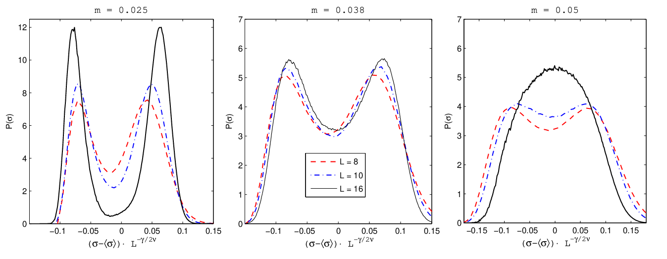
We now take full advantage of the worm algorithm and explore the chiral limit at fixed temperature in Fig. 4. As the quark mass is reduced, shifts to smaller values, and the transition becomes first-order, in qualitative agreement with expectations. The order of the transition can only be ascertained by a finite-size scaling study, which is illustrated in Fig. 5. For increasing mass values, the 3 panels each show the probability distribution of the chiral condensate for 3 spatial volumes. In each case, the distribution is reweighted to the pseudo-critical value of . The transition is clearly first-order for the smallest mass, and crossover for the largest. For the middle mass, an approximate data collapse is obtained by rescaling the condensate by , using and characteristic of the d Ising universality class. Indeed, for the U(1) chiral symmetry is broken explicitly, so we expect no special symmetry breaking other than to happen at the transition. Thus, we determine the critical endpoint for temperature to be approximately (see Fig.1). This can be compared with the mean-field prediction (Fig. 1) [5]. The discrepancy is an order of magnitude in !
5 Outlook and conclusions
We have presented first results of our study of
the strong coupling limit of lattice QCD at finite and .
The comparison with mean-field results and with the original Monte Carlo study
of Karsch et al. clearly justifies our project.
Algorithmic advances largely suppress the ergodicity problems of the
latter study, and lead to reliable, new estimates for over a range of masses.
The large discrepancy between exact Monte Carlo and approximate mean-field
determinations of the CEP at emphasizes the need for an exact
determination of the whole phase diagram. Quantitative mean-field results should be
considered with caution.
Our next step includes the determination of the phase diagram in the chiral
limit, and the introduction of asymmetric couplings to vary the temperature
continuously. As simulations in the chiral limit do not pose any problem for
a wide range of parameters, further topics of interest might include a detailed
comparison with chiral perturbation theory, and decay.
6 Acknowledgements
The work of M.F. was supported by ETH Research Grant TH-07 07-2.
References
- [1] F. Karsch and K. H. Mutter, Nucl. Phys. B 313 (1989) 541.
- [2] J. Hoek, N. Kawamoto and J. Smit, Nucl. Phys. B 199 (1982) 495.
- [3] H. Kluberg-Stern, A. Morel and B. Petersson, Nucl. Phys. B 215 (1983) 527.
- [4] P. H. Damgaard, N. Kawamoto and K. Shigemoto, Nucl. Phys. B 264 (1986) 1.
- [5] Y. Nishida, Phys. Rev. D 69 (2004) 094501 [arXiv:hep-ph/0312371].
- [6] N. Kawamoto, K. Miura, A. Ohnishi and T. Ohnuma, Phys. Rev. D 75 (2007) 014502 [arXiv:hep-lat/0512023].
- [7] K. Miura and A. Ohnishi, arXiv:0806.3357 [nucl-th]; N. Kawamoto, K. Miura and A. Ohnishi, arXiv:0710.1720 [hep-lat]; A. Ohnishi, N. Kawamoto and K. Miura, arXiv:0803.0255 [nucl-th].
- [8] G. Boyd, J. Fingberg, F. Karsch, L. Karkkainen and B. Petersson, Nucl. Phys. B 376 (1992) 199.
- [9] R. Aloisio et al., Nucl. Phys. B 564 (2000) 489 [arXiv:hep-lat/9910015].
- [10] P. de Forcrand and S. Kim, Phys. Lett. B 645 (2007) 339 [arXiv:hep-lat/0608012].
- [11] P. Rossi and U. Wolff, Nucl. Phys. B 248 (1984) 105.
- [12] N. Prokof’ev and B. Svistunov, Phys. Rev. Lett. 87 (2001) 160601.
- [13] D. H. Adams and S. Chandrasekharan, Nucl. Phys. B 662 (2003) 220 [arXiv:hep-lat/0303003].
- [14] F. Wang and D. P. Landau, Phys. Rev. Lett. 86 (2001) 2050.
- [15] P. de Forcrand and O. Philipsen, JHEP 0701 (2007) 077 [arXiv:hep-lat/0607017]; arXiv:0808.1096 [hep-lat].