Laboratori Nazionali di Frascati dell’INFN, Via E. Fermi 40, I-00044 Frascati, Italia \PACSes\PACSit11.30.ErCharge conjugation, parity, time reversal, and other discrete symmetries \PACSit12.15.HhDetermination of Kobayashi-Maskawa matrix elements \PACSit13.66.BcHadron production in collisions \PACSit14.40.Aq, K, mesons
Precision Kaon and Hadron Physics with KLOE
Abstract
We describe the KLOE detector at DAΦNE, the Frascati –factory, and its physics program. We begin with a brief description of the detector design and operation. Kaon physics is a major topic of investigation with KLOE thanks in part to the unique availability of pure ,, beams at a –factory. We have measured all significant branching ratios of all kaon species, the and lifetimes and the form factor’s dependence. From the measurements we verify the validity of Cabibbo unitarity and lepton universality. We have studied properties of light scalar and pseudoscalar mesons with unprecedented accuracy. We have measured the cross section necessary for computing the major part of the hadronic contribution to the muon anomaly. The methods employed in all the above measurements as well as the leptonic width, precision mass measurements and searches for forbidden or extremely rare decays of kaons and -mesons are described. The impact of our results on flavor and hadron physics to date, as well as an outlook for further improvement in the near future, are discussed.
1 Introduction
Late in 1989 the Istituto Italiano di Fisica Nucleare, INFN, decided to construct an collider meant to operate around 1020 MeV, the mass of the -meson. The -meson decays mostly to kaons, neutral and charged, in pairs. Its production cross section peaks at about 3 barns. Even with a modest luminosity, =100 b-1/s, hundreds of kaon pairs are produced per second. This collider, called a –factory and christened DAΦNE, is located at the Laboratori Nazionali di Frascati, LNF, INFN’s high energy physics laboratory near Rome [1].
1.1 DAΦNE
The DAΦNE layout is shown in fig. 1. The heart of the collider are two storage “rings” in which 120 bunches of electrons and positrons are stored. Each bunch collides with its counterpart once per turn, minimizing the perturbation of each beam on the other. Electrons and positrons are injected in the rings at final energy, 510 MeV. Electrons are accelerated to final energy in the Linac, accumulated and cooled in the accumulator and transferred to a single bunch in the ring. Positrons require first accelerating electrons to about 250 MeV to an intermediate station in the Linac, where positrons are created. The positrons then follow the same processing as electrons.
Since the stored beam intensities decay rapidly in time, the cycle is repeated several times per hour. A collider is characterized by its luminosity defined by: event rate=cross section, beam lifetime and beam induced radiation background.

The latter is large for short lifetimes, which also result in the average luminosity being smaller than the peak value, in a word, lower event yield and large, variable background. DAΦNE is housed in the ADONE building at LNF, see fig. 2.

DAΦNE runs mostly at center of mass energy . The meson decays dominantly to charged kaon pairs (49%), neutral kaon pairs (34%), (15%), and (1.3%). A factory is thus a copious source of tagged and monochromatic kaons, both neutral and charged. In most of the following we will assume that all analysis are carried out in the -meson center of mass. While this is in fact what we do, it is appropriate to recall that the electron and positron collide at an angle of -0.025 radians. The -mesons produced in the collisions therefore move in the laboratory system toward the center of the storage rings with a momentum of about 13 MeV corresponding to 0.015, 1.0001. mesons from -decay are therefore not monochromatic in the laboratory, fig. 3.
All discussion to follow refers to a system of coordinates with the -axis in the horizontal plane, toward the center of DAΦNE, the axis vertical, pointing upwards and the -axis bisecting the angle of the two beam lines. The momentum of neutral kaons varies between 104 and 116 MeV and is a single valued function of the angle between the kaon momentum in the laboratory and the -momentum, i.e. the -axis. Knowledge of the kaon direction to a few degrees allows to return to the -meson center of mass, fig. 3. The mean charged kaon momentum is 127 MeV.

1.2 KLOE
A state-of-the-art detector is needed to collect data at DAΦNE, from which physics results can be extracted. In summer 1991, the KLOE Collaboration was initiated proposing a detector and a program. The KLOE detector was not formally approved nor funded for another couple of years, because the authorities had not envisioned fully the magnitude of KLOE. By mid Summer 1998 however, KLOE was designed, constructed, completely tested and, complete with all of its electronics for signal processing, event gathering and transmission, was practicing with Cosmic Rays. Between Christmas and 1999 New Year, KLOE was moved from its own assembly hall onto the DAΦNE’s South Interaction Region.
The detailed KLOE saga, with its concomitant joys and travails, could be an entertaining tale that should be written up somewhere. Our purpose in this paper, is instead, chapter 2, to extract and describe those properties of the detector, chapter 3, its performance, and chapter 4, the special kaon “beams” available at DAΦNE, that made the physics measurements possible.
In the subsequent seven years KLOE, after beginning with a trickle of beam, by 2006 had produced data of such precision that the kaon, the first fundamental particle to introduce the concept of “flavor” into our current way of thinking, got its definitive 21st century portrait re-mapped with high precision, 60 years after its discovery. These are the subjects covered in the next chapters: chapter 5 details the new measurements of kaon physical parameters and decays; chapter 6, discusses the KLOE determination of of the CKM mixing matrix , unitarity and lepton universality tests, as well as search for new physics; chapter 7 is on quantum interferometry , and chapter 8 is on tests of CPT. Concurrently, capitalizing on the profuse production of light mesons resulting from electromagnetic transitions from the -mesons KLOE has improved scores of light meson properties often by orders of magnitude and these are discussed in chapter 9. Besides neutral kaon decays, symmetry tests have also been performed using light meson and charged kaon decays, see sections 9.1.2 9.4.2, and 5.3. Finally, utilizing initial state radiation KLOE has measured the dipion cross section, , over the whole range from the threshold to the mass energy, see chapter 10.
Most KLOE data were taken during two running periods. The 2001–2002 run yielded 450 pb-1 of data, corresponding to approximately 140 million tagged decays, 230 million tagged decays, and 340 million tagged decays. Analysis of this data set is essentially complete and most of the results are described in this report. KLOE also took data in 2004–2005, after completion of a number of DAΦNE modifications intended to increase the luminosity. About 2000 pb-1 were collected, giving a fivefold increase in statistics. In total, KLOE has collected during the years 1999 - 2005 2.5 fb-1 luminosity. Analysis of the 2004–2005 data is very advanced and prognosis of the improvements in accuracy in the measurements that are statistically limited are included either in the specific sections or in the final chapter 11.
2 Detector
The KLOE detector has a giant inner core, approximately 125 cubic meters, see fig. 4, and was built in Frascati in the KLOE assembly building, see fig. 5.

It is on the same scale and complexity as the “general purpose detectors” of its time that were operating at the world’s foremost laboratories such as LEP at CERN. If we consider that LEP operated at about one hundred times DAΦNE’s energy, producing much more energetic particles and with correspondingly greater multiplicities, KLOE’s large size would seem unwarranted. We shall see however that while KLOE’s complexity was necessitated by its intent of being a definitive high precision experiment, its size, instead, was dictated by the quirk of one of the two neutral kaons, called the , of living an extraordinarily long time (for a short lived particles) , about 51 nanoseconds. Kaons from -mesons decaying at rest, travel at approximately one fifth of the speed of light. This low speed is a great bonus for many reasons. However the mean path travelled by a -meson, is 3.4 m. Thus if we want a detector which can catch =63% of all decaying neutral long-lived kaons, it must have a radius of some three and a half meters. We compromise on two meters and catch some 40% of those decays. Less than that in fact, since some volume is inevitably lost around the beam interaction point, IP, and some more is lost at the outer edge, in order to be able to recognize the nature of the decays close to it.
The major components of KLOE that enclose the decay volume around the IP are, going outwards radially, a large tracking device to reconstruct the trajectory of charged particles, the Drift Chamber DC, surrounded by a hermetic calorimeter to measure the energy and the entry point of photons, the Barrel EMC and two End-cap EMC. The tracking chamber and the calorimeter are immersed in a mostly axial magnetic field of 0.52 T, provided by a superconducting coil enclosed in its iron yoke.

2.1 Drift Chamber
In the design of the KLOE tracking chamber one is constrained by the desire to catch all the charged secondary products from a decay and measure their properties with great precision, without jeopardizing the need to achieve the same for the neutral secondary products. Recalling that when a charged particle travels in a medium, a gas, it undergoes repeated collisions with electrons, releasing part of their energy, resulting in a string of ion pairs created marking its passage. Thus when the particle enters a drift chamber, DC (a gas filled chamber traversed by a large number of wires, some kept at +2000 volt, anode wires, some at ground), electrons of the ion pairs created along its trajectory drift to the positive voltage wires and from an avalanche multiplication mechanism a detectable signal appears at the wire’s end. KLOE custom designed sophisticated electronics that are mounted at the wire’s end which senses the tiny signals and provide us with the drift charge and time measurement. Furthermore, the total integrated charge collected at the wire’s end gives information on the energy released from the initial particle.
Furthermore, particles of different mass travelling in the same medium and with the same momenta have different energy releases: for the same they have different and approximately the specific ionization . Therefore this information is suitable to perform particle identification (PID). Finally, measuring the drift time locates the distance of the track from the anode wires which is then used to reconstruct the trajectory of the particles.
A caveat, the actual path of the particle is altered by multiple scattering, the multiple scattering angle being , where is the radiation length which is roughly proportional to , in gr/cm2 (and one must not forget the density). Finally, while moving towards the anode, the drifting ionization undergoes diffusion, the amount of which is a function of the density of the gas mixture of the DC.
After judicious balancing, in order to avoid the regenerations ( generated from the strong interaction of a with the traversed medium that might simulate CP-violating decays), a helium based gas mixture was chosen to minimize multiple scattering and density, despite the fact diffusion of drifting ionization is larger in He than certain other gases. The average value of the radiation length in the DC volume is m, including the wire’s contribution.
Again, for the mechanical structure low- and low density materials were used to minimize regeneration, tracks’ multiple coulomb scattering and the absorption of photons before they can reach the calorimeter. To achieve this the chamber is constructed out of a carbon fiber composite. The chamber volume is delimited by an outer cylinder of 2 m radius, an inner cylinder of 25 cm radius and closed by two 9 mm thick annular endplates 9.76 m radius of curvature and a 25 cm radius hole in the center. Due to their large size, the endplates were fabricated in two halves then glued together. About 52,000 holes were drilled on each endplate for the insertion of the feedthroughs holding the DC wires. The total axial load on the end plates, about 3500 kg, would deform the end plates by several mm at the end of stringing. The deformation problem was solved by using rings of rectangular cross-section which surround the L-shaped plate rims, made of the same material. The ring is used to apply a tangential pull to the spherical plate via 48 tensioning screws made of titanium alloy pulling on tapped aluminum inserts in the L-shaped flange. The net result of the pull is to approximate a complete sphere beyond the outer edge of the plate which greatly reduces the deformation. Each screw was instrumented with two strain gauges, calibrated in order to compensate for bending effects on the screws, so that the pulling force was always known. At the end of stringing the deviation from the spherical shape of the endplates was measured to be less than 1 mm and the hole positions to be accurate at the level of 60 m. The KLOE DC is indeed a tour de force achievement thereafter copied in other experiments (albeit never to the same large dimensions).
The KLOE DC [2] has 52,000 wires, about 12,500 of them are sense wires, the remaining ones shape the electric field in 12,500 almost square cells located on cylindrical layers around the -axis (defined by the bisector of the two crossing beams). Particles from the decays are produced with small momenta and therefore track density is much higher at small radii. This motivated the choice of having the 12 innermost layers made up of cm2 cells and the remaining 48 layers with cm2 cells. For a particle crossing the entire chamber we get dozens of space points from which we reconstruct a track: the track of a pion from decay has 60 space points in average. An all stereo geometry allows the measurement of the coordinate. Fig. 6 shows the wire geometry during the DC construction as illuminated by light. In this particular arrangement, shown in fig. 7 left, the wires form an angle with the -axis, the stereo angle . Consecutive layers have alternating signs of this angle and its absolute value increases from 60 to 150 mrad with the layer radius while keeping fixed for all the layers the difference between and distances (1.5 cm), defined in fig. 7 left.

This design results in a uniform filling of the sensitive volume with almost-square drift cells, with shape slowly changing along , which increases the isotropy of the tracking efficiency.
To extract the space position from the measured drift time of the incident particle, we need to know the space-time relation describing the cell response. The whole DC can be described using 232 space-time relations only, parametrized in terms of the angles and defined in fig. 7 right. The angle characterizes the geometry of the cell, directly related to the electric field responsible of the avalanche multiplication mechanism. The angle gives the orientation of the particle trajectory in the cell’s reference frame, defined in the transverse plane and with origin in the sense wire of the cell.


The presence of a signal on a wire and its drift time and distance is called hit. Once we have the hits, we can proceed with the event reconstruction using the wire geometry, space-time relations and the map of the magnetic field. This procedure follows three steps: (i) pattern recognition, (ii) track fit, and (iii) vertex fit. The pattern recognition associates hits close in space to form track candidates and gives a first estimate of the track parameters. Then track fit provides the final values of these parameters minimizing a function based on the difference between the fit and the expected drift distances, residuals, as evaluated from a realistic knowledge of the cells’ response (measured drift times and space-time relation). This is an iterative procedure because the cells’ response depend on the track parameters. Finally the vertex fit searches for possible primary and secondary vertices, on the basis of the distance of closest approach between tracks.
Besides the drift time and position information, hits in the DC are also associated to a charge measurement directly related to the energy released in the cell from the incident particle. The amount of collected charge depends on the particle’s track length in the crossed cell. The energy deposited in a sample of finite thickness fluctuates and exhibits a Landau distribution, with a long tail at high energies. Therefore to improve the energy resolution, the energy deposited is sampled many times for each track and a truncated mean technique is used. To use the charge information for particle identification purposes it is necessary to normalize the charge to the track length and define the specific ionization dE/dx. If the energy is measured in counts, we have on average 15 counts/cm for pions and muons from and decays, with momentum within 180 and 300 MeV. Instead tracks exhibit a larger number, 120 counts/cm.
The drift chamber provides tracking in three dimensions with resolution in the bending plane better than 200 m, resolution on the measurement of 2 mm and of 1 mm on the decay vertex position.The particle’s momentum is determined from the curvature of its trajectory in the magnetic field with a fractional accuracy better than 0.4% for polar angles larger than 45∘. The calibration of the absolute momentum scale has a fractional accuracy of few using several two- and three-body decays (,, , , ,) covering a wide momentum range. Deviations from nominal values of invariant mass, missing mass or momentum of the charged decay particle in the rest frame of the decaying particle are used as benchmarks for the calibration procedure. The resolution on the specific ionization measurement obtained using two- and three-body decays and Bhabha scattering events, is for pions and for electrons [3], using 60 truncated samples.
The DC system’s complexity, as well as the demands placed upon it requires the response of each cell to an incoming particle to be known accurately. The cell response is a function of its geometry and of the voltage applied to the wires. Thus the position of the DC, mechanical structure as well as wires, had to be surveyed, in situ, together with the other KLOE components.
The Slow Control monitoring system (sect. 2.6) fully embedded in the Data Acquisition process (sect. 2.5), sets and registers the voltages applied to the wires, sends the information to the read-out electronics and controls its proper functioning [4]. Moreover the gas mixture parameters, namely composition, temperature and pressure, enter directly in the space-time relations used in reconstructing the particle trajectory, to extract the space position from the measured drift time of the incident particle. The Slow Control System also monitors the gas parameters.
To ensure the stability in time of the DC performance, the system has to be calibrated periodically by acquiring samples of cosmic-ray muons suitable for the measurement of the 200 different space-time relations. The calibration program, incorporated into the KLOE online system, automatically starts at the beginning of each run and selects about 80,000 cosmic-ray events. These events are tracked using the existing space-time relations and the average value of the residuals for hits in the central part of the cells is monitored. If the residuals exceed 40 m then about 300,000 cosmic-ray events are collected, with about 30 Hz rate, and a new set of calibration constants is obtained. At the beginning of each data-taking period a complete calibration of the space-time relations is needed together with the measurement of the DC time offsets, the latter from some 107 cosmic-ray events. Finally, during data taking the DC performances are monitored using selected samples of Bhabha scattering events.
2.2 Electromagnetic Calorimeter
The neutral decay products of the ’s, its short-lived partner (lifetime 89 picoseconds) and of those of their charged brethren, the ’s, which we need to detect, are photons, either directly produced or from the decay of neutral pions into two photons. It is important to recall that photons for energies larger than a few MeV, as in most of our cases, interact with matter by electron positron pair production that in turn radiate photons when traversing matter, a process quite similar to pair-production. Thus, a photon, or an electron for that matter, travelling through dense, high matter, repeatedly undergoes radiation and pair production in cascade, until all its energy is expended in a so called shower of and photons. From detection of these particles and their energy one measures the original photon’s (or electron’s) energy. This is done with a “calorimeter”, which also usually pinpoints the position of the electromagnetic cascade (or shower) as well.
The KLOE calorimeter, EMC, has been designed and built to satisfy a set of stringent requirements such as providing a hermetic detection of low energy photons (from 20 to 500 MeV) with high efficiency, a reasonable energy resolution and an excellent time resolution to reconstruct the vertex for the neutral decays. The calorimeter response has also to be fast since its signals are used to provide the main trigger of the events.
The chosen solution for the EMC is that of a sampling calorimeter, composed of lead passive layers, accelerating the showering process, and of scintillating fiber sensing layers. It is made of cladded 1 mm scintillating fibers sandwiched between 0.5-mm-thick lead foils. The foils are imprinted with grooves wide enough to accommodate the fibers and some epoxy, without compressing the fibers. This precaution prevents damage to the fiber-cladding interface. The epoxy around the fibers also provides structural strength and removes light travelling in the cladding. In more detail, the basic structure of 0.5 mm, grooved Pb layers between which are embedded 1 mm diameter scintillating fibers are positioned at the corners of almost equilateral triangles. 200 such layers are stacked, glued, and pressed, resulting in a bulk material. The resulting composite has a fibers:lead:glue volume ratio of 48:42:10 which corresponds to a density of 5 g/cm3, an equivalent radiation length of 1.5 cm and an electromagnetic sampling fraction of 13%. The large ratio of active material to radiator, the frequent signal sampling and the special fiber arrangement result in a factor improvement in energy resolution with respect to calorimeter with slabs of equivalent scintillator:lead ratio. The chosen fibers, Kuraray SCSF-81 and Pol.Hi.Tech. 00046, are blue emitting scintillating fibers with a fast emission time whose larger component is described by an exponential distribution with a of 2.5 ns. In addition, the special care in design and assembly of the Pb-fiber composite ensures that the light propagates along the fiber in a single mode, resulting in a greatly reduced spread of the light arrival time at the fiber ends. Propagation speed in the fiber is 17 cm/ns. These fibers produce more than 5 photons for one MeV of deposited energy by ionizing particles. 3% of the light reaches the fiber ends. Fibers transmit 50% of the light over 2 m (m).
This material is shaped into modules 23 cm thick (). 24 modules of trapezoidal cross section are arranged in azimuth to form the calorimeter barrel, aligned with the beams and surrounding the DC. An additional 32 modules, square or rectangular in cross section, are wrapped around each of the pole pieces of the magnet yoke to form the endcaps, which hermetically close the calorimeter up to 98% of 4, see fig. 8. The unobstructed solid-angle coverage of the calorimeter as viewed from the origin is 94% [5].

The fibers run parallel to the axis of the detector in the barrel, vertically in the endcaps, and are read out at both ends viewed by lucite light guides of area of 4.44.4 cm2. The other end of the guides are coupled to the photocathodes of fine mesh photomultipliers of 1.5 inches diameter with quantum efficiency of 20%. The fiber length of 4 m corresponds to an average photoelectron yield of 35 p.e./layer for a minimum ionizing particle crossing the calorimeter at the fiber center. The photomultiplier tubes at each fiber’s end transform the light into electric pulses. Their amplitudes, , is proportional to the amount of energy deposited while the recorded times, , are related to the time of flight of the particle. For each cell the position of the readout elements and the difference of the arrival times at the two fiber ends determine the shower position with a (1) cm accuracy. The full stack of 23 cm (15 ) fully contains a shower of 500 MeV. 4880 photomultiplier tubes view the 24+32+32 modules into which the calorimeter is subdivided for a grand total of 15,000 km used optical fibers.
As a first step, the reconstruction program makes the average of time and energy of the recorded and for the two sides of each cell and compute the hit position. Corrections for attenuation length, energy scale, time offsets and light propagation speed are taken into account at this stage. A clustering procedure then groups together nearby clumps of energy deposition and calculates the average quantities over all the participating cells. The calibration constants to transform and from raw quantities to time in nanoseconds and energy in MeV are evaluated with dedicated on-line and off-line algorithms.
The energy calibration starts by a first equalization in cell response to minimum ionizing particles (m.i.p) at calorimeter center and by determining the attenuation length of each single cell with a dedicated cosmic ray trigger. This is done before the start of each long data taking period. The determination of the absolute energy scale in MeV relies instead on a monochromatic source of 510 MeV photons: the sample. This last calibration is routinely carried out each 200- 400 nb-1 of collected luminosity.
For the timing, the relative time offsets of each channel, , related to cable lengths and electronic delays and the light velocity in the fibers are evaluated every few days with high momentum cosmic rays selected with DC information. An iterative procedure uses the extrapolation of the tracks in the calorimeter to minimize the residuals between the expected and measured times in each cell. A precision of few tens of picoseconds is obtained for these offsets.
To run at the design luminosity, DANE operated with a bunch-crossing period equal to the machine radio frequency (RF) period, ns. Due to the spread of the particle’s arrival times, the trigger is not able to identify the bunch crossing related to each event, which has to be determined offline. The start signal for the electronics devoted to time measurement (TDC) is obtained by phase-locking the trigger level-1 signal (sect. 2.4) to an RF replica, with a clock that has a period of . The calorimeter times are then related to the time of flight of the particle from IP to the calorimeter, , by , where is a single number accounting for the overall electronic offset and cable delay, and is the number of bunch-crossings needed to generate the TDC start. The values of and are determined for each data taking run with events by looking at the distribution of where is the expected time of flight: well separated peaks correspond to different values of . We arbitrarily define as the position of the peak with the largest statistics, and determine from the peaks’ distances. Both quantities are evaluated with a precision better than 4 ps for 200 nb-1 of integrated luminosity. This measurement of allows us to set the absolute calorimeter time scale to better than 0.1 %. During offline processing, to allow the cluster times to be related to the particle time of flight, we subtract and determine, on an event by event basis, the “global” event start time , i.e. the quantity . A starting value for all analysis is evaluated by assuming that the earliest cluster in the event is due to a photon coming from the interaction point. Further corrections are analysis dependent.
The high photon yield and the frequent sampling enable cluster energies to be measured with a resolution of , as determined with the help of the DC using radiative Bhabha events. The absolute time resolution is dominated by photoelectron statistics, which is well parametrized by the energy scaling law. A constant term of 140 ps has to be added in quadrature, as determined from , radiative decays and data control samples. This constant term is shared between a channel by channel uncorrelated term and a common term to all channels. The uncorrelated term is mostly due to the calorimeter calibration while the common term is related to the uncertainty of the event , arising from the DAΦNE bunch-length and from the jitter in the trigger phase-locking to the machine RF. By measuring the average and the difference of for the two photons in events, we estimate a similar contribution of 100 ps for the two terms. Cluster positions are measured with resolutions of 1.3 cm in the coordinate transverse to the fibers, and, by timing, of in the longitudinal coordinate. These performances enable the vertex in decays to be localized with cm along the line of flight, as reconstructed from the tagging decay. Incidentally, the thin lead layers used and the high photon yield allows high reconstruction efficiency for low energy photons.
2.3 Beam Pipe and Quadrupole Calorimeter
At DAΦNE the mean , and decay path lengths are cm, m and cm. To observe rare decays and interference with no background from regeneration, a decay volume about the interaction point with must remain in vacuum. The beam pipe, see fig. 9, surrounds the interaction point, with a sphere of 20 cm inner diameter, with walls 0.5 mm thick made of a Be-Al sintered compound. This sphere provides a vacuum path the amplitude decay length, effectively avoiding all regeneration.

Permanent quadrupoles for beam focusing are inside the apparatus at a distance of 46 cm from IP, and surrounding the beam pipe. The quadrupoles of this low- insertion are equipped with two lead/scintillating-tile calorimeters, QCAL, of thickness, with the purpose of detecting photons that would be otherwise absorbed on the quadrupoles [6]. Specifically, the QCAL main task is to identify and reject photons from decays when selecting the CP violating events. Each calorimeter consists of a sampling structure of lead and scintillator tiles arranged in 16 azimuthal sectors. The readout is performed by plastic optical fibers, Kuraray Y11, which shift light from blue to green (wavelength shifter, WLS), coupled to mesh photomultipliers. The special arrangement of WLS fibers allows also the measurement of the longitudinal coordinate by time differences. Although the tiles are assembled in a way which maximizes efficiency for photons, a high efficiency is in fact also obtained for photons coming from the IP. This allows us to extend the EMC coverage of the solid angle down to =0.99 for prompt decays. The time resolution is related to the light yield and emission time/photoelectron of the Kuraray Y11 fibers. For a m.i.p. crossing the whole stack of 16 tiles, we had obtained during tests a light yield of 50 photoelectrons for entry points close to the PM’s side. Considering that a m.i.p. deposits an energy equivalent to that of a 75 MeV photon, this corresponds to p.e./MeV and in turn implies a time resolution for electromagnetic showers of 205 ps. However during running, the presence of the B-field reduces the effective light yield by a factor 1.4, thus worsening the timing to 240 ps, which however is high enough to yield an efficiency above 90% for photon energies greater than 20 MeV.
2.4 Trigger
Event rates at DAΦNE are high; at the maximum luminosity of cm-2s-1 up to s-1 and Bhabha s-1 are produced within the KLOE acceptance window. The trigger design [7] has been optimized to retain all decays. Moreover, all Bhabha and events produced at large polar angles are accepted for detector monitoring and calibration, as well as a downscaled fraction of cosmic-ray particles, which cross the detector at a rate of Hz. Finally, the trigger provides efficient rejection on the two main sources of background: small angle Bhabha events, and particle lost from the DAΦNE beams, resulting in very high photon and electron fluxes in the interaction region.
The trigger electronic logic system rapidly recognizes topologies and energy releases of interest, processing the signals coming both from EMC and DC. Since decay events have a relatively high multiplicity, they can be efficiently selected by the EMC trigger by requiring two isolated energy deposits (trigger sectors) in the calorimeter above a threshold of 50 MeV in the barrel and 150 MeV in the endcaps. Events with only two fired sectors in the same endcap are rejected, because this topology is dominated by machine background. Moreover, events with charged particles in the final state give a larger number of hit wires in the DC than do background events. The DC trigger employs this information, requiring the presence of 15 hits in the DC within a time window of 250 ns from beam crossing. An event satisfying at least one of the two above conditions generates a first level trigger, T1, which is produced with minimal delay and is synchronized with the DAΦNE master clock. The T1 signal initiates conversion in the front-end electronics modules, which are subsequently read out following a fixed time interval of s, which is ultimately driven by the typical drift distances travelled by electrons in the DC cells. In case of DC trigger, a validation of the first level decision is required by asking for 120 hits within a 1.2-s time window.
The KLOE trigger also implements logic to flag cosmic-ray events, which are recognized by the presence of two energy deposits above 30 MeV in the outermost calorimeter layers. For most data taking, such events were rejected after partial reconstruction by an online software filter.
2.5 Data acquisition and processing
At a luminosity of 100 b-1/s, the trigger rate is 2000 Hz. Of these 500 Hz are from decays or Bhabha scattering. All digitized signals from the calorimeter, drift chamber, calibration and monitoring systems are fed via fiber optics from the electronics, sitting on platforms mounted on the KLOE iron yoke, to the computers in the next building. The Data Acquisition architecture has been designed to sustain a throughput of 50 Mbytes/s all along this path. In the near-by control room one can see real time displays of reconstructed charged tracks traversing the DC and photons depositing energy clusters in the EMC. The display of two events is shown in fig. 10.
The events are reconstructed, meaning that charged tracks and energy deposits that occurred at the same instant in time on the various subcomponents of KLOE are associated together, properly labelled and packed into a unique file. To optimize the event reconstruction we use continuously updated calibration constants for the time and energy scales. Furthermore, background hits are acquired using a random trigger, which are recorded in order to be used in the simulation of KLOE events (MC). The MC simulation program reproduces accurately the detector geometry, the response of the apparatus and the trigger requirements , but of course cannot foretell the moment to moment variation of the background.
All raw data, background, reconstructed and MC events are recorded on tape. KLOE has a huge tape library of 800 TB capacity [4]. At reconstruction time, events are classified into broad categories, or “streams”. Data summary tapes are produced with a separate procedure.


Any of the KLOE analyses, even after event reconstruction is quite complex. It includes making data summary tapes and extensive modelling of the detector response. This requires generation of large number of Monte Carlo (MC) events for each process under study. “Offline” processes run in a farm of computers of 150 kSPECint2K CPU power, all residing in the dedicated computer center. Both data and MC summaries (80 TB) are cached on disk for analysis [8].
2.6 Slow control system
KLOE has to be operated 24 hours a day, 7 days a week. Therefore it has to be kept under continuous control, both to guarantee efficient data taking, and for safety reasons. Parameters such as high and low voltage settings, the temperature of the electronics components, or the status of the drift chamber gas system are set and monitored by a dedicated system fully embedded in the Data Acquisition process: the Slow Control.
This system also records some machine parameters, and provides to the DAΦNE team information about KLOE including our on line measurements of the luminosity and of the background levels.
3 Reconstruction Performances
KLOE provides a continuous monitoring of the machine working point, providing feedback to DAΦNE continuously as well. The most important parameters are the beam energies and crossing angle, which are obtained from the analysis of Bhabha scattering events with polar angles above 45 degrees. The average value of the center-of-mass energy is evaluated online during data taking with a precision of keV for each 200 nb-1 of integrated luminosity. This determination is further refined with offline analysis to achieve a precision of keV, as discussed later. The position of the primary vertex, with coordinates , , and , is reconstructed run-by-run from the same sample of Bhabha events. and are determined with typical accuracy of about m, and have widths and which are about mm and few tens of microns, respectively. is also reconstructed online with m accuracy, but it has a natural width of mm, determined by the bunch length itself.
3.1 Overview of EMC and DC performances
We note that while KLOE is a general purpose apparatus with good performances of the two main detectors, the DC and the EMC, its real strength manifests when joining the reconstruction capability of both detectors. To give an overall view at a glance, we first summarize in table 1 the parametrized resolution for neutral particles (mainly photons) and for charged tracks (mainly electrons/pions) for prompt decays and ,. Resolution on invariant masses are also reported in the same table as well as the reconstruction capability for neutral and charged vertices.
| EMC | DC | ||
| parametrization | parametrization | ||
| 5.7% | % | ||
| (MeV) | 15 (), 40 (,K) | (MeV) | 1 (,K) |
| (cm) | 1.3 | (m) | 150 |
| (cm) | 1.2 | (mm) | 2 |
| (ps) | 57 + 140 | 120 (K±), 15 ( from ) | |
| (cm) | 2-3 | (mm) | 2 (@IP), 3 (@L 1m) |
In KLOE, the single particle reconstruction efficiency can be determined from data control samples, as well as from Monte Carlo simulation. As an example, the photon reconstruction efficiency as a function of the photon energy can be estimated from events, where a redundant determination of the decay photon kinematics is possible using the charged pion momenta as measured from the DC. For charged particles produced at the interaction point, the track efficiency can be measured from events selected with the requirement of having at least one track fulfilling the two-body decay kinematics. A high reconstruction efficiency is observed for both detectors on data and Monte Carlo. For each specific analysis, the event selection efficiency is evaluated from Monte Carlo. To take into account data-MC difference in the cluster/track efficiencies, the calculation is usually performed by weighting each particle in the final state with the ratio of data/MC reconstruction efficiencies.
For particle identification, PID, we start extrapolating tracks on the calorimeter surface and associating tracks to clusters. The identification of photons is based on clusters not associated to any track and on the difference between expected and reconstructed time of flight, ToF, for straight trajectories. The PID of charged tracks, which at the considered energy are electrons, pions and muons, is based on a combined usage of EMC and DC, by looking at ToF, and cluster shape. At low momenta, MeV, the ToF is usually the winning handle while at higher momenta variables based on cluster shape are used. Often these information are combined together in a likelihood identification variable [9] or using a neural network [10]. To identify charged kaons we can use instead dE/dx, given the excellent separation provided by the specific ionization measurement between kaons and the other charged particles produced in the apparatus.
3.2 Absolute energy scale
An improved determination of the center-of-mass energy, , is obtained for each run by fitting the invariant-mass distribution for Bhabha events to a Monte Carlo generated function, which includes radiative effects. Initial state radiation (ISR), where one or both initial colliding particles radiate a photon before interacting, affects the center-of-mass energy and therefore the final state invariant mass. The ISR is mostly collinear to the beam, and in general is not detected. MC Bhabha events were generated using the Babayaga [11] event generator, which accounts for both final and initial state radiation.
The absolute energy scale is calibrated by measuring the visible cross section for the process. The cross section peak is fitted to a theoretical function [12], which depends on the parameters, takes into account the effect of ISR, and includes the interference with the and the mesons. The mass, total width, and peak cross section are the only free parameters of the fit, the and the parameters being fixed. The results of the fit to the data are shown in fig. 11. The mass value obtained from the fit is MeV, which has to be compared with MeV, measured by CMD-2 at VEPP-2M [13]. For CMD-2 the absolute energy scale is accurately determined from beam induced resonant depolarization, so that we use the ratio / to correct our determination of the center of mass energy. This corresponds to a shift in the value of of 150 keV.


3.3 Luminosity
The tagging capability of the calorimeter trigger allowed us to perform fast luminosity measurements, providing a robust estimate of the DAΦNE luminosity with few per cent accuracy. This was achieved by counting Bhabha events in the acceptance of the calorimeter barrel. For this purpose, we selected events with two trigger sectors fired on the barrel, imposing a higher discrimination threshold than the one used in the standard acquisition chain. The tight angular selection, which reduces the available statistics by a factor of , was motivated by the need to keep under control the overwhelming machine background, which is concentrated at small angle. Additional cuts on the position of the fired sectors and on the time difference between the two signals were added to improve rejection on the residual background, from cosmic-ray events. When operating at =100 b-1/s, the luminosity measurement was updated every 15 s, with a statistical error of 3%. Fig. 12 top shows the monthly integrated luminosity by KLOE since January 2001, while in the bottom the year integrated luminosity is shown. These data have been collected almost exclusively at the peak. In early 2006, KLOE also collected 200 pb-1 of data at MeV, at which drops to 5% of its peak value.


Finally, it is important to note that already in year 2000 KLOE collected 20 pb-1, producing quite a few publications which improved the knowledge in both hadronic and kaon physics [14, 15, 16, 17, 18].
A more accurate measurement of the integrated luminosity is performed offline [19], using Bhabha events in the polar angle range , the so-called VLAB events. The effective cross section for these events, nb, is large enough to reduce the statistical error at a negligible level. The luminosity is obtained by counting the number of VLAB candidates, , and normalizing it to the effective Bhabha cross section, , obtained from MC simulation, after subtraction of the background, :
| (1) |
The precision of the measurement depends on the correct inclusion of higher-order terms in computing the Bhabha cross section. For this purpose we use Babayaga, which include the QED radiative corrections in the framework of the parton-shower method. The quoted precision is 0.5%, although an updated version of this generator, Babayaga@NLO [20], has been released recently. The new predicted cross section decreased by 0.7% and the theoretical systematic uncertainty improved from 0.5% to 0.1%.
The VLAB events are selected with requirements on variables that are well reproduced by the KLOE MC. The acceptance cut on the electron and positron polar angle, is based on the calorimeter clusters, while the momentum selection, MeV, is based on the DC determination. The background from , , and events is well below and is subtracted. All selection efficiencies (trigger, cluster and track reconstruction) are greater than , as obtained from MC and confirmed with data control samples. Finally, corrections are applied on a run-by-run basis to follow the small variations in the center-of-mass energy and in the detector calibration. In the end, we quote a 0.3% uncertainty in the determination of the acceptance due to experimental effects.
4 Kaon beams
The neutral kaon pair from is in a pure state. Therefore the initial two-kaon state can be written, in the -rest frame, as
|
|
(2) |
where the identity holds even without assuming invariance. Detection of a thus signals the presence of, “tags”, a and vice versa. Thus at DAΦNE we have pure and beams of precisely known momenta (event by event) and flux, which can be used to measure absolute and branching ratios. In particular DAΦNE produces the only true pure beam and the only beam of known momentum. A beam permits studies of suppressed decays without overwhelming background from the component. A beam allows lifetime measurements. Similar arguments hold for and as well, although it is not hard to produce pure, monochromatic charged kaon beams. In the following sections we briefly discuss the criteria adopted to tag the , , and charged kaon beams.
4.1 beam
Because of the exceptional timing capabilities of the EMC and the slowness of the kaons from -decays, we use a ToF technique to tag -mesons in a unique way. As already mentioned, neutral kaons have a velocity in the frame and =0.193 to 0.239 in the lab, and 60% of them reach the calorimeter in a time 31 ns. -mesons interact in the calorimeter with an energy release up to their mass, 497 MeV. For an energy release of 100 MeV we have a time resolution of 0.3 ns, i.e. about a 1% accuracy on velocity, shown in fig. 13.

In KLOE, we call a interaction in the EMC a “K-crash”, and we use it as a tag for the . Note that the above error on () corresponds to an error on the kaon energy of 0.25 MeV or 1 MeV for its momentum, with just one event. Adding the information about the position of the energy release, the direction of the line of flight is determined with angular accuracy. Using the previous value of momentum, and the run-average value of the momentum as evaluated from Bhabha events, we determine the momentum from , with the same accuracy as for .
4.2 beam
All of the produced mesons decay within few centimeters from the interaction point. Therefore, in principle, all of them can be detected in the apparatus. On the contrary, ’s can travel several meters before decaying, thus escaping detection. From the above, it follows that a pure sample of nearly monochromatic ’s can be selected by identification of decays. The best performances in terms of efficiency and momentum resolution are obtained by selecting decays. These are identified as two-track vertices close to the interaction point, with invariant mass in a 5 MeV acceptance window around the nominal kaon mass. The decay provides also a good measurement of momentum, , where is again the momentum as determined from Bhabha scattering events. The resolution is 0.8 MeV on the momentum, while the flight direction is determined within .
More interestingly, events with both a decay and a K-crash identified allow us to measure the DAΦNE beam energy spread. This is extracted by comparing for each event the two independent determinations of center-of-mass energy that are evaluated using the and momenta, respectively. Using this technique we find a beam energy spread of 220 keV, in agreement with the machine model expectation.
For many KLOE measurements, it is of fundamental importance to accurately determine the exact amount of lost/retained decays, or, in other words, determining the decay fiducial volume. For decays involving two charged particles this is obtained relatively easily by the observation of the vertex of the two related tracks in the drift chamber, measured with an accuracy of 3 mm. The task is more difficult for totally neutral decay channels, but can still be achieved using the excellent timing accuracy of the EMC. As an example, we can locate the decay point, the “neutral vertex”, with accuracies of cm, as illustrated in fig. 14, left.


Each photon from the decay point (D) defines a time-of-flight triangle: the first side is the segment from the interaction point to the decay vertex (ID); the second is the segment from the decay vertex to the centroid of the calorimeter cluster (DA); and the third is the segment from the interaction point to the cluster centroid (IA). The direction is initially known, because the decay is tagged. The photon vertex position is specified by the distance ID, which is determined from
| (3) |
where is the cluster time and is the velocity. The position of the interaction point is obtained by backward extrapolation along the flight path. The decay vertex position is evaluated for each neutral cluster separately, and the energy-weighted average of the values for each cluster is then taken as its final determination. The accuracy in the location of the photon vertex has been studied using decays, in which the decay position can be independently determined using clusters and tracks, with much greater precision in the latter case. The dependence of the position resolution on decay distance () is illustrated in fig. 14, right.
4.3 beam
The -meson decays 50 of the times into pairs; these are quasi anti-collinear in the laboratory, due to the small crossing angle of the e+e- beams, with momentum ranging between 120 and 133 MeV/c and decay length cm. While moving towards the DC volume, the average momentum decreases to 100 MeV/c due to the energy loss in the beam pipe and DC inner wall materials. As for neutral kaons, the identification of a decay tags a beam with known flux, thus giving the possibility to measure kaon absolute branching ratios. Charged kaons are tagged using their two-body decays, and , accounting for 85% of the total decay channels. These decays are observed as “kinks” in a track originating at the IP. The charged kaon track must satisfy MeV/c. The momentum of the decay particle in the kaon rest frame evaluated using the pion mass, , is 205 and 236 MeV, for decays to and , respectively. Fig. 15 shows the distribution obtained assuming the decay particle is a pion. Cutting on the spectrum of the decay particle, we select about events/pb-1 of integrated luminosity.

5 Kaon physical parameters and decays
Since the kaon’s discovery about sixty years ago, knowledge of its properties, from masses, lifetimes, and how often each species decays into to which particles (the so called branching ratios, BR), has been accumulated piecemeal literally over hundreds of individual experiments, performed at various laboratories all over the world. Each experiment has its own peculiarity, contingent upon the particle beam available and its own equipment’s acceptance range, which can result in highly accurate measurements from a statistical point of view (namely based on thousands of data events) but with hidden corrections peculiar to it perhaps unknown even to its authors. The particle data group [21] in charge of compiling the results, often adopt a “democratic” way of weighing the various results according to their nominal errors and literally applying a scale factor to these errors when faced with two inconsistent measurements. This procedure skirts the problems of judging the validity of results obtained over time and sometimes ends up with a hodge-podge of inconsistent results forced into a mold of dubious scientific validity.
The mission of KLOE is to measure most, if not all, of the properties of the kaon system to high accuracy, with a single detector simultaneously. One problem that consistently plagues the interpretation of older measurements is the lack of clarity about accounting for radiative contributions. All of our measurements of kaon decays with charged particles in the final state are fully inclusive of radiation. Radiation is automatically accounted for in the acceptance correction. All our MC generators incorporate radiation as described in [22].
Because of the availability of tagged and pure kaon beams of known momenta, KLOE is the only experiment that can at once measure the complete set of experimental inputs, branching ratios, lifetimes and form factor parameters for both charged kaons and long lived neutral kaons. In addition KLOE is the only experiment that can measure branching ratios at the sub-percent level.
5.1 Mass
Kaon masses are about 500 MeV, very close to one half the -meson mass, known to an accuracy of 0.019/1019.460 by the use of the -2 depolarizing resonances, [21]. The events offer a unique possibility to obtain a precise value of the neutral kaon mass. Indeed we observe that if the -meson is at rest the kaon mass can be extracted from the kaon momentum using the relation:
| (4) |
Since MeV, measuring it at 1% level, well within the KLOE capability, results in a measurement of the mass better than %. 50,000 events are enough to reach a statistical accuracy of about 1 keV.
mesons are produced with a momentum along the axis, MeV at DAΦNE. From the measured momenta of the two pions from , we measure the momentum. The momentum is given by , where is the average momentum measured with Bhabha events collected in the same runs. The center of mass energy of the pair () is related to the kaon mass , according to:
with
On the other hand the collision center of mass energy is computed from Bhabha events, as described in sect. 3.
Corrections due to ISR have to be taken into account when relating to . The correction function has been evaluated using a full detector simulation where the radiation from both beams has been implemented, and is reconstructed as in the data. The expression of the radiator function has been taken from [23], including corrections. The correction is very small below the resonance, corresponding to a shift in of 40 keV. For above the mass, increases up to 100 keV. The neutral kaon mass is then obtained solving the equation:
| (5) |
The single event mass resolution is about 430 keV. Contributions to the mass resolution are: about 370 keV from experimental resolution, about 220 keV from beam energy spread, as measured by KLOE in agreement with machine theory, and about 100 keV from ISR.
The systematic error due to the momentum miscalibration has been evaluated by changing the momentum scale in computing the pion momenta. A momentum miscalibration, , translates to a miscalibration on the mass , in agreement with the above qualitative calculation. The momentum scale is obtained by using several processes covering a wide momentum range, from 50 to 500 MeV (). We obtain a fractional accuracy below , in agreement with the estimate obtained using Bhabha’s [8], which results in a systematic error of 6 keV.
The systematic error coming from theoretical uncertainty on the radiator function has been evaluated considering the contribution from higher order terms in . The correction function has been evaluated by excluding the constant term in the . The corresponding change in is , corresponding to a variation on of 7 keV. Further checks have been made by using the function given in [24]: no significant differences were observed. Additional systematics come from the dependence of the measured mass from the value of . They have been evaluated by comparing the mass values obtained with data collected at MeV and MeV, where the value of is more than a factor two larger. The difference between the two mass values is keV, consistent with zero.
Other sources of systematics are due to the uncertainties on the W calibration, i.e., the statistic and systematic error on and on obtained from our fit, discussed in sect. 3.2. The total contribution from these sources amounts to a mass uncertainty of 15 keV. Systematic uncertainties are treated as uncorrelated. The result is [25]:
| (6) |
5.2 lifetime
Precision measurements of the lifetime of neutral kaons, especially in presence of many multibody decay modes, is particularly difficult since it is in general not possible to prepare monochromatic beams of neutral particles nor to stop them. KLOE enjoys the availability of such monochromatic beams. While the lifetime is very well known, s [21], this is not the case for the lifetime, .
A total of approximately 13 million tagged decays are used for the measurement of the four major BRs, as discussed in sect. 5.5.1. Since the geometrical efficiency for the detection of decays depends on , so do the values of the four BRs:
| (7) |
where is the value of the branching ratio evaluated for , an assumed value for . The four relations defined by eq. 7, together with the condition that the sum of all BRs must equal unity, allow determination of the lifetime and the four BR values independent of . This approach, followed in [26], gives ns.
In addition, the lifetime can be measured by observing the time dependence of the decay frequency to a single mode. Because of tagging, the lifetime can also be obtained by simply counting the total number of decays in a given time interval from a known sample. This second, independent input comes from our separate analysis of the proper decay-time distribution for events, for which the reconstruction efficiency is high and uniform over a fiducial volume of . The position of the decay position is determined from the photon arrival times, with the technique described in sect. 4.2. The proper decay-time, , is obtained from the decay length, , divided by the Lorentz factor . The momentum is evaluated event-by-event using the information from the tagging decay. About 8.5 million decays are observed within the proper-time interval from 6.0 to 24.8 ns. We fit the distribution in this interval (fig. 16), and obtain ns [27].

The systematic error of 0.49% is presently dominated by the uncertainty on the dependence of the tagging efficiency on , and by background subtraction.
This latter measurement is included together with the results for the four main BRs and the lifetime in a fit to determine the BRs and lifetime. We also use our measurements of and , reported in sections 5.5.4 and 5.5.5, requiring that the seven largest BRs add to unity. The only non-KLOE input to the fit is the 2006 PDG ETAFIT result , based on relative amplitude measurements for . The results of the fit are presented in table 2; the fit gives (). The BRs for the and decays are determined to within 0.4% and 0.5%, respectively.
| Parameter | Value | Correlation coefficients | ||||||
|---|---|---|---|---|---|---|---|---|
| 0.4008(15) | ||||||||
| 0.2699(14) | ||||||||
| 0.1996(20) | ||||||||
| 0.1261(11) | ||||||||
| 50.84(23) ns | ||||||||
5.3 lifetime
The measurements of the lifetime listed in the PDG compilation, [21], exhibit poor consistency. The PDG fit has a confidence level of and the error on the recommended value is enlarged by a scale factor of 2.1.
KLOE has measured the decay time for charged kaons in two ways both using events tagged by decays [28]. The first method was to obtain the proper time from the kaon path length in the DC. The second method was based on the precise measurement of the kaon decay time from the arrival times of the photons from kaon decays with a in the final state. These two methods reach comparable accuracy and allow us to cross-check systematics. The method relying on the measurement of the charged kaon decay length requires the reconstruction of the kaon decay vertex using DC information only. The signal is given by a , moving outwards from the IP in the DC with momentum MeV/c. The kaon decay vertex (V) has to be in the DC volume defined by cm, cm. Once the decay vertex has been identified, the kaon track is extrapolated backwards to the IP into 2 mm steps, taking into account the ionization energy loss to evaluate its velocity . Then the kaon proper time () is obtained from: . The reconstruction and selection efficiency of the decay vertex has been evaluated directly from data. The control sample is selected using calorimetric information only: neutral vertices are identified looking for two clusters in time fired by the photons coming from the decay. The proper time distribution is fit between 16 and 30 ns correcting for the measured efficiency. Resolution effects are taken into account in the convolution with the exponential decay function used to fit the distribution. The result we have obtained, which is the weighted mean between the and the lifetimes, is ns. The fit window of this method covers 1.1 .


The second method relies on the measurement of the kaon decay time and uses charged kaon decays with a in the final state, . In these decays the kaon time of flight is obtained from the time of the EMC clusters of the photons from the decay. We require the backward extrapolation of the tagging kaon track to the IP. Then exploiting the kinematic closure of the decay, knowing the momentum of and of the () we can build the expected helicoidal trajectory of the () on the signal side (virtual helix). Stepping along this helix we look for the decay. For each photon it is then possible to measure the kaon proper time using: with the time of the cluster associated to the photon, the distance between and the position in EMC of the photon cluster, the production time of the and the beta of the signal kaon. The efficiency has been evaluated directly from data. The control sample has been selected using DC information only, selecting the kaon decay vertex in the volume defined above. The proper time is fit between 13 and 42 ns, about 2.3 , correcting for the efficiency and using the convolution of an exponential decay function and the resolution function. The weighted mean between the and the lifetimes gives the result ns. Given a statistical correlation of , the weighted mean between the two charges and methods is:
| (8) |
Both fits are shown in fig. 17. The comparison of K+ and K- lifetimes is a test of CPT invariance which guarantees the equality of the decay lifetimes for particle and antiparticle. The average of the two methods are and . From these measurement we obtain: . The result agrees well with CPT invariance at the 4 per mil level.
5.4 decays
As already mentioned, central to studies is the use of K-crash tag (sect. 4.1), thanks to which it has been possible to measure the branching ratios, whose values span six orders of magnitude.
5.4.1 (),
The decays overwhelmingly (99.9%) into two pions: and . The ratio of the charged decay mode to that of the neutral, , is a fundamental parameter of the meson. First of all, it provides the BRs for the and with only small corrections. The latter BR is a convenient normalization for the BRs of all other decays to charged particles. From one can also derive phenomenological parameters of the kaon system, such as the differences in magnitude and phase of the isospin scattering amplitudes. Finally, this ratio together with the corresponding one from the determine the amount of direct CP violation in transitions. Prior to KLOE, the fractional error on was 1.2, as a result of an average on various measurements, each of 5 accuracy. This averaging was somehow questionable, since the various experiments did not clearly describe their procedure for handling radiative events. During the last six years we performed two precise measurements of with increasing systematical accuracy, and with proper treatment of radiative corrections. The final combined value has a precision of three parts per mil [29].
Given the tag, the events are selected by requiring the presence of two tracks of opposite charge with their point of closest approach to the origin inside a small fiducial volume around the IP, and with momentum in the range MeV. events are identified by the prompt photon clusters from decays. A calorimeter cluster is considered as a prompt photon if its velocity, evaluated by ToF, is compatible with within the expected resolution. Moreover, it must not be associated to any track. To accept a event, three or more prompt photons are required, with a minimum energy of 20 MeV, to reduce contamination from machine background.
To reach a high precision, all of the possible systematic effects have been studied in great detail, making use of several independent data control samples. Systematic errors can arise from imperfections in the detector simulation, limitations in the methods used to evaluate the detector efficiencies, and uncertainties in the cross sections and branching ratios used to estimate the fraction of background events. Moreover, a small difference in the tagging efficiency between charged and neutral decays, due to the different time response of the two categories of events, has been taken into account. Actually, the interaction time, the so called , is obtained from the fastest particle reaching the calorimeter, assuming a velocity and a straight flight path starting from the interaction point (sect. 2.2). This assumption is correct for photons coming from events, while most of the pions from their charged counterpart arrive 3 ns later: therefore their is delayed by one RF period, 2.7 ns. As a consequence of this, the velocity of the crash clusters is overestimated by 10 for events.
Another subtle effect that has to be taken into consideration, is the different energy response of the EmC to pions and photons. This, in turn, causes a small difference in the trigger efficiencies for the two categories of events (98.5 for , 100 for ), which has to be properly taken into account.
We obtain = . Using this result, and the measurement of discussed in 5.4.2, we extract the dominant branching ratios (see table 3). To this end, we exploit unitarity: the sum of the BR’s for the and modes has been assumed to be equal to one, the remaining decays accounting for less than 10-4.
To extract the value of the phase shift difference between and amplitudes we use the method described in reference [30].
In the isospin limit, we find:
| (9) |
Effects of isospin breaking increase this value by , although the correction is determined with a large error (see Ref. [30]).
5.4.2
The decays semileptonically less than one per cent of the time. To pick out such decays where the event contains an unseen neutrino is non-trivial. Yet, KLOE has isolated a very pure sample of 13,000 semileptonic decays and accurately measured the BRs for and [31].
The basic steps in the analysis are: tag decays by the crash, apply a cut on the invariant mass (this removes 95% of the decays and reduces the background-to-signal ratio to about 80:1), impose several geometrical cuts to further improve the purity of the sample and, in particular, remove contamination by events with early decays. Finally, stringent requirements are imposed on the particle’s ToF, which very effectively separates electrons from pions and muons and allows the charge of the final state to be assigned.
Fig. 18 shows the signal peak and the residual background in the distribution of for the channel, where and are respectively the missing energy and momentum at the vertex, evaluated in the signal hypothesis. For signal events, the missing particle is a neutrino and .

The numbers of decays for each charge state are normalized to the number of observed events, resulting in the ratios in the first column of table 3. Using the result for of the previous section (also in table 3), the absolute BRs for and reported in the second column of the table are obtained.
| Mode | BR(mode)/BR() | BR(mode) |
|---|---|---|
| — | ()% | |
| 1/() | ()% | |
These ratios give also the first measurement of the semileptonic charge asymmetry for the :
| (10) |
The comparison of with the asymmetry for decays allows test of the and symmetries to be performed. Assuming invariance, , where gives the impurity of the , mass eigenstates due to violation in S=2 transitions (for an exact definition of see sect. 8.1). To evaluate and without making any assumptions on symmetry, we consider the standard decomposition of the semileptonic amplitudes [32]:
| (11) |
where () describes the violation of the rule in conserving (violating) decay amplitudes, and parametrizes violation for transitions.
The difference between the charge asymmetries,
| (12) |
signals violation either in the mass matrix ( term, see sect. 8.1) or in the decay amplitudes with (Re term). The sum of the asymmetries,
| (13) |
is related to violation in the mass matrix ( term) and to violation in the decay amplitude ( term).
5.4.3
A precise measurement of the decay rate is an important test of Chiral Perturbation Theory (ChPT) predictions. The decay amplitude of has been evaluated at leading order of ChPT [35], , providing a precise estimate of , with 3% uncertainty. This estimate is 30% lower with respect to the latest determination from NA48 [36], thus suggesting relevant contributions from higher order corrections.
We measured the rate using 1.9 fb-1 of integrated luminosity. A MC background sample of comparable statistics and a large MC signal sample (equivalent to 50 fb-1 of collisions) have been used in the analysis. After K-crash tag, we select 700 million events, out of which are decays.
The signal is selected by requiring exactly two prompt photons, with an efficiency of . After photon counting, the background composition is dominated by , with two photons undetected by the EMC. This background is strongly reduced, with negligible signal loss, by vetoing the events with photons reaching the QCAL in a ns coincidence window with respect to the event-. At the end of this selection, we are left with events and a signal over background ratio S/B=1/80. Further background reduction is obtained by performing a kinematic fit to the event in the signal hypothesis, and using as constraints the total 4-momentum conservation, the kaon mass and the photon ToF. We retain events with , reaching S/B with an efficiency on signal of . After this cut we count the signal events by fitting the 2-D distribution of the photon invariant mass, , and of the photon opening angle in the center of mass, , and using MC signal and background shapes. We count signal events out of 2740 events, with , corresponding to a probability P. In fig. 19, the observed distributions of and are compared with the simulated signal and background shapes as weighted by the fit procedure.

To get the BR(), signal events are normalized to the number of decays observed in the same data sample.
These are selected, after K-crash tag, by requiring three to five prompt photons. An extensive study on systematics effects, which affect both the efficiency correction and the signal counting, has been carried out. As an example, the MC efficiency of the prompt photon selection has been corrected for possible differences in the photon detection efficiency between data and MC, and a systematic error has been evaluated which accounts for residual imperfections. Moreover, a control sample of events decaying close to the IP has been selected, which has been used to check systematics from the kinematic fit selection and from data-MC differences in the EMC energy scale. Systematic errors on signal counting have been evaluated by: (i) performing a set of fits to the distribution in regions with an enhanced signal content, to evaluate the error induced by the uncertainty in the background shape, (ii) repeating the fit with different bin-size and applying an energy scale correction a factor of two greater with respect to that measured with the control sample.
Finally, we obtain [37]
| (18) |
which differs by 3 from the previous best determination. Our result is also consistent with ChPT prediction.
5.4.4 3
The decay violates invariance. The parameter , defined as the ratio of to decay amplitudes, can be written as , where quantifies the impurity and is due to a direct -violating term. Since we expect [38], it follows that . In the Standard Model (SM), therefore, to an accuracy of a few %, making the direct observation of this decay quite a challenge.
We performed a search for the decay using 450 pb-1 of integrated luminosity. A MC background sample times larger than data and a high statistics MC signal sample have been used in this analysis as well. After K-crash tag, we select the signal by requiring six prompt photon clusters, and no tracks from the IP, which is useful to reject background from with an early decay. At this stage of the analysis, the residual background is dominated by events with two spurious clusters from shower fragments (splitting) or accidental coincidence with clusters produced by machine activity. Further background rejection is obtained by performing a kinematic fit to the event in the signal hypothesis, and cutting at .
After the previous rejection cuts, the signal search is performed by defining two -like discriminating variables, , optimized for and selection, respectively. is defined by selecting the four out of six photons which provide the best agreement in terms of kinematic variables with the hypothesis. is defined as
where is the difference between the nominal mass and the invariant masses of the th photon pair, chosen among the six clusters of the event. is close to zero for a event, and is expected to be large for a six-photon background event. A signal box is defined in the plane, while side-bands are used to check the MC prediction for the background. At the end of the analysis chain we observe two candidates in the signal box, with an expected background of . The signal selection efficiency, after tagging, is . To obtain an upper limit for , we normalize the number of signal candidates to decays observed in the same data sample. For this purpose, we select events with three to five prompt photon clusters. Finally, we obtain [39]
| (19) |
which is a factor of improvement with respect to the best previous limit [40]. This limit on the BR can be directly translated into a limit on :
| (20) |
This result can be visualized in the complex plane as a circle of radius 0.018 centered at zero in the , plane, and is a 2.5 times better improvement with respect to the result of [40].
5.4.5
This decay is a flavor-changing neutral current process, suppressed in the SM, with an amplitude dominated by the two photon intermediate state. Using ChPT to , one obtains the prediction BR() 210-14 [41]. A value significantly higher could indicate new physics. Prior to KLOE the best experimental limit on this decay was set by CPLEAR, BR() at 90 CL [42].
We performed a search for the decay using 1.9 fb-1 of integrated luminosity. A MC background sample of comparable statistics and a large MC signal sample have been also used in the analysis. After K-crash tag, we search for the signal by requiring two tracks of opposite charge originating near the IP. The two tracks are required to have an invariant mass , evaluated in the electron hypothesis, in a MeV window around the nominal mass.11 1 With the invariant mass cut given above, we actually measure , with MeV. This cut is particularly effective on events, which peak at MeV. After it the background is dominated by with at least one pion wrongly reconstructed, and by events. The events are strongly reduced by cutting on the track momentum in the rest frame, which is expected to be MeV for decays. To reject events we use instead , where and momenta are evaluated from the charged tracks and from the K-crash tag, respectively. The value of peaks at zero for the signal, within the experimental resolution of few MeV. It spreads towards higher values for events. The residual background, both from and decays, is rejected identifying the two electrons by ToF, and by using the properties of the associated calorimetric cluster. The reliability of the MC background simulation is checked after each step of the selection on the invariant mass sidebands. At the end of the analysis chain, we don’t count any event in the signal box; the background estimate is also compatible with zero. The upper limit on the number of signal events is therefore at 90% CL The signal selection efficiency, after tagging, is . Such performances in terms of exceptional background rejection () with an acceptable signal efficiency, have been achieved largely thanks to the very good momentum resolution of our DC. To obtain an upper limit for the , we normalize to the decays observed in the same data sample. For this purpose, we used the same selection criteria as for the measurement of , described in sect. 5.4.1. Finally, we obtain as a preliminary result [43]
| (21) |
which represents a factor of improvement with respect to the best previous limit.
5.5 Decays
A measurement of the absolute BRs is a unique possibility of the –factory, where a pure sample of nearly monochromatic ’s can be selected by identification of a simultaneous decay. The absolute BRs can be determined by counting the fraction of ’s that decay into each channel, and correcting for acceptances, reconstruction efficiencies, and background. More specifically, we evaluate BRs as:
| (22) |
where is the number of decays to identified in the FV after background subtraction, is the number of tagged ’s, is the fraction of decays in the FV, is the reconstruction efficiency for channel , and is the tag bias, the ratio of the reconstruction efficiencies for and independent of the fate, respectively. We use a FV well within the DC, which gives an efficiency . Losses of ’s from interactions in the beam pipe and chamber walls are taken into account in the evaluation of , as well as its dependence on the lifetime (see sect. 5.2).
5.5.1 semileptonic and 3 pion decays
The four major decay modes, (), (), , and 3 account for more than 99.5% of all decays, and are measured simultaneously from a sample of 13 millions tagged decays. For the first three modes, two tracks are observed in the DC, whereas for the mode, only photons appear in the final state. The analysis of two-track and all-neutral-particle events is therefore different.
Two-track events are assigned to the three channels of interest by use of a single variable: the smaller absolute value of the two possible values of , where and are the missing momentum and energy in the decay, respectively, and are evaluated assuming the decay particles are a pion and a muon. Fig. 20, left, shows an example of a distribution. We obtain the numbers of , , and decays by fitting the distribution with the corresponding MC-predicted shapes. The signal extraction procedure is tested using PID variables from the calorimeter. This is illustrated in fig. 20, right, where the spectrum is shown for events with identified electrons, together with the results of a fit with MC shapes. The radiative tail is clearly evident. The inclusion of radiative processes in the simulation is necessary to obtain a good fit, as well as to properly estimate the fully inclusive radiative rates.

The reconstruction efficiency is for , for , and for , as evaluated from MC. These efficiencies are then corrected to account for MC imperfections in reproducing the tracking efficiency. The correction factors range between 0.99 and 1.03, depending on the decay channel and on the data taking period.
The decay is easier to identify. Detection of photons originating at the same point along the flight path is accomplished with the technique described in sect. 4.2. This selection guarantees very high reconstruction efficiency, , and small background contamination, .
The tag bias is mostly due to a dependence of the calorimeter trigger efficiency on the final state. Additional effects are introduced by the possible overlap between and charged products, which undermines reconstruction performances for decaying close to the IP. Both effects are reduced by additional requests to the tag selection, which give an overall tagging efficiency of .
Our measured BR values for the four modes [26], corresponding to a reference value ns, , are listed in table 4.
| Parameter | Value | Correlation coefficients | |||
|---|---|---|---|---|---|
| 0.4049(21) | 1 | ||||
| 0.2726(16) | 0.09 | 1 | |||
| 0.2018(24) | 0.07 | 1 | |||
| 0.1276(15) | 0.49 | 0.27 | 0.07 | 1 | |
The errors given for the absolute BRs do not include the contribution from the lifetime value, which enters into the calculation of the FV efficiency. This dependence has been used in sect. 5.2 to perform a combined fit to BRs and lifetime, including also the measurement from the proper decay time distribution of decays. The results of this fit have been given in table 2.
5.5.2 form factors
The semileptonic kaon decay, see fig. 21,

.
still provides the best means for the measurement of , because only the vector part of the weak current contributes to the matrix element . In general,
where and are the kaon and pion four-momenta, respectively, and . The form factors (FF) and appear because pions and kaons are not point-like particles, and also reflect both SU(2) and SU(3) breaking. Introducing the scalar FF , the matrix element above is written as
| (23) |
with . The and FFs must have the same value at . We have therefore factored out a term . The functions and are both unity at . For vector transitions, the Ademollo-Gatto theorem [44] ensures that SU(3) breaking appears only to second order in . In fact, differs from unity by only 4%. The behavior of the reduced FFs and as a function of can be measured from the decay spectra. At the level of accuracy reached by the present experiments, the parameterization used to extract the FF slopes is a relevant issue.
If the FFs are expanded in powers of up to as
| (24) |
four parameters (, , , and ) need to be determined from the decay spectrum in order to be able to compute the phase space integral. However, this parametrization of the FFs is problematic, because the values for the s obtained from fits to the experimental decay spectrum are strongly correlated, as discussed in [45]. In particular, the correlation between and is ; that between and is . It is therefore impossible to obtain meaningful results using this parameterization.
Form factors can also by described by a pole form:
| (25) |
which expands to , neglecting powers of greater than 2. It is not clear however what vector (V) and scalar (S) states should be used.
Recent measurements [46, 47, 48] show that the vector FF is dominated by the closest vector state with one strange and one light quark (or resonance, in an older language). The pole-fit results are also consistent with predictions from a dispersive approach [49, 50]. We will therefore use a parametrization for the vector FF based on a dispersion relation twice subtracted at [49]:
| (26) |
where is obtained using scattering data. An approximation to eq. 26 is
| (27) |
with and as given in table 5.
| Vector (eq. 27) | Scalar (eq. 31) | |
|---|---|---|
The pion spectrum in decay has also been measured recently [46, 51, 52]. As discussed in [45], there is no sensitivity to . All authors have fitted their data using a linear scalar FF:
| (28) |
Because of the strong correlation between and , use of the linear rather than the quadratic parameterization gives a value for that is greater than by an amount equal to about 3.5 times the value of . To clarify this situation, it is necessary to obtain a form for with at least and terms but with only one parameter.
The Callan-Treiman relation [53] fixes the value of scalar FF at (the so-called Callan-Treiman point) to the ratio of the pseudoscalar decay constants . This relation is slightly modified by SU(2)-breaking corrections[54]:
| (29) |
where is of the order of . A recent parametrization for the scalar FF [49] allows the constraint given by the Callan-Treiman relation to be exploited. It is a twice-subtracted representation of the FF at and :
| (30) |
such that and . is derived from scattering data. As suggested in [49], a good approximation to eq. 30 is
| (31) |
with and as given in table 5. The Taylor expansion gives . Eq. 31 is quite similar to the result in [55].
To measure form-factor slopes, we start from the same sample of decays to charged particles used to measure the main BRs. We impose additional, loose kinematic cuts and make use of ToF information from the calorimeter clusters associated to the daughter tracks to obtain better particle identification. The result is a high-purity sample of 2 million decays. Within this sample, the identification of the electron and pion tracks is certain, so that the momentum transfer can be safely evaluated from the momenta of the and the daughter tracks. We obtain the vector form-factor slopes from binned log-likelihood fits to the distribution. Using the quadratic parameterization of eq. 24, we obtain [48] and , where the total errors are correlated with . Using the pole parameterization of eq. 25, we obtain MeV. Evaluation of the phase space integral for decays gives using the values of and from the first fit and using the value of from the second; these results differ by 0.1%, while both fits give probabilities of 92%. The results we obtain using quadratic and pole fits are manifestly consistent.
The measurement of the vector and scalar form-factor slopes using decays is more complicated. First, there are two form factors to consider, and since all information about the structure of these form factors is contained in the distribution of pion energy (or equivalently, ), the correlations between form-factor slope parameters are very large. In particular, it is not possible to measure for any conceivable level of experimental statistics [45]. Second, at KLOE energies, clean and efficient separation is much more difficult to obtain than good separation. However, the form-factor slopes may be obtained from fits to the distribution of the neutrino energy , rather than to the distribution in . is simply the missing momentum in the decay evaluated in the rest frame, and requires no assignment to calculate. A price is paid in statistical sensitivity: the distribution is related to the distribution via an integration over the pion energy, and so the statistical errors on the form-factor slope parameters will be 2–3 times larger when the distribution, rather than the distribution, is fit (assuming that the fit parameters are , , and ).
About 1.8 million decays were accepted. We first fit the data using equations 24 and 28 for the vector and scalar FFs respectively. The result of this fit is shown in fig. 22.

We obtain [56]:
with , and correlation coefficients as given in the matrix. Improved accuracy is obtained by combining the above results with those from our analysis. We then find:
| (36) |
with and the correlations given in the matrix on the right. Finally, the same combination of and results has been performed to take advantage of the recent parameterizations of the FFs based on dispersive representations (eqs. 26 and 30). We perform a fit to the values obtained for , , and that makes use of the total error matrix as described above, and the constraints implied by equations 27 and 31. Thus, the vector and scalar FFs are each described by a single parameter. Dropping the “” notations, we find:
|
|
(37) |
with and a total correlation coefficient of . The uncertainties arising from the choice of parameterization for the vector and scalar FFs are given explicitly.
The values of the phase space integrals for decays are listed in table 6, for both determinations of the FF slopes (equations 36 and 37).
| Parametrization | ||||
|---|---|---|---|---|
| eq. 36 | 0.15483(40) | 0.10271(52) | 0.15919(41) | 0.10568(54) |
| eq. 37 | 0.15477(35) | 0.10262(47) | 0.15913(36) | 0.10559(48) |
We note that the use of the dispersive parameterization changes the value of the phase space integrals by at most with respect to what obtained using quadratic and linear parametrizations for vector and scalar FFs, respectively. This reflects into a systematic uncertainty from FF modelling of less than one per mil on the determination of , which is evaluated using the phase space factors from the FF dispersive parameterization.
5.5.3 Radiative decay
Two different processes contribute to photon emission in kaon decays: inner bremsstrahlung (IB) and direct emission (DE). DE is radiation from intermediate hadronic states, and is sensitive to hadron structure. The relevant kinematic variables for the study of radiation in decays are , the energy of the radiated photon, and , its angle with respect to the lepton momentum in the kaon rest frame. The IB amplitude diverges for . For , for which , the IB spectrum in is peaked near zero as well. The IB and DE amplitudes interfere. The contribution to the width from IB-DE interference is 1% or less of the purely IB contribution; the purely DE contribution is negligible. To disentangle the IB and DE components, we measure the double differential spectrum and compare the result with expectations from Monte Carlo generators. In the ChPT treatment of [59], the photon spectrum is approximated by
| (38) |
The DE contributions are summarized in the function , which represents the deviation from a pure IB spectrum. All information on the strength of the DE terms is contained in the parameter . Theoretical predictions on this parameter suffer by large uncertainties, due to the poor knowledge of ChPT low energy constants. In contrast, a fit to the - spectrum allows us to measure for the first time a value for . From the fit, we extract also
| (39) |
The value of this ratio has been computed at in ChPT, leading to the prediction .
The experimental distribution in (, ) has been fit using the sum of four independently normalized MC distributions: the distributions for events from IB satisfying (not satisfying) the kinematic cuts and , the distribution corresponding to the function , and the physical background from and events. Using a sample of 9 000 events, and 3.5 million for normalization, we find [60]:
| (40) | |||||
The dependence of R on , predicted by ChPT, can be used to further constrain the possible values of R and from our measurement. The constraint is applied via a fit, which gives and , with (). The resulting value of may be compared with the value quoted in [59], calculated for .
5.5.4
violation was discovered in 1964 through the observation of the decay [61]. The value of BR() is known today with high accuracy from the results of many experiments [21]. In the SM, violation is naturally accommodated by a phase in the quark mixing matrix [62, 63]. BR(), together with the well known values of BR(), , and , determines the modulus of the amplitude ratio
| (41) |
which is parameterized as . Here quantifies the impurity and is due to a direct -violating term. Since we know that [21], it follows that a measurement of can be directly compared with the SM prediction for . We obtain a precise determination of by measuring the ratio . This approach is particularly convenient, since the values of the tagging efficiencies for the and decays are very similar, and the related systematic uncertainties do cancel in the ratio. For this analysis, we used the same data sample as for BRs determination (sect. 5.5.1), and our value of has been used to extract 22 2 Statistical correlations have been taken into account in the determination of the measurement error..
Given a tagging decay, we select events with two tracks with opposite charge belonging to the same vertex along the line of flight. A fiducial volume in the DC is chosen to count decays. The best variable to select decays is , where the missing 4-momentum is evaluated using the tag information for , and DC for decay particles, which are assumed to be pions. We count events by fitting the distribution, and using MC for the signal and the background shapes.


The result of this fit is shown for a fraction of the whole data sample in fig. 23; the signal region is expanded in the same figure, right. The systematic uncertainty in the result is dominated by distortions introduced by MC in the simulation of signal and background shapes, which are particularly sensitive to momentum resolution. We obtain [64]:
| (42) |
This branching ratio measurement is fully inclusive of final-state radiation, and includes both the inner bremsstrahlung and the CP-conserving direct emission (DE) components. Using our measurements of BR() and , the value of from the PDG[21], and subtracting the contribution of the -conserving DE process [65] from the inclusive measurement of BR(), we obtain . Finally, using the world average of and assuming , we obtain . The value of can also be predicted from the measurement of the -conserving observables , , , and . This is particularly interesting to test the mechanism of the violation in the SM. For this purpose, we use the prediction obtained in [66]. No significant deviation from the SM prediction is observed. Notice however that, due to the large uncertainties on the computation of the hadronic matrix element corresponding to the - mixing, the theoretical error is much larger than the experimental one.
5.5.5
The decay provides interesting tests of ChPT. This is because in the limit it takes contribution from terms only [67]. Moreover, a precise measurement of is needed to compute the absorptive part of the decay rate. This could be used to constrain the dispersive part of the same decay, which in turn is related to the parameter of the CKM matrix. From pb-1 of integrated luminosity, we measure the ratio . Using as a tagging decay, we select the signal by requiring two energetic photons belonging to a single vertex along the line of flight. A good rejection power over the background is achieved by profiting of the two-body decay kinematics. After the selection, we count the signal by fitting the two-photon invariant mass, , with a combination of MC distribution for signal and background (fig. 24).

From the previous fit, we count signal events, with efficiency . Finally, we obtain [68]
| (43) |
Using our result for decay, a decay width ( eV is evaluated. This value is in reasonable agreement with ChPT predictions, provided the value of the pseudoscalar mixing angle is close to our measurement of (section 9.2.2).
5.6 decays
The charged kaons, , decay mostly into () and (), about 60% and 20% of all decays respectively, and the semileptonic modes account for about 8%. In the following the measurement of the main branching ratios of done at KLOE will be reported. These are absolute branching ratios determined tagging with two-body decays, easily identified as peaks in the p∗ distribution (sect. 4.3). A residual dependency of the tagging criteria on the decay mode of the tagged kaon is still present and it is accounted for in the final branching ratio evaluation. The few per mil accuracy on BR() and BR() has been obtained tagging with and using for signal search, neglecting corrections to the BRs from nuclear interactions (NI) of the kaon (). All the measurements are inclusive of final-state radiation. The results on BR() and lifetime (eq. 8) have been used to evaluate (sect. 6.2.1) and, together with the results from neutral kaons, to test lepton universality (sect. 6.2.2). From the BR() and values we have measured (sect. 6.3) and combining this result with the values of and we have tested CKM unitarity (sect. 6.5). Leptonic two-body decays and allow us to put bounds on New Physics expected in Super-Symmetric extensions of the SM (secs. 5.6.5 and 6.4).
5.6.1
The KLOE measurement of this absolute BR [69] is based on the use of decays for event tagging. This choice minimizes possible interference in track reconstruction and cluster association of the tagging and the tagged decays. The large number of decays allows for a statistical precision of 0.1%, while setting aside a generous sample for systematic studies. For all the tagged events, the search for a positive kaon moving outwards from the IP in the DC with momentum Mev/c is performed. Then kaon decay vertices in the DC volume, cm, are selected. The number of signal counts is extracted from the distribution of , the momentum of the charged decay particle evaluated in the kaon reference frame and in the pion mass hypothesis, between = 225 MeV/c and = 400 MeV/c. This distribution is shown in fig. 25 left. The spectrum shows the contamination, for a total amount of 2%, from and events. All the background sources have one neutral pion in the final state and therefore can be identified by the observation of two photon’s clusters of equal time and compatible with the mass. This selection provides the sample to evaluate on data the p* distribution of the background. Also the distribution for the signal events can be obtained from data control sample selected using EMC information only. This distribution is used together with the shape of the background sources to fit the overall spectrum and to perform background subtraction, fig. 25, center. Fig. 25 right shows the spectrum after background subtraction.

The branching ratio is then obtained dividing the signal counts by the number of tagged events and correcting for the reconstruction and selection efficiency. The efficiency has been determined directly on data using a control sample of events selected exploiting their signature in the EMC. The control sample is constituted by events with providing the tag and selected using EMC information only. This criterium is largely independent from the selection procedure based on DC information that have been used for obtaining the signal sample.
In a sample of four million tagged events, KLOE finds 865,000 signal events giving:
| (44) |
This measurement is fully inclusive of final-state radiation and has a 0.27% uncertainty.
5.6.2
The measurement of the absolute BR of this decay, inclusive of radiation, is performed tagging with both and decays, providing a pure beam for signal search. The selection of decays uses DC information only, with and its decay vertex selected as done in the analysis. Loose cuts on and on the momentum difference between the kaon and the charged secondary track are applied to reject decays and split tracks. The signal count is then extracted from the fit of the distribution in the window starting from =180 MeV/c (see fig. 26). This spectrum exhibits two peaks, the first at about MeV/c from decays and the second at about MeV/c from decays. Lower values are due to three body decays. The momenta of the charged secondaries produced in the kaon decay have been evaluated in the kaon rest frame using the pion mass hypothesis. Therefore the peak appears to be symmetric while the one is asymmetric due to the incorrect mass hypothesis used.
The fit to the distribution


is done using the following three contributions: , and three-body decays. For and components we use shapes obtained from data control samples selected using EMC information only. For the contribution from three-body decays we use the MC distribution. Fig. 26 left shows the result of the fit of the distribution performed on the -tagged data sample. Fig. 26 right shows the three contributions: , and three-body decays. Using a total number of 12,113,686 -tagged events we obtain signal counts. From the sample of 9,352,915 -tagged events we get signal counts. The reconstruction and selection efficiency has been evaluated on data from a control sample selected using EMC information only, to avoid correlation with the DC driven sample selection. Once a tagging decay has been identified, the control sample selection is given by decays with a in the final state identified via the reconstruction of decays. Corrections to the efficiency accounting for possible distortions induced by the control sample selection have been evaluated using MC simulation. The final efficiency evaluation is strongly related to the charged kaon lifetime via the geometrical acceptance. The BR depends on as: BR/BR(0)=1-0.0395 ns-1 (-) with reference value [21] used in the final BR evaluation.
The weighted average, accounting for correlations, of the absolute branching ratios obtained using events tagged by and decays is a measurement with 4.6 per mil accuracy [70]:
| (45) |
The value reported is shifted by -1.3% (2) with respect to the PDG06 fit value [21] and has a 20% improvement in the fractional accuracy.
5.6.3 semileptonic decays
The values of BR() and BR() are each determined from four independent measurements: and decays tagged by and . In the analyzed data set about 60 million tag decays were identified. The signal selection asks for a decay vertex in the DC volume. After removal of decays from the signal sample exploiting kinematics, the is reconstructed from the two s which provide the kaon decay time . This sample is composed mainly of semileptonic decays, residual two-body and decays. To reject events with an early decay, we cut on the lepton momentum evaluated in the center of mass of the using the muon mass hypothesis. Then to isolate and decays, the lepton is identified using a time of flight technique. Requiring the charged decay track to point to an energy deposit in EMC, the kaon decay time is given by . Measuring the time of the cluster associated to the charged decay particle , its momentum and track length , we can evaluate by imposing . The distribution is shown in fig. 27: the component shows as a narrow peak around zero while the component is the peak around the value. The signal count is extracted from a constrained likelihood fit to this distribution, using a linear combination of and shapes and of background sources all taken from MC simulation. The fit result superimposed to the data distribution is also shown in fig. 27.

The reconstruction and selection efficiency has been measured using MC simulation and corrected for relevant data/MC differences. Control samples have been selected to measure tracking and calorimeter clustering efficiency as a function of a suitable set of variables to perform data/MC comparisons.
The BRs depend on the value used for as
| (46) |
Using the current world average value of the lifetime and averaging over the available samples, we get[71]:
| (47) |
These results, completely inclusive of final-state radiation, have a fractional accuracy of 1.1 for the and of 1.2 for the decays. The total errors are correlated with 0.627 and do not include any contribution from the uncertainty on . Inserting in eq. 46 the KLOE result for from eq. 8, we obtain the values of semileptonic BRs reported in table 7, which have been used for our evaluation of .
| Parameter | Value | Correlation coefficients | ||
|---|---|---|---|---|
| BR | 0.04972(53) | 1 | ||
| BR | 0.03237(39) | 1 | ||
| 12.347(30) ns | 1 | |||
5.6.4 ()
This measurement is based on a sample of tagged [72], using and decays. The signal selection requires a decay vertex in the DC volume and at least four energy deposits in EMC, on-time with respect to the decay vertex, and MeV. Finally we require the sum of the energies of the most energetic photons to be MeV. The background sources are , and radiative decays like , in which a spurious cluster in EMC is paired with the cluster of the radiated photon mimicking the second . The total background fraction has been estimated from MC to be less than 1%. The overall efficiency is given by the product of the efficiency to reconstruct the kaon track, the track of the charged secondary and the decay vertex, times the efficiency of having at least 4 clusters fulfilling the energy and timing requirements. Each component has been measured separately for each tag and charge. Data control samples from EMC selection have been used for the evaluation of efficiencies involving DC variables and viceversa. Corrections evaluated using MC simulation account for possible contamination of the control samples.
We get 52253 and 30798 decays from 1.9925 events tagged by and 1.2753 tagged by decays respectively. The final branching is:
| (48) |
5.6.5
For this measurement we decided to perform a “direct search” for and decays without tagging, to keep the statistical uncertainty on the number of counts below 1%. The presence of a one-prong decay vertex in the DC volume with a secondary charged decay track with relatively high momentum (180270 MeV) is required. To distinguish and decays from the background we use the lepton mass squared obtained from the momenta of the kaon and the charged decay particle, assuming zero neutrino mass. This provides a clean identification of the sample, while to improve background rejection in selecting decays we need to use the information from the EMC. A particle identification based on the asymmetry of the energy deposits between the EMC planes, on the spread of these energy deposits and on the position of the plane with the maximum energy release is used.
The number of signal events is extracted from a likelihood fit to the two-dimensional vs distribution, using MC shapes for signal and background. The shape for have been evaluated considering both the Inner Bremsstrahlung (IB) and Direct Emission (DE) contributions. For signal count only events with photon energy in the kaon rest frame MeV have been considered. With this choice the contribution from DE is negligible and we measure the IB contribution, the only one entering in the SM prediction of . The number of signal events obtained from the fit is and the projection of the fit result on the axes is compared to data in fig. 28 left.


The number of events in the same data set is extracted from a similar fit to the distribution, where no PID cuts are applied. The fraction of background events under the muon peak is estimated from MC to be less than one per mil. The number of events in the same data set is 499 251 58435403. Using the number of observed and events, we get the preliminary result [73]:
| (49) |
This value is compatible within errors with the very precise SM prediction . Recently it has been pointed out that, in a SUSY framework, sizeable violations of lepton universality can be expected in decays [74] from the couplings to the charged Higgs boson . With this Yukawa coupling, the dominant non-SM contribution to modifies this ratio to:
| (50) |
With the lepton flavor violating term of the order of , as expected from neutrino mixing, and moderately large values of and , SUSY contributions may therefore enhance up to a few percent. Fig. 28 right shows the strong constraints on and given by the KLOE result. For a moderate value of , the region is excluded for charged Higgs masses up to 1000 GeV/ at 95% CL.
5.6.6 Fit to BRs.
We fit the six largest BRs and the lifetime using our measurements of (eq. 8), (eq. 45), (eq. 44), (eq. 47) and (eq. 48), with their dependence on , together with from the PDG04 average33 3 PDG ’06 gives the result of their constrained fit but not the average of the data [75], with the sum of the BRs constrained to unity. The fit results [70], with (CL=44%), are shown in Table 8.
| Parameter | Value | Correlation coefficients | |||||
|---|---|---|---|---|---|---|---|
| 0.6376(12) | |||||||
| 0.2071(9) | |||||||
| 0.0553(9) | |||||||
| 0.0498(5) | |||||||
| 0.0324(4) | |||||||
| 0.01765(25) | |||||||
| (ns) | 12.344(29) | ||||||
We can also evaluate by using our measurements of the above listed BRs and imposing the constraint . With , and , and , evaluated at equal to our measured value 12.3470.030 ns, we get . This result is in agreement with the PDG04 average.
6 and lepton universality
6.1 Introduction
While much emphasis is placed on the search for New Physics, we still lack precise information on the validity of certain aspects of the SM itself. One of the postulates of the SM is the form of the Lagrangian for the charged-current weak interactions, which can be written as
| (51) |
Two important properties are evident: there is only one coupling constant for leptons and quarks, and quarks are mixed by the Cabibbo-Kobayashi-Maskawa matrix [62, 63], , which must be unitary. The 4-fermion Fermi coupling constant is related to the gauge coupling by .
Precise measurements of leptonic and semileptonic kaon decay rates can provide information about lepton universality. Combined with results from nuclear decay and pion decays, such measurements also provide information about the unitarity of the mixing matrix. Ultimately they tell us whether quarks and leptons do indeed carry the same weak charge. The universality of electron and muon interactions can be tested by measuring the ratio . The partial rates and provide measurements of , which, combined with from nuclear decay and the muon decay rate, test the unitarity condition . We recall that in 1983 it was already known that [76] and today 2 [21]. We will therefore ignore 2 in the following. The ratio provides an independent measurement of .
To perform these tests at a meaningful level of accuracy, radiative effects must be carefully corrected for. Strong-interaction effects also introduce form factors, which must be calculated from first principles, or measured whenever possible. Usually, corrections for SU(2)- and SU(3)-breaking must also be applied. Recently, advances in lattice calculations have begun to catch up with experimental progress.
6.2 Via semileptonic kaon decays
Assuming lepton universality the muon decay rate provides the value for the Fermi constant, = GeV-2, [21]. The semileptonic decay rates, fully inclusive of radiation, are given by
| (52) |
In the above expression, the index denotes and transitions, for which and 1/2, respectively. is the appropriate kaon mass, and is the universal short-distance electroweak correction [77] 44 4 Often in literature the numerical factor 192 is replaced by 768 for which the phase space is normalized to 1 for all final particles masses vanishing [78]. The phase space integrals listed in sect. 5.5.2 are evaluated accordingly to the chosen convention.. Conventionally, , and the mode dependence is encoded in the terms: the long-distance electromagnetic (EM) corrections, which depend on the meson charges and lepton masses, and the SU(2)-breaking corrections, which depend on the kaon charge [79]. is the integral of the Dalitz plot density over the physical region and includes (sect. 5.5.2). does not account for radiative effects, which are included in .
The experimental inputs to eq. 52 are the semileptonic decay rates (tables 2, 3, 7) and the phase space integrals (table 6), which have been discussed in previous sections. breaking and corrections which are used to extract are summarized in table 9. The breaking correction is evaluated with ChPT to , as described in [79]. The long distance corrections to the full inclusive decay rate are evaluated with ChPT to [79], and using low-energy constants from [80]. The quoted results have been evaluated recently [81], and include for the first time the channels for both neutral and charged kaons.
| Channel | ||
|---|---|---|
| 0 | 0.57(15)% | |
| 0 | 0.80(15)% | |
| 2.36(22)% | 0.08(15)% | |
| 2.36(22)% | 0.05(15)% |
6.2.1 and
Using all of the experimental and theoretical inputs discussed above, the values of have been obtained for , , , , and decay modes, as shown in table 10 and in fig. 29. It is worth noting that the only external experimental input to this analysis is the lifetime. All other experimental inputs are KLOE results.
| Channel | Correlation coefficients | |||||
|---|---|---|---|---|---|---|
| 0.2155(7) | 1 | |||||
| 0.2167(9) | 0.28 | 1 | ||||
| 0.2153(14) | 0.16 | 0.08 | 1 | |||
| 0.2152(13) | 0.07 | 0.01 | 0.04 | 1 | ||
| 0.2132(15) | 0.01 | 0.18 | 0.01 | 0.67 | 1 | |

The five different determinations have been averaged, taking into account all known correlations. We find [82]
| (53) |
with ( ). To evaluate the reliability of the breaking correction, a comparison is made between separate averages of for the neutral and the charged channels, which are and . With correlations taken into account, these values agree within . Alternatively, an experimental estimate of is obtained by comparing the neutral result with the charged one evaluated without correcting for breaking. We get , which is in agreement with the value estimated from theory (table 9).
The previous determination of with per mil fractional accuracy, can be used together with the value from [83], , to extract . However, lattice evaluations of are rapidly improving in precision. For example, the RBC and UKQCD Collaborations have recently obtained from a lattice calculation with flavors of dynamical domain-wall fermions [58]. Using their value of , our results give .
6.2.2 Lepton universality
Comparison of the values of for and modes provides a test of lepton universality. Specifically,
| (54) |
where is shorthand for . By comparison with eq. 52 and given , is equal to the ratio , with the coupling strength at the vertex. In the SM, . Averaging between charged and neutral modes, we find
| (55) |
This has to be compared with the sensitivity obtained in decays, [84], and in leptonic decays, [21].
6.3 Via decay
High-precision lattice quantum chromodynamics (QCD) results have recently become available and are rapidly improving. The availability of precise values for the pion- and kaon-decay constants and allows use of a relation between and , with the advantage that lattice-scale uncertainties and radiative corrections largely cancel out in the ratio [85]:
| (56) |
where the uncertainty in the numerical factor is dominantly from structure-dependent corrections and may be improved. Thus, it could very well be that the abundant decays of pions and kaons to ultimately give the most accurate determination of the ratio of to . This ratio can be combined with direct measurements of to obtain . From our measurements of BR (eq. 44) and (eq. 8), and using from [21], we evaluate:
| (57) |
Using the recent lattice determination of from the HPQCD/UKQCD collaboration, [57], we finally obtain .
6.4 Bounds on New Physics from decay
A particularly interesting observable is the ratio of the values obtained from helicity suppressed and helicity allowed modes: . This ratio, which is equal to 1 in the SM, would be affected by the presence of scalar density or extra right-handed currents. A scalar current due to a charged Higgs exchange is expected to lower the value of , which becomes [86]:
| (58) |
with the ratio of the two Higgs vacuum expectation values in the MSSM. In addition, in this scenario both nuclear beta decays and are not affected, and the unitarity constraint for this modes can be applied. To evaluate , we fit our experimental data on and decays, using as external inputs the most recent lattice determinations of [58] and [57], the value of from [87], and as a constraint. We obtain
| (59) |
which is one above the SM prediction. This measurement can be used to set bounds on the charged Higgs mass and . Fig. 30 shows the region excluded at 95% CL in the plane.

6.5 Test of CKM

To test the unitarity of the quark mixing matrix, we combine all the information from our measurements on , , , together with superallowed nuclear decays (fig. 31). The best estimate of and can be obtained from a fit to our results and , together with [87]. The fit gives and , with /ndf = 2.34/1 (13%) and a correlation coefficient of 3%. The values obtained confirm the unitarity of the CKM quark mixing matrix as applied to the first row. We find
| (60) |
In a more conventional form, the results of the fit are:
|
|
(61) |
Imposing unitarity as a constraint, , does not improve the accuracy. One should also keep in mind that while lattice results for and appear to be converging and are quoted with small errors there is still a rather large spread between different calculations. If we were to use instead as computed in [83] and still preferred by many authors, we find which is less precise but satisfies more closely unitarity.
7 Quantum interferometry
7.0.1 Quantum coherence
As stated in sect. 4.1, the neutral kaon pair from are produced in a pure quantum state with =1--. We evolve the initial state in time, project to any two possible final states and , take the modulus squared, and integrate over all and for fixed to obtain (for , with ):
| (62) | |||||
The last term is due to interference between the decays to states and and =0 in quantum mechanics. Fits to the distribution provide measurements of the magnitudes and phases of the parameters , as well as of the - mass difference and the decay widths and .
Such fits also allow tests of fundamental properties of quantum mechanics. For example, the persistence of quantum-mechanical coherence can be tested by choosing . In this case, because of the antisymmetry of the initial state and the symmetry of the final state, there should be no events with . Using pb-1 of integrated luminosity, we published an analysis of the distribution for events that establishes the feasibility of such tests. The distribution is fit with a function of the form of eq. 62, including the experimental resolution and the peak from regeneration in the beam pipe. The results are shown in fig. 32.

Observation of would imply loss of quantum coherence. The value of depends on the basis, - or - used in the analysis. Using the - basis we find [89]
| (63) |
which means no violation of quantum mechanics. The statistical error has been already reduced by a factor of two analyzing fb-1 more of integrated luminosity.
7.0.2 Quantum interference and quantum gravity
In the context of a hypothetical quantum gravity theory, violation effects might occur in correlated neutral kaon states [90, 91], where the resulting loss of particle-antiparticle identity could induce a breakdown of the correlation of state imposed by Bose statistics. As a result, the initial state can be parametrized as:
| (64) | |||||
where is a complex parameter describing a completely novel violation phenomenon, not included in previous analyses. Its order of magnitude could be at most with . Inserting the modified initial state in the expression of the decay intensity, and fitting the distribution as in the case of the previous analysis, we obtained the first measurement of the complex parameter [89]:
| (65) |
This can be translated into an upper limit on the absolute value, at 95% CL. Also in this case the statistical error has been reduced by a factor of two analyzing fb-1 more of integrated luminosity, thus reaching the interesting Planck’s scale region.
8 Test of CPT
8.1 SM
The three discrete symmetries of quantum mechanics, charge conjugation (), parity () and time reversal () are known to be violated in nature, both singly and in pairs. Only appears to be an exact symmetry of nature. Exact invariance holds in quantum field theory which assumes Lorentz invariance (flat space), locality and unitarity [92]. These assumptions could be violated at very large energy scales, where quantum gravity cannot be ignored [93]. Testing the validity of invariance probes the most fundamental assumptions of our present understanding of particles and their interactions. The neutral kaon system offers unique possibilities for this study.
Within the Wigner-Weisskopf approximation, the time evolution of the neutral kaon system is described by
| (66) |
where and are time-independent Hermitian matrices and is a two-component state vector in the – space. Denoting by and the elements of and in the – basis, invariance implies
| (67) |
The eigenstates of eq. 66 can be written as
| (68) | |||||
such that in the limit of exact invariance. Unitarity allows us to express the four entries of in terms of appropriate combination of kaon decay amplitudes :
| (69) |
where the sum runs over all the accessible final states. Using this decomposition in eq. 68 leads to the Bell-Steinberger relation [94]: a link between , and the physical kaon decay amplitudes. In particular, without any expansion in the -conserving parameters and neglecting only corrections to the coefficient of the -violating parameter , we find
| (70) |
where and are the physical and decay amplitudes, and . The advantage of the neutral kaon system is that only the , and decay modes give significant contributions to the right-hand side of eq. 70. The solution to the unitarity relation in eq. 70 is:
| (71) |
where the parameters are related to the product of and decay amplitudes to , and final states, , , and
| (72) |
Recently, we published improved results for the two parameters and using eq. 70 and our measurements of neutral kaon decays [95]. Our analysis benefits in particular from three measurements: i) the branching ratio for decays to [64] (sect. 5.5.4), which is relevant for the determination of ; ii) the new upper limit on BR() [39] (sect. 5.4.4), which is necessary to improve the accuracy on ; and iii) the measurement of the semileptonic charge asymmetry [31] (sect. 5.4.2), which allows, for the first time, the complete determination of the direct contribution from semileptonic channels, without assuming unitarity. The experimental inputs to the determination of the parameters of eq. 71 are all of the KLOE neutral kaon measurements (tables 2 and 3), the values of , , , from [21], and the and amplitudes from [96] and [97], respectively. Using all of these results we obtain the values reported in table 11; fig. 33 and fig. 34 show the 68% and 95% CL contours in the complex plane .
| Parameter | Value |
|---|---|
| at 95% CL | |


Inserting all of the information in eq. 71 we finally obtain:
| (73) |
The allowed region in the (, ) plane at 68% CL and 95% CL is shown in fig. 35, left. Our results, eq. 73, improve by a factor of two the previous best determinations.

The limits on and can be used to constrain the mass and width difference between and via
| (74) |
The allowed region in the , plane is shown in fig. 35, right. Since the total decay widths are dominated by long-distance dynamics, in models where invariance is a pure short-distance phenomenon, it is useful to consider the limit . In this limit, neglecting violating effects in the decay amplitudes, we obtain the following bound on the neutral kaon mass difference:
| (75) |
8.2 and Lorentz symmetry breaking
invariance holds for any realistic Lorentz-invariant quantum field theory. However a very general theoretical possibility for violation is based on spontaneous breaking of Lorentz symmetry, as developed by Kostelecky [98], which appears to be compatible with the basic tenets of quantum field theory and retains the property of gauge invariance and renormalizability (Standard Model Extensions, SME). For neutral kaons, violation would manifest to lowest order only in the parameter , with dependence on the kaon 4-momentum:
| (76) |
where and are the kaon boost factor and velocity in the observer frame, and are four - and Lorentz-violating coefficients for the two valence quarks in the kaon. Following [98], the time dependence arising from the rotation of the earth can be explicitly displayed in eq. 76 by choosing a three-dimensional basis () in a non-rotating frame, with the axis along the earth’s rotation axis, and a basis for the rotating (laboratory) frame. The laboratory frame precesses around the earth’s rotation axis at the sidereal frequency . Defining the angle between and the positron beam direction, the violating parameter may then be expressed as:
| (77) | |||||
The parameter can be measured through the difference between and charge asymmetries, . Each asymmetry is integrated over the polar angle , thus averaging to zero any possible contribution from the terms proportional to in eq. 77, giving the relation:
| (78) |
From our measured value of [31] (sect. 5.4.2) and a preliminary evaluation of , we get , which gives as a preliminary evaluation of the parameter [10]:
| (79) |
With the analysis of the full data sample, an accuracy could be reached.
The parameters can be measured using events, by fitting the decay intensity , where the two identical final states are distinguished by their forward or backward emission. A preliminary analysis, based on fb-1, yields [10]:
| (80) |
which represents the first determination of to date.
9 Light meson spectroscopy

When running DAΦNE at the peak, the dominant decay channels of the meson are pairs. However, as shown in fig. 36, the meson decays with large rates also to other interesting hadronic final states. In this chapter, we mainly discuss the so called radiative decays i.e. electromagnetic transitions () to other mesons, which result in a great profusion of lighter scalar and pseudoscalar mesons. The transition rates are strongly dependent on the wave function of the final-state meson. They also depend on its flavor content, because the is a nearly pure state and because there is no photon-gluon coupling. These radiative decays are unique probes of meson properties and structure. This hadron source, coupled with KLOE ’s great versatility, allows to perform many hadronic experiments, with great precision. Moreover, we can study with high statistics the properties of vector mesons. Due to space constraint, we will limit ourselves to mentioning only a handful of these measurements, just enough to give a taste of hadron physics with KLOE.
9.1 meson
The BR for the decay is 1.3%. In 2.5 fb-1 of KLOE data, there are 100 million mesons which, for most of the final states, are clearly identified by their recoil against a photon of MeV. The ’s decay predominantly into two photons or three pions. The large production rate and the clean signature made possible to search for rare or forbidden decays even with reduced samples. A good example is provided by the decay which, being the an isoscalar, violates both and . With the first 350 pb-1, KLOE had searched for evidence of this decay in the distribution of events where the photon is emitted at large polar angles (). No peak is observed in the distribution of in the vicinity of . The corresponding limit is at 90% CL [99], which improves the previous limit by a factor of 25. Similarly, the decay violates . KLOE has conducted a search for this decay using 410 pb-1 and has set the limit at 90% CL, the most stringent result obtained to date [100]. In the following subsections, we will instead show precise measurement on the meson such as the mass and the description of the dynamics for the decays. We conclude by showing preliminary measurements for very rare but observed decays which are still in progress.
9.1.1 mass
KLOE has performed the most precise determination to date of the mass, on the basis of 17 millions of decays. The events are selected by requiring at least three energy deposits in the barrel with a polar angle , not associated to a charged track. A kinematic fit imposing energy-momentum conservation and time of flight of photons equal to the velocity of light is done for all 3 ’s combination of N detected photons. The combination with the lowest is chosen as a candidate event if . The inputs of the fit are the energy, the position and the time of the calorimeter clusters, the mean position of the interaction point, , and the total four-momentum, , of the colliding pair. The mean values of and are determined run by run using events (almost 90000 events for each run, allowing a very precise determination of the relevant parameters).
The events surviving the cuts are shown in the Dalitz plot, fig. 37-left, where three bands are clearly visible. The band at low is given by the , while the other two bands are events. Using the cuts indicated by the black line shown in the Dalitz plot we select pure samples of events. The resulting spectrum for the (fig. 37-right) is well fitted with a single gaussian of 2.1 MeV, thus showing that the kinematic fit improves of a factor 20 the mass resolution obtained by calorimetric reconstruction only.


To determine the systematic error associated with the mass measurement, we have evaluated the uncertainties on all the quantities used in the kinematic fit and their effect on the fitted value. A sample of events has been used to check the mean position of the interaction point and the alignment of the calorimeter with respect to the Drift Chamber. The absolute energy scale of the calorimeter and the linearity of the energy response was checked using both the and the events. A linearity of better than 2% is found and the absolute scale results set to better than 1%. Since the kinematic fit overconstrains the photon energy with the cluster positions, the systematic uncertainties related to the energy reconstruction are small and result in a mass error of 4 keV for the scale and 4 keV for the linearity. For the same reason, a larger effect can be expected if the calorimeter does not have angular uniformity in or . Misalignment of single modules in the calorimeter has been checked resulting in a spread of about 10-15 keV on the mass. While the chosen cut on has negligible effect, the systematics due to the particular choice of the event selection cut on the Dalitz plot, shown in fig. 37-left, was determined to contribute 12 keV to the error. The measured value of the mass is, however, very sensitive to the center of mass energy of the system. Due to initial state radiation emission (ISR), the available center of mass energy is a bit lower than the one of the beams, , measured using events. A variation of 100 keV of the measured mass value is obtained from the MC simulation which includes ISR emission. Due to the large value of this correction, the mass has been determined as a function of both in data and with the MC simulation+ISR. The resulting data-MC spread of 8 keV is assumed as systematic error.
All the above mentioned studies on systematics have been also done for the mass using the events and for the ratio of the two masses . The mass scale is set by the knowledge of the absolute scale of determined using the CMD2 value as shown in the mass measurement section. We obtain [25]:
| (81) |
| (82) |
the mass value is in agreement with the world average [21] within 1.4 .
As a check of this result, we use the measured ratio
| (83) |
and the world average value of the mass, MeV to derive MeV, consistent with the results quoted above although affected by a larger systematic error. This is due to the soft energy spectrum of the photons from which results in a worse position resolution.
While being the most accurate result today, our measurement of the mass is in good agreement with the recent determinations based on decays [101, 102]. Averaging those mass values and our result we obtain MeV, a value different by 10 from the average of the measurements done studying the production of the meson at threshold in nuclear reactions [103].
9.1.2 Dynamics of the decays
The decay violates isospin invariance. Electromagnetic contributions to the process are very small and the decay is induced dominantly by the strong interaction via the mass difference. The decay is therefore an ideal laboratory for testing Chiral Perturbation Theory, ChPT. We have studied the dynamics of the decay using about 1.4 million of such events. From a fit to the Dalitz plot density distribution we made precise determinations of the parameters that characterize the decay amplitude. In addition, we have also obtained the most stringent tests on -violation from left-right, quadrant and sextant integrated asymmetries. [104]
A three body decay55 5 Both and are spinless, therefore there is no preferred direction. is fully described by two variables. We can choose two of the pion energies () in the rest frame, two of the three combinations of the two-pion masses squared () also called (). Note that is linear in and so on, cyclically. The Dalitz variables, are linear combinations of the pion energies:
|
|
(84) |
where is the reaction “-value”. The decay amplitude is given in [105] as:
| (85) |
where and is the average quark mass. MeV is the pion decay constant and the amplitude we would like to know. From eq. 85 it follows that the decay rate for is proportional to . The transition would be therefore very sensitive to if the amplitude M is known. At lowest order in ChPT:
| (86) |
and the decay width at leading order is eV [105] to be compared with the measured width 295 16 eV[21]. A one-loop calculation within conventional ChPT improves considerably the prediction giving but is still far from the experimental value. Higher order corrections help but do not yet bring agreement with measurements of both total rate and Dalitz plot slopes. Good agreement is found combining ChPT with a non perturbative coupled channels approach using the Bethe Salpeter equation [106]. Therefore a precision study of the Dalitz plot, DP, is highly desirable. The amplitude squared is expanded around in power of and
| (87) |
The parameters ( ) can be obtained from a fit to the observed DP density, see Fig. 38 and should be computed by the theory. Any odd power of in implies violation of charge conjugation.
The event selection consists of a pre-selection, the requirement of one charged vertex inside a small region together with three photons and a total photon energy below 800 MeV. A constrained kinematic fit imposing four-momentum conservation and correct time of arrival for the photons is then applied and only events with a probability greater than 1% are kept for further analysis. We finally required that the recoil photon energy lies between 320 and 400 MeV and we add two further constraints on the sum of charged pion energies and on the invariant mass of the two softest photons. All selection criteria and efficiencies were checked by data and Monte Carlo. The overall selection efficiency, taking into account all the Data-MC corrections is found to be %. The expected background, obtained from MC simulation is as low as 0.3%. After the background subtraction the observed number of events in the Dalitz plot is million events.

The results, from fitting the matrix element of Dalitz-plot as shown in eq. 87, including the statistical uncertainties coming from the fit and the estimate of systematics are:
;
;
;
.
Our fit raises several points unexpected from previous, low statistics analyses. In particular: (i) the fitted value for the quadratic slope in , b, is almost one half of simple Current Algebra predictions (), indicating that higher order corrections are probably necessary, (ii) the quadratic term in , d, is unambiguously found different from zero, and (iii) the same applies for the large cubic term in .
We have also fitted the Dalitz plot with a different parametrization of the event density which takes into account the final state - rescattering. Since strong interactions are expected to mix the two isospin final states of the decay, it is possible to introduce a unique rescattering matrix which mixes the corresponding I=1 decay amplitudes [107]. Thus, we have made a fit using the alternative parametrization of the Dalitz plot density distribution, from which it is possible to extract the Dalitz plot slope parametrizing the 3 decay amplitude. The result is in reasonable agreement with the direct measurement by KLOE of [108].
While the polynomial fit of the Dalitz plot density gives valuable information on the matrix element, some specific integrated asymmetries as defined in fig. 39 are very sensitive in assessing the possible contributions to -violation in amplitudes with fixed . In particular left-right asymmetry tests -violation with no specific constraint; quadrant asymmetry tests C violation in and sextant asymmetries tests C violation in .

In the following we present results on asymmetries which use four times the statistics entering the Particle Data Group’s fits and are the most stringent tests to date. We first obtained from MC the efficiency for each region of the Dalitz plot as the number of events reconstructed in a particular region divided by the number of events generated in the same region, thus taking resolution effects into account. Since no asymmetries were introduced in the Monte Carlo, we have checked that the asymmetries estimated with our technique in Monte Carlo are compatible with zero. We then evaluated the asymmetry on data by counting events in the regions, subtracting the background and correcting for efficiency . The measured asymmetries are as follows:
9.1.3
The decay is particularly interesting in chiral perturbation theory. There is no contribution, and the contribution is small. At KLOE, the decay can be reconstructed with full kinematic closure and without complications from certain backgrounds present in fixed-target experiments, such as . Using 450 pb-1 of data, we obtain the preliminary result , which is in agreement with several chiral perturbation theory calculations discussed in a recent workshop [109]. The final measurement using the complete set of data is forthcoming in 2009.
9.1.4
This reaction is interesting because it can test a particular formulation [110] of CP violation beyond the SM, through the measurement of the angular asymmetry between the pions and electrons planes. The analysis is based on the reconstruction of the invariant mass of four charged particles recoiling against a monochromatic photon in events. The main background is represented by events, with either the undergoing a Dalitz decay or one of the two photons from the decay converting in the beam pipe. The same happens for , with with the Dalitz decay, and for with events with photon conversion. These backgrounds are well reduced by kinematic cuts. Signal and background counts are extracted from the fit of the invariant mass of the four tracks events, using MC spectra for the signal and the various backgrounds, fig. 40.


Using a data sample of 622 pb-1, about 700 signal events have been observed while previous experiments collected less than 20 events. A preliminary estimate of the BR is . Since approximately 3 times more statistics is available, the CP violation test aforementioned will be accessible [111].
9.2 meson
The magnitude of is a probe of the content of the . Furthermore the ratio can be related to the pseudoscalar mixing angle in the basis , offering an important point of comparison for the description of the - mixing in extended chiral perturbation theory [112].
9.2.1 decays
At KLOE , the decay is identified either by the final state with and charged pions, such as with , or by the and neutral pions final state, with . The decay in the channel where which, as we have learnt from the previous section, is practically background free, is used as the normalization process.
To select events, we require, in addition to seven prompt photons, a vertex in a cylindrical region around the interaction point formed by two oppositely charged tracks. Then we perform a kinematic fit requiring energy-momentum conservation and times and path lengths to be consistent with the speed of light for photon candidates. From about 1.4 billion collected, the final number of ’ events from the two selected decay chains is, after background subtraction, . The selection efficiency for detecting the events, evaluated from MC simulations and checked extensively with data sub samples, is .
We obtained from which we derive . Scant knowledge of intermediate branching ratios prevents us to benefit from having twentyfold statistics increase over our previous BR determination [18].
9.2.2 Pseudoscalar mixing angle
The value of can be related to the pseudo-scalar mixing angle. The system can be parametrized in terms of just an angle only in the quark-flavor basis:
where . Using the approach of ref.[113, 114], where the SU(3) breaking is taken into account via constituent quark mass ratio , can be parametrized as
| (88) |
where is the mixing angle for vector mesons; is the momentum in the center of mass; the two parameters and take into account the OZI-rule effect on the vector and pseudoscalar wave-function overlap, they are 0.910.05 and 0.890.07 respectively, for ms/=1.240.07 [114]. Then we obtain:
| (89) |
The theoretical uncertainty on the mixing angle has been evaluated from the
maximum variation induced
from the spread of the ratio , and values.
In the traditional approach to the mixing, the meson are parametrized in the octet-singlet basis;
in this basis the value of the mixing angle becomes: .
9.2.3 gluonium content
The QCD involves quanta, the gluons, which are expected to form bound states, and mix with neutral mesons. While the meson is well understood as an flavor octet with a small quarkonium singlet admixture, the meson is a good candidate to have a sizeable gluonium content. If we allow for a gluonium content, we have the following parametrization:
| (90) |
where the parameter takes into account a possible mixing with gluonium. The normalization implies with
|
|
(91) |
where is the mixing angle for the gluonium contribution. A possible gluonium content of the meson corresponds to a non zero value for , that implies
| (92) |
and eq. 88 becomes:
| (93) |
Combining our result with other experimental constraints, we estimate the gluonium fractional content of meson as and the mixing angle [115].
9.3 Scalar mesons, and
The composition of the scalar mesons with masses below 1 GeV, , and , is not yet well understood. KLOE is well suited for this task, since the radiative decays into two pseudoscalar mesons are dominated by a scalar meson exchange, , with , and we have now collected literally millions of such decays. A detailed proposal on how to elucidate the nature of these mesons with KLOE was one of the first papers JLF had written, after her arrival to LNF in 1991 [116]. Since then, theoretical models explaining how to describe these scalars and how to calculate their decay rate have proliferated greatly. For this review, we only pick two models which are illustrated below. The investigation on these mesons is experimentally carried out by measuring branching ratios and studying the mass-spectra or the event density in the Dalitz plot.
Branching Ratios: The branching ratio for the decays and are suppressed unless the and have significant content. The BRs for these decays are estimated to be of if the and are states, in which case they contain an pair, or of if the and are conventional states. If the and are molecules, the BR estimates are sensitive to assumptions about the spatial extension of these states.
Invariant Mass distributions: Fits to the () invariant-mass distributions can also shed light on the nature of the () since they provide an estimate of the couplings of these mesons to the , , and/or to the final-state particles. The rate expression for E1-transitions contains a factor , where is the energy of the radiated photon, as required by considerations of phase space and gauge invariance. As a result, the invariant-mass distributions are cut off above and develop a long tail toward lower mass values.

The fit results therefore strongly depend on the scalar meson masses and widths and on the assumed specific model for the decay mechanism. Because of the proximity of the and masses to the threshold, and because these mesons are known to couple strongly to , the kaon-loop model, fig. 41 left, is often used [117]. In this model, the decay proceeds through a virtual pair emitting the photon and subsequently annihilating into a scalar. This loop function damps the behavior. The transition amplitude depends on the coupling of the scalar meson both to the pseudoscalar meson in the final state and to the pair in the loop function. The propagator include finite width corrections which are relevant close to the threshold. A second model, called no-structure [118], sketched in fig. 41 right, describes the process as a point-like interaction where the dynamics of the scalar production is absorbed in the coupling. The amplitude is described by a Breit-Wigner propagator, with a mass dependent width, which accounts for analytical continuation under and thresholds, and a complex polynomial describing a continuum background.
9.3.1 and decays.
The first KLOE studies of the [16] and [17] decays were performed with the 17 pb-1 of data collected in 2000. All BRs quoted therein are in agreement with, but are much more precise, than earlier measurements.
The amplitudes contributing to include , with or , and with . The final state was selected requiring five prompt in the event and pairing the photons to get the best value for the pion masses. The energy resolution was improved by performing a kinematic fit to the event. In this final state, more than 50% of the events were due to the not-resonant process, with . This background was largely removed by directly cutting around on the reconstructed invariant mass. After this rejection, the distribution was fit with a function including in the amplitude the terms describing the process , , and their interference. We obtained a of .
In analogy, for the case, the amplitudes contributing to the process are and , with . The not-resonant process with , constitutes a practically negligible background. The final states corresponding to two different decay channels were studied: ( final state) and ( final state). The distributions of both samples were fit simultaneously with a function analogous to that discussed above. The values obtained for were and , for the and samples respectively.
The analyses of the and decays based on a later data set, benefit of an increase in statistics by a factor of 30 such that we could improve background removal and analysis cuts.


For the final state, the analysis is done without cutting on the invariant mass, which could bias the residual spectra, and plotting all events with same topology in the Dalitz plots shown in fig. 42 left. Two clear bands appear related to the not-resonant process which constitutes the larger background to the scalar term for MeV. Above this threshold, the contribution is almost background free. We estimate with theory the event density on the Dalitz-plot by adding to the amplitudes and the complete VDM description of the not-resonant process. The interferences between all diagrams are also taken into account [119]. We then fit the Dalitz plot density, by folding theory with reconstruction efficiencies and with a smearing matrix describing the probability for an event to migrate from a bin to another one. In particular, we fit data with (1), an improved k-loop model [120], and (2) with the no-structure model [118]. In the improved k-loop model,the and description are strongly coupled with the energy dependence of the scattering phase. Ten different parametrizations are introduced. We find that, without adding the in the model, it is impossible to adequately describe our data-set. In fig. 43 the function describing , as extracted by our best fit result for the k-loop model, is shown. The contribution of each process is also represented. A large coupling of the to kaons is obtained with large theory errors related to the parametrization choice (see table 12). Discussing with the authors of ref. [120], some typos in the parametrization were found. After correcting for it, a new preliminary set of values is extracted which much reduced theory errors, referred as update in table 12. All of the above indicates a not-conventional structure for the meson. For the no-structure model, the situation is really different. The coupling to kaons get reduced and the introduction of the does not substantially modify the results. However, the physical interpretation gets somehow hidden from the introduction of the continuum background in the parametrization.
| Parameter | updates | ||
|---|---|---|---|
| (MeV) | |||
| (GeV) | |||
| (GeV) | |||
| (GeV) | |||
| (GeV) | |||
| (GeV-1) |

By integrating the scalar term contribution, we determine a value for the BR which slightly depends on the theory model used in the fit. We quote a BR to [119] of:
For the final state, same analysis strategy of the previous work was followed with the advantage of using a more realistic detector response and simulation of the machine background in the official KLOE Monte Carlo. The physics background was estimated after event preselection by fitting MC shapes to data. At the end of the analysis, we have a signal efficiency of 40% (20%) and a residual background of 55% (15%) for the sample with (). The absence of a major source of interfering background allows to get the BR directly from event counting. We get a preliminary value for the of and , for the and samples respectively, which corresponds to a decrease of the central value with respect to our previous measurement of 12% with an improvement in precision better than a factor 3. In fig. 44, the invariant mass distribution, , is shown for both final states. A simultaneous fit to the spectra is also performed to extract the relevant coupling. Also for this meson, a large coupling to kaons is found.


9.3.2
KLOE has also published a study of the decay [121]. The ’s charged mode was extremely difficult to identify because only a small fraction of the events involve the ; the principal contributions are from events in which the photon is from ISR or FSR. The analysis is performed on the distribution for events with large photon polar angle where the ISR contribution is much reduced. The distribution was fit with a function composed of analytic expressions describing the ISR, FSR, contributions and two terms that describe the decay and its interference with FSR which could be constructive or destructive.

Fig. 45 shows the distribution, with the result of the kaon-loop fit superimposed. The overall appearance of the distribution is dominated by the radiative return to the ; the appears as the peak-like structure in the region 900–1000 MeV. Both the kaon-loop and no-structure fits strongly prefer destructive interference between the and FSR amplitudes. The kaon-loop fit gives coupling values in reasonable agreement with those obtained from the fit to the KLOE data discussed before. Integrating the appropriate terms of the fit functions gives values for in the neighborhood of .
Another important test in this final state is the pion forward backward asymmetry. The pair has a different charge conjugation eigenvalue depending on whether it is produced from FSR and () or ISR (). An interference term between two amplitudes of opposite charge conjugation gives rise to -odd terms that change sign by the interchange of the two pions and results in an asymmetry :

9.3.3
A fundamental consistency check of the study of radiative decays, as well as being another important tool for the investigation of the quark content of and , is the measurement of final states involving kaons. The search of , which is expected to proceed mainly through the intermediate state, adds relevant information on the scalar meson structure. Theoretical predictions for the BR spread over several orders of magnitude, although the latest evaluations essentially concentrate in the region of (see [124] and references therein). Experimentally, this decay has never been observed. Using 1.4 fb-1 collected at the resonance and an equivalent MC statistics to model the background, the KLOE experiment searched for this decay using the decay channel [124]. The significant signal reduction (24% of the total rate) is compensated by a very clean event topology. The MC signal has been generated according to phase-space and radiative decay dynamics. The selection cuts applied to reject the main background component ( with an ISR or FSR photon) have been optimized using MC only: no events survive the analysis cuts, while one event is found in data. The resulting upper limit on the branching ratio of @ 90% CL rules out most of the theoretical predictions.
9.4 Vector mesons
9.4.1 leptonic widths
The -leptonic widths provide information on the -structure and its production cross section in annihilations. They are necessary for decay branching ratio measurements and estimates of the hadronic contribution to vacuum polarization. There is no direct measurement of the leptonic width. The cross sections for processes can be written as and , with , the interference term, given by:
| (94) |
where W is the energy in the collision center of mass (CM), and define the acceptance in the polar angle (see later) and where for and for . The term takes into account for the phase space correction. KLOE used data collected at CM energies of 1017.2 and 1022.2 MeV, i.e. , and at the peak, =1019.7 MeV. For we measure the cross section. Since Bhabha scattering is dominated by the photon exchange amplitude, the interference term is best studied in the forward-backward asymmetry, , defined as
| (95) |
where and are the cross sections for events with electrons in the forward and backward hemispheres.
We find =1.320.050.03 keV and =1.3200.0180.017 keV. These results, compatible with =, provide a precise test of lepton universality. Combining the two results gives keV[125].
9.4.2
The decay of the meson to , with a branching ratio (BR) of 15.5%, is dominated by the intermediate states [126] , , and with equal amplitudes. CPT invariance requires equality of the masses and widths of and , while possible mass or width differences between and are related to isospin-violating electromagnetic effects. Additional contributions to are the so called “direct term”, , and , . We use some 2 million of events to determine the masses and widths of the three charge states of the -meson, from a fit to the Dalitz plot density distribution [127]. If we define the variables and , where are the kinetic energies of the three pions in the center of mass system (CM), the Dalitz plot density distribution is given by:
where are the momenta in the CM and , and are the three amplitudes described above and containing the dependence on the masses and widths of the -mesons. events are selected by asking for two non-collinear tracks with opposite sign of curvature and polar angle which intersect the interaction region. The acollinearity cut () removes events without incurring an acceptance loss for the signal. The missing mass, , where and are laboratory energies and momenta, is required to be within 20 MeV of the mass. This corresponds to an effective energy cut of MeV on the total energy radiated because of initial state radiation (ISR). Two photons in the calorimeter are also required, with opening angle in the rest frame . The Dalitz plot variables and are evaluated using the measured momenta of the charged pions, boosted to the center of mass system: and . and are measured run by run using Bhabha scattering events. The resolution on and is about 1 MeV over the full kinematical range. Three fits to the Dalitz plot density distribution have been performed: a) a fit assuming CPT and isospin invariance, i.e. , ; b) a fit assuming only CPT invariance i.e. , ; and finally c) without assumptions on masses and widths. The results of the fits are shown in table 13.
| parameter | fit(a) | fit(b) | fit(c) |
|---|---|---|---|
| [] | 1939 [12%] | 1914 [21%] | 1902 [26%] |
The convergency of fit (a) shows that the experimental distribution is consistent with CPT and isospin invariance. The masses and the widths are close to recent results [21]. The results obtained for mass and width differences, including correlations between the parameters, are: MeV, MeV, MeV, MeV. Note that the neutral and charged masses are essentially equal within statistics.
9.4.3
Using pb-1 collected at center of mass energies between 1000 and 1030 MeV, the KLOE experiment studied the production cross section of and processes [128], which mainly proceed through the non-resonant intermediate state. The dependence of the cross section on the center of mass energy is parametrized in the form , where is the complex interference parameter between the decay amplitude and the non-resonant processes, whose bare cross section is . , and represent the mass, the width and the inverse propagator of the meson respectively. A model independent parametrization is used to describe the increase of the non-resonant cross section with , which is linear in this energy range: .
In fig. 47 data points with the superimposed fit function are shown for both channels.


By fitting the interference pattern for both final states, a preliminary ratio is obtained. Since these two final states represent the 98% of the decay channels, this ratio and the sum of the existing BR measurements on rarest decays are used to extract the main branching fractions imposing unitarity. BR and BR are extracted, with a correlation of -71%. The parameters describing the reaction around allow to derive the branching fraction for the OZI and G-parity violating decay , which is found to be: BR.
10 The hadronic cross section and
10.1 The muon anomaly
The observation of the anomalous magnetic moment of the electron helped drive the development of quantum electrodynamics (QED). The value of the muon anomaly, , is times more sensitive than that of the electron to high-mass states in the polarization of the vacuum. The Muon Collaboration (E821) at Brookhaven has used stored muons to measure to 0.5 ppm [129]:
| (96) |
The muon anomaly receives contributions from QED, weak, and hadronic loops in the photon propagator, as well as from light-by-light scattering. The lowest-order hadronic contribution is , with an uncertainty of . To the extent that this uncertainty can be reduced, the E821 measurement offers a potential probe of new physics at TeV energy scales.
The low-energy contribution to cannot be obtained from perturbative QCD. However it can be calculated from measurements of the cross section for annihilation into hadrons via the dispersion integral

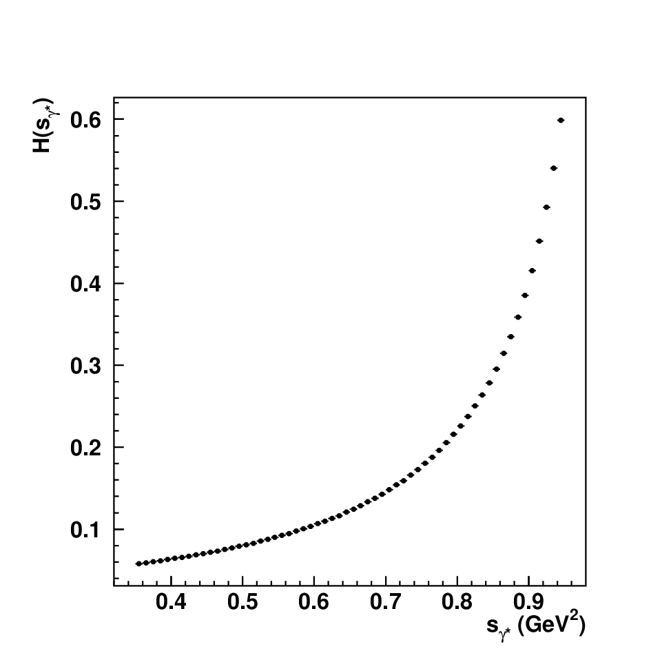
| (97) |
where , the QED kernel, is a monotonic function that varies approximately as , with the squared center-of-mass collision energy, see Fig. 48, left. This amplifies the importance of the cross-section measurements at low energy. Approximately two-thirds of the integral is contributed by the process for GeV, i.e., in the vicinity of . Before the arrival of the KLOE results we discuss below, calculations of from world data (dominated at low energies by the CMD-2 measurement of [13]) led to a value of lower [130] than the final value reported by E821.
10.2 Measurement of and at KLOE
DAΦNE is highly optimized for running at and no large variation of are accessible. However, initial state radiation, ISR, via the process naturally provides access to hadronic states of lower mass. The cross section over the entire interval from threshold to is related to the distribution of for events,
| (98) |
where , the “radiator function,” describes the ISR spectrum. Note the subscript ISR on the differential cross section. This is very important because the contribution from final state photon emission, FSR is of the same order as that from the ISR process unless one imposes special fiducial volume cuts to suppress it.

On the other hand, as is depicted in fig. 49 one must remember eventually to include FSR in the final evaluation of . To correctly calculate and estimate the effects of FSR, an accurate simulation of the is critical. The radiator function used by KLOE to obtain is provided by the Phokhara code [131] by setting the pion form factor , see Fig. 48, right. The Phokhara event generator has been continuously improved by inclusion of next-to-leading-order ISR (two initial-state photons), leading-order FSR and ISR-FSR [132].
Furthermore, has to be corrected for the running of the fine structure constant [133] (vacuum polarization) and for shifting from to the virtual photon mass, for those events with both an initial and a final state radiated photon. The Phokhara version of Ref. [134] contains also these contributions and it is used for the evaluation of the acceptance correction and for all reconstruction efficiencies.
10.2.1 Extraction of and pion form factor
The differential cross section of as a function of is obtained by subtracting, bin by bin, the background events from the number of observed events , correcting for the selection efficiency, , and finally dividing by the total luminosity obtained as described in sect. 3.3:
| (99) |
where our mass resolution allows us to have bins of width .
The background content is found by fitting spectra of selected data sample with a superposition of Monte Carlo distributions describing the signal and background sources. The only free parameters of such fits are the relative weights of signal and backgrounds in data, computed as a function of .
The ”bare” cross section which is obtained after applying the corrections written in eq. 98, inclusive of FSR, is used to determine :
| (100) |
where the lower and upper bounds of the spectrum depend on specific measurement configurations.
The measured is related to the pion form factor via the relation , where is the center-of-mass energy squared, is the pion mass and is the pion velocity in the center-of-mass frame. Since is measured by many experiments, it is customarily used for spectra comparisons.
Two different selection regions are used: the first one is named ”Small angle selection” (SA) since photons are required to be within a cone of around the beam line (narrow cones in fig. 50, left), the second one is called ”Large angle selection” (LA) since there should be at least one photon at a polar angle of (large central cones in fig. 50, left). In both cases the two charged pion tracks should have .


10.2.2 Small angle selection and data analysis
At small photon polar angle , ISR events are vastly more abundant than FSR events. Requiring angular separation between the pions and the photon further suppresses FSR [135]. Thus, the first KLOE measurement [9] was performed using this event selection criterion. Since ISR-photons are mostly collinear with the beam line, a high statistics for the ISR signal events remains. On the other hand, a highly energetic photon emitted at small angle forces the pions also to be at small angles (and thus outside the selection cuts), resulting in a kinematical suppression of events with .
In this analysis the photon is not explicitly detected. Its direction is reconstructed from the tracks’ momenta by closing kinematics: . The separation between pion and photon selection regions greatly reduces the contamination from the resonant process , in which the mimics the missing momentum of the photon(s) and from the final state radiation process .
Discrimination of from events is done via particle identification based on the time of flight, on the shape and the energy of the clusters associated to the tracks. In particular, electrons deposit most of their energy in the first planes of the calorimeter while minimum ionizing muons and pions release uniformly the same energy in each plane. Events with at least one of the two tracks not identified as electron are selected. This criterion results in a rejection power of 97% for events, while retaining a selection efficiency of for events (see fig. 51, left).
Contaminations from the processes and are rejected by cuts on the track mass variable, , defined by the four-momentum conservation, assuming a final state consisting of two particles with the same mass and one photon, and on the missing mass, , defined assuming the process to be .


KLOE first published in 2005 results obtained with 141 pb-1 collected in 2001 [9], which we will refer to as KLOE05 in the following. The statistical errors ranged from 2% at the lower limit in to 0.5% at the peak. The experimental systematic uncertainties were mostly flat in and amounted to 0.9%. The luminosity was estimated using large-angle Bhabha scattering and contributed an additional, dominantly theoretical uncertainty of 0.6%. The cross section was obtained via eq. 98. The contribution to the systematic uncertainty on from FSR was 0.3%, and the theory accuracy of was 0.5%. Finally, for the evaluation of , it was necessary to remove the effects of vacuum polarization in the photon propagator for the process itself by correcting for the running of . This contributes 0.2% to the systematic uncertainty. Thus from KLOE05 analysis we obtained for the contribution to in the energy interval GeV2:
| (101) |
Inclusion of the KLOE05 data together with the CMD-2 data in the evaluation of increased the discrepancy between the calculated and measured values of to () [136]. Furthermore, the precise KLOE spectrum exhibited a pronounced deviation from those derived from lepton’s spectral functions that led to the later being excluded in compilations [136].
KLOE in 2008 completed the analysis of 241 pb-1 data taken in 2002, which we will refer to as KLOE08 in the following. These data benefit from cleaner and more stable running conditions of DAΦNE resulting in less machine background. In particular the following changes are applied with respect to the data taken in 2001: i) an additional trigger level was implemented at the end of 2001 to eliminate a 30% loss due to pions penetrating up to the outer calorimeter plane and being misidentified as cosmic rays events; ii) the offline background filter, which contributed the largest experimental systematic uncertainty (0.6%) to the published work [9], has been improved and includes now a downscale algorithm providing an unbiased control sample. This greatly facilitates the evaluation of the filter efficiency which increased from 95% to 98.5%, with negligible systematic uncertainty; iii) in addition, the knowledge of the detector response and of the KLOE simulation program has been improved. Thus the relative systematic errors on the extraction of in the mass range [0.35,0.95] GeV2 decreased from 1.3% for the 2001 to 0.9% for 2002 data. Finally, we want to stress that the dominant term contributing to the systematic error in KLOE08 analysis is given by the 0.5% uncertainty quoted by the authors of Phokhara [134]. The KLOE08 results are shown in fig. 52. On the left the number of events per 0.01 GeV2 are shown. The differential cross section is shown in the right.


Finally, while performing the 2008 analysis we revisited the published 2001 data analysis, named KLOE05 updated, and we found a bias in the evaluation of the trigger correction that affects mostly the low region. Correcting for this effect and normalizing to the new Bhabha cross section we updated the published spectrum to compare with KLOE08. Fig. 53 , left shows the pion form factor evaluated from these two sets of data. Comparison among values in units of evaluated with the KLOE small angle selection analyses:
KLOE05: ;
KLOE05 Updated: ;
KLOE08: .
We see that in terms of the net shift of the updated value is about one standard deviation below the KLOE05 one and it is also in excellent agreement with the KLOE08 analysis.
Finally, we make a comparison of the most recent evaluations released by the CMD-2 [137] and SND [138] experiments with the KLOE08 [139], in the mass range MeV.
CMD-2: ;
SND: ;
KLOE08: ;
The CMD-2 and SND dispersion integrals are performed with the trapezoid rule, the KLOE value is done extrapolating our bins to match the [630,958] MeV mass range, and summing directly the bin contents of the differential spectrum, weighed for the kernel function.
The CMD-2 and SND values agree with the KLOE08 result within one standard deviation. Thus, inclusion of the latest KLOE results in the world average definitely established without a doubt the discrepancy between the measured and calculated values of , leading to hopes that there is a glimpse of which direction we should search for new physics.


10.2.3 Large angle selection and data analysis
The contribution to from in the interval in between threshold and 0.35 GeV2 is approximately . To explore the low-mass part of the spectrum, KLOE selects events requiring a photon in the calorimeter with energy greater than 50 MeV and . With the photon explicitly detected, about 40% of the background from events is rejected by kinematic closure. A further variable, the 3-dimensional angle between the missing momentum and the photon, which is peaked at 0 degrees for signal events, removes most of the remaining background.
There are however two sources of irreducible background : FSR and . FSR here is a very complicated problem: for ISR and FSR events contribute nearly equally to the spectrum in the tails of the , and the accuracy of the generator used to obtain FSR corrections is critical.
As discussed by Binner et al. in Ref. [135], the ISR-FSR interference results in a measurable charge asymmetry, as well as a distortion in the mass spectrum. The measured charge asymmetry can be used as a useful gauge of the accuracy of the simulation. KLOE has performed comparisons of this type in the analysis of as discussed in the previous section on scalar mesons [139].


We have made a measurement of with photon emitted at large angle using the data collected in 2002. Since it is an independent event selection scheme, by comparing this result with the small angle analysis, we can also test the present models of FSR contributions. Fig. 54 shows both spectra; note that the threshold is reachable with the large angle selection. To make a quantitative comparison, at present we are limited by the unknown interference between the FSR process and the resonant decays as mentioned before. Therefore we limit the comparison to the range where resonance contributions are negligible, that is, to [0.5,0.85] GeV2 where from the ”small angle selection” we obtain and for the ”large angle selection”, , in excellent agreement.
The main source of systematic uncertainty in the large angle selection is the background subtraction.
10.2.4 Pion form factor from
We can also obtain the pion form factor directly from measuring the ratio, R, bin-by-bin of the observed pion and muon (radiative) cross sections. In the absence of photons from final state radiation, one finds [140]
| (102) |
where is the muon mass, and , are the muon and pion velocities in the center-of-mass frame.
The unavoidable presence of photons from final state emission of both the pions and the muons in the data leads to a deviation from the “ideal” eq. 102 which requires treatment of final state radiation (FSR) with care. The advantage of this method is that one does not need an absolute luminosity measurement, thus providing a totally independent measurement of the pion form factor from those obtained using small or large angle selections.
The experimental challenge of measuring the pion form factor using the ratio is the overwhelming cross section over cross section at low momentum, see fig. 55, left. Furthermore, there is an overlap region between the events and events which makes precision event counting/separation a delicate operation. fig. 55, right, shows the separation between and events, achieved selecting different regions around the missing mass peaks. The residual contamination of events are seen at high values.


We are developing additional tools for separation and the results from extracting spectra from using the ratio is extremely promising [141]. We are confident of obtaining from yet another independent method by the end of 2008.
11 Conclusions and outlook
The contributions by KLOE to particle physics during the years 2002-2008 are of great importance. The study of the decays of the kaons have demonstrated unitarity of the CKM matrix with accuracy better than one per mil and universality of the couplings between leptons and quarks. New mass and lifetime values have been obtained. Studies of the meson have reached new levels of precision. KLOE has made the most accurate measurement of the hadronic cross section pertaining to the calculation of the muon anomaly, and has made the most detailed studies on the nature of light scalar mesons.
A summary of all the masses, lifetimes, widths and branching ratios measured by KLOE to date is shown in table 14. Results of tests on conservation of discrete symmetries, as well as on the unitarity of the CKM matrix are shown in table 15.
| Masses (MeV) | ||
| 497.583 0.021 | ||
| 547.874 0.032 | ||
| Lifetimes (ns) | ||
| 50.84 0.23 | ||
| 12.347 0.030 | ||
| Widths (keV) | ||
| 1.32 0.06 | ||
| Branching Ratios | ||
| decays | (6.20 0.27)10-5 | |
| (1.07 0.07) 10-4 | ||
| (7.01 0.24)10-5 | ||
| (4.4 0.6) 10-5 | ||
| 1.8 10-8 at 90 C.L. | ||
| decays | 0.4008 0.0015 | |
| 0.2699 0.0014 | ||
| 0.1996 0.0020 | ||
| 0.1261 0.0011 | ||
| (1.963 0.21)10-3 | ||
| (5.569 0.077)10-4 | ||
| decays | 0.60196 0.00051 | |
| 0.30687 0.00051 | ||
| (7.05 0.09)10-4 | ||
| (2.26 0.13)10-6 | ||
| 1.210-7 at 90 C.L. | ||
| 9.310-9 at 90 C.L. | ||
| decays | 0.6366 0.0017 | |
| 0.2067 0.0012 | ||
| 0.04972 0.00053 | ||
| 0.03237 0.00039 | ||
| 0.01763 0.00034 | ||
| decays | (2.4 0.4) 10-4 | |
| (8.4 3.0)10-5 | ||
| decays | 0.9024 0.0018 | |
| 0.0809 0.0014 | ||
| C symmetry | ||
| 1.6 10-5 | ||
| A | (0.09) 10-2 | |
| A | (-0.05 0.11) 10-2 | |
| A | (0.08) 10-2 | |
| CP symmetry | ||
| (from BR() | (2.216 0.013) )10-3 | |
| (from Bell-Steinberger relation) | (159.6 1.3)10-5 | |
| 1.3 10-5 | ||
| CPT symmetry | ||
| (1.004 0.004) | ||
| (1.5 1.1) MeV | ||
| (1.8 2.1) MeV | ||
| (from Bell-Steinberger relation) | (0.4 2.1)10-5 | |
| (-0.52.5) 10-3 | ||
| with CP symmetry | (1.22.5) 10-3 | |
| Lepton universality | ||
| (from for and ) | 1.000 0.008 | |
| CKM matrix unitarity | ||
| 0.21570.0006 | ||
| 0.2766 0.0009 | ||
| ( from [87]) | ||
It is interesting to note that over half of the results noted above are based on analysis of one fifth of the total KLOE data sample. Several of the measurements have reached the state where additional statistics will not improve accuracy due to theoretical or intermediate state uncertainties as described in the specific sections. There are measurements that could profit with respect to statistical and systematic errors continuing the studies of the entire body of data. Furthermore, several new measurements are only possible using the whole data set whose analysis is expected to be completed in the coming couple of years. These are discussed in the following three subsections. In the fourth subsection we describe a future project KLOE-2 that entails minor upgrade of KLOE in order to complete the original physics program proposed in 1992 but had been stymied by DAΦNE’s limited luminosity. Thus it is clear that we have our hands full for the foreseable future!
11.1 Kaon sector
- 1.
Studies on rare kaon decays can benefit of the use of the entire KLOE statistics. The accuracy in the determination of the branching ratio of events and of the related charge asymmetry will scale with statistics with respect to those shown in sect. 5.4.2, thus reaching 0.5 (fractional) and 510-3 respectively.
- 2.
We have observed the decay channel and will aim at reaching a precision better than 2 on its BR.
- 3.
We plan to improve our limit on decays (see sect. 5.4.4). Preliminary studies have shown that, by slightly modifying the analysis cuts, one can improve on background rejection, while leaving the signal efficiency almost unaffected. This means that we can hope to set the limit on the corresponding BR at the level of 210-8.
- 4.
Moreover, we can search for events, which proceed mainly via a CP-conserving, I = 3/2 transition. A preliminary, but rather detailed, analysis shows that KLOE should be able to measure the corresponding branching ratio with a 60 precision, comparable to the precision with which this BR has been measured by three experiments.
- 5.
The CP violating events can be measured with a 0.5% accuracy, thus setting at the few per mil level the precision on which KLOE can reach.
- 6.
The study of the main decay channels, will allow us to improve our accuracy in the measurement of the lifetime by a factor of 2. We can also improve the precision in the measurement of the scalar form factor for semileptonic decays by the same amount.
- 7.
The form factor slopes for can be measured as well, using about 5.9 and about 2.5 decays from the entire data sample. It is important to note that in the scalar form factor measurement from there is no ambiguity.
- 8.
The accuracy on the lifetime can be improved by a factor 1.5. As discussed in sect. 6, these are key ingredients for the determination of the CKM matrix element .
- 9.
Semi-rare charged kaon decay channels can also be studied. In particular, we are planning to measure the branching ratio of the decay into three charged pions. With the present data sample a few per mil statistical accuracy can be reached. Using the same data set the measurement of the branching ratio of the decay can reach a 10% statistical accuracy. This will allow us to complete the measurement of the main branching ratios.
11.2 Light meson spectroscopy
Many analyses on light meson spectroscopy could be refined in the future. Although the level of accuracy for the measurements on the scalar sector has already reached its limit, a combined analysis of different final states, such as /, will give more insight into the structure of light scalar mesons.
On the other hand, the pseudoscalar mesons could benefit from the larger statistics of the whole KLOE data sample.
- 1.
In particular, we can complete the study of the main decay channels by measuring the BR’s of , with a statistical precision of few per mil.
- 2.
Moreover, the knowledge on numerous rare decay channels can be improved. Apart from lowering the limits on C (P,CP) violating decays (), we could reach a statistical precision of 3.5% on the BR() and measure for the first time the asymmetry between the and decay planes. The knowledge of the systematics for the latter decay could reach a few % accuracy by relying on large data/MC control samples. An observation at the level of 100 events is expected for the double Dalitz decay .
- 3.
Finally, the BR() will reach a 1.5% statistical accuracy. Improvements of the analysis based on a new clustering scheme and on a photon veto at small angle could reduce the related systematics and background contamination, allowing also the measurement of the invariant mass spectra.
- 4.
For the , we have in hand about 450,000 of these mesons, so precise measurements could now be carried out. We plan to do this in three ways:
i. looking at the dynamics by studying the Dalitz plot for the , processes;
ii. measuring ratio of branching fractions for some of the main decay channels, such as , , , thus improving their BR accuracy;
iii. searching for never heretofore observed decay channels, whose upper limits are at the % level (, )
11.3 Pion form factor at about 1 GeV
In early 2006, KLOE also collected 200 pb-1 of data at MeV, at which drops to 5% of its peak value. These data by themselves should determine the contribution to normalizing to absolute luminosity, with a statistical error of . This will give us another check on our measurements using the previously mentioned three methods: small angle selection, large angle selection and to ratio.
11.4 KLOE-2
In late 2007 an important accelerator experiment has begun at DAΦNE, with the goal of increasing the machine’s luminosity by a factor of at least three, from the implementation of an innovative interaction scheme [142].
The exciting perspective of collecting much more data within a few years, inspired many KLOE members, together with several new collaborators, to form a new enterprise with the goal of continuing the KLOE physics program with an upgraded detector [143].
This project, dubbed with a certain lack of fantasy KLOE-2, foresees the insertion of new subdetectors in the inner part of KLOE, between the beryllium beam pipe and the internal wall of the drift chamber. An inner tracking chamber, based on the GEM technology is being developed at LNF. Crystal calorimeters will help catching photons emitted at very low polar angles. These detectors will increase acceptance for many physics channels, especially for , and ’ decays. The implementation of a detector to tag interactions is also under study.
KLOE-2 is an ambitious project, which requires a few years of preparation and a longer period of data taking: the goal is to acquire at least 20-30 fb-1 by year 2012.
Appendix A. The KLOE Collaboration: inclusive to 2008
F. Adinolfi j,k,
F. Ambrosino e,f,
A. Antonelli a,
M. Antonelli a,
F. Archilli j,k,
C. Bacci l,m,
M. Barva l,m,
P. Beltrame b,
G. Bencivenni a,
S. Bertolucci a,
C. Bini h,i,
C. Bloise a,
S. Bocchetta l,m,
V. Bocci i,
F. Bossi a,
D. Bowring a,p,
P. Branchini m,
R. Caloi h,i,
P. Campana a,
G. Capon a,
T. Capussela a,
M. Casarsa r,
F. Ceradini l,m,
F. Cervelli s,
S. Chi a,
G. Chiefari e,f,
P. Ciambrone a,
F. Crucianelli h,
S. Conetti p,
E. De Lucia a,
A. De Santis h,i,
P. De Simone a,
G. De Zorzi h,i,
S. Dell’Agnello a,
A. Denig b,
A. Di Domenico h,i,
C. Di Donato f,
B. Di Micco l,m,
S. Di Falco s,
A. Doria f,
M. Dreucci a,
O. Erriquez t,
A. Farilla m,
G. Felici a,
A. Ferrari a,
M. L. Ferrer a,
G. Finocchiaro a,
S. Fiore h,i,
C. Forti a,
P. Franzini h,i,
C. Gatti a,
P. Gauzzi h,i,
S. Giovannella a,
E. Gorini c,d,
E. Graziani m,
M. Incagli s,
W. Kluge b,
V. Kulikov q,
F. Lacava h,i,
G. Lanfranchi a,
J. Lee-Franzini a,n,
D. Leone b,
M. Martemianov q,
M. Martini a,g,
P. Massarotti e,f,
W. Mei a,
S. Meola e,f,
S. Miscetti a,
M. Moulson a,
S. Müller a,
F. Murtas a,
M. Napolitano e,f,
F. Nguyen l,m,
M. Palutan a,
E. Pasqualucci i,
L. Passalacqua a,
A. Passeri m,
V. Patera a,g,
F. Perfetto e,f,
L. Pontecorvo i,
M. Primavera d,
P. Santangelo a,
E. Santovetti j,k,
G. Saracino e,f,
B. Sciascia a,
A. Sciubba a,g,
F. Scuri s,
I. Sfiligoi a,
A. Sibidanov a,
T. Spadaro a,
E. Spiriti m,
M. Tabidze a,u,
M. Testa h,i,
L. Tortora m,
P. Valente i,
B. Valerianib,
G. Venanzoni a,
S. Veneziano i,
A. Ventura d,
S.Ventura h,i,
R. Versaci a,g,
G. Xu a,o.
aLaboratori Nazionali di Frascati dell’INFN, Via E. Fermi 40, I-00044 Frascati, Italy
bInstitut für Experimentelle Kernphysik, Universität Karlsruhe, D-76128 Karlsruhe,Germany
cDipartimento di Fisica dell’Università del Salento, Via Arnesano, I-73100 Lecce, Italy
dINFN Sezione di Lecce, Via Arnesano, I-73100 Lecce, Italy
eDipartimento di Scienze Fisiche dell’Università di Napoli “Federico II”, Via Cintia, I-80126 Napoli, Italy
fINFN Sezione di Napoli, Via Cintia, I-80126 Napoli, Italy
gDipartimento di Energetica dell’Università di Roma “La Sapienza”, P. Aldo Moro 2, I-00185 Roma, Italy
hDipartimento di Fisica dell’Università di Roma “La Sapienza”, P. Aldo Moro 2, I-00185 Roma, Italy
iINFN Sezione di Roma, P. Aldo Moro 2, I-00185 Roma, Italy
jDipartimento di Fisica dell’Università di Roma “Tor Vergata”,
Via della Ricerca Scientifica 1, I-00133 Roma, Italy
kINFN Sezione di Roma Tor Vergata, Via della Ricerca Scientifica 1, I-00133 Roma, Italy
lDipartimento di Fisica dell’Università di Roma “Roma Tre”, Via della Vasca Navale 84, I-00146 Roma, Italy
mINFN Sezione di Roma Tre, Via della Vasca Navale 84, I-00146 Roma, Italy
nPhysics Department, State University of New York at Stony Brook, Stony Brook, NY 11794-3840 USA
oInstitute of High Energy Physics of Academia Sinica, P.O. Box 918 Beijing 100049, P.R. China
pPhysics Department, University of Virginia, Virginia, USA
qInstitute for Theoretical and Experimental Physics, B. Cheremushkinskaya ul. 25 RU-117218 Moscow, Russia
rDipartimento di Fisica dell’Università e Sezione INFN di Trieste, Trieste, Italy
sDipartimento di Fisica dell’Università e Sezione INFN di Pisa, Pisa, Italy
tDipartimento di Fisica dell’Università e Sezione INFN di Bari, Bari, Italy
uHigh Energy Physics Institute, Tbilisi State University, Tbilisi, Georgia
Acknowledgements
We thank the DAΦNE team for their efforts in maintaining low background running conditions and their collaboration during all data-taking. We want to thank our technical staff: G.F.Fortugno for his dedicated work to ensure an efficient operation of the KLOE Computing Center; M.Anelli for his continuous support to the gas system and the safety of the detector; A.Balla, M.Gatta, G.Corradi and G.Papalino for the maintenance of the electronics; M.Santoni, G.Paoluzzi and R.Rosellini for the general support to the detector; C.Piscitelli for his help during major maintenance periods. This work was supported in part by DOE grant DE-FG-02-97ER41027; by EURODAPHNE, contract FMRX-CT98-0169; by the German Federal Ministry of Education and Research (BMBF) contract 06-KA-957; by Graduiertenkolleg ‘H.E. Phys. and Part. Astrophys.’ of Deutsche Forschungsgemeinschaft, Contract No. GK 742; by INTAS, contracts 96-624, 99-37; and by the EU Integrated Infrastructure Initiative HadronPhysics Project under contract number RII3-CT-2004-506078.
References
- [1] Preprint LNF-90/031(R), (1990). http://www.lnf.infn.it/sis/preprint.
- [2] M. Adinolfi et al. (KLOE Collab.), Nucl. Instrum. Meth. A 488 (2002) 51.
- [3] A. Balla et al. (KLOE Collab.), Nucl. Instrum. Meth. A 562 (2006) 141.
- [4] A. Aloisio et al. (KLOE Collab.), Nucl. Instrum. Meth. A 516 (2004) 288.
- [5] M. Adinolfi et al. (KLOE Collab.), Nucl. Instrum. Meth. A 482 (2002) 364.
- [6] M. Adinolfi et al. (KLOE Collab.), Nucl. Instrum. Meth. A 483 (2002) 649.
- [7] M. Adinolfi et al. (KLOE Collab.), Nucl. Instrum. Meth. A 492 (2002) 134.
- [8] F. Ambrosino et al. (KLOE Collab.), Nucl. Inst. Meth. A 534 (2004) 403.
- [9] A. Aloisio et al. (KLOE Collab.) Phys. Lett. B 606 (2005) 12.
- [10] M. Testa, and the KLOE Collab., arXiv:0805.1969.
- [11] C. M. Carloni Calame et al., Nucl. Phys. B 584 (2000) 459.
- [12] R. R. Akhmetshin et al., Phys. Lett. B466 (1999) 385.
- [13] R. R. Akhmetshin et al., Phys. Lett. B578 (2004) 285.
- [14] A. Aloisio et al. (KLOE Collab.), Phys. Lett. B 538 (2002) 21.
- [15] F. Ambrosino et al. (KLOE Collab.), Phys. Lett. B 535 (2002) 37.
- [16] A. Aloisio et al. (KLOE Collab.), Phys. Lett. B 537 (2002) 21.
- [17] A. Aloisio et al. (KLOE Collab.), Phys. Lett. B 536 (2002) 209.
- [18] A. Aloisio et al. (KLOE Collab.), Phys. Lett. B 541 (2002) 45.
- [19] F. Ambrosino et al. (KLOE Collab.), Eur. Phys. J. C 47 (2006) 589.
- [20] G. Balossini et al., Nucl. Phys. B 758 (2006) 227.
- [21] Particle Data Group, W.-M. Yao., et al., J. Phys. G 33 (2006) 1 and web update for 2008 edition.
- [22] C. Gatti Eur. Phys. J. C 45 (2006) 417.
- [23] M. Greco et al., in The Second DANE Physics Handbook, L. Maiani, N. Paver (Eds) SIS-Pubblicazioni Frascati (1995), 629.
- [24] E. A. Kuraev, V. .S. Fadin, Sov. J. Phys. 41 (1985) 3.
- [25] F. Ambrosino et al. (KLOE Collab.), JHEP 12 (2007) 073.
- [26] F. Ambrosino et al. (KLOE Collab.), Phys. Lett. B 632 (2006) 43.
- [27] F. Ambrosino et al. (KLOE Collab.), Phys. Lett. B 626 (2005) 15.
- [28] F. Ambrosino et al. (KLOE Collab.), JHEP 01 (2008) 073.
- [29] F. Ambrosino et al. (KLOE Collab.), Eur. Phys. J. C 48 (2006) 767.
- [30] V. Cirigliano et al., Eur. Phys. J. C 48 (2004) 369.
- [31] F. Ambrosino et al. (KLOE Collab.), Phys. Lett. B 636 (2006) 173.
- [32] Maiani L., in The Second DANE Physics Handbook, L. Maiani, N. Paver (Eds) SIS-Pubblicazioni Frascati (1995), 3.
- [33] A. Angelopoulos et al., (CPLEAR Collab.), Phys. Lett. B 444 (1998) 52.
- [34] A. Apostolakis et al., (CPLEAR Collab.), Phys. Lett. B 456 (1999) 297.
- [35] G. D’ambrosio, D. Esprin, Phys. Lett. B 175 (1986) 237.
- [36] J. R. Bartley et al., Phys. Lett. B 551 (2003).
- [37] F. Ambrosino et al. (KLOE Collab.), JHEP 05 (2008) 51.
- [38] G. D’Ambrosio et al., in The Second DANE Physics Handbook, L. Maiani, N. Paver (Eds) SIS-Pubblicazioni Frascati (1995), 63.
- [39] F. Ambrosino et al. (KLOE Collab.), Phys. Lett. B 619 (2005) 61.
- [40] A. Lai et al. (NA48 Collab.), Phys. Lett. B 610 (2005) 165.
- [41] G. Ecker and A. Pich, Nucl. Phys. B 366 (1991) 189.
- [42] A. Angelopoulos et al. (CPLEAR Collab.), Phys. Lett. B 413 (1997) 232.
- [43] F. Archilli and the KLOE Collaboration, arXiv:0805.2262 (2008).
- [44] M. Ademollo and R. Gatto, Phys. Rev. Lett. 13 (1964) 264.
- [45] P. Franzini, Kaon Int. Conf. 2007, Opening remarks, PoS(KAON)002 (2007).
- [46] T. Alexopolous et al. (KTeV Collab.), Phys. Rev. D 70 (2004) 092007.
- [47] A. Lai et al. (NA48 Collab.), Phys. Lett. B 606 (2004) 1.
- [48] F. Ambrosino et al. (KLOE Collab.), Phys. Lett. B 636 (2006) 166.
- [49] V. Bernard, M. Oertel, E. Passemar and J. Stern, Phys. Lett. B 638 (2006) 480.
- [50] M. Jamin, A. Pich and J. Portoles, Phys. Lett. B 640 (2006) 176.
- [51] A. Lai et al. (NA48 Collab.), Phys. Lett. B 647 (2007) 341.
- [52] O. P. Yushchenko et al., Phys. Lett. B 581 (2004) 31.
- [53] C. G. Callan, S. Treiman, Phys. Rev. Lett. 16 (1966) 153.
- [54] J. Gasser, H. Leutwyler, Nucl. Phys. B 250 (1985) 93.
- [55] M. Jamin, J. A. Oller and A. Pich, Phys. Rev. D 74 (2006) 074009.
- [56] F. Ambrosino et al. (KLOE Collab.), JHEP 12 (2007) 105.
- [57] E. Follana, et al. (HPQCD/UKQCD Collab.) arXiv:0706.1726, 2007.
- [58] P.A. Boyle, et al. (RBC/UKQCD Collab.), arXiv:0710.5136, 2007.
- [59] J. Gasser, B. Kubis, N. Paver, M. Verbeni, Eur. Phys. J. C 40, (2005) 205.
- [60] F. Ambrosino et al. (KLOE Collab.), Eur. Phys. J. C 55 (2008) 539.
- [61] J. H. Christenson, J. W. Cronin, V. L. Fitch, R. Turlay, Phys. Rev. Lett. 13 (1964), 138.
- [62] N. Cabibbo, Phys. Rev. Lett. 10 (1963) 531.
- [63] M. Kobayashi, T. Maskawa, Prog. Theor. Phys. 652 (1973) 49.
- [64] F. Ambrosino et al. (KLOE Collab.), Phys. Lett. B 638 (2006) 140.
- [65] E. Ramberg et al., Phys. Rev. Lett. 70 (1993) 2525.
- [66] M. Bona et al. (UTfit Collab.), JHEP 507 (2005) 28.
- [67] G. D’Ambrosio et al., in The Second DANE Physics Handbook, L. Maiani, N. Paver (Eds) SIS-Pubblicazioni Frascati (1995), 205.
- [68] F. Ambrosino et al. (KLOE Collab.), Phys. Lett. B 566 (2003) 61.
- [69] F. Ambrosino et al. (KLOE Collab.), Phys. Lett. B 632 (2006) 76.
- [70] F. Ambrosino et al. (KLOE Collab.), Phys. Lett. B 666 (2006) 305.
- [71] F. Ambrosino et al. (KLOE Collab.), JHEP 02 (2008) 098.
- [72] A. Aloisio et al. (KLOE Collab.), Phys. Lett. B 597 (2004) 139.
- [73] F. Ambrosino et al. (KLOE Collab.), PoS(KAON)050 (2007).
- [74] A. Masiero, P. Paradisi and R. Petronzio, Phys. Rev. D 74 (2006) 011701.
- [75] S. Eidelman et al., Phys. Lett. B 592 (2004) 1. The average value is evaluated using: D. Pandoulas et al., Phys. Rev. D2 (1970) 1205; A. de Marco et al., Phys. Rev. 140B (1965) 1430; A. Callahan et al., Phys. Rev. 136B (1964) 1463; F.S. Shaklee et al., Phys. Rev. 136B (1964) 1423.
- [76] C. Klopfenstein et al. (CUSB Collab.), Phys. Lett. B 130 (1983) 444.
- [77] A. Sirlin, Nucl. Phys. B 196 (1982) 83.
- [78] P. Franzini and M. Moulson, Ann. Rev. Nucl. Part. Sci. 56 (2006), 207.
- [79] V. Cirigliano et al., Eur. Phys. J. C 23 (2002) 121.
- [80] S. Descotes-Genon and B. Moussallam, Eur. Phys. J. C 42, 403 (2005).
- [81] V. Cirigliano, Kaon Int. Conf. 2007, Precision tests of the Standard Model with , PoS(KAON)007 (2007).
- [82] F. Ambrosino et al. (KLOE Collab.), JHEP 04 (2008) 059.
- [83] H. Leutwyler and M. Roos, Z. Physik 25(1984) 91.
- [84] M.J. Ramsey-Musolf, et al. arXiv:0705.0028, 2007.
- [85] W. Marciano, Phys. Rev. Lett. 93 (2004) 231803.
- [86] G. Isidori and P. Paradisi, Phys. Lett. B 639 (2006) 499.
- [87] I.S. Towner and J.C. Hardy, arXiv:0710.3181, 2007.
- [88] K. Ikado, et al. (Belle Collab.), Phys. Rev. Lett. 97, 251802 (2006); B. Aubert et al. (BaBar Collab.), arXiv:0705.1820, 2007.
- [89] F. Ambrosino et al. (KLOE Collab.), Phys. Lett. B 642 (2006) 315.
- [90] J. Bernabeu, N. Mavromatos, J. Papavassiliou, Phys. Rev. Lett. 92, 131601 (2004).
- [91] J. Bernabeu et al., Nucl. Phys. B 744, 180 (2006).
- [92] G. Lüders, Annals Phys. 2 (1957) 1, [Annals Phys. 281 (2000) 1004].
- [93] See e.g. V.A. Kostelecky and R. Lehnert, Phys. Rev. D 63 (2001) 065008; N. E. Mavromatos, AIP Conf. Proc. 796 (2005) 13.
- [94] J.S. Bell and J. Steinberger, in Proc. Oxford Int. Conf. on Elementary Particles, Walsh T. R. et al. (Eds) Rutherford Chilton (1966) 200.
- [95] F. Ambrosino et al. (KLOE Collab.), JHEP 12 (2006) 011.
- [96] J. N. Matthews et al., Phys. Rev. Lett. 75 (1995) 2806.
- [97] A. Angelopoulos et al. (CPLEAR Collab.), Phys. Rept. 374 (2003) 165.
- [98] V. A. Kostelecky, Phys. Rev. Lett. 80, 1818 (1998); ibid 61, 016002 (1999); ibid 64, 076001 (2001).
- [99] F. Ambrosino et al. (KLOE Collab.), Phys. Lett. B 606 (2005) 276.
- [100] A. Aloisio et al. (KLOE Collab.), Phys. Lett. B 591 (2004) 49.
- [101] A. Lai et al. (NA48 Collab.), Phys. Lett. B 533 (2002) 196.
- [102] D. H. Miller et al., Phys. Rev. Lett. 99 (2007) 122002.
- [103] M. Abdel-Bary et al., Phys. Lett. B 619 (2005) 281.
- [104] F. Ambrosino et al. (KLOE Collab.), JHEP 05 (2008) 006.
- [105] J. Bijnens and J. Gasser, Physica Scripta T99, 34 (2002).
- [106] B. Borasoy, R. Nissler, hep-ph/0510384 v2.
- [107] G. D’Ambrosio, G. Isidori, Int. J. Mod. Phys. A13, 1 (1998).
- [108] F. Ambrosino, et al. (KLOE Collab.) hep-ex/0707.4137.
- [109] Eta Physics Handbook, J. Bijnens J, G. Galt, B.M.K. Nefkens, eds., Proc. Workshop Eta Phys., Uppsala, 2001. Phys. Scripta T99 (2002).
- [110] D. N. Gao, Mod. Phys. Lett. A 17 (2002) 1583.
- [111] R. Versaci et al. (KLOE Collab.), Proc. XII Int. Conf. on Hadron Spectroscopy, Frascati Physics Series, Vol. XLVI (2007).
- [112] Th. Feldmann, Int. J. Mod. Phys. A 159 (2000) 15.
- [113] A. Bramon, R. Escribano and M.D. Scadron Eur. Phys. J. C 7 (1999) 271.
- [114] A. Bramon, R. Escribano and M.D. Scadron Phys. Lett. B 503 (2001) 271.
- [115] F. Ambrosino et al. (KLOE Collab.), Phys. Lett. B 238 (2007) 52.
- [116] P. J. Franzini, W. Kim and J. Lee-Franzini, Phys. Lett. B 287 (1992) 259.
- [117] N.N. Achasov, V.N. Ivanchenko Nucl. Phys. B 315 (1989) 465.
- [118] G. Isidori, et al., JHEP 05 (2006) 049.
- [119] F. Ambrosino et al. (KLOE Collab.), Eur. Phys. J. C 49 (2007) 473.
- [120] N. N. Achasov, A.V. Kiselev, Phys. Rev. D 73 (2006) 054029.
- [121] F. Ambrosino et al. (KLOE Collab.), Phys. Lett. B 634 (2006) 148.
- [122] H. Czyż, A. Grzelińska and J. H. Kühn, Phys. Lett. B 611 (2005) 116.
- [123] G. Pancheri, O. Shekhovtsova and G. Venanzoni, Phys. Lett. B 642 (2006) 342.
- [124] F. Ambrosino et al. (KLOE Collab.), arXiv:0707.4148.
- [125] F. Ambrosino et al. (KLOE Collab.), Phys. Lett. B 608 (2005) 199.
- [126] A. London et al., Phys. Rev. 143 1034 (1966); G. Cosme et al., Phys. Lett. B 48 155 (1974); G. Parrour et al., Phys. Lett. B 63 357 (1976).
- [127] A. Aloisio et al. (KLOE Collab.), Phys. Lett. B 561 (2003) 55.
- [128] F. Ambrosino et al. (KLOE Collab.), Phys. Lett. B 669 (2008) 223.
- [129] G. W. Bennett et al. (Muon Collab.), Phys. Rev. Lett. 92 (2004) 161802; idem Phys. Rev. D 73 (2006) 072003.
- [130] M. Davier, W. J. Marciano Annu. Rev. Nucl. Part. Sci. 54:115 (2004).
- [131] G. Rodrigo, H. Czyż, J. H. Kühn and M. Szopa, Eur. Phys. J. C 24 (2002) 71.
- [132] H. Czyż, A. Grzelińska, J. H. Kühn, G. Rodrigo Eur. Phys. J. C 33:333 (2004).
- [133] F. Jegerlehner, Nucl. Phys. Proc. Suppl. 162 (2006) 22.
- [134] H. Czyż, A. Grzelińska, J. H. Kühn and G. Rodrigo, Eur. Phys. J. C 47 (2006) 617.
- [135] S. Binner, J. H .Kühn, K. Melnikov Phys. Lett. B 459:279 (1999).
- [136] A. Höcker, H. Chen, D. Du, W. Li, C. Lu, eds. Proc. Int. Conf. High Energy Phys. (ICHEP), 32nd, Beijing, 2004, Singapore: World Sci. (2005) 710.
- [137] R.R.Akhmetshin et al. (CMD-2 Collab.), Phys. Lett. B 648 (2007) 28.
- [138] M. N. Achasov et al. (SND Collab.), J. Exp. Theor. Phys. 103 (2006) 380.
- [139] F. Ambrosino et al. (KLOE Collab.), to be published in Phys. Lett. B, arXiv:0809.3950.
- [140] H. Czyż, A. Grzelińska,, J. Kühn, G. Rodrigo, Eur. Phys. J. C 39 (2005), 411.
- [141] F. Ambrosino et al. (KLOE Collab.), arXiv: 0807.1612, Nucl. Phys. Proc. Suppl. (2008).
- [142] D. Alesini et al., LNF-06/33 (IR) (2006).
- [143] http://www.lnf.infn.it/lnfadmin/direzione/KLOE2-Loi.pdf .