Semiclassical Theory for Decay and Fragmentation Processes
in Chaotic Quantum Systems

Martha Gutiérrez Affiliation: Institut für Theoretische Physik, Universität Regensburg, D-93040 Regensburg, Germany Daniel Waltner Affiliation: Institut für Theoretische Physik, Universität Regensburg, D-93040 Regensburg, Germany Jack Kuipers Affiliation: Institut für Theoretische Physik, Universität Regensburg, D-93040 Regensburg, Germany Klaus Richter Affiliation: Institut für Theoretische Physik, Universität Regensburg, D-93040 Regensburg, Germany

August 24, 2026

Abstract

We consider quantum decay and photofragmentation processes in open chaotic systems in the semiclassical limit. We devise a semiclassical approach which allows us to consistently calculate quantum corrections to the classical decay to high order in an expansion in the inverse Heisenberg time. We present results for systems with and without time reversal symmetry and also for the symplectic case, as well as extending recent results to non-localized initial states. We further analyze related photodissociation and photoionization phenomena and semiclassically compute cross-section correlations, including their Ehrenfest time dependence.

pacs

03.65.Sq,05.45.Mt, 05.45.Pq

I I. Introduction

Physical phenomena involving decay processes have been addressed in many physical contexts. They play a central role in the study of excitation relaxation in semiconductor quantum dots and wires [1, 2], photoionization via highly excited atomic [3] or molecular [4] Rydberg states, photodissociation of molecules [5], atoms in optically generated lattices and cavities [6], and optical micro-cavities [7], to name a few examples.

For an open chaotic system it is well known that the classical probability of finding a particle inside the system at a certain time, the classical survival probability, decays exponentially in time, $\rho^{\rm cl}(t)=e^{-t/\tau_{d}}$ , where $\tau_{d}$ is the classical life or dwell time. Numerical calculations [8], however, revealed that the quantum survival probability deviates from the classical one at times comparable to $t^{*}\approx\sqrt{\tau_{d}t_{H}}$ , where $t_{H}=2\pi\hbar/\Delta$ is the Heisenberg time, and $\Delta$ is the mean level spacing. Theoretical calculations invoking supersymmetry techniques [9, 10] confirmed these findings. There it could be shown that in the random matrix theory (RMT) limit, the quantum decay $\rho(t)$ takes the form of a universal function, which only depends on the general symmetries of the system, the classical life time and the Heisenberg time. The first successful semiclassical approach to derive the RMT predictions for quantum graphs was performed in Ref. [11], reproducing the first order RMT quantum corrections for networks with and without time-reversal symmetry.

Recently, we have developed a semiclassical approach for calculating the decay of an initially localized wave function inside an arbitrary chaotic system [12]. The semiclassical framework used there involves correlated trajectories which have been shown to be a powerful tool and the key to link classical hyperbolic dynamics with universal quantum properties [13]. These semiclassical techniques have been recently extended and widely applied in the context of level statistics [14, 15, 16], where multiple sums over periodic orbits have to be evaluated, as well as in the field of ballistic quantum transport involving Landauer-Büttiker formulas [17, 18, 19, 20, 21, 22, 23], where trajectories start and end at the openings where the chaotic conductor is attached to leads. In Ref. [12] a unitarity problem was encountered when using these semiclassical techniques to evaluate the contribution of pairs of interfering trajectories starting and ending inside the system. Therefore a new kind of diagram was considered, which is crucial for ensuring unitarity in problems involving open trajectories connecting two arbitrary points in the bulk. A similar type of trajectory appears in the semiclassical description of transport if the coupling between the chaotic conductor and the leads is not perfect, as shown in Ref. [24].

In this article we generalize the approach presented in Ref. [12] for localized initial wave functions to non-localized wave functions. We outline how to systematically obtain higher order (in $t/t^{\ast}$ ) quantum corrections to the classical decay and present terms up to the 7th order and 8th order, for systems with and without time reversal symmetry, respectively. We further calculate the survival probability for systems with spin-orbit interaction, corresponding to the symplectic RMT ensemble.

Closely related to quantum decay are problems of atomic photoionization or molecular photodissociation where the fragmentation mechanism involves photoexcitation to an intermediate excited resonant state (with corresponding complex classical dynamics) which then subsequently decays by sending out a particle, i.e. an electron, atom or an ion. In the semiclassical limit, spectral correlation functions for the related photoionization and photodissociation cross-sections can be expressed through the spectral form factor and the survival probability. Earlier semiclassical treatments [25, 26] of photo cross-sections were always limited through the diagonal approximation used which was relaxed in this context only very recently [12]. Here we will present a detailed semiclassical treatment of the brief account given in [12] and extent the results by including Ehrenfest time effects for cross-section correlations and by computing higher order contributions.

This article is organized as follows: in Secs. II and III we present the semiclassical approach to the quantum survival probability, generalized to non-localized wave functions, by including a time average. In Sec. IV this approach is further extended to derive higher order corrections for systems with and without time reversal symmetry as well as for the case of spin-orbit interaction which follows the universal RMT prediction for the symplectic case. In Sec. V we analyze fluctuations of the survival probability through its variance. In Sects. VI and VII we give a detailed semiclassical analysis of the statistics of photofragmentation, including higher order corrections and the Ehrenfest time dependence of the leading quantum contributions. We conclude with an outlook in Sec. VIII.

II II. Semiclassical approach to the survival probability

The quantum mechanical survival probability as a measure of the decay is defined as

\rho\left(t\right)=\int_{A}d{\bf r}\,\psi({\bf r},t)\psi^{*}({\bf r},t)\,,

(1)

where $\psi({\bf r},t)$ is a wave function and $A$ the volume of the system we are considering. For a closed system $\rho(t)=1$ , while for an open system this no longer holds and $\rho(t)$ decays in time. Expressing $\psi({\bf r},t)$ in terms of the propagator $K({\bf r},{\bf r^{\prime}},t)$ ,

\psi({\bf r},t)=\int_{A}d{\bf r^{\prime}}K({\bf r},{\bf r^{\prime}},t)\psi_{0}({\bf r^{\prime}})\,,

(2)

we have

\rho\left(t\right)=\int_{A}d{\bf r}d{\bf r^{\prime}}d{\bf r^{\prime\prime}}K({\bf r},{\bf r^{\prime}},t)K^{*}({\bf r},{\bf r^{\prime\prime}},t)\psi_{0}({\bf r^{\prime}})\psi_{0}^{*}({\bf r^{\prime\prime}})\,,

(3)

where $\psi_{0}({\bf r})$ is the initial wave function at $t=0$ .

In order to calculate the semiclassical expression for $\rho\left(t\right)$ , we replace the exact quantum propagator $K({\bf r},{\bf r^{\prime}},t)$ with the semiclassical Van Vleck propagator [27],

K^{\rm sc}\left(\mathbf{r},\mathbf{r^{\prime}},t\right)=\frac{1}{(2\pi i\hbar)^{f/2}}\sum_{\tilde{\gamma}\left(\mathbf{r^{\prime}}\to\mathbf{r},t\right)}D_{\tilde{\gamma}}{\rm e}^{\frac{i}{\hbar}S_{\tilde{\gamma}}(\mathbf{r},\mathbf{r^{\prime}},t)}\,.

(4)

Here $f$ is the dimension of the system (in the following we will consider $f=2$ ), $S_{\tilde{\gamma}}({\bf r},{\bf r^{\prime}},t)=\int_{0}^{t}dt^{\prime}L_{\tilde{\gamma}}[\dot{\mathbf{r}}_{\tilde{\gamma}},{\mathbf{r}}_{\tilde{\gamma}},t^{\prime}]$ is the classical Hamilton’s principal function (with $L_{\tilde{\gamma}}$ the Lagrangian) along the path $\tilde{\gamma}$ connecting ${\bf r}^{\prime}$ and ${\bf r}$ in a time $t$ , and $D_{\tilde{\gamma}}=\left|{\rm det}\left(-\frac{\partial^{2}S_{\tilde{\gamma}}({\bf r},{\bf r^{\prime}},t)}{\partial{\bf r}\partial{\bf r^{\prime}}}\right)\right|^{1/2}{\rm e}^{-i\frac{\pi}{2}\mu_{\tilde{\gamma}}}$ is the Van Vleck determinant including the Morse index $\mu_{\tilde{\gamma}}$ .

The semiclassical survival probability is then given by

	$\displaystyle\rho^{\rm sc}(t)$	$\displaystyle=$	$\displaystyle\frac{1}{(2\pi\hbar)^{2}}\int_{A}d{\mathbf{r}}d{\mathbf{r}}^{\prime}d{\mathbf{r}}\psi_{0}({\mathbf{r}}^{\prime})\psi_{0}^{*}({\mathbf{r}}^{\prime\prime})\times$		(5)
			$\displaystyle\times\sum_{\tilde{\gamma}\left(\mathbf{r}^{\prime}\to\mathbf{r},t\right)\atop\tilde{\gamma}^{\prime}\left(\mathbf{r}^{\prime\prime}\to\mathbf{r},t\right)}D_{\tilde{\gamma}}D_{\tilde{\gamma}^{\prime}}^{*}{\rm e}^{\frac{i}{\hbar}(S_{\tilde{\gamma}}-S_{\tilde{\gamma}^{\prime}})}.$		(5)

In the following, we introduce a local time average in the survival probability which enables us to neglect highly oscillating terms in the above double sum. We define

\bar{\rho}(t)\equiv\langle\rho^{\rm sc}(t)\rangle_{\Delta t}\equiv\frac{1}{\Delta t}\int_{t-\Delta t/2}^{t+\Delta t/2}\rho^{\rm sc}(t^{\prime})dt^{\prime}

(6)

with $\Delta t\ll t$ . We will later see that for a localized initial wave packet $\bar{\rho}(t)\approx\rho(t)$ in the semiclassical limit, recalling the result of Ref. [12].

The phase difference in the double sum in Eq. (5) rapidly oscillates unless the two related trajectories are correlated. Therefore most of the contributions will disappear due to the time average. The contributions that prevail the average are from pairs of correlated trajectories with action differences of the order of $\hbar$ , which implies that the trajectories $\tilde{\gamma}$ and $\tilde{\gamma}^{\prime}$ should be ‘similar’. This puts a restriction on the initial points of the two trajectories, i.e. they should be almost the same. We can then expand trajectories $\tilde{\gamma}$ (or $\tilde{\gamma}^{\prime}$ ) going from $\mathbf{r}^{\prime}$ (or $\mathbf{r}^{\prime\prime}$ ) to $\mathbf{r}$ in a time t around trajectories $\gamma$ (or $\gamma^{\prime}$ ) going from $\mathbf{r}_{0}=(\mathbf{r}^{\prime}+\mathbf{r}^{\prime\prime})/2$ to $\mathbf{r}$ in a time $t$ . This expansion amounts to approximating the classical prefactors $D_{\tilde{\gamma}}\left(\mathbf{r},\mathbf{r}^{\prime},t\right)\approx D_{\gamma}\left(\mathbf{r},\mathbf{r}_{0},t\right)$ and $D_{\tilde{\gamma}^{\prime}}\left(\mathbf{r},\mathbf{r}^{\prime\prime},t\right)\approx D_{\gamma^{\prime}}\left(\mathbf{r},\mathbf{r}_{0},t\right)$ , while expanding the phases in the exponents up to the first order, because the latter are more sensitive to small changes in their argument. The expansion of the actions yields

S_{\tilde{\gamma}}\left(\mathbf{r},\mathbf{r}^{\prime},t\right)\approx S_{\gamma}\left(\mathbf{r},\mathbf{r}_{0},t\right)-\frac{1}{2}\mathbf{q}\cdot\mathbf{p}_{\gamma,0}\,,

(7)

S_{\tilde{\gamma}^{\prime}}\left(\mathbf{r},\mathbf{r}^{\prime\prime},t\right)\approx S_{\gamma^{\prime}}\left(\mathbf{r},\mathbf{r}_{0},t\right)+\frac{1}{2}\mathbf{q}\cdot\mathbf{p}_{\gamma^{\prime},0},

(8)

where $\mathbf{q}=\mathbf{r}^{\prime}-\mathbf{r}^{\prime\prime}$ and $\mathbf{p}_{\gamma,0}$ (or $\mathbf{p}_{\gamma^{\prime},0}$ ) is the initial momentum of the trajectory $\gamma$ (or $\gamma^{\prime}$ ). The semiclassical survival probability, Eq. (5) then reads

	$\displaystyle\bar{\rho}(t)$	$\displaystyle=$	$\displaystyle{\Big\langle}\frac{1}{(2\pi\hbar)^{2}}\int d{\mathbf{r}}d{\mathbf{r}}_{0}d{\mathbf{q}}\,\psi_{0}\left({\mathbf{r}}_{0}+\frac{{\mathbf{q}}}{2}\right)\psi_{0}^{*}\left({\mathbf{r}}_{0}-\frac{{\mathbf{q}}}{2}\right)\times$		(9)
			$\displaystyle\times\!\!\sum_{\gamma,\gamma^{\prime}({\mathbf{r}}_{0}\to{\mathbf{r}},t)}D_{\gamma}D_{\gamma^{\prime}}^{*}e^{\frac{i}{\hbar}(S_{\gamma}-S_{\gamma^{\prime}})}{\rm e}^{-\frac{i}{\hbar}\mathbf{\bar{p}}^{0}_{\gamma\gamma^{\prime}}\cdot\mathbf{q}}{\Big\rangle}_{\Delta t},$		(9)

where $\mathbf{\bar{p}}^{0}_{\gamma\gamma^{\prime}}=(\mathbf{p}_{\gamma,0}+\mathbf{p}_{\gamma^{\prime},0})/2$ . This can be written as

	$\displaystyle\bar{\rho}(t)$	$\displaystyle=$	$\displaystyle{\Big\langle}\frac{1}{(2\pi\hbar)^{2}}\int d{\mathbf{r}}d{\mathbf{r}}_{0}\times$		(10)
			$\displaystyle\times\sum_{\gamma,\gamma^{\prime}({\mathbf{r}}_{0}\to{\mathbf{r}},t)}\!\!D_{\gamma}D_{\gamma^{\prime}}^{*}e^{\frac{i}{\hbar}(S_{\gamma}-S_{\gamma^{\prime}})}\rho_{W}\left({\mathbf{r}}_{0},\mathbf{\bar{p}}^{0}_{\gamma\gamma^{\prime}}\right){\Big\rangle}_{\Delta t},$		(10)

where

\rho_{W}({\mathbf{r}},{\mathbf{p}})=\int d{\mathbf{r}^{\prime}}\psi_{0}\left({\mathbf{r}}+\frac{{\mathbf{r}^{\prime}}}{2}\right)\psi_{0}^{*}\left({\mathbf{r}}-\frac{{\mathbf{r}^{\prime}}}{2}\right){\rm e}^{-\frac{i}{\hbar}\mathbf{r}^{\prime}\cdot\mathbf{p}},

(11)

is the Wigner transformation of $\psi_{0}({\mathbf{r}})$ . For an initial coherent state, the integrals over ${\mathbf{r}}_{0}$ and ${\mathbf{r}}^{\prime}$ can easily be performed, and the result is consistent with that of Ref. [28].

Eq. (9) still involves rapidly oscillating phases, and again most of the contributions will cancel out, unless the trajectories in a pair are systematically correlated. The main contribution corresponds to the diagonal approximation, i.e. $\gamma=\gamma^{\prime}$ , which gives the classical survival probability. Together with the sum rule [29] for open systems, this yields

\bar{\rho}^{\rm diag}(t)=\langle{\rm e}^{-t/\tau_{d}}\rangle_{{\mathbf{r}},{\mathbf{p}}}\,,

(12)

where $\langle...\rangle_{{\mathbf{r}},{\mathbf{p}}}$ indicates a phase space average,

\langle F\rangle_{{\mathbf{r}},{\mathbf{p}}}=\frac{1}{(2\pi\hbar)^{2}}\int d{\mathbf{r}}d{\mathbf{p}}\,F({\mathbf{r}},{\mathbf{p}})\rho_{W}({\mathbf{r}},{\mathbf{p}})\,,

(13)

and $1/\tau_{d}$ is the classical escape rate at the energy $E=H({\mathbf{r}},{\mathbf{p}})$ , where $H({\mathbf{r}},{\mathbf{p}})$ is the Hamiltonian of the system. For a two-dimensional system, $\tau_{d}=\Omega(E)/(2wp)$ , with $\Omega(E)=\int d{\mathbf{r}}^{\prime}d{\mathbf{p}}^{\prime}\delta(E-H({\mathbf{r}}^{\prime},{\mathbf{p}}^{\prime}))$ , $w$ the size of the opening, and $p=|{\mathbf{p}}|$ . For a chaotic billiard this reduces to $\tau_{d}=m\pi A/(wp)$ . For an initial state with a well defined energy $E_{0}$ we can write $\bar{\rho}^{\rm diag}(t)={\rm e}^{-t/\tau_{d}(E_{0})}$ . In the following we will assume this to be the case and drop the brackets of the phase space average.

Equation (12) has two restrictions: First, we have supposed that at time $t$ the trajectories can already be considered ergodic (they have homogeneously explored the phase space). This is a good assumption as long as $t\lambda\gg 1$ , with $\lambda$ being the Lyapunov exponent. Second, we have assumed that the ergodicity of the corresponding closed system is not affected by the opening, meaning, classically the opening should be small $\tau_{d}\lambda\gg 1$ , while quantum mechanically it is very large $\tau_{d}\ll t_{H}$ .

III III. Survival probability: Leading order weak localization-type contributions

Refer to caption — Figure 1: (color online) Scheme of two-leg-loop (2ll, a) and one-leg-loop (1ll, b,c) orbit pairs. The trajectories $\gamma$ (full line) and $\gamma^{\prime}$ (dashed) connect the points ${\bf r}_{0}$ with ${\bf r}$ in a time $t$ , and they differ by a 2-encounter in (a). When the beginning or the end of the trajectory is inside the encounter we have the situation plotted in (b). (c) is a variation of (b) where there is no self-crossing of either of the two trajectories.

It was shown in Ref. [12] that the leading quantum corrections to the semiclassical survival probability (5) for systems with time reversal symmetry come from orbits with a self encounter (Fig. 1a), ‘two-leg-loops’ (2ll or 2-encounter) introduced in Ref. [13], together with ‘one-leg-loops’ (1ll, sketched in Fig. 1b, c), which together preserve unitarity.

III.1 Two-leg-loops

In this section we will give a detailed derivation of these contributions to the survival probability following the phase space approach [15]. The double sum over trajectories is replaced by the sum rule together with integrals over the stable and unstable manifolds along reference trajectories $\gamma$ weighted by the density of 2-encounters in a orbit of length $t$ , $w^{\rm 2ll}(u,s,t)$ , giving rise to a difference in action $\Delta S(u,s)=us$ , whose absolute value is smaller than a classical value $c^{2}$ . This density is given by

w^{\rm 2ll}(u,s,t)=\frac{(t-2t_{\rm enc})^{2}}{2\Omega t_{\rm enc}},

(14)

where the encounter time is $t_{\rm enc}=\lambda^{-1}\ln(c^{2}/|us|)$ .

The classical survival probability is modified by a factor ${\rm e}^{t_{\rm enc}/\tau_{d}}$ , since the fact that the first stretch remains inside the cavity implies that the second will also be inside. Thus

\bar{\rho}^{\rm 2ll}(t)={\rm e}^{-t/\tau_{d}}\int_{-c}^{c}\!\!du\!\int_{-c}^{c}\!\!ds\,w^{\rm 2ll}(u,s,t)e^{t_{\rm enc}/\tau_{d}}{\rm e}^{\frac{i}{\hbar}us}.

(15)

The integration can be performed by making the change of variables $x=us/c^{2}$ , $\sigma=c/u$ as in Ref. [20]. The result is

\bar{\rho}^{\rm 2ll}(t)=e^{-t/\tau_{d}}\left(\frac{t^{2}}{2\tau_{d}t_{H}}-2\frac{t}{t_{H}}\right).

(16)

The quadratic term corresponds to the first order quantum correction according to Ref. [9], while the linear term breaks unitarity, since it does not vanish as $\tau_{d}\to\infty$ (when the system is closed). As shown in Ref. [12] another type of diagram has to be considered in order to solve this problem.

III.2 One-leg-loops

The relevant diagrams correspond to trajectories with an encounter at the beginning or at the end of the trajectory, as shown in Fig. 1b, c. Clearly, the latter only exists for initial and final points inside the cavity, since at the openings the exit of one stretch of the encounter implies the exit of the other one (with perfect coupling).

To evaluate these two contributions we define a Poincaré surface of section at some time $t^{\prime}$ from the end or beginning of the trajectory [20]. The encounter time will be given by

t_{\rm enc}(t^{\prime},u)=t^{\prime}+\frac{1}{\lambda}\ln(c/|u|)\,,

(17)

with the restriction $t^{\prime}<\frac{1}{\lambda}\ln(c/|s|)$ , while the density of such encounters is given by

	$\displaystyle w^{\rm 1ll}(u,s,t)$	$\displaystyle=$	$\displaystyle 2\int_{0}^{\frac{1}{\lambda}\ln\frac{c}{\|s\|}}\!dt^{\prime}\!\int_{0}^{t-2t_{\rm enc}}dt_{2}\frac{1}{\Omega t_{\rm enc}(t^{\prime},u)}$		(18)
		$\displaystyle=$	$\displaystyle 2\int_{0}^{\frac{1}{\lambda}\ln\frac{c}{\|s\|}}dt^{\prime}\frac{t-2t_{\rm enc}(t^{\prime},u)}{\Omega t_{\rm enc}(t^{\prime},u)}.$		(18)

The factor two is due to the possibility of having the encounter at the beginning of the trajectory or at the end. The difference in action will be $\Delta S\approx us$ at any point of the Poincaré surface of section. It is important to mention that this weight function automatically includes the situation where both end points are very close i.e. coherent back-scattering. We can now proceed to calculate this contribution to the survival probability in the same way as before, replacing $w^{\rm 2ll}(u,s,t)$ by $w^{\rm 1ll}(u,s,t)$ in Eq. (15). In order to evaluate the integrals, we make the change of variables [20]

t^{\prime\prime}=t^{\prime}+\frac{1}{\lambda}\ln\left(\frac{c}{|u|}\right),\qquad u=c/\sigma,\qquad s=cx\sigma,

(19)

with an integration domain $-1<x<1$ , $1<\sigma<e^{\lambda t^{\prime\prime}}$ and $0<t^{\prime\prime}<\frac{1}{\lambda}\ln\left(\frac{1}{|x|}\right)$ . Here is important to notice that the limits of $t^{\prime\prime}$ also include the situation where the point at which the orbits start is after a possible self-crossing. This means that it is not necessary to have a true self-crossing in configuration space in order to give a contribution of this kind.

We define $\bar{\rho}^{\rm 1ll}(t)=I{\rm e}^{-t/\tau_{d}}$ where,

I=2\int_{-c}^{c}du\int_{-c}^{c}ds\int_{0}^{\frac{1}{\lambda}\ln\frac{c}{|s|}}dt^{\prime}\frac{t-2t_{\rm enc}}{\Omega t_{\rm enc}}{\rm e}^{\frac{i}{\hbar}us}{\rm e}^{t_{\rm enc}/\tau_{d}}\,,

(20)

the integral over $\sigma$ can be easily done after the change of variables mentioned above, and $I$ can be written as

	$\displaystyle I$	$\displaystyle=$	$\displaystyle\frac{4r\lambda}{\pi t_{H}}\int_{0}^{1}dx\cos(rx)\int_{0}^{\frac{1}{\lambda}\ln(1/x)}dt^{\prime\prime}(t-2t^{\prime\prime}){\rm e}^{t^{\prime\prime}/\tau_{d}}$		(21)
		$\displaystyle=$	$\displaystyle\left(t-2\frac{d}{d\tau_{d}^{-1}}\right)\frac{4r\lambda\tau_{d}}{\pi t_{H}}\int_{0}^{1}dx\cos(rx)x^{-\frac{1}{\lambda\tau_{d}}}\,,$		(21)

where $r=c^{2}/\hbar$ .

The integration over $x$ can be performed by parts, neglecting highly oscillating terms that will disappear after averaging [20], yielding

	$\displaystyle I$	$\displaystyle=$	$\displaystyle\left(t-2\frac{d}{d\tau_{d}^{-1}}\right)\frac{4r\lambda\tau_{d}}{\pi t_{H}}\left(\frac{\sin(r)}{r}+\frac{1}{\lambda\tau_{d}}\int_{0}^{1}dx\frac{\sin(rx)}{rx}\right)$		(22)
		$\displaystyle=$	$\displaystyle\frac{4t}{\pi t_{H}}\int_{0}^{r}dy\frac{\sin(y)}{y}\approx\frac{4t}{\pi t_{H}}\int_{0}^{\infty}dy\frac{\sin(y)}{y}=\frac{2t}{t_{H}}.$		(22)

Then the 1ll contribution to the decay reads

\bar{\rho}^{\rm 1ll}\left(t\right)=2\frac{t}{t_{H}}e^{-t/\tau_{d}}\,.

(23)

This term exactly cancels the linear term in Eq. (16) coming from the 2ll contribution, recovering unitarity. The leading semiclassical correction (quadratic in time) to the classical survival probability is therefore [12]

\bar{\rho}^{\rm 2ll+1ll}=\frac{t^{2}}{2\tau_{d}t_{H}}e^{-t/\tau_{d}},

(24)

which is consistent with the RMT prediction [9]. It can be interpreted as a interference-based weak localization-type enhancement of the survival probability.

In the next section we will extend this approach to include higher order corrections, coming from semiclassical diagrams with multiple encounters or with one encounter involving multiple stretches.

IV IV. Survival probability: Higher order contributions for the GUE, GOE and GSE cases

For the unitary case, the next order contributions to $\rho(t)$ are given by the diagrams shown in Fig. 2, as indicated in Ref. [15]. In a similar way, we can compute the next order corrections for systems with time reversal symmetry. Time reversal symmetry, however, allows more structures, the corresponding diagrams include the ones sketched in Fig. 2 (multiplied by a factor of 4 for Fig. 2a and a factor of 3 for Fig. 2b, respectively [15]) together with a structure including two copies of the encounter in Fig. 1a.

In general, an encounter region contains an arbitrary number of $l\geq 2$ stretches of the trajectory, which are mutually linearizable, and one speaks of an $l$ -encounter. In order to calculate higher order corrections, we consider trajectory pairs with encounters described by the vector $\boldsymbol{v}$ , whose elements $v_{l}$ list the number of $l$ -encounters in the trajectory pair. The total number of encounters is then $V=\sum v_{l}$ while the number of links of the related closed orbit is $L=\sum lv_{l}$ as in Ref. [19].

Consider a periodic orbit formed by joining the ends of the open orbit. We can generate the open trajectories by cutting this closed orbit along each of its links and moving the ends of the cut to the required positions. Note that for systems with time reversal symmetry, we must chose either the partner orbit or its time reversal so that the link, which is cut, is traversed in the same direction by both orbits. The contribution can then be separated into three parts:

A: where the start and end points are outside of the encounters (2ll),
B: where either the start or end point is inside an encounter (1ll) and
C: where both the start and end point are inside encounters (0ll).

IV.1 Case A

This contribution can be written as

	$\displaystyle\bar{\rho}_{\boldsymbol{v},\mathrm{A}}(t)$	$\displaystyle=$	$\displaystyle N(\boldsymbol{v})\int\mathrm{d}\boldsymbol{s}\>\mathrm{d}\boldsymbol{u}\>w_{\boldsymbol{v},\mathrm{A}}(\boldsymbol{u},\boldsymbol{s},t)\mathrm{e}^{-\mu t}$		(25)
		$\displaystyle\times$	$\displaystyle\mathrm{e}^{\sum_{\alpha=1}^{V}(l_{\alpha}-1)\mu t_{\mathrm{\rm enc}}^{\alpha}}\mathrm{e}^{\frac{\mathrm{i}}{\hbar}\boldsymbol{u}\boldsymbol{s}},$		(25)

where $N(\boldsymbol{v})$ is the number of trajectory structures corresponding to each vector $\boldsymbol{v}$ [15], $\mu=1/\tau_{d}$ , and $\alpha$ labels the $V$ encounters, each being an $l_{\alpha}$ - encounter. We have included the correction to the survival probability of the trajectories due to the proximity of encounter stretches during the encounters. In terms of an integral the weight is given by

w_{\boldsymbol{v},\mathrm{A}}(\boldsymbol{u},\boldsymbol{s},t)=\frac{\int_{0}^{t-t_{\mathrm{\rm enc}}}\mathrm{d}t_{L}\ldots\int_{0}^{t-t_{\mathrm{\rm enc}}-t_{L}\ldots-t_{2}}\mathrm{d}t_{1}}{\Omega^{L-V}\prod_{\alpha}t_{\mathrm{\rm enc}}^{\alpha}},

(26)

where $t_{\mathrm{\rm enc}}$ is the total time that the trajectory spends in the encounters $t_{\mathrm{\rm enc}}=\sum_{\alpha=1}^{V}l_{\alpha}t_{\mathrm{\rm enc}}^{\alpha}$ . Each of the links must have positive duration and this restriction is included in the limits of integration. The weight is simply an $L$ -fold integral over different link times $t_{i},i=1\ldots L$ , while the last link time is fixed by the total trajectory time

t=\sum_{i=1}^{L+1}t_{i}+\sum_{\alpha=1}^{V}l_{\alpha}t_{\rm enc}^{\alpha}\,.

(27)

When we perform the integrals the weight function becomes

w_{\boldsymbol{v},\mathrm{A}}(\boldsymbol{u},\boldsymbol{s},t)=\frac{\left(t-\sum_{\alpha}l_{\alpha}t_{\mathrm{\rm enc}}^{\alpha}\right)^{L}}{L!\Omega^{L-V}\prod_{\alpha}t_{\mathrm{\rm enc}}^{\alpha}}.

(28)

To calculate the semiclassical contribution we will rewrite Eq. (25) as

\bar{\rho}_{\boldsymbol{v},\mathrm{A}}(t)=N(\boldsymbol{v})\int\mathrm{d}\boldsymbol{s}\>\mathrm{d}\boldsymbol{u}\>z_{\boldsymbol{v},\mathrm{A}}(\boldsymbol{u},\boldsymbol{s},t)\mathrm{e}^{-\mu t}\mathrm{e}^{\frac{\mathrm{i}}{\hbar}\boldsymbol{u}\boldsymbol{s}},

(29)

where $z_{\boldsymbol{v},\mathrm{A}}(\boldsymbol{u},\boldsymbol{s},t)$ is an augmented weight including the term from the survival probability correction of the encounters

	$\displaystyle z_{\boldsymbol{v},\mathrm{A}}(\boldsymbol{u},\boldsymbol{s},t)$	$\displaystyle=$	$\displaystyle w_{\boldsymbol{v},\mathrm{A}}(\boldsymbol{u},\boldsymbol{s},t)\mathrm{e}^{\sum_{\alpha}(l_{\alpha}-1)\mu t_{\mathrm{\rm enc}}^{\alpha}}$		(30)
		$\displaystyle\approx$	$\displaystyle\frac{\left(t-\sum_{\alpha}l_{\alpha}t_{\mathrm{\rm enc}}^{\alpha}\right)^{L}\prod_{\alpha}\left(1+(l_{\alpha}-1)\mu t_{\mathrm{\rm enc}}^{\alpha}\right)}{L!\Omega^{L-V}\prod_{\alpha}t_{\mathrm{\rm enc}}^{\alpha}},$		(30)

where we have expanded in the second line the exponent to first order in the encounter times. We can now use the fact that the semiclassical contribution comes from terms where the encounter times in the numerator cancel those in the denominator exactly [15]. Keeping only those terms, we then obtain a factor of $(2\pi\hbar)^{L-V}$ from the integrals over $\boldsymbol{s}$ and $\boldsymbol{u}$ and obtain the result for trajectories described by the vector $\boldsymbol{v}$ of interest.

Consider for example a trajectory with a 3-encounter with two long legs, sketched in Fig. 2a. The encounter has a duration given by

t_{\rm enc}\approx\frac{1}{\lambda}\ln\frac{c^{2}}{{\rm max}_{j}|s_{j}|\times{\rm max}_{j}|u_{j}|},

(31)

where $j=1,2$ and $u_{j}$ , $s_{j}$ are the differences between the unstable and stable coordinates of the trajectory on the PSS placed in the encounter region, respectively.

The density of this type of encounter, with an action difference $\Delta S=\boldsymbol{u}\cdot\boldsymbol{s}$ , is

w_{(3)^{1},{\mathrm{A}}}(\boldsymbol{u},\boldsymbol{s},t)=\frac{(t-3t_{\rm enc})^{3}}{6\Omega^{2}t_{\rm enc}},

(32)

where we use the notation $(l)^{v_{l}}$ to indicate that the trajectory has $v_{l}$ $l$ -encounters. We can calculate the contribution of such orbits by replacing the sum over the partner trajectory $\gamma^{\prime}$ with an integral over the stable and unstable coordinates $(\boldsymbol{u},\boldsymbol{s})$ with the density $w_{(3)^{1},{\mathrm{A}}}(\boldsymbol{u},\boldsymbol{s},t)$ , modifying the classical survival probability entering the sum rule by a factor ${\rm e}^{2\mu t_{\rm enc}}$ . In the case of time reversal symmetry there are four possible structures in this case [19], and the final result is

\bar{\rho}_{(3)^{1},{\mathrm{A}}}(t)=4e^{-t/\tau_{d}}\left(-\frac{3t^{2}}{2t_{H}^{2}}+\frac{t^{3}}{3\tau_{d}t_{H}^{2}}\right).

(33)

For a double 2-encounter shown in Fig. 2b, we define two encounter times: $t_{\rm enc}^{1}\approx\frac{1}{\lambda}\ln\frac{c^{2}}{|u_{1}s_{1}|}$ and $t_{\rm enc}^{2}\approx\frac{1}{\lambda}\ln\frac{c^{2}}{|u_{2}s_{2}|}$ .
The density of such a double-encounter is given by

w_{(2)^{2},{\mathrm{A}}}(\boldsymbol{u},\boldsymbol{s},t)=\frac{(t-2t_{\rm enc})^{4}}{24\Omega^{2}t_{\rm enc}^{1}t_{\rm enc}^{2}},

(34)

with $t_{\rm enc}=t_{\rm enc}^{1}+t_{\rm enc}^{2}$ . In this case the number of possible structures for systems with time reversal symmetry is 5. The contribution of such orbits to the survival probability is

\bar{\rho}_{(2)^{2},{\mathrm{A}}}(t)=5e^{-t/\tau_{d}}\left(2\frac{t^{2}}{t_{H}^{2}}-\frac{2t^{3}}{3\tau_{d}t_{H}^{2}}+\frac{t^{4}}{24\tau_{d}^{2}t_{H}^{2}}\right).

(35)

The total contribution of structures with $L-V=2$ of 2ll’s is then

\bar{\rho}_{2,{\mathrm{A}}}(t)=e^{-t/\tau_{d}}\left(4\frac{t^{2}}{t_{H}^{2}}-\frac{2t^{3}}{\tau_{d}t_{H}^{2}}+\frac{5t^{4}}{24\tau_{d}^{2}t_{H}^{2}}\right).

(36)

IV.2 Case B

Now we have to consider the corresponding ‘one-leg-loops’ for the previous diagrams. This contribution can be written as

\bar{\rho}_{\boldsymbol{v},\mathrm{B}}(t)=N(\boldsymbol{v})\int\mathrm{d}\boldsymbol{s}\>\mathrm{d}\boldsymbol{u}\>z_{\boldsymbol{v},\mathrm{B}}(\boldsymbol{u},\boldsymbol{s},t)\mathrm{e}^{-\mu t}\mathrm{e}^{\frac{\mathrm{i}}{\hbar}\boldsymbol{u}\boldsymbol{s}}.

(37)

Here one encounter overlaps with the start or end of the trajectory, we have therefore one link fewer ( $L$ in total) and an extra integral over the position of the encounter relative to the starting point. Starting with a closed periodic orbit, (and dividing by the overcounting factor of $L$ ) we can cut each of the $L$ links in turn and move the encounter on either side of the cut to either the start or the end. In total we obtain $l_{\alpha^{\prime}}$ copies of the same 1ll involving the encounter $\alpha^{\prime}$ , and additional factor of 2 appears due to the possibilities of having the encounter at the beginning or at the end of the trajectory. The augmented weight can then be expressed as a sum over the different possibilities, each of which involves an integral over the distance from the PSS to the initial or final point, $t_{\alpha^{\prime}}$ ,

	$\displaystyle z_{\boldsymbol{v},\mathrm{B}}(\boldsymbol{u},\boldsymbol{s},t)$	$\displaystyle=$	$\displaystyle 2\sum_{\alpha^{\prime}=1}^{V}l_{\alpha^{\prime}}\int\mathrm{d}t_{\alpha^{\prime}}\frac{\left(t-\sum_{\alpha}l_{\alpha}t_{\mathrm{\rm enc}}^{\alpha}\right)^{L-1}}{L!\Omega^{L-V}\prod_{\alpha}t_{\mathrm{\rm enc}}^{\alpha}}$		(38)
			$\displaystyle\times\mathrm{e}^{\sum_{\alpha=1}^{V}(l_{\alpha}-1)\mu t_{\mathrm{\rm enc}}^{\alpha}}.$		(38)

Because of the integrals over the position of the encounter at the start or end of the trajectory, the semiclassical contribution is calculated differently, using integrals of the type we encountered in Eq. (21). However, it is easy to see in Eq. (21) that after a suitable change of variables, the integral over $\tau$ can be effectively replaced by a $t_{\rm enc}$ . This change of variables can be done for each $(u_{\alpha^{\prime}},s_{\alpha^{\prime}},t_{\alpha^{\prime}})$ , giving again a factor of $t_{\rm enc}^{\alpha^{\prime}}$ for each integral over $t_{\alpha^{\prime}}$ , so that the augmented weight can be written as

	$\displaystyle z_{\boldsymbol{v},\mathrm{B}}(\boldsymbol{u},\boldsymbol{s},t)$	$\displaystyle\approx$	$\displaystyle\frac{2\left(\sum_{\alpha}l_{\alpha}t_{\mathrm{\rm enc}}^{\alpha}\right)\left(t-\sum_{\alpha}l_{\alpha}t_{\mathrm{\rm enc}}^{\alpha}\right)^{L-1}}{L!\Omega^{L-V}\prod_{\alpha}t_{\mathrm{\rm enc}}^{\alpha}}$		(39)
		$\displaystyle\times$	$\displaystyle\prod_{\alpha}\left(1+(l_{\alpha}-1)\mu t_{\mathrm{\rm enc}}^{\alpha}\right),$		(39)

and treated as before.

For a single 3-encounter, we define again a Poincaré surface of section at a time $t^{\prime}$ from the beginning or end of the orbit. The encounter time is given by $t_{\rm enc}(t^{\prime},u_{\rm max})=t^{\prime}+\frac{1}{\lambda}\ln(c/{\rm max_{i}}\,|u_{i}|)$ , and the augmented weight of such encounter

z_{(3)^{1},\mathrm{B}}(\boldsymbol{u},\boldsymbol{s},t)=\int_{0}^{\frac{1}{\lambda}\ln\frac{c}{|s|_{\rm max}}}dt^{\prime}\frac{(t-3t_{\rm enc})^{2}}{\Omega^{2}t_{\rm enc}}\mathrm{e}^{2\mu t_{\rm enc}}.

(40)

Making the change of variables indicated in Eq. (19) and multiplying by the number of possible structures, the resulting contribution for systems with time reversal symmetry is

\bar{\rho}_{(3)^{1},\mathrm{B}}(t)=4e^{-t/\tau_{d}}\left(\frac{t^{2}}{t_{H}^{2}}\right).

(41)

The integration of Eq. (40) yields the same result as if we had used instead the augmented weight function $\frac{(t-3t_{\rm enc})^{2}}{\Omega^{2}}(1+2\mu t_{\rm enc})$ , as in Eq. (39).

For the double 2-encounter one of the Poincaré surfaces of sections will be from the beginning (or end) of the trajectory at a time $t^{\prime}$ , then $t_{\rm enc}^{1}(t^{\prime},u_{1})=t^{\prime}+\frac{1}{\lambda}\ln|c/u_{1}|$ , and the corresponding density of such pairs is

z_{(2)^{2},\mathrm{B}}(\boldsymbol{u},\boldsymbol{s},t)=\frac{1}{3}\int_{0}^{\frac{1}{\lambda}\ln\frac{c}{|s_{1}|}}dt^{\prime}\frac{(t-2t_{\rm enc})^{3}}{\Omega^{2}t_{\rm enc}^{1}t_{\rm enc}^{2}}\mathrm{e}^{\mu t_{\rm enc}}.

(42)

We perform the same change of variables as before for $(u_{1},s_{1},\tau)$ , which yields

\bar{\rho}_{(2)^{2},\mathrm{B}}(t)=5e^{-t/\tau_{d}}\left(\frac{t^{3}}{3t_{H}^{2}\tau_{d}}-2\frac{t^{2}}{t_{H}^{2}}\right).

(43)

The total contribution of 1ll’s for $L-V=2$ for systems with time reversal symmetry is given by

\bar{\rho}_{2,\mathrm{B}}(t)=e^{-t/\tau_{d}}\left(\frac{5t^{3}}{3t_{H}^{2}\tau_{d}}-6\frac{t^{2}}{t_{H}^{2}}\right).

(44)

IV.3 Case C

This contribution can be written as

\bar{\rho}_{\boldsymbol{v},\mathrm{C}}(t)=\int\mathrm{d}\boldsymbol{s}\>\mathrm{d}\boldsymbol{u}\>z_{\boldsymbol{v},\mathrm{C}}(\boldsymbol{u},\boldsymbol{s},t)\mathrm{e}^{-\mu t}\mathrm{e}^{\frac{\mathrm{i}}{\hbar}\boldsymbol{u}\boldsymbol{s}}.

(45)

Now that we have one encounter overlapping with the start of the trajectory, and a second (different) encounter at the end of the trajectory, we have several additional complications. Firstly, there is again one link fewer ( $L-1$ in total) and now we have two extra integrals over the position of the start and end encounters relative to the start and end point. Also the number of such structures is different. Starting with a closed periodic orbit, we can cut each of the $L$ links in turn and move the encounters on either side of the cut to both the start and the end, as long as the link joins two different encounters. We therefore need to count the number of ways that this is possible for the different sizes of encounters that are linked. We record these numbers in a matrix $\mathcal{N}(\boldsymbol{v})$ , where the elements $\mathcal{N}_{\alpha,\beta}(\boldsymbol{v})$ record the number of links (divided by $L$ ) linking encounter $\alpha$ with encounter $\beta$ , in this case it is convenient to include $\mathcal{N}_{\alpha,\beta}(\boldsymbol{v})$ in the augmented weight function. The augmented weight, including these possibilities, can then be expressed as the following sum over the 0ll encounters

	$\displaystyle z_{\boldsymbol{v},\mathrm{C}}(\boldsymbol{u},\boldsymbol{s},t)$	$\displaystyle=$	$\displaystyle\sum_{\alpha^{\prime},\beta^{\prime}}\mathcal{N}_{\alpha^{\prime},\beta^{\prime}}(\boldsymbol{v})\int\mathrm{d}t_{\alpha^{\prime}}\mathrm{d}t_{\beta^{\prime}}\mathrm{e}^{\sum_{\alpha=1}^{V}(l_{\alpha}-1)\mu t_{\mathrm{\rm enc}}^{\alpha}}$		(46)
			$\displaystyle\times\frac{\left(t-\sum_{\alpha}l_{\alpha}t_{\mathrm{\rm enc}}^{\alpha}\right)^{L-2}}{(L-2)!\Omega^{L-V}\prod_{\alpha}t_{\mathrm{\rm enc}}^{\alpha}}.$		(46)

Again we can expand the exponent to first order in the encounter times and write the augmented weight function as

	$\displaystyle z_{\boldsymbol{v},\mathrm{C}}(\boldsymbol{u},\boldsymbol{s},t)$	$\displaystyle\approx$	$\displaystyle\left(\sum_{\alpha,\beta}\mathcal{N}_{\alpha,\beta}(\boldsymbol{v})t_{\mathrm{\rm enc}}^{\alpha}t_{\mathrm{\rm enc}}^{\beta}\right)\left(t-\!\sum_{\alpha}l_{\alpha}t_{\mathrm{\rm enc}}^{\alpha}\right)^{L\!-\!2}$		(47)
			$\displaystyle\times\frac{\prod_{\alpha}\left(1+(l_{\alpha}-1)\mu t_{\mathrm{\rm enc}}^{\alpha}\right)}{(L-2)!\Omega^{L-V}\prod_{\alpha}t_{\mathrm{\rm enc}}^{\alpha}},$		(47)

and treating it as before.

For a single 3-encounter there cannot be such a contribution. For a double 2-encounter we may define two Poincaré surfaces of section at $t^{\prime}_{1}$ and $t^{\prime}_{2}$ from the beginning and the end of the trajectory, $t_{\rm enc}^{1}(t^{\prime}_{1},u_{1})=t^{\prime}_{1}+\frac{1}{\lambda}\ln|c/u_{1}|$ and $t_{\rm enc}^{2}(t^{\prime}_{2},u_{2})=t^{\prime}_{2}+\frac{1}{\lambda}\ln|c/u_{2}|$ , and the corresponding density

	$\displaystyle z_{(2)^{2},\mathrm{C}}(\boldsymbol{u},\boldsymbol{s},t)$	$\displaystyle=$	$\displaystyle\int_{0}^{\frac{1}{\lambda}\ln\frac{c}{\|s_{1}\|}}\!\!dt^{\prime}_{1}\int_{0}^{\frac{1}{\lambda}\ln\frac{c}{\|s_{2}\|}}\!\!dt^{\prime}_{2}\mathrm{e}^{\mu t_{\rm enc}}$		(48)
			$\displaystyle\times\frac{(t-2t_{\rm enc})^{2}}{2\Omega^{2}t_{\rm enc}^{1}t_{\rm enc}^{2}}.$		(48)

This gives the following contribution to the survival probability

\bar{\rho}_{(2)^{2},\mathrm{C}}(t)=e^{-t/\tau_{d}}\left(\frac{2t^{2}}{t_{H}^{2}}\right)\,.

(49)

Again the result is the same as if we had used $z_{(2)^{2},\mathrm{C}}(\boldsymbol{u},\boldsymbol{s},t)=2\frac{(t-2t_{\rm enc})^{2}}{\Omega^{2}}(1+\mu t_{\rm enc})$ , which corresponds to Eq. (47).

IV.4 Unitary case

We can easily calculate the contribution for each vector $\boldsymbol{v}$ for each of the three cases, as long as we know the numbers of possible trajectory structures. For cases A and B, these numbers can be found in Ref. [15] and are repeated in the first four columns of Table 1. For case C we will go up to the sixth order correction, $L-V=6$ , and for this we have at most three different types of $l$ -encounters. It is useful to rewrite the sum over $\alpha$ and $\beta$ as a sum over the components of the vector $\boldsymbol{v}$ . $\mathcal{N}_{\alpha,\beta}(\boldsymbol{v})$ records the number of ways of cutting links that connect encounter $\alpha$ and $\beta$ , in the periodic orbit structures described by $\boldsymbol{v}$ . However we can see that the important quantities are the sizes of the encounter $\alpha$ and $\beta$ . Instead we record in $\mathcal{N}_{k,l}(\boldsymbol{v})$ the number of links that join an encounter of size $k$ to an encounter of size $l$ . If we number the encounters from 1 to $V$ in order of their size, then we only need to know the numbers $\mathcal{N}_{l_{1},l_{2}}(\boldsymbol{v})$ , $\mathcal{N}_{l_{1},l_{V}}(\boldsymbol{v})$ and $\mathcal{N}_{l_{V-1},l_{V}}(\boldsymbol{v})$ , as the maximal number of different sized encounters is three. Moreover $\mathcal{N}_{k,l}$ is symmetric, therefore we include in Table 1 both $\mathcal{N}_{k,l}$ and $\mathcal{N}_{l,k}$ together. Using a program to count and classify the possible permutation matrices we obtain the remaining columns in Table 1 for systems without time reversal symmetry. Note that certain encounter combinations might correspond to several elements of the numbers $\mathcal{N}_{l_{1},l_{2}}(\boldsymbol{v})$ , $\mathcal{N}_{l_{1},l_{V}}(\boldsymbol{v})$ and $\mathcal{N}_{l_{V-1},l_{V}}(\boldsymbol{v})$ , in which case we record their number in the leftmost column.

$\boldsymbol{v}$	$L$	$V$	$N(\boldsymbol{v})$	$\mathcal{N}_{l_{1},l_{2}}(\boldsymbol{v})$	$\mathcal{N}_{l_{1},l_{V}}(\boldsymbol{v})$	$\mathcal{N}_{l_{V-1},l_{V}}(\boldsymbol{v})$
$(2)^{2}$	4	2	1	1
$(3)^{1}$	3	1	1
$(2)^{4}$	8	4	21	21
$(2)^{2}(3)^{1}$	7	3	49	12	32
$(2)^{1}(4)^{1}$	6	2	24	16
$(3)^{2}$	6	2	12	8
$(5)^{1}$	5	1	8
$(2)^{6}$	12	6	1485	1485
$(2)^{4}(3)^{1}$	11	5	5445	2664	2592
$(2)^{3}(4)^{1}$	10	4	3240	984	1920
$(2)^{2}(3)^{2}$	10	4	4440	464	2624	960
$(2)^{2}(5)^{1}$	9	3	1728	228	1080
$(2)^{1}(3)^{1}(4)^{1}$	9	3	2952	552	760	1080
$(3)^{3}$	9	3	464	380
$(2)^{1}(6)^{1}$	8	2	720	360
$(3)^{1}(5)^{1}$	8	2	608	360
$(4)^{2}$	8	2	276	180
$(7)^{1}$	7	1	180

Table 1: The number of trajectory pairs and the number linking certain encounters for systems without time reversal symmetry.

Table 1 allows us to obtain the following results for the quantum corrections to the classical decay for the unitary case

$\displaystyle\bar{\rho}_{2}(t)$	$\displaystyle=$	$\displaystyle\frac{\mathrm{e}^{-\frac{t}{\tau_{d}}}}{t_{H}^{2}}\left(\frac{t^{4}}{24\tau_{d}^{2}}\right),$	(50)
$\displaystyle\bar{\rho}_{4}(t)$	$\displaystyle=$	$\displaystyle\frac{\mathrm{e}^{-\frac{t}{\tau_{d}}}}{t_{H}^{4}}\left(\frac{t^{6}}{90\tau_{d}^{2}}-\frac{t^{7}}{180\tau_{d}^{3}}+\frac{t^{8}}{1920\tau_{d}^{4}}\right),$	(51)
$\displaystyle\bar{\rho}_{6}(t)$	$\displaystyle=$	$\displaystyle\frac{\mathrm{e}^{-\frac{t}{\tau_{d}}}}{t_{H}^{6}}\left(\frac{t^{8}}{224\tau_{d}^{2}}-\frac{89t^{9}}{22680\tau_{d}^{3}}+\frac{31t^{10}}{30240\tau_{d}^{4}}\right.$	(52)
		$\displaystyle\qquad\qquad\left.-\frac{t^{11}}{10080\tau_{d}^{5}}+\frac{t^{12}}{322560\tau_{d}^{6}}\right).$	(52)

These results enable us to calculate the decay up to 8th order in $t$ , giving as the final result

	$\displaystyle\bar{\rho}^{\mathrm{GUE}}(t)$	$\displaystyle=$	$\displaystyle\mathrm{e}^{-\frac{t}{\tau_{d}}}\left(1+\frac{t^{4}}{24\tau_{d}^{2}t_{H}^{2}}+\frac{t^{6}}{90\tau_{d}^{2}t_{H}^{4}}-\frac{t^{7}}{180\tau_{d}^{3}t_{H}^{4}}\right.$		(53)
			$\displaystyle\left.+\left(\frac{1}{1920\tau_{d}^{4}t_{H}^{4}}+\frac{1}{224\tau_{d}^{2}t_{H}^{6}}\right)t^{8}+\ldots\right).$		(53)

IV.5 Orthogonal case

Similarly, we can find all possible permutation matrices and obtain Table 2 (see Appendix A) for systems with time reversal symmetry. This gives us the result up to 7th order in $t$

$\displaystyle\bar{\rho}^{\mathrm{GOE}}(t)$	$\displaystyle=$	$\displaystyle\mathrm{e}^{-\frac{t}{\tau_{d}}}\left[1+\frac{t^{2}}{2\tau_{d}t_{H}}-\frac{t^{3}}{3\tau_{d}t_{H}^{2}}\right.$	(54)
		$\displaystyle+\left(\frac{5}{24\tau_{d}^{2}t_{H}^{2}}+\frac{1}{3\tau_{d}t_{H}^{3}}\right)t^{4}$
		$\displaystyle-\left(\frac{11}{30\tau_{d}^{2}t_{H}^{3}}+\frac{2}{5\tau_{d}t_{H}^{4}}\right)t^{5}$
		$\displaystyle+\left(\frac{41}{720\tau_{d}^{3}t_{H}^{3}}+\frac{7}{12\tau_{d}^{2}t_{H}^{4}}+\frac{8}{15\tau_{d}t_{H}^{5}}\right)t^{6}$
		$\displaystyle\left.-\left(\frac{29}{168\tau_{d}^{3}t_{H}^{4}}+\frac{14}{15\tau_{d}^{2}t_{H}^{5}}+\frac{16}{21\tau_{d}t_{H}^{6}}\right)t^{7}+\ldots\right].$

The predictions for the decay using supersymmetry techniques can be found in Ref. [10], where the integrals appearing there can be expanded in powers of $t/t_{H}$ , following the steps indicated in Ref. [30]. The results of these expansions agree with Eqs. (53) and (54).

IV.6 Spin-orbit interaction and the symplectic case

Along with the cases with and without time reversal symmetry, there has recently been interest in a semiclassical treatment corresponding to the symplectic RMT ensemble in different contexts, such as in spectral statistics [15] and in the quantum transmission through mesoscopic conductors in the Landauer-Büttiker approach [31, 32]. There the symplectic case is obtained by including in the Hamiltonian a classically weak spin-orbit interaction.

In the following we study the effect of spin-orbit interaction on the survival probability. The spin-orbit interaction is accounted for by replacing the Hamiltonian for the orbital dynamics, $\hat{H}_{0}$ considered up to now, by

\hat{H}=\hat{H}_{0}+\hat{\mathbf{s}}\cdot\mathbf{C}\left(\hat{\mathbf{x}},\hat{\mathbf{p}}\right),

(55)

with $\mathbf{C}\left(\hat{\mathbf{x}},\hat{\mathbf{p}}\right)$ characterizing the coupling of the translational degrees of freedom to the spin operator $\hat{\mathbf{s}}$ .

For weak spin-orbit interaction, the semiclassical propagator is similar to Eq. (4), where the classical trajectories are the same as for the case without interaction [33]. The only modification appears in the prefactor $D_{\gamma}$ that contains now the additional factor $B_{\gamma}\left({\mathbf{x}}^{\prime},{\mathbf{p}}^{\prime},t\right)$ , which is the spin- $s$ representation of the spin propagator matrix $b_{\gamma}\left({\mathbf{x}}^{\prime},{\mathbf{p}}^{\prime},t\right)$ , defined as the solution of [33],

\frac{d}{dt}b_{\gamma}\left({\mathbf{x}}^{\prime},{\mathbf{p}}^{\prime},t\right)+\frac{i}{2}{\boldsymbol{\sigma}}\cdot{\mathbf{C}}\left({\mathbf{X}}(t),{\mathbf{P}}(t)\right)b_{\gamma}\left({\mathbf{x}}^{\prime},{\mathbf{p}}^{\prime},t\right)=0\,,

(56)

with the initial condition $b_{\gamma}\left({\mathbf{x}}^{\prime},{\mathbf{p}}^{\prime},0\right)=1$ . This propagator can be used now in the derivation of a modified formula for the survival probability in the case of spin orbit interaction. After replacing the initial state $|\psi_{0}\rangle$ introduced in Eq. (2) by $|\Psi_{0}\rangle\equiv\left|\left.\psi_{0}\otimes{\mathbf{s}}_{0}\right\rangle\right.$ containing additionally the initial spin state $|{\mathbf{s}}_{0}\rangle$ , we obtain the matrix element $\left\langle{\mathbf{s}}_{0}\left|B_{\gamma}B_{\gamma}^{\dagger}\right|{\mathbf{s}}_{0}\right\rangle$ as an additional factor inside the double sum in Eq. (9). We are interested in the average behaviour of this quantity. Therefore, we analyse $\frac{1}{\left(2s+1\right)}{\rm Tr}(B_{\gamma}B_{\gamma}^{\dagger})$ with ${\rm Tr}$ denoting the trace in the spin space. This quantity was already considered in Ref. [32], where by assuming the mixing property of the combined spin and orbital dynamics, i.e. full spin relaxation, it was shown that we can effectively write

\frac{1}{\left(2s+1\right)}{\rm Tr}\left(B_{\gamma}B_{\gamma}^{\dagger}\right)=\left(\frac{\left(-1\right)^{2s}}{2s+1}\right)^{L-V}

(57)

with $L$ and $V$ defined as before. It is important to notice that the contribution from spin orbit interaction depends, apart from on the spin quantum number $s$ , only on the difference $L-V$ . The term (57) can now be inserted as prefactor into the expressions in appendix A for the GOE case after choosing in each term the correct value of $L-V$ . For $s=1/2$ this yields

$\displaystyle\bar{\rho}^{\mathrm{GSE}}(t)$	$\displaystyle=$	$\displaystyle\mathrm{e}^{-\frac{t}{\tau_{d}}}\left[1-\frac{t^{2}}{4\tau_{d}t_{H}}-\frac{t^{3}}{12\tau_{d}t_{H}^{2}}\right.$	(58)
		$\displaystyle+\left(\frac{5}{96\tau_{d}^{2}t_{H}^{2}}-\frac{1}{24\tau_{d}t_{H}^{3}}\right)t^{4}$
		$\displaystyle+\left(\frac{11}{240\tau_{d}^{2}t_{H}^{3}}-\frac{1}{40\tau_{d}t_{H}^{4}}\right)t^{5}$
		$\displaystyle-\left(\frac{41}{5760\tau_{d}^{3}t_{H}^{3}}-\frac{7}{192\tau_{d}^{2}t_{H}^{4}}+\frac{1}{60\tau_{d}t_{H}^{5}}\right)t^{6}$
		$\displaystyle\left.-\left(\frac{29}{2688\tau_{d}^{3}t_{H}^{4}}-\frac{7}{240\tau_{d}^{2}t_{H}^{5}}+\frac{1}{84\tau_{d}t_{H}^{6}}\right)t^{7}\right]\,.$

This result is again consistent with RMT-type results for the symplectic ensemble [9]. The second, negative term in (58) reflects weak-antilocalization effects in the quantum decay.

V V. Variance of the Decay

In Sec. II we introduced a local time average, in order to select from the trajectories contributing to the double sum in Eq. (5) those that start from the same point. In order to compare deviations of $\rho(t)$ from the time-averaged $\bar{\rho}(t)$ , we consider on the level of the diagonal approximation, the variance of $\bar{\rho}(t)$ , averaged again over a time window:

\delta\bar{\rho}^{2}(t)=\left\langle(\rho(t)-\bar{\rho}(t))^{2}\right\rangle_{\Delta t}.

(59)

Substituting Eq. (4) in Eq. (59), we can write the variance as

	$\displaystyle\delta\bar{\rho}^{2}(t)$	$\displaystyle=$	$\displaystyle\frac{1}{(2\pi\hbar)^{4}}{\Big\langle}\int\prod_{i=1}^{6}d{\mathbf{r}}_{i}\psi_{0}({\mathbf{r}}_{1})\psi_{0}^{}({\mathbf{r}}_{2})\psi_{0}({\mathbf{r}}_{4})\psi_{0}^{}({\mathbf{r}}_{5})$		(60)
			$\displaystyle\!\times\sum_{\tilde{\gamma}_{1}\left(\mathbf{r}_{1}\to\mathbf{r}_{3},t\right)\atop\tilde{\gamma}_{2}\left(\mathbf{r}_{2}\to\mathbf{r}_{3},t\right)}\sum_{\tilde{\gamma}_{3}\left(\mathbf{r}_{4}\to\mathbf{r}_{6},t\right)\atop\tilde{\gamma}_{4}\left(\mathbf{r}_{5}\to\mathbf{r}_{6},t\right)}\tilde{A}{\rm e}^{\frac{i}{\hbar}\Delta S}{\Big\rangle}_{\Delta t}$		(60)

where $\tilde{A}=D_{\tilde{\gamma}_{1}}D_{\tilde{\gamma}_{2}}^{*}D_{\tilde{\gamma}_{3}}D_{\tilde{\gamma}_{4}}^{*}$ and $\Delta S=S_{\tilde{\gamma}_{1}}-S_{\tilde{\gamma}_{2}}+S_{\tilde{\gamma}_{3}}-S_{\tilde{\gamma}_{4}}$ . Here the configurations $\mathbf{r}_{1}\approx\mathbf{r}_{2}$ and $\mathbf{r}_{4}\approx\mathbf{r}_{5}$ have already been taken into account in ${\bar{\rho}}(t)^{2}$ and therefore have to be ignored in Eq. (60). Due to the average most of the contributions to Eq. (60) will cancel out, so for surviving the average the configuration of the points $\mathbf{r}_{i}$ must be such that the phase difference $\Delta{S}$ tends to zero. Apart from the configurations that contribute to $\bar{\rho}(t)$ , the leading contribution comes from $\mathbf{r}_{1}\approx\mathbf{r}_{5}$ and $\mathbf{r}_{2}\approx\mathbf{r}_{4}$ , which requires $\mathbf{r}_{3}\approx\mathbf{r}_{6}$ . We expand the trajectories $\tilde{\gamma}_{1}$ and $\tilde{\gamma}_{4}$ around trajectories $\gamma_{1}$ and $\gamma_{4}$ going from $\mathbf{q}_{1}=(\mathbf{r}_{1}+\mathbf{r}_{5})/2$ to $\mathbf{q}_{3}=(\mathbf{r}_{3}+\mathbf{r}_{6})/2$ and trajectories $\tilde{\gamma}_{2}$ and $\tilde{\gamma}_{3}$ around trajectories $\gamma_{2}$ and $\gamma_{3}$ going from $\mathbf{q}_{2}=(\mathbf{r}_{2}+\mathbf{r}_{4})/2$ to $\mathbf{q}_{3}$ . We can perform the integrals over $\mathbf{r}_{1}-\mathbf{r}_{5}$ and $\mathbf{r}_{2}-\mathbf{r}_{4}$ and write the variance in terms of the Wigner function of the initial state, thus

	$\displaystyle\delta\bar{\rho}^{2}(t)$	$\displaystyle=$	$\displaystyle\frac{1}{(2\pi\hbar)^{4}}{\Big\langle}\int\prod_{i=1}^{4}d{\mathbf{q}}_{i}\ \rho_{W}\left({\mathbf{q}}_{1},\mathbf{\bar{p}}_{\gamma_{1}\gamma_{4}}^{0}\right)$		(61)
			$\displaystyle\times\ \rho_{W}\left({\mathbf{q}}_{2},\mathbf{\bar{p}}_{\gamma_{2}\gamma_{3}}^{0}\right)\sum_{\gamma_{1},\gamma_{4}\left(\mathbf{q}_{1}\to\mathbf{q}_{3},t\right)\atop\gamma_{2},\gamma_{3}\left(\mathbf{q}_{2}\to\mathbf{q}_{3},t\right)}\!\!\tilde{A}{\rm e}^{i\Delta S/\hbar}{\Big\rangle}_{\Delta t},$		(61)

with

\mathbf{\bar{p}}_{\gamma_{1}\gamma_{4}}^{0}=\frac{(\mathbf{p}_{\gamma_{1},0}+\mathbf{p}_{\gamma_{4},0})}{2}\,,\,\mathbf{\bar{p}}_{\gamma_{2}\gamma_{3}}^{0}=\frac{(\mathbf{p}_{\gamma_{2},0}+\mathbf{p}_{\gamma_{3},0})}{2},

(62)

and

\Delta S=S_{\gamma_{1}}-S_{\gamma_{2}}+S_{\gamma_{3}}-S_{\gamma_{4}}+\delta S\,.

(63)

Here

\delta S=(\mathbf{p}_{\gamma_{1},f}-\mathbf{p}_{\gamma_{2},f}-\mathbf{p}_{\gamma_{3},f}+\mathbf{p}_{\gamma_{4},f})\cdot(\mathbf{r}_{3}-\mathbf{r}_{6})/2

(64)

where $\mathbf{p}_{\gamma_{i},f}$ stands for the final momentum of trajectory $\gamma_{i}$ .

We consider here only the contribution from the diagonal terms $\gamma_{1}=\gamma_{4}$ and $\gamma_{2}=\gamma_{3}$ , which leads to

	$\displaystyle\delta\bar{\rho}^{2}(t)_{\rm diag}$	$\displaystyle=$	$\displaystyle\frac{1}{(2\pi\hbar)^{4}}{\Big\langle}\int\prod_{i=1}^{4}d{\mathbf{q}}_{i}\sum_{\gamma_{1}\left(\mathbf{q}_{1}\to\mathbf{q}_{3},t\right)\atop\gamma_{2}\left(\mathbf{q}_{2}\to\mathbf{q}_{3},t\right)}\|D_{\gamma_{1}}\|^{2}\|D_{\gamma_{2}}\|^{2}$		(65)
			$\displaystyle\times{\rm e}^{\frac{i}{\hbar}\Delta S_{\rm d}}\rho_{W}\left({\mathbf{q}}_{1},\mathbf{p}_{\gamma_{1},0}\right)\rho_{W}\left({\mathbf{q}}_{2},\mathbf{p}_{\gamma_{2},0}\right){\Big\rangle}_{\Delta t}.\qquad$		(65)

Here $\Delta S_{\rm d}=(\mathbf{p}_{\gamma_{1},f}-\mathbf{p}_{\gamma_{2},f})\cdot(\mathbf{r}_{3}-\mathbf{r}_{6})$ . Upon applying the sum rule [34] this can be written as

\delta\bar{\rho}^{2}(t)_{\rm diag}=\frac{1}{(2\pi\hbar)^{2}A}{\Big\langle}\int dk\left|\left\langle{\rm e}^{-t/\tau_{d}}{\rm e}^{ikp^{2}}\right\rangle_{\mathbf{r},\mathbf{p}}\right|^{2}{\Big\rangle}_{\Delta t}.

(66)

For a Gaussian initial state, the integrals can easily be performed, and for $\lambda t\gg 1$ we obtain

\delta\bar{\rho}^{2}(t)_{\rm diag}\approx e^{-2t/\tau_{d}}\frac{\sqrt{2\pi}\sigma\hbar}{Ap_{0}}\to 0\,,

(67)

where $\sigma$ denotes the spatial width of the initial state and $p_{0}$ the magnitude of its mean initial momentum. Here a few remarks about are due: (i) The result in (67) should be considered as an estimate of the leading-order $\hbar$ contribution to the variance as it is based on the diagonal approximation. The fact that it is not strictly zero in the limit $\tau_{d}\to\infty$ (closed system) makes us believe that there are further contributions, cancelling this term for the closed system. (ii) Equation (67) describes ‘mesoscopic’ fluctuations of the survival probability which turn out to be non-universal as $\delta\bar{\rho}^{2}(t)_{\rm diag}$ scales with the width $\sigma$ of the initial state [35]. (iii) Expression (67) may explain decay fluctuations which have been found from numerical calculations of the quantum decay based wave packet propagation [12]. (iv) Furthermore, for a localized wave packet $\delta\bar{\rho}^{2}(t)\to 0$ as $\hbar\to 0$ , and we have $\bar{\rho}(t)\approx\rho(t)$ , recalling the result in Ref. [12].

(v) The variance (67) can alternatively be written as $\delta\bar{\rho}^{2}(t)_{\rm diag}\approx e^{-2t/\tau_{d}}/M$ , where $M$ is the number of eigenstates of the closed system necessary to expand the initial wave function.

VI VI. Statistics of photofragmentation cross-sections

Typical examples of quantum decay processes are molecular photodissociation [4, 5] or atomic photoionization [3, 36], where the molecule (or atom) absorbs one or several photons such that the system is (highly) excited to an intermediate configuration coupled to the continuum, which subsequently allows for decay, i.e. dissociation or ionization of the system.

If this decay is sufficiently slow, a large portion of the complex, presumably chaotic phase space of the excited system can be explored and the statistics of such processes are assumed to show universal behaviour, as described by the RMT approach developed in Refs. [37, 38]. In these “indirect processes” the effective Hamiltonian of the excited molecule or atom can be written as $H-i\Gamma/2$ , where H is the Hamiltonian that represents the part of the Hamiltonian containing the “binding” potential and $\Gamma$ is a matrix describing the coupling of the system to N external open channels, which are the possible states of the dissociated molecule (or remaining ion).

Semiclassical approaches to the auto-correlation function of photodissociation cross sections were still limited by the diagonal approximation used in Refs. [25, 26], which however adequately describes the leading order in $1/N$ Lorentzian profile of the correlation function. In Ref. [12] we briefly presented the leading off-diagonal quantum corrections for systems with time reversal symmetry. The purpose of this section is to develop a semiclassical approach for quantum corrections to the photofragmentation cross-section for systems with and without time reversal symmetry, including higher order corrections and finite Ehrenfest time effects. We follow the diagrammatic approach in Ref. [25] and introduce 2ll and 1ll contributions in order to calculate the quantum corrections. We will see that the form factor of the cross-section auto-correlation function can be semiclassically written as the the sum of the survival probability based on open trajectories in the excited system (and weighted by a factor which accounts for the symmetry) and the spectral form factor related to periodic orbits that remain trapped inside the system.

We consider the disintegration of a molecule from its ground state $|g\rangle$ via photoexcitation through an intermediate excited electronic surface.

The photodissociation cross-section of the molecule, in the dipole approximation, is given by [5]

	$\displaystyle\sigma(E)$	$\displaystyle=$	$\displaystyle Im{\rm Tr}\{\hat{A}G^{-}(E)\}$		(68)
		$\displaystyle=$	$\displaystyle Im\int d{\mathbf{r}}\int d{\mathbf{r}}^{\prime}A({\mathbf{r}},{\mathbf{r}^{\prime}})G^{-}({\mathbf{r}}^{\prime},{\mathbf{r}},E),$		(68)

where $G^{-}(E)$ is the retarded Green function of the molecule, $\hat{A}$ is a projection operator, given by

\hat{A}=\eta|\phi\rangle\langle\phi|,\qquad|\phi\rangle=D|g\rangle,

(69)

where $D={\bf d}\cdot\hat{{\bf e}}$ is the projection of the electric dipole operator of the molecule, ${\bf d}$ , on the polarization axis $\hat{{\bf e}}$ of the absorbed light, and $\eta=E/c\hbar\epsilon_{0}$ .

The two-point correlator of the cross-section is defined as

C(\omega)\equiv\frac{\langle\sigma(E+\hbar\omega/2)\sigma(E-\hbar\omega/2)\rangle-\langle\sigma(E)\rangle^{2}}{\langle\sigma(E)\rangle^{2}},

(70)

where $\langle...\rangle$ denotes a local average in energy around $E$ and $\langle\sigma(E)\rangle$ is the mean cross-section. In the semiclassical limit $\langle\sigma(E)\rangle\approx\bar{\sigma}(E)$ , where

\bar{\sigma}(E)\equiv\frac{\pi}{(2\pi\hbar)^{2}}\int d{\mathbf{r}}d{\mathbf{p}}\,A_{W}({\mathbf{r}},{\mathbf{p}})\delta(E-H({\mathbf{r}},{\mathbf{p}})\,),

(71)

with

A_{W}({\mathbf{r}},{\mathbf{p}})=\int d{\mathbf{r}^{\prime}}\langle{\mathbf{r}}+{\mathbf{r}^{\prime}}/2|\hat{A}|{\mathbf{r}}-{\mathbf{r}^{\prime}}/2\rangle{\rm e}^{-i\frac{{\mathbf{r}^{\prime}}\cdot{\mathbf{p}}}{\hbar}},

(72)

the Weyl representation of the operator $\hat{A}$ .

In the following, we consider the Fourier transform of $C(\omega)$ , the cross-section form factor,

Z(t)\equiv\frac{t_{H}}{2\pi}\int_{-\infty}^{\infty}d\omega e^{i\omega t}C(\omega).

(73)

As $C(\omega)=C(-\omega)$ then $Z(t)$ is real and even. We consider $Z(t)$ for $t>0$ and calculate $C(\omega)$ from $C(\omega)=\frac{2}{t_{H}}\int_{0}^{\infty}Z(t)\cos(\omega t)dt$ .

In order to calculate the semiclassical expression for this quantity, we replace the exact Green function by its semiclassical counterpart [27], given by

G^{\rm sc}\left(\mathbf{r}^{\prime},\mathbf{r},E\right)=\frac{2\pi}{(2\pi i\hbar)^{3/2}}\sum_{\tilde{\gamma}\left(\mathbf{r}\to\mathbf{r}^{\prime},E\right)}\tilde{D}_{\tilde{\gamma}}{\rm e}^{\frac{i}{\hbar}\tilde{S}_{\tilde{\gamma}}(\mathbf{r},\mathbf{r^{\prime}},E)}\,,

(74)

for a two-dimensional system, where $\tilde{D}_{\tilde{\gamma}}=\left|\frac{\partial^{2}\tilde{S}_{\tilde{\gamma}}}{\partial E^{2}}{\rm det}\left(-\frac{\partial^{2}S_{\tilde{\gamma}}}{\partial{\mathbf{r}}\partial{\mathbf{r}}^{\prime}}\right)\right|^{1/2}\exp\left(-i\frac{\pi}{2}\nu_{\tilde{\gamma}}\right)$ , and $\nu_{\tilde{\gamma}}$ is the Morse index plus additional phases (see Ref. [27]) and $\tilde{S}_{\tilde{\gamma}}(\mathbf{r},\mathbf{r^{\prime}},E)=\int_{\mathbf{r^{\prime}}}^{\mathbf{r}}{\bf p}_{\tilde{\gamma}}\cdot d{\bf q}_{\tilde{\gamma}}$ is the action integral along the trajectory $\tilde{\gamma}$ connecting the points $\mathbf{r^{\prime}}$ and $\mathbf{r}$ with fixed energy $E$ .

The semiclassical cross-section form factor (73) is then given by

	$\displaystyle Z^{\rm sc}(t)$	$\displaystyle=$	$\displaystyle\frac{t_{H}}{8\pi\hbar^{3}\bar{\sigma}^{2}}{Re}\left\langle\!\int\prod_{i=1}^{4}d{\mathbf{r}}_{i}A({\mathbf{r}}_{1},{\mathbf{r}}_{2})A^{*}({\mathbf{r}}_{3},{\mathbf{r}}_{4})\right.$		(75)
			$\displaystyle\left.\times\sum_{\tilde{\gamma}({\mathbf{r}}_{1}\rightarrow{\mathbf{r}}_{2},E)\atop\tilde{\gamma}^{\prime}({\mathbf{r}}_{3}\rightarrow{\mathbf{r}}_{4},E)}\tilde{D}_{\tilde{\gamma}}\tilde{D}_{\tilde{\gamma}^{\prime}}^{*}{\rm e}^{\frac{i}{\hbar}(\tilde{S}_{\tilde{\gamma}}-\tilde{S}_{\tilde{\gamma}^{\prime}})}\delta\left(t-\bar{t}_{\gamma\gamma^{\prime}}\right)\right\rangle,$		(75)

where $\bar{t}_{\gamma\gamma^{\prime}}=(t_{\tilde{\gamma}}+t_{\tilde{\gamma}^{\prime}})/2$ .

The term containing the action difference is a rapidly oscillating function, so due to the energy average most of the contributions will cancel out. Only trajectories with similar actions will give some contribution, which imposes conditions on the possible configuration of the points ${\mathbf{r}}_{i}$ . There are two possible configurations, as depicted in Fig. 3, following the analysis in Ref. [25]: (a) open trajectory (OT) contributions (that we will denote by $Z^{1}(t)$ ) where ${\mathbf{r}}_{1}\approx{\mathbf{r}}_{3}$ and ${\mathbf{r}}_{2}\approx{\mathbf{r}}_{4}$ , or additionally, in case of time reversal symmetry, ${\mathbf{r}}_{1}\approx{\mathbf{r}}_{4}$ and ${\mathbf{r}}_{2}\approx{\mathbf{r}}_{3}$ (this gives a factor of two, taking into account that in case of time reversal symmetry the eigenfunctions of $\hat{H}$ can be constructed to be real), (b) periodic orbit (PO) contributions ( $Z^{2}(t)$ ), with ${\mathbf{r}}_{1}\approx{\mathbf{r}}_{2}$ and ${\mathbf{r}}_{3}\approx{\mathbf{r}}_{4}$ and both trajectories surrounding a periodic orbit.

VI.1 Open trajectory contributions

Let us consider the contributions of OT’s. For this purpose we expand the contributions from trajectories $\tilde{\gamma}$ and $\tilde{\gamma}^{\prime}$ along trajectories $\gamma$ and $\gamma^{\prime}$ connecting ${\mathbf{q}}=({\mathbf{r}}_{1}+{\mathbf{r}}_{3})/2$ and ${\mathbf{Q}}=({\mathbf{r}}_{2}+{\mathbf{r}}_{4})/2$ . Thus

$\displaystyle Z^{1}(t)$	$\displaystyle=$	$\displaystyle\frac{\kappa t_{H}}{8\pi\hbar^{3}\bar{\sigma}^{2}}{Re}\left\langle\int d{\mathbf{Q}}d{\mathbf{Q}}^{\prime}d{\mathbf{q}}d{\mathbf{q}}^{\prime}\sum_{\gamma,\gamma^{\prime}({\mathbf{q}}\rightarrow{\mathbf{Q}},E)}\tilde{D}_{\gamma}\tilde{D}_{\gamma^{\prime}}^{*}\right.$	(76)
		$\displaystyle\times\delta(t-\bar{t}_{\gamma\gamma^{\prime}})A({\mathbf{q}}+{\mathbf{q}}^{\prime}/2,{\mathbf{Q}}+{\mathbf{Q}}^{\prime}/2)$
		$\displaystyle\left.\times A^{*}({\mathbf{q}}-{\mathbf{q}}^{\prime}/2,{\mathbf{Q}}-{\mathbf{Q}}^{\prime}/2){\rm e}^{\frac{i}{\hbar}\Delta\tilde{S}_{\gamma\gamma^{\prime}}}\right\rangle,$

where $\Delta\tilde{S}_{\gamma\gamma^{\prime}}=\tilde{S}_{\gamma}-\tilde{S}_{\gamma^{\prime}}-({\mathbf{q}}^{\prime}\cdot\mathbf{\bar{p}}_{\gamma\gamma^{\prime}}^{o}-{\mathbf{Q}}^{\prime}\cdot\mathbf{\bar{p}}_{\gamma\gamma^{\prime}}^{f})$ , and $\mathbf{\bar{p}}_{\gamma\gamma^{\prime}}^{o}$ and $\mathbf{\bar{p}}_{\gamma\gamma^{\prime}}^{f}$ are the averaged initial and final momentum of the two trajectories, respectively. Furthermore, ${\mathbf{q}^{\prime}}={\mathbf{r}}_{1}-{\mathbf{r}}_{2}$ , ${\mathbf{Q}^{\prime}}={\mathbf{r}}_{2}-{\mathbf{r}}_{4}$ and $\kappa=1$ (or $\kappa=2$ ) in the absence (or presence) of time reversal symmetry.

The diagonal approximation corresponds to $\gamma=\gamma^{\prime}$ . To evaluate these terms we invoke the sum rule from Ref. [34], which allows us to write the integrals in Eq. (76) as ${\rm e}^{-t/\tau_{d}(E)}\left|\int d{\mathbf{q}}\int d{\mathbf{p}}A_{W}(\mathbf{q},\mathbf{p})\delta(E-H({\mathbf{q}},{\mathbf{p}}))\right|^{2}$ , which in view of Eq. (71) then gives

Z^{1,{\rm diag}}(t)=\kappa e^{-t/\tau_{d}}\,.

(77)

As before, we can calculate the 2ll contribution to $Z^{1}(t)$ for $\kappa=2$ . The double sum is replaced by the sum rule and an integral counting the encounters along $\gamma$ . The classical survival probability is modified again by a factor ${\rm e}^{t_{\rm enc}/\tau_{d}}$ . We assume that the stability amplitudes of the two trajectories are the same, so the calculation of the integral over ${\mathbf{q}}_{i}$ and ${\mathbf{p}}_{i}$ can be performed as for the diagonal approximation. Then,

	$\displaystyle Z^{1,\rm 2ll}(t)$	$\displaystyle=$	$\displaystyle 2\int duds\,{\rm e}^{\frac{i}{\hbar}su}w^{\rm 2ll}(u,s,t)e^{-(t-t_{\rm enc})/\tau_{d}}$		(78)
		$\displaystyle=$	$\displaystyle 2e^{-t/\tau_{d}}\left(\frac{t^{2}}{2\tau_{d}t_{H}}-2\frac{t}{t_{H}}\right)\,.$		(78)

As shown before in the semiclassical evaluation of double sums over OT’s connecting points inside a system, ‘one-leg-loop’ (1ll) diagrams have to be considered. The result for the integrals in this case is

Z^{1,\rm 1ll}\left(t\right)=4\frac{t}{t_{H}}e^{-t/\tau_{d}},

(79)

cancelling the linear contribution in Eq. (78).

We note that this contribution can be written as $Z^{1}(t)=2\bar{\rho}(t)$ , where $\bar{\rho}(t)$ is the mean survival probability of the state $\phi({\mathbf{r}})$ , i.e. $\rho(t)=\int_{A}d{\mathbf{r}}|\phi(\mathbf{r},t)|^{2}$ . Here the area of integration $A$ entering in the decay corresponds to the area confined by the binding potential.

Higher order corrections can be calculated as in Sec. IV, and we can simply write the OT contribution as

Z^{1}=\kappa\bar{\rho}(t)\,,

(80)

where $\bar{\rho}(t)$ is given by Eq. (53) for the unitary case and by Eq. (54) for the orthogonal case.

VI.2 Periodic orbit contributions

Let us now consider the contributions of diagrams such as Fig. 3b. We first calculate the contribution of periodic orbits to the cross section, following a similar procedure as for deriving the semiclassical trace formula, namely by employing the semiclassical Green function in the definition of $\sigma$ and expanding the actions around periodic orbits as shown in Ref. [26]

\sigma^{\rm PO}(E)=\frac{1}{\hbar}Re\sum_{\rm j}\tilde{D}_{\rm j}{\rm e}^{\frac{i}{\hbar}\tilde{S}_{\rm j}(E)}\;\int_{0}^{T_{\rm pj}}dt\,A_{W}({\mathbf{q}}_{\rm j},{\mathbf{p}}_{\rm j}),

(81)

where the sum is over trapped periodic orbits ${\rm j}$ , $\tilde{S}_{j}(E)=\oint_{j}{\bf p}\cdot d{\bf q}$ is the action integral along the periodic orbit, and $T_{\rm pj}$ refers to the period of the primitive periodic orbit. $\tilde{D}_{\rm j}=e^{-i\tilde{\nu}_{\rm j}\pi/2}/\sqrt{|{\rm Tr}M_{\rm j}-2|}$ is the stability amplitude of the PO together with the Maslov index $\tilde{\nu}_{\rm j}$ , and $M_{\rm j}$ is the monodromy matrix describing the linearization around the PO. Almost all the long trajectories are equally distributed in phase space if the system is ergodic. Therefore we approximate the time integral by a corresponding phase space average, i.e. $\int_{0}^{T_{\rm pj}}dtA_{W}({\mathbf{q}}_{\rm j},{\mathbf{p}}_{\rm j})\approx T_{\rm pj}\int d{\mathbf{r}}d{\mathbf{p}}A_{W}({\mathbf{r}},{\mathbf{p}})\delta(E-H({\mathbf{r}},{\mathbf{p}}))/\Omega(E)$ , and obtain

\displaystyle\sigma^{\rm PO}(E)

\displaystyle\approx

\displaystyle\frac{2\langle\sigma(E)\rangle}{t_{H}}Re\sum_{\rm j}T_{\rm pj}\tilde{D}_{\rm j}{\rm e}^{\frac{i}{\hbar}\tilde{S}_{\rm j}(E)}\,.

(82)

We recognize here the form of the oscillatory part of the density of states. After substituting one finds that the contribution of periodic orbits to the cross-section form factor $Z^{2}(t)$ corresponds to the spectral form factor of the open system. Substituting Eq. (82) in Eq. (70) we have

Z^{2}(t)=\frac{1}{t_{H}}{Re}\left\langle\sum_{\rm j,j^{\prime}}T_{\rm pj}T_{\rm pj^{\prime}}\tilde{D}_{\rm j}\tilde{D}^{*}_{\rm j^{\prime}}{\rm e}^{\frac{i}{\hbar}(\tilde{S}_{\rm j}-\tilde{S}_{\rm j^{\prime}})}\delta\left(t-\bar{T}_{\rm jj^{\prime}}\right)\right\rangle,

(83)

where $\bar{T}_{\rm jj^{\prime}}=(T_{\rm j}+T_{\rm j^{\prime}})/2$ . The expression given in Eq. (83) has been calculated as an expansion in $t/t_{H}$ in Ref. [30] up to 8th order for the unitary case and up to 7th order for the orthogonal case. In this context, 1ll’s do not play a role, since both stretches must have a minimum time in order to surround a PO.

Summing up the semiclassical contributions to $Z^{1}(t)$ , the decay rate (80), and $Z^{2}(t)$ , i.e. the spectral form factor $K_{\rm open}(t)$ of the open system, we can in general write

Z(t)=K_{\rm open}(t)+\kappa\rho(t)\,.

(84)

Eq. (84) is consistent with the result presented in Ref. [39] for $t\ll t_{H}$ , obtained by invoking supersymmetry techniques.

For the orthogonal case this is, up to 7th order in $t/t_{H}$ ,

$\displaystyle Z^{\mathrm{GOE}}(t)$	$\displaystyle=$	$\displaystyle{\rm e}^{-\frac{t}{\tau_{d}}}\left[2+2\frac{t}{t_{H}}+(N-2)\frac{t^{2}}{t_{H}^{2}}\right.$	(85)
		$\displaystyle+\left(\frac{N}{3}+2\right)\frac{t^{3}}{t_{H}^{3}}+\left(\frac{5N^{2}}{12}-\frac{5N}{3}+\frac{8}{3}\right)\frac{t^{4}}{t_{H}^{4}}$
		$\displaystyle+\left(-\frac{19N^{2}}{60}+\frac{53N}{15}+4\right)\frac{t^{5}}{t_{H}^{5}}$
		$\displaystyle+\left(\frac{41N^{3}}{360}-\frac{N^{2}}{4}-\frac{101N}{15}-\frac{32}{5}\right)\frac{t^{6}}{t_{H}^{6}}$
		$\displaystyle\left.+\left(-\frac{583N^{3}}{2520}+\frac{103N^{2}}{60}+\frac{1324N}{105}+\frac{32}{3}\right)\frac{t^{7}}{t_{H}^{7}}\right],$

with $N=t_{H}/\tau_{d}$ . For the unitary case the result reads, up to 8th order in $t/t_{H}$ ,

$\displaystyle Z^{\mathrm{GUE}}(t)$	$\displaystyle=$	$\displaystyle{\rm e}^{-\frac{t}{\tau_{d}}}\left[1+\frac{t}{t_{H}}+\left(\frac{N^{2}}{24}-\frac{N}{6}\right)\frac{t^{4}}{t_{H}^{4}}+\frac{N^{2}}{24}\frac{t^{5}}{t_{H}^{5}}\right.$	(86)
		$\displaystyle+\left(\frac{N^{2}}{90}-\frac{N}{15}\right)\frac{t^{6}}{t_{H}^{6}}+\left(-\frac{N^{3}}{180}+\frac{N^{2}}{20}\right)\frac{t^{7}}{t_{H}^{7}}$
		$\displaystyle\left.+\left(\frac{N^{4}}{1920}-\frac{7N^{3}}{720}+\frac{N^{2}}{224}-\frac{N}{28}\right)\frac{t^{8}}{t_{H}^{8}}\right].$

Returning to the auto-correlation function by taking the inverse Fourier transform, we obtain for the GOE case

	$\displaystyle C^{\rm GOE}(\Gamma)$	$\displaystyle=$	$\displaystyle 4\left(\frac{1}{N}\frac{1}{1+\Gamma^{2}}+\frac{1}{N^{2}}\frac{1-\Gamma^{2}}{(1+\Gamma^{2})^{2}}\right.$		(87)
			$\displaystyle\left.+\frac{(N-2)}{N^{3}}\frac{1-3\Gamma^{2}}{(1+\Gamma^{2})^{3}}+\ldots\right),$		(87)

where $\Gamma=\omega\tau_{d}$ . The first contribution corresponds to the well known Lorentzian shaped autocorrelation function in the regime of Ericson fluctuations, first studied by Ericson in the context of nuclear cross-sections in the continuum region [40] (also experimentally observed [41]), and later for systems with few degrees of freedom, for which the corresponding classical scattering reflects irregular dynamics (‘chaotic scattering’) [42]. In the context of atomic photoionization, the Lorentzian behavior has been numerically [43, 44] and experimentally [3] studied. The first and the second term in Eq. (87) have been derived in [25, 26], while the third term (partly of same order $1/N^{2}$ as the second one) and higher order quantum corrections to $C(\Gamma)$ can be semiclassically assigned to off-diagonal loop contributions.

For the unitary case the auto-correlation function reads

	$\displaystyle C^{\rm GUE}(\Gamma)$	$\displaystyle=$	$\displaystyle 2\left(\frac{1}{N}\frac{1}{1+\Gamma^{2}}+\frac{1}{N^{2}}\frac{1-\Gamma^{2}}{(1+\Gamma^{2})^{2}}\right.$		(88)
			$\displaystyle\left.+\frac{(N-4)}{N^{4}}\frac{(1-10\Gamma^{2}+5\Gamma^{4})}{(1+\Gamma^{2})^{5}}+...\right).$		(88)

Eqs. (87) and (88) are consistent with RMT results for indirect processes performed in Ref. [38] and with their expansion in powers of $t/t_{H}$ conjectured in Ref. [45]. In the following section we extend our approach beyond the RMT limit.

VII VII. Ehrenfest time effects in photofragmentation statistics

The Ehrenfest time $\tau_{E}$ [46] separates the short-time quantum dynamics, where quantum wave packets follow the corresponding classical one, from a long-time regime of delocalized waves, where the dynamics is dominated by wave interference. Effects of this additional time scale have been recently considered for stationary processes involving time integration, among others, in Ref. [47, 48, 18, 21, 49, 20, 22]. In Refs. [16, 50] it was pointed out that $\tau_{E}$ -signatures should be even more noticeable in the time domain. In Ref. [12] the $\tau_{E}$ -dependence of the leading quantum correction to the survival probability was calculated and provided an explanation for significant deviations of numerical quantum results in the semiclassical regime from the RMT limit. This motivates us to extend our study to $\tau_{E}$ -effects in the statistics of photodissociation cross-sections.

We follow the approach introduced in Ref. [16], for the spectral form factor, to calculate the Ehrenfest time dependence of the respective leading quantum corrections. However we distinguish, as in Ref. [22], between the Ehrenfest time of the closed system

\tau_{E}^{\rm c}\simeq\lambda^{-1}\ln({\mathcal{L}}/\lambda_{B})\,,

(89)

where ${\mathcal{L}}$ is the typical system size and $\lambda_{B}$ the de Broglie wavelength, and the open system Ehrenfest time,

\tau_{E}^{\rm o}\simeq\lambda^{-1}\ln(w^{2}/({\mathcal{L}}\lambda_{B}))\,,

(90)

related to the width $w$ of the opening (here $w$ corresponds to the number of fragmentation channels times the de Broglie wavelength).

Let us consider the first (off-diagonal) quantum correction to the correlation function $C(\omega)$ coming from open trajectories:

C^{1,\rm 2ll}_{\tau_{E}}(\omega)=\frac{2}{t_{H}}Re\int_{0}^{\infty}Z^{1,\rm 2ll}(t){\rm e}^{-i\omega t}dt.

(91)

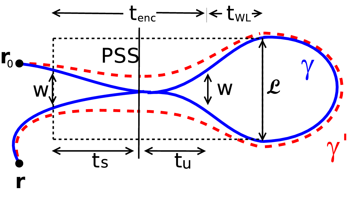
As pointed out in Ref. [12] the densities should be multiplied by a Heaviside function ensuring that the contribution exists only for times larger than the encounter time. Only trajectories that are closer than a distance $w$ to themselves will have an enhanced probability of staying. Correlated trajectories should come closer to themselves than a distance $c^{2}$ in phase space related to the opening, i.e., we place the PSS only in the region were the stretches are closer than a distance $w$ in configuration space, see Fig. 4. Moreover, on the right hand side of the encounter, the stretches should separate at least a distance ${\mathcal{L}}$ in order to close themselves. This is because the two almost parallel momenta at the encounter have to grow until they are in exactly opposite directions, which requires that the stretches are no longer linearizable along each other and therefore should be separated by a distance comparable to the system size. The duration of the trajectory should then be at least $2t_{\rm enc}+2t_{WL}$ , where

t_{\rm WL}=\lambda^{-1}\ln(\mathcal{L}/w)

(92)

is the time it takes for the stretches to be separated by a distance ${\mathcal{L}}$ when they are initially separated by a distance $w$ . The weight function is slightly modified by this minimal time and by ensuring that the time is long enough in order to have such an encounter. Thus

w^{\rm 2ll}(u,s,t)=\frac{(t-2(t_{\rm enc}+t_{\rm WL}))^{2}}{2\Omega t_{\rm enc}}\theta(t-2t_{\rm enc}-2t_{\rm WL})\,,

(93)

and the classical survival probability is modified by ${\rm e}^{t_{\rm enc}/\tau_{d}}$ . In Appendix B the evaluation of the integral can be found, together with the calculation for the 1ll case. The total contribution can then be written as

C^{1,\rm 2ll+1ll}_{\tau_{E}}(\omega)=\frac{4}{N^{2}}{\rm e}^{-\frac{\tau_{E}^{c}}{\tau_{d}}}Re\left\{\frac{(1-i\Gamma)^{3}}{(1+\Gamma^{2})^{3}}{\rm e}^{-2i\omega\tau_{E}^{e}}\right\}\,,

(94)

where $\Gamma=\omega\tau_{d}$ , $N=t_{H}/\tau_{d}$ and $2\tau_{E}^{e}=\tau_{E}^{\rm c}+\tau_{E}^{\rm o}$ . Taking the Fourier transform this corresponds to a dependence in $Z^{1}(t)$ as

Z^{\rm 1,2ll+1ll}_{\tau_{E}}(t)=e^{-t/\tau_{d}}e^{\tau_{E}^{o}/\tau_{d}}\frac{(t-2\tau_{E}^{e})^{2}}{\tau_{d}t_{H}}\theta(t-2\tau_{E}^{e}),

(95)

consistent with [12] for the decay. Here we see two competing effects, on one hand if the Ehrenfest time is too large, loops can not be formed, $\theta(t-2\tau_{E}^{e})=0$ , and there are no quantum contributions. On the other hand, if the time is long enough so that the loops can occur, i.e. if $t>2\tau_{E}^{e}$ , the probability of staying is enhanced by a factor $e^{\tau_{E}^{o}/\tau_{d}}$ compared to generic orbits, revealing the enhanced classical survival probability due to the encounter. In the energy domain, the auto-correlation function $C(\omega)$ , Eq. (94), shows an exponential suppression of quantum effects depending on the Ehrenfest time of the closed system, similar to the exponential suppression of weak localization in transport in mesoscopic systems [47, 48, 18, 21, 20, 22], while additionally oscillations in $\omega$ with a period given by $\tau_{E}^{e}$ are expected.

Let us consider now the Ehrenfest time dependence of the first quantum correction to $C^{2}(\omega)$ . A calculation of the Ehrenfest time dependence of the spectral form factor of closed systems was performed in Ref. [16]. We follow here a similar approach, taking into account now the opening of the system, and the two different Ehrenfest time scales. In this situation the stretches are required to be separated by a distance $\mathcal{L}$ also on the left and right hand side of the encounter. Therefore the minimal time for the orbits is $2t_{\rm enc}+4t_{\rm WL}$ .

The first quantum correction to the spectral form factor results from orbits sketched in Fig. 5 [13] denoted in the following by $(2)^{1}$ . The corrected weight function is then given by

w^{(2)^{1}}(u,s,t)=\frac{t(t-2t_{\rm enc}-4t_{\rm WL})}{2\Omega t_{\rm enc}}\theta(t-2t_{\rm enc}-4t_{\rm WL})\,.

(96)

The contribution to the autocorrelation function, after shifting the time integration by $2t_{\rm enc}$ , can be written as

	$\displaystyle C^{\rm 2,(2)^{1}}_{\tau_{E}}(\omega)$	$\displaystyle=$	$\displaystyle\frac{4}{t_{H}^{3}}Re\int_{4t_{\rm WL}}^{\infty}{\rm e}^{-(1+i\omega\tau_{d})t/\tau_{d}}$		(97)
			$\displaystyle\times(t-4t_{\rm WL})I^{\rm(2)^{1}}(\omega,t),$		(97)

with

	$\displaystyle I^{\rm(2)^{1}}(\omega,t)$	$\displaystyle=$	$\displaystyle\frac{1}{\pi\hbar}\int_{0}^{c}du\int_{0}^{c}ds{\rm e}^{\frac{i}{\hbar}us}\frac{(t+2t_{\rm enc})^{2}}{t_{\rm enc}}$		(98)
			$\displaystyle\times{\rm e}^{-(1+2i\omega\tau_{d})t_{\rm enc}/\tau_{d}}.$		(98)

The integrals can be performed as before, yielding

	$\displaystyle C^{\rm 2,(2)^{1}}_{\tau_{E}}(\omega)$	$\displaystyle=$	$\displaystyle\frac{8{\rm e}^{(\tau_{E}^{o}-2\tau_{E}^{c})/\tau_{d}}}{N^{3}}Re\left[{\rm e}^{-2i\omega\tau_{E}^{c}}\!\left(\frac{(1-2i\Gamma)}{(1+i\Gamma)^{4}}\right.\right.$		(99)
			$\displaystyle\left.\left.-\frac{4i\omega\tau_{E}^{c}}{(1+i\Gamma)^{3}}-\frac{2\tau_{E}^{c\,2}(1+2i\Gamma)}{\tau_{d}^{2}(1+i\Gamma)^{2}}\right)\right],$		(99)

where $\Gamma=\omega\tau_{d}$ again. Taking the Fourier transform, the result for the spectral form factor of the open system is

	$\displaystyle Z_{\tau_{E}}^{\rm 2,(2)^{1}}(t)$	$\displaystyle=$	$\displaystyle{\rm e}^{-t/\tau_{d}}{\rm e}^{\tau_{E}^{o}/\tau_{d}}\theta(t-2\tau_{E}^{c})$		(100)
			$\displaystyle\times\left[-2\frac{t^{2}}{t_{H}^{2}}\left(1+\frac{\tau_{E}^{c}}{\tau_{d}}\right)+\frac{t^{3}}{\tau_{d}t_{H}^{2}}\right]\,.$		(100)

If $\tau_{d}\to\infty$ and the system is closed, Eq. (100) is consistent with Ref. [16]. Similarly as for Eq. (95) the step function ensures that only trajectories longer than $2\tau_{E}^{c}$ give a contribution, which are larger than $2\tau_{E}^{e}$ since the orbits have to close themselves. For those orbits the contribution is enhanced by ${\rm e}^{\tau_{E}^{o}/\tau_{d}}$ , again showing the enhanced survival probability for periodic orbits with a self-encounter. As in Eq. (94), Eq. (99) shows that the quantum corrections in the cross-section autocorrelation function are exponentially suppressed due to the minimal time that self-encounters require. In the case of periodic orbits, the suppression is stronger (since $\tau_{E}^{c}>\tau_{E}^{o}$ ).

VIII Conclusions and Outlook

We have presented a detailed semiclassical analysis of the quantum survival probability and of photofragmentation cross-section statistics, including higher order corrections. We have demonstrated how interference contributions associated with certain trajectory pairs provide the key to understanding and deducing quantum corrections to the leading classical features in chaotic decay. We have seen in the case of the survival probability that the initial semiclassical treatment introduced in Ref. [12] for localized wave packets can be extended to non-localized ones by assuming a local time average, which allows us to treat in the arising double sums of trajectories pairs only those that are correlated. Apart from the standard off-diagonal contributions, it proves necessary to include further, so-called one-leg-loop, diagrams in order to recover unitary, expressed via the normalization of the wave function when the system is closed. Trajectories with multiple encounters of several stretches lead to higher order corrections for systems with and without time reversal symmetry, for which again it is necessary to take into account the corresponding one-leg-loops as well as diagrams where both the initial and final points are inside encounter regions (which are not the same). Taking into account all the different allowed structures, depending on the general symmetries of the problem, we can reproduce RMT-type results presented in Ref. [10], where the survival probability was calculated using supersymmetry techniques. Moreover, our approach can be further extended to also include systems with spin-orbit interaction, which corresponds to the symplectic RMT ensemble. We have also considered mesoscopic survival probability fluctuations through their variance and could explicitly show that they are non-universal, that is, that the variance depends on the spatial width of the initial (coherent) state.

In the second part of the paper, we presented in detail an application of this approach to a different field, namely photodissociation and photoionization processes. We considered correlations in frequency of photofragmentation cross-sections. Its Fourier transform, the corresponding photofragmentation form factor can be semiclassically expressed as the sum of (twice) the survival probability, related to open trajectories, and the spectral form factor of the open system, related to the set of periodic orbits that are trapped in the open system. We have semiclassically computed the photofragmentation form factor to high order in $t/t_{H}$ and moreover considered Ehrenfest time effects.

According to previous numerical results [12] there are clear indications for the importance of Ehrenfest-time effects in decay processes, leading to a shift in time of the quantum corrections. In the context of photofragmentation, we have shown here that quantum corrections of the photodissociation form factor are also distinctly shifted in time (with a stronger shift for periodic orbit contributions). This time shift translates into an exponential suppression of quantum effects in the cross-section correlator, if the Ehrenfest time is comparable to the typical life time of the intermediate atomic or molecular resonant states in the fragmentation process. Our semiclassical results also predict a frequency modulation of the correlator with period given by the Ehrenfest time.

The semiclassical approach developed here to treat decay processes can be extended to address other quantities where semiclassics so far was limited by the diagonal approximation. One example is the problem of the Loschmidt echo or fidelity, respectively, where a semiclassical treatment along similar lines as the one presented here allows one to calculate quantum corrections to the fidelity decay [51].

The present approach is still limited to times smaller than the Heisenberg time. An extension to longer times beyond $t_{H}$ remains as a challenging open problem of semiclassics for open quantum systems.

IX Acknowledgments

We thank P. Brouwer, A. Goussev, C. Petitjean and D. Savin for helpful discussions. We acknowledge funding by DFG under GRK 638.

Appendix A Appendix A: Higher order contributions to the decay rate in the orthogonal case

$\boldsymbol{v}$	$L$	$V$	$N(\boldsymbol{v})$	$\mathcal{N}_{l_{1},l_{2}}(\boldsymbol{v})$	$\mathcal{N}_{l_{1},l_{V}}(\boldsymbol{v})$	$\mathcal{N}_{l_{V-1},l_{V}}(\boldsymbol{v})$
$(2)^{1}$	2	1	1
$(2)^{2}$	4	2	5	4
$(3)^{1}$	3	1	4
$(2)^{3}$	6	3	41	36
$(2)^{1}(3)^{1}$	5	2	60	40
$(4)^{1}$	4	1	20
$(2)^{4}$	8	4	509	468
$(2)^{2}(3)^{1}$	7	3	1092	228	672
$(2)^{1}(4)^{1}$	6	2	504	296
$(3)^{2}$	6	2	228	148
$(5)^{1}$	5	1	148
$(2)^{5}$	10	5	8229	7720
$(2)^{3}(3)^{1}$	9	4	23160	8220	12256
$(2)^{2}(4)^{1}$	8	3	12256	1884	7480
$(2)^{1}(3)^{2}$	8	3	10960	5024		3740
$(2)^{1}(5)^{1}$	7	2	5236	2696
$(3)^{1}(4)^{1}$	7	2	4396	2696
$(6)^{1}$	6	1	1348
$(2)^{6}$	12	6	166377	158148
$(2)^{4}(3)^{1}$	11	5	579876	266040	265056
$(2)^{3}(4)^{1}$	10	4	331320	93456	186160
$(2)^{2}(3)^{2}$	10	4	443400	41792	249216	93080
$(2)^{2}(5)^{1}$	9	3	167544	19872	98712
$(2)^{1}(3)^{1}(4)^{1}$	9	3	280368	49576	66240	98712
$(3)^{3}$	9	3	41792	33120
$(2)^{1}(6)^{1}$	8	2	65808	30208
$(3)^{1}(5)^{1}$	8	2	52992	30208
$(4)^{2}$	8	2	24788	15104
$(7)^{1}$	7	1	15104

Table 2: The number of trajectory pairs and the number linking certain encounters for systems with time reversal symmetry.

Table 2 allows us to obtain the following semiclassical corrections to $\rho^{\rm cl}=\mathrm{e}^{-\frac{t}{\tau_{d}}}$ for the orthogonal case:

\bar{\rho}_{1}(t)=\frac{\mathrm{e}^{-\frac{t}{\tau_{d}}}}{t_{H}}\left(\frac{t^{2}}{2\tau_{d}}\right),

(101)

\bar{\rho}_{2}(t)=\frac{\mathrm{e}^{-\frac{t}{\tau_{d}}}}{t_{H}^{2}}\left(-\frac{t^{3}}{3\tau_{d}}+\frac{5t^{4}}{24\tau_{d}^{2}}\right),

(102)

\bar{\rho}_{3}(t)=\frac{\mathrm{e}^{-\frac{t}{\tau_{d}}}}{t_{H}^{3}}\left(\frac{t^{4}}{3\tau_{d}}-\frac{11t^{5}}{30\tau_{d}^{2}}+\frac{41t^{6}}{720\tau_{d}^{3}}\right),

(103)

\bar{\rho}_{4}(t)=\frac{\mathrm{e}^{-\frac{t}{\tau_{d}}}}{t_{H}^{4}}\left(-\frac{2t^{5}}{5\tau_{d}}+\frac{7t^{6}}{12\tau_{d}^{2}}-\frac{29t^{7}}{168\tau_{d}^{3}}+\frac{509t^{8}}{40320\tau_{d}^{4}}\right),

(104)

	$\displaystyle\bar{\rho}_{5}(t)$	$\displaystyle=$	$\displaystyle\frac{\mathrm{e}^{-\frac{t}{\tau_{d}}}}{t_{H}^{5}}\left(\frac{8t^{6}}{15\tau_{d}}-\frac{14t^{7}}{15\tau_{d}^{2}}+\frac{31t^{8}}{80\tau_{d}^{3}}\right.$		(105)
			$\displaystyle\qquad\qquad\left.-\frac{271t^{9}}{5040\tau_{d}^{4}}+\frac{2743t^{10}}{1209600\tau_{d}^{5}}\right),$		(105)

	$\displaystyle\bar{\rho}_{6}(t)$	$\displaystyle=$	$\displaystyle\frac{\mathrm{e}^{-\frac{t}{\tau_{d}}}}{t_{H}^{6}}\left(-\frac{16t^{7}}{21\tau_{d}}+\frac{5099t^{8}}{3360\tau_{d}^{2}}-\frac{4469t^{9}}{5670\tau_{d}^{3}}+\frac{437t^{10}}{2800\tau_{d}^{4}}\right.$		(106)
			$\displaystyle\qquad\qquad\left.-\frac{28001t^{11}}{2217600\tau_{d}^{5}}+\frac{55459t^{12}}{159667200\tau_{d}^{6}}\right).$		(106)

Appendix B Appendix B: Ehrenfest time dependence of the leading quantum correction to the cross-section correlation $C(\omega)$

Substituting the expressions (92) and (93) into Eq. (91) and shifting the time integral by $2t_{\rm enc}+2t_{\rm WL}$ we have for the 2ll correction to the photo cross-section correlation

C^{1,\rm 2ll}_{\tau_{E}}(\omega)=\frac{4}{t_{H}^{2}}Re\int_{0}^{\infty}\,t^{2}\,{\rm e}^{-(1+i\omega\tau_{d})(t+2t_{\rm WL})/\tau_{d}}I^{\rm 2ll}(\omega)dt

(107)

with

I^{\rm 2ll}(\omega)=\frac{1}{\pi\hbar}\int_{0}^{c}du\int_{0}^{c}ds\frac{{e}^{\frac{i}{\hbar}us}}{t_{\rm enc}}{\rm e}^{t_{\rm enc}/\tau_{d}}{\rm e}^{-2(1+i\omega\tau_{d})t_{\rm enc}/\tau_{d}}.

(108)

Upon change of variables, $x=us/c^{2}$ and $\sigma=c/u$ , we obtain

I^{\rm 2ll}(\omega)=\frac{r\lambda}{\pi}\int_{0}^{1}dx\cos(rx)x^{(1+2i\omega\tau_{d})/(\lambda\tau_{d})}\,,

(109)

where $r=c^{2}/\hbar$ , and the integral over $\sigma$ has already been performed. We compute the remaining integral by partial integration, neglecting highly oscillating terms in the limit $\hbar\to 0$ while keeping $\tau_{E}^{o}/\tau_{d}$ (Eq. (89)) and $\tau_{E}^{c}/\tau_{d}$ (Eq. (90)) finite. We find

I^{\rm 2ll}(\omega)=-\frac{(1+2i\omega\tau_{d})}{2\tau_{d}}{\rm e}^{\tau_{E}^{o}/\tau_{d}}e^{-2(1+i\omega\tau_{d})\tau_{E}^{o}/\tau_{d}},

(110)

with Ehrenfest time $\tau_{E}^{\rm o}\!=\!\lambda^{-1}\!\ln(c^{2}/\hbar)$ . Then Eq. (107) gives

C^{1,\rm 2ll}_{\tau_{E}}(\omega)=-\left(\frac{2\tau_{d}}{t_{H}}\right)^{2}{\rm e}^{-\frac{\tau_{E}^{c}}{\tau_{d}}}Re\left[\frac{1+2i\omega\tau_{d}}{(1+i\omega\tau_{d})^{3}}{\rm e}^{-2i\omega\tau_{E}^{e}}\right].

(111)

Here we used that from the definitions of $\tau_{E}^{\rm o}$ and $t_{\rm WL}$ follows $\tau_{E}^{\rm o}+2t_{\rm WL}=\tau_{E}^{\rm c}$ , and we introduced $\tau_{E}^{e}=(\tau_{E}^{\rm c}+\tau_{E}^{\rm o})/2$ .

A corresponding calculation can be performed for the 1ll case, where

C^{1,\rm 1ll}_{\tau_{E}}(\omega)=\frac{16}{t_{H}^{2}}Re\int_{0}^{\infty}\,t\,{\rm e}^{-(1+i\omega\tau_{d})(t+2t_{WL})/\tau_{d}}I^{\rm 1ll}(\omega)dt

(112)

with

	$\displaystyle I^{\rm 1ll}(\omega)$	$\displaystyle=$	$\displaystyle\frac{1}{\pi\hbar}\int_{0}^{c}du\int_{0}^{c}ds\int_{0}^{\lambda^{-1}\ln(c/\|s\|)}dt^{\prime}\frac{{e}^{\frac{i}{\hbar}us}}{t_{\rm enc}}$		(113)
			$\displaystyle\times{\rm e}^{t_{\rm enc}/\tau_{d}}{\rm e}^{-2(1+i\omega\tau_{d})t_{\rm enc}/\tau_{d}},$		(113)

and $t_{\rm enc}=t^{\prime}+\lambda^{-1}\ln(c/|u|)$ . With the change of variables $x=us/c^{2}$ and $\sigma=c/u$ and $t^{\prime\prime}=t^{\prime}+\lambda^{-1}\ln(c/|u|)$ , we obtain

I^{\rm 1ll}(\omega)=-\frac{\lambda r\tau_{d}}{\pi(1+2i\omega\tau_{d})}\int_{0}^{1}dx\cos(rx)x^{\frac{1}{\lambda\tau_{d}}(1+2i\omega\tau_{d})}\ .

(114)

The integral can be evaluated as before, neglecting higher-order terms. Together with $C^{1,\rm 2ll}_{\tau_{E}}(\omega)$ from Eq. (111) we find

C^{1,\rm 2ll+1ll}_{\tau_{E}}(\omega)=4\frac{\tau_{d}^{2}}{t_{H}^{2}}{\rm e}^{-\frac{\tau_{E}^{c}}{\tau_{d}}}Re\left[\frac{(1-i\omega\tau_{d})^{3}}{(1+(\omega\tau_{d})^{2})^{3}}{\rm e}^{-2i\omega\tau_{E}^{e}}\right]\,,

(115)

which corresponds to Eq. (94).

References

[1] G. Bacher, R. Weigand, J. Seufert, V. D. Kulakovskii, N. A. Gippius, A. Forchel, K. Leonardi, and D. Hommel, Phys. Rev. Lett. 83, 4417 (1999).
[2] R. Kumar, A. S. Vengurlekar, A. Venu Gopal, T. Mélin, F. Laruelle, B. Etienne, and J. Shah, Phys. Rev. Lett. 81, 2578 (1998).
[3] G. Stania and H. Walther, Phys. Rev. Lett. 95, 194101 (2005).
[4] T. Baumert, M. Grosser, R. Thalweiser, and G. Gerber, Phys. Rev. Lett. 67, 3753 (1991).
[5] R. Schinke, Photodissociation Dynamics (Cambridge University Press, Cambridge, 1993).
[6] V. Milner, J. L. Hanssen, W. C. Campbell, and M. G. Raizen, Phys. Rev. Lett. 86, 1514 (2001); N. Friedman, A. Kaplan, D. Carasso, and N. Davidson, ibid, 1518 (2001);
[7] J. U. Nöckel and A. D. Stone, Nature (London) 385, 45 (1997); T. Harayama, P. Davis, and K. S. Ikeda, Phys. Rev. Lett. 90, 063901 (2003); W. Fang, A. Yamilov, and H. Cao, Phys. Rev. A 72, 023815 (2005); J. Wiersig and M. Hentschel, Phys. Rev. Lett. 100, 033901 (2008).
[8] G. Casati, G. Maspero, and D. L. Shepelyansky, Phys. Rev. E 56, R6233 (1997); G. Casati, I. Guarneri, and G. Maspero, Phys. Rev. Lett. 84, 63 (2000); G. Casati, G. Maspero, and D. L. Shepelyansky, Phys. Rev. Lett. 82, 524 (1999).
[9] K. M. Frahm, Phys. Rev. E 56, R6237 (1997).
[10] D. V. Savin and V. V. Sokolov, Phys. Rev. E 56, R4911 (1997); D. V. Savin and H.-J. Sommers, Phys. Rev. E 68, 036211 (2003).
[11] M. Puhlmann, H. Schanz, T. Kottos, and T. Geisel, Europhys. Lett. 69, 313 (2005).
[12] D. Waltner, M. Gutiérrez, A. Goussev, and K. Richter, Phys. Rev. Lett. 101, 174101 (2008).
[13] M. Sieber and K. Richter, Phys. Scr. T90, 128 (2001); M. Sieber, J. Phys. A 35, L613 (2002).
[14] S. Müller, Eur. Phys. J. B 34, 305 (2003); M. Turek and K. Richter, J. Phys. A 36, L455 (2003); D. Spehner, J. Phys. A 36, 7269 (2003).
[15] S. Müller, S. Heusler, P. Braun, F. Haake, and A. Altland, Phys. Rev. Lett. 93, 014103 (2004); S. Müller, S. Heusler, P. Braun, F. Haake, and A. Altland, Phys. Rev. E 72, 046207 (2005); S. Heusler, S. Müller, A. Altland, P. Braun, and F. Haake, Phys. Rev. Lett. 98 044103 (2007); S. Müller, Periodic orbit approach to universality in quantum chaos, PhD thesis, arXiV:nlin/0512058v1 (2005).
[16] P. W. Brouwer, S. Rahav, and C. Tian, Phys. Rev. E 74, 066208 (2006).
[17] K. Richter and M. Sieber, Phys. Rev. Lett. 89, 206801 (2002).
[18] İ. Adagideli, Phys. Rev. B 68, 233308 (2003).
[19] S. Heusler, S. Müller, P. Braun, and F. Haake, Phys. Rev. Lett. 96, 066804 (2006); S. Müller, S. Heusler, P. Braun, and F. Haake, New J. Phys. 9, 12 (2007).
[20] P. W. Brouwer and S. Rahav, Phys. Rev. B 74, 075322 (2006).
[21] S. Rahav and P. W. Brouwer, Phys. Rev. Lett. 96, 196804 (2006).
[22] Ph. Jacquod and R. S. Whitney, Phys. Rev. B 73, 195115 (2006).
[23] J. Kuipers and M. Sieber, Phys. Rev. E 77, 046219 (2008).
[24] R. S. Whitney, Phys. Rev. B 75, 235404 (2007).
[25] O. Agam, Phys. Rev. E 61, 1285 (2000).
[26] B. Eckhardt, S. Fishman, and I. Varga, Phys. Rev. E 62, 7867 (2000).
[27] M. Gutzwiller, Chaos in Classical and Quantum Mechanics (Springer, New York, 1990).
[28] F. M. Cucchietti, H. M. Pastawski, and R. A. Jalabert, Phys. Rev. B 70, 035311 (2004).
[29] M. Sieber, J. Phys. A 32, 7679 (1999).
[30] J. Kuipers and M. Sieber, Nonlinearity 20, 909 (2007).
[31] O. Zaitsev, D. Frustaglia, and K. Richter, Phys. Rev. Lett. 94, 026809 (2005); Phys. Rev. B 72, 155325 (2005); O. Zaitsev and K. Richter, Mat. Science-Poland 22, 469 (2004).
[32] J. Bolte and D. Waltner, Phys. Rev. B 76, 075330 (2007).
[33] J. Bolte and S. Keppeler, Ann. Phys. (N. Y.) 274, 125 (1999).
[34] N. Argaman, Phys. Rev. Lett. 75, 2750 (1995); Phys. Rev. B 53, 7035 (1996).
[35] A result corresponding to (67) has been independently obtained by P. W. Brouwer (private communication).
[36] K. P. Lawley (Ed.), Photodissociation and Photoionization (Wiley, New York, 1995).
[37] Y. V. Fyodorov and Y. Alhassid, Phys. Rev. A 58 R3375 (1998).
[38] Y. Alhassid and Y. V. Fyodorov, J. Phys. Chem. A 102, 9577 (1998).
[39] Taking in Eq. (8) of Y. Alhassid, Y. V. Fyodorov, T. Gorin, W. Ihra, and B. Mehlig, Phys. Rev. A 73 042711 (2006) the limit of no direct coupling to the continuum and $t\gg t_{H}$ leads to Eq. (84).
[40] T. Ericson, Phys. Rev. Lett. 5, 430 (1960); Phys. Lett. 4, 258 (1963); Ann. Phys. 23, 390 (1963).
[41] P. von Brentano, J. Ernst, O. Häusser, T. Mayer-Kuckuk, A. Richter, and W. von Witsch, Phys. Lett. 9, 48 (1964).
[42] B. Eckhardt and C. Jung, J. Phys. A 19, L829 (1986); B. Eckhardt, J. Phys. A 20, 5971 (1987); C. Jung and H. Scholz, J. Phys. A 20, 3607 (1987).
[43] J. Main and G. Wunner, J. Phys. B 27, 2835 (1994); V. V. Flambaum, A. A. Gribakina, and G. F. Gribakin, Phys. Rev. A 54, 2066 (1996).
[44] J. Madroñero and A. Buchleitner, Phys. Rev. Lett. 95, 263601 (2005).
[45] T. Gorin, J. Phys. A 38, 10805 (2005).
[46] B. V. Chirikov, F. M. Izrailev, and D. L. Shepelyansky, Sov. Sci. Rev. Sect. C 2, 209 (1981).
[47] I. L. Aleiner and A. I. Larkin, Phys. Rev. B 54, 14423 (1996).
[48] O. Yevtushenko, G. Lütjering, D. Weiss, and K. Richter, Phys. Rev. Lett. 84, 542 (2000).
[49] P. Jacquod, İ. Adagideli, and C.W.J. Beenakker, Phys. Rev. Lett. 89, 154103 (2002).
[50] H. Schomerus and J. Tworzydło, Phys. Rev. Lett. 93, 154102 (2004).
[51] B. Gutkin, D. Waltner, M. Gutiérrez, J. Kuipers, and K. Richter, in preparation (2008).

Semiclassical Theory for Decay and Fragmentation Processes in Chaotic Quantum Systems

Abstract

pacs

I I. Introduction

II II. Semiclassical approach to the survival probability

III III. Survival probability: Leading order weak localization-type contributions

III.1 Two-leg-loops

III.2 One-leg-loops

IV IV. Survival probability: Higher order contributions for the GUE, GOE and GSE cases

IV.1 Case A

IV.2 Case B

IV.3 Case C

IV.4 Unitary case

IV.5 Orthogonal case

IV.6 Spin-orbit interaction and the symplectic case

V V. Variance of the Decay

VI VI. Statistics of photofragmentation cross-sections

VI.1 Open trajectory contributions

VI.2 Periodic orbit contributions

VII VII. Ehrenfest time effects in photofragmentation statistics

VIII Conclusions and Outlook

IX Acknowledgments

Appendix A Appendix A: Higher order contributions to the decay rate in the orthogonal case

Appendix B Appendix B: Ehrenfest time dependence of the leading quantum correction to the cross-section correlation C⁡(ω)C(\omega)

References

Semiclassical Theory for Decay and Fragmentation Processes
in Chaotic Quantum Systems

Appendix B Appendix B: Ehrenfest time dependence of the leading quantum correction to the cross-section correlation $C(\omega)$