Casimir interaction among heavy fermions in the BCS-BEC crossover

Consider a two-species Fermi gas with unequal masses $M$ and $m$ interacting by an interspecies short-range interaction. When the mass ratio is large $M/m\gg 1$, we can employ the Born-Oppenheimer approximation to compute the interaction energy of heavy fermions immersed in the Fermi sea of light fermions. Here we concentrate on the case of two heavy fermions. The formula for a general number of heavy fermions is derived in Appendix A using the functional integral method. The wave function of a light fermion interacting with two heavy fermions fixed at positions ${\bm{x}}_{1}$ and ${\bm{x}}_{2}$ satisfies the Schrödinger equation (here and below $\hbar=1$):

The interspecies short-range interaction between the light and heavy fermions is taken into account by imposing the short-range boundary condition; $\Psi({\bm{y}}\to{\bm{x}}_{i})\propto\frac{1}{|{\bm{y}}-{\bm{x}}_{i}|}-\frac{1}{a}+O(|{\bm{y}}-{\bm{x}}_{i}|)$, where $a$ is the $s$-wave scattering length. Below we determine the energy spectrum of the light fermion both for bound states and continuum states as a function of $a$ and the separation between the heavy fermions ${\bm{r}}\equiv{\bm{x}}_{1}-{\bm{x}}_{2}$.

For the bound state $E=-\frac{\kappa^{2}}{2m}<0$, the solution of Eq. (1) takes the form

where $\pm$ is the parity of the wave function. The upper (lower) sign corresponds to the even (odd) parity. From the short-range boundary condition, we obtain the equation

The solution to this equation exists when $|{\bm{r}}|/a>\mp 1$ and is given by

where $W(z)$ is the Lambert function satisfying $z=W(z)e^{W(z)}$. Accordingly we find the following binding energy depending on $a$ and $|{\bm{r}}|$:

for $|{\bm{r}}|/a>\mp 1$.

For the continuum state $E=\frac{k^{2}}{2m}>0$, the solution of Eq. (1) takes the form

where $0\leq\delta_{\pm}\leq\pi$ is the phase shift. From the short-range boundary condition, we obtain the equation

The solution to this equation is easily found to be

We then suppose that the system is confined in a large sphere with a radius $R\gg|{\bm{r}}|$ and the two heavy fermions are located near its center; ${\bm{x}}_{1}=\frac{{\bm{r}}}{2}$ and ${\bm{x}}_{2}=-\frac{{\bm{r}}}{2}$. By imposing $\Psi_{\pm}(|{\bm{y}}|\to R)\to 0$ at the boundary of the sphere, the momentum $k$ is discretized as

with $n=1,2,3,\ldots$. Therefore the energy level becomes

Now we fill the above-obtained energy levels with the light fermions. The total energy of such a system is given by

where $2N$ is the number of interacting light fermions in the continuum states. We compare the energy of the interacting system with that in the noninteracting limit,

and define the energy reduction as $\Delta E(|{\bm{r}}|)\equiv E-E_{\mathrm{free}}$. Then we take the thermodynamic limit $N,R\to\infty$ with the Fermi momentum of the light fermions $k_{\mathrm{F}}\equiv N\pi/R$ fixed. If we notice that the summation over $n$ is dominated by $n\sim N\gg 1$ and neglect small corrections of $O(1/N)$, we obtain the following simple expression for the energy reduction:

We note that the phase shifts given in Eq. (8) are defined to be in the range $0\leq\delta_{\pm}(k)\leq\pi$. The same result can be obtained on a more general footing by using the functional integral method (see Appendix A).

When the two heavy fermions are infinitely separated, the energy reduction approaches

where $\mu_{\mathrm{single}}<0$ is the chemical potential of a single heavy fermion immersed in the Fermi sea of light fermions [20]:

The energy reduction with $2\mu_{\mathrm{single}}$ subtracted is regarded as the interaction energy of the two heavy fermions:

$V(|{\bm{r}}|)$ represents the effective interaction between two heavy fermions induced by the interaction with the Fermi sea of light fermions. We note that the chemical potential of light fermions $\mu_{l}\equiv\frac{k_{\mathrm{F}}^{\,2}}{2m}$ is fixed here instead of their particle number.

It is convenient to measure the interaction energy $V(r)$ in units of the Fermi energy of light fermions and introduce a dimensionless function $v(k_{\mathrm{F}}r)$ as

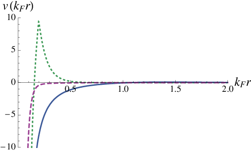
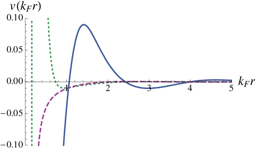
$v(k_{\mathrm{F}}r)$ is a function of the separation between the heavy fermions $k_{\mathrm{F}}r$ and also the $s$-wave scattering length $ak_{\mathrm{F}}$. $v(k_{\mathrm{F}}r)$ for three typical values of $(ak_{\mathrm{F}})^{-1}=-5,\,0,\,5$ are plotted in Fig. 1. One can see the smooth evolution of the effective interaction between the two heavy fermions as a function of $(ak_{\mathrm{F}})^{-1}$ in Fig. 2. In the BCS regime $(ak_{\mathrm{F}})^{-1}\lesssim-1$, the effective interaction is attractive at $r\lesssim|a|$ and has a tiny oscillatory behavior at $r\gtrsim|a|$. This oscillatory behavior grows toward the unitarity limit $(ak_{\mathrm{F}})^{-1}\approx 0$ and makes a small hump at $r\simeq k_{\mathrm{F}}^{-1}$ (see the left panel of Fig. 2). This hump further grows in the BEC regime $(ak_{\mathrm{F}})^{-1}\gtrsim 1$ and eventually develops a repulsive core at $r\simeq a$ (see the right panel of Fig. 2).

It is worthwhile to compare our nonperturbative result (16) with the perturbative calculation of the effective interaction in the BCS limit $a\to-0$. In the BCS limit $|a|\ll r,k_{\mathrm{F}}^{-1}$, we have $\kappa_{\pm}\to 0$ and the phase shift

Thus we can find the interaction energy to be

which has the same form as the Ruderman-Kittel-Kasuya-Yosida interaction between magnetic impurities in a Fermi liquid [21]. Accordingly the Fourier transform of the effective interaction $V(|{\bm{r}}|)$ in the BCS limit becomes

which correctly reproduces the effective interaction to the leading order in $a$ obtained in Ref. [12] ¹¹ 1 For unequal masses, the effective interaction in the BCS limit becomes $\tilde{V}(|{\bm{p}}|)=-\left[\frac{2\pi(m+M)a}{mM}\right]^{2}\frac{mk_{\mathrm{F}}}{2\pi^{2}}L\!\left(\frac{|{\bm{p}}|}{2k_{\mathrm{F}}}\right)$, where $L(z)=\frac{1}{2}+\frac{1-z^{2}}{4z}\ln\!\left|\frac{1+z}{1-z}\right|$ is the static Lindhard function. The limit of large mass ratio $M/m\gg 1$ coincides with Eq. (20). as it should be. Our nonperturbative result (16) can go beyond the perturbative BCS regime to the strongly interacting unitary regime in a controlled way by utilizing $M/m\gg 1$.

Analytic expressions of $v(k_{\mathrm{F}}r)$ in various limits are obtained in Appendix B.

The physics of heavy fermions immersed in the Fermi sea of light fermions is described by the Hamiltonian

where $\mu_{h}$ is the chemical potential of heavy fermions measured from $\mu_{\mathrm{single}}$. Strictly speaking, the pairwise interaction $V(|{\bm{r}}|)$ obtained in the previous section [Eq. (16)] is valid only if there are two heavy fermions in the system. This is because the Casimir interaction energy is not pairwise additive and also because if heavy fermions have a finite density, it will perturb the Fermi sea of light fermions and thus affect the effective interaction $V(|{\bm{r}}|)$. However, in the dilute limit $\sqrt{2M\mu_{h}}\ll k_{\mathrm{F}}$, we expect that the above Hamiltonian is a good approximation to the system of heavy fermions because the probability to find a third heavy fermion near the two heavy fermions becomes small in the dilute system [22]. Indeed we will confirm in Appendix A that the Casimir interaction among more than two heavy fermions at large separations can be evaluated quite accurately as a sum of pairwise interactions between each of the two heavy fermions. This result also supports the use of our Hamiltonian (21) to describe the physics of dilute heavy fermions immersed in the Fermi sea of light fermions.

Another issue to be addressed is the instability of the system. When the mass ratio $M/m$ exceeds the critical value 13.6 in pure 3D [23] or 6.35 in the 2D-3D mixture [18], the system will not be stable due to the Efimov effect. Therefore we need to assume the mass ratio to be large but smaller than the above critical value. For such a mass ratio, the effective interaction $V(|{\bm{r}}|)$ obtained in the Born-Oppenheimer approximation is no longer exact but can be considered as a good approximation to the exact one.

One of predictions we can derive from the Hamiltonian (21) is a pairing between the heavy fermions. The pairing gap of heavy fermions $\Delta_{\bm{p}}$ is defined to be

where $\tilde{\psi}_{h}({\bm{p}})$ is the Fourier transform of $\psi_{h}({\bm{x}})$ and $\tilde{V}(|{\bm{p}}-{\bm{q}}|)$ is the Fourier transform of $V(|{\bm{r}}|)$ [see Eq. (20)]. Because of the Fermi statistics of heavy fermions, the pairing gap has to have an odd parity; $\Delta_{-{\bm{p}}}=-\Delta_{{\bm{p}}}$. The standard mean-field calculation leads to the self-consistent gap equation

Here $E_{\bm{p}}=\sqrt{\left(\frac{{\bm{p}}^{2}}{2M}-\mu_{h}\right)^{2}+|\Delta_{\bm{p}}|^{2}}$ is the quasiparticle energy and $n_{\mathrm{F}}(E_{\bm{p}})=1/\left(e^{E_{\bm{p}}/T}+1\right)$ is the Fermi-Dirac distribution function at temperature $T$.

When the coupling between different partial waves can be neglected, we can solve the gap equation (23) easily by using the weak-coupling approximation ²² 2 The weak-coupling approximation even at unitarity is justified in the dilute limit; $\sqrt{2M\mu_{h}}\ll k_{\mathrm{F}}$. From Eqs. (50) and (51), the interaction energy at the mean interparticle distance of heavy fermions $r=(2M\mu_{h})^{-1}\gg k_{\mathrm{F}}^{-1}$ becomes $V(r)\sim\frac{k_{\mathrm{F}}^{\,2}}{2m}\frac{1}{(k_{\mathrm{F}}r)^{3}}$ and is parametrically small compared to the kinetic energy $K(r)\sim\frac{1}{2Mr^{2}}$.. For a given orbital angular momentum $\ell$ (odd integer), the pairing gap and the critical temperature are given by [24]

Here $N_{h}$ is the density of states of heavy fermions at the Fermi surface and $\tilde{V}_{\ell}$ is the partial-wave projection of the effective interaction $\tilde{V}(|{\bm{p}}-{\bm{q}}|)$ with $|{\bm{p}}|=|{\bm{q}}|=\sqrt{2M\mu_{h}}$ fixed on the Fermi surface of heavy fermions and assumed to be attractive $\tilde{V}_{\ell}<0$. Because the lowest partial wave for identical fermions is $\ell=1$, the dominant pairing is expected to occur in the $p$-wave channel. With having in mind the application to the pairing of heavy fermions, we compute $N_{h}\tilde{V}_{\ell}$ as a function of the $s$-wave scattering length $ak_{\mathrm{F}}$ from Eq. (16). Below we consider both cases where the heavy fermions are in three dimensions ($d=3$) and where they are confined in two dimensions ($d=2$).

When the heavy fermions are in three dimensions $d=3$, the partial-wave projection of the effective interaction $\tilde{V}(|{\bm{p}}-{\bm{q}}|)$ with $|{\bm{p}}|=|{\bm{q}}|\equiv p$ fixed is given by

where $\cos\theta=\hat{\bm{p}}\cdot\hat{\bm{q}}$. Multiplying it by the density of states of heavy fermions $N_{h}(p)=\frac{Mp}{2\pi^{2}}$, we obtain the dimensionless function representing the effective interaction between two heavy fermions for the given partial wave $\ell$:

When the projected effective interaction with $p=\sqrt{2M\mu_{h}}$ being on the Fermi surface of heavy fermions is attractive $N_{h}\tilde{V}_{\ell}<0$, the pairing of the heavy fermions is expected to occur with the pairing gap and the critical temperature given in Eq. (24).

Figure 3 shows $\frac{m}{M}N_{h}\tilde{V}_{\ell}(p)$ in the $p$-wave channel $\ell=1$ as a function of $(ak_{\mathrm{F}})^{-1}$ for four values of $p/k_{\mathrm{F}}=0.4,\,0.8,\,1.2,\,1.6$. We note that what is plotted is not the $p$-wave effective interaction $N_{h}\tilde{V}_{\ell}(p)\propto\frac{M}{m}$ itself but $\frac{m}{M}N_{h}\tilde{V}_{\ell}(p)$ that is independent of the mass ratio $M/m\gg 1$. We can see that the $p$-wave effective interaction is attractive in the BCS limit $(ak_{\mathrm{F}})^{-1}\ll-1$ being consistent with the perturbative prediction [12]. However, it turns out that the perturbative result has only a small range of validity. Our result shows that the $p$-wave attraction is generally weaker than the extrapolation of the perturbative calculation and, in particular, the $p$-wave effective interaction becomes a strong repulsion near the unitarity limit. This may be understood because of the repulsive hump of $v(k_{\mathrm{F}}r)$ developed near the unitarity limit (see Figs. 1 and 2). We also find that the $p$-wave attraction is stronger for the larger value of $p/k_{\mathrm{F}}$ because the contribution from the attractive part of $v(k_{\mathrm{F}}r)\to-c^{2}/(k_{\mathrm{F}}r)^{2}$ at short distance $r\to 0$ [see Eq. (49)] becomes more significant for larger $p/k_{\mathrm{F}}$. The maximum attraction for each value of $p/k_{\mathrm{F}}=0.4,\,0.8,\,1.2,\,1.6$ is achieved around $(ak_{\mathrm{F}})^{-1}\approx-2.7,\,-2.5,\,-1.7,-1.0$, respectively. At such a value of the $s$-wave scattering length, the maximal $p$-wave pairing of heavy minority fermions immersed in the Fermi sea of light fermions is possible while the pairing gap and the critical temperature would be very small because of the numerically weak attraction $N_{h}\tilde{V}_{\ell=1}(p)\ll 1$. One can perform the same analysis for the $f$-wave channel ($\ell=3$) but will find even weaker attraction.

When the heavy fermions are confined in two dimensions $d=2$, the partial-wave projection of the effective interaction $\tilde{V}(|{\bm{p}}-{\bm{q}}|)$ with $|{\bm{p}}|=|{\bm{q}}|\equiv p$ fixed is given by

where $\cos\theta=\hat{\bm{p}}\cdot\hat{\bm{q}}$. Multiplying it by the density of states of heavy fermions $N_{h}(p)=\frac{M}{2\pi}$, we obtain the dimensionless function representing the effective interaction between two heavy fermions for the given partial wave $\ell$:

In the case of $d=2$, the scattering length $a$ should be regarded as the effective scattering length $a_{\mathrm{eff}}$ introduced in Ref. [18].

Figure 4 shows $\frac{m}{M}N_{h}\tilde{V}_{\ell}(p)$ in the $p$-wave channel $\ell=1$ as a function of $(ak_{\mathrm{F}})^{-1}$ for four values of $p/k_{\mathrm{F}}=0.4,\,0.8,\,1.2,\,1.6$. One can see the similar behavior to the case of $d=3$. Again the $p$-wave effective interaction is attractive in the BCS limit $(ak_{\mathrm{F}})^{-1}\ll-1$ being consistent with the perturbative prediction [19]. Compared to the case of $d=3$, we find that the perturbative result has a wider range of validity. In the case of $d=2$, the $p$-wave attraction is found to be stronger than that in $d=3$ for the same value of $p/k_{\mathrm{F}}$ and the $p$-wave effective interaction becomes only a weak repulsion near the unitarity limit. This will be understandable because the contribution from the attractive part of $v(k_{\mathrm{F}}r)\to-c^{2}/(k_{\mathrm{F}}r)^{2}$ at short distance $r\to 0$ [see Eq. (49)] is less suppressed by the phase space factor and thus more significant in $d=2$. Our result also shows that the $p$-wave attraction is stronger for the larger value of $p/k_{\mathrm{F}}$ and the maximum attraction for each value of $p/k_{\mathrm{F}}=0.4,\,0.8,\,1.2,\,1.6$ is achieved around $(ak_{\mathrm{F}})^{-1}\approx-1.2,\,-1.2,\,-0.85,\,-0.52$, respectively. At such a value of the $s$-wave scattering length, the maximal $p$-wave pairing of heavy minority fermions in two dimensions immersed in the three-dimensional Fermi sea of light fermions is possible and the pairing gap and the critical temperature will be larger than those in the case of $d=3$.

References

- [1] W. Ketterle and M. W. Zwierlein, Proceedings of the International School of Physics “Enrico Fermi,” Varenna (IOS Press, Amsterdam, 2008), arXiv:0801.2500, and references therein.
- [2] For recent theoretical reviews, see I. Bloch, J. Dalibard, and W. Zwerger, Rev. Mod. Phys. 80, 885 (2008); S. Giorgini, L. P. Pitaevskii, and S. Stringari, Rev. Mod. Phys. 80, 1215 (2008).
- [3] M. W. Zwierlein, A. Schirotzek, C. H. Schunck, and W. Ketterle, Science 311, 492 (2006).
- [4] G. B. Partridge, W. Li, R. I. Kamar, Y. Liao, and R. G. Hulet, Science 311, 503 (2006).
- [5] M. W. Zwierlein, C. H. Schunck, A. Schirotzek, and W. Ketterle, Nature (London) 442, 54 (2006).
- [6] Y. Shin, M. W. Zwierlein, C. H. Schunck, A. Schirotzek, and W. Ketterle, Phys. Rev. Lett. 97, 030401 (2006).
- [7] G. B. Partridge, W. Li, Y. A. Liao, R. G. Hulet, M. Haque, and H. T. C. Stoof, Phys. Rev. Lett. 97, 190407 (2006).
- [8] M. Taglieber, A.-C. Voigt, T. Aoki, T. W. Hänsch, and K. Dieckmann, Phys. Rev. Lett. 100, 010401 (2008).
- [9] E. Wille, F. M. Spiegelhalder, G. Kerner, D. Naik, A. Trenkwalder, G. Hendl, F. Schreck, R. Grimm, T. G. Tiecke, J. T. M. Walraven, S. J. J. M. F. Kokkelmans, E. Tiesinga, and P. S. Julienne, Phys. Rev. Lett. 100, 053201 (2008).
- [10] A.-C. Voigt, M. Taglieber, L. Costa, T. Aoki, W. Wieser, T. W. Hänsch, and K. Dieckmann, arXiv:0810.1306.
- [11] For a recent review, see M. G. Alford, A. Schmitt, K. Rajagopal, and T. Schafer, Rev. Mod. Phys. 80, 1455 (2008).
- [12] A. Bulgac, M. M. Forbes, and A. Schwenk, Phys. Rev. Lett. 97, 020402 (2006).
- [13] G. G. Batrouni, M. H. Huntley, V. G. Rousseau, and R. T. Scalettar, Phys. Rev. Lett. 100, 116405 (2008).
- [14] M. Casula, D. M. Ceperley, and E. J. Mueller, Phys. Rev. A 78, 033607 (2008).
- [15] G. G. Batrouni, M. J. Wolak, F. Hebert, and V. G. Rousseau, arXiv:0809.4549.
- [16] H. B. G. Casimir, Proc. K. Ned. Akad. Wet. 51, 793 (1948).
- [17] A. Bulgac and A. Wirzba, Phys. Rev. Lett. 87, 120404 (2001).
- [18] Y. Nishida and S. Tan, Phys. Rev. Lett. 101, 170401 (2008).
- [19] Y. Nishida, arXiv:0810.1321, to be published in Ann. Phys. (N.Y.).
- [20] R. Combescot, A. Recati, C. Lobo, and F. Chevy, Phys. Rev. Lett. 98, 180402 (2007).
- [21] M. A. Ruderman and C. Kittel, Phys. Rev. 96, 99 (1954). T. Kasuya, Prog. Theor. Phys. 16, 45 (1956). K. Yosida, Phys. Rev. 106, 893 (1957).
- [22] D. S. Petrov, G. E. Astrakharchik, D. J. Papoular, C. Salomon, and G. V. Shlyapnikov, Phys. Rev. Lett. 99, 130407 (2007).
- [23] V. Efimov, Sov. Phys. JETP Lett. 16, 34 (1972); Nucl. Phys. A210, 157 (1973).
- [24] P. W. Anderson and P. Morel, Phys. Rev. 123, 1911 (1961).
- [25] N. Read and D. Green, Phys. Rev. B 61, 10267 (2000).
- [26] S. Tewari, S. Das Sarma, C. Nayak, C. Zhang, and P. Zoller, Phys. Rev. Lett. 98, 010506 (2007).
- [27] A. Recati, J. N. Fuchs, C. S. Peça, and W. Zwerger, Phys. Rev. A 72, 023616 (2005).