The main result of this paper is the full next-to-leading order (${\cal O}(g)$) (analytic) expression (20) for the two-body collision kernel $C(q_{\perp})$, defined as:

describing the evolution of the transverse momentum of a hard particle (with $E\stackrel{{\scriptstyle>}}{{{}_{\sim}}}T$).

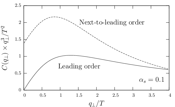
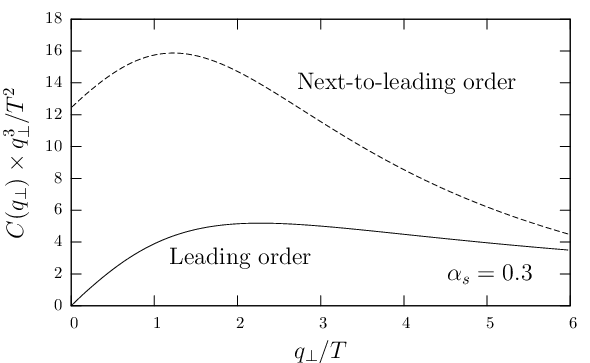
The ${\cal O}(g)$ corrections to $C(q_{\perp})$, which being due to $gT$-scale physics only arise for $q_{\perp}\sim gT\ll T$, are illustrated in fig. 1. Both the LO and NLO kernels $C(q_{\perp})$ are proportional to the (quadratic) Casimir of the gauge group representation of the jet. The “leading order curves” is based on the full (unscreened) expression (22) at hard momenta, multiplied by $q_{\perp}^{2}/(q_{\perp}^{2}{+}m_{D}^{2})$ to make it merge smoothly with the analytic result (10) at low momenta, following the prescription given in [26]. The “next-to-leading order” curves use the leading order curves plus $C(q_{\perp})^{(\rm NLO)}$ given in (20).

The NLO correction is already quite large for $\alpha_{s}=0.1$, giving nearly a factor of 2 around $q_{\perp}\approx T$. As discussed in the Introduction, this is consistent with the behavior observed for ${\cal O}(g)$ effects in other quantities. At $\alpha_{s}=0.3$, a typical value used in comparisons with RHIC data (see e.g. [27]), it is clear that the strength of the correction has grown out of control, meaning that (presently unknown) yet higher-order corrections are most certainly also important (though our results suggest that the value of $\alpha_{s}$ needed to fit the data might be significantly smaller than the estimate of [27]).

An interesting by-product of the approach used in this paper is that it extends naturally to higher orders: it makes perfect sense to evaluate the gauge-invariant Wilson loop (9) nonperturbatively within the Euclidean three-dimensional EQCD theory, for instance using the lattice. Although this may not include all ${\cal O}(g^{2})$ corrections to $C(q_{\perp})$ (contributions from the hard scale $2\pi T$ will be missed), by analogy with the works on the pressure discussed in the Introduction, these missing contributions can be expected to be numerically suppressed¹¹ 1 Their description could turn out be very complicated, though, because jet evolution at ${\cal O}(g^{2})$ should contain, among other things, the analog of the NLO vacuum DGLAP splitting amplitudes in the presence of the LPM effect (described below). Also, various effects involving the scale evolution of the medium constituents and coupling constant evolution should arise. . We leave to future work the study of this interesting possibility.

The dominant energy loss mechanism of high energy particles (at weak coupling) is bremsstrahlung (including quark-antiquark pair production), triggered by soft collisions against plasma constituents. The theoretical description of these processes, at the leading order in the coupling, is well-established [28] [29] [30]. Their duration $t_{\rm form}$ depends on the energy of the participants, and can interpolate between the Bethe-Heitler (single scattering) regime $t_{\rm form}\sim E/q_{\perp}^{2}\sim E/m_{D}^{2}$ at energies $E\stackrel{{\scriptstyle<}}{{{}_{\sim}}}T$, and the Landau-Pomeranchuk-Migdal (LPM) [31] (multiple-scattering) regime at high energies $E\gg T$, with $t_{\rm form}\sim\sqrt{E/\hat{q}}$, in which destructive interference between different collisions plays a significant role.

In all of these regimes, however, the description factors into a “hard” collinear splitting vertex (Dokshitzer-Gribov-Lipatov-Altarelli-Parisi, DGLAP vertex [33]), times an amplitude (wavefunction in the transverse plane) which describes the in-medium evolution of the vertex. The latter accounts for the collisions which trigger, and occur during, the splitting process [28] [29] [30]. The DGLAP vertices themselves only involves hard scale physics (in essence, they are Clebsch-Gordon coefficients between states of different helicities) and thus cannot receive ${\cal O}(g)$ corrections; the NLO effects, which come from soft classical fields with $p\sim gT$, are included in their dressing amplitude.

In section 6 we discuss these amplitudes at NLO and show that the relevant (three-body) collision kernel factors as a sum of two-body kernels $C(q_{\perp})$, exactly like the LO one does [28] [29] [30, 32]. As a consequence, our results can be used to give a full NLO treatment of radiative jet energy loss; one must simply include the NLO shift (20) to the two-body kernel $C(q_{\perp})$ which serves as an input to these calculations²² 2 For instance, one would simply modify “$C(q_{\perp})$” in [32], which is actually equal to $C(q_{\perp})/(g^{2}C_{s}T)$ in our conventions. .

When the effects of a large number of small collisions are added together, it is natural to replace them by an effective diffusive process. The diffusion coefficient relevant for transverse momentum broadening, $\hat{q}$, is defined as the second moment of the collision kernel (1):

The ultraviolet cutoff $|q_{\perp}|<q_{\rm max}$ is needed to deal with the weak power-law falloff $C(q_{\perp})\sim g^{4}T^{3}/q_{\perp}^{4}$ at large $q_{\perp}$, which leads to a logarithmic dependence of $\hat{q}$ on $q_{\rm max}$. This is a leading order logarithm; below we shall comment on the value of the cutoff $q_{\rm max}$. Using our NLO kernel (20) we can calculate the expansion of $\hat{q}$ up to terms of order $g^{2}$ ³³ 3 Version 1 of the present paper contained a transcription error which is now corrected in (3). The argument of the logarithm (incorrectly) read $q^{*}$ as opposed to $m_{D}$ obtained from (23) and (24).:

with $\xi^{(\rm NLO)}=\frac{3}{16\pi}\left(3\pi^{2}+10-4\log 2\right)\simeq 2.1985$ a constant calculated in section 5, characterizing the NLO correction to $\hat{q}$, and $m_{D}^{2}=g^{2}T^{2}(N_{c}+N_{f}T_{f})/3$ the leading-order Debye mass. In QCD with $N_{f}=3$ flavors of fundamental quarks, $C_{A}=3$ and $N_{f}T_{f}=1.5$. For a discussion of the leading order result and logarithms, we refer the reader to P. Arnold’s work [26], from which the high-precision numbers were taken.

The series (3) is meant to represent the expansion in $g$ of the area under the curve of plots such as fig. 1. For $\alpha_{s}=0.1$ and a quark ($C_{s}=\frac{4}{3}$) the area under the leading order curve in the figure (up to $q_{\rm max}=4T$) would yield $\hat{q}^{\rm LO}\approx 2.60~(\mbox{T/GeV})^{3}\,{\rm GeV^{2}/fm}$ whereas the first two lines of (3) give $\hat{q}^{\rm LO,th}\approx 2.08~(\mbox{T/GeV})^{3}\,{\rm GeV^{2}/fm}$. The NLO shift is $\Delta\hat{q}\approx 2.22~(\mbox{T/GeV})^{3}\,{\rm GeV^{2}/fm}$ from the figure, about a factor of two effect, and $\Delta\hat{q}^{\rm th}\approx 5.26~(\mbox{T/GeV})^{3}\,{\rm GeV^{2}/fm}$ according to (3). Thus the third line of (3) itself suffers from sizeable truncation errors compared to our full NLO result (20). We would like to stress, however, that (20), and fig. 1, is not merely a simple truncation error from a lower-order contribution but represents a genuine NLO effects.

As discussed in the preceding subsection, it would be premature to attempt comparison of our $\hat{q}$ results with experimental data, since it is clear that (yet unknown) higher-order corrections should also be important at physically relevant couplings. It is also worth noting that different approximation schemes taking $\hat{q}$ as input (this excludes the AMY scheme [30, 32], which uses the full $C(q_{\perp})$) when fitted to RHIC data, tend to disagree rather significantly on its preferred value [3]; since a critical analysis of these approximations lies beyond our scope, this simply means it is not completely clear which experimentally-extracted value of $\hat{q}$ we should comparing with.

It seems appropriate here to recall some subtleties associated with the phenomenological parameter $\hat{q}$, which do not arise if one instead works with the full collision kernel $C(q_{\perp})$. First, the value of the cutoff $q_{\rm max}$ to be used in (3) is process-dependent: since the $q_{\perp}{>}q_{\rm max}$ tail of $C(q_{\perp})$ describes collisions occurring on a finite rate⁴⁴ 4 I am indebted to G. D. Moore for this discussion. $\Gamma_{(q_{\perp}>q_{\rm max})}\sim g^{4}T^{3}/q_{\rm max}^{2}$, weighting them with $q_{\perp}^{2}$ in (23) ceases to make sense for $\Gamma_{(q_{\perp}>q_{\rm max})}^{-1}\stackrel{{\scriptstyle>}}{{{}_{\sim}}}t_{\rm jet}$, with $t_{\rm jet}$ the jet’s lifetime, to be replaced with a formation time $t_{\rm form}$ for bremsstrahlung pairs in the context of energy loss calculations. Therefore, parametrically, one should set $q_{\rm max}\sim\sqrt{g^{4}T^{3}t_{\rm jet}}$. For bremsstrahlung in the deep LPM regime, $t_{\rm jet}\to t_{\rm form}\sim\sqrt{E/\hat{q}}$ so $q_{\rm max}\sim g(ET^{3})^{1/4}$ [34]⁵⁵ 5 This should be contrasted with the often-used kinematic cutoff $q_{\rm max}^{2}\approx ET$. .

Second, the presence of the ultraviolet tail implies that collisions having $q_{\perp}\sim q_{\rm max}$ (with $q_{\rm max}$ the physical cutoff as determined above), which are intrinsically non-diffusive, already contribute at the next-to-leading logarithm order to bremsstrahlung rates. That is, they contribute at ${\cal O}(1)$ compared to the log-enhanced diffusive contribution $\sim\log q_{\rm max}/m_{D}$ coming from $m_{D}\ll q_{\perp}\ll q_{\rm max}$. Therefore, approximations based on diffusive physics lead, at best, to expansions in inverse logarithms of the energy. Such expansions were systematically studied in [34], with the conclusion that formulae to next-to-leading logarithm can be trusted at least when $E_{\rm jet}\stackrel{{\scriptstyle>}}{{{}_{\sim}}}10T$, with the inclusion of the subleading term (e.g. the constant under the logarithm) being mandatory. None of the presently applied approaches which rely on $\hat{q}$ as a phenomenological parameter presently includes such subleading logarithms (see [3, 35] and references therein for an overview of these approaches).

Field operators at space-like separated points (anti)commute with each other and their correlator does not depend on the operator ordering. For two-point functions at vanishing time separation, a well-known Euclidean representation holds [36]:

with the sum running over the Matsubara frequencies $\omega_{n}=2\pi inT$, $\beta=1/T$, and with $G^{E}_{ij}$ the Euclidean correlator of some operators ${\cal O}_{i,j}$ taken here to be bosonic.

In Lorentz-covariant theories, (4) can be extended immediately to any correlator which is equal-time in a suitable boosted frame. Specifically, under a $z$-axis boost with velocity $\tilde{v}$, the thermal density matrix transforms to:

the primed quantities referring to quantities in the boosted frame; $\tilde{\gamma}=\frac{1}{\sqrt{1{-}\tilde{v}^{2}}}$. The identification of $H^{\prime}$ and $P^{\prime}{}^{3}$ as the generators of time and space translation shows periodic identification $x^{\prime}{}^{\mu}=x^{\prime}{}^{\mu}+i\tilde{\gamma}(\beta,-\tilde{v}\beta,0_{\perp})$ for the geometry associated to (5), with associated quantization condition on the “Matsubara frequencies” $p^{\prime}{}^{0}+\tilde{v}p^{\prime}{}^{3}=2\pi inT/\tilde{\gamma}$. The spatial momentum $p^{\prime}{}^{3}$ must be kept real: it serves as a label for the physical states living on the $x^{\prime}{}^{0}=0$ hyperplane. Thus only the frequency $p^{\prime}{}^{0}$ is complex. This determines the extension of (4) to equal-time two-point functions in the boosted frame:

It will be convenient to boost this formula back to the plasma rest frame, and to write it for general space-time arguments ($\tilde{v}=\frac{x^{0}}{x^{3}}$):

Eq. (7) is the main result of this section. It differs from (4) only due to the imaginary part of $p^{3}_{n}$, which, in fact, is required for the convergence of the sum over $n$: it prevents the Fourier exponential to contain exponentially growing terms as opposed to pure phases. Eq. (7) extends in a straightforward way to any higher-point correlator supported on $(\frac{x^{0}}{x^{3}}=\tilde{v})$-type hyperplanes: one gets a summation-integration $\sum_{n}\int_{p}$, with the $p_{n}$ as in (7), for all external legs, subject to the usual restriction of momentum conservation (and thus of “$n$ conservation”), as for equal-time higher-point correlators [36]. The momenta running in loops must also be “twisted” like those in (7), e.g. ${\rm Im}\,p^{3}=\tilde{v}{\rm Im}\,p^{0}$, to reflect the boosted-frame origin of the formula⁶⁶ 6 Note that this gives an implicit dependence on the velocity $v$ to $G^{E}_{ij}(p_{n}^{0},p^{3}_{n},p_{\perp})$ appearing in (7). . This ensures that the imaginary part of every momentum is time-like, which is the natural domain of Euclidean physics.

We will be interested in the amplitudes of ultrarelativistic dipoles moving with velocity $v=1$, e.g. $x^{3}=x^{0}$ (note $\tilde{v}=1/v$ in general). Our derivation of (7) might seem compromised, since an “infinite” boost with velocity $\tilde{v}=1$ obviously doesn’t exist. However, a more careful look at the argument reveals that the boost plays no important role: after all we un-did it in the end. All that is really important, is that we can imagine quantizing the system along hyperplanes parallel to $\tilde{v}$, and express the thermal density matrix within these hyperplanes. Since it is certainly possible to quantize a system along light fronts, the result (7) must hold for $x^{3}=x^{0}$. An alternative derivation of this, based on sum rules, is also given in App. A.

The attentive reader might complain that setting $x^{3}=x^{0}$ in (7) corresponds to taking a $v\searrow 1$ limit, whereas the physically relevant regime $v\nearrow 1$ lies beyond the reach of (7). Are we claiming that these limits are equivalent in general? No⁷⁷ 7 In strongly coupled theories accessible to gauge-string duality, these two limits are known to be physically distinct. A calculation of $\hat{q}$ for a physical massive quark moving with $v<1$ (in the sense of its momentum broadening coefficient) by Teaney and Casalderrey-Solana [21], and by Gubser [22], found a divergence $\hat{q}\sim(1-v^{2})^{-1/4}\sqrt{\lambda}T^{3}$ as $v\nearrow 1$. This calculation is valid for energies $E<M^{3}/\lambda T^{2}$, beyond which the coherence time of the force acting on the quark becomes of order the time scale of Langevin dynamics [22]; a time-independent description is then impossible. This suggests that $\hat{q}$ for $v<1$ should depend on a cutoff time scale, as is the case at weak coupling. On the other hand, the $v\searrow 1$ limit has been studied by Rajagopal, Liu and Wiedemann [19, 20], by embedding Euclidean worldsheets into ${\rm AdS}_{5}$ space, and no divergences were met in this limit. It is thus qualitatively quite distinct. . Our claim, explained in the introduction, is merely that for classical plasma physics effects they are equivalent — to the extent that the observable of interest is only passively probing a soft classical background, only a phase-space suppressed fraction of which propagates collinearly with the jet, this seems to be rather robust. It is unclear whether this will remain true when quantum effects are included (which will enter at $\sim g^{2}$), though, because of collinear components present in the jet’s own wavefunction.

Naturally, the contribution from soft physics (momenta $\sim gT$) to sums like (7) is expected to be dominated by the $n=0$ mode. We will thus begin by “integrating out” the modes with $n\neq 0$.

First we claim that loop diagrams for which all external momenta have $n=0$ are equal to the standard ones. These two sets of diagrams have $p^{0}=0$ and $p_{z}$ real, and could only differ due to the “twisted” Matsubara momenta (7) which circulate in the former; our claim is that this does not affect their value. The reason is that the imaginary part of every momentum $P$ in such loops is time-like with a real part obeying ${\rm Re}\,p^{0}=0$, ensuring that ${\rm Re}\,P^{2}$ is positive-definite. The imaginary part of the $p^{3}$ integration contours can thus be deformed from ${\rm Im}\,p^{3}=\tilde{v}{\rm Im}\,p^{0}$ to ${\rm Im}\,p^{3}=0$, without crossing any pole.

In particular, the modes with $n=0$ are described by precisely the standard “electric QCD” (EQCD) three-dimensional effective theory [37, 38]. EQCD is pure three-dimensional Yang-Mills with coupling constant $g^{2}_{3}=g^{2}T$ coupled to a massive adjoint scalar $A_{0}$ of mass $m_{D}$. It is an effective theory for the $gT$ scale (the Euclidean version of the hard thermal loop theory [14]), in which the loop expansion proceeds in powers of $g^{2}T/m_{D}\sim g$. Its parameters do not receive ${\cal O}(g)$ corrections.

The propagators of EQCD are:

(We use the tilde to denote that these are three-dimensional propagators.) The minus sign in front of the $A^{0}$ propagator reflects the fact that we will couple it to Minkowski-space Wilson lines: we have not performed a Wick rotation.

In addition to its interaction with the $n=0$ modes, we must also include the direct coupling of the operator of interest to the $n\neq 0$ modes. Physically, and as shown in Appendix A, a contribution from these modes would correspond, in the real-time formalism, to a failure of the soft approximation $n_{B}(p^{0})\approx T/p^{0}$. Such a failure would signal a contribution from the $p^{0}\sim T$ region in Minkowski space, which would necessary be signaled by ultraviolet divergences in the soft approximation, since this approximation correctly describes the intermediate region $gT\ll p^{0}\ll T$ and any contribution from the scale $T$ should leave an imprint on this region. Thus, provided we do not find ultraviolet divergences from the $n=0$ contribution alone (which computes exactly the soft approximation, see Appendix  A), this argument shows that we can safely ignore the direct coupling to the $n\neq 0$ modes. This will turn out to be our case.

The evolution of the transverse momentum of a high-energy particle can be described by looking at its density matrix, as described in detail in [21]. For classical effects, however (and even more so because we are taking the velocity to be $v=1{+}\epsilon$), we can neglect operator ordering issues and replace the evolution of the density matrix by that of a dipole; we will come back to operator ordering issues in section 6.2.

High energy dipoles ($E\gg m_{D}$) propagate eikonally in the soft classical background. The collision kernel describing the evolution of its transverse momentum can thus be recovered from the Fourier transform of the (long-time limit of the) dipole propagation amplitude $W$ [28] [29] [39]:

$C(q_{\perp})$ is short for $(2\pi)^{2}d\Gamma/d^{2}q_{\perp}$, as in (1). The dipole amplitude $W(t,x_{\perp})$ is given by the trace of a long, thin rectangular Wilson loop stretching along the light-cone coordinate $x^{+}$, with a small transverse extension $x_{\perp}$ (see fig. 2).

The naive dimensional reduction of the Wilson loop (9) yields a Wilson loop stretching along the $z$-axis of the three-dimensional EQCD theory. It couples to the linear combination $A_{+}\equiv(A_{z}+A_{0})$ of the EQCD fields, reflecting its ultrarelativistic origin. This “naive” dimensional reduction corresponds to keeping only the direct coupling to the $n=0$ modes. As explained in subsection 3.2, this will be justified provided we do not find ultraviolet divergences.

At the lowest order in perturbation theory, only the single-gluon exchange diagram ((a) of fig. 3) contributes,

where we have used (8). The compact form (10) was first obtained by means of sum rules by Aurenche, Gelis and Zaraket [18], which we show in Appendix A are equivalent to our approach.

At the next-to-leading order (one-loop), self-energy insertions to the single-gluon diagram (b) contribute (we will often write “$q_{\perp}$” for a three-vector with $q_{z}=0$, which should cause no confusion; “$\int_{p}$” is short for $\int\frac{d^{3}p}{(2\pi)^{3}}$):

Each bracket includes the contributions of one fish and one tadpole diagram, while the last one also includes the ghost loop.

The (linear) ultraviolet divergences in (11) are to be canceled by matching counter-terms that can be unambiguously calculated within the framework of dimensional reduction [37, 38]. They merely represent the (hard thermal loop) coupling of the $n\neq 0$ gluons to the soft $n=0$ ones, e.g. the gluon contribution to the $A^{0}$ mass squared $m_{D}^{2}$. The fact that the direct coupling to exchange gluons with $q^{0}=q^{3}\neq 0$ does not contribute to the divergences can also be checked explicitly, from the convergence, with respect to $q^{3}$, of the real-time integral (22) (this justifies making the soft approximation on $q^{0}$). Thus the divergences in (11) do not signal the presence of “new contributions” beyond the EQCD effective theory, as discussed in section 3.2.

Employing dimensional regularization, the divergences simply go away⁸⁸ 8 The dimensionally-regulated integrals (11) have poles in dimensions 2 and 4 but are finite and unambiguous in dimension 3. and the counter-terms are zero to ${\cal O}(g)$ [38]. This way we obtain (all our arctangents run from $0$ to $\pi/2$):

Diagram (c) plus its permutation contribute:

In the Feynman gauge, there is no contribution involving only transverse gauge fields: such a contribution would involve the (trivial) $zzz$ vertex. Eq. (13) is manifestly convergent.

Our calculation is based on a quasiparticle expansion, e.g. we simply set on-shell the external legs of scattering diagrams. The relevant expansion parameter is $g$, e.g. the ratio of the scattering width $\sim g^{2}T$ to the scattering’s natural frequency scale $m_{D}$. Thus in evaluating the external state corrections (d) we need only keep those effects which are not suppressed by the smallness of the width. A narrow resonance being described by just its position and the total area under it, this means that diagram (d), at ${\cal O}(g)$, produces only mass-shell corrections and wave-function renormalization factors. The (here imaginary) “mass-shell” corrections have no effects: they are identical for the initial and final states, so the “energy” (read $z$-momentum) transfer is zero in any case. The wave-function renormalization contribution is given by an energy derivative of the eikonal self-energy, and (e) is unambiguous, yielding respectively (including all diagrams of similar topology):

The sum of (d) and (e) is proportional to $C_{A}$ and identically vanishes in the abelian theory ($C_{A}=0$), as required by abelian exponentiation⁹⁹ 9 Abelian Wilson loops, computed using Gaussian distribution for gauge fields (as is done by diagrams (d)-(g), for which only the two-point function of the gauge field enters), simply exponentiate: $\langle e^{\int A}\rangle=\exp(\frac{1}{2}\langle\int A\int A\rangle)$. As a consequence, the collision kernel as defined from (9) is tree-level exact in such theories; there is no interference between scattering events. .

Part of diagram (f) is already included by the exponentiation of (10) (diagram (a)): this generates the approximation to (f) in which the intermediate eikonal propagators are put on-shell. To avoid double-counting, this must be subtracted. We must first regulate the associated “pinching” ($q_{z}\to 0$) singularity, which we do by flowing a small external $z$-momentum $\omega$ into the Wilson loop. We then take the limit $\omega\to 0$ after the subtraction. Diagram (g) poses no difficulty.

Eq. (16) has a well-defined $\omega\to 0$ limit, as follows from the identity $1/(p_{z}{+}i\epsilon-1/(p_{z}{-}i\epsilon)=-2\pi i\delta(p_{z})$. This limit takes a form identical to (17) and the sum is proportional to $C_{A}$, again as required by abelian exponentiation. This confirms the correctness of our evaluation of (f).

The sum of diagrams (d)-(g) yields:

The function $\tilde{G}_{++}$ is $\tilde{G}_{00}+\tilde{G}_{zz}$, as given in eq. (8). To evaluate (18) we have found convenient to first apply integration by parts to the $1/(p_{z}-i\epsilon)^{2}$ denominator, which removes the explicit $p_{z}$-dependence and reduces the integral to a set of standard isotropic Feynman integrals. Eq. (18) is manifestly infrared- (and ultraviolet-) safe, upon enforcing $p\leftrightarrow(q_{\perp}{-}p)$ symmetry.

In summary, we have obtained all ${\cal O}(g)$ contributions to the collision kernel $C(q_{\perp})$:

These expressions are valid for $q_{\perp}\ll T$. The leading order kernel for $q_{\perp}\stackrel{{\scriptstyle>}}{{{}_{\sim}}}T$ gets slightly modified, see (22).

The reader might wonder as to the appearance of arctangents with two distinct arguments in (20). They can be understood by looking in the complex $q_{\perp}^{2}$-plane: $\tan^{-1}(q_{\perp}/2m_{D})$ has a branch cut starting at $q_{\perp}^{2}=-4m_{D}^{2}$, exhibiting its origin from the exchange of a pair of two quanta of mass $m_{D}$ (longitudinal gluons). The branch cut of $\tan^{-1}(q_{\perp}/m_{D})$, starting at $q_{\perp}^{2}=-m_{D}^{2}$, arises from the exchange of one longitudinal and one transverse gluon. Both arctangents occur, since both of these pairs of states can be exchanged. Exchange of two massless quanta also occurs, and generates $1/\sqrt{q_{\perp}^{2}}$-type of discontinuities instead of arctangents.

References

- [1] K. Adcox et al. [PHENIX Collaboration] Phys. Rev. Lett. 88 022301 (2003).
- [2] C. Adler et al. [STAR Collaboration] Phys. Rev. Lett. 89 202301 (2002).
- [3] S. A. Bass, C. Gale, A. Majumder, C. Nonaka, G. Y. Qin, T. Renk and J. Ruppert, arXiv:0808.0908 [nucl-th].
- [4] P. Arnold and C. x. Zhai, Phys. Rev. D 51, 1906 (1995) [arXiv:hep-ph/9410360].
- [5] E. Braaten and A. Nieto, Phys. Rev. Lett. 76, 1417 (1996) [arXiv:hep-ph/9508406].
- [6] K. Kajantie, M. Laine, K. Rummukainen and Y. Schroder, Phys. Rev. D 67, 105008 (2003) [arXiv:hep-ph/0211321]; F. Di Renzo, M. Laine, V. Miccio, Y. Schroder and C. Torrero, JHEP 0607, 026 (2006) [arXiv:hep-ph/0605042].
- [7] H. Schulz, Nucl. Phys. B 413 353 (1993)
- [8] M. E. Carrington, A. Gynther and D. Pickering, Phys. Rev. D 78, 045018 (2008) [arXiv:0805.0170 [hep-ph]].
- [9] J. P. Blaizot, E. Iancu and A. Rebhan, Phys. Rev. D 63, 065003 (2001) [arXiv:hep-ph/0005003].
- [10] S. Caron-Huot and G. D. Moore, Phys. Rev. Lett. 100, 052301 (2008) [arXiv:0708.4232 [hep-ph]]; S. Caron-Huot and G. D. Moore, JHEP 0802, 081 (2008) [arXiv:0801.2173 [hep-ph]].
- [11] M. Laine and Y. Schroder, JHEP 0503, 067 (2005) [arXiv:hep-ph/0503061].
- [12] J. P. Blaizot, E. Iancu and A. Rebhan, Phys. Rev. D 68, 025011 (2003) [arXiv:hep-ph/0303045].
- [13] K. Kajantie, M. Laine, K. Rummukainen and Y. Schroder, Phys. Rev. Lett. 86, 10 (2001) [arXiv:hep-ph/0007109].
- [14] E. Braaten and R. D. Pisarski, Nucl. Phys. B 337, 569 (1990); J. Frenkel and J. C. Taylor, Nucl. Phys. B 334, 199 (1990).
- [15] J. P. Blaizot and E. Iancu, Phys. Rept. 359, 355 (2002) [arXiv:hep-ph/0101103].
- [16] P. F. Kelly, Q. Liu, C. Lucchesi and C. Manuel, Phys. Rev. D 50, 4209 (1994)
- [17] E. Braaten and M. H. Thoma, Phys. Rev. D 44, 2625 (1991); Phys. Rev. D 44, 1298 (1991).
- [18] P. Aurenche, F. Gelis and H. Zaraket, JHEP 0205, 043 (2002) [arXiv:hep-ph/0204146].
- [19] H. Liu, K. Rajagopal and U. A. Wiedemann, Phys. Rev. Lett. 97, 182301 (2006) [arXiv:hep-ph/0605178].
- [20] H. Liu, K. Rajagopal and Y. Shi, JHEP 0808, 048 (2008) [arXiv:0803.3214 [hep-ph]].
- [21] J. Casalderrey-Solana and D. Teaney, JHEP 0704, 039 (2007) [arXiv:hep-th/0701123].
- [22] S. S. Gubser, Nucl. Phys. B 790, 175 (2008) [arXiv:hep-th/0612143].
- [23] Y. Hatta, E. Iancu and A. H. Mueller, JHEP 0805, 037 (2008) [arXiv:0803.2481 [hep-th]].
- [24] S. S. Gubser, D. R. Gulotta, S. S. Pufu and F. D. Rocha, arXiv:0803.1470 [hep-th].
- [25] P. M. Chesler, K. Jensen, A. Karch and L. G. Yaffe, arXiv:0810.1985 [hep-th].
- [26] P. Arnold and W. Xiao, arXiv:0810.1026 [hep-ph].
- [27] G. Y. Qin, J. Ruppert, C. Gale, S. Jeon, G. D. Moore and M. G. Mustafa, Phys. Rev. Lett. 100, 072301 (2008) [arXiv:0710.0605 [hep-ph]].
- [28] R. Baier, Y. L. Dokshitzer, S. Peigne and D. Schiff, Phys. Lett. B 345, 277 (1995) [arXiv:hep-ph/9411409]. R. Baier, Y. L. Dokshitzer, A. H. Mueller, S. Peigne and D. Schiff, Nucl. Phys. B 483, 291 (1997) [arXiv:hep-ph/9607355].
- [29] B. G. Zakharov, JETP Lett. 65, 615 (1997) [hep-ph/9704255]; 63 952 (1996) [hep-ph/9607440].
- [30] P. Arnold, G. D. Moore and L. G. Yaffe, JHEP 0206, 030 (2002) [arXiv:hep-ph/0204343].
- [31] L. D. Landau and I. Pomeranchuk, Dokl. Akad. Nauk Ser. Fiz. 92 (1953) 535; L. D. Landau and I. Pomeranchuk, Dokl. Akad. Nauk Ser. Fiz. 92 (1953) 735; A. B. Migdal, Dokl. Akad. Nauk S.S.S.R. 105, 77 (1955); A. B. Migdal, Phys. Rev. 103, 1811 (1956).
- [32] S. Jeon and G. D. Moore, Phys. Rev. C 71, 034901 (2005) [arXiv:hep-ph/0309332].
- [33] V. N. Gribov and L. N. Lipatov, Sov. J. Nucl. Phys. 15 (1972) 438; V. N. Gribov and L. N. Lipatov, Sov. J. Nucl. Phys. 15 (1972) 675; L. N. Lipatov, Sov. J. Nucl. Phys. 20 (1975) 94; G. Altarelli and G. Parisi, Nucl. Phys. B126 (1977) 298; Yu. L. Dokshitzer, Sov. Phys. JETP 46 (1977) 641.
- [34] P. Arnold and C. Dogan, arXiv:0804.3359 [hep-ph].
- [35] A. Majumder, arXiv:0810.1367 [nucl-th].
- [36] J. I. Kapusta and C. Gale, Cambridge, UK: Univ. Pr. (2006) 428 p.
- [37] T. Appelquist and R. D. Pisarski, Phys. Rev. D 23, 2305 (1981).
- [38] K. Farakos, K. Kajantie, K. Rummukainen and M. E. Shaposhnikov, Nucl. Phys. B 425, 67 (1994) [hep-ph/9404201].
- [39] Z. t. Liang, X. N. Wang and J. Zhou, Phys. Rev. D 77, 125010 (2008) [arXiv:0801.0434 [hep-ph]].
- [40] L. S. Brown, Phys. Rev. D 62, 045026 (2000) [arXiv:physics/9911056].
- [41] J. Schwinger, J. Math. Phys. 2, 407 (1961), L. V. Keldysh, Sov. Phys. JETP 20, 1018 (1964).