跳到论文正文
W Papers独立论文阅读器 arXiv:0811.1460 论文正文 计算阅读时间 · 0%
引用这篇论文根据当前论文元数据生成,正式投稿前建议核对。


License: arXiv.org perpetual non-exclusive license
arXiv:0811.1460v1 [physics.atom-ph] 10 Nov 2008

Parity Violation in Hydrogen
and Longitudinal Atomic Beam Spin Echo I

Timo Bergmann1, ††thanks: Timo.Bergmann@web.DE††thanks: present address: SAP AG, Walldorf    Maarten DeKieviet2, ††thanks: maarten@physi.Uni-Heidelberg.DE    Thomas Gasenzer1, ††thanks: T.Gasenzer@ThPhys.Uni-Heidelberg.DE    Otto Nachtmann1, ††thanks: O.Nachtmann@ThPhys.Uni-Heidelberg.DE    Martin-I. Trappe1, ††thanks: M.Trappe@ThPhys.Uni-Heidelberg.DE Affiliation: Institut für Theoretische Physik, Universität Heidelberg,
Philosophenweg 16, 69120 Heidelberg, Germany
Affiliation: Physikalisches Institut, Universität Heidelberg,
Philosophenweg 12, 69120 Heidelberg, Germany
Received: August 24, 2026
Abstract

We discuss the propagation of hydrogen atoms in static electric and magnetic fields in a longitudinal atomic beam spin echo (lABSE) apparatus. There the atoms acquire geometric (Berry) phases that exhibit a new manifestation of parity-(P-)violation in atomic physics. We provide analytical as well as numerical calculations of the behaviour of the metastable 2S states of hydrogen. The conditions for electromagnetic field configurations that allow for adiabatic evolution of the relevant atomic states are investigated. Our results provide the theoretical basis for the discussion of possible measurements of P-violating geometric phases in lABSE experiments.
HD–THEP–08–19

pacs
03.65.VfPhases: geometric; dynamic or topological and 11.30.ErCharge conjugation, parity, time reversal, and other discrete symmetries and 31.70.HqTime-dependent phenomena: excitation and relaxation processes, and reaction rates and 32.80.YsWeak-interaction effects in atoms

1 Introduction

In this paper we continue our theoretical studies towards the realisation of an experiment to measure P-violating effects using the methods available with an atomic beam interferometer as described in [1]. Starting with the paper [2] many theoretical and experimental studies of P-violation due to neutral current exchange were made for heavy atoms. For reviews see [3, 4]. The most precise results so far are from experiments with Cs [5, 6]. The experimental observation of P-violation in the lightest atoms, hydrogen (H) and deuterium (D), still is an open problem [7]. For the early experimental efforts in this direction see [8, 9, 10]. In [11, 12] we have studied parity violating geometric phases. These are interesting quantum mechanical phenomena by themselves and we think it is worthwhile to try measuring them. In the present paper we shall develop the necessary theoretical tools for a description of the behaviour of an atom in the interferometer described in [1]. The aim is to calculate the relevant phases which atoms pick up when travelling through the interferometer and to construct observables sensitive to P-violating geometric phases. We shall focus on the hydrogen states with principal quantum number n=2n=2, in particular on the metastable 2S states. Our paper is organised as follows. In Section 2 we set up the basic equations governing the motion of the atom in the n=2n=2 states as it travels through the interferometer. In Section 3 we study the equation for a single substate. Section 4 deals with two metastable 2S states and with their interference effects. In Section 5 we draw our conclusions. A concrete proposal for a measurement of P-violating geometric phases will be given in a follow up paper. Our notation is explained in Appendix A which collects also many useful formulae. Furthermore, we discuss in Appendix A the conditions for adiabatic evolution of the atomic states for the case considered. Appendix B contains the details of our calculations concerning the motion of a single 2S state in the interferometer. In Appendix C we discuss in detail the interference effects of two states. Throughout our work we use natural units ℏ=c=1\hbar=c=1 if not indicated otherwise.

2 A hydrogen atom in the interferometer

We consider in this section the case of a hydrogen atom being in a superposition of n=2n=2 internal states and travelling through an interferometer of the type presented in [1]. The latter is, for a theorist, a device producing static electric and magnetic fields acting on the atom. Schematically this is shown in Figure 1.

Refer to caption
Figure 1: Schematic view of the longitudinal spin echo interferometer. The coordinate system used is indicated. The coordinate along the beam direction is denoted by zz. The atom is prepared in a wave packet around z0z_{0} and analysed around zaz_{a}. In the example discussed in Section 4 we start with a superposition |ψ⁡(z0)⟩|\psi(z_{0})\rangle of two states, labeled with |9)|9) and |11)|11). After passing the magnetic and electric fields 𝓑⁡(z)\bm{\mathcal{B}}(z) and 𝓔⁡(z)\bm{\mathcal{E}}(z) the wavefunction is projected onto an analysing state |ψ⁡(za)⟩|\psi(z_{a})\rangle, for example again onto a superposition of the states |9)|9) and |11)|11).

The magnetic field strength 𝓑\bm{\mathcal{B}} and the electric field strength 𝓔\bm{\mathcal{E}} are supposed to depend only on the zz coordinate and to be nonzero only between z0z_{0} and zaz_{a}. Here z0z_{0} marks the place at the beginning of the interferometer around which, in a field-free region, the wave packet of the atom is prepared. Similarly, zaz_{a} at the end of the interferometer marks the place where, again in a field-free region, the internal state of the atom is analysed.

The hydrogen atom in a superposition of states with principal quantum number n=2n=2 is described by a 16-component spinor

|ψ(𝐱,t)⟩=∑α=116fα(𝐱,t)|α;0).\displaystyle|\psi(\mathbf{x},t)\rangle=\sum^{16}_{\alpha=1}f_{\alpha}(\mathbf{x},t)|\alpha;0)\ . (1)

Here |α;0)|\alpha;0), α=1,…,16\alpha=1,\dots,16, are the basis states for 𝓑=0\bm{\mathcal{B}}=0 and 𝓔=0\bm{\mathcal{E}}=0, that is the 2S1/2, 2P1/2 and 2P3/2 states with the numbering as given in Table 2 of Appendix A. The Schrödinger equation describing the undecayed n=2n=2 states reads

i​∂∂t​|ψ⁡(𝐱,t)⟩=[−12​m​Δ+ℳ¯​(z)+E0]​|ψ⁡(𝐱,t)⟩.\displaystyle\mathrm{i}\frac{\partial}{\partial t}|\psi(\mathbf{x},t)\rangle=\left[-\frac{1}{2m}\Delta+{\underline{\mathscr{M}}}(z)+E_{0}\right]|\psi(\mathbf{x},t)\rangle\ . (2)

Here mm is the atom’s mass and ℳ¯​(z)\underline{\mathscr{M}}(z) is the non-hermitian energy or mass matrix as described in Section of [12]. There the center of the real parts of the energy levels of the free 2P1/2 states was chosen as the (arbitrary) zero for the energy scale. In the following it is convenient to choose this zero point of the energy differently. Therefore, we introduce in (2) a real constant E0E_{0} which we can choose freely. The mass matrix ℳ¯​(z)\underline{\mathscr{M}}(z) is given by

ℳ¯​(z)\displaystyle\underline{\mathscr{M}}(z) =ℳ¯~0​(δ1,δ2)−𝑫¯⋅𝓔⁡(z)−𝝁¯⋅𝓑⁡(z),\displaystyle=\underline{\mathscr{\tilde{M}}}_{0}(\delta_{1},\delta_{2})-{\underline{\bm{D}}}\cdot{\bm{\mathcal{E}}}(z)-\underline{\bm{\mu}}\cdot{\bm{\mathcal{B}}}(z)\ , (3)
ℳ¯~0​(δ1,δ2)\displaystyle\underline{\mathscr{\tilde{M}}}_{0}(\delta_{1},\delta_{2}) =ℳ¯0+δ1​ℳ¯P​V(1)+δ2​ℳ¯P​V(2).\displaystyle=\underline{\mathscr{M}}_{0}+\delta_{1}\underline{\mathscr{M}}^{(1)}_{\mathrm{P}V}+\delta_{2}\underline{\mathscr{M}}^{(2)}_{\mathrm{P}V}\ . (4)

Here we use the same notation as in ()–() of [12]. The mass matrix for zero external fields and without P-violating contributions is denoted by ℳ¯0\underline{\mathscr{M}}_{0}. The P-violating parts of the mass matrix are δi​ℳ¯P​V(i),i=1,2\delta_{i}\underline{\mathscr{M}}^{(i)}_{\mathrm{P}V}~,~i=1,2. The two P-violation parameters δi\delta_{i} quantifying the nuclear spin dependent and independent parts, respectively, are defined in Appendix A. The matrices 𝑫¯\underline{\bm{D}} and 𝝁¯\underline{\bm{\mu}} are the electric and magnetic dipole-moment operators for the n=2n=2 states. The explicit form of all these matrices is given in Appendix D.

Let the momentum of the atom be

𝒒\displaystyle\bm{q} =(𝒒Tqz),\displaystyle=\left(\begin{array}[]{l}\bm{q}_{T}\\ q_{z}\end{array}\right)\ ,
𝒒T\displaystyle\bm{q}_{T} =(qxqy).\displaystyle=\left(\begin{array}[]{l}q_{x}\\ q_{y}\end{array}\right)\ .

The problem is to discuss the solution of (2) for the case that the atom travels essentially in zz direction where for all zz the inequality

qz22​m≫∥ℳ¯​(z)∥\displaystyle\frac{q^{2}_{z}}{2m}\gg\lVert\underline{\mathscr{M}}(z)\rVert (9)

holds. Here ∥ℳ¯​(z)∥\lVert\underline{\mathscr{M}}(z)\rVert is a suitable norm of ℳ¯​(z)\underline{\mathscr{M}}(z)

∥ℳ¯​(z)∥=[tr⁡(ℳ¯†​(z)​ℳ¯​(z))]1/2.\displaystyle\lVert\underline{\mathscr{M}}(z)\rVert=\left[\mathrm{tr}\left(\underline{\mathscr{M}}^{\dagger}(z)\underline{\mathscr{M}}(z)\right)\right]^{1/2}\ . (10)

Similarly, the kinetic energy of transverse motion is always supposed to be much smaller than that of longitudinal motion

qz22​m≫𝐪T22​m.\displaystyle\frac{q^{2}_{z}}{2m}\gg\frac{{\mathbf{q}}^{2}_{T}}{2m}\ . (11)

Furthermore we suppose ℳ¯​(z)\underline{\mathscr{M}}(z) to vary only smoothly with zz, such that the conditions for adiabatic evolution of the relevant states are fulfilled. This is specified for a concrete example below, and we discuss the adiabaticity criterion in detail in Appendix A. For zz around z0z_{0} and around zaz_{a} (see Figure 1) we suppose absence of external fields, thus

𝓔⁡(z)=0,𝓑⁡(z)=0\displaystyle\bm{\mathcal{E}}(z)=0\,,\;\bm{\mathcal{B}}(z)=0 (12)

for

|z−z0|<δ​l​ and ​|z−za|<δ​l.\displaystyle|z-z_{0}|<\delta l\;\mbox{ and }\;|z-z_{a}|<\delta l\ . (13)

Here δ​l\delta l is supposed to be very small compared to za−z0z_{a}-z_{0},

0<δ​l≪za−z0.\displaystyle 0<\delta l\ll z_{a}-z_{0}\ . (14)

We have then

ℳ¯​(z)=ℳ¯​(z0)=ℳ¯​(za)=ℳ¯~0​(δ1,δ2)\displaystyle\underline{\mathscr{M}}(z)=\underline{\mathscr{M}}(z_{0})=\underline{\mathscr{M}}(z_{a})=\underline{\mathscr{\tilde{M}}}_{0}(\delta_{1},\delta_{2})\ (15)

for |z−z0|<δ​l|z-z_{0}|<\delta l and |z−za|<δ​l|z-z_{a}|<\delta l.

The next step is to introduce the right and left eigenvectors of the non-hermitian matrix ℳ¯​(z)\underline{\mathscr{M}}(z). We assume here that ℳ¯​(z)\underline{\mathscr{M}}(z) can be diagonalised for all zz. For each zz we have then 16 linearly independent right and, analogously, left eigenvectors

OPENℳ¯​(z)|α​(z))\displaystyle\underline{\mathscr{M}}(z)|\alpha(z)) OPEN=Eα​(z)|α⁡(z)),\displaystyle=E_{\alpha}(z)|\alpha(z))\ ,
(α⁡(z)~|ℳ¯​(z)CLOSE\displaystyle(\widetilde{\alpha(z)}|\underline{\mathscr{M}}(z) =(α⁡(z)~|Eα​(z)CLOSE,\displaystyle=(\widetilde{\alpha(z)}|E_{\alpha}(z)\ ,
α\displaystyle\alpha =1,…,16.\displaystyle=1,\dots,16\ . (16)

The eigenvalues Eα​(z)E_{\alpha}(z) are in general complex. We normalise the eigenvectors such that

(α⁡(z)~|β⁡(z))=δα​β\displaystyle(\widetilde{\alpha(z)}|\beta(z))=\delta_{\alpha\beta} (17)

and

(α⁡(z)|α⁡(z))=1,\displaystyle(\alpha(z)|\alpha(z))=1\ , (18)
(no summation over α).\displaystyle\textup{(no summation over $\alpha$)}\ .

We can now expand |ψ⁡(𝐱,t)⟩|\psi(\mathbf{x},t)\rangle in terms of |α(z))|\alpha(z))

|ψ(𝐱,t)⟩=∑α=116ψα(𝐱,t)|α(z)).\displaystyle|\psi(\mathbf{x},t)\rangle=\sum^{16}_{\alpha=1}\psi_{\alpha}(\mathbf{x},t)|\alpha(z))\ . (19)

From (2) we get then

∑β=116\displaystyle\sum^{16}_{\beta=1} {[−12​mΔψβ(𝒙,t)+(Eβ(z)+E0)ψβ(𝒙,t)\displaystyle\left\{\left[-\frac{1}{2m}\Delta\psi_{\beta}(\bm{x},t)+\left(E_{\beta}(z)+E_{0}\right)\psi_{\beta}(\bm{x},t)\right.\right.
−i∂ψβ∂t(𝒙,t)]|β(z))\displaystyle\quad\left.-\mathrm{i}\frac{\partial\psi_{\beta}}{\partial t}(\bm{x},t)\right]{|\beta(z))}
OPEN−1m​(∂ψβ∂z​(𝒙,t))​∂∂z|β⁡(z))\displaystyle\quad-\frac{1}{m}\left(\frac{\partial\psi_{\beta}}{\partial z}(\bm{x},t)\right)\frac{\partial}{\partial z}{|\beta(z))}
−12​mψβ(𝒙,t)∂2∂z2|β(z))}=0.\displaystyle\quad\left.-\frac{1}{2m}\psi_{\beta}(\bm{x},t)\frac{\partial^{2}}{\partial z^{2}}{|\beta(z))}\right\}=0\ . (20)

Multiplying with (α⁡(z)~|(\widetilde{\alpha(z)}| from the left gives 1616 coupled equations

−12​m​Δ​ψα​(𝒙,t)+(Eα​(z)+E0)​ψα​(𝒙,t)−i​∂ψα∂t​(𝒙,t)\displaystyle-\frac{1}{2m}\Delta\psi_{\alpha}(\bm{x},t)+\left(E_{\alpha}(z)+E_{0}\right)\psi_{\alpha}(\bm{x},t)-\mathrm{i}\frac{\partial\psi_{\alpha}}{\partial t}(\bm{x},t)
+∑β=116{−(α⁡(z)~|∂∂z|β(z))1m∂ψβ∂z(𝒙,t)\displaystyle+\sum^{16}_{\beta=1}\left\{-(\widetilde{\alpha(z)}|\frac{\partial}{\partial z}|\beta(z))\frac{1}{m}\frac{\partial\psi_{\beta}}{\partial z}(\bm{x},t)\right.
−(α⁡(z)~|∂2∂z2|β(z))12​mψβ(𝒙,t)}=0,\displaystyle\hskip 35.00005pt\left.-(\widetilde{\alpha(z)}|\frac{\partial^{2}}{\partial z^{2}}|\beta(z))\frac{1}{2m}\psi_{\beta}(\bm{x},t)\right\}=0\ ,
(α=1,…,16).\displaystyle\hskip 130.0002pt(\alpha=1,\dots,16)\ . (21)

In the following we shall consider (21) in the adiabatic limit. That is, we want to choose conditions where the evolution of the metastable 2S states (α=9,…,12)(\alpha=9,\dots,12) decouples from that of the 2P states, see [11, 12]. This gives restrictions on the allowed rate of change of 𝓔⁡(z)\bm{\mathcal{E}}(z) and 𝓑⁡(z)\bm{\mathcal{B}}(z) with zz. In order to get physical insight about these restrictions we shall now analyse them for a concrete case. Of course, the methods and formulas given below are easily adapted to other cases.

In the following example, the interferometer has a length of

l=za−z0≈5​m.\displaystyle l=z_{a}-z_{0}\approx 5\,\mathrm{m}\ . (22)

The typical longitudinal velocity vzv_{z}, wave number qzq_{z} and de Broglie wavelength λ\lambda of the H-atom in the interferometer at room temperature, 300300\,K, are

vz\displaystyle v_{z} =qzm≈3500​m/s,\displaystyle=\frac{q_{z}}{m}\approx 3500\,\mathrm{m/s}\ ,
qz\displaystyle q_{z} ≈5.6×10¹⁰​m−1,\displaystyle\approx 5.6\times 10^{10}\,\mathrm{m}^{-1}\ ,
λ\displaystyle\lambda =2​πqz≈1.1×10⁻¹⁰​m.\displaystyle=\frac{2\pi}{q_{z}}\approx 1.1\times 10^{-10}\,\mathrm{m}\ . (23)

This gives a kinetic energy of longitudinal motion

qz22​m=^6.5×10⁻²​eV\displaystyle\frac{q^{2}_{z}}{2m}\mathrel{\widehat{=}}6.5\times 10^{-2}\,\mathrm{eV}\ (24)

and a time of flight of the atom through the interferometer of

lvz=1.43​ms.\displaystyle\frac{l}{v_{z}}=1.43\,\mathrm{ms}\ . (25)

The lifetimes of the free 2S and 2P states are [13, 14]

τS\displaystyle\tau_{S} =ΓS−1=0.1216​s,\displaystyle=\Gamma^{-1}_{S}=0.1216\,\mathrm{s}\ ,
τP\displaystyle\tau_{P} =ΓP−1=1.596×10⁻⁹​s.\displaystyle=\Gamma^{-1}_{P}=1.596\times 10^{-9}\,\mathrm{s}\ . (26)

In an electric field the 2S states obtain a 2P admixture and their lifetimes decrease depending on the strength of 𝓔\bm{\mathcal{E}}, see Figure 2.

Refer to caption
Figure 2: Lifetimes of the mixed 2S1/2 states of hydrogen in the external electric field 𝓔=ℰ​𝒆3\bm{\mathcal{E}}=\mathcal{E}\bm{e}_{3} as function of |ℰ||\mathcal{E}|. The numbering of the states (OPENα=9,…,12)\alpha=9,\dots,12) is explained in Table 2, see Appendix A.

To have an appreciable flux of metastable 2S states at the end of the interferometer one should in view of (25) require, at least on average,

τS​(ℰ)≳1​ms.\displaystyle\tau_{S}({\cal E})\gtrsim 1\,\mathrm{ms}\ . (27)

From Figure 2 we see that this limits the allowed electric fields on average to

|𝓔⁡(z)|a​v≤0.60​V/cm.\displaystyle\left|\bm{\mathcal{E}}(z)\right|_{av}\leq 0.60\,\mathrm{V/cm}\ . (28)

Of course, locally the fields can be stronger, but in practice a reasonable limit seems to be

|𝓔⁡(z)|m​a​x≤10​V/cm.\displaystyle\left|\bm{\mathcal{E}}(z)\right|_{max}\leq 10\,\mathrm{V/cm}\ . (29)

Estimates for the allowed rate of change of 𝓔⁡(z)\bm{\mathcal{E}}(z) and 𝓑⁡(z)\bm{\mathcal{B}}(z) compatible with adiabatic evolution of the atomic states are discussed in Appendix A based on the results of [12]. We find that the evolution of the 2S states in the interferometer will decouple from that of the 2P states if the typical length scale Δ​z\Delta z for a significant variation of the electric field 𝓔⁡(z)\bm{\mathcal{E}}(z) is Δ​z≳50​μ​m\Delta z\gtrsim 50\,\mathrm{\mu m}. For the magnetic field 𝓑⁡(z)\bm{\mathcal{B}}(z) the length scale of significant variation should satisfy Δ​z≳10​μ​m\Delta z\gtrsim 10\,\mathrm{\mu m}, see (A.15)–(A.22) of Appendix A.

The occurrence of transitions amongst the individual 2S hyperfine states α=9,…,12\alpha=9,\dots,12 in the interferometer depends very much on the precise setup of magnetic and electric fields since for 𝓑⁡(z)=0\bm{\mathcal{B}}(z)=0 and 𝓔⁡(z)=0\bm{\mathcal{E}}(z)=0 the states α=9,10\alpha=9,10 and 1111, that is, the states 2S1/2 with F=1F=1 and F3=±1,0F_{3}=\pm 1,0, are degenerate. The Breit-Rabi diagram for the states α=9,…,12\alpha=9,\dots,12 is shown in Figure 3. For concrete cases one must check the adiabaticity conditions explicitly. Typically the requirement is that the energy differences Δ​E\Delta E in the Breit-Rabi diagram for the 𝓑\bm{\mathcal{B}}-fields considered correspond to frequencies larger than the frequencies 1/Δ​t1/\Delta t of variation of the 𝓔\bm{\mathcal{E}}- and 𝓑\bm{\mathcal{B}}-fields. Setting Δ​z=vz​Δ​t\Delta z=v_{z}\Delta t for the corresponding variation in zz we get

Δ​E≳h​vzΔ​z⇒Δ​z≳vzΔ​E/h.\displaystyle\Delta E\gtrsim\frac{hv_{z}}{\Delta z}\quad\Rightarrow\quad\Delta z\gtrsim\frac{v_{z}}{\Delta E/h}\ . (30)

In this way we get, for example, for 𝓑=ℬ​𝒆3\bm{\mathcal{B}}={\mathcal{B}}{\bm{e}}_{3} with ℬ=0.5​mT\mathcal{B}=0.5\,\mathrm{mT} for the F=1F=1 states from Figure 3 Δ​E≈0.05​μ​eV\Delta E\approx 0.05\,\mathrm{\mu eV}, Δ​E/h≈12​MHz\Delta E/h\approx 12\,\mathrm{MHz}, Δ​z≳300​μ​m\Delta z\gtrsim 300\,\mathrm{\mu m}. Of course, for other regions of the Breit-Rabi diagram one can make corresponding estimates.

Refer to caption
Figure 3: Breit-Rabi diagram for the 2S states of hydrogen. The magnetic field is 𝓑=ℬ​𝒆3\bm{\mathcal{B}}={\mathcal{B}}{\bm{e}}_{3}.

Thus, we see that for the above example the conditions for adiabatic evolution of the 2S states lead to experimentally realisable restrictions for the electric and magnetic fields. With this we end our discussion of the example here, but we shall return to it in later sections.

Having discussed exemplarily the constraints on the electromagnetic field configuration for the adiabatic approximation to hold, we continue with the general investigation of (21). In the following we suppose that the conditions for adiabatic evolution of the metastable 2S states are fulfilled. Then, the evolution of these 2S states is governed by four decoupled equations obtained from (21) for α=9,…,12\alpha=9,\dots,12 and keeping there in the sum over β\beta only the terms with β=α\beta=\alpha. In this way we get as the basic system of equations for the following discussions

−12​m​Δ​ψα​(𝒙,t)−1m​(α⁡(z)~​|∂∂z|​α​(z))​∂ψα∂z​(𝒙,t)\displaystyle-\frac{1}{2m}\Delta\psi_{\alpha}(\bm{x},t)-\frac{1}{m}(\widetilde{\alpha(z)}|\frac{\partial}{\partial z}|\alpha(z))\frac{\partial\psi_{\alpha}}{\partial z}(\bm{x},t)
+[Eα​(z)+E0−12​m​(α⁡(z)~​|∂2∂z2|​α​(z))]​ψα​(𝒙,t)\displaystyle\quad+\left[E_{\alpha}(z)+E_{0}-\frac{1}{2m}(\widetilde{\alpha(z)}|\frac{\partial^{2}}{\partial z^{2}}|\alpha(z))\right]\psi_{\alpha}(\bm{x},t)
−i​∂∂t​ψα​(𝒙,t)=0,\displaystyle\quad-\mathrm{i}\frac{\partial}{\partial t}\psi_{\alpha}(\bm{x},t)=0\ ,
(α=9,…,12).\displaystyle\hskip 120.00018pt(\alpha=9,\dots,12)\ . (31)

To write (31) in a convenient way we introduce the diagonal geometric phases (see () of [12])

γα​α​(z)=i​∫z0zd​z′​(α⁡(z′)~​|∂∂z′|​α​(z′)),(α=9,…,12).\displaystyle\gamma_{\alpha\alpha}(z)=\mathrm{i}\int^{z}_{z_{0}}dz^{\prime}\,(\widetilde{\alpha(z^{\prime})}|\frac{\partial}{\partial z^{\prime}}|\alpha(z^{\prime}))\ ,\;(\alpha=9,\dots,12)\ . (32)

Note that for metastable states γα​α​(z)\gamma_{\alpha\alpha}(z) is, in general, complex. We split off from the wave function a factor corresponding to this geometric phase and define

ψ^α​(𝒙,t)=exp⁡[−i​γα​α​(z)]​ψα​(𝒙,t).\displaystyle\hat{\psi}_{\alpha}(\bm{x},t)=\exp[-\mathrm{i}\gamma_{\alpha\alpha}(z)]\psi_{\alpha}(\bm{x},t)\ . (33)

For ψ^\hat{\psi} we find from (31) the equation

Δ​ψ^α​(𝒙,t)\displaystyle\Delta\hat{\psi}_{\alpha}(\bm{x},t) +2​i​m​∂ψ^α∂t​(𝒙,t)−2​m​𝒱α​(z)​ψ^α​(𝒙,t)=0\displaystyle+2\mathrm{i}m\frac{\partial\hat{\psi}_{\alpha}}{\partial t}(\bm{x},t)-2m\mathcal{V}_{\alpha}(z)\hat{\psi}_{\alpha}(\bm{x},t)=0\ (34)

where we define

𝒱α​(z)\displaystyle\mathcal{V}_{\alpha}(z) =Eα(z)+E0−12​m[(∂γα​α​(z)∂z)2+i∂2γα​α​(z)∂z2\displaystyle=E_{\alpha}(z)+E_{0}-\frac{1}{2m}\Bigg[\left(\frac{\partial\gamma_{\alpha\alpha}(z)}{\partial z}\right)^{2}+\mathrm{i}\frac{\partial^{2}\gamma_{\alpha\alpha}(z)}{\partial z^{2}}
+(α⁡(z)~|∂2∂z2|α(z))]\displaystyle\hskip 100.00015pt+(\widetilde{\alpha(z)}|\frac{\partial^{2}}{\partial z^{2}}|\alpha(z))\Bigg]
=Eα​(z)+E0\displaystyle=E_{\alpha}(z)+E_{0}
−12​m​[(∂γα​α​(z)∂z)2−∂(α⁡(z)~|∂z​∂|α(z))∂z].\displaystyle\quad-\frac{1}{2m}\left[\left(\frac{\partial\gamma_{\alpha\alpha}(z)}{\partial z}\right)^{2}-\frac{\partial(\widetilde{\alpha(z)}|}{\partial z}\frac{\partial|\alpha(z))}{\partial z}\right]\ . (35)

In the following we set

𝒱α​(z)\displaystyle\mathcal{V}_{\alpha}(z) =Vα​(z)−i2​Γα​(z),\displaystyle=V_{\alpha}(z)-\frac{\mathrm{i}}{2}\Gamma_{\alpha}(z)\ ,
Vα​(z)\displaystyle V_{\alpha}(z) =Re​𝒱α​(z),\displaystyle=\mathrm{Re}\mathcal{V}_{\alpha}(z)\ ,
Γα​(z)\displaystyle\Gamma_{\alpha}(z) =−2​I​m​𝒱α​(z).\displaystyle=-2\mathrm{Im}\mathcal{V}_{\alpha}(z)\ . (36)

The effective potential 𝒱α​(z)\mathcal{V}_{\alpha}(z) is invariant under local phase transformations of the eigenstates |α(z))|\alpha(z)) according to

|α(z))⟶|α(z))′\displaystyle|\alpha(z))\longrightarrow|\alpha(z))^{\prime} OPEN=ei​ηα​(z)|α⁡(z)),\displaystyle=e^{\mathrm{i}\eta_{\alpha}(z)}|\alpha(z))\ ,
(α⁡(z)~|⟶(α⁡(z)~|′\displaystyle(\widetilde{\alpha(z)}|\longrightarrow(\widetilde{\alpha(z)}|^{\prime} =e−i​ηα​(z)(α⁡(z)~|\displaystyle=e^{-\mathrm{i}\eta_{\alpha}(z)}(\widetilde{\alpha(z)}| (37)

where ηα​(z)\eta_{\alpha}(z) has to be real in order to respect (18), see Appendix B.

The solutions of (34) will be discussed in the next sections using methods from wavelet theory, see for instance [15].

3 Solution for one component

We now study the solution of the effective equation (34) for the amplitudes of the metastable states for one component α\alpha. Since we keep α\alpha fixed in this section we omit this index from our quantities in the following. Thus, we drop the index α\alpha in (33)

ψ^​(𝒙,t)=exp⁡[−i​γ​(z)]​ψ​(𝒙,t),\displaystyle\hat{\psi}(\bm{x},t)=\exp[-\mathrm{i}\gamma(z)]\psi(\bm{x},t)\ , (38)

and the equation to be studied for ψ^\hat{\psi} reads

{∂2∂z2+2im∂∂t\displaystyle\bigg\{\frac{\partial^{2}}{\partial z^{2}}+2\mathrm{i}m\frac{\partial}{\partial t} −2​m​V​(z)\displaystyle-2mV(z)
+imΓ(z)+ΔT}ψ^(𝒙,t)=0\displaystyle+\mathrm{i}m\Gamma(z)+\Delta_{T}\bigg\}\hat{\psi}(\bm{x},t)=0 (39)

with

𝒙\displaystyle\bm{x} =(𝒙Tz)=(xyz),\displaystyle=\left(\begin{array}[]{c}\bm{x}_{T}\\ z\end{array}\right)=\left(\begin{array}[]{c}x\\ y\\ z\end{array}\right)\ ,
ΔT\displaystyle\Delta_{T} =∂2∂x2+∂2∂y2.\displaystyle=\frac{\partial^{2}}{\partial x^{2}}+\frac{\partial^{2}}{\partial y^{2}}\ . (45)

Let k¯\bar{k}, of order qzq_{z}, be a typical scale for the momentum component in zz direction. We change variables and set

τ\displaystyle\tau =k¯m​t,\displaystyle=\frac{\bar{k}}{m}t\ ,
ζ\displaystyle\zeta =∫z0zd​z′​k¯k¯2−2​m​V​(z′).\displaystyle=\int^{z}_{z_{0}}\mathrm{d}z^{\prime}\frac{\bar{k}}{\sqrt{\phantom{{}^{|}}\bar{k}^{2}-2mV(z^{\prime})}}\ . (46)

From (46) we get ζ\zeta as function of zz. For this and for the inverse function we write

ζ\displaystyle\zeta =ℨ⁡(z),\displaystyle=\mathfrak{Z}(z)\ ,
z\displaystyle z =𝒵⁡(ζ).\displaystyle=\mathcal{Z}(\zeta)\ . (47)

Furthermore, we split off from the wave function ψ^​(𝒙,t)\hat{\psi}(\bm{x},t) a convenient factor exp⁡[i​ϕ​(z,t)]\exp[\mathrm{i}\phi(z,t)] and denote by 𝒜\mathcal{A} the remaining amplitude which is the envelope function for the wave packet:

ψ^​(𝒙,t)=ei​ϕ​(z,t)​𝒜​(𝒙T,ζ,τ).\displaystyle\hat{\psi}(\bm{x},t)=e^{\mathrm{i}\phi(z,t)}\mathcal{A}(\bm{x}_{T},\zeta,\tau)\ . (48)

In the following we could choose ϕ\phi to be the WKB phase factor

ϕWKB​(z,t)=−k¯22​m​t+∫z0zd​z′​k​(z′).\displaystyle\phi_{\mathrm{WKB}}(z,t)=-\frac{\bar{k}^{2}}{2m}t+\int^{z}_{z_{0}}\mathrm{d}z^{\prime}\,k(z^{\prime})\ . (49)

Here, the local momentum k⁡(z)k(z) is defined as

k⁡(z)=k¯2−2​m​V​(z).\displaystyle k(z)=\sqrt{\bar{k}^{2}-2mV(z)}\ . (50)

Then exp⁡[i​ϕWKB​(z,t)]\exp[\mathrm{i}\phi_{\mathrm{WKB}}(z,t)] is a pure phase factor since ϕWKB\phi_{\mathrm{WKB}} is real. However, taking into account a simple kinematic effect in the wave function when k⁡(z)k(z) changes as well as the decay of the metastable atom, we rather choose a complex ϕ\phi

ϕ(z,t)={−k¯22​mt+∫z0z\displaystyle\phi(z,t)=\left\{-\frac{\bar{k}^{2}}{2m}t\right.+\int_{z_{0}}^{z} d​z′​k​(z′)+i2​ln⁡k⁡(z)k⁡(u)\displaystyle\mathrm{d}z^{\prime}\,k(z^{\prime})+\frac{\mathrm{i}}{2}\ln\frac{k(z)}{k(u)}
+i2∫uzdz′m​Γ​(z′)k⁡(z′)}|u=u⁡(z,t)\displaystyle\quad\left.\left.+\frac{\mathrm{i}}{2}\int_{u}^{z}\mathrm{d}z^{\prime}\frac{m\Gamma(z^{\prime})}{k(z^{\prime})}\right\}\right|_{u=u(z,t)}

where

u⁡(z,t)\displaystyle u(z,t) =𝒵⁡(ζ−τ)\displaystyle=\mathcal{Z}(\zeta-\tau)
=𝒵⁡(ℨ⁡(z)−k¯m​t).\displaystyle=\mathcal{Z}\left({\mathfrak{Z}}(z)-\frac{\bar{k}}{m}t\right)\ . (52)

It is now a simple exercise to transform (39) to the new variables 𝒙T,ζ,τ\bm{x}_{T},\zeta,\tau and to derive the equation for the envelope function 𝒜⁡(𝒙T,ζ,τ){\mathcal{A}}(\bm{x}_{T},\zeta,\tau) of (48). For the details see Appendix B. The result can be written in the form

(∂∂τ+∂∂ζ)​𝒜​(𝒙T,ζ,τ)=(L​𝒜)​(𝒙T,ζ,τ)\displaystyle\left(\frac{\partial}{\partial\tau}+\frac{\partial}{\partial\zeta}\right)\mathcal{A}(\bm{x}_{T},\zeta,\tau)=(L\mathcal{A})(\bm{x}_{T},\zeta,\tau) (53)

where LL is an operator given in detail in (B.21)–(B.24). The initial condition for 𝒜{\mathcal{A}} is

𝒜⁡(𝒙T,ζ,τ)|τ=0=φ⁡(𝒙T,ζ)\displaystyle\left.\mathcal{A}(\bm{x}_{T},\zeta,\tau)\right|_{\tau=0}=\varphi(\bm{x}_{T},\zeta) (54)

with some given function φ\varphi determined by the initial experimental conditions. With this the solution of (53) is easily obtained by transforming (53) into an integral equation. Here we use a Green’s function method, see Appendix B. The final result is an expansion of 𝒜{\mathcal{A}}, see (B.39),

𝒜⁡(𝒙T,ζ,τ)=∑n=0∞𝒜(n)​(𝒙T,ζ,τ)\displaystyle{\mathcal{A}}(\bm{x}_{T},\zeta,\tau)=\sum^{\infty}_{n=0}{\mathcal{A}}^{(n)}(\bm{x}_{T},\zeta,\tau) (55)

where successive terms are suppressed by higher and higher powers of 1/k¯1/\bar{k}

𝒜(n)​(𝒙T,ζ,τ)=𝒪⁡(1/k¯n).\displaystyle{\mathcal{A}}^{(n)}(\bm{x}_{T},\zeta,\tau)=\mathcal{O}(1/\bar{k}^{n})\ . (56)

For large k¯\bar{k} the zero order term should be a good approximation. It reads, see (B.40),

𝒜(0)​(𝒙T,ζ,τ)=φ⁡(𝒙T,ζ−τ).\displaystyle{\mathcal{A}}^{(0)}(\bm{x}_{T},\zeta,\tau)=\varphi(\bm{x}_{T},\zeta-\tau)\ . (57)

The higher order terms in (55) are discussed in Appendix B. The zero order term (57) describes the motion of the wave packet without longitudinal and transverse dispersion. The envelope function is just progressing with constant speed in the ζ\zeta coordinate, where ζ=ℨ⁡(z)\zeta={\mathfrak{Z}}(z), see (46) and (47).

To discuss the physics of the solution (57) let us suppose that for t=0t=0 the envelope function φ⁡(𝒙T,ℨ⁡(z))\varphi(\bm{x}_{T},{\mathfrak{Z}}(z)) is sharply peaked at 𝒙T=0\bm{x}_{T}=0 and z=z0z=z_{0} corresponding to ζ=0\zeta=0. Then, according to (57), the envelope function for times t>0t>0 stays equally peaked at 𝒙T=0\bm{x}_{T}=0 but the peak in zz moves according to z⁡(t)z(t) where

ℨ⁡(z⁡(t))−k¯m​t=ℨ⁡(z0)=0.\displaystyle\mathfrak{Z}(z(t))-\frac{\bar{k}}{m}t=\mathfrak{Z}(z_{0})=0\ . (58)

Inserting here ℨ⁡(⋅)\mathfrak{Z}(\cdot) from (46), (47) we get

∫z0z⁡(t)d​z′​mk¯2−2​m​V​(z′)=t\displaystyle\int^{z(t)}_{z_{0}}\mathrm{d}z^{\prime}\frac{m}{\sqrt{\phantom{{}^{|}}\bar{k}^{2}-2mV(z^{\prime})}}=t (59)

which gives

12​m​z˙2​(t)+V⁡(z⁡(t))=k¯22​m.\displaystyle\frac{1}{2}m\dot{z}^{2}(t)+V(z(t))=\frac{\bar{k}^{2}}{2m}\ . (60)

The motion of the peak in zz corresponds to that of a classical particle in the real part of the potential where the total energy is k¯2/2​m\bar{k}^{2}/2m.

Now we can make contact with the roadmap description (“Fahrplanmodell”), introduced in [16] and in a manuscript currently prepared for publication [17]. We consider wave packets starting at t=0t=0 in the field free region at z0z_{0}, see Figure 1. We define the arrival time t⁡(z)t(z) and the corresponding reduced “time” τ⁡(z)\tau(z) by reversing the functional dependence in (59)

t⁡(z)\displaystyle t(z) =∫z0zd​z′​mk¯2−2​m​V​(z′),\displaystyle=\int^{z}_{z_{0}}\mathrm{d}z^{\prime}\frac{m}{\sqrt{\phantom{{}^{|}}\bar{k}^{2}-2mV(z^{\prime})}}\ ,
τ⁡(z)\displaystyle\tau(z) =k¯m​t​(z)=ℨ⁡(z).\displaystyle=\frac{\bar{k}}{m}t(z)={\mathfrak{Z}}(z)\ . (61)

Note that the reduced “time” τ\tau has the dimension of length. We compare these arrival times with those of a free wave packet where V⁡(z′)≡0V(z^{\prime})\equiv 0. From (35) and (36) we see that this corresponds to a free atom where γ⁡(z)≡0\gamma(z)\equiv 0 and the energy level E⁡(z′)E(z^{\prime}) satisfies

Re​E​(z)+E0=0.\displaystyle\mathrm{Re}\,E(z)+E_{0}=0\ . (62)

That is, the choice of E0E_{0} selects the free state to which one compares, where the arrival time tt and reduced “time” τ\tau are

tfree​(z)\displaystyle t_{\mathrm{free}}(z) =mk¯​(z−z0),\displaystyle=\frac{m}{\bar{k}}(z-z_{0})\ ,
τfree​(z)\displaystyle\tau_{\mathrm{free}}(z) =k¯m​tfree​(z)=z−z0.\displaystyle=\frac{\bar{k}}{m}t_{\mathrm{free}}(z)=z-z_{0}\ . (63)

The difference of reduced arrival times

Δ​τ​(z)\displaystyle\Delta\tau(z) =τ⁡(z)−τfree​(z)\displaystyle=\tau(z)-\tau_{\mathrm{free}}(z)
=ℨ⁡(z)−(z−z0)\displaystyle={\mathfrak{Z}}(z)-(z-z_{0}) (64)

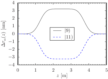
describes the delay (Δ​τ>0)(\Delta\tau>0) or advance (Δ​τ<0)(\Delta\tau<0) of the arrival of the wave packet peak at coordinate zz in the interferometer with respect to that of the free atom.

As a concrete example we consider again the interferometer with the parameters specified in (22) ff. In Figure 5 the roadmap plot is shown for the states α=9\alpha=9 and α=11\alpha=11 in a purely longitudinal magnetic field

𝓑⁡(z)\displaystyle\bm{\mathcal{B}}(z) =ℬ⁡(z)​𝒆3,\displaystyle=\mathcal{B}(z)\bm{e}_{3}\ ,
ℬ⁡(z)\displaystyle\mathcal{B}(z) =10​(e−6​(z−1.25)2−e−6​(z−3.75)2)​μ​T,\displaystyle=10\,\left(e^{-6(z-1.25)^{2}}-e^{-6(z-3.75)^{2}}\right)\,\mu\mathrm{T}\ , (65)

depicted in Figure 4, where zz is taken in meters.

Refer to caption
Figure 4: Example of a magnetic field configuration. The transverse components are chosen as ℬ1=ℬ2=0\mathcal{B}_{1}=\mathcal{B}_{2}=0 and the longitudinal component ℬ⁡(z)\mathcal{B}(z) is given in (65).

We compare the evolution of these states with that of the free 2S, F=1F=1, states (α=9\alpha=9, 1010 and 1111). That is, we set

E0=−L−𝒜32,\displaystyle E_{0}=-L-\frac{\mathcal{A}}{32}\ , (66)

see Table 3 in Appendix D. Here 𝒜\mathcal{A} denotes the ground state hyperfine splitting energy. The potentials for the states α=9\alpha=9 and α=11\alpha=11 are then proportional to the third component of the magnetic field in (65):

V9​(z)\displaystyle V_{9}(z) =g​μB2​ℬ​(z),\displaystyle=\frac{g\mu_{B}}{2}\mathcal{B}(z)\ ,
V11​(z)\displaystyle V_{11}(z) =−g​μB2​ℬ​(z),\displaystyle=-\frac{g\mu_{B}}{2}\mathcal{B}(z)\ , (67)

with the Bohr magneton μB\mu_{B} and the electron’s Landé factor gg, see Table 5 in Appendix D.

Refer to caption
Figure 5: Example of a roadmap plot for the states α=9\alpha=9 and α=11\alpha=11. The corresponding potentials are given in (67).

We see from Figure 5 that in the magnetic field (65) the state α=9\alpha=9 first gets a delay, α=11\alpha=11 an advance compared to the free state. For zz around 3.753.75\,m where the magnetic field is reversed the state α=9\alpha=9 makes up for the delay, the state α=11\alpha=11 for its advance. Finally at z=5z=5\,m they meet again. This gives a nice visualisation of the motion of the wave packet in the interferometer. Clearly, the complete solution contains much more information, as discussed below.

Returning now to the general discussion and putting everything together we find from (38), (48), (3) and (57) the lowest order solution for the wave function as

ψ⁡(𝒙,t,k¯)\displaystyle\psi(\bm{x},t;\bar{k}) =exp⁡[i​γ​(z)]​ψ^​(𝒙,t)\displaystyle=\exp[\mathrm{i}\gamma(z)]\hat{\psi}(\bm{x},t)
=exp⁡[i​ϕ​(z,t)+i​γ​(z)]​𝒜(0)​(𝒙T,ζ,τ)\displaystyle=\exp[\mathrm{i}\phi(z,t)+\mathrm{i}\gamma(z)]{\mathcal{A}}^{(0)}(\bm{x}_{T},\zeta,\tau)
=exp⁡[i​ϕ​(z,t)+i​γ​(z)]​φ​(𝒙T,ζ−τ).\displaystyle=\exp[\mathrm{i}\phi(z,t)+\mathrm{i}\gamma(z)]\varphi(\bm{x}_{T},\zeta-\tau)\ . (68)

For purposes which will become clear in Section 4 we indicate here explicitly also the dependence of ψ\psi on k¯\bar{k}. To write this in a physically transparent form we note that (see (50))

k⁡(z)−k¯\displaystyle k(z)-\bar{k} =k2​(z)−k¯2k⁡(z)+k¯=−2​m​V​(z)k⁡(z)+k¯,\displaystyle=\frac{k^{2}(z)-\bar{k}^{2}}{k(z)+\bar{k}}=-\frac{2mV(z)}{k(z)+\bar{k}}\ ,
∫z0zd​z′​k​(z′)\displaystyle\int^{z}_{z_{0}}\mathrm{d}z^{\prime}k(z^{\prime}) =k¯​(z−z0)+∫z0zd​z′​(k⁡(z′)−k¯)\displaystyle=\bar{k}(z-z_{0})+\int^{z}_{z_{0}}\mathrm{d}z^{\prime}(k(z^{\prime})-\bar{k})
=k¯​(z−z0)−∫z0zd​z′​2​m​V​(z′)k⁡(z′)+k¯.\displaystyle=\bar{k}(z-z_{0})-\int^{z}_{z_{0}}\mathrm{d}z^{\prime}\frac{2mV(z^{\prime})}{k(z^{\prime})+\bar{k}}\ . (69)

We define now

U(z,u;k¯)=exp[−i∫uzdz′2​m​V​(z′)k⁡(z′)+k¯\displaystyle U(z,u;\bar{k})=\exp\left[-\mathrm{i}\int^{z}_{u}\mathrm{d}z^{\prime}\frac{2mV(z^{\prime})}{k(z^{\prime})+\bar{k}}\right.
−12lnk⁡(z)k⁡(u)−12∫uzdz′m​Γ​(z′)k⁡(z′)+iγ(z)−iγ(u)].\displaystyle\left.\qquad-\frac{1}{2}\ln\frac{k(z)}{k(u)}-\frac{1}{2}\int^{z}_{u}\mathrm{d}z^{\prime}\frac{m\Gamma(z^{\prime})}{k(z^{\prime})}+\mathrm{i}\gamma(z)-\mathrm{i}\gamma(u)\right]\ . (70)

It is easy to see that UU corresponds to the evolution of the wave function of an atom at rest with an effective complex mass

ℳ¯eff​(z)\displaystyle\underline{\mathscr{M}}_{\mathrm{eff}}(z) =2​k​(z)k⁡(z)+k¯​V​(z)+i2​k​(z)​∂V⁡(z)∂z\displaystyle=\frac{2k(z)}{k(z)+\bar{k}}V(z)+\frac{\mathrm{i}}{2k(z)}\frac{\partial V(z)}{\partial z}
−i2​Γ​(z)−k⁡(z)m​∂γ⁡(z)∂z.\displaystyle\quad-\frac{\mathrm{i}}{2}\Gamma(z)-\frac{k(z)}{m}\frac{\partial\gamma(z)}{\partial z}\ . (71)

We get

k⁡(z)m​∂U⁡(z,u,k¯)∂z\displaystyle\frac{k(z)}{m}\frac{\partial U(z,u;\bar{k})}{\partial z} =−i​ℳ¯eff​(z)​U​(z,u,k¯),\displaystyle=-\mathrm{i}\underline{\mathscr{M}}_{\mathrm{eff}}(z)U(z,u;\bar{k})\ ,
U⁡(z,u,k¯)|z=u\displaystyle\left.U(z,u;\bar{k})\right|_{z=u} =1.\displaystyle=1\ . (72)

The solution (68) can now be written as

ψ⁡(𝒙,t,k¯)\displaystyle\psi(\bm{x},t;\bar{k}) =exp⁡[−i​k¯22​m​t+i​k¯​(z−z0)]\displaystyle=\exp\left[-\mathrm{i}\frac{\bar{k}^{2}}{2m}t+\mathrm{i}\bar{k}(z-z_{0})\right]
×U⁡(z,u,k¯)|u=𝒵⁡(ζ−τ)​χ​(𝒙τ,ζ−τ)\displaystyle\quad\times\left.U(z,u;\bar{k})\right|_{u=\mathcal{Z}(\zeta-\tau)}\chi{(\bm{x}_{\tau},\zeta-\tau)} (73)

where we define

χ⁡(𝒙T,ζ−τ)=\displaystyle\chi{(\bm{x}_{T},\zeta-\tau)}=
exp[−i∫z0udz′2​m​V​(z′)k⁡(z′)+k¯+iγ(u)]|u=𝒵⁡(ζ−τ)\displaystyle\qquad\left.\exp\left[-\mathrm{i}\int^{u}_{z_{0}}\mathrm{d}z^{\prime}\frac{2mV(z^{\prime})}{k(z^{\prime})+\bar{k}}+\mathrm{i}\gamma(u)\right]\right|_{u=\mathcal{Z}(\zeta-\tau)}
×φ⁡(𝒙T,ζ−τ).\displaystyle\qquad\quad\times\varphi(\bm{x}_{T},\zeta-\tau)\ . (74)

For τ=0\tau=0 we have u=𝒵⁡(ζ)=zu=\mathcal{Z}(\zeta)=z and U⁡(z,u,k¯)=1U(z,u;\bar{k})=1. Thus,

ψ⁡(𝒙,t,k¯)|t=0=exp⁡[i​k¯​(z−z0)]​χ​(𝒙T,ζ)|ζ=ℨ⁡(z)\displaystyle\left.\psi(\bm{x},t;\bar{k})\right|_{t=0}=\exp[\mathrm{i}\bar{k}(z-z_{0})]\left.\chi(\bm{x}_{T},\zeta)\right|_{\zeta={\mathfrak{Z}}(z)} (75)

contains a plane wave factor and χ⁡(𝒙T,ζ)\chi(\bm{x}_{T},\zeta), the envelope amplitude at t=0t=0. The interpretation of the result (73) is then as follows. The wave function ψ⁡(𝒙,t,k¯)\psi(\bm{x},t;\bar{k}) contains a plane wave factor and a factor U⁡(z,u)U(z,u) corresponding to the complex phase picked up by the atom travelling from u=𝒵⁡(ζ−τ)u=\mathcal{Z}(\zeta-\tau) to z=𝒵⁡(ζ)z=\mathcal{Z}(\zeta). This is multiplied with the shifted original envelope amplitude χ⁡(𝒙T,ζ−τ)\chi(\bm{x}_{T},\zeta-\tau). The factor U⁡(z,u,k¯)U(z,u;\bar{k}) corresponds to the evolution of the atom at rest with the complex mass ℳ¯eff​(z)\underline{\mathscr{M}}_{\mathrm{eff}}(z) (71). From (70) we see that UU contains, in general, complex dynamical and geometric phases. In this way we make the connection to [11, 12] where such phases were studied for atoms at rest.

A typical ansatz for the initial envelope amplitude χ\chi in (73)–(75) is a Gaussian

χ⁡(𝒙T,ζ)\displaystyle\chi(\bm{x}_{T},\zeta) =𝒩(2π)−3/4σT−1σL−1/2\displaystyle={\cal N}(2\pi)^{-3/4}\sigma^{-1}_{T}\sigma^{-1/2}_{L}
×exp⁡(−14​σT2​𝒙T2−14​σL2​ζ2),\displaystyle\quad\times\exp\left(-\frac{1}{4\sigma^{2}_{T}}\bm{x}^{2}_{T}-\frac{1}{4\sigma^{2}_{L}}\zeta^{2}\right)\ ,
σT,σL\displaystyle\sigma_{T},\sigma_{L} >0.\displaystyle>0\ . (76)

Here 𝒩>0{\cal N}>0 is a normalisation factor, σT\sigma_{T} the transverse and σL\sigma_{L} the longitudinal width, respectively. Supposing that at t=0t=0 we have exactly one atom in this wave we get 𝒩{\cal N} from

∫d3​x​|ψ⁡(𝒙,t,k¯)|2|t=0=∫d2​xT​∫d​z​|χ⁡(𝒙T,ℨ⁡(z))|2=1.\displaystyle\int\mathrm{d}^{3}x\left.|\psi(\bm{x},t;\bar{k})|^{2}\right|_{t=0}=\int\mathrm{d}^{2}x_{T}\int\mathrm{d}z\,|\chi(\bm{x}_{T},{\mathfrak{Z}}(z))|^{2}=1\ . (77)

In Appendix B we study the first correction term in the series (55) for the function (76). We find that for the interferometer parameters specified in (22) ff. the zero order solution (73) is valid with a 1%1\% accuracy in the region of interest provided

σL\displaystyle\sigma_{L} >100​μ​m,\displaystyle>100\,\mathrm{\mu m}\ ,
σT\displaystyle\sigma_{T} >100​μ​m,\displaystyle>100\,\mathrm{\mu m}\ , (78)

see (B.64)–(B.66). Under typical experimental conditions [1] the actual longitudinal widths of the wave packets used are of order 0.40.4\,nm, that is, much smaller than those in (78), while σT\sigma_{T} can indeed be of order 100​μ​m100\,\mathrm{\mu m}. Such wave packets are described as superpositions of the solutions (73) which serve as wavelets in the analysis, see Section 4.

4 Interference effects

In this section we shall study, as a concrete example, interference effects of two 2S states travelling through the interferometer specified in (22) ff. Of course, the formulas given below are easily adapted to other experimental setups and more than two states.

Let us consider the case that we have at time t=0t=0 two narrow wave packets around z≈z0z\approx z_{0} in the interferometer of (22) ff. These wave packets are supposed to form a coherent superposition of two components |α(z0))|\alpha(z_{0})) and |β(z0))|\beta(z_{0})) of the 2S states where

α,β∈I⊂{9,10,11,12}.\displaystyle\alpha,\beta\in I\subset\{9,10,11,12\}\ . (79)

Here II is defined as an index set with two elements. The two waves travel through the interferometer and are supposed to be analysed at z=zaz=z_{a} as discussed below. For the initial state we make the following ansatz

|Ψ(𝒙,t)⟩|t=0=Ψ(𝒙,0)∑α∈Icα|α(z0))\displaystyle\left.|\Psi(\bm{x},t)\rangle\right|_{t=0}=\Psi(\bm{x},0)\sum_{\alpha\in I}c_{\alpha}|\alpha(z_{0})) (80)

with

∑α∈I|cα|2=1\displaystyle\sum_{\alpha\in I}|c_{\alpha}|^{2}=1 (81)

and

Ψ⁡(𝒙,0)=∫d​k¯2​π​f​(k¯)​exp⁡[i​k¯​(z−z0)]​χ​(𝒙T,z−z0).\displaystyle\Psi(\bm{x},0)=\int\frac{\mathrm{d}\bar{k}}{2\pi}f(\bar{k})\exp[\mathrm{i}\bar{k}(z-z_{0})]\chi(\bm{x}_{T},z-z_{0})\ . (82)

Here and in the following all integrals run from −∞-\infty to +∞+\infty if not indicated otherwise. This initial wave function is supposed to be non zero only in the field free region around z0z_{0}. Taking into account (78) we shall now suppose that the parameter δ​l\delta l specifying the field free region in (13) has the value

δ​l=10​mm.\displaystyle\delta l=10\,\mathrm{mm}\ . (83)

Note that for zero external fields the initial states |α(z0))|\alpha(z_{0})) with α∈I\alpha\in I are orthonormal in the ordinary sense since these states have different values (F,F3)(F,F_{3}) which are “good” quantum numbers for 𝓔=𝓑=𝟎\bm{\mathcal{E}}=\bm{\mathcal{B}}=\bm{0}, see Table 2 of Appendix A. In (82) χ⁡(𝒙T,z−z0)\chi(\bm{x}_{T},z-z_{0}) is an envelope amplitude with widths in transverse and longitudinal directions

δ​l=10​mm≫σT,σL≳100​μ​m.\displaystyle\delta l=10\,\mathrm{mm}\gg\sigma_{T},\sigma_{L}\gtrsim 100\,\mathrm{\mu m}\ . (84)

We suppose the normalisation condition

∫d2​xT​∫d​z​|χ⁡(𝒙T,z−z0)|2=1\displaystyle\int\mathrm{d}^{2}x_{T}\int\mathrm{d}z\,|\chi(\bm{x}_{T},z-z_{0})|^{2}=1 (85)

to hold, see (77) with ℨ⁡(z)=z−z0\mathfrak{Z}(z)=z-z_{0}. The Fourier transform of χ\chi is denoted by

χ~​(𝒒T,qL)=∫d2​xT′​∫d​z′​exp⁡(−i​𝒒TCLOSE\displaystyle\tilde{\chi}(\bm{q}_{T},q_{L})=\int\mathrm{d}^{2}x^{\prime}_{T}\int\mathrm{d}z^{\prime}\exp(-\mathrm{i}\bm{q}_{T} OPEN𝒙T′−i​qL​z′)\displaystyle\bm{x}^{\prime}_{T}-\mathrm{i}q_{L}z^{\prime})
×χ⁡(𝒙T′,z′).\displaystyle\times\chi(\bm{x}^{\prime}_{T},z^{\prime})\ . (86)

We superpose functions χ\chi in (82) using a function f⁡(k¯)f(\bar{k}) which is supposed to have a sharp peak at k¯=k¯m\bar{k}=\bar{k}_{m} (mm for maximum) and a width Δ​k¯=σk−1\Delta\bar{k}=\sigma^{-1}_{k} with

0<σk≪σL,k¯m≫σk−1.\displaystyle 0<\sigma_{k}\ll\sigma_{L},\;\bar{k}_{m}\gg\sigma^{-1}_{k}\ . (87)

We require the state in (80) to be normalised which implies

∫d3​x​|Ψ⁡(𝒙,0)|2\displaystyle\int\mathrm{d}^{3}x|\Psi(\bm{x},0)|^{2} =∫d​k¯′​d​k¯(2​π)2​f∗​(k¯′)​f​(k¯)\displaystyle=\int\frac{\mathrm{d}\bar{k}^{\prime}\mathrm{d}\bar{k}}{(2\pi)^{2}}\,f^{*}(\bar{k}^{\prime})f(\bar{k})
×∫d2​xT′​∫d​z′​exp⁡[i⁡(k¯−k¯′)​z′]\displaystyle\qquad\times\int\mathrm{d}^{2}x^{\prime}_{T}\int\mathrm{d}z^{\prime}\exp[\mathrm{i}(\bar{k}-\bar{k}^{\prime})z^{\prime}]
×|χ⁡(𝒙T′,z′)|2\displaystyle\qquad\times|\chi(\bm{x}^{\prime}_{T},z^{\prime})|^{2}
=1.\displaystyle=1\ . (88)

We define the Fourier transform of Ψ⁡(𝒙,0)\Psi(\bm{x},0) in (82) as

Ψ~​(𝒒T,qL)\displaystyle\tilde{\Psi}(\bm{q}_{T},q_{L})
=∫d2​xT​∫d​z​exp⁡(−i​𝒒T​𝒙T−i​qL​(z−z0))​Ψ​(𝒙,0)\displaystyle\quad=\int\mathrm{d}^{2}x_{T}\int\mathrm{d}z\exp(-\mathrm{i}\bm{q}_{T}\bm{x}_{T}-\mathrm{i}q_{L}(z-z_{0}))\Psi(\bm{x},0)
=∫d​k¯2​π​f​(k¯)​χ~​(𝒒T,qL−k¯).\displaystyle\quad=\int\frac{\mathrm{d}\bar{k}}{2\pi}f(\bar{k})\tilde{\chi}(\bm{q}_{T},q_{L}-\bar{k})\ . (89)

Equations (79) to (89) define the general type of wave functions for which we shall calculate interference effects below. For later use, we define Gaussian functions as concrete examples for such wave functions:

χ⁡(𝒙T,z−z0)\displaystyle\chi(\bm{x}_{T},z-z_{0}) =(2π)−3/4σT−1σL−1/2\displaystyle=(2\pi)^{-3/4}\sigma^{-1}_{T}\sigma^{-1/2}_{L}
×exp⁡[−14​σT2​𝒙T2−14​σL2​(z−z0)2],\displaystyle\quad\times\exp\left[-\frac{1}{4\sigma^{2}_{T}}\bm{x}^{2}_{T}-\frac{1}{4\sigma^{2}_{L}}(z-z_{0})^{2}\right], (90)
f⁡(k¯)\displaystyle f(\bar{k}) =(4​π​σk)1/2​(σk2+σL2)1/4\displaystyle=(4\pi\sigma_{k})^{1/2}(\sigma^{2}_{k}+\sigma^{2}_{L})^{1/4}
×exp⁡[−σk2​(k¯−k¯m)2]\displaystyle\quad\times\exp\left[-\sigma^{2}_{k}(\bar{k}-\bar{k}_{m})^{2}\right] (91)

with 10​mm≫σT10\,\mathrm{mm}\gg\sigma_{T}, σL≥100​μ​m\sigma_{L}\geq 100\,\mathrm{\mu m} and σk≪σL\sigma_{k}\ll\sigma_{L}. We get then

χ~​(𝒒T,qL)\displaystyle\tilde{\chi}(\bm{q}_{T},q_{L}) =(2​π)3/4​2​σT​2​σL\displaystyle=(2\pi)^{3/4}2\sigma_{T}\sqrt{2\sigma_{L}}
×exp⁡(−σT2​𝒒T2−σL2​qL2),\displaystyle\quad\times\exp(-\sigma^{2}_{T}\bm{q}^{2}_{T}-\sigma^{2}_{L}q^{2}_{L})\ , (92)
Ψ~​(𝒒T,qL)\displaystyle\tilde{\Psi}(\bm{q}_{T},q_{L}) =(2​π)3/4​2​σT​2​σk′\displaystyle=(2\pi)^{3/4}2\sigma_{T}\sqrt{2\sigma^{\prime}_{k}}
×exp⁡[−σT2​𝒒T2−σk′2​(qL−k¯m)2]\displaystyle\quad\times\exp[-\sigma^{2}_{T}\bm{q}^{2}_{T}-\sigma^{\prime 2}_{k}(q_{L}-\bar{k}_{m})^{2}] (93)

where

σk′=σk​σLσL2+σk2.\displaystyle\sigma^{\prime}_{k}=\frac{\sigma_{k}\sigma_{L}}{\sqrt{\sigma^{2}_{L}+\sigma^{2}_{k}}}\ . (94)

Note that for σk≪σL\sigma_{k}\ll\sigma_{L} we have σk′≈σk\sigma^{\prime}_{k}\approx\sigma_{k}.

The evolution of the general state (80) with time is obtained from the results of Section 3. Here, of course, we have to reinstate the index α\alpha on all quantities. Thus we have potentials 𝒱α\mathcal{V}_{\alpha}, variables ζα\zeta_{\alpha}, final solutions (73) ψα​(𝒙,t,k¯)\psi_{\alpha}(\bm{x},t;\bar{k}), etc. We get in this way from the initial state (80) the solution

|Ψ(𝒙,t)⟩=∫d​k¯2​πf(k¯)∑α∈Icαψα(𝒙,t;k¯)|α(z))\displaystyle|\Psi(\bm{x},t)\rangle=\int\frac{\mathrm{d}\bar{k}}{2\pi}f(\bar{k})\sum_{\alpha\in I}c_{\alpha}\psi_{\alpha}(\bm{x},t;\bar{k})|\alpha(z)) (95)

where

ψα​(𝒙,t,k¯)\displaystyle\psi_{\alpha}(\bm{x},t;\bar{k}) =exp⁡[−i​k¯22​m​t+i​k¯​(z−z0)]\displaystyle=\exp\left[-\mathrm{i}\frac{\bar{k}^{2}}{2m}t+\mathrm{i}\bar{k}(z-z_{0})\right]
×Uα​(z,u,k¯)|u=𝒵α​(ℨα​(z)−(k¯/m)​t)\displaystyle\quad\times\left.U_{\alpha}(z,u;\bar{k})\right|_{u=\mathcal{Z}_{\alpha}({\mathfrak{Z}}_{\alpha}(z)-(\bar{k}/m)t)}
×χ⁡(𝒙T,ℨα​(z)−(k¯/m)​t).\displaystyle\quad\times\chi(\bm{x}_{T},{\mathfrak{Z}}_{\alpha}(z)-(\bar{k}/m)t)\ . (96)

Now we come to the analysis of the state (95) at z=zaz=z_{a} where again we have a field free region for zz several σL\sigma_{L} around zaz_{a}, see (13) and (84). We have, therefore,

|α(z))=|α(za))=|α(z0))\displaystyle|\alpha(z))=|\alpha(z_{a}))=|\alpha(z_{0}))\ (97)

for |z−za|<δ​l=10​mm|z-z_{a}|<\delta l=10\,\mathrm{mm}. We suppose that the state (95) is projected onto

|p)=∑α∈Ipα|α(z0))\displaystyle|p)=\sum_{\alpha\in I}p_{\alpha}|\alpha(z_{0})) (98)

where

∑α∈I|pα|2=1.\displaystyle\sum_{\alpha\in I}|p_{\alpha}|^{2}=1\ . (99)

This gives

|Ψp(𝒙,t)⟩=|p)(p~|Ψ(𝒙,t)⟩=Ψp(𝒙,t)|p)\displaystyle|\Psi_{p}(\bm{x},t)\rangle=|p)(\widetilde{p}|\,\Psi(\bm{x},t)\rangle=\Psi_{p}(\bm{x},t)|p) (100)

with

(p~|=∑α∈I(α⁡(z0)~|pα∗CLOSECLOSE,\displaystyle(\widetilde{p}|=\sum_{\alpha\in I}(\widetilde{\alpha(z_{0})}|p^{*}_{\alpha}\ , (101)
Ψp​(𝒙,t)\displaystyle\Psi_{p}(\bm{x},t) =(p~|Ψ(𝒙,t)⟩\displaystyle=(\widetilde{p}|\Psi(\bm{x},t)\rangle
=∫d​k¯2​π​f​(k¯)​∑α∈Ipα∗​cα​ψα​(𝒙,t,k¯).\displaystyle=\int\frac{\mathrm{d}\bar{k}}{2\pi}f(\bar{k})\sum_{\alpha\in I}p^{*}_{\alpha}c_{\alpha}\psi_{\alpha}(\bm{x},t;\bar{k})\ . (102)

We suppose that the total integrated flux ℱp{\cal F}_{p} in the above projection is measured at z=zaz=z_{a}. This is given by

ℱp=∫d​t​∫d2​xT​jz​(𝒙T,za,t)\displaystyle{\cal F}_{p}=\int\mathrm{d}t\int\mathrm{d}^{2}x_{T}\,j_{z}(\bm{x}_{T},z_{a},t) (103)

where the zz-component of the probability current is

jz​(𝒙T,z,t)=12​m​i​Ψp∗​(𝒙,t)​∂∂z​Ψp​(𝒙,t)+c.c..\displaystyle j_{z}(\bm{x}_{T},z,t)=\frac{1}{2m\mathrm{i}}\Psi^{*}_{p}(\bm{x},t)\frac{\partial}{\partial z}\Psi_{p}(\bm{x},t)+\mathrm{c.c.}\ . (104)

In evaluating jzj_{z} and ℱp{\cal F}_{p} we take into account (87). We get then, as explained in detail in Appendix C, the following results

jz​(𝒙T,za,t)=k¯mm​Ψp∗​(𝒙T,za,t)​Ψp​(𝒙T,za,t),\displaystyle j_{z}(\bm{x}_{T},z_{a},t)=\frac{\bar{k}_{m}}{m}\Psi^{*}_{p}(\bm{x}_{T},z_{a},t)\Psi_{p}(\bm{x}_{T},z_{a},t)\ , (105)
ℱp=∫d​k¯s2​π\displaystyle{\cal F}_{p}=\int\frac{\mathrm{d}\bar{k}_{s}}{2\pi} ∑α,β∈I{pβpα∗cβ∗cαg(k¯s,Δτβ,Δτα)\displaystyle\sum_{\alpha,\beta\in I}\Big\{p_{\beta}p^{*}_{\alpha}c^{*}_{\beta}c_{\alpha}g(\bar{k}_{s},\Delta\tau_{\beta},\Delta\tau_{\alpha})
×exp⁡[−i⁡(k¯s−k¯m)​(Δ​τβ−Δ​τα)]\displaystyle\times\exp[-\mathrm{i}(\bar{k}_{s}-\bar{k}_{m})(\Delta\tau_{\beta}-\Delta\tau_{\alpha})]
×Uβ∗(za,z0;k¯m)Uα(za,z0;k¯m)}.\displaystyle\times U^{*}_{\beta}(z_{a},z_{0};\bar{k}_{m})U_{\alpha}(z_{a},z_{0};\bar{k}_{m})\Big\}\ . (106)

In (105), (106) and in the following only the leading terms for large k¯m\bar{k}_{m} are kept. In analogy to (64) we define, with k¯=k¯m\bar{k}=\bar{k}_{m}, the shift of the reduced arrival times at z=zaz=z_{a} to be

Δ​τα=ℨα​(za)−(za−z0)=mk¯m2​∫z0zad​z′​Vα​(z′)\displaystyle\Delta\tau_{\alpha}={\mathfrak{Z}}_{\alpha}(z_{a})-(z_{a}-z_{0})=\frac{m}{\bar{k}^{2}_{m}}\int^{z_{a}}_{z_{0}}\mathrm{d}z^{\prime}\,V_{\alpha}(z^{\prime}) (107)

with 𝒪⁡(k¯m−3)\mathcal{O}(\bar{k}_{m}^{-3}) terms neglected, see (C.5) and (C.6). Furthermore, we introduce the function

g⁡(k¯s,Δ​τβ,Δ​τα)=∫d​k¯d2​π​f∗​(k¯s−12​k¯d)​f​(k¯s+12​k¯d)\displaystyle g(\bar{k}_{s},\Delta\tau_{\beta},\Delta\tau_{\alpha})=\int\frac{\mathrm{d}\bar{k}_{d}}{2\pi}f^{*}(\bar{k}_{s}-\frac{1}{2}\bar{k}_{d})f(\bar{k}_{s}+\frac{1}{2}\bar{k}_{d})
×∫d​z′​∫d2​xT​exp⁡[i​k¯d​(z′+12​Δ​τβ+12​Δ​τα)]\displaystyle\times\int\mathrm{d}z^{\prime}\int\mathrm{d}^{2}x_{T}\exp\left[\mathrm{i}\bar{k}_{d}\left(z^{\prime}+\frac{1}{2}\Delta\tau_{\beta}+\frac{1}{2}\Delta\tau_{\alpha}\right)\right]
×χ∗​(𝒙T,z′+Δ​τβ)​χ​(𝒙T,z′+Δ​τα).\displaystyle\qquad\qquad\times\chi^{*}(\bm{x}_{T},z^{\prime}+\Delta\tau_{\beta})\chi(\bm{x}_{T},z^{\prime}+\Delta\tau_{\alpha})\ . (108)

From (70) we get with k¯=k¯m\bar{k}=\bar{k}_{m} and k⁡(z0)=k⁡(za)=k¯mk(z_{0})=k(z_{a})=\bar{k}_{m},

Uα​(za,z0,k¯m)=exp⁡[−i​ϕdyn,α+i​ϕgeom,α]\displaystyle U_{\alpha}(z_{a},z_{0};\bar{k}_{m})=\exp[-\mathrm{i}\phi_{\mathrm{dyn},\alpha}+\mathrm{i}\phi_{\mathrm{geom},\alpha}] (109)

where the complex dynamical and geometrical phases are

ϕdyn,α\displaystyle\phi_{\mathrm{dyn},\alpha} =mk¯m​∫z0zad​z′​[Vα​(z′)−i2​Γα​(z′)],\displaystyle=\frac{m}{\bar{k}_{m}}\int^{z_{a}}_{z_{0}}\mathrm{d}z^{\prime}[V_{\alpha}(z^{\prime})-\frac{\mathrm{i}}{2}\Gamma_{\alpha}(z^{\prime})]\ , (110)
ϕgeom,α\displaystyle\phi_{\mathrm{geom},\alpha} =γα​α​(za)−γα​α​(z0).\displaystyle=\gamma_{\alpha\alpha}(z_{a})-\gamma_{\alpha\alpha}(z_{0})\ . (111)

In (110) terms of 𝒪⁡(k¯m−2)\mathcal{O}(\bar{k}_{m}^{-2}) are neglected. From (107) and (110) we find

Re​ϕdyn,α=k¯m​Δ​τα.\displaystyle\mathrm{Re}\,\phi_{\mathrm{dyn},\alpha}=\bar{k}_{m}\Delta\tau_{\alpha}\ . (112)

In (106)–(112) we have given our general result for the integrated flux ℱp{\cal F}_{p} of the atom in the state |p)|p) where we supposed large k¯m\bar{k}_{m}, see Appendix C. That is, (106)–(112) are valid for all wave packets of the type described in (80)–(89). We insert now the Gaussian distributions for χ\chi and ff, see (90)–(94). After a simple calculation presented in Appendix C we obtain for this case for ℱp\mathcal{F}_{p}, an easily accessible observable for lABSE experiments, the result:

ℱp=∑α,β∈I\displaystyle{\cal F}_{p}=\sum_{\alpha,\beta\in I} pβpα∗cβ∗cαexp[−(Δτβ−Δτα)2/(8σk′2)]\displaystyle p_{\beta}p^{*}_{\alpha}c^{*}_{\beta}c_{\alpha}\exp[-(\Delta\tau_{\beta}-\Delta\tau_{\alpha})^{2}/(8\sigma^{\prime 2}_{k})]
×Uβ∗​(za,z0,k¯m)​Uα​(za,z0,k¯m).\displaystyle\quad\times U^{*}_{\beta}(z_{a},z_{0};\bar{k}_{m})U_{\alpha}(z_{a},z_{0};\bar{k}_{m})\ . (113)

As a concrete application we discuss our result (113) for the following field configuration. We choose the electric field as 𝓔⁡(z)=𝟎\bm{\mathcal{E}}(z)=\bm{0} and the magnetic field similar to (65)

𝓑⁡(z)\displaystyle\bm{\mathcal{B}}(z) =ℬ⁡(z)​𝒆3,\displaystyle=\mathcal{B}(z)\bm{e}_{3}\ ,
ℬ⁡(z)\displaystyle\mathcal{B}(z) =10​(e−6​(z−1.25)2−s⋅e−6​(z−3.75)2)​μ​T,\displaystyle=10\,\big(e^{-6(z-1.25)^{2}}-s\cdot e^{-6(z-3.75)^{2}}\big)\,\mu\mathrm{T}\ , (114)

where a parameter ss is inserted in order to detune the second half of the magnetic field configuration around the symmetric arrangement, see Figure 6. The reason for the introduction of ss will be discussed below. Note that such magnetic fields can be produced by suitably shaped coils. The so-called spin echo coil produces the scalable part of 𝓑⁡(z)\bm{\mathcal{B}}(z) via controlling the electric current through the coil.

Refer to caption
Figure 6: The magnetic field as used for the calculations in this section is shown for several values of the parameter ss from (114).

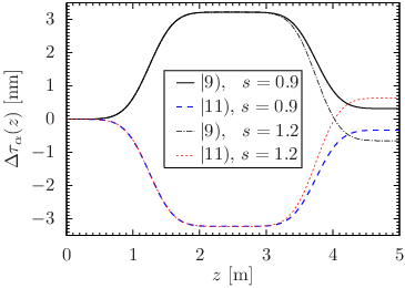
Figure 7 illustrates the global behaviour of the two states α=9\alpha=9 and α=11\alpha=11 for different values of ss. Setting s=1s=1 leads to the roadmap plot shown in Figure 5. Considering s=0.9s=0.9, the state α=9\alpha=9 accumulates a delay compared to a free wave, while the state α=11\alpha=11 picks up an advance. The opposite is true for s=1.2s=1.2.

Refer to caption
Figure 7: Two examples of the roadmap plots for the states α=9\alpha=9 and α=11\alpha=11 based on the magnetic field (114) and 𝓔⁡(z)=𝟎\bm{\mathcal{E}}(z)=\bm{0} with fixed parameters s=0.9s=0.9 and s=1.2s=1.2 respectively.

Eventually, the evaluation of the total integrated flux ℱp\mathcal{F}_{p} is shown in Figure 8. In our calculation we choose for the initial wave packet Gaussian momentum distributions for the functions in (90)–(93) with

k¯m\displaystyle\bar{k}_{m} =5.6×10¹⁰​m−1,\displaystyle=5.6\times 10^{10}\,\mathrm{m}^{-1}\ , (115)
σL\displaystyle\sigma_{L} =σT=100​μ​m,\displaystyle=\sigma_{T}=100\,\mu\mathrm{m}\ , (116)
σk′\displaystyle\sigma^{\prime}_{k} =0.4​nm.\displaystyle=0.4\,\mathrm{nm}\ . (117)

Furthermore, we choose the coefficients cαc_{\alpha} of the initial state the same as those of the analysing state, namely

c9=c11=p9=p11=12.\displaystyle c_{9}=c_{11}=p_{9}=p_{11}=\frac{1}{\sqrt{2}}\ . (118)

The initial state is then according to (80) and (89)

|Ψ⁡(𝒙,t)⟩|t=0\displaystyle\left.|\Psi(\bm{x},t)\rangle\right|_{t=0} =Ψ(𝒙,0)12(|9)+|11))|𝓔=𝓑=𝟎,\displaystyle=\Psi(\bm{x},0)\frac{1}{\sqrt{2}}\left.\big(|9)+|11)\big)\right|_{\bm{\mathcal{E}}=\bm{\mathcal{B}}=\bm{0}}\ , (119)
Ψ⁡(𝒙,0)\displaystyle\Psi(\bm{x},0) =∫d2​qT​d​qL(2​π)3​exp⁡[i​𝒒T​𝒙T+i​qL​(z−z0)]​Ψ~​(𝒒T,qL)\displaystyle=\int\frac{\mathrm{d}^{2}q_{T}\mathrm{d}q_{L}}{(2\pi)^{3}}\exp[\mathrm{i}\bm{q}_{T}\bm{x}_{T}+\mathrm{i}q_{L}(z-z_{0})]\,\tilde{\Psi}(\bm{q}_{T},q_{L})
=(2π)−3/4σT−1(σk′)−1/2exp[ik¯m(z−z0)]\displaystyle=(2\pi)^{-3/4}\sigma^{-1}_{T}(\sigma^{\prime}_{k})^{-1/2}\,\exp[\mathrm{i}\bar{k}_{m}(z-z_{0})]
×exp⁡[−14​σT2​𝒙T2−14​σk′2​(z−z0)2].\displaystyle\times\exp\left[-\frac{1}{4\sigma^{2}_{T}}\bm{x}^{2}_{T}-\frac{1}{4\sigma^{\prime 2}_{k}}(z-z_{0})^{2}\right]\ . (120)

Thus, with the choice (118) we superpose the states α=9\alpha=9 and α=11\alpha=11 at z0=0z_{0}=0 and project the evolved state at za=5z_{a}=5\,m onto the same superposition.

Refer to caption
Figure 8: The total integrated flux for the magnetic field in (114) with the parameter ss varied over the interval [0.7,1.3][0.7,1.3]. Every value of ss leads to a fixed flux of analysing states.

The signal to be observed experimentally is the integrated flux as function of the parameter ss at a fixed point on the z-axis, in our case at the final point za=5z_{a}=5\,m of the interferometer, see Figure 8. A variation of ss alters the terms (Δ​τβ−Δ​τα)(\Delta\tau_{\beta}-\Delta\tau_{\alpha}) in (113) as well as the dynamical phases ϕdyn\phi_{\mathrm{dyn}} in (110). Thus, with the simple field configuration of Figure 6 it should be possible to create an interference signal simply by tuning the current of the spin echo coil and counting outgoing atoms. This signal could serve as a reference for more complicated field configurations.

Let us now consider a configuration with magnetic and electric fields as a second example. We define the functions

ℬ⁡(z)\displaystyle\mathcal{B}(z) =10​(e−10​(z−0.75)2+e−10​(z−1.75)2CLOSE\displaystyle=10\,\big(e^{-10(z-0.75)^{2}}+e^{-10(z-1.75)^{2}}
OPEN−e−10​(z−3.25)2−e−10​(z−4.25)2)\displaystyle\qquad\qquad-e^{-10(z-3.25)^{2}}-e^{-10(z-4.25)^{2}}\big) (121)

and

ℰ⁡(z)=e−300​(z−0.9)2+e−300​(z−1.6)2\displaystyle\mathcal{E}(z)=e^{-300(z-0.9)^{2}}+e^{-300(z-1.6)^{2}} (122)

where zz is given in meters. Now we choose the magnetic field 𝓑⁡(𝒛)\bm{\mathcal{B}(z)}, given in μ​T\mu\mathrm{T}, and the electric field 𝓔⁡(𝒛)\bm{\mathcal{E}(z)}, given in V/cm\mathrm{V/cm}, as follows

ℬ1=ℬ2=0,ℬ3={ℬ⁡(z),z∈[0,0.75]∪[1.75,2.5],ℬ⁡(0.75),z∈[0.75,1.75],s⋅ℬ⁡(z),z∈[2.5,3.25]∪[4.25,5],s⋅ℬ⁡(3.25),z∈[3.25,4.25],\displaystyle\begin{split}\mathcal{B}_{1}&=\mathcal{B}_{2}=0\ ,\\ \mathcal{B}_{3}&=\left\{\begin{array}[]{rl}\mathcal{B}(z)&,\;z\in[0,0.75]\cup[1.75,2.5]\,,\\ \mathcal{B}(0.75)&,\;z\in[0.75,1.75]\,,\\ s\cdot\mathcal{B}(z)&,\;z\in[2.5,3.25]\cup[4.25,5]\,,\\ s\cdot\mathcal{B}(3.25)&,\;z\in[3.25,4.25]\,,\end{array}\right.\ \end{split} (123)

and

ℰ1={ℰ⁡(z),z∈[0,0.9]∪[1.6,5],ℰ⁡(0.9),z∈[0.9,1.6],ℰ2=ℰ3=0,\displaystyle\begin{split}\mathcal{E}_{1}&=\left\{\begin{array}[]{rl}\mathcal{E}(z)&,\;z\in[0,0.9]\cup[1.6,5]\,,\\ \mathcal{E}(0.9)&,\;z\in[0.9,1.6]\,,\end{array}\right.\\ \mathcal{E}_{2}&=\mathcal{E}_{3}=0\ ,\end{split} (124)

respectively. In Figure 9 we show ℬ3​(z)\mathcal{B}_{3}(z) and ℰ1​(z)\mathcal{E}_{1}(z). The electric field is ramped to a constant value and back again only within a region of constant magnetic field. This procedure implies vanishing geometric phases.

Refer to caption
Figure 9: The magnetic field component ℬ3​(z)\mathcal{B}_{3}(z) (123), solid line, and the electric field component ℰ1​(z)\mathcal{E}_{1}(z) (124), given as the dashed line.

For the calculation of the spin echo signal with the external fields (123) and (124), we again employ the initial specifications (115)–(120). The results for both the pure magnetic field and the combined magnetic and electric fields are shown in Figure 10. In the presence of the electric field 𝓔\bm{\mathcal{E}}, we find a decreased total integrated flux ℱp𝓔≠𝟎​(s)\mathcal{F}^{\bm{\mathcal{E}}\not=\bm{0}}_{p}(s) due to the enhanced decay rate, compared to the case of ℱp𝓔=𝟎​(s)\mathcal{F}^{\bm{\mathcal{E}}=\bm{0}}_{p}(s).

Refer to caption
Figure 10: The spin echo signal corresponding to the case where only the magnetic field (123) is present is given by the (red) dashed line. The spin echo signal corresponding to the presence of the magnetic field (123) and the electric field (124) is given by the solid line.

In order to interpret Figure 10, we now give an estimate of the quantities which lead to the altered spin echo signal when the electric field (124) is switched on. For 𝓔≠0\bm{\mathcal{E}}\not=0 the quadratic Stark effect leads to a shift of the complex energies EαE_{\alpha}. The shift of the real parts VαV_{\alpha} of EαE_{\alpha} turns out to be negligible. Therefore, the reduced arrival times do not change substantially compared to the case of 𝓔=0\bm{\mathcal{E}}=0. The change of the oscillation frequency of ℱp𝓔≠𝟎​(s)\mathcal{F}^{\bm{\mathcal{E}}\not=\bm{0}}_{p}(s), induced by VαV_{\alpha}, is also not significant if we compare to ℱp𝓔=𝟎​(s)\mathcal{F}^{\bm{\mathcal{E}}=\bm{0}}_{p}(s), see Figure 10. However, the altered imaginary parts −12​Γα-\frac{1}{2}\Gamma_{\alpha} have a large impact on the total integrated flux via the dynamical phases. For the case of the non-zero electric field (124), we get for the states α=9\alpha=9, 1010 and 1111 the relation

Γα𝓔≠𝟎​(z)\displaystyle\Gamma^{\bm{\mathcal{E}}\not=\bm{0}}_{\alpha}(z) ≈300​Γα(𝓔=𝟎)​(z)\displaystyle\approx 300\,\Gamma^{(\bm{\mathcal{E}}=\bm{0})}_{\alpha}(z)
≈300​ΓS≈2470​s−1\displaystyle\approx 300\,\Gamma_{S}\approx 2470\,\mathrm{s}^{-1} (125)

for the parameter range 0.85≲z≲1.650.85\lesssim z\lesssim 1.65, where ΓS\Gamma_{S} is given in (26). Taking into account that in this case the geometric phases are zero and considering (113) together with (109) and (110), we find for s=1s=1:

ℱp(𝓔≠𝟎)​(s=1)\displaystyle\mathcal{F}^{(\bm{\mathcal{E}}\not=\bm{0})}_{p}(s=1) ≈exp(−mkm 300∫z=0.85​mz=1.65​mdz′ΓS)\displaystyle\approx\exp\big(-\frac{m}{k_{m}}\,300\int^{z=1.65\,\mathrm{m}}_{z=0.85\,\mathrm{m}}\mathrm{d}z^{\prime}\Gamma_{S}\big)
×ℱp(𝓔=𝟎)​(s=1).\displaystyle\qquad\times\mathcal{F}^{(\bm{\mathcal{E}}=\bm{0})}_{p}(s=1)\ . (126)

Inserting

mkm=^(3500​m/s)−1,\displaystyle\frac{m}{k_{m}}\mathrel{\widehat{=}}(3500\,\mathrm{m}/\mathrm{s})^{-1}\ , (127)

we get

ℱp(𝓔≠𝟎)​(s=1)≈0.569​ℱp(𝓔=𝟎)​(s=1)≈0.562.\displaystyle\mathcal{F}^{(\bm{\mathcal{E}}\not=\bm{0})}_{p}(s=1)\approx 0.569\,\mathcal{F}^{(\bm{\mathcal{E}}=\bm{0})}_{p}(s=1)\approx 0.562\ . (128)

The rough estimate (128) for the total integrated flux coincides satisfactorily with the numerical result

ℱp(𝓔≠𝟎)​(s=1)≈0.569,\displaystyle\mathcal{F}^{(\bm{\mathcal{E}}\not=\bm{0})}_{p}(s=1)\approx 0.569\ , (129)

given as the global maximum of the spin echo signal for 𝓔≠𝟎\bm{\mathcal{E}}\not=\bm{0} in Figure 10. With this we close our discussion of the concrete examples.

In future work we will study field configurations where geometric phases, both P-conserving and P-violating ones, occur. In principle the spin echo experiments should provide the experimental access to these geometric phases since a non-vanishing geometric phase will modify the signals like that of Figures 8 and 10 for which only the dynamical phases are non-zero. For example, switching on suitable electric fields, geometric phases will contribute to the total phase factors Uβ∗U_{\beta}^{*} and UαU_{\alpha} in (113). Besides the changed magnitudes of the peaks, the crucial information is the displacement of their positions in the s−ℱp​(s)s-\mathcal{F}_{p}(s) interference-diagram compared to the reference signal indicating non-zero geometric phases. Of course, a P-violating Berry phase will modify the reference signal in a slightly different way if the measurement is performed with the space reflected field configuration. In this way, the high sensitivity of lABSE experiments could possibly lead to measurements of P-conserving as well as P-violating geometric phases in metastable hydrogen.

5 Conclusions and outlook

In this article we have discussed the evolution of the metastable 2S states of atomic hydrogen within the setup of longitudinal atomic beam spin echo (lABSE) experiments. The conditions for adiabatic evolution and sufficient flux at the end of the interferometer were investigated. Using the results for atoms at rest [12], we derived the solution of the effective Schrödinger equation for the metastable atoms for the case that the longitudinal-kinetic energy is much larger than the transverse-kinetic and the potential energies. The wave function consists of a plane wave factor, a complex phase factor containing a geometric Berry phase and the envelope amplitude of the propagating state. In Section 4 we considered the interference effects between two metastable 2S states and computed the total integrated flux ℱp\mathcal{F}_{p} for a given projection at the end of the interferometer in (113). This quantity ℱp\mathcal{F}_{p} is conveniently accessible to experiments and encodes the information from the phase differences picked up by two metastable 2S states in the interferometer. In future work the extraction of geometric phases from such experiments will be further analysed. The main result of the present paper is to provide the suitable framework for the rigorous theoretical description of stable or metastable atoms in a longitudinal spin echo device. Here we have considered the adiabatic case and abelian geometric phases. Possible extensions of the present work would be to consider non-abelian dynamic and geometric phases as well as non adiabatic motion.

Acknowledgements

We would like to thank D. Dubbers for continuous support and for useful discussions. Thanks also go to R. Dunford, I. Khriplovich and the other participants of the workshop ”P and T Violation at Low Energies and Related Phenomena” held in June 2008 in Heidelberg for discussions of many theoretical and experimental aspects of atomic parity violation.

Appendix

Appendix A Values for quantities related to n=2n=2 hydrogen

In this appendix we collect the numerical values for the quantities entering our calculations for the hydrogen states with principal quantum number n=2n=2. We specify our numbering scheme for these states and give the expressions for the mass matrix at zero external fields, and for the electric and the magnetic dipole operators.

In Table 1 we present the numerical values for the weak charges QW(ϰ)Q_{W}^{(\varkappa)}, ϰ=1,2\varkappa=1,2, the quantities Δ​q\Delta q, the Lamb shift L=E⁡(2​S1/2)−E⁡(2​P1/2)L=E(2\mathrm{S}_{1/2})-E(2\mathrm{P}_{1/2}), and the fine structure splitting Δ=E⁡(2​P3/2)−E⁡(2​P1/2)\Delta=E(2\mathrm{P}_{3/2})-E(2\mathrm{P}_{1/2}). Here Δ​q\Delta q denotes the total polarisation of the nucleus carried by the quark species qq (q=u,d,s)(q=u,d,s). The ground state hyperfine splitting energy is denoted by 𝒜\mathcal{A}. We have 𝒜=E⁡(1​S1/2,F=1)−E⁡(1​S1/2,F=0)\mathcal{A}=E(1\mathrm{S}_{1/2},F=1)-E(1\mathrm{S}_{1/2},F=0) for hydrogen. For the precise definitions of all these quantities see [12]. The n=2n=2 states of hydrogen in the absence of P-violation and for zero external fields are denoted by |2LJ,F,F3)|2L_{J},F,F_{3}), where LL, JJ, FF and F3F_{3} are the quantum numbers of the electron’s orbital angular momentum, its total angular momentum, the total atomic angular momentum and its third component, respectively. The quantum numbers SS for the electron spin and II for the nuclear spin are omitted, since these are fixed quantities. In the following the ordering of the atomic states in the matrix representations of operators is according to Table 2 where we give the numbering scheme for the states which we consider. For electric field 𝓔\bm{\mathcal{E}} and magnetic field 𝓑\bm{\mathcal{B}} equal to zero we have the free 2S and 2P states. We write L^\hat{L}, P^\hat{P}, S^\hat{S} since these states include the parity mixing due to HPVH_{\mathrm{PV}}, see () of [12].

11{}_{1}^{1}H Ref.
ZZ 1
NN 0
II 12\tfrac{1}{2}
QW(1)​(Z,N)Q_{W}^{(1)}(Z,N) 0.04532(64) () of [12]
δ1​(Z,N)\delta_{1}(Z,N) −2.78(4)⋅10−13-2.78(4)\cdot 10^{-13} () of [12]
Δ​u​(Z,N)−Δ​d​(Z,N)\Delta u(Z,N)-\Delta d(Z,N) 1.2695​(29)1.2695(29) [18]
Δ​s​(Z,N)\Delta s(Z,N) 0.006​(29)​(7)0.006(29)(7) [19]
QW(2)​(Z,N)Q_{W}^{(2)}(Z,N) −0.1145​(31)-0.1145(31) () of [12]
δ2​(Z,N)\delta_{2}(Z,N) 7.04​(19)⋅10−137.04(19)\cdot 10^{-13} () of [12]
L⁡(Z,N)/hL(Z,N)/h 1057.8440(24) MHz [20]
Δ⁡(Z,N)/h\Delta(Z,N)/h 10969.0416(48) MHz [20]
𝒜⁡(Z,N)/h\mathcal{A}(Z,N)/h 1420.405751768(1) MHz [21]
Table 1: Values of parameters for numerical calculations. The weak mixing angle in the low energy limit, sin2⁡ϑW=0.23867​(16)\sin^{2}\vartheta_{W}=0.23867(16), was taken from [22]. The uncertainty in δ1\delta_{1} is dominated by the uncertainty of sin2⁡ϑW\sin^{2}\vartheta_{W}. The uncertainties in QW(2)Q_{W}^{(2)} and δ2\delta_{2} for hydrogen are resulting from the errors of the weak mixing angle and Δ​s\Delta s in equal shares.

Consider first atoms in a constant 𝓑\bm{\mathcal{B}}-field pointing in positive 3-direction,

𝓑=ℬ​𝒆3,ℬ>0.\displaystyle\bm{\mathcal{B}}=\mathcal{B}\bm{e}_{3}\ ,\quad\mathcal{B}>0\ . (A.1)

The corresponding states |2L^J,F,F3,0,ℬ𝒆3)|2\hat{L}_{J},F,F_{3},0,\mathcal{B}\bm{e}_{3}) are obtained from those at ℬ=0\mathcal{B}=0 by continuously turning on 𝓑\bm{\mathcal{B}} in the form (A.1). Of course, for |𝓑|≠0|\bm{\mathcal{B}}|\neq 0, FF is no longer a good quantum number. Here it is merely a label for the states. We now choose a reference field 𝓑ref=ℬref​𝒆3\bm{\mathcal{B}}_{\mathrm{ref}}=\mathcal{B}_{\mathrm{ref}}\bm{e}_{3}, ℬref>0\mathcal{B}_{\mathrm{ref}}>0, below the first crossings in the Breit-Rabi diagrams, for instance ℬref=0.05​mT\mathcal{B}_{\mathrm{ref}}=0.05\,\mathrm{mT}. We define the states |2L^J,F,F3,|2\hat{L}_{J},F,F_{3}, OPEN𝓔,𝓑)\bm{\mathcal{E}},\bm{\mathcal{B}}) for arbitrary 𝓑\bm{\mathcal{B}} fields in the neighbourhood of 𝓑ref\bm{\mathcal{B}}_{\mathrm{ref}} as the states obtained continuously from |2L^J,F,F3,0,𝓑ref)|2\hat{L}_{J},F,F_{3},0,\bm{\mathcal{B}}_{\mathrm{ref}}) by turning on 𝓔\bm{\mathcal{E}} and (𝓑−𝓑ref)(\bm{\mathcal{B}}-\bm{\mathcal{B}}_{\mathrm{ref}}) as λ​𝓔\lambda\bm{\mathcal{E}} and λ⁡(𝓑−𝓑ref)\lambda(\bm{\mathcal{B}}-\bm{\mathcal{B}}_{\mathrm{ref}}), respectively, with λ∈[0,1]\lambda\in[0,1]. Then both FF and F3F_{3} are only labels for these states and no longer good quantum numbers.

hydrogen
α\alpha |2L^J,F,F3,𝓔,𝓑)|2\hat{L}_{J},F,F_{3},\bm{\mathcal{E}},\bm{\mathcal{B}})
1 |2P^3/2,2,2,𝓔,𝓑)|2\hat{P}_{3/2},2,\phantom{-}2,\bm{\mathcal{E}},\bm{\mathcal{B}})
2 |2P^3/2,2,1,𝓔,𝓑)|2\hat{P}_{3/2},2,\phantom{-}1,\bm{\mathcal{E}},\bm{\mathcal{B}})
3 |2P^3/2,2,0,𝓔,𝓑)|2\hat{P}_{3/2},2,\phantom{-}0,\bm{\mathcal{E}},\bm{\mathcal{B}})
4 |2P^3/2,2,−1,𝓔,𝓑)|2\hat{P}_{3/2},2,-1,\bm{\mathcal{E}},\bm{\mathcal{B}})
5 |2P^3/2,2,−2,𝓔,𝓑)|2\hat{P}_{3/2},2,-2,\bm{\mathcal{E}},\bm{\mathcal{B}})
6 |2P^3/2,1,1,𝓔,𝓑)|2\hat{P}_{3/2},1,\phantom{-}1,\bm{\mathcal{E}},\bm{\mathcal{B}})
7 |2P^3/2,1,0,𝓔,𝓑)|2\hat{P}_{3/2},1,\phantom{-}0,\bm{\mathcal{E}},\bm{\mathcal{B}})
8 |2P^3/2,1,−1,𝓔,𝓑)|2\hat{P}_{3/2},1,-1,\bm{\mathcal{E}},\bm{\mathcal{B}})
9 |2S^1/2,1,1,𝓔,𝓑)|2\hat{S}_{1/2},1,\phantom{-}1,\bm{\mathcal{E}},\bm{\mathcal{B}})
10 |2S^1/2,1,0,𝓔,𝓑)|2\hat{S}_{1/2},1,\phantom{-}0,\bm{\mathcal{E}},\bm{\mathcal{B}})
11 |2S^1/2,1,−1,𝓔,𝓑)|2\hat{S}_{1/2},1,-1,\bm{\mathcal{E}},\bm{\mathcal{B}})
12 |2S^1/2,0,0,𝓔,𝓑)|2\hat{S}_{1/2},0,\phantom{-}0,\bm{\mathcal{E}},\bm{\mathcal{B}})
13 |2P^1/2,1,1,𝓔,𝓑)|2\hat{P}_{1/2},1,\phantom{-}1,\bm{\mathcal{E}},\bm{\mathcal{B}})
14 |2P^1/2,1,0,𝓔,𝓑)|2\hat{P}_{1/2},1,\phantom{-}0,\bm{\mathcal{E}},\bm{\mathcal{B}})
15 |2P^1/2,1,−1,𝓔,𝓑)|2\hat{P}_{1/2},1,-1,\bm{\mathcal{E}},\bm{\mathcal{B}})
16 |2P^1/2,0,0,𝓔,𝓑)|2\hat{P}_{1/2},0,\phantom{-}0,\bm{\mathcal{E}},\bm{\mathcal{B}})
Table 2: The numbering scheme for the atomic states of hydrogen.

Tables 3–5 in Appendix D show the non-zero parts of the mass matrix ℳ¯~0​(δ1,δ2)\underline{\mathscr{\tilde{M}}}_{0}(\delta_{1},\delta_{2}) of (4) for hydrogen for zero external fields, of the electric dipole operator 𝑫¯\underline{\bm{D}} and of the magnetic dipole operator 𝝁¯\underline{\bm{\mu}} for the n=2n=2 states.

Next we discuss the conditions for decoupling of the evolution of the 2S states from the 2P states. We use for that the results of Appendix B of [12]. Let

T≈1​ms\displaystyle T\approx 1\,\mathrm{ms} (A.2)

be the total observation time. We then have, with vzv_{z} from (23), vz​T≈3.5​mv_{z}T\approx 3.5\,\mathrm{m} which is of the same size as ll (22). From ()–() of [12] we get as conditions for the decoupling

2​c12T​Δ​Γmin\displaystyle\frac{2c_{12}}{T\Delta\Gamma_{\mathrm{min}}} ≪1,\displaystyle\ll 1\ , (A.3)
4​c12​c21T​Δ​Γmin\displaystyle\frac{4c_{12}c_{21}}{T\Delta\Gamma_{\mathrm{min}}} ≪1,\displaystyle\ll 1\ , (A.4)
2​c21T​Δ​Γmin\displaystyle\frac{2c_{21}}{T\Delta\Gamma_{\mathrm{min}}} ≪1\displaystyle\ll 1 (A.5)

with

Δ​Γmin≈ΓP=τP−1.\displaystyle\Delta\Gamma_{\mathrm{min}}\approx\Gamma_{P}=\tau^{-1}_{P}\ . (A.6)

In the following we shall use with τP\tau_{P} from (26)

vz​T\displaystyle v_{z}T ≈l≈5​m,\displaystyle\approx l\approx 5\,\mathrm{m}\ ,
vz​τP\displaystyle v_{z}\tau_{P} =5.6​μ​m.\displaystyle=5.6\,\mathrm{\mu m}\ . (A.7)

As in [12] we shall use for our estimates the quantities ℰ0{\cal E}_{0} and ℬ0{\cal B}_{0} which characterise the values of the field strengths where the electric and magnetic energy, respectively, reach the value of the Lamb shift. With rB​(1)r_{B}(1) the Bohr radius of the H atom and μB\mu_{B} the Bohr magneton we have (see (), () and () of [12]

ℰ0\displaystyle{\cal E}_{0} =L3​e​rB​(1)=477.3​V/cm,\displaystyle=\frac{L}{\sqrt{3}er_{B}(1)}=477.3\,\mathrm{V/cm}\ , (A.8)
ℬ0\displaystyle{\cal B}_{0} =L3​μℬ=43.65​mT.\displaystyle=\frac{L}{\sqrt{3}\mu_{\cal B}}=43.65\,\mathrm{mT}\ . (A.9)

For a time-varying electric field 𝓔⁡(t)\bm{\mathcal{E}}(t) the quantities c12c_{12} and c21c_{21} are estimated in ()–() of [12]. We take this over for our case with the replacement d​t→vz−1​d​z\mathrm{d}t\to v^{-1}_{z}\mathrm{d}z, that is,

|∂𝓔⁡(t)∂t|→vz​|∂𝓔⁡(z)∂z|.\displaystyle\left|\frac{\partial\bm{\mathcal{E}}(t)}{\partial t}\right|\to v_{z}\left|\frac{\partial\bm{\mathcal{E}}(z)}{\partial z}\right|\ . (A.10)

In this way we get

c12≈c21≈T​vz3​ℰ0​max⁡|∂𝓔⁡(z)∂z|.\displaystyle c_{12}\approx c_{21}\approx\frac{Tv_{z}}{\sqrt{3}{\mathcal{E}_{0}}}\max\left|\frac{\partial\bm{\mathcal{E}}(z)}{\partial z}\right|\ . (A.11)

Here and in the following the maximum is to be taken for z0≤z≤zaz_{0}\leq z\leq z_{a}. We set

max⁡|∂𝓔⁡(z)∂z|=Δ​ℰΔ​z\displaystyle\max\left|\frac{\partial\bm{\mathcal{E}}(z)}{\partial z}\right|=\frac{\Delta{\cal E}}{\Delta z} (A.12)

with a typical variation (see (28))

Δ​ℰ≈1​V/cm\displaystyle\Delta{\cal E}\approx 1\mathrm{V/cm} (A.13)

and Δ​z\Delta z the allowed variation length which we want to estimate. Inserting (A.12) in (A.11) we get from (A.3) and (A.5)

Δ​z≫23​vz​τP​Δ​ℰℰ0≈0.02​μ​m.\displaystyle\Delta z\gg\frac{2}{\sqrt{3}}v_{z}\tau_{P}\frac{\Delta{\cal E}}{{\cal E}_{0}}\approx 0.02\,\mathrm{\mu m}\ . (A.14)

From (A.4) we get

Δ​z≫23​vz​T​vz​τP​Δ​ℰℰ0≈12​μ​m.\displaystyle\Delta z\gg\frac{2}{\sqrt{3}}\sqrt{v_{z}Tv_{z}\tau_{P}}\frac{\Delta{\cal E}}{{\cal E}_{0}}\approx 12\,\mathrm{\mu m}\ . (A.15)

Thus, for electric field variations (A.12), (A.13) a length scale

Δ​z≥50​μ​m\displaystyle\Delta z\geq 50\,\mathrm{\mu m} (A.16)

should be sufficient to guarantee decoupling of the 2S from the 2P states.

The allowed time variation of magnetic fields was estimated in ()–() of [12] but allowing rather large electric fields of order ℰ0/2{\cal E}_{0}/2. Here we allow only fields of order

ℰ=1​V/cm.\displaystyle{\cal E}=1\,\mathrm{V/cm}\ . (A.17)

Thus we get from () and () of [12] with the insertion of an additional factor 2​ℰ/ℰ02{\cal E}/{\cal E}_{0} and the replacement

|∂𝓑⁡(t)∂t|→vz​|∂𝓑⁡(z)∂z|\displaystyle\left|\frac{\partial\bm{\mathcal{B}}(t)}{\partial t}\right|\to v_{z}\left|\frac{\partial\bm{\mathcal{B}}(z)}{\partial z}\right| (A.18)

the estimate

c12≈c21≈23​T​vz​ℰℰ0​ℬ0​max⁡|∂𝓑⁡(z)∂z|.\displaystyle c_{12}\approx c_{21}\approx\frac{2}{\sqrt{3}}Tv_{z}\frac{{\mathcal{E}}}{{\mathcal{E}}_{0}{\mathcal{B}}_{0}}\max\left|\frac{\partial{\bm{\mathcal{B}}}(z)}{\partial z}\right|\ . (A.19)

We set here

max⁡|∂𝓑⁡(z)∂z|\displaystyle\max\left|\frac{\partial{\bm{\mathcal{B}}}(z)}{\partial z}\right| =Δ​ℬΔ​z,\displaystyle=\frac{\Delta{\cal B}}{\Delta z}\ ,
Δ​ℬ\displaystyle\Delta{\cal B} =1​mT.\displaystyle=1\,\mathrm{mT}\ . (A.20)

Inserting now (A.19) in (A.3) and (A.5) we get

Δ​z≫43​vz​τP​ℰ​Δ​ℬℰ0​ℬ0≈6×10⁻⁴​μ​m.\displaystyle\Delta z\gg\frac{4}{\sqrt{3}}v_{z}\tau_{P}\frac{{\cal E}\Delta{\cal B}}{{\cal E}_{0}{\cal B}_{0}}\approx 6\times 10^{-4}\,\mathrm{\mu m}\ . (A.21)

From (A.4) we get

Δ​z≫43​vz​T​vz​τP​ℰ​Δ​ℬℰ0​ℬ0≈0.6​μ​m.\displaystyle\Delta z\gg\frac{4}{\sqrt{3}}\sqrt{v_{z}Tv_{z}\tau_{P}}\frac{{\cal E}\Delta{\cal B}}{{\cal E}_{0}{\cal B}_{0}}\approx 0.6\,\mathrm{\mu m}\ . (A.22)

Thus, a variation length Δ​z≈10​μ​m\Delta z\approx 10\,\mathrm{\mu m} should be sufficient to ensure decoupling of the 2S from the 2P states for the magnetic fields considered.

Appendix B Solution for one component, details

In this appendix we give the detailed derivation of the results of Section 3. First we derive the invariance of 𝒱α​(z)\mathcal{V}_{\alpha}(z) in (35) under the local phase transformations (37) where the functions ηα​(z)\eta_{\alpha}(z) are assumed to be real and differentiable. From (32) we obtain

∂∂z​γα​α​(z)=i⁡(α⁡(z)~​|∂∂z|​α​(z)).\displaystyle\frac{\partial}{\partial z}\gamma_{\alpha\alpha}(z)=\mathrm{i}(\widetilde{\alpha(z)}|\frac{\partial}{\partial z}|\alpha(z))\ . (B.1)

Hence the transformation (37) yields

(∂∂z​γα​α​(z))2⟶(i⁡(α⁡(z)~​|∂∂z|​α​(z))−∂∂z​ηα​(z))2\displaystyle\left(\frac{\partial}{\partial z}\gamma_{\alpha\alpha}(z)\right)^{2}\longrightarrow\left(\mathrm{i}(\widetilde{\alpha(z)}|\frac{\partial}{\partial z}|\alpha(z))-\frac{\partial}{\partial z}\eta_{\alpha}(z)\right)^{2} (B.2)

and

(∂∂z(α⁡(z)~|)∂∂z|α(z))\displaystyle\left(\frac{\partial}{\partial z}(\widetilde{\alpha(z)}|\right)\frac{\partial}{\partial z}|\alpha(z)) ⟶(∂∂z​ηα​(z))2\displaystyle\longrightarrow\left(\frac{\partial}{\partial z}\eta_{\alpha}(z)\right)^{2}
−2​i​(∂∂z​ηα​(z))​(α⁡(z)~​|∂∂z|​α​(z))\displaystyle\quad-2\mathrm{i}\left(\frac{\partial}{\partial z}\eta_{\alpha}(z)\right)(\widetilde{\alpha(z)}|\frac{\partial}{\partial z}|\alpha(z))
+(∂∂z(α⁡(z)~|)∂∂z|α(z)).\displaystyle\quad+\left(\frac{\partial}{\partial z}(\widetilde{\alpha(z)}|\right)\frac{\partial}{\partial z}|\alpha(z))\ . (B.3)

This implies invariance of the potential 𝒱α​(z)\mathcal{V}_{\alpha}(z):

𝒱α​(z)\displaystyle\mathcal{V}_{\alpha}(z) ⟶𝒱α′​(z)=Eα​(z)+E0\displaystyle\longrightarrow\mathcal{V}^{\prime}_{\alpha}(z)=E_{\alpha}(z)+E_{0}
−12​m[−((α⁡(z)~|∂∂z|α(z)))2\displaystyle\quad-\frac{1}{2m}\Bigg[-\left((\widetilde{\alpha(z)}|\frac{\partial}{\partial z}|\alpha(z))\right)^{2}
−2​i​(∂∂z​ηα​(z))​(α⁡(z)~​|∂∂z|​α​(z))+(∂∂z​ηα​(z))2\displaystyle\quad-2\mathrm{i}\left(\frac{\partial}{\partial z}\eta_{\alpha}(z)\right)(\widetilde{\alpha(z)}|\frac{\partial}{\partial z}|\alpha(z))+\left(\frac{\partial}{\partial z}\eta_{\alpha}(z)\right)^{2}
−(∂∂z​ηα​(z))2+2​i​(∂∂z​ηα​(z))​(α⁡(z)~​|∂∂z|​α​(z))\displaystyle\quad-\left(\frac{\partial}{\partial z}\eta_{\alpha}(z)\right)^{2}+2\mathrm{i}\left(\frac{\partial}{\partial z}\eta_{\alpha}(z)\right)(\widetilde{\alpha(z)}|\frac{\partial}{\partial z}|\alpha(z))
−(∂∂z(α⁡(z)~|)∂∂z|α(z))]\displaystyle\quad-\left(\frac{\partial}{\partial z}(\widetilde{\alpha(z)}|\right)^{\left.\right.}\frac{\partial}{\partial z}|\alpha(z))\Bigg]
=𝒱α​(z).\displaystyle=\mathcal{V}_{\alpha}(z)\ . (B.4)

Next we discuss the derivation of (53), the equation for the envelope function 𝒜\mathcal{A}, and of the solution (55). We use the variables τ,ζ\tau,\zeta defined in (46) and make the ansatz (48) for the wave function with, in general, complex ϕ⁡(z,t)\phi(z,t). Inserting (48) in (39) gives

2​i​(m​∂𝒜∂t+∂ϕ∂z​∂𝒜∂z)\displaystyle 2\mathrm{i}\left(m\frac{\partial\mathcal{A}}{\partial t}+\frac{\partial\phi}{\partial z}\frac{\partial\mathcal{A}}{\partial z}\right) +[−2m∂ϕ∂t−2mV(z)+imΓ(z)\displaystyle+\Bigg[-2m\frac{\partial\phi}{\partial t}-2mV(z)+\mathrm{i}m\Gamma(z)
−(∂ϕ∂z)2+i∂2ϕ∂z2]𝒜\displaystyle\hskip 18.00005pt-\left(\frac{\partial\phi}{\partial z}\right)^{2}+\mathrm{i}\frac{\partial^{2}\phi}{\partial z^{2}}\Bigg]\mathcal{A}
+ΔT​𝒜+∂2𝒜∂z2=0.\displaystyle+\Delta_{T}\mathcal{A}+\frac{\partial^{2}\mathcal{A}}{\partial z^{2}}=0\ . (B.5)

The next step is to insert ϕ\phi from (3) and to change variables from 𝒙T,z,t\bm{x}_{T},z,t to 𝒙T,ζ,τ\bm{x}_{T},\zeta,\tau, see (46), (47). Some useful relations in this context, with k⁡(z)k(z) defined in (50), are

∂∂t\displaystyle\frac{\partial}{\partial t} =k¯m​∂∂τ,\displaystyle=\frac{\bar{k}}{m}\frac{\partial}{\partial\tau}\ ,
∂∂z\displaystyle\frac{\partial}{\partial z} =k¯k⁡(z)​∂∂ζ,\displaystyle=\frac{\bar{k}}{k(z)}\frac{\partial}{\partial\zeta}\ , (B.6)
∂k⁡(z)∂z=−mk⁡(z)​∂V⁡(z)∂z.\displaystyle\frac{\partial k(z)}{\partial z}=-\frac{m}{k(z)}\frac{\partial V(z)}{\partial z}\ . (B.7)

Furthermore we have

d​τ\displaystyle\mathrm{d}\tau =k¯m​d​t,\displaystyle=\frac{\bar{k}}{m}\mathrm{d}t\ ,
d​ζ\displaystyle\mathrm{d}\zeta =k¯k⁡(z)​d​z.\displaystyle=\frac{\bar{k}}{k(z)}\mathrm{d}z\ . (B.8)

The local longitudinal velocity of the atom at position zz is

v⁡(z)=k⁡(z)m.\displaystyle v(z)=\frac{k(z)}{m}\ . (B.9)

Suppose now that the atom arrives at position zz at time tt. Then it has to start at a certain position u⁡(z,t)u(z,t) at time t=0t=0. We have

d​z\displaystyle\mathrm{d}z =v⁡(z)​d​t,\displaystyle=v(z)\mathrm{d}t, (B.10)
∫u⁡(z,t)zd​z′v⁡(z′)\displaystyle\int^{z}_{u(z,t)}\frac{\mathrm{d}z^{\prime}}{v(z^{\prime})} =∫0td​t′=t,\displaystyle=\int^{t}_{0}\mathrm{d}t^{\prime}=t\ ,
∫u⁡(z,t)zd​z′​k¯k⁡(z′)\displaystyle\int^{z}_{u(z,t)}\mathrm{d}z^{\prime}\frac{\bar{k}}{k(z^{\prime})} =k¯m​t=τ.\displaystyle=\frac{\bar{k}}{m}t=\tau\ . (B.11)

We can rewrite this as

∫z0zd​z′​k¯k⁡(z′)−∫z0u⁡(z,t)d​z′​k¯k⁡(z′)\displaystyle\int^{z}_{z_{0}}\mathrm{d}z^{\prime}\frac{\bar{k}}{k(z^{\prime})}-\int^{u(z,t)}_{z_{0}}\mathrm{d}z^{\prime}\frac{\bar{k}}{k(z^{\prime})} =τ\displaystyle=\tau (B.12)
⇒∫z0u⁡(z,t)d​z′​k¯k⁡(z′)\displaystyle\Rightarrow\quad\int^{u(z,t)}_{z_{0}}\mathrm{d}z^{\prime}\frac{\bar{k}}{k(z^{\prime})} =ζ−τ.\displaystyle=\zeta-\tau\ . (B.13)

Thus u⁡(z,t)u(z,t) is a function of ζ−τ\zeta-\tau only. We can express this with the help of the function 𝒵⁡(⋅)\mathcal{Z}(\cdot) defined in (47):

u⁡(z,t)=𝒵⁡(ζ−τ)=𝒵⁡(ℨ⁡(z)−k¯m​t).\displaystyle u(z,t)=\mathcal{Z}(\zeta-\tau)=\mathcal{Z}(\mathfrak{Z}(z)-\frac{\bar{k}}{m}t)\ . (B.14)

Expressed in the τ,ζ\tau,\zeta coordinates we have the following. The atom arrives at reduced time τ\tau at position ζ\zeta if it starts at τ=0\tau=0 at position ζ−τ\zeta-\tau. From (B.11) we get easily

∂u⁡(z,t)∂t\displaystyle\frac{\partial u(z,t)}{\partial t} =−k⁡(u⁡(z,t))m,\displaystyle=-\frac{k(u(z,t))}{m}\ ,
∂u⁡(z,t)∂z\displaystyle\frac{\partial u(z,t)}{\partial z} =k⁡(u⁡(z,t))k⁡(z).\displaystyle=\frac{k(u(z,t))}{k(z)}\ . (B.15)

Using this we find for the partial derivatives of ϕ\phi (3) the following:

∂ϕ⁡(z,t)∂t=−k¯22​m−i2​1k⁡(u)​∂V⁡(u)∂u+i2​Γ​(u).\displaystyle\frac{\partial\phi(z,t)}{\partial t}=-\frac{\bar{k}^{2}}{2m}-\frac{\mathrm{i}}{2}\frac{1}{k(u)}\frac{\partial V(u)}{\partial u}+\frac{\mathrm{i}}{2}\Gamma(u)\ . (B.16)

Here and in the sequel k⁡(u)k(u) is to be read as k⁡(u⁡(z,t)),Γ⁡(u)k(u(z,t)),~\Gamma(u) as Γ⁡(u⁡(z,t))\Gamma(u(z,t)), etc.

∂ϕ⁡(z,t)∂z\displaystyle\frac{\partial\phi(z,t)}{\partial z} =k(z)−i​m2​k​(z){1k⁡(z)∂V⁡(z)∂z−Γ(z)\displaystyle=k(z)-\frac{\mathrm{i}m}{2k(z)}\bigg\{\frac{1}{k(z)}\frac{\partial V(z)}{\partial z}-\Gamma(z)
−(z→u)},\displaystyle\hskip 80.00012pt-(z\to u)\bigg\}\ , (B.17)
∂2ϕ⁡(z,t)∂z2\displaystyle\frac{\partial^{2}\phi(z,t)}{\partial z^{2}} =−mk⁡(z)​∂V⁡(z)∂z\displaystyle=-\frac{m}{k(z)}\frac{\partial V(z)}{\partial z}
−im22​k3​(z)∂V⁡(z)∂z[1k⁡(z)∂V⁡(z)∂z−Γ(z)\displaystyle-\mathrm{i}\frac{m^{2}}{2k^{3}(z)}\frac{\partial V(z)}{\partial z}\bigg[\frac{1}{k(z)}\frac{\partial V(z)}{\partial z}-\Gamma(z)
−(z→u)]\displaystyle\hskip 85.00012pt-(z\to u)\bigg]
−im2​k2​(z)[mk2​(z)(∂V⁡(z)∂z)2\displaystyle-\mathrm{i}\frac{m}{2k^{2}(z)}\Bigg[\frac{m}{k^{2}(z)}\left(\frac{\partial V(z)}{\partial z}\right)^{2}
+∂2V⁡(z)∂z2−k(z)∂Γ⁡(z)∂z−(z→u)].\displaystyle+\frac{\partial^{2}V(z)}{\partial z^{2}}-k(z)\frac{\partial\Gamma(z)}{\partial z}-(z\to u)\Bigg]\ . (B.18)

Inserting (B.15)–(B.18) in (B.5) we get the following equation for 𝒜⁡(𝒙T,ζ,τ)\mathcal{A}(\bm{x}_{T},\zeta,\tau):

(m​∂∂t+k⁡(z)​∂∂z)​𝒜​(𝒙T,ζ,τ)=\displaystyle\left(m\frac{\partial}{\partial t}+k(z)\frac{\partial}{\partial z}\right)\mathcal{A}(\bm{x}_{T},\zeta,\tau)=
i2{m24​k2​(z)[1k⁡(z)∂V⁡(z)∂z−Γ(z)−(z→u)]2\displaystyle\frac{\mathrm{i}}{2}\Bigg\{\frac{m^{2}}{4k^{2}(z)}\left[\frac{1}{k(z)}\frac{\partial V(z)}{\partial z}-\Gamma(z)-(z\to u)\right]^{2}
+m22​k3​(z)​∂V⁡(z)∂z​[1k⁡(z)​∂V⁡(z)∂z−Γ⁡(z)−(z→u)]\displaystyle+\frac{m^{2}}{2k^{3}(z)}\frac{\partial V(z)}{\partial z}\left[\frac{1}{k(z)}\frac{\partial V(z)}{\partial z}-\Gamma(z)-(z\to u)\right]
+m2​k2​(z)[mk2​(z)(∂V⁡(z)∂z)2+∂2V⁡(z)∂z2\displaystyle+\frac{m}{2k^{2}(z)}\Bigg[\frac{m}{k^{2}(z)}\left(\frac{\partial V(z)}{\partial z}\right)^{2}+\frac{\partial^{2}V(z)}{\partial z^{2}}
−k(z)∂Γ⁡(z)∂z−(z→u)]}𝒜(𝒙T,ζ,τ)\displaystyle-k(z)\frac{\partial\Gamma(z)}{\partial z}-(z\to u)\Bigg]\Bigg\}\mathcal{A}(\bm{x}_{T},\zeta,\tau)
+i2​mk⁡(z)​[1k⁡(z)​∂V⁡(z)∂z−Γ⁡(z)−(z→u)]​∂𝒜∂z​(𝒙T,ζ,τ)\displaystyle+\frac{\mathrm{i}}{2}\frac{m}{k(z)}\left[\frac{1}{k(z)}\frac{\partial V(z)}{\partial z}-\Gamma(z)-(z\to u)\right]\frac{\partial\mathcal{A}}{\partial z}(\bm{x}_{T},\zeta,\tau)
+i2​ΔT​𝒜​(𝒙T,ζ,τ)+i2​∂2∂z2​𝒜​(𝒙T,ζ,τ).\displaystyle+\frac{\mathrm{i}}{2}\Delta_{T}\mathcal{A}(\bm{x}_{T},\zeta,\tau)+\frac{\mathrm{i}}{2}\frac{\partial^{2}}{\partial z^{2}}\mathcal{A}(\bm{x}_{T},\zeta,\tau)\ . (B.19)

Replacing the derivatives ∂/∂t\partial/\partial t and ∂/∂z\partial/\partial z by ∂/∂τ\partial/\partial\tau and ∂/∂ζ\partial/\partial\zeta according to (B.6) leads to

(∂∂τ+∂∂ζ)​𝒜​(𝒙T,ζ,τ)=(L​𝒜)​(𝒙T,ζ,τ).\displaystyle\left(\frac{\partial}{\partial\tau}+\frac{\partial}{\partial\zeta}\right)\mathcal{A}(\bm{x}_{T},\zeta,\tau)=(L\mathcal{A})(\bm{x}_{T},\zeta,\tau)\ . (B.20)

Here LL is the following differential operator

L=l0​(z,u)+l1​(z,u)​∂∂ζ+l2​(z)​∂2∂ζ2+i2​k¯​ΔT,\displaystyle L=l_{0}(z,u)+l_{1}(z,u)\frac{\partial}{\partial\zeta}+l_{2}(z)\frac{\partial^{2}}{\partial\zeta^{2}}+\frac{\mathrm{i}}{2\bar{k}}\Delta_{T}\ , (B.21)
l0​(z,u)\displaystyle l_{0}(z,u) =i2​k¯{m24​k2​(z)[1k⁡(z)∂V⁡(z)∂z−Γ(z)−(z→u)]2\displaystyle=\frac{\mathrm{i}}{2\bar{k}}\Bigg\{\frac{m^{2}}{4k^{2}(z)}\left[\frac{1}{k(z)}\frac{\partial V(z)}{\partial z}-\Gamma(z)-(z\to u)\right]^{2}
+m22​k3​(z)​∂V⁡(z)∂z​[1k⁡(z)​∂V⁡(z)∂z−Γ⁡(z)−(z→u)]\displaystyle+\frac{m^{2}}{2k^{3}(z)}\frac{\partial V(z)}{\partial z}\left[\frac{1}{k(z)}\frac{\partial V(z)}{\partial z}-\Gamma(z)-(z\to u)\right]
+m2​k2​(z)[mk2​(z)(∂V⁡(z)∂z)2+∂2V⁡(z)∂z2\displaystyle+\frac{m}{2k^{2}(z)}\Bigg[\frac{m}{k^{2}(z)}\left(\frac{\partial V(z)}{\partial z}\right)^{2}+\frac{\partial^{2}V(z)}{\partial z^{2}}
−k(z)∂Γ⁡(z)∂z−(z→u)]},\displaystyle-k(z)\frac{\partial\Gamma(z)}{\partial z}-(z\to u)\Bigg]\Bigg\}\ , (B.22)
l1​(z,u)\displaystyle l_{1}(z,u) =i​m2​k2​(z)​[1k⁡(z)​∂V⁡(z)∂z−Γ⁡(z)−(z→u)]\displaystyle=\frac{\mathrm{i}m}{2k^{2}(z)}\left[\frac{1}{k(z)}\frac{\partial V(z)}{\partial z}-\Gamma(z)-(z\to u)\right]
+i​m2​k3​(z)​∂V⁡(z)∂z,\displaystyle+\mathrm{i}\frac{m}{2k^{3}(z)}\frac{\partial V(z)}{\partial z}\ , (B.23)
l2​(z)\displaystyle l_{2}(z) =i​k¯2​k2​(z).\displaystyle=\mathrm{i}\frac{\bar{k}}{2k^{2}(z)}\ . (B.24)

In (B.21)–(B.24) we have to consider zz and uu as functions of ζ\zeta and τ\tau according to

z\displaystyle z =𝒵⁡(ζ),\displaystyle=\mathcal{Z}(\zeta)\ ,
u\displaystyle u =𝒵⁡(ζ−τ),\displaystyle=\mathcal{Z}(\zeta-\tau)\ , (B.25)

see (47) and (B.14). We are interested in the case where (9) holds which implies also

k¯2≫|2​m​V​(z)|.\displaystyle\bar{k}^{2}\gg|2mV(z)|\ . (B.26)

Then k⁡(z)≈k¯k(z)\approx\bar{k} and we find that all terms of LL have at least one power of 1/k¯1/\bar{k}. Thus, for large k¯\bar{k} we get by formal power counting

L∝1k¯.\displaystyle L\propto\frac{1}{\bar{k}}\ . (B.27)

The next step is to define the Green’s function for (B.20):

(∂∂τ+∂∂ζ)​G​(ζ,τ)=δ⁡(ζ)​δ​(τ).\displaystyle\left(\frac{\partial}{\partial\tau}+\frac{\partial}{\partial\zeta}\right)G(\zeta,\tau)=\delta(\zeta)\delta(\tau)\ . (B.28)

One solution is

G⁡(ζ,τ)=θ⁡(ζ+τ)​δ​(ζ−τ).\displaystyle G(\zeta,\tau)=\theta(\zeta+\tau)\delta(\zeta-\tau)\ . (B.29)

With (B.29) we can transform (B.20) into an integral equation

𝒜⁡(𝒙T,ζ,τ)\displaystyle\mathcal{A}(\bm{x}_{T},\zeta,\tau) =B⁡(𝒙T,ζ−τ)+∫−∞∞d​ζ′​∫−∞∞d​τ′\displaystyle=B(\bm{x}_{T},\zeta-\tau)+\int^{\infty}_{-\infty}\mathrm{d}\zeta^{\prime}\int^{\infty}_{-\infty}\mathrm{d}\tau^{\prime}
×G⁡(ζ−ζ′,τ−τ′)​(L​𝒜)​(𝒙T,ζ′,τ′)\displaystyle\quad\times G(\zeta-\zeta^{\prime},\tau-\tau^{\prime})(L\mathcal{A})(\bm{x}_{T},\zeta^{\prime},\tau^{\prime})
=B⁡(𝒙T,ζ−τ)\displaystyle=B(\bm{x}_{T},\zeta-\tau)
+∫−∞ζdζ′(L𝒜)(𝒙T,ζ′,τ′)|τ′=τ−ζ+ζ′.\displaystyle\quad+\int^{\zeta}_{-\infty}\mathrm{d}\zeta^{\prime}\left.(L\mathcal{A})(\bm{x}_{T},\zeta^{\prime},\tau^{\prime})\right|_{\tau^{\prime}=\tau-\zeta+\zeta^{\prime}}\ . (B.30)

Here B⁡(𝒙T,ζ−τ)B(\bm{x}_{T},\zeta-\tau) satisfies the homogeneous equation

(∂∂τ+∂∂ζ)​B​(𝒙T,ζ−τ)=0\displaystyle\left(\frac{\partial}{\partial\tau}+\frac{\partial}{\partial\zeta}\right)B(\bm{x}_{T},\zeta-\tau)=0 (B.31)

and is determined by the initial condition at τ=0\tau=0. Indeed, let us define

φ⁡(𝒙T,ζ):=𝒜⁡(𝒙T,ζ,τ)|τ=0.\displaystyle\varphi(\bm{x}_{T},\zeta):=\left.\mathcal{A}(\bm{x}_{T},\zeta,\tau)\right|_{\tau=0}\ . (B.32)

We set

B⁡(𝒙T,ζ−τ)=φ⁡(𝒙T,ζ−τ)\displaystyle B(\bm{x}_{T},\zeta-\tau)=\varphi(\bm{x}_{T},\zeta-\tau)
−∫−∞ζ−τdζ′(L𝒜)(𝒙T,ζ′,τ′)|τ′=τ−ζ+ζ′.\displaystyle-\int^{\zeta-\tau}_{-\infty}\mathrm{d}\zeta^{\prime}\left.(L\mathcal{A})(\bm{x}_{T},\zeta^{\prime},\tau^{\prime})\right|_{\tau^{\prime}=\tau-\zeta+\zeta^{\prime}}\ . (B.33)

and obtain from (B.30)

𝒜⁡(𝒙T,ζ,τ)\displaystyle\mathcal{A}(\bm{x}_{T},\zeta,\tau) =φ⁡(𝒙T,ζ−τ)\displaystyle=\varphi(\bm{x}_{T},\zeta-\tau)
+∫ζ−τζdζ′(L𝒜)(𝒙T,ζ′,τ′)|τ′=τ−ζ+ζ′.\displaystyle\quad+\int^{\zeta}_{\zeta-\tau}\mathrm{d}\zeta^{\prime}(L\mathcal{A})\left.(\bm{x}_{T},\zeta^{\prime},\tau^{\prime})\right|_{\tau^{\prime}=\tau-\zeta+\zeta^{\prime}}\ . (B.34)

We write this in matrix notation as

𝒜=φ+K​𝒜,\displaystyle\mathcal{A}=\varphi+K\mathcal{A}\ , (B.35)

where we define the operator KK as follows: For any function f⁡(𝒙T,ζ,τ)f(\bm{x}_{T},\zeta,\tau) we set

(K​f)​(𝒙T,ζ,τ)=∫ζ−τζd​ζ′​(L​f)​(𝒙T,ζ′,τ′)|τ′=τ−ζ+ζ′.\displaystyle(Kf)(\bm{x}_{T},\zeta,\tau)=\int^{\zeta}_{\zeta-\tau}\mathrm{d}\zeta^{\prime}\left.(Lf)(\bm{x}_{T},\zeta^{\prime},\tau^{\prime})\right|_{\tau^{\prime}=\tau-\zeta+\zeta^{\prime}}\ . (B.36)

Since L∝1/k¯L\propto 1/\bar{k}, see (B.27), we have also

K∝1/k¯.\displaystyle K\propto 1/\bar{k}\ . (B.37)

That is, all terms of KK have an explicit factor 1/k¯1/\bar{k}. The solution of (B.35) is easily obtained

𝒜=(1−K)−1​φ=∑n=0∞Kn​φ.\displaystyle\mathcal{A}=(1-K)^{-1}\varphi=\sum^{\infty}_{n=0}K^{n}\varphi\ . (B.38)

We write this as

𝒜=𝒜(0)+𝒜(1)+…\displaystyle\mathcal{A}=\mathcal{A}^{(0)}+\mathcal{A}^{(1)}+\dots (B.39)

where

𝒜(0)​(𝒙T,ζ,τ)\displaystyle\mathcal{A}^{(0)}(\bm{x}_{T},\zeta,\tau) =φ⁡(𝒙T,ζ−τ),\displaystyle=\varphi(\bm{x}_{T},\zeta-\tau)\ ,
𝒜(1)​(𝒙T,ζ,τ)\displaystyle\mathcal{A}^{(1)}(\bm{x}_{T},\zeta,\tau) =(K​𝒜(0))​(𝒙T,ζ,τ),\displaystyle=(K\mathcal{A}^{(0)})(\bm{x}_{T},\zeta,\tau)\ ,
𝒜(2)​(𝒙T,ζ,τ)\displaystyle\mathcal{A}^{(2)}(\bm{x}_{T},\zeta,\tau) =(K2​𝒜(0))​(𝒙T,ζ,τ),\displaystyle=(K^{2}\mathcal{A}^{(0)})(\bm{x}_{T},\zeta,\tau)\ ,
⋮.\displaystyle\hskip 5.50003pt\vdots\hskip 86.00018pt\ . (B.40)

The successive terms in (B.39) have higher and higher powers of 1/k¯1/\bar{k} according to (B.37) and are thus more and more suppressed for large k¯\bar{k}. This is, of course, only a formal argument. With (B.39) and (B.40) we have given the proof of (53)–(55). The zero-order term is further discussed in Section 3. The range of validity of the expansion (B.39) is discussed below.

Let us consider now the first-order term 𝒜(1)\mathcal{A}^{(1)} in (B.40) for a general function φ\varphi. With (B.21)–(B.25) and (B.36) we get

(L𝒜(0))(𝒙T,ζ′,τ′)|τ′=τ−ζ+ζ′={l0(𝒵(ζ′),𝒵(ζ′−τ′))\displaystyle(L\mathcal{A}^{(0)})\left.(\bm{x}_{T},\zeta^{\prime},\tau^{\prime})\right|_{\tau^{\prime}=\tau-\zeta+\zeta^{\prime}}=\Big\{l_{0}(\mathcal{Z}(\zeta^{\prime}),\mathcal{Z}(\zeta^{\prime}-\tau^{\prime}))
+l1​(𝒵⁡(ζ′),𝒵⁡(ζ′−τ′))​∂∂ζ′+l2​(𝒵⁡(ζ′))​∂2∂ζ′2\displaystyle\quad+l_{1}(\mathcal{Z}(\zeta^{\prime}),\mathcal{Z}(\zeta^{\prime}-\tau^{\prime}))\frac{\partial}{\partial\zeta^{\prime}}+l_{2}(\mathcal{Z}(\zeta^{\prime}))\frac{\partial^{2}}{\partial\zeta^{\prime 2}}
+i2​k¯ΔT}φ(𝒙T,ζ′−τ′)|τ′=τ−ζ+ζ′\displaystyle\quad+\frac{\mathrm{i}}{2\bar{k}}\Delta_{T}\Big\}\left.\varphi(\bm{x}_{T},\zeta^{\prime}-\tau^{\prime})\right|_{\tau^{\prime}=\tau-\zeta+\zeta^{\prime}}
={l0(𝒵(ζ′),𝒵(ζ−τ))+l1(𝒵(ζ′),𝒵(ζ−τ))∂∂ζ\displaystyle=\left\{l_{0}(\mathcal{Z}(\zeta^{\prime}),\mathcal{Z}(\zeta-\tau))+l_{1}(\mathcal{Z}(\zeta^{\prime}),\mathcal{Z}(\zeta-\tau))\frac{\partial}{\partial\zeta}\right.
+l2(𝒵(ζ′))∂2∂ζ2+i2​k¯ΔT}φ(𝒙T,ζ−τ),\displaystyle\quad\left.+l_{2}(\mathcal{Z}(\zeta^{\prime}))\frac{\partial^{2}}{\partial\zeta^{2}}+\frac{\mathrm{i}}{2\bar{k}}\Delta_{T}\right\}\varphi(\bm{x}_{T},\zeta-\tau)\ , (B.41)
𝒜(1)​(𝒙T,ζ,τ)\displaystyle\mathcal{A}^{(1)}(\bm{x}_{T},\zeta,\tau) =(K​𝒜(0))​(𝒙T,ζ,τ)\displaystyle=(K\mathcal{A}^{(0)})(\bm{x}_{T},\zeta,\tau)
=∫ζ−τζd​ζ′​(L​𝒜(0))​(𝒙T,ζ′,τ′)|τ′=τ−ζ+ζ′\displaystyle=\int^{\zeta}_{\zeta-\tau}\mathrm{d}\zeta^{\prime}\left.(L\mathcal{A}^{(0)})(\bm{x}_{T},\zeta^{\prime},\tau^{\prime})\right|_{\tau^{\prime}=\tau-\zeta+\zeta^{\prime}}
={κ0(ζ,τ)+κ1(ζ,τ)∂∂ζ+κ2(ζ,τ)∂2∂ζ2\displaystyle=\left\{\kappa_{0}(\zeta,\tau)+\kappa_{1}(\zeta,\tau)\frac{\partial}{\partial\zeta}+\kappa_{2}(\zeta,\tau)\frac{\partial^{2}}{\partial\zeta^{2}}\right.
+i​τ2​k¯ΔT}𝒜(0)(𝒙T,ζ,τ).\displaystyle\qquad\left.+\frac{\mathrm{i}\tau}{2\bar{k}}\Delta_{T}\right\}\mathcal{A}^{(0)}(\bm{x}_{T},\zeta,\tau)\ . (B.42)

Here we define

κ0​(ζ,τ)\displaystyle\kappa_{0}(\zeta,\tau) =∫ζ−τζd​ζ′​l0​(𝒵⁡(ζ′),𝒵⁡(ζ−τ)),\displaystyle=\int^{\zeta}_{\zeta-\tau}\mathrm{d}\zeta^{\prime}\,l_{0}(\mathcal{Z}(\zeta^{\prime}),\mathcal{Z}(\zeta-\tau))\ ,
κ1​(ζ,τ)\displaystyle\kappa_{1}(\zeta,\tau) =∫ζ−τζd​ζ′​l1​(𝒵⁡(ζ′),𝒵⁡(ζ−τ)),\displaystyle=\int^{\zeta}_{\zeta-\tau}\mathrm{d}\zeta^{\prime}\,l_{1}(\mathcal{Z}(\zeta^{\prime}),\mathcal{Z}(\zeta-\tau))\ ,
κ2​(ζ,τ)\displaystyle\kappa_{2}(\zeta,\tau) =∫ζ−τζd​ζ′​l2​(𝒵⁡(ζ′)).\displaystyle=\int^{\zeta}_{\zeta-\tau}\mathrm{d}\zeta^{\prime}\,l_{2}(\mathcal{Z}(\zeta^{\prime}))\ . (B.43)

Now we shall make rough estimates of the size of the functions |κj​(ζ,τ)||\kappa_{j}(\zeta,\tau)|, (j=0,1,2)(j=0,1,2). For the parameter τ\tau to consider we suppose as in (A.7)

τ≈l=5​m.\displaystyle\tau\approx l=5\,\mathrm{m}\ . (B.44)

For the potential we take as an estimate

|V⁡(z)|\displaystyle|V(z)| ≲Vm,\displaystyle\lesssim V_{m}\ ,
Vm\displaystyle V_{m} =e​rB​(1)​ℰm+μB​ℬm,\displaystyle=er_{B}(1){\cal E}_{m}+\mu_{B}{\cal B}_{m}\ ,
ℰm\displaystyle{\cal E}_{m} =10​V/cm,\displaystyle=10\,\mathrm{V/cm}\ ,
ℬm\displaystyle{\cal B}_{m} =1​mT.\displaystyle=1\,\mathrm{mT}\ . (B.45)

With

k¯=qz=5.6×10¹⁰​m−1,\displaystyle\bar{k}=q_{z}=5.6\times 10^{10}\,\mathrm{m}^{-1}\ , (B.46)

see (23), this gives

|V⁡(z)|\displaystyle|V(z)| ≲Vm≈10−7​eV,\displaystyle\lesssim V_{m}\approx 10^{-7}\,\mathrm{eV},
|V⁡(z)|​(k¯22​m)−1\displaystyle|V(z)|\left(\frac{\bar{k}^{2}}{2m}\right)^{-1} ≲Vm​(k¯22​m)−1\displaystyle\lesssim V_{m}\left(\frac{\bar{k}^{2}}{2m}\right)^{-1}
=:η=1.5×10⁻⁶.\displaystyle=:\eta=1.5\times 10^{-6}\ . (B.47)

For the variation of the potential we estimate

|∂V⁡(z)∂z|\displaystyle\left|\frac{\partial V(z)}{\partial z}\right| ≲e​rB​(1)​Δ​ℰΔ​z+μB​Δ​ℬΔ​z,\displaystyle\lesssim er_{B}(1)\frac{\Delta{\cal E}}{\Delta z}+\mu_{B}\frac{\Delta{\cal B}}{\Delta z}\ ,
Δ​ℰ\displaystyle\Delta{\cal E} =1​V/cm,\displaystyle=1\,\mathrm{V/cm}\ ,
Δ​ℬ\displaystyle\Delta{\cal B} =0.1​mT,\displaystyle=0.1\,\mathrm{mT}\ ,
Δ​z\displaystyle\Delta z =100​μ​m.\displaystyle=100\,\mathrm{\mu m}\ . (B.48)

This gives

|∂V⁡(z)∂z|≲Vm10​Δ​z.\displaystyle\left|\frac{\partial V(z)}{\partial z}\right|\lesssim\frac{V_{m}}{10\Delta z}\ . (B.49)

Similarly we estimate

|∂2V⁡(z)∂z2|≲Vm10​Δ​z2.\displaystyle\left|\frac{\partial^{2}V(z)}{\partial z^{2}}\right|\lesssim\frac{V_{m}}{10\Delta z^{2}}\ . (B.50)

For the decay rate we estimate according to (27) and (B.44)

Γ⁡(z)\displaystyle\Gamma(z) ≲vzl=k¯m​l,\displaystyle\lesssim\frac{v_{z}}{l}=\frac{\bar{k}}{ml}\ ,
|∂Γ⁡(z)∂z|\displaystyle\left|\frac{\partial\Gamma(z)}{\partial z}\right| ≲k¯m​l​Δ​z.\displaystyle\lesssim\frac{\bar{k}}{ml\Delta z}\ . (B.51)

Now we can estimate κj​(ζ,τ)\kappa_{j}(\zeta,\tau), (j=0,1,2)(j=0,1,2), from (B.43) and (B.22)–(B.24) as follows

|κ0(ζ,τ)|≲τ2​k¯{m24​k¯2[2​Vm10​k¯​Δ​z+2​k¯m​l]2\displaystyle|\kappa_{0}(\zeta,\tau)|\lesssim\frac{\tau}{2\bar{k}}\left\{\frac{m^{2}}{4\bar{k}^{2}}\left[\frac{2V_{m}}{10\bar{k}\Delta z}+\frac{2\bar{k}}{ml}\right]^{2}\right.
+m22​k¯3​Vm10​Δ​z​[2​Vm10​k¯​Δ​z+2​k¯m​l]\displaystyle\quad+\frac{m^{2}}{2\bar{k}^{3}}\frac{V_{m}}{10\Delta z}\left[\frac{2V_{m}}{10\bar{k}\Delta z}+\frac{2\bar{k}}{ml}\right]
+mk¯2[mk¯2(Vm10​Δ​z)2+Vm10​Δ​z2+k¯2m​l​Δ​z]}\displaystyle\quad\left.+\frac{m}{\bar{k}^{2}}\left[\frac{m}{\bar{k}^{2}}\left(\frac{V_{m}}{10\Delta z}\right)^{2}+\frac{V_{m}}{10\Delta z^{2}}+\frac{\bar{k}^{2}}{ml\Delta z}\right]\right\}
=l2​k¯​{34​(η10​Δ​z)2+32​η10​l​Δ​z+η20​Δ​z2+1l2+1l​Δ​z}\displaystyle=\frac{l}{2\bar{k}}\left\{\frac{3}{4}\left(\frac{\eta}{10\Delta z}\right)^{2}+\frac{3}{2}\frac{\eta}{10l\Delta z}+\frac{\eta}{20\Delta z^{2}}+\frac{1}{l^{2}}+\frac{1}{l\Delta z}\right\}
≈12​k¯​Δ​z≈10−7,\displaystyle\approx\frac{1}{2\bar{k}\Delta z}\approx 10^{-7}\ , (B.52)
|κ1​(ζ,τ)|≲lk¯​{mk¯​[1k¯​Vm10​Δ​z+k¯m​l]+12​mk¯2​Vm10​Δ​z}\displaystyle|\kappa_{1}(\zeta,\tau)|\lesssim\frac{l}{\bar{k}}\left\{\frac{m}{\bar{k}}\left[\frac{1}{\bar{k}}\frac{V_{m}}{10\Delta z}+\frac{\bar{k}}{ml}\right]+\frac{1}{2}\frac{m}{\bar{k}^{2}}\frac{V_{m}}{10\Delta z}\right\}
=lk¯​{1l+34​η10​Δ​z}≈1k¯,\displaystyle\qquad\qquad=\frac{l}{\bar{k}}\left\{\frac{1}{l}+\frac{3}{4}\frac{\eta}{10\Delta z}\right\}\approx\frac{1}{\bar{k}}\ , (B.53)
|κ2​(ζ,τ)|≲l2​k¯.\displaystyle|\kappa_{2}(\zeta,\tau)|\lesssim\frac{l}{2\bar{k}}\ . (B.54)

With (B.52)–(B.54) we can estimate the size of 𝒜(1)\mathcal{A}^{(1)} relative to A(0)A^{(0)} from (B.42). We choose as a concrete example for the amplitude 𝒜(0)\mathcal{A}^{(0)} the one corresponding to the Gaussian function χ\chi in (76). From (74), (76) and (B.40) we get

𝒜(0)(𝒙T,ζ,τ)=φ(𝒙T,ζ−τ)=𝒩(2π)−3/4σT−1σL−1/2\displaystyle{\mathcal{A}}^{(0)}({\bm{x}}_{T},\zeta,\tau)=\varphi({\bm{x}}_{T},\zeta-\tau)={\cal N}(2\pi)^{-3/4}\sigma_{T}^{-1}\sigma^{-1/2}_{L}
×exp⁡[−14​σT2​𝒙T2−14​σL2​(ζ−τ)2]\displaystyle\qquad\times\exp\left[-\frac{1}{4\sigma^{2}_{T}}{\bm{x}}^{2}_{T}-\frac{1}{4\sigma^{2}_{L}}(\zeta-\tau)^{2}\right]
×exp⁡[i​∫z0ud​z′​2​m​V​(z′)k⁡(z′)+k¯−i​γ​(u)]|u=𝒵⁡(ζ−τ).\displaystyle\qquad\times\exp\left.\left[\mathrm{i}\int^{u}_{z_{0}}dz^{\prime}\frac{2mV(z^{\prime})}{k(z^{\prime})+\bar{k}}-\mathrm{i}\gamma(u)\right]\right|_{u=\mathcal{Z}(\zeta-\tau)}\ . (B.55)

Here we suppose

100​μ​m<σL,σT<300​μ​m.\displaystyle 100\,\mu\mathrm{m}<\sigma_{L},\sigma_{T}<300\,\mu\mathrm{m}\ . (B.56)

The Gaussian function in (B.55) is nonzero practically only for

|ζ−τ|≲3​σL.\displaystyle|\zeta-\tau|\lesssim 3\sigma_{L}\ . (B.57)

Then we get also for u=𝒵⁡(ζ−τ)u=\mathcal{Z}(\zeta-\tau) from (46) and (47)

|u−z0|≲3​σL.\displaystyle|u-z_{0}|\lesssim 3\sigma_{L}\ . (B.58)

This means that uu in (B.55) varies only in the field-free region around z0z_{0}. Thus, the last exponential function on the r.h.s. of (B.55) can be replaced by 1 and, similarly, we get 𝒩=1\mathcal{N}=1 from (77). The amplitude 𝒜(0)\mathcal{A}^{(0)} and its derivatives with respect to ζ\zeta read then

𝒜(0)​(𝒙T,ζ,τ)\displaystyle{\mathcal{A}}^{(0)}({\bm{x}}_{T},\zeta,\tau) =(2π)−3/4σT−1σL−1/2\displaystyle=(2\pi)^{-3/4}\sigma^{-1}_{T}\sigma^{-1/2}_{L}
×exp⁡[−14​σT2​𝒙T2−14​σL2​(ζ−τ)2],\displaystyle\quad\times\exp\left[-\frac{1}{4\sigma^{2}_{T}}{\bm{x}}^{2}_{T}-\frac{1}{4\sigma^{2}_{L}}(\zeta-\tau)^{2}\right]\ , (B.59)
∂𝒜(0)∂ζ​(𝒙T,ζ,τ)=−12​σL2​(ζ−τ)​𝒜(0)​(𝒙T,ζ,τ),\displaystyle\frac{\partial{\mathcal{A}}^{(0)}}{\partial\zeta}({\bm{x}}_{T},\zeta,\tau)=-\frac{1}{2\sigma^{2}_{L}}(\zeta-\tau){\mathcal{A}}^{(0)}({\bm{x}}_{T},\zeta,\tau)\ , (B.60)
∂2𝒜(0)∂ζ2​(𝒙T,ζ,τ)=−12​σL2​[1−(ζ−τ)22​σL2]​𝒜(0)​(𝒙T,ζ,τ),\displaystyle\frac{\partial^{2}{\mathcal{A}}^{(0)}}{\partial\zeta^{2}}({\bm{x}}_{T},\zeta,\tau)=-\frac{1}{2\sigma^{2}_{L}}\left[1-\frac{(\zeta-\tau)^{2}}{2\sigma^{2}_{L}}\right]{\mathcal{A}}^{(0)}({\bm{x}}_{T},\zeta,\tau)\ , (B.61)
ΔT​𝒜(0)​(𝒙T,ζ,τ)=−12​σT2​(2−𝒙T22​σT2)​𝒜(0)​(𝒙T,ζ,τ).\displaystyle\Delta_{T}{\mathcal{A}}^{(0)}({\bm{x}}_{T},\zeta,\tau)=-\frac{1}{2\sigma^{2}_{T}}\left(2-\frac{{\bm{x}}^{2}_{T}}{2\sigma^{2}_{T}}\right){\mathcal{A}}^{(0)}({\bm{x}}_{T},\zeta,\tau)\ . (B.62)

Inserting (B.59)–(B.62) in (B.42) we get

𝒜(1)​(𝒙T,ζ,τ)=\displaystyle{\mathcal{A}}^{(1)}({\bm{x}}_{T},\zeta,\tau)= {κ0(ζ,τ)−κ1(ζ,τ)12​σL2(ζ−τ)\displaystyle\left\{\kappa_{0}(\zeta,\tau)-\kappa_{1}(\zeta,\tau)\frac{1}{2\sigma^{2}_{L}}(\zeta-\tau)\right.
−κ2​(ζ,τ)​12​σL2​[1−(ζ−τ)22​σL2]\displaystyle-\kappa_{2}(\zeta,\tau)\frac{1}{2\sigma^{2}_{L}}\left[1-\frac{(\zeta-\tau)^{2}}{2\sigma^{2}_{L}}\right]
−i​τ2​k¯12​σT2(2−𝒙T22​σT2)}𝒜(0)(𝒙T,ζ,τ).\displaystyle\left.-\frac{\mathrm{i}\tau}{2\bar{k}}\frac{1}{2\sigma^{2}_{T}}\left(2-\frac{{\bm{x}}^{2}_{T}}{2\sigma_{T}^{2}}\right)\right\}{\mathcal{A}}^{(0)}({\bm{x}}_{T},\zeta,\tau)\ . (B.63)

In the only interesting range given by (B.57) we get with (B.52)–(B.54) as an estimate of the order of magnitudes

|𝒜(1)​(𝒙T,ζ,τ)𝒜(0)​(𝒙T,ζ,τ)|\displaystyle\left|\frac{\mathcal{A}^{(1)}(\bm{x}_{T},\zeta,\tau)}{\mathcal{A}^{(0)}(\bm{x}_{T},\zeta,\tau)}\right| ≲{|κ0(ζ,τ)|+|κ1(ζ,τ)|12​σL\displaystyle\lesssim\left\{|\kappa_{0}(\zeta,\tau)|+|\kappa_{1}(\zeta,\tau)|\frac{1}{2\sigma_{L}}\right.
+|κ2(ζ,τ)|12​σL2+l2​k¯1σT2}\displaystyle\quad\left.+|\kappa_{2}(\zeta,\tau)|\frac{1}{2\sigma^{2}_{L}}+\frac{l}{2\bar{k}}\frac{1}{\sigma^{2}_{T}}\right\}
≈10−7+32​k¯​σL+l4​k¯​σL2+l2​k¯​σT2.\displaystyle\approx 10^{-7}+\frac{3}{2\bar{k}\sigma_{L}}+\frac{l}{4\bar{k}\sigma^{2}_{L}}+\frac{l}{2\bar{k}\sigma^{2}_{T}}\ . (B.64)

where the quantity 𝒙T2/(2​σT2)\bm{x}_{T}^{2}/(2\sigma_{T}^{2}) from the last term on the r.h.s. of (B.63) is neglected due to the exponential decrease of 𝒜(0)​(𝒙T,ζ,τ)\mathcal{A}^{(0)}(\bm{x}_{T},\zeta,\tau) for increasing |𝒙T||\bm{x}_{T}|. Numerically the last two terms on the r.h.s. of (B.64) are the dominant ones and we find

|𝒜(1)​(𝒙T,ζ,τ)𝒜(0)​(𝒙T,ζ,τ)|≲l2​k¯​(12​σL2+1σT2).\displaystyle\left|\frac{{\mathcal{A}}^{(1)}({\bm{x}}_{T},\zeta,\tau)}{{\mathcal{A}}^{(0)}({\bm{x}}_{T},\zeta,\tau)}\right|\lesssim\frac{l}{2\bar{k}}\left(\frac{1}{2\sigma^{2}_{L}}+\frac{1}{\sigma^{2}_{T}}\right)\ . (B.65)

Inserting here l,k¯l,\bar{k} and σL,σT\sigma_{L},\sigma_{T} from (22), (B.46) and (B.56), respectively, we get

l2​k¯​(12​σL2+1σT2)≲0.01.\displaystyle\frac{l}{2\bar{k}}\left(\frac{1}{2\sigma^{2}_{L}}+\frac{1}{\sigma^{2}_{T}}\right)\lesssim 0.01\ . (B.66)

To summarize: we find that with our conditions specified above the zero order amplitude 𝒜(0){\mathcal{A}}^{(0)} is accurate with errors of at most 1%1\%. The origin of the dominant errors shown in (B.65) is easily identified. It is due to the fact that 𝒜(0){\mathcal{A}}^{(0)} does not include the longitudinal and transverse dispersion of the wave packet. But this presents no problem, since we have discussed in Section 3 and in this appendix only wavelets, where we can - within reasonable limits - choose the widths σL\sigma_{L} and σT\sigma_{T} as large as we want. The actual narrow wave packets are formed as superpositions of the wavelets as discussed in Section 4 and Appendix C. Finally we emphasise again that we have given here only an example of accuracy estimates for the wavelet solutions of (B.20). For other experimental conditions, that is other electric and magnetic fields, other atom velocities etc., similar estimates can easily be performed.

Appendix C Interference effects, details

Here we represent the details of the calculations of the interference effects discussed in Section 4. The zz component of the probability current for the wave function |ψp​(𝒙,t)⟩|\psi_{p}({\bm{x}},t)\rangle (100) is given in (104). Inserting there (102) and taking into account that the k¯\bar{k} distribution is supposed to be sharply peaked at k¯m\bar{k}_{m}, see (87), leads to (105). This gives for the integrated flux ℱp{\cal F}_{p} (103) the result

ℱp\displaystyle{\cal F}_{p} =k¯mm​∫d​t​∫d2​xT​∫d​k¯′​d​k¯(2​π)2​f∗​(k¯′)​f​(k¯)\displaystyle=\frac{\bar{k}_{m}}{m}\int\mathrm{d}t\int\mathrm{d}^{2}x_{T}\int\frac{\mathrm{d}\bar{k}^{\prime}\mathrm{d}\bar{k}}{(2\pi)^{2}}f^{*}(\bar{k}^{\prime})f(\bar{k})
×exp⁡[−i​k¯2−k¯′22​m​t+i⁡(k¯−k¯′)​(za−z0)]\displaystyle\quad\times\exp\left[-\mathrm{i}\frac{\bar{k}^{2}-\bar{k}^{\prime 2}}{2m}t+i(\bar{k}-\bar{k}^{\prime})(z_{a}-z_{0})\right]
×∑α,β∈Ipβ​pα∗​cβ∗​cα​Uβ∗​(za,u,k¯′)|u=𝒵β​(ζβ−k¯′m​t)\displaystyle\quad\times\sum_{\alpha,\beta\in I}p_{\beta}p^{*}_{\alpha}c^{*}_{\beta}c_{\alpha}U^{*}_{\beta}(z_{a},u;\bar{k}^{\prime})|_{u=\mathcal{Z}_{\beta}(\zeta_{\beta}-\frac{\bar{k}^{\prime}}{m}t)}
×Uα​(za,u,k¯)|u=𝒵α​(ζα−k¯m​t)\displaystyle\qquad\qquad\times U_{\alpha}(z_{a},u;\bar{k})|_{u=\mathcal{Z}_{\alpha}(\zeta_{\alpha}-\frac{\bar{k}}{m}t)}
×χ∗​(𝒙T,ζβ−k¯′m​t)​χ​(𝒙T,ζα−k¯m​t)\displaystyle\quad\times\chi^{*}({\bm{x}}_{T},\zeta_{\beta}-\frac{\bar{k}^{\prime}}{m}t)\,\chi({\bm{x}}_{T},\zeta_{\alpha}-\frac{\bar{k}}{m}t) (C.1)

where

ζα=ℨα​(za),ζβ=ℨβ​(za).\displaystyle\zeta_{\alpha}=\mathfrak{Z}_{\alpha}(z_{a})~,~\zeta_{\beta}={\mathfrak{Z}}_{\beta}(z_{a})\ . (C.2)

Now we make the following approximations

k¯2−k¯′22​m​t=(k¯−k¯′)​k¯+k¯′2​m​t\displaystyle\frac{\bar{k}^{2}-\bar{k}^{\prime 2}}{2m}t=(\bar{k}-\bar{k}^{\prime})\frac{\bar{k}+\bar{k}^{\prime}}{2m}t ≈(k¯−k¯′)​k¯mm​t,\displaystyle\approx(\bar{k}-\bar{k}^{\prime})\frac{\bar{k}_{m}}{m}t\ ,
exp⁡[−i​k¯2−k¯′22​m​t+i⁡(k¯−k¯′)​(za−z0)]\displaystyle\exp\left[-\mathrm{i}\frac{\bar{k}^{2}-\bar{k}^{\prime 2}}{2m}t+\mathrm{i}(\bar{k}-\bar{k}^{\prime})(z_{a}-z_{0})\right] ≈exp⁡[i⁡(k¯−k¯′)​z′]\displaystyle\approx\exp\left[i(\bar{k}-\bar{k}^{\prime})z^{\prime}\right] (C.3)

with

z′=za−z0−k¯mm​t.\displaystyle z^{\prime}=z_{a}-z_{0}-\frac{\bar{k}_{m}}{m}t\ . (C.4)

Furthermore we have

ζα−k¯m​t=ℨα​(za)−k¯m​t=Δ​τα​(za,k¯)+za−z0−k¯m​t.\displaystyle\zeta_{\alpha}-\frac{\bar{k}}{m}t={\mathfrak{Z}}_{\alpha}(z_{a})-\frac{\bar{k}}{m}t=\Delta\tau_{\alpha}(z_{a};\bar{k})+z_{a}-z_{0}-\frac{\bar{k}}{m}t\ . (C.5)

Here Δ​τα​(za,k¯)\Delta\tau_{\alpha}(z_{a};\bar{k}) gives according to (64) the difference of reduced arrival times of the wave (96) relative to the free wave. We have with (46), (47) and (69)

Δ​τα​(za,k¯)\displaystyle\Delta\tau_{\alpha}(z_{a};\bar{k}) =∫z0zad​z′​(k¯kα​(z′)−1)\displaystyle=\int^{z_{a}}_{z_{0}}\mathrm{d}z^{\prime}\left(\frac{\bar{k}}{k_{\alpha}(z^{\prime})}-1\right)
=∫z0zad​z′​2​m​Vα​(z′)kα​(z′)​(kα​(z′)+k¯).\displaystyle=\int^{z_{a}}_{z_{0}}\mathrm{d}z^{\prime}\frac{2mV_{\alpha}(z^{\prime})}{k_{\alpha}(z^{\prime})(k_{\alpha}(z^{\prime})+\bar{k})}\ . (C.6)

The function

χ⁡(𝒙T,ζα−k¯m​t)\displaystyle\chi\left({\bm{x}}_{T},\zeta_{\alpha}-\frac{\bar{k}}{m}t\right) (C.7)

is significantly non zero only for

|ζα−k¯m​t|≲3​σL\displaystyle\left|\zeta_{\alpha}-\frac{\bar{k}}{m}t\right|\lesssim 3\sigma_{L} (C.8)

with σL=100\sigma_{L}=100 to 300​μ​m300\,\mu\mathrm{m}. Correspondingly,

u=𝒵α​(ζα−k¯m​t)\displaystyle u=\mathcal{Z}_{\alpha}\left(\zeta_{\alpha}-\frac{\bar{k}}{m}t\right) (C.9)

varies only over a distance of a few σL\sigma_{L} around z0z_{0}, that is, in the field-free region

|u−z0|≲3​σL.\displaystyle|u-z_{0}|\lesssim 3\sigma_{L}\ . (C.10)

We consider now (see (70))

Uα(za,u;k¯)=exp[−i∫uzadz′2​m​Vα​(z′)kα​(z′)+k¯−12lnkα​(za)kα​(u)\displaystyle U_{\alpha}(z_{a},u;\bar{k})=\exp\left[-\mathrm{i}\int^{z_{a}}_{u}\mathrm{d}z^{\prime}\frac{2mV_{\alpha}(z^{\prime})}{k_{\alpha}(z^{\prime})+\bar{k}}-\frac{1}{2}\ln\frac{k_{\alpha}(z_{a})}{k_{\alpha}(u)}\right.
−12∫uzadz′m​Γα​(z′)kα​(z′)+iγα​α(za)−iγα​α(u)]\displaystyle\left.-\frac{1}{2}\int^{z_{a}}_{u}\mathrm{d}z^{\prime}\frac{m\Gamma_{\alpha}(z^{\prime})}{k_{\alpha}(z^{\prime})}+\mathrm{i}\gamma_{\alpha\alpha}(z_{a})-\mathrm{i}\gamma_{\alpha\alpha}(u)\right] (C.11)

for uu given by (C.9), (C.10). We have then

kα​(za)=kα​(u)=k¯,ln⁡kα​(za)kα​(u)=0,\displaystyle k_{\alpha}(z_{a})=k_{\alpha}(u)=\bar{k}\,,\qquad\ln\frac{k_{\alpha}(z_{a})}{k_{\alpha}(u)}=0\ , (C.12)
∫uzad​z′​2​m​Vα​(z′)kα​(z′)+k¯=∫z0zad​z′​2​m​Vα​(z′)kα​(z′)+k¯,\displaystyle\int^{z_{a}}_{u}\mathrm{d}z^{\prime}\frac{2mV_{\alpha}(z^{\prime})}{k_{\alpha}(z^{\prime})+\bar{k}}=\int^{z_{a}}_{z_{0}}\mathrm{d}z^{\prime}\frac{2mV_{\alpha}(z^{\prime})}{k_{\alpha}(z^{\prime})+\bar{k}}\ , (C.13)
γα​α​(u)=γα​α​(z0).\displaystyle\gamma_{\alpha\alpha}(u)=\gamma_{\alpha\alpha}(z_{0})\ . (C.14)

Also the error made by setting

∫uzad​z′​m​Γα​(z′)kα​(z′)≈∫z0zad​z′​m​Γα​(z′)kα​(z′)\displaystyle\int^{z_{a}}_{u}\mathrm{d}z^{\prime}\frac{m\Gamma_{\alpha}(z^{\prime})}{k_{\alpha}(z^{\prime})}\approx\int^{z_{a}}_{z_{0}}\mathrm{d}z^{\prime}\frac{m\Gamma_{\alpha}(z^{\prime})}{k_{\alpha}(z^{\prime})} (C.15)

is negligible. Therefore we can set

Uα​(za,u,k¯)|u=𝒵α​(ζα−k¯m​t)=Uα​(za,z0,k¯)\displaystyle U_{\alpha}(z_{a},u;\bar{k})|_{u=\mathcal{Z}_{\alpha}\left(\zeta_{\alpha}-\frac{\bar{k}}{m}t\right)}=U_{\alpha}(z_{a},z_{0};\bar{k})
=exp[−i∫z0zadz′2​m​Vα​(z′)kα​(z′)+k¯\displaystyle\quad=\exp\left[-\mathrm{i}\int^{z_{a}}_{z_{0}}\mathrm{d}z^{\prime}\frac{2mV_{\alpha}(z^{\prime})}{k_{\alpha}(z^{\prime})+\bar{k}}\right.
−12∫z0zadz′m​Γα​(z′)kα​(z′)+iγα​α(za)−iγα​α(z0)].\displaystyle\quad\left.-\frac{1}{2}\int^{z_{a}}_{z_{0}}\mathrm{d}z^{\prime}\frac{m\Gamma_{\alpha}(z^{\prime})}{k_{\alpha}(z^{\prime})}+\mathrm{i}\gamma_{\alpha\alpha}(z_{a})-\mathrm{i}\gamma_{\alpha\alpha}(z_{0})\right]\ . (C.16)

Now we remember that f⁡(k¯)f(\bar{k}) in the integrand in (C.1) is sharply peaked for k¯=k¯m\bar{k}=\bar{k}_{m}. We expand therefore the terms in the argument of the exponential function in (C.16) around k¯m\bar{k}_{m}. For the integral over Vα​(z′)V_{\alpha}(z^{\prime}) which gives a fast oscillating term we expand up to first order in (k¯−k¯m)(\bar{k}-\bar{k}_{m}). For the remaining terms we keep only the zero-order contributions. We get then

∫z0zad​z′​2​m​Vα​(z′)kα​(z′)+k¯=∫z0zad​z′​2​m​Vα​(z′)kα​(z′)+k¯|k¯=k¯m\displaystyle\int^{z_{a}}_{z_{0}}\mathrm{d}z^{\prime}\frac{2mV_{\alpha}(z^{\prime})}{k_{\alpha}(z^{\prime})+\bar{k}}=\int^{z_{a}}_{z_{0}}\mathrm{d}z^{\prime}\left.\frac{2mV_{\alpha}(z^{\prime})}{k_{\alpha}(z^{\prime})+\bar{k}}\right|_{\bar{k}=\bar{k}_{m}}
−(k¯−k¯m)∫z0zadz′2​m​Vα​(z′)kα​(z′)​(kα​(z′)+k¯)|k¯=k¯m\displaystyle\qquad-(\bar{k}-\bar{k}_{m})\int^{z_{a}}_{z_{0}}\mathrm{d}z^{\prime}\left.\frac{2mV_{\alpha}(z^{\prime})}{k_{\alpha}(z^{\prime})\big(k_{\alpha}(z^{\prime})+\bar{k}\big)}\right|_{\bar{k}=\bar{k}_{m}}
+𝒪⁡[(k¯−k¯m)2]\displaystyle\qquad+\mathcal{O}\big[(\bar{k}-\bar{k}_{m})^{2}\big]
=∫z0zad​z′​2​m​Vα​(z′)kα​(z′)+k¯|k¯=k¯m−(k¯−k¯m)​Δ​τα\displaystyle\quad=\int^{z_{a}}_{z_{0}}\mathrm{d}z^{\prime}\left.\frac{2mV_{\alpha}(z^{\prime})}{k_{\alpha}(z^{\prime})+\bar{k}}\right|_{\bar{k}=\bar{k}_{m}}-(\bar{k}-\bar{k}_{m})\Delta\tau_{\alpha}
+𝒪⁡[(k¯−k¯m)2]\displaystyle\qquad+\mathcal{O}\big[(\bar{k}-\bar{k}_{m})^{2}\big] (C.17)

where we set

Δ​τα≡Δ​τα​(za,k¯m),\displaystyle\Delta\tau_{\alpha}\equiv\Delta\tau_{\alpha}(z_{a};\bar{k}_{m})\ , (C.18)

see (C.6) and (107). Inserting (C.17) in (C.16) we find with the approximations discussed above.

Uα​(za,z0,k¯)≈Uα​(za,z0,k¯m)​exp⁡[i⁡(k¯−k¯m)​Δ​τα],\displaystyle U_{\alpha}(z_{a},z_{0};\bar{k})\approx U_{\alpha}(z_{a},z_{0};\bar{k}_{m})\exp\big[\mathrm{i}(\bar{k}-\bar{k}_{m})\Delta\tau_{\alpha}\big]\ , (C.19)
Uα(za,z0;k¯m)≈exp[−i∫z0zadz′m​Vα​(z′)k¯m\displaystyle U_{\alpha}(z_{a},z_{0};\bar{k}_{m})\approx\exp\left[-\mathrm{i}\int^{z_{a}}_{z_{0}}\mathrm{d}z^{\prime}\frac{mV_{\alpha}(z^{\prime})}{\bar{k}_{m}}\right.
−12∫z0zadz′m​Γα​(z′)k¯m+iγα​α(za)−iγα​α(z0)]\displaystyle\qquad\left.\quad-\frac{1}{2}\int^{z_{a}}_{z_{0}}\mathrm{d}z^{\prime}\frac{m\Gamma_{\alpha}(z^{\prime})}{\bar{k}_{m}}+\mathrm{i}\gamma_{\alpha\alpha}(z_{a})-\mathrm{i}\gamma_{\alpha\alpha}(z_{0})\right]
=exp⁡[−i​ϕdyn,α+i​ϕgeom,α].\displaystyle\quad=\exp[-\mathrm{i}\phi_{\mathrm{dyn},\alpha}+\mathrm{i}\phi_{\mathrm{geom},\alpha}]\ . (C.20)

Here we use the definitions (110) and (111). Putting now everything together we find from (C.1)–(C.5) and (C.19), (C.20)

ℱp=∫d​k¯′​d​k¯(2​π)2​f∗​(k¯′)​f​(k¯)​∫d​z′​∫d2​xT​exp⁡[i⁡(k¯−k¯′)​z′]\displaystyle{\cal F}_{p}=\int\frac{\mathrm{d}\bar{k}^{\prime}\mathrm{d}\bar{k}}{(2\pi)^{2}}f^{*}(\bar{k}^{\prime})f(\bar{k})\int\mathrm{d}z^{\prime}\int\mathrm{d}^{2}x_{T}\exp\big[\mathrm{i}(\bar{k}-\bar{k}^{\prime})z^{\prime}\big]
×∑α,β∈Ipβ​pα∗​cβ∗​cα​exp⁡[−i⁡(k¯′−k¯m)​Δ​τβ+i⁡(k¯−k¯m)​Δ​τα]\displaystyle\times\sum_{\alpha,\beta\in I}p_{\beta}p_{\alpha}^{*}c^{*}_{\beta}c_{\alpha}\exp\big[-\mathrm{i}(\bar{k}^{\prime}-\bar{k}_{m})\Delta\tau_{\beta}+\mathrm{i}(\bar{k}-\bar{k}_{m})\Delta\tau_{\alpha}\big]
×χ∗​(𝒙T,z′+Δ​τβ)​χ​(𝒙T,z′+Δ​τα)\displaystyle\times\chi^{*}({\bm{x}}_{T},z^{\prime}+\Delta\tau_{\beta})\,\chi({\bm{x}}_{T},z^{\prime}+\Delta\tau_{\alpha})
×Uβ∗​(za,z0,k¯m)​Uα​(za,z0,k¯m).\displaystyle\times U_{\beta}^{*}(z_{a},z_{0};\bar{k}_{m})U_{\alpha}(z_{a},z_{0};\bar{k}_{m})\ . (C.21)

Here and in the following all integrals run from −∞-\infty to ∞\infty. Now we change variables and set

k¯s\displaystyle\bar{k}_{s} =12​k¯+12​k¯′,\displaystyle=\frac{1}{2}\bar{k}+\frac{1}{2}\bar{k}^{\prime}\ ,
k¯d\displaystyle\bar{k}_{d} =k¯−k¯′.\displaystyle=\bar{k}-\bar{k}^{\prime}\ . (C.22)

This gives (106) with g⁡(k¯s,Δ​τβ,Δ​τα)g(\bar{k}_{s},\Delta\tau_{\beta},\Delta\tau_{\alpha}) as defined in (108). Inserting there the Fourier transform of χ\chi according to (86) we get

g⁡(k¯s,Δ​τβ,Δ​τα)\displaystyle g(\bar{k}_{s},\Delta\tau_{\beta},\Delta\tau_{\alpha})
=1(2​π)4​∫d2​qT​d​qL′​d​qL​f∗​(k¯s−12​(qL′−qL))\displaystyle\quad=\frac{1}{(2\pi)^{4}}\int\mathrm{d}^{2}q_{T}\,\mathrm{d}q^{\prime}_{L}\,\mathrm{d}q_{L}\,f^{*}\big(\bar{k}_{s}-\frac{1}{2}(q^{\prime}_{L}-q_{L})\big)
×f⁡(k¯s+12​(qL′−qL))​exp⁡[i⁡(qL′+qL)​12​(Δ​τα−Δ​τβ)]\displaystyle\qquad\times f\big(\bar{k}_{s}+\frac{1}{2}(q^{\prime}_{L}-q_{L})\big)\exp\big[\mathrm{i}(q^{\prime}_{L}+q_{L})\frac{1}{2}(\Delta\tau_{\alpha}-\Delta\tau_{\beta})\big]
×χ~∗​(𝒒T,qL′)​χ~​(𝒒T,qL).\displaystyle\qquad\times\tilde{\chi}^{*}(\bm{q}_{T},q^{\prime}_{L})\,\tilde{\chi}(\bm{q}_{T},q_{L})\ . (C.23)

Finally, we insert the explicit Gaussian functions f⁡(⋅)f(\cdot) and χ~​(⋅)\tilde{\chi}(\cdot) from (91) and (92), respectively, in (C.23) and get for this case

g⁡(k¯s,Δ​τβ,Δ​τα)=2​π​2​σk\displaystyle g(\bar{k}_{s},\Delta\tau_{\beta},\Delta\tau_{\alpha})=\sqrt{2\pi}2\sigma_{k}
×exp⁡[−2​σk2​(k¯s−k¯m)2−18​σL2​(Δ​τα−Δ​τβ)2].\displaystyle\quad\times\exp\left[-2\sigma^{2}_{k}(\bar{k}_{s}-\bar{k}_{m})^{2}-\frac{1}{8\sigma^{2}_{L}}(\Delta\tau_{\alpha}-\Delta\tau_{\beta})^{2}\right]\ . (C.24)

With (C.24) we get for the integrated flux ℱp{\cal F}_{p} from (106) the final result (113).

Appendix D Matrices for n=2n=2 states of hydrogen

Tables 3, 4 and 5 show the non-zero parts of the mass matrix ℳ¯~0​(δ1,δ2)\underline{\mathscr{\tilde{M}}}_{0}(\delta_{1},\delta_{2}) for zero external fields, of the electric dipole operator 𝑫¯\underline{\bm{D}} and of the magnetic dipole operator 𝝁¯\underline{\bm{\mu}} for the n=2n=2 states of hydrogen. We give all these matrices in the basis of the pure 2S and 2P states, that is the states for zero external fields and without the P-violating mixing. Thus, the P-violation parameters δ1,2\delta_{1,2} occur in the matrix ℳ¯~​(δ1,δ2)\underline{\mathscr{\tilde{M}}}(\delta_{1},\delta_{2}) explicitly.

In Tables 4 and 5 we use the spherical unit vectors, which are defined as

𝒆0=𝒆3,𝒆±=∓12​(𝒆1±i​𝒆2),\displaystyle\bm{e}_{0}=\bm{e}_{3}\ ,\qquad\bm{e}_{\pm}=\mp\frac{1}{\sqrt{2}}\left(\bm{e}_{1}\pm\mathrm{i}\bm{e}_{2}\right)\ , (D.1)

where 𝒆i\bm{e}_{i} (i=1,2,3)(i=1,2,3) are the Cartesian unit vectors. For 𝒆±\bm{e}_{\pm}, the following relation holds:

𝒆±∗=−𝒆∓.\displaystyle\bm{e}_{\pm}^{*}=-\bm{e}_{\mp}\ . (D.2)
Table 3: The mass matrix ℳ¯~0​(δ1,δ2)\underline{\mathscr{\tilde{M}}}_{0}(\delta_{1},\delta_{2}) (4) for the n=2n=2 states of hydrogen for the case of zero external fields. For the explanation of the variables Δ\Delta, LL and 𝒜\mathcal{A} and their numerical values see the introduction of Appendix A and Table 1. The PV parameters δ1,2\delta_{1,2} can also be found in Table 1, the decay rates ΓP,S\Gamma_{P,S} are given in (26).
2​P3/2,2,2\ 2P_{3/2},2,2\ 2​P3/2,2,1\ 2P_{3/2},2,1\ 2​P3/2,1,1\ 2P_{3/2},1,1\ 2​P1/2,1,1\ 2P_{1/2},1,1\ 2​S1/2,1,1\ 2S_{1/2},1,1\
2​P3/2,2,2\ 2P_{3/2},2,2\ Δ+𝒜160\Delta+\frac{\mathcal{A}}{160} −i2​ΓP-\tfrac{\mathrm{i}}{2}\Gamma_{P} 0 0 0 0
2​P3/2,2,1\ 2P_{3/2},2,1\ 0 Δ+𝒜160{\Delta}+\frac{\mathcal{A}}{160} −i2​ΓP-\frac{\mathrm{i}}{2}\,{\Gamma_{P}} 0 0 0
2​P3/2,1,1\ 2P_{3/2},1,1\ 0 0 Δ−𝒜96{\Delta}-\frac{\mathcal{A}}{96} −i2​ΓP-\frac{\mathrm{i}}{2}\,{\Gamma_{P}} −𝒜192​2-\frac{\mathcal{A}}{192\,{\sqrt{2}}} 0
2​P1/2,1,1\ 2P_{1/2},1,1\ 0 0 −𝒜192​2-\frac{\mathcal{A}}{192\,{\sqrt{2}}} 𝒜96−i2​ΓP\frac{\mathcal{A}}{96}-\frac{\mathrm{i}}{2}{\Gamma_{P}} i​δ1​L\mathrm{i}{\delta_{1}}{L} +i2​δ2​L+\frac{\mathrm{i}}{2}\delta_{2}L
2​S1/2,1,1\ 2S_{1/2},1,1\ 0 0 0 −i​δ1​L-\mathrm{i}{\delta_{1}}{L} −i2​δ2​L-\frac{\mathrm{i}}{2}{\delta_{2}}{L} L+𝒜32{L}+\frac{\mathcal{A}}{32} −i2​ΓS-\frac{\mathrm{i}}{2}\,{\Gamma_{S}}

(Table 3a)

2​P3/2,2,0\ 2P_{3/2},2,0\ 2​P3/2,1,0\ 2P_{3/2},1,0\ 2​P1/2,1,0\ 2P_{1/2},1,0\ 2​S1/2,1,0\ 2S_{1/2},1,0\ 2​P1/2,0,0\ 2P_{1/2},0,0\ 2​S1/2,0,0\ 2S_{1/2},0,0\
2​P3/2,2,0\ 2P_{3/2},2,0\ Δ+𝒜160{\Delta}+\frac{\mathcal{A}}{160} −i2​ΓP-\frac{\mathrm{i}}{2}{\Gamma_{P}} 0 0 0 0 0
2​P3/2,1,0\ 2P_{3/2},1,0\ 0 Δ−𝒜96{\Delta}-\frac{\mathcal{A}}{96} −i2​ΓP-\frac{\mathrm{i}}{2}{\Gamma_{P}} −𝒜192​2-\frac{\mathcal{A}}{192{\sqrt{2}}} 0 0 0
2​P1/2,1,0\ 2P_{1/2},1,0\ 0 −𝒜192​2-\frac{\mathcal{A}}{192{\sqrt{2}}} 𝒜96−i2​ΓP\frac{\mathcal{A}}{96}-\frac{\mathrm{i}}{2}{\Gamma_{P}} i​δ1​L\mathrm{i}\delta_{1}{L} +i2​δ2​L+\frac{\mathrm{i}}{2}\delta_{2}{L} 0 0
2​S1/2,1,0\ 2S_{1/2},1,0\ 0 0 −i​δ1​L-\mathrm{i}{\delta_{1}}{L} −i2​δ2​L-\frac{\mathrm{i}}{2}{\delta_{2}}{L} L+𝒜32{L}+\frac{\mathcal{A}}{32} −i2​ΓS-\frac{\mathrm{i}}{2}{\Gamma_{S}} 0 0
2​P1/2,0,0\ 2P_{1/2},0,0\ 0 0 0 0 −𝒜32−i2​ΓP-\frac{\mathcal{A}}{32}-\frac{\mathrm{i}}{2}{\Gamma_{P}} i​δ1​L\mathrm{i}{\delta_{1}}{L} +32​i​δ2​L+\frac{3}{2}\mathrm{i}{\delta_{2}}{L}
2​S1/2,0,0\ 2S_{1/2},0,0\ 0 0 0 0 −i​δ1​L-\mathrm{i}{\delta_{1}}{L} −32​i​δ2​L-\frac{3}{2}\mathrm{i}{\delta_{2}}{L} L−3​𝒜32{L}-\frac{3\mathcal{A}}{32} −i2​ΓS-\frac{\mathrm{i}}{2}{\Gamma_{S}}

(Table 3b)

2​P3/2,2,−1\ 2P_{3/2},2,-1\ 2​P3/2,1,−1\ 2P_{3/2},1,-1\ 2​P1/2,1,−1\ 2P_{1/2},1,-1\ 2​S1/2,1,−1\ 2S_{1/2},1,-1\ 2​P3/2,2,−2\ 2P_{3/2},2,-2\
2​P3/2,2,−1\ 2P_{3/2},2,-1\ Δ+𝒜160{\Delta}+\frac{\mathcal{A}}{160} −i2​ΓP-\frac{\mathrm{i}}{2}{\Gamma_{P}} 0 0 0 0
2​P3/2,1,−1\ 2P_{3/2},1,-1\ 0 Δ−𝒜96{\Delta}-\frac{\mathcal{A}}{96} −i2​ΓP-\frac{\mathrm{i}}{2}{\Gamma_{P}} −𝒜192​2-\frac{\mathcal{A}}{192{\sqrt{2}}} 0 0
2​P1/2,1,−1\ 2P_{1/2},1,-1\ 0 −𝒜192​2-\frac{\mathcal{A}}{192{\sqrt{2}}} 𝒜96−i2​ΓP\frac{\mathcal{A}}{96}-\frac{\mathrm{i}}{2}{\Gamma_{P}} i​δ1​L\mathrm{i}{\delta_{1}}{L} +i2​δ2​L+\frac{\mathrm{i}}{2}{\delta_{2}}{L} 0
2​S1/2,1,−1\ 2S_{1/2},1,-1\ 0 0 −i​δ1​L-\mathrm{i}{\delta_{1}}{L} −i2​δ2​L-\frac{\mathrm{i}}{2}{\delta_{2}}{L} L+𝒜32{L}+\frac{\mathcal{A}}{32} −i2​ΓS-\frac{\mathrm{i}}{2}{\Gamma_{S}} 0
2​P3/2,2,−2\ 2P_{3/2},2,-2\ 0 0 0 0 Δ+𝒜160{\Delta}+\frac{\mathcal{A}}{160} −i2​ΓP-\frac{\mathrm{i}}{2}{\Gamma_{P}}

(Table 3c)

Table 4: The suitably normalised electric dipole operator 𝑫¯/(e​rB​(1))\underline{\bm{D}}/(e\,r_{B}(1)) for the n=2n=2 states of hydrogen.
2​P3/2,2,2\ 2P_{3/2},2,2\ 2​P3/2,2,1\ 2P_{3/2},2,1\ 2​P3/2,1,1\ 2P_{3/2},1,1\ 2​P1/2,1,1\ 2P_{1/2},1,1\ 2​S1/2,1,1\ 2S_{1/2},1,1\
2​P3/2,2,2\ 2P_{3/2},2,2\ 0 0 0 0 −3​𝒆−-3\bm{e}_{-}
2​P3/2,2,1\ 2P_{3/2},2,1\ 0 0 0 0 32​𝒆0\frac{3}{\sqrt{2}}\bm{e}_{0}
2​P3/2,1,1\ 2P_{3/2},1,1\ 0 0 0 0 −32​𝒆0-{\sqrt{\frac{3}{2}}}\bm{e}_{0}
2​P1/2,1,1\ 2P_{1/2},1,1\ 0 0 0 0 −3​𝒆0-{\sqrt{3}}\bm{e}_{0}
2​S1/2,1,1\ 2S_{1/2},1,1\ 3​𝒆+3\bm{e}_{+} 32​𝒆0\frac{3}{{\sqrt{2}}}\bm{e}_{0} −32​𝒆0-{\sqrt{\frac{3}{2}}}\bm{e}_{0} −3​𝒆0-{\sqrt{3}}\bm{e}_{0} 0

(Table 4a)

2​P3/2,2,0\ 2P_{3/2},2,0\ 2​P3/2,1,0\ 2P_{3/2},1,0\ 2​P1/2,1,0\ 2P_{1/2},1,0\ 2​S1/2,1,0\ 2S_{1/2},1,0\ 2​P1/2,0,0\ 2P_{1/2},0,0\ 2​S1/2,0,0\ 2S_{1/2},0,0\
2​P3/2,2,1\ 2P_{3/2},2,1\ 0 0 0 −32​𝒆−-\frac{3}{\sqrt{2}}\bm{e}_{-} 0 0
2​P3/2,1,1\ 2P_{3/2},1,1\ 0 0 0 −32​𝒆−-\sqrt{\frac{3}{2}}\bm{e}_{-} 0 −6​𝒆−-\sqrt{6}\bm{e}_{-}
2​P1/2,1,1\ 2P_{1/2},1,1\ 0 0 0 −3​𝒆−-\sqrt{3}\bm{e}_{-} 0 3​𝒆−\sqrt{3}\bm{e}_{-}
2​S1/2,1,1\ 2S_{1/2},1,1\ 32​𝒆−\sqrt{\frac{3}{2}}\bm{e}_{-} −32​𝒆−-\sqrt{\frac{3}{2}}\bm{e}_{-} −3​𝒆−-\sqrt{3}\bm{e}_{-} 0 3​𝒆−\sqrt{3}\bm{e}_{-} 0

(Table 4b)

2​P3/2,2,1\ 2P_{3/2},2,1\ 2​P3/2,1,1\ 2P_{3/2},1,1\ 2​P1/2,1,1\ 2P_{1/2},1,1\ 2​S1/2,1,1\ 2S_{1/2},1,1\
2​P3/2,2,0\ 2P_{3/2},2,0\ 0 0 0 −32​𝒆+-\sqrt{\frac{3}{2}}\bm{e}_{+}
2​P3/2,1,0\ 2P_{3/2},1,0\ 0 0 0 32​𝒆+\sqrt{\frac{3}{2}}\bm{e}_{+}
2​P1/2,1,0\ 2P_{1/2},1,0\ 0 0 0 3​𝒆+\sqrt{3}\bm{e}_{+}
2​S1/2,1,0\ 2S_{1/2},1,0\ 32​𝒆+\frac{3}{\sqrt{2}}\bm{e}_{+} 32​𝒆+\sqrt{\frac{3}{2}}\bm{e}_{+} 3​𝒆+\sqrt{3}\bm{e}_{+} 0
2​P1/2,0,0\ 2P_{1/2},0,0\ 0 0 0 −3​𝒆+-\sqrt{3}\bm{e}_{+}
2​S1/2,0,0\ 2S_{1/2},0,0\ 0 6​𝒆+\sqrt{6}\bm{e}_{+} −3​𝒆+-\sqrt{3}\bm{e}_{+} 0

(Table 4c)

2​P3/2,2,0\ 2P_{3/2},2,0\ 2​P3/2,1,0\ 2P_{3/2},1,0\ 2​P1/2,1,0\ 2P_{1/2},1,0\ 2​S1/2,1,0\ 2S_{1/2},1,0\ 2​P1/2,0,0\ 2P_{1/2},0,0\ 2​S1/2,0,0\ 2S_{1/2},0,0\
2​P3/2,2,0\ 2P_{3/2},2,0\ 0 0 0 6​𝒆0{\sqrt{6}}\bm{e}_{0} 0 0
2​P3/2,1,0\ 2P_{3/2},1,0\ 0 0 0 0 0 6​𝒆0{\sqrt{6}}\bm{e}_{0}
2​P1/2,1,0\ 2P_{1/2},1,0\ 0 0 0 0 0 −3​𝒆0-{\sqrt{3}}\bm{e}_{0}
2​S1/2,1,0\ 2S_{1/2},1,0\ 6​𝒆0{\sqrt{6}}\bm{e}_{0} 0 0 0 −3​𝒆0-{\sqrt{3}}\bm{e}_{0} 0
2​P1/2,0,0\ 2P_{1/2},0,0\ 0 0 0 −3​𝒆0-{\sqrt{3}}\bm{e}_{0} 0 0
2​S1/2,0,0\ 2S_{1/2},0,0\ 0 6​𝒆0{\sqrt{6}}\bm{e}_{0} −3​𝒆0-{\sqrt{3}}\bm{e}_{0} 0 0 0

(Table 4d)

2​P3/2,2,−1\ 2P_{3/2},2,-1\ 2​P3/2,1,−1\ 2P_{3/2},1,-1\ 2​P1/2,1,−1\ 2P_{1/2},1,-1\ 2​S1/2,1,−1\ 2S_{1/2},1,-1\
2​P3/2,2,0\ 2P_{3/2},2,0\ 0 0 0 −32​𝒆−-\sqrt{\frac{3}{2}}\bm{e}_{-}
2​P3/2,1,0\ 2P_{3/2},1,0\ 0 0 0 −32​𝒆−-\sqrt{\frac{3}{2}}\bm{e}_{-}
2​P1/2,1,0\ 2P_{1/2},1,0\ 0 0 0 −3​𝒆−-\sqrt{3}\bm{e}_{-}
2​S1/2,1,0\ 2S_{1/2},1,0\ 32​𝒆−\frac{3}{\sqrt{2}}\bm{e}_{-} −32​𝒆−-\sqrt{\frac{3}{2}}\bm{e}_{-} −3​𝒆−-\sqrt{3}\bm{e}_{-} 0
2​P1/2,0,0\ 2P_{1/2},0,0\ 0 0 0 −3​𝒆−-\sqrt{3}\bm{e}_{-}
2​S1/2,0,0\ 2S_{1/2},0,0\ 0 6​𝒆−\sqrt{6}\bm{e}_{-} −3​𝒆−-\sqrt{3}\bm{e}_{-} 0

(Table 4e)

2​P3/2,2,0\ 2P_{3/2},2,0\ 2​P3/2,1,0\ 2P_{3/2},1,0\ 2​P1/2,1,0\ 2P_{1/2},1,0\ 2​S1/2,1,0\ 2S_{1/2},1,0\ 2​P1/2,0,0\ 2P_{1/2},0,0\ 2​S1/2,0,0\ 2S_{1/2},0,0\
2​P3/2,2,−1\ 2P_{3/2},2,-1\ 0 0 0 −32​𝒆+-\frac{3}{\sqrt{2}}\bm{e}_{+} 0 0
2​P3/2,1,−1\ 2P_{3/2},1,-1\ 0 0 0 32​𝒆+\sqrt{\frac{3}{2}}\bm{e}_{+} 0 −6​𝒆+-\sqrt{6}\bm{e}_{+}
2​P1/2,1,−1\ 2P_{1/2},1,-1\ 0 0 0 3​𝒆+\sqrt{3}\bm{e}_{+} 0 3​𝒆+\sqrt{3}\bm{e}_{+}
2​S1/2,1,−1\ 2S_{1/2},1,-1\ 32​𝒆+\sqrt{\frac{3}{2}}\bm{e}_{+} 32​𝒆+\sqrt{\frac{3}{2}}\bm{e}_{+} 3​𝒆+\sqrt{3}\bm{e}_{+} 0 3​𝒆+\sqrt{3}\bm{e}_{+} 0

(Table 4f)

2​P3/2,2,−1\ 2P_{3/2},2,-1\ 2​P3/2,1,−1\ 2P_{3/2},1,-1\ 2​P1/2,1,−1\ 2P_{1/2},1,-1\ 2​S1/2,1,−1\ 2S_{1/2},1,-1\ 2​P3/2,2,−2\ 2P_{3/2},2,-2\
2​P3/2,2,−1\ 2P_{3/2},2,-1\ 0 0 0 32​𝒆0\frac{3}{{\sqrt{2}}}\bm{e}_{0} 0
2​P3/2,1,−1\ 2P_{3/2},1,-1\ 0 0 0 32​𝒆0{\sqrt{\frac{3}{2}}}\bm{e}_{0} 0
2​P1/2,1,−1\ 2P_{1/2},1,-1\ 0 0 0 3​𝒆0{\sqrt{3}}\bm{e}_{0} 0
2​S1/2,1,−1\ 2S_{1/2},1,-1\ 32​𝒆0\frac{3}{{\sqrt{2}}}\bm{e}_{0} 32​𝒆0{\sqrt{\frac{3}{2}}}\bm{e}_{0} 3​𝒆0{\sqrt{3}}\bm{e}_{0} 0 3​𝒆−3\bm{e}_{-}
2​P3/2,2,−2\ 2P_{3/2},2,-2\ 0 0 0 −3​𝒆+-3\bm{e}_{+} 0

(Table 4g)

Table 5: The suitably normalised magnetic dipole operator 𝝁¯/μB\underline{\bm{\mu}}/\mu_{B} for the n=2n=2 states of hydrogen, where μB=e​ℏ/(2​me)\mu_{B}=e\hbar/(2m_{e}) is the Bohr magneton and g=2.002319304​(76)g=2.002319304(76) is the Landé factor of the electron [23].
2​P3/2,2,2\ 2P_{3/2},2,2\ 2​P3/2,2,1\ 2P_{3/2},2,1\ 2​P3/2,1,1\ 2P_{3/2},1,1\ 2​P1/2,1,1\ 2P_{1/2},1,1\ 2​S1/2,1,1\ 2S_{1/2},1,1\
2​P3/2,2,2\ 2P_{3/2},2,2\ −g+22​𝒆0-\frac{g+2}{2}\bm{e}_{0} −2​(g+2)4​𝒆−-\frac{\sqrt{2}(g+2)}{4}\bm{e}_{-} 2​(g+2)4​3​𝒆−\frac{\sqrt{2}(g+2)}{4\sqrt{3}}\bm{e}_{-} −g−13​𝒆−-\frac{g-1}{\sqrt{3}}\bm{e}_{-} 0
2​P3/2,2,1\ 2P_{3/2},2,1\ 2​(g+2)4​𝒆+\frac{\sqrt{2}(g+2)}{4}\bm{e}_{+} −g+24​𝒆0-\frac{g+2}{4}\bm{e}_{0} −g+24​3​𝒆0-\frac{g+2}{4\sqrt{3}}\bm{e}_{0} −g−16​𝒆0-\frac{g-1}{\sqrt{6}}\bm{e}_{0} 0
2​P3/2,1,1\ 2P_{3/2},1,1\ −2​(g+2)4​3​𝒆+-\frac{\sqrt{2}(g+2)}{4\sqrt{3}}\bm{e}_{+} −g+24​3​𝒆0-\frac{g+2}{4\sqrt{3}}\bm{e}_{0} −5​(g+2)12​𝒆0-\frac{5(g+2)}{12}\bm{e}_{0} g−13​2​𝒆0\frac{g-1}{3\sqrt{2}}\bm{e}_{0} 0
2​P1/2,1,1\ 2P_{1/2},1,1\ g−13​𝒆+\frac{g-1}{\sqrt{3}}\bm{e}_{+} −g−16​𝒆0-\frac{g-1}{\sqrt{6}}\bm{e}_{0} g−13​2​𝒆0\frac{g-1}{3\sqrt{2}}\bm{e}_{0} g−46​𝒆0\frac{g-4}{6}\bm{e}_{0} 0
2​S1/2,1,1\ 2S_{1/2},1,1\ 0 0 0 0 −g2​𝒆0-\frac{g}{2}\bm{e}_{0}

(Table 5a)

2​P3/2,2,0\ 2P_{3/2},2,0\ 2​P3/2,1,0\ 2P_{3/2},1,0\ 2​P1/2,1,0\ 2P_{1/2},1,0\ 2​S1/2,1,0\ 2S_{1/2},1,0\ 2​P1/2,0,0\ 2P_{1/2},0,0\ 2​S1/2,0,0\ 2S_{1/2},0,0\
2​P3/2,2,1\ 2P_{3/2},2,1\ −3​(g+2)4​𝒆−-\frac{\sqrt{3}(g+2)}{4}\bm{e}_{-} g+24​3​𝒆−\frac{g+2}{4\sqrt{3}}\bm{e}_{-} −g−16​𝒆−-\frac{g-1}{\sqrt{6}}\bm{e}_{-} 0 0 0
2​P3/2,1,1\ 2P_{3/2},1,1\ −g+212​𝒆−-\frac{g+2}{12}\bm{e}_{-} −5​(g+2)12​𝒆−-\frac{5(g+2)}{12}\bm{e}_{-} −2​(g−1)6​𝒆−-\frac{\sqrt{2}(g-1)}{6}\bm{e}_{-} 0 −2​(g−1)3​𝒆−-\frac{\sqrt{2}(g-1)}{3}\bm{e}_{-} 0
2​P1/2,1,1\ 2P_{1/2},1,1\ 2​(g−1)6​𝒆−\frac{\sqrt{2}(g-1)}{6}\bm{e}_{-} −2​(g−1)6​𝒆−-\frac{\sqrt{2}(g-1)}{6}\bm{e}_{-} g−46​𝒆−\frac{g-4}{6}\bm{e}_{-} 0 −g−46​𝒆−-\frac{g-4}{6}\bm{e}_{-} 0
2​S1/2,1,1\ 2S_{1/2},1,1\ 0 0 0 −g2​𝒆−-\frac{g}{2}\bm{e}_{-} 0 g2​𝒆−\frac{g}{2}\bm{e}_{-}

(Table 5b)

2​P3/2,2,1\ 2P_{3/2},2,1\ 2​P3/2,1,1\ 2P_{3/2},1,1\ 2​P1/2,1,1\ 2P_{1/2},1,1\ 2​S1/2,1,1\ 2S_{1/2},1,1\
2​P3/2,2,0\ 2P_{3/2},2,0\ 3​(g+2)4​𝒆+\frac{\sqrt{3}(g+2)}{4}\bm{e}_{+} g+212​𝒆+\frac{g+2}{12}\bm{e}_{+} −2​(g−1)6​𝒆+-\frac{\sqrt{2}(g-1)}{6}\bm{e}_{+} 0
2​P3/2,1,0\ 2P_{3/2},1,0\ −g+24​3​𝒆+-\frac{g+2}{4\sqrt{3}}\bm{e}_{+} 5​(g+2)12​𝒆+\frac{5(g+2)}{12}\bm{e}_{+} 2​(g−1)6​𝒆+\frac{\sqrt{2}(g-1)}{6}\bm{e}_{+} 0
2​P1/2,1,0\ 2P_{1/2},1,0\ g−16​𝒆+\frac{g-1}{\sqrt{6}}\bm{e}_{+} 2​(g−1)6​𝒆+\frac{\sqrt{2}(g-1)}{6}\bm{e}_{+} −g−46​𝒆+-\frac{g-4}{6}\bm{e}_{+} 0
2​S1/2,1,0\ 2S_{1/2},1,0\ 0 0 0 g2​𝒆+\frac{g}{2}\bm{e}_{+}
2​P1/2,0,0\ 2P_{1/2},0,0\ 0 2​(g−1)3​𝒆+\frac{\sqrt{2}(g-1)}{3}\bm{e}_{+} g−46​𝒆+\frac{g-4}{6}\bm{e}_{+} 0
2​S1/2,0,0\ 2S_{1/2},0,0\ 0 0 0 −g2​𝒆+-\frac{g}{2}\bm{e}_{+}

(Table 5c)

2​P3/2,2,0\ 2P_{3/2},2,0\ 2​P3/2,1,0\ 2P_{3/2},1,0\ 2​P1/2,1,0\ 2P_{1/2},1,0\ 2​S1/2,1,0\ 2S_{1/2},1,0\ 2​P1/2,0,0\ 2P_{1/2},0,0\ 2​S1/2,0,0\ 2S_{1/2},0,0\
2​P3/2,2,0\ 2P_{3/2},2,0\ 0 −g+26​𝒆0-\frac{g+2}{6}\bm{e}_{0} −2​(g−1)3​𝒆0-\frac{\sqrt{2}(g-1)}{3}\bm{e}_{0} 0 0 0
2​P3/2,1,0\ 2P_{3/2},1,0\ −g+26​𝒆0-\frac{g+2}{6}\bm{e}_{0} 0 0 0 −2​(g−1)3​𝒆0-\frac{{\sqrt{2}}(g-1)}{3}\bm{e}_{0} 0
2​P1/2,1,0\ 2P_{1/2},1,0\ −2​(g−1)3​𝒆0-\frac{{\sqrt{2}}(g-1)}{3}\bm{e}_{0} 0 0 0 g−46​𝒆0\frac{g-4}{6}\bm{e}_{0} 0
2​S1/2,1,0\ 2S_{1/2},1,0\ 0 0 0 0 0 −g2​𝒆0-\frac{g}{2}\bm{e}_{0}
2​P1/2,0,0\ 2P_{1/2},0,0\ 0 −2​(g−1)3​𝒆0-\frac{{\sqrt{2}}(g-1)}{3}\bm{e}_{0} g−46​𝒆0\frac{g-4}{6}\bm{e}_{0} 0 0 0
2​S1/2,0,0\ 2S_{1/2},0,0\ 0 0 0 −g2​𝒆0-\frac{g}{2}\bm{e}_{0} 0 0

(Table 5d)

2​P3/2,2,−1\ 2P_{3/2},2,-1\ 2​P3/2,1,−1\ 2P_{3/2},1,-1\ 2​P1/2,1,−1\ 2P_{1/2},1,-1\ 2​S1/2,1,−1\ 2S_{1/2},1,-1\
2​P3/2,2,0\ 2P_{3/2},2,0\ −3​(g+2)4​𝒆−-\frac{\sqrt{3}(g+2)}{4}\bm{e}_{-} g+212​𝒆−\frac{g+2}{12}\bm{e}_{-} −2​(g−1)6​𝒆−-\frac{\sqrt{2}(g-1)}{6}\bm{e}_{-} 0
2​P3/2,1,0\ 2P_{3/2},1,0\ −g+24​3​𝒆−-\frac{g+2}{4\sqrt{3}}\bm{e}_{-} −5​(g+2)12​𝒆−-\frac{5(g+2)}{12}\bm{e}_{-} −2​(g−1)6​𝒆−-\frac{\sqrt{2}(g-1)}{6}\bm{e}_{-} 0
2​P1/2,1,0\ 2P_{1/2},1,0\ g−16​𝒆−\frac{g-1}{\sqrt{6}}\bm{e}_{-} −2​(g−1)6​𝒆−-\frac{\sqrt{2}(g-1)}{6}\bm{e}_{-} g−46​𝒆−\frac{g-4}{6}\bm{e}_{-} 0
2​S1/2,1,0\ 2S_{1/2},1,0\ 0 0 0 −g2​𝒆−-\frac{g}{2}\bm{e}_{-}
2​P1/2,0,0\ 2P_{1/2},0,0\ 0 2​(g−1)3​𝒆−\frac{\sqrt{2}(g-1)}{3}\bm{e}_{-} g−46​𝒆−\frac{g-4}{6}\bm{e}_{-} 0
2​S1/2,0,0\ 2S_{1/2},0,0\ 0 0 0 −g2​𝒆−-\frac{g}{2}\bm{e}_{-}

(Table 5e)

2​P3/2,2,0\ 2P_{3/2},2,0\ 2​P3/2,1,0\ 2P_{3/2},1,0\ 2​P1/2,1,0\ 2P_{1/2},1,0\ 2​S1/2,1,0\ 2S_{1/2},1,0\ 2​P1/2,0,0\ 2P_{1/2},0,0\ 2​S1/2,0,0\ 2S_{1/2},0,0\
2​P3/2,2,−1\ 2P_{3/2},2,-1\ 3​(g+2)4​𝒆+\frac{\sqrt{3}(g+2)}{4}\bm{e}_{+} g+24​3​𝒆+\frac{g+2}{4\sqrt{3}}\bm{e}_{+} −g−16​𝒆+-\frac{g-1}{\sqrt{6}}\bm{e}_{+} 0 0 0
2​P3/2,1,−1\ 2P_{3/2},1,-1\ −g+212​𝒆+-\frac{g+2}{12}\bm{e}_{+} 5​(g+2)12​𝒆+\frac{5(g+2)}{12}\bm{e}_{+} 2​(g−1)6​𝒆+\frac{\sqrt{2}(g-1)}{6}\bm{e}_{+} 0 −2​(g−1)3​𝒆+-\frac{\sqrt{2}(g-1)}{3}\bm{e}_{+} 0
2​P1/2,1,−1\ 2P_{1/2},1,-1\ 2​(g−1)6​𝒆+\frac{\sqrt{2}(g-1)}{6}\bm{e}_{+} 2​(g−1)6​𝒆+\frac{\sqrt{2}(g-1)}{6}\bm{e}_{+} −g−46​𝒆+-\frac{g-4}{6}\bm{e}_{+} 0 −g−46​𝒆+-\frac{g-4}{6}\bm{e}_{+} 0
2​S1/2,1,−1\ 2S_{1/2},1,-1\ 0 0 0 g2​𝒆+\frac{g}{2}\bm{e}_{+} 0 g2​𝒆+\frac{g}{2}\bm{e}_{+}

(Table 5f)

2​P3/2,2,−1\ 2P_{3/2},2,-1\ 2​P3/2,1,−1\ 2P_{3/2},1,-1\ 2​P1/2,1,−1\ 2P_{1/2},1,-1\ 2​S1/2,1,−1\ 2S_{1/2},1,-1\ 2​P3/2,2,−2\ 2P_{3/2},2,-2\
2​P3/2,2,−1\ 2P_{3/2},2,-1\ g+24​𝒆0\frac{g+2}{4}\bm{e}_{0} −g+24​3​𝒆0-\frac{g+2}{4{\sqrt{3}}}\bm{e}_{0} −g−16​𝒆0-\frac{g-1}{{\sqrt{6}}}\bm{e}_{0} 0 −2​(g+2)4​𝒆−-\frac{\sqrt{2}(g+2)}{4}\bm{e}_{-}
2​P3/2,1,−1\ 2P_{3/2},1,-1\ −g+24​3​𝒆0-\frac{g+2}{4{\sqrt{3}}}\bm{e}_{0} 5​(g+2)12​𝒆0\frac{5(g+2)}{12}\bm{e}_{0} −g−13​2​𝒆0-\frac{g-1}{3{\sqrt{2}}}\bm{e}_{0} 0 −2​(g+2)4​3​𝒆−-\frac{\sqrt{2}(g+2)}{4\sqrt{3}}\bm{e}_{-}
2​P1/2,1,−1\ 2P_{1/2},1,-1\ −g−16​𝒆0-\frac{g-1}{{\sqrt{6}}}\bm{e}_{0} −g−13​2​𝒆0-\frac{g-1}{3{\sqrt{2}}}\bm{e}_{0} −g−46​𝒆0-\frac{g-4}{6}\bm{e}_{0} 0 g−13​𝒆−\frac{g-1}{\sqrt{3}}\bm{e}_{-}
2​S1/2,1,−1\ 2S_{1/2},1,-1\ 0 0 0 g2​𝒆0\frac{g}{2}\bm{e}_{0} 0
2​P3/2,2,−2\ 2P_{3/2},2,-2\ 2​(g+2)4​𝒆+\frac{\sqrt{2}(g+2)}{4}\bm{e}_{+} 2​(g+2)4​3​𝒆+\frac{\sqrt{2}(g+2)}{4\sqrt{3}}\bm{e}_{+} −g−13​𝒆+-\frac{g-1}{\sqrt{3}}\bm{e}_{+} 0 2+g2​𝒆0\frac{2+g}{2}\bm{e}_{0}

(Table 5g)

References

  • (1) M. DeKieviet, D. Dubbers, C. Schmidt, D. Scholz, U. Spinola, Phys. Rev. Lett. 75, 1919 (1995)
  • (2) M.A. Bouchiat, C. Bouchiat, J. Phys. (Paris) 35, 899 (1974)
  • (3) I.B. Khriplovich, Parity Nonconservation in Atomic Phenomena (Gordon and Breach, Philadelphia etc., 1991)
  • (4) M. Bouchiat, C. Bouchiat, Rep. Prog. Phys. 60, 1351 (1997)
  • (5) S.C. Bennett, C.E. Wieman, Phys. Rev. Lett. 82(12), 2484 (1999)
  • (6) P.A. Vetter, D.M. Meekhof, P.K. Majumder, S.K. Lamoreaux, E.N. Fortson, Phys. Rev. Lett. 74(14), 2658 (1995)
  • (7) R.W. Dunford, R.J. Holt, J. Phys. G: Nucl. Part. Phys. 34, 2099 (2007)
  • (8) R.R. Lewis, W.L. Williams, Phys. Lett. B59, 70 (1975)
  • (9) E.A. Hinds, V.W. Hughes, Phys. Lett. B67, 487 (1977)
  • (10) E.G. Adelberger, T.A. Trainor, E.N. Fortson, T.E. Chupp, D. Holmgren, M.Z. Iqbal, H.E. Swanson, Nucl. Instru. and Meth. 179, 181 (1981)
  • (11) T. Bergmann, T. Gasenzer, O. Nachtmann, Eur. Phys. J. D 45(2), 197 (2007)
  • (12) T. Bergmann, T. Gasenzer, O. Nachtmann, Eur. Phys. J. D 45(2), 211 (2007)
  • (13) L.N. Labzowsky, A.V. Shonin, D.A. Solovyev, J. Phys. B: At. Mol. Opt. Phys. 38(3), 265 (2005)
  • (14) J. Sapirstein, K. Pachucki, K.T. Cheng, Phys. Rev. A 69(2), 022113 (2004)
  • (15) L. Fang, R. Thews, eds., Wavelets in Physics (World Scientific Publishing, Singapore, 1998)
  • (16) A. Reiner, Ph.D. thesis, Ruprecht-Karls-Universität, Heidelberg (1998)
  • (17) M. DeKieviet, S. Hafner, A. Reiner, Hydrogen and deuterium atomic beam spin echo, manuscript in preparation to be submitted to Phys. Rev. A.
  • (18) W.M. Yao et al. (Particle Data Group), J. Phys. G33, 1 (2006)
  • (19) H.E. Jackson (HERMES), AIP Conf. Proc. 842, 363 (2006), hep-ex/0601006
  • (20) U. Jentschura, S. Kotochigova, E. LeBigot, P. Mohr, B. Taylor, The energy levels of hydrogen and deuterium (version 2.1), National Institute of Standards and Technology, Gaithersburg, MD (2005), http://physics.nist.gov/HDEL
  • (21) S.G. Karshenboim, Phys. Rep. 422, 1 (2005), hep-ph/0509010
  • (22) J. Erler, M.J. Ramsey-Musolf, Phys. Rev. D 72, 073003 (2005)
  • (23) P.J. Mohr, B.N. Taylor, Rev. Mod. Phys. 77(1), 1 (2005)