A Note on analytic formulas of Feynman propagators in position space

Hong-Hao Zhang¹ Affiliation: ¹School of Physics and Engineering, Sun Yat-Sen University, Guangzhou 510275, China
²Science College, Hunan Agricultural University, Changsha 410128, China Kai-Xi Feng¹ Affiliation: ¹School of Physics and Engineering, Sun Yat-Sen University, Guangzhou 510275, China
²Science College, Hunan Agricultural University, Changsha 410128, China Si-Wei Qiu¹ Affiliation: ¹School of Physics and Engineering, Sun Yat-Sen University, Guangzhou 510275, China
²Science College, Hunan Agricultural University, Changsha 410128, China An Zhao¹ Affiliation: ¹School of Physics and Engineering, Sun Yat-Sen University, Guangzhou 510275, China
²Science College, Hunan Agricultural University, Changsha 410128, China Xue-Song Li² Affiliation: ¹School of Physics and Engineering, Sun Yat-Sen University, Guangzhou 510275, China
²Science College, Hunan Agricultural University, Changsha 410128, China

Abstract

In this paper, we correct an inaccurate result of previous works on the Feynman propagator in position space of a free Dirac field in $(3+1)$ -dimensional spacetime, and we derive the generalized analytic formulas of both the scalar Feynman propagator and the spinor Feynman propagator in position space in arbitrary $(D+1)$ -dimensional spacetime, and we further find a recurrence relation among the spinor Feynman propagator in $(D+1)$ -dimensional spacetime and the scalar Feynman propagators in $(D+1)$ -, $(D-1)$ - and $(D+3)$ -dimensional spacetimes.

Keywords:

Feynman propagator; Klein-Gordon field; Dirac field; arbitrary dimensional spacetime

pacs

11.10.Kk, 03.70.+k, 02.30.Gp

I Introduction

Although one cannot adopt the extreme view that the set of all Feynman rules represents the full theory of quantized fields, the approach of the Feynman graphs and rules plays an important role in perturbative quantum field theories. For a generic quantum theory involving interacting fields, the set of its Feynman rules includes some vertices and propagators. While for a free field theory, there is only one graph, that is, the Feynman propagator, in the set of its Feynman rules. Thus the Feynman propagator describes most, if not all, of the physical content of the free field theory. It is true that the real world is not governed by any free field theory; however, this kind of theory is the base of a perturbatively interacting field theory, and the issues of a free theory are usually in the simplest situation and thus will be attempted to study at the first step of investigations.

It has been mentioned in Ref.[1, 2, 3, 4, 5, 6, 7, 8] that in $(3+1)$ -dimensional spacetime, after integrating over momentum, the Feynman propagator of a free Klein-Gordon field can be expressed in terms of Bessel or modified Bessel functions, which depends on whether the separation of two spacetime points is timelike or spacelike. By changing variables to hyperbolic functions and using the integral representation of the Hankel function of second kind, the authors of Ref.[1] derived the full analytic formulas of the Feynman propagors of free Klein-Gordon and Dirac fields in $(3+1)$ -dimensional spacetime. And the expressions of the Feynman propagators of a free Klein-Gordon field in $(1+1)$ - and that in $(2+1)$ -dimensional spacetime can be found in Ref.[9] and [10], respectively. However, in Ref.[1] the expression for the Feynman propagator of a Dirac spinor field is inaccurate, since there is at least a redundant term in their results. In this paper we will show that the term actually vanishes and we will give the correct expression. Furthermore, we will generalize the results of previous works and derive the full analytic formulas of the Feynman propagators in position space of, respectively, the Klein-Gordon scalar and the Dirac spinor in arbitrary $(D+1)$ -dimensional spacetime. Eventually we will find an interesting recurrence relation between the spinor Feynman propagator in $(D+1)$ -dimensional spacetime and the scalar Feynman propagators in $(D+1)$ - and alternate-successive dimensional spacetimes.

This paper is organized as follows. In Section II, after briefly reviewing the derivation of the analytic formulas of the Feynman propagators of a free Klein-Gordon field in $(1+1)$ - and $(2+1)$ -dimensional spacetime, we will compute, once and for all, the scalar Feynman propagator in $(D+1)$ -dimensional spacetime, and we will compare our results for the case $D=1,2,3$ with the results of previous works. Although the method we will use is different from that used in Ref.[1], we will see that both the results are consistent with each other. In Section III we will make use of the obtained formula of the scalar Feynman propagator to compute the expression of the spinor Feynman propagator in $(D+1)$ -dimensional spacetime, and we will also compare this result for $D=3$ with that of Ref.[1], and we will show that one additional term in Ref.[1] actually has no contribution and the method they used to prove the term nonzero was inappropriate. And we will further derive a recurrence relation between the Feynman propagators in position space of the Dirac spinor field and the Klein-Gordon scalar fields in three alternate-successive dimensional spacetimes. The last section is devoted to conclusions.

II Feynman propagator of Klein-Gordon Theory

Following the notation of Ref.[3, 5], we write the Feynman propagator of a free Klein-Gordon field $\phi(x)\equiv\phi(t,\vec{x})$ in $(D+1)$ -dimensional spacetime as the time-ordered two-point correlation function:

\displaystyle D_{F}(x)\equiv\langle 0|T\phi(x)\phi(0)|0\rangle=\theta(x^{0})D(x)+\theta(-x^{0})D(-x)\;,

(1)

with the unordered two-point correlation function

\displaystyle D(x)\equiv\langle 0|\phi(x)\phi(0)|0\rangle=\int\frac{d^{D}\vec{p}}{(2\pi)^{D}}\frac{1}{2E_{\vec{p}}}e^{-i(E_{\vec{p}}t-\vec{p}\cdot\vec{x})}\;.

(2)

Combining the above two equations gives

\displaystyle D_{F}(t,\vec{x})=D(|t|,\vec{x})=\int\frac{d^{D}\vec{p}}{(2\pi)^{D}}\frac{1}{2E_{\vec{p}}}e^{-i(E_{\vec{p}}|t|-\vec{p}\cdot\vec{x})}\;.

(3)

Thus, we can obtain the analytic formula of the Feynman propagator in position space by integrating over the $D$ -dimensional momentum in the expression of $D(|t|,\vec{x})$ . This integral in $D$ -dimensional Euclidean space can be evaluated by changing the variables from Cartesian coordinates to spherical coordinates. Since the angular integral parts look a little different in $(1+1)$ -, $(2+1)$ - and general $(D+1)$ -dimensional (for $D\geq 3$ ) spacetimes, in order to be more careful in our derivation, let us consider these situations case by case. Eventually we will show that the general result of $(D+1)$ -dimensional spacetime holds for $D=1,2$ as well.

II.1 $(1+1)$ -dimensional spacetime

When the spatial dimension $D=1$ , eq.(3) becomes

\displaystyle D_{F}(t,r)=\int_{-\infty}^{+\infty}\frac{dp}{2\pi}\frac{1}{2E}e^{-i(E|t|-pr)}\;,\qquad\mbox{with}\quad E=\sqrt{p^{2}+m^{2}}

(4)

Using the substitution $E=m\cosh\eta$ , $p=m\sinh\eta$ (with $-\infty<\eta<\infty$ ) in the above integral, we have

\displaystyle D_{F}(t,r)=\frac{1}{4\pi}\int_{-\infty}^{+\infty}d\eta e^{-im(|t|\cosh\eta-r\sinh\eta)}

(5)

Due to the Lorentz invariance, the Feynman propagator can depond only on the interval $x^{2}\equiv t^{2}-r^{2}$ . If the interval is timelike, $x^{2}>0$ , we can make a Lorentz transformation such that $x$ is purely in the time-direction: $x^{0}=\theta(t)\sqrt{t^{2}-r^{2}-i\epsilon}$ , $r=0$ . Note that $\sqrt{s}$ is not a single-valued-function of $s$ and here and henceforth the cut line in the complex plane of $s$ is chosen to be the negative real axis, and the negative infinitesimal imaginary part, $-i\epsilon$ , is because of the Feynman description of the Wick rotation, i.e., $x^{2}\to x^{2}-i\epsilon$ in position space and correspondingly $k^{2}\to k^{2}+i\epsilon$ in momentum space. Thus,

	$\displaystyle D_{F}(t,r)$	$\displaystyle=$	$\displaystyle\frac{1}{4\pi}\int_{-\infty}^{+\infty}d\eta e^{-im\sqrt{t^{2}-r^{2}-i\epsilon}\cosh\eta}$		(6)
		$\displaystyle=$	$\displaystyle-\frac{i}{4}H_{0}^{(2)}(m\sqrt{t^{2}-r^{2}-i\epsilon})$		(6)

where $H_{0}^{(2)}(x)$ is the Hankel function of second kind, and where we have used the identity in # 3.337 of Ref.[11],

\displaystyle\int_{-\infty}^{+\infty}d\eta e^{-i\beta\cosh\eta}=-i\pi H_{0}^{(2)}(\beta)\;,\qquad(-\pi<\arg\beta<0)

(7)

Likewise, if the interval is spacelike, $x^{2}<0$ , we have

	$\displaystyle D_{F}(t,r)$	$\displaystyle=$	$\displaystyle\frac{1}{4\pi}\int_{-\infty}^{+\infty}d\eta e^{im\sqrt{r^{2}-t^{2}+i\epsilon}\sinh\eta}$		(8)
		$\displaystyle=$	$\displaystyle\frac{1}{2\pi}K_{0}(m\sqrt{r^{2}-t^{2}+i\epsilon})$		(8)

where $K_{0}(x)$ is the modified Bessel function, and where we have used the identity in # 3.714 of Ref.[11],

\displaystyle\int_{0}^{\infty}d\eta\cos(\beta\sinh\eta)=K_{0}(\beta)\;,\qquad(-\frac{\pi}{2}<\arg\beta<\frac{\pi}{2})

(9)

It is worthwhile noting that the $-i\epsilon$ description assures the proper phase angles of $\sqrt{x^{2}-i\epsilon}$ in eq.(6) and $\sqrt{-x^{2}+i\epsilon}$ in eq.(8), respectively, so that the mathematical identities (7) and (9) can happen to be applied to figure out these two expressions. In the limit of $x^{2}\to 0$ , both eqs. (6) and (8) are divergent and are approaching

	$\displaystyle\lim_{x^{2}\to 0}-\frac{i}{4}H_{0}^{(2)}(m\sqrt{x^{2}-i\epsilon})\sim\frac{1}{4\pi}\ln\frac{1}{x^{2}-i\epsilon}$		(10)
	$\displaystyle\lim_{x^{2}\to 0}\frac{1}{2\pi}K_{0}(m\sqrt{-x^{2}+i\epsilon})\sim\frac{1}{4\pi}\ln\frac{1}{x^{2}-i\epsilon}$		(11)

which are of the same form and do not depend on the mass $m$ , and which can be recognized as the scalar Feynman propagator on the lightcone. The above expression is indeed the Feynman propagator of a massless scalar field,

\displaystyle D_{F}(x)=\frac{1}{4\pi}\ln\frac{1}{x^{2}-i\epsilon}\;,\qquad\mbox{for}\quad m=0

(12)

In summary, the scalar Feynman propagator in position space may be written in a compact way as

\displaystyle D_{F}(x)=\theta(x^{2})\bigg(-\frac{i}{4}H_{0}^{(2)}(m\sqrt{x^{2}-i\epsilon})\bigg)+\theta(-x^{2})\frac{1}{2\pi}K_{0}(m\sqrt{-x^{2}+i\epsilon})

(13)

where the theta function $\theta(x)$ is defined as

\displaystyle\theta(x)=\int_{-\infty}^{x}\delta(y)d{y}=\left\{\begin{array}[]{ll}1\;,&(x>0)\\ 0\;,&(x<0)\end{array}\right.

and the value of $\theta(x=0)$ depends on whether the argument $x$ is approaching to $0$ from the positive or negative real axis, that is, $\theta(0^{+})=1$ and $\theta(0^{-})=0$ .

II.2 $(2+1)$ -dimensional spacetime

In $(2+1)$ -dimensional spacetime, the Feynman propagator of a free scalar field is

\displaystyle D_{F}(t,r)=\frac{1}{(2\pi)^{2}}\int_{0}^{2\pi}d\theta\int_{0}^{\infty}dp\frac{p}{2E}e^{-i(E|t|-pr\cos\theta)}\;,\qquad\mbox{with}\quad E=\sqrt{p^{2}+m^{2}}

(17)

Using the similar calculation procedure, we can obtain the analytic formula of the scalar Feynman propagator in $(2+1)$ -dimensional spacetime as follows

\displaystyle D_{F}(x)=\theta(x^{2})\frac{-i}{4\pi\sqrt{x^{2}-i\epsilon}}e^{-im\sqrt{x^{2}-i\epsilon}}+\theta(-x^{2})\frac{1}{4\pi\sqrt{-x^{2}+i\epsilon}}e^{-m\sqrt{-x^{2}+i\epsilon}}

(18)

Eqs. (13) and (18) agree well with the results of previous works [9, 10].

II.3 $(D+1)$ -dimensional spacetime (for $D\geq 3$ )

Now, let us proceed to compute the scalar Feynman propagator in $(D+1)$ -dimensional spacetime (for $D\geq 3$ ). Since the method we will use in the following differs from that used in Ref.[1], let us wait to see whether the results from these two approaches are consistent or not. Changing the variables from Cartesian coordinates to spherical coordinates, eq.(3) becomes

\displaystyle D_{F}(t,r)=\frac{1}{(2\pi)^{D}}\frac{2\pi^{\frac{D-1}{2}}}{\Gamma(\frac{D-1}{2})}\int_{0}^{\pi}\sin^{D-2}\theta d\theta\int_{0}^{\infty}dp\frac{p^{D-1}}{2E}e^{-i(E|t|-pr\cos\theta)}\;,\qquad\mbox{with}\quad E=\sqrt{p^{2}+m^{2}}

(19)

To evaluate the above integral, we need to figure out the angular integral $\int_{0}^{\pi}d\theta\sin^{D-2}\theta e^{ipr\cos\theta}$ . From the formula # 3.387 of Ref.[11],

\displaystyle\int_{-1}^{1}dx(1-x^{2})^{\nu-1}e^{i\mu x}=\sqrt{\pi}\bigg(\frac{2}{\mu}\bigg)^{\nu-\frac{1}{2}}\Gamma(\nu)J_{\nu-\frac{1}{2}}(\mu)\;,\quad(~\mathrm{Re}~\nu>0~)

(20)

we can easily find that

\displaystyle\int_{0}^{\pi}d\theta\sin^{k}\theta e^{ipr\cos\theta}=\sqrt{\pi}\bigg(\frac{2}{pr}\bigg)^{\frac{k}{2}}\Gamma(\frac{k+1}{2})J_{\frac{k}{2}}(pr)

(21)

Then, substituting eq.(21) with $k=D-2$ into eq.(19), we obtain

\displaystyle D_{F}(t,r)=\frac{1}{2(2\pi)^{\frac{D}{2}}r^{\frac{D}{2}-1}}\int_{0}^{\infty}dp\frac{p^{\frac{D}{2}}}{E}J_{\frac{D}{2}-1}(pr)e^{-iE|t|}\;,\qquad\mbox{with}\quad E=\sqrt{p^{2}+m^{2}}

(22)

which, by changing variable of integration to $x=E/m$ , leads to

\displaystyle D_{F}(t,r)=\frac{m^{\frac{D}{2}}}{2(2\pi)^{\frac{D}{2}}r^{\frac{D}{2}-1}}\int_{1}^{\infty}dx(x^{2}-1)^{\frac{1}{2}(\frac{D}{2}-1)}J_{\frac{D}{2}-1}(mr\sqrt{x^{2}-1})e^{-im|t|x}

(23)

To compute the above integral, we can make the analytical continuation of the 2nd formula of # 6.645 of Ref.[11],

\displaystyle\int_{1}^{\infty}dx(x^{2}-1)^{\frac{1}{2}\nu}e^{-\alpha x}J_{\nu}(\beta\sqrt{x^{2}-1})=\sqrt{\frac{2}{\pi}}\beta^{\nu}(\alpha^{2}+\beta^{2}+i\epsilon)^{-\frac{1}{2}\nu-\frac{1}{4}}K_{\nu+\frac{1}{2}}(\sqrt{\alpha^{2}+\beta^{2}+i\epsilon})

(24)

and obtain the following identity:

\displaystyle\int_{1}^{\infty}dx(x^{2}-1)^{\frac{1}{2}\nu}e^{-iax}J_{\nu}(b\sqrt{x^{2}-1})=\left\{\begin{array}[]{ll}\sqrt{\frac{2}{\pi}}b^{\nu}(b^{2}-a^{2}+i\epsilon)^{-\frac{1}{2}\nu-\frac{1}{4}}K_{\nu+\frac{1}{2}}(\sqrt{b^{2}-a^{2}+i\epsilon})\;,&\quad(b>a>0)\\ \sqrt{\frac{\pi}{2}}b^{\nu}\frac{(-i)^{2(\nu+1)}}{(\sqrt{a^{2}-b^{2}-i\epsilon})^{\nu+\frac{1}{2}}}H_{\nu+\frac{1}{2}}^{(2)}(\sqrt{a^{2}-b^{2}-i\epsilon})\;,&\quad(a>b>0)\end{array}\right.

Substituting eq.(II.3) (with $\nu=\frac{D}{2}-1\,,~a=mt\,,~b=mr$ ) into eq.(23), we obtain

	$\displaystyle D_{F}(t,r)=\frac{(-i)^{D}m^{\frac{D-1}{2}}}{2^{\frac{D+3}{2}}\pi^{\frac{D-1}{2}}(t^{2}-r^{2}-i\epsilon)^{\frac{D-1}{4}}}H_{\frac{D-1}{2}}^{(2)}(m\sqrt{t^{2}-r^{2}-i\epsilon})\;,\qquad(\mbox{for}\quad t^{2}-r^{2}>0)$		(28)
	$\displaystyle D_{F}(t,r)=\frac{m^{\frac{D-1}{2}}}{(2\pi)^{\frac{D+1}{2}}(r^{2}-t^{2}+i\epsilon)^{\frac{D-1}{4}}}K_{\frac{D-1}{2}}(m\sqrt{r^{2}-t^{2}+i\epsilon})\;,\qquad(\mbox{for}\quad r^{2}-t^{2}>0)$		(29)

In the limit of $x^{2}\to 0$ , the above two formulas are approaching to a common asymptotic expression, that is, the scalar Feynman propagator on the lightcone:

\displaystyle D_{F}(x)\sim\frac{\Gamma(\frac{D-1}{2})}{4\pi^{\frac{D+1}{2}}}\bigg(-\frac{1}{x^{2}-i\epsilon}\bigg)^{\frac{D-1}{2}}\;,\qquad(\mbox{for}\quad x^{2}\to 0)

(30)

which is indeed the exact formula of the Feynman propagator of a massless scalar field. In summary, the full analytic expression of the scalar Feynman propagator in $(D+1)$ -dimensional spacetime is given by

	$\displaystyle D_{F}(x)$	$\displaystyle=$	$\displaystyle\theta(x^{2})\frac{(-i)^{D}m^{\frac{D-1}{2}}}{2^{\frac{D+3}{2}}\pi^{\frac{D-1}{2}}(x^{2}-i\epsilon)^{\frac{D-1}{4}}}H_{\frac{D-1}{2}}^{(2)}(m\sqrt{x^{2}-i\epsilon})$		(31)
			$\displaystyle+\theta(-x^{2})\frac{m^{\frac{D-1}{2}}}{(2\pi)^{\frac{D+1}{2}}(-x^{2}+i\epsilon)^{\frac{D-1}{4}}}K_{\frac{D-1}{2}}(m\sqrt{-x^{2}+i\epsilon})$		(31)

In particular, taking $D=3$ , it follows from the above equation that

\displaystyle D_{F}(x)=\theta(x^{2})\frac{im}{8\pi\sqrt{x^{2}-i\epsilon}}H_{1}^{(2)}(m\sqrt{x^{2}-i\epsilon})+\theta(-x^{2})\frac{m}{4\pi^{2}\sqrt{-x^{2}+i\epsilon}}K_{1}(m\sqrt{-x^{2}+i\epsilon})

(32)

which is consistent with the results in $(3+1)$ -dimensional spacetime of Ref.[1]. Moreover, eq.(31) holds not only for $D\geq 3$ , but also for $D=1,2$ . Noting the facts that

\displaystyle H_{\frac{1}{2}}^{(2)}(x)=i\sqrt{\frac{2}{\pi x}}e^{-ix}\;,\qquad K_{\frac{1}{2}}(x)=\sqrt{\frac{\pi}{2x}}e^{-x}\;,

(33)

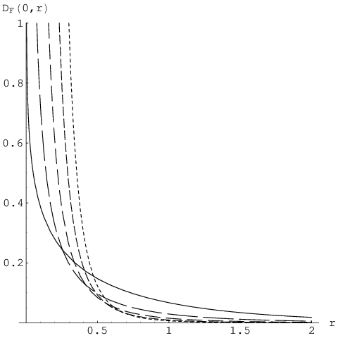
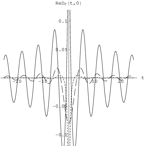
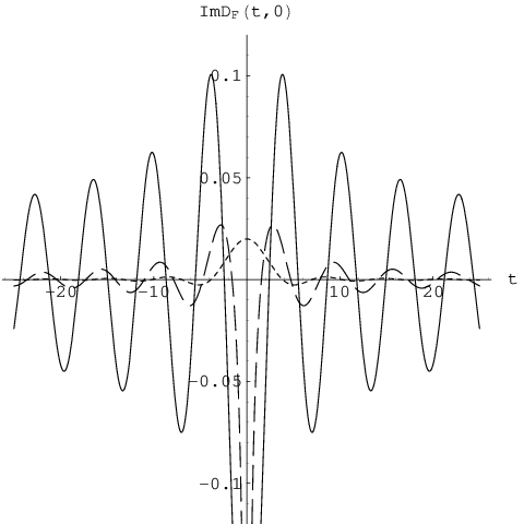
it can be easily verified that if the spatial dimension is taken to be $D=1,2$ , eq.(31) will reduce to eqs.(13),(18), respectively. Therefore, in the following we will use eq.(31) to describe the scalar Feynman propagator in $(D+1)$ -dimensional spacetime for $D\geq 1$ . The shapes of the scalar Feynman propagators with spacelike or timelike separations in different dimensional spacetime are shown in Figs.1 and 2, respectively. The figures exhibit that in any dimensional spacetime, the spacelike propagation amplitude is dominated by the exponential decay, while the timelike propagation amplitude behaves as the damped oscillation; and in both cases the more dimension of spacetime, the more rapidly the propagation amplitude decreases.

Refer to caption — Figure 1: The scalar Feynman propagator $D_{F}(0,r)$ with spacelike separation $r$ in $(D+1)$ -dimensional spacetime, where we have set the mass parameter $m=1$ ; and the solid-line corresponds to $D=1$ , while the dashed-lines, from long to short, correspond to $D=2,3,4,5$ , respectively.

III Feynman propagator of Dirac Theory

In this section, let us calculate the analytic formula of the Feynman propagator in position space of a free Dirac spinor field in $(D+1)$ -dimensional spacetime. Since we have obtained the exact expression of the scalar Feynman propagator in any dimensional spacetime, eq.(31), it is straightforward to get the expression of the spinor Feynman propagator by means of the relation $S_{F}(x)=(i\not{\partial}+m)D_{F}(x)$ . The result we obtain is

$\displaystyle S_{F}(x)$	$\displaystyle=$	$\displaystyle\theta(x^{2})\frac{(-i)^{D-1}m^{\frac{D+1}{2}}\not{x}}{2^{\frac{D+5}{2}}\pi^{\frac{D-1}{2}}(x^{2}-i\epsilon)^{\frac{D+1}{4}}}\bigg[H_{\frac{D-3}{2}}^{(2)}(m\sqrt{x^{2}-i\epsilon})-H_{\frac{D+1}{2}}^{(2)}(m\sqrt{x^{2}-i\epsilon})\bigg]$	(34)
		$\displaystyle+\theta(-x^{2})\frac{im^{\frac{D+1}{2}}\not{x}}{2^{\frac{D+3}{2}}\pi^{\frac{D+1}{2}}(-x^{2}+i\epsilon)^{\frac{D+1}{4}}}\bigg[K_{\frac{D-3}{2}}(m\sqrt{-x^{2}+i\epsilon})+K_{\frac{D+1}{2}}(m\sqrt{-x^{2}+i\epsilon})\bigg]$
		$\displaystyle-\frac{(D-1)}{2}\frac{i\not{x}}{x^{2}-i\epsilon}D_{F}(x)+mD_{F}(x)$

where $\not{x}\equiv\gamma^{\mu}x_{\mu}$ , and where we have used the following recurrence relations of the Hankel function $H_{\nu}^{(2)}(x)$ and the modified Bessel function $K_{\nu}(x)$ :

	$\displaystyle\frac{d}{dx}H_{\nu}^{(2)}(x)=\frac{1}{2}\big[H_{\nu-1}^{(2)}(x)-H_{\nu+1}^{(2)}(x)\big]$		(35)
	$\displaystyle\frac{d}{dx}K_{\nu}(x)=-\frac{1}{2}\big[K_{\nu-1}(x)+K_{\nu+1}(x)\big]$		(36)

In particular, when the spatial dimension $D=3$ , eq.(34) becomes

$\displaystyle S_{F}(x)$	$\displaystyle=$	$\displaystyle-\theta(x^{2})\frac{m^{2}\not{x}}{16\pi(x^{2}-i\epsilon)}\bigg[H_{0}^{(2)}(m\sqrt{x^{2}-i\epsilon})-H_{2}^{(2)}(m\sqrt{x^{2}-i\epsilon})\bigg]$	(37)
		$\displaystyle+\theta(-x^{2})\frac{im^{2}\not{x}}{8\pi^{2}(-x^{2}+i\epsilon)}\bigg[K_{0}(m\sqrt{-x^{2}+i\epsilon})+K_{2}(m\sqrt{-x^{2}+i\epsilon})\bigg]$
		$\displaystyle-\frac{i\not{x}}{x^{2}-i\epsilon}D_{F}(x)+mD_{F}(x)$

which is a little different from the results of Ref.[1], besides the less important factor of $i$ owing to the convention that $D_{F}(x)$ here equals to $i\Delta_{F}(x)$ there. The essential difference between our results and those of Ref.[1] lies in that there is an additional term multiplied by $\delta(x^{2})$ in that book, which is proportional to eq.(34) in page 80 of Ref.[1]. However, we find that this term is redundant, since its proportional factor can be shown to vanish as follows:

	$\displaystyle\hskip-14.22636pt\lim_{x^{2}\to 0}\bigg[\frac{1}{\sqrt{x^{2}-i\epsilon}}H_{1}^{(2)}(m\sqrt{x^{2}-i\epsilon})-\frac{i}{\sqrt{-x^{2}+i\epsilon}}H_{1}^{(2)}(-im\sqrt{-x^{2}+i\epsilon})\bigg]$	(38)
$\displaystyle\sim$	$\displaystyle\frac{1}{\sqrt{x^{2}-i\epsilon}}\frac{i}{\pi}\frac{2}{m\sqrt{x^{2}-i\epsilon}}-\frac{i}{\sqrt{-x^{2}+i\epsilon}}\frac{i}{\pi}\frac{2}{(-im\sqrt{-x^{2}+i\epsilon})}$
$\displaystyle=$	$\displaystyle\frac{2i}{m\pi(x^{2}-i\epsilon)}+\frac{2i}{m\pi(-x^{2}+i\epsilon)}$
$\displaystyle=$	$\displaystyle 0$

The reason why the authors of Ref.[1] regarded the above term as to be nonzero may come from that they had taken both $x^{2}$ and $-x^{2}$ to be the absolute value $|x^{2}|$ simultaneously in their calculation. However, it is obviously impossible that both $x^{2}$ and $-x^{2}$ were equal to $|x^{2}|$ , even if $x^{2}\to 0$ , because $x^{2}$ can only be approaching zero from either of the positive or the negative axis direction, that is, in any case $x^{2}$ and $-x^{2}$ always have opposite signs even if they are infinitesimal.

Moreover, from eq.(34) together with eq.(31), we obtain an interesting recurrence relation for the spinor Feynman propagator in $(D+1)$ -dimensional spacetime and the scalar Feynman propagators in $(D-1)$ -, $(D+1)$ - and $(D+3)$ -dimensional spacetimes as follows

\displaystyle S_{F}^{(D+1)}(x)=\bigg(-\frac{i\not{x}}{x^{2}-i\epsilon}+m\bigg)D_{F}^{(D+1)}(x)-\frac{im^{2}\not{x}}{4\pi(x^{2}-i\epsilon)}D_{F}^{(D-1)}(x)+i\pi\not{x}D_{F}^{(D+3)}(x)

(39)

where the superscripts denote the spacetime dimensions of the respective physical quantities. The above relation essentially stems from the facts that the Feynman propagator in any dimensional spacetime can be expressed in terms of Bessel and modified Bessel functions, which has been proved in this paper. And it exhibits that the free Dirac theory and the free Klein-Gordon theories in alternate-successive dimensional spacetimes might be related to each other.

IV Conclusions

In this paper, we have pointed out and corrected an error of the results of previous works on the analytic expression of the Feynman propagator in position space of a Dirac spinor in $(3+1)$ -dimensional spacetime, and we have derived the generalized analytic formulas of both the scalar Feynman propagator and the spinor Feynman propagator in position space in any $(D+1)$ -dimensional spacetime. The method we have used in this paper is different from that used in Ref.[1]. And the result we have obtained shows that the analytic formula of the Feynman propagator in position space can be also expressed in terms of Hankel functions of second kind and Modified Bessel functions in a general $(D+1)$ -dimensional spacetime, just like the known case in $(3+1)$ -dimensional spacetime. From the obtained results, at the end we have found an interesting recurrence relation among the spinor Feynman propagator in $(D+1)$ -dimensional spacetime and the scalar Feynman propagators in $(D+1)$ -, $(D-1)$ - and $(D+3)$ -dimensional spacetimes.

Acknowledgements.

We would like to thank Profs. Qing Wang, Zhan Xu, Qiong-Gui Lin, and Nai-Ben Huang for helpful discussions. This work is supported by the National Natural Science Foundation of China, and Sun Yet-Sen University Science Foundation.

References

[1] W. Greiner and J. Reinhardt, Quantum Electrodynamics, Springer (1992).
[2] B. S. DeWitt, Dynamical theory of groups and fields, Gordon & Breach, New York (1965).
[3] M. E. Peskin and D. V. Schroeder, An Introduction To Quantum Field Theory, Addison-Wesley (1995).
[4] K. Huang, Quantum field theory: From operators to path integrals, Wiley (1998).
[5] A. Zee, Quantum field theory in a nutshell, Princeton Univ. Pr. (2003).
[6] J. D. Bekenstein and L. Parker, Phys. Rev. D 23, 2850 (1981).
[7] D. W. McKay and H. J. Munczek, Phys. Rev. D 55, 2455 (1997) [arXiv:hep-th/9607075].
[8] F. Antonsen and K. Bormann, arXiv:hep-th/9608141.
[9] A. Di Sessa, Phys. Rev. D 9, 2926 (1974).
[10] M. Gutzwiller, Phys. Stat. Sol. B 237, 39 (2003).
[11] I. S. Gradshteyn, I. M. Ryzhik, Tables of Integrals, Series, and Products (trans. and ed. by Alan Jeffrey), Academic Press, Orlando, Florida (1980).