Hunting for the strangeness content of the nucleon

Many nucleon structure observables require the calculation of disconnected quark line diagrams for which all-to-all propagator techniques are needed. Here we present first results of an ongoing project to calculate the strangeness contribution to the spin of the nucleon $\Delta s$ as well as the scalar strangeness content of the nucleon $\langle N|\bar{s}s|N\rangle$, using improved stochastic methods.

The spin of the nucleon can be factorized into a quark spin contribution $\Delta\Sigma$, a quark angular momentum contribution $L_{q}$ and a gluonic contribution (spin and angular momentum) $\Delta G$:

In the naïve $SU(6)$ quark model, $\Delta\Sigma=1$, with vanishing angular momentum and gluon contributions. In this case sea quark contributions will be absent too and therefore there will be no strangeness contribution $\Delta s$ in the factorisation,

where in our notation $\Delta q$ contains both, the spin of the quarks $q$ and of the antiquarks $\bar{q}$. Experimentally $\Delta s$ is usually obtained by integrating the strangeness contribution to the spin structure function $g_{1}$ over momentum transfers $x$. The integral over the range in which data exists ($x\gtrsim 0.004$) typically agrees with zero which means that a non-zero result relies on the unprobed very small-$x$ region and is model dependent. Recent Hermes analysis [1] yields $\Delta s=-0.085(13)(8)(9)$ at a renormalization scale $\mu^{2}=5\,$GeV² in the $\overline{MS}$ scheme while our (as yet unrenormalized) results suggest $|\Delta s|<0.01$.

The scalar strangeness density is not directly accessible in experiment but plays a rôle in models of nuclear structure. It is also of phenomenological interest since, assuming that heavy flavours are strongly suppressed, the dominant coupling of the Higgs particle to the nucleon will be accompanied by this scalar matrix element.

We will first discuss our methods, then the error reduction achieved in our present lattice setup and finally we present results on the two matrix elements, before concluding.

We denote the lattice spacing by $a$ and the lattice Dirac matrix by $M={\mathbb{1}}-\kappa\!\not\!\!D$. Disconnected quark line contributions require all-to-all propagators $M^{-1}_{ji}$ where the multi-index $i=(x,\alpha,a)$ runs over all colours $a=1,2,3$, spinor indices $\alpha=1,\ldots,4$ and spacetime sites $x\in V$. Note that in our particular application it is natural and sufficient to restrict $x$ to a given timeslice. Exact methods to obtain $M^{-1}$ are unfeasible in terms of computer time and memory since $12V$ solver applications are required. Employing stochastic methods [2], this factor can be substituted by the number of estimates $L\ll 12V$: in a first step a set of Dirac noise vectors $\{|\eta_{\ell}\rangle:\ell=1,\ldots,L\}$ is generated where the $12V$ complex colour-spinor-site components are filled with $({\mathbb{Z}}_{2}\otimes i\,{\mathbb{Z}}_{2})/\sqrt{2}$ uncorrelated random numbers [3]. These have the following properties:

We will also employ the short-hand notation $\overline{|\cdot\rangle\langle\cdot|}=\overline{|\cdot\rangle\langle\cdot|}_{L}$. We use the conjugate gradient algorithm with even/odd preconditioning to obtain the solutions $|s_{\ell}\rangle$ of the sparse linear problems,

From these one can construct an unbiased estimate of $M^{-1}$:

Due to the difference between $E(M^{-1})$ and $M^{-1}$ above, any fermionic observable $A$ can only be estimated up to a stochastic error $\Delta_{\rm stoch}A=\mathcal{O}(1/\sqrt{L})$ on a given configuration. We define the configuration average $\langle\cdot\rangle_{c}$ over $n_{\rm conf}$ uncorrelated configurations and normalize this appropriately:

For large $L$ and $n_{\rm conf}$ this will scale like $\sigma_{A,\rm stoch}^{2}\propto(Ln_{\rm conf})^{-1}$. We also define the gauge error $\sigma^{2}_{A,\rm gauge}\propto n_{\rm conf}^{-1}$ as the variation of the estimates of $A$ over gauge configurations. This will be minimized at fixed $n_{\rm conf}$ if $A$ is calculated exactly. In general the gauge error is limited by,

If $\sigma^{2}_{A,\rm stoch}\simeq\sigma^{2}_{A,\rm gauge}$ then obviously it is worthwhile to improve the quality of the estimates while if $\sigma^{2}_{A,\rm stoch}\ll\sigma^{2}_{A,\rm gauge}$ then precision can only be gained by increasing $n_{\rm conf}$, possibly reducing $L$ to save computer time since the same $n_{\rm conf}^{-1}$ scaling enters both sides of the inequality.

In our calculation of $\Delta s$ the stochastic error initially was dominant. Hence we combined several variance reduction techniques to reduce this:

• •

  partitioning (also coined dilution) [4]: we only set $|\eta_{\ell}\rangle\neq 0$ on one timeslice. This removes some of the (larger) off-diagonal noise elements, see eq. (5), and reduces the variance.

• •

  hopping parameter expansion (HPE) [5]: the first few terms of the hopping parameter expansion of $\mbox{Tr}(\Gamma M^{-1})=\mbox{Tr}[\Gamma(\mathbb{1}-\kappa\!\not\!\!D)^{-1}]$ vanish identically but still contribute to the noise. For the Wilson action, $\mathrm{Tr}(\Gamma M^{-1})=\mathrm{Tr}(\Gamma\kappa^{n}\!\not\!\!D^{n}{M}^{-1})$ for $n=4,8$, depending on $\Gamma$, where for $\Gamma={\mathbb{1}}$ one can easily calculate and correct for the zero-order difference.

• •

  truncated solver method (TSM) [6]: calculate approximate solutions $|s_{n_{\rm t},\ell}\rangle$ after $n_{\rm t}$ solver iterations (before convergence), and estimate the difference stochastically to obtain an unbiased estimate of $M^{-1}$:

  $$\mathrm{E}(M^{-1})=\overline{|s_{n_{\rm t}}\rangle\langle\eta|}_{L_{1}}+\overline{(|s\rangle-|s_{n_{\rm t}}\rangle)\langle\eta|}_{L_{2}}\quad\mbox{where}\quad L_{2}\ll L_{1}\,.$$

• •

  Truncated eigenmode approach (TEA) [7, 8]: calculate the $n_{\rm ev}$ lowest eigenvalues and eigenvectors of $\mathrm{Q}=\gamma_{5}M=Q^{\dagger}$, $\mathrm{Q}^{-1}=\mathrm{Q}^{-1}_{\perp}+\sum_{i=1}^{n_{\rm ev}}|u_{i}\rangle q_{i}^{-1}\langle u_{i}|$, and stochastically estimate the complement $\mathrm{Q}^{-1}_{\perp}$ (with deflation included for free).

Our exploratory calculations are performed on $V=16^{3}\times 32$ configurations of $n_{f}\approx 2+1$ rooted stout-link improved staggered quarks with a Symanzik improved gauge action. These were provided by the Wuppertal group. The lattice spacing is fairly coarse, $a^{-1}\approx 1.55$ GeV, and the spatial dimension is around $2$ fm [9]. We used the Wilson action for our valence quarks and currents with $\kappa=0.166$, $0.1675$ and $0.1684$, corresponding to pseudoscalar masses of about $600$, $450$ and $300$ MeV respectively. The analysis was performed on 326 configurations at $\kappa_{\rm loop}=0.166$, 167 configurations at $\kappa_{\rm loop}=0.1675$ and $152$ configurations at $\kappa_{\rm loop}=0.1684$, where $\kappa_{\rm loop}$ refers to the $\kappa$ value of the disconnected loop. Throughout we used a modified version of the Chroma code [10].

On each configuration the disconnected loop was calculated using the stochastic variance reduction techniques detailed above (the TEA was only used at $\kappa_{\rm loop}=0.1684$, where $20$ eigenvalues were calculated). We investigate the reduction in computer time, using optimized stochastic estimates, relative to those without any improvement techniques applied (except for time partitioning). We state all costs in terms of the average real computer time required on a Pentium 4 PC for one solver application (unimproved estimate), where we account for all overheads of the improvement methods.

Results for the configuration averages of the loops $\mathrm{Tr}(\Gamma_{\rm loop}\mathrm{M}^{-1})$ are given in table 1. The gauge errors $\sigma_{\rm gauge}$ (that also depend on the stochastic noise) are displayed in brackets after the loop averages. These can be compared to the purely stochastic errors $\sigma_{\rm stoch}$, defined in eq. (6). The deflation at $\kappa_{\rm loop}=0.1684$ where we apply TEA accelerates the solver but time is required for the eigenvector set-up. In our implementation the cost of solving for about 90 undeflated right hand sides equals that of 90 deflated ones (including this overhead). This is why in this case we do not display results obtained at the lower cost values.

For $\mathrm{Tr}(\frac{1}{3}\sum_{j}\gamma_{j}\gamma_{5}\mathrm{M}^{-1})$ the stochastic error dominates over the gauge error unless $L$ is chosen ridiculously large or variance reduction techniques are applied. Using these techniques the error is brought under control to the extent that we only need to invest the computer time equivalent of roughly 100 unimproved stochastic estimates to achieve $\sigma_{\rm stoch}<\frac{1}{2}\sigma_{\rm gauge}$. In particular, we find a reduction in $\sigma_{\rm stoch}^{2}$ (which is proportional to the amount of computer time required) of approximately 25–30 for $\kappa_{\rm loop}=0.166$ and $0.1684$. A smaller gain is obtained for the intermediate $\kappa_{\rm loop}=0.1675$ which may benefit from using the TEA approach. For $\mathrm{Tr}(\mathbb{1}\mathrm{M}^{-1})$ the situation is reversed and the gauge error clearly dominates over the stochastic error: apart from possibly the heaviest $\kappa_{\rm loop}$ there is no advantage in using variance reduction techniques.

The matrix elements,

and $\langle N|\bar{q}q|N\rangle$ are extracted from the ratios of three-point functions to two-point functions (at zero momentum):

where $\Gamma_{\rm 2pt}=\Gamma_{\rm unpol}=(1+\gamma_{4})/2$ and $\Gamma_{\rm loop}=\mathbb{1}$ for $\langle N|\bar{q}q|N\rangle$ and $\Gamma_{\rm 2pt}=i\gamma_{j}\gamma_{5}(1+\gamma_{4})/2$ and $\Gamma_{\rm loop}=\gamma_{j}\gamma_{5}$ for $\Delta q$, where we average over $j=1,2,3$. Note that for $q=u,d$ there is an additional connected contribution $R^{\rm con}$, which we have not calculated. We combine the three $\kappa_{\rm loop}$ values with $\kappa_{\rm 2pt}=0.166$ and 0.1675. In the limit of large times, $t_{f}\gg t\gg t_{0}$,

We optimized the nucleon creation and annihilation operators using Wuppertal smearing with spatial APE-smeared parallel transporters [8]. The effective mass plot of figure 1 illustrates ground state dominance from a time $t=3a\approx 0.38\,$fm onwards. The same holds for $\kappa_{\rm 2pt}=0.1675.$ Hence we place the source at $t_{0}=0$, the current insertion at $t=3a$ and destroy the nucleon at $t_{f}\geq 4a$. The result on the right of figure 1 does not depend on $t_{f}$, even for $t_{f}<6a$, indicating that indeed with the chosen temporal separations we effectively realize the large-$t$ limit. In table 2 we display the results for $\Delta q^{\rm dis}$ at the symmetric point $t_{f}=6a\approx 0.76$ fm: our methods enable us to reduce the squared errors by factors ranging from 5.5 to 11 at the fixed computational cost of 100 solver applications (in addition to calculating the two-point function). This falls somewhat short of the gains that we achieved in table 1 for the loops alone since now there are additional sources of gauge error. These we attempt to address in the near future.

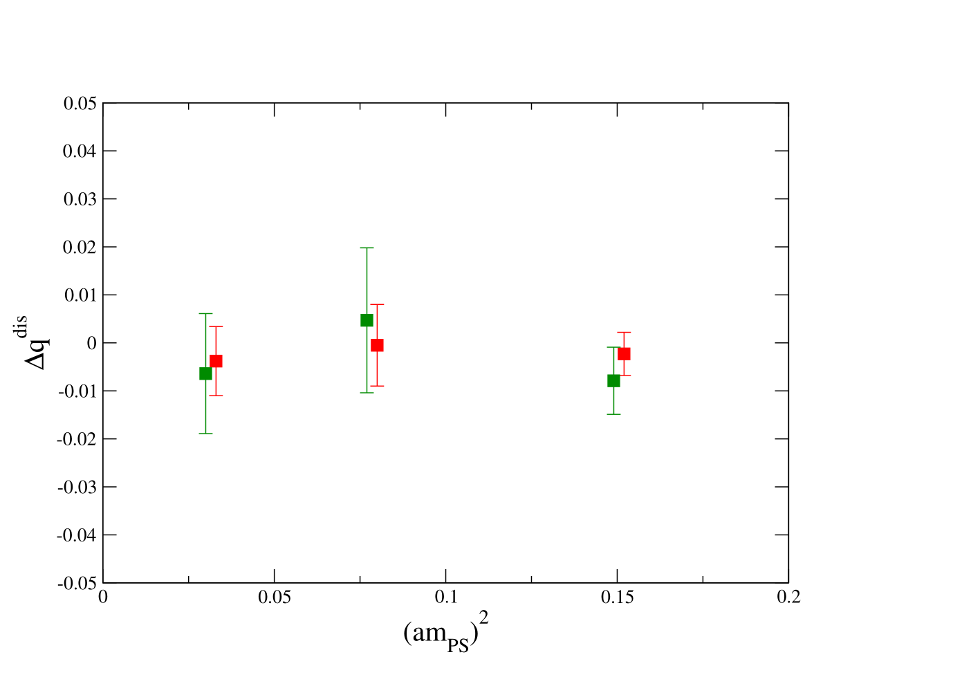
In figure 2 we display our results for the two matrix elements where we obtained $\langle N|\bar{q}q|N\rangle^{\rm dis}$ at the cost of 12 solver applications per configuration and $\Delta q^{\rm dis}$ at the cost of 100 applications, in addition to the 12 applications that are necessary to calculate the two point functions. In neither case do we observe any significant dependence on the valence quark mass, varying this from $m_{\pi}\approx 600$ MeV down to 450 MeV, or on the loop quark mass, reducing $m_{\pi}\approx 600$ MeV ($\simeq$ strange quark mass) to $m_{\pi}\approx 300$ MeV. We find $|\Delta s|<0.011$ at the heavier proton mass and $|\Delta s|<0.022$ at the lighter mass value with 95 % confidence level while the scalar matrix element appears to be somewhat larger than one. Note however that the lattice results presented here are unrenormalized.

In the near future we will further reduce the quark masses and the statistical errors, in particular also of the scalar density, by refining our methods. We will also move to non-perturbatively improved Wilson sea quarks, allowing us to renormalize the results and to obtain a well-defined continuum limit.