Second order hydrodynamic coefficients from kinetic theory

Mark Abraao York and Guy D. Moore Affiliation: McGill University Dept. of Physics, 3600 rue University, Montréal QC H3A 2T8 Canada

October 2008: v2 February 2009

Abstract

In a relativistic setting, hydrodynamic calculations which include shear viscosity (which is first order in an expansion in gradients of the flow velocity) are unstable and acausal unless they also include terms to second order in gradients. To date such terms have only been computed in supersymmetric ${\cal N}{=}4$ Super-Yang-Mills theory at infinite coupling. Here we compute these second-order hydrodynamic coefficients in weakly coupled QCD, perturbatively to leading order in the QCD coupling, using kinetic theory. We also compute them in QED and scalar $\lambda\phi^{4}$ theory.

I Introduction and results

Recently the Relativistic Heavy Ion Collider (RHIC) at Brookhaven has successfully created the quark-gluon plasma. Measurements of elliptic flow [1] indicate collective fluid behavior which implies a startlingly low viscosity [2]. Actually, measured in Poise the viscosity is enormously large; but this is expected of such a hot and dense system. It has recently been argued [3] that viscosity naturally scales with entropy density. Their ratio $\eta/s$ is dimensionless [in natural units, used throughout; restoring $\hbar$ and $c$ , it has units of $\hbar$ ] and is conjectured to be bounded below by $\eta/s\geq 1/4\pi$ (see however [4]).

It is believed that the quark-gluon plasma created at RHIC displays a viscosity relatively close to this bound. But it is important to quantify this by comparing experimental results for elliptic flow spectra to the predictions of viscous hydrodynamics simulations. Several groups are engaged in this [5, 6, 7, 8, 9], but it is not as simple as adding a viscosity term to the ideal hydrodynamical equations. Indeed, it has been known for decades that relativistic Navier-Stokes equations are acausal and unstable [10, 11, 12].¹¹ 1 The easy way to understand this is to note that Navier-Stokes equations are Euler equations plus a momentum-diffusion term, with the viscosity as the momentum-diffusion coefficient. But diffusion equations possess infinite propagation speeds for information, which is problematic in a relativistic setting.

Viscosity is just the first-order term in a gradient-expansion of corrections to ideal Eulerian hydrodynamics; Israel and Stewart showed 30 years ago that the stability problems could be repaired by the inclusion of certain second-order terms as well [11]. This is the guiding philosophy for most recent viscous hydrodynamics studies of the quark-gluon plasma.

However, once one allows for some second-order in gradients terms, it seems wise to at least consider all second-order terms which could appear and to make an estimate of their size relative to the shear viscosity. This program was begun recently by Baier et al [13], who showed that, with the additional assumption of conformal invariance (a good approximation in QCD if the temperature is well above the QCD transition/crossover temperature of $\sim 170$ MeV), there are five second-order coefficients, one of which is only relevant in curved space.

It would be valuable to have a reasonable estimate of the size of these second-order coefficients, or an estimate of how they scale with the shear viscosity. Baier et al and the Tata group [14] have given one estimate, by evaluating the five coefficients in a toy model for QCD, strongly coupled ${\cal N}{=}4$ Super-Yang-Mills theory (see also [15]). Here we evaluate the five second-order coefficients in QCD to leading order in the weak coupling expansion, using kinetic theory. In the thermal field theory setting the coupling expansion is not believed to converge very well (see for instance [16]), so weakly coupled QCD should also be viewed as a “toy model” for QCD at realistic couplings. However we hope that the combined insight from the two “toy models” give a reasonable idea of the expected scaling of these second-order coefficients relative to shear viscosity.

We evaluate the flat-space coefficients in Section II and the curved-space coefficient in Section III. We then give an extensive discussion, in Section IV, of the physical interpretation of each second-order transport coefficient, and some interesting physical issues which arise in their computation. Certain technical details involving nonlinear corrections arising through plasma screening are postponed to Appendix A. But we will finish introducing the problem and present the main results and conclusions here.

All hydrodynamic approaches are based on stress-energy conservation,

\partial_{\mu}T^{\mu\nu}=0\,,

(1)

which is 4 equations for 10 unknowns.²² 2 Here we only consider systems with vanishing densities of other conserved charges such as baryon number. The other 6 equations are established by gradient expanding the form of $T^{\mu\nu}$ about its equilibrium form. In the absence of nonzero conserved charge densities (which we will assume henceforward), in equilibrium³³ 3 We use the $[{-}{+}{+}{+}]$ metric convention

T^{\mu\nu}=(\epsilon+P)u^{\mu}u^{\nu}+Pg^{\mu\nu},\qquad u_{\mu}u^{\mu}=-1\;\;\mbox{with}\;\;u^{0}>0\,,\quad P=P(\epsilon)\,.

(2)

This determines $T^{\mu\nu}$ in terms of 4 unknowns, the energy density $\epsilon$ and 3 components of the flow 4-vector $u^{\mu}$ . However, if $\epsilon,u^{\mu}$ vary in space and time⁴⁴ 4 It is also necessary to choose some convention defining $\epsilon$ and $u$ . We take the Landau-Lifshitz convention that $u_{\mu}T^{\mu\nu}\propto u^{\nu}$ and $\epsilon\equiv u_{\mu}u_{\nu}T^{\mu\nu}$ . then we expect corrections to Eq. (2). For slowly varying $\epsilon$ and $u^{\mu}$ the corrections can be expanded in gradients of these quantities. At first order in gradients and in a conformal theory, defining the rest-frame spatial projector

\Delta^{\mu\nu}\equiv g^{\mu\nu}+u^{\mu}u^{\nu}

(3)

and working in flat space (so $\nabla_{\mu}=\partial_{\mu}$ and $g_{\mu\nu}=\eta_{\mu\nu}$ ), the only possible combination is

T^{\mu\nu}=T^{\mu\nu}_{\rm eq}+\Pi^{\mu\nu}\,,\quad\Pi^{\mu\nu}_{\rm 1\;order}=-\eta\sigma^{\mu\nu}\,,\quad\sigma^{\mu\nu}\equiv\Delta^{\mu\alpha}\Delta^{\nu\beta}\left(\partial_{\alpha}u_{\beta}+\partial_{\beta}u_{\alpha}-\frac{2}{3}g_{\alpha\beta}\Delta^{\gamma\delta}\partial_{\gamma}u_{\delta}\right)\,.

(4)

Here $\eta=\eta(\epsilon)$ is the shear viscosity, defined as the coefficient multiplying the traceless part of the transverse symmetrized shear flow tensor. The bulk viscosity, defined as the proportionality constant for the pure-trace part $\Pi^{\mu\nu}\propto\Delta^{\mu\nu}\Delta_{\alpha\beta}\partial^{\alpha}u^{\beta}$ , vanishes in a conformal theory.

Baier et al ([13] Eq. (3.11)) show that there are four possible second-order flat-space terms:

$\displaystyle\hskip-14.45377pt\Pi^{\mu\nu}_{\rm 2\;order}$	$\displaystyle=$	$\displaystyle\eta\tau_{\Pi}\left[u^{\alpha}\partial_{\alpha}\sigma^{\mu\nu}+\frac{1}{3}\sigma^{\mu\nu}\partial_{\alpha}u^{\alpha}\right]+\lambda_{1}\left[\sigma^{\mu}_{\alpha}\sigma^{\nu\alpha}-\frac{1}{3}\Delta^{\mu\nu}\sigma_{\alpha\beta}\sigma^{\alpha\beta}\right]$	(5)
		$\displaystyle+\lambda_{2}\left[\frac{1}{2}(\sigma^{\mu}_{\alpha}\Omega^{\nu\alpha}+\sigma^{\nu}_{\alpha}\Omega^{\mu\alpha})-\frac{1}{3}\Delta^{\mu\nu}\sigma_{\alpha\beta}\Omega^{\alpha\beta}\right]+\lambda_{3}\left[\Omega^{\mu}{}_{\alpha}\Omega^{\nu\alpha}-\frac{1}{3}\Delta^{\mu\nu}\Omega_{\alpha\beta}\Omega^{\alpha\beta}\right]\,,$	(5)
$\displaystyle\Omega_{\mu\nu}$	$\displaystyle\equiv$	$\displaystyle\frac{1}{2}\Delta_{\mu\alpha}\Delta_{\nu\beta}(\partial^{\alpha}u^{\beta}-\partial^{\beta}u^{\alpha})\;\mbox{ [vorticity]}\,.$

Physically, $\tau_{\Pi}$ tells how quickly the anisotropic stress $\Pi^{\mu\nu}$ relaxes to the leading-order form $-\eta\sigma^{\mu\nu}$ , if it starts out with a different value. The parameter $\lambda_{1}$ tells how nonlinear the viscous effects are; $\lambda_{2,3}$ are similar but for systems with nonzero vorticity. An additional term $\kappa(R^{\mu\nu}+\ldots)$ is possible in curved space. It is these quantities we want to determine in weakly coupled QCD. We describe their physical significance in more detail in Section IV.

Expressing $\eta$ in terms of the dimensionless ratio $\eta/s$ disguises the fact that $\eta$ really reports a time scale, roughly speaking the equilibration time of the system. The gradient expansion of Eq. (4), Eq. (5) is an expansion in this time scale divided by the scale of spacetime variation of the system. To identify the time scale, divide $\eta$ not by the entropy density but by the enthalpy density: $\frac{\eta}{\epsilon+P}\propto\frac{1}{T}$ , a time. In ${\cal N}{=}4$ SYM theory at strong coupling the ratio is $\frac{\eta}{\epsilon+P}=\frac{1}{4\pi T}$ . In weakly coupled QCD it is parametrically $\frac{\eta}{\epsilon+P}\sim\frac{1}{g^{4}T\ln(1/g)}$ [17, 18, 19, 20]. Similarly, the ratio of each second order coefficient to $(\epsilon{+}P)$ yields the square of a time. It is natural to expect $\frac{\lambda_{1}}{\epsilon+P}\sim(\frac{\eta}{\epsilon+P})^{2}$ . The numerical value of the ratio $\frac{\lambda_{1}}{(\epsilon+P)}/(\frac{\eta}{\epsilon+P})^{2}=\frac{(\epsilon+P)\lambda_{1}}{\eta^{2}}$ is a convenient way to express the relative size of the second-order coefficient $\lambda_{1}$ to $\eta$ . In particular we expect most coupling dependence to cancel in this ratio, which should therefore differ relatively little between weak and realistic coupling.

We find that at weak coupling, at leading order the ratios of second-order to first-order hydrodynamic coefficients are

$\displaystyle\frac{(\epsilon{+}P)\eta\tau_{\Pi}}{\eta^{2}}$	$\displaystyle=$	$\displaystyle\mbox{5.9 to 5.0 (varies with $g$)}\,:\quad 6.10517\mbox{ in }\lambda\phi^{4}\mbox{ theory}\,,$	(6)
$\displaystyle\frac{(\epsilon{+}P)\kappa}{\eta^{2}}$	$\displaystyle=$	$\displaystyle 0\,,$	(7)
$\displaystyle\frac{(\epsilon{+}P)\lambda_{1}}{\eta^{2}}$	$\displaystyle=$	$\displaystyle\mbox{5.2 to 4.1 (varies with $g$)}\,:\quad 6.13264\mbox{ in }\lambda\phi^{4}\mbox{ theory}\,,$	(8)
$\displaystyle\frac{(\epsilon{+}P)\lambda_{2}}{\eta^{2}}$	$\displaystyle=$	$\displaystyle-2\frac{(\epsilon{+}P)\eta\tau_{\Pi}}{\eta^{2}}\,,$	(9)
$\displaystyle\frac{(\epsilon{+}P)\lambda_{3}}{\eta^{2}}$	$\displaystyle=$	$\displaystyle 0\,.$	(10)

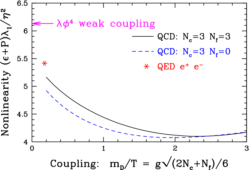
The detailed coupling dependence of the two independent nonzero coefficients, $\eta\tau_{\Pi}$ and $\lambda_{1}$ , are shown in Fig. 1 and Fig. 2. These figures display results for QCD with either 0 or 3 flavors of quarks, and for $e^{+}e^{-}$ QED at realistic coupling [ $\frac{(\epsilon{+}P)\tau_{\Pi}}{\eta}=5.9664$ and $\frac{(\epsilon{+}P)\lambda_{1}}{\eta^{2}}=5.4156$ ] as well as indicating the results for weakly coupled $\lambda\phi^{4}$ theory. We have expressed the results in terms of $m_{\rm D}/T$ the ratio of Debye screening length and temperature, which proves convenient computationally and is the right quantity for parametrizing whether a coupling is strong or weak at finite temperature. Numerically, $\alpha_{\rm s}=(2/12\pi)(m_{\rm D}/T)^{2}$ in 3-flavor QCD, $\alpha_{\rm s}=(1/4\pi)(m_{\rm D}/T)^{2}$ in 0-flavor QCD, and $\alpha_{{}_{\rm EM}}=(3/4\pi)(m_{\rm D}/T)^{2}$ in 1-flavor QED. Further discussion on these results and their physical meaning is postponed to the discussion section, Section IV.

We find an exact relation $\lambda_{2}/\eta\tau_{\Pi}=-2$ , in agreement with [21]. This relation is an automatic consequence of ultra-relativistic (conformal) kinetic theory. However unlike [21] we do not find $\lambda_{1}=\eta\tau_{\Pi}$ . This is because [21] fixes an Ansatz for the functional form of the departure from equilibrium and drops some contributions arising from the nonlinearity of the collision operator. We discuss this in more detail in what follows. However in practice $\lambda_{1}/\eta\tau_{\Pi}$ is relatively close to 1. We also find that $\kappa=0=\lambda_{3}$ in QCD, in QED, in scalar $\phi^{4}$ theory, and indeed in any conformal theory described by kinetic theory. But this does not mean that these coefficients are strictly zero; it means that they first arise in the perturbative expansion at a higher order than $\eta\tau_{\Pi}$ and $\lambda_{1}$ do. That is, $\lambda_{1}\propto T^{2}/(g^{8}\ln^{2}(1/g))+{\cal O}(T^{2}/g^{6})$ ; but $\kappa$ may only scale as, say, $T^{2}/g^{4}$ and it is therefore zero in a leading-order evaluation, which only finds the $\propto T^{2}/g^{8}$ coefficients. This is discussed more in Section III.

Refer to caption — Figure 1: Coupling dependence of the ratio $(\epsilon{+}P)\tau_{\Pi}/\eta$ . This ratio compares the relaxation time scale for $\Pi_{\mu\nu}$ , $\tau_{\Pi}$ , to the time scale implied by the viscosity $\eta$ .

For comparison, combining the results of [13] and [14], the same coefficients in ${\cal N}{=}4$ SYM theory are

$\displaystyle\frac{(\epsilon{+}P)\eta\tau_{\Pi}}{\eta^{2}}$	$\displaystyle=$	$\displaystyle 4-2\ln(2)\simeq 2.6137\,,$	(11)
$\displaystyle\frac{(\epsilon{+}P)\kappa}{\eta^{2}}$	$\displaystyle=$	$\displaystyle 4\,,$	(12)
$\displaystyle\frac{(\epsilon{+}P)\lambda_{1}}{\eta^{2}}$	$\displaystyle=$	$\displaystyle 2\,,$	(13)
$\displaystyle\frac{(\epsilon{+}P)\lambda_{2}}{\eta^{2}}$	$\displaystyle=$	$\displaystyle-4\ln(2)\simeq-2.7726\,,$	(14)
$\displaystyle\frac{(\epsilon{+}P)\lambda_{3}}{\eta^{2}}$	$\displaystyle=$	$\displaystyle 0\,.$	(15)

After scaling by the viscosity as described, the second-order coefficient $\eta\tau_{\Pi}$ is about twice as large at weak coupling as at ultra-strong coupling. The relation between $\eta\tau_{\Pi}$ and $\lambda_{2}$ valid at weak coupling is violated at strong coupling, and the coefficient $\lambda_{1}$ is also about two times larger at weak than at strong coupling. It is reasonable to expect that, in QCD at realistic couplings, the dimensionless ratios will fall between the weak-coupled values and the (generally smaller) ultra-strong coupled SYM values. Certainly we expect the QCD values for these dimensionless ratios to be of the same order of magnitude as what we find in both theories, wherever QCD is relatively close to conformal (starting somewhat above $T_{c}$ ). However given the difference in detail between values in the two theories it is tough to be confident in the exact values for realistic QCD.

II Kinetic theory to second order

II.1 Kinetic theory setup

We will not discuss the derivation of kinetic theory here; for a review see [22, 23, 24, 25, 26]. Kinetic theory can be used when each of several criteria apply:

1.

There are long-lived quasiparticles (spectral functions for relevant fields or composite operators have sharp quasiparticle peaks).
2.

The density matrix is adequately approximated by a Gaussian approximation, that is, by the two-point function. Further, the system varies slowly in space and time, so we may work in terms of a space and momentum dependent distribution function $f^{a}({\bf x},{\bf p})$ . Here $a$ is a label which runs over all quasiparticle types (species, spin, color, particle/antiparticle). (Note that ${\bf x}$ and ${\bf p}$ don’t commute, but if the spatial variation is slow enough then we can neglect the commutator and treat them as continuous, independent variables.)
3.

The quasiparticles dominate the measurables of interest and the dynamics.

All of these criteria hold for weakly coupled relativistic field theories, even gauge theories [25], if we are interested in the transport coefficients which appear in the hydrodynamical description just discussed. The validity of the kinetic approach has been verified (at leading order) by explicit diagrammatic analysis both in scalar field theory [27] and in gauge theory [28, 29, 30].

The kinetic theory description describes the time evolution of the distribution function $f^{a}({\bf x},{\bf p})$ . This is determined by the Boltzmann equation. In covariant notation, it is⁵⁵ 5 We use capital letters $P$ for 4-vectors, boldface ${\bf p}$ for 3-vector components, and $p$ for the magnitude $|{\bf p}|$ of the 3-vector. The collision operator here differs by a factor of $2p^{0}$ from that in [18, 19, 20]. This normalization difference will disappear when we integrate $\int_{p}$ , since this integral carries a factor $1/2p_{0}$ absent in [19, 20]. The overall minus sign on ${\cal C}$ is chosen so that its linearized form acts on the departure from equilibrium $\delta f$ as a positive definite operator. To see the full covariance of the Boltzmann equation, think of $f^{a}(x,{\bf p})$ as a function of 4-momentum $P$ but with support only on the forward light cone, $f^{a}(x,P)=\delta(P^{2})\delta(p^{0})f^{a}(x,{\bf p})$ .

$\displaystyle 2P^{\mu}\partial_{\mu}f^{a}(x,{\bf p})$	$\displaystyle=$	$\displaystyle-{\cal C}[f]\mbox{ ``Collision operator''}$	(16)
	$\displaystyle\equiv$	$\displaystyle-\sum_{a_{i},b_{j}}\frac{1}{n_{i}!n_{j}!}\int_{k_{i},k^{\prime}_{j}}(2\pi)^{4}\delta^{4}\left(P+\sum K_{i}-\sum K^{\prime}_{j}\right)\|{\cal M}\|_{a_{i},b_{j}}^{2}[{\bf p},{\bf k}_{i},{\bf k}^{\prime}_{j}]\times$
		$\displaystyle\quad\qquad\Big(f^{a}({\bf p})\prod_{i,j}f^{a_{i}}({\bf k}_{i})[1{\pm}f^{b_{j}}({\bf k}^{\prime}_{j})]-[1{\pm}f^{a}({\bf p})]\prod_{i,j}[1{\pm}f^{a_{i}}({\bf k}_{i})]f^{b_{j}}({\bf k}^{\prime}_{j})\Big)\,.$

Here we have defined $p^{0}$ in terms of the on-shell condition $p^{0}=E_{p}\equiv\sqrt{{\bf p}^{2}+m^{2}}=p$ (in a conformal theory $m=0$ up to ${\cal O}(g^{2})$ medium corrections, which we will neglect since we seek a leading-order treatment), and we have introduced the shorthand

\int_{k}\equiv\int\frac{d^{3}{\bf k}}{(2\pi)^{3}2k^{0}}=\int\frac{d^{4}K}{(2\pi)^{4}}2\pi\delta(K^{2})\Theta(k^{0})\,.

(17)

The lefthand side of Eq. (16) describes the free propagation of particles; the time rate of change of the occupancy $E\partial_{t}f$ is determined by the particles’ motion $p^{i}$ times the spatial variation of the distribution function $\partial_{i}f(x,p)$ . The righthand side describes the change in occupancy due to collisions, which are approximated as spacetime-local (so all $f$ on the RHS are evaluated at the point $x$ ). The first product of population functions represents the rate at which particles of momentum ${\bf p}$ are scattered out of that momentum state; $[1{\pm}f({\bf k}^{\prime})]$ is a Bose stimulation $(+)$ or Pauli blocking $(-)$ final state factor. The second product of population functions is the rate for the reverse process, producing a particle of momentum ${\bf p}$ . In equilibrium and in the local rest frame, $[1{\pm}f_{\rm eq}(k)]=f(k)e^{k/T}$ and so the two terms cancel by energy conservation, ensuring detailed balance.

The Boltzmann equation rests on several approximations, such as the separation of scales between the distance between collisions ( ${\cal O}(1/g^{2}T)$ in gauge theories) and the physical size of collisions ( ${\cal O}(1/gT)$ ) or deBroglie wavelengths of excitations ( ${\cal O}(1/T)$ ). It is not clear how to incorporate systematic corrections to these approximations. It is also problematic to evaluate the collision operator to high order in the coupling; for instance in QCD we anticipate that nonperturbative magnetic physics causes scatterings suppressed only by $g^{2}$ relative to the dominant $2\leftrightarrow 2$ scattering processes. Indeed, we will shortly encounter (weak) logarithmic dependence on this scale in the second-order calculation performed here. Therefore it is not clear whether or how the kinetic treatment can compute transport coefficients beyond leading order⁶⁶ 6 Note that the first corrections to the calculations we present here actually arise at order $g$ , not $g^{2}$ . However we believe that the ${\cal O}(g)$ corrections can be computed within kinetic theory; indeed this has been done in a few cases [31, 16]. in $g^{2}$ . So we will not try. This excuses us to simplify the collision operator to include only $2\leftrightarrow 2$ and effective $1\leftrightarrow 2$ scattering processes; in QCD the relevant collision terms are presented in [32]. It also means that we can neglect the scale dependence of the QCD coupling (the $\beta$ function). Therefore QCD behaves as a conformal theory,⁷⁷ 7 For simplicity we will consider only massless QCD. and the analysis of Baier et al [13] is relevant.

II.2 Order by order expansion

Our goal is to solve the Boltzmann equation for the case of a near-equilibrium system with slowly varying energy and momentum density $(\epsilon,P^{i})$ , or equivalently their dual variables, the temperature $T$ and flow velocity $u^{i}$ . We write $f(x,{\bf p})$ as a formal series

f(x,{\bf p})=f_{0}+\lambda f_{1}+\lambda^{2}f_{2}+\ldots

(18)

with $\lambda$ a parameter keeping track of the order in derivatives. The lefthand side of the Boltzmann equation, Eq. (16) has an explicit derivative so it starts at ${\cal O}(\lambda)$ . Therefore $f_{0}$ is fixed by the condition ${\cal C}[f_{0}]=0$ . The solution is (note that $u^{\mu}P_{\mu}<0$ ; $\beta\equiv 1/T$ as usual)

f_{0}(x,{\bf p})=(\exp(-\beta u^{\mu}P_{\mu})\mp 1)^{-1}\,,\qquad\beta=\beta(x),\;u^{\mu}=u^{\mu}(x)\,,\;p^{0}=p\,,

(19)

with $\mp=-$ for bosons and $+$ for fermions. At first order we have

2P^{\mu}\partial_{\mu}f_{0}=-{\cal C}_{1}[f_{1}]\,,

(20)

where we use the notation ${\cal C}_{1}$ to mean that ${\cal C}[f]$ is expanded to first order in $f_{1}$ , see Eq. (51). At the second order we will have

2P^{\mu}\partial_{\mu}f_{1}=-{\cal C}_{11}[f_{1}]-{\cal C}_{1;{\cal M}_{1}}[f_{1}]-{\cal C}_{1}[f_{2}]\,,

(21)

where ${\cal C}_{11}$ is the collision operator expanded to quadratic order in $f_{1}$ , $C_{1}[f_{2}]$ is the collision operator expanded to first order in $f_{2}$ , and $C_{1;{\cal M}_{1}}$ is the collision operator expanded to first order in $f_{1}$ and with the scattering matrix element also expanded to first order in $f_{1}$ . In principle there could also be a term ${\cal C}_{1;m^{2}_{1}}[f_{1}]$ accounting for the $f_{1}$ dependence of particle dispersion relations, but this will be higher order in the gauge coupling so we can ignore it in this leading-order perturbative treatment.⁸⁸ 8 Dispersion corrections are ${\cal O}(g^{2})$ effects for the $p\sim T$ particles which dominate transport coefficients. They are additionally suppressed because $f_{1}$ is chosen to have vanishing $Y_{00}(\hat{\bf p})$ moment, and at order $g^{2}$ only this moment contributes to dispersion corrections for hard particles.

It is not our goal to determine the second-order departure from equilibrium $f_{2}$ . Rather, we only need to determine its contribution to the stress-energy tensor, which at leading order in coupling is determined in terms of $f$ by

T_{\mu\nu}(x)=\sum_{a}\int_{\bf p}2p_{\mu}p_{\nu}f(x,{\bf p})\,.

(22)

In particular this will mean that we only need spherical harmonic number $\ell=2$ components of $f_{2}$ . However since $f_{1}$ appears repeatedly in the expression Eq. (21) determining $f_{2}$ , we need its detailed form. Therefore the first step is to solve the first order Boltzmann equation, which was done already in [20]. So we begin by summarizing those results in the current notation.

II.3 First order solution

Explicitly evaluating the lefthand side of Eq. (20),

2P^{\mu}\partial_{\mu}f_{0}(-\beta P\cdot u)=-2f_{0}^{\prime}(-\beta P\cdot u)\Big(P\cdot u\>P^{\mu}\partial_{\mu}\beta+\beta P^{\mu}P^{\nu}\partial_{\nu}u_{\mu}\Big)\,.

(23)

Note that $f_{0}$ is a decreasing function so $f_{0}^{\prime}$ is negative. It is convenient to work noncovariantly at some point $x$ and in the instantaneous rest frame at that point, so $u^{i}=0,u^{0}=1$ (using Roman letters for spatial indices, for which we will not distinguish between covariant and contravariant). At the point $x$ the LHS of Eq. (20) becomes

2P^{\mu}\partial_{\mu}f_{0}(-\beta P\cdot u)=2f_{0}^{\prime}(\beta E)\Big(E^{2}\partial_{t}\beta+p_{i}(E\partial_{i}\beta-\beta E\partial_{t}u_{i})-p_{i}p_{j}\beta\partial_{i}u_{j}\Big)\,.

(24)

Separating the spherical harmonic number $\ell=2$ and $\ell=0$ (traceless and pure-trace) parts of the last term,

2p_{i}p_{j}\partial_{i}u_{j}=\left(p_{i}p_{j}-\frac{1}{3}\delta_{ij}E^{2}\right)\left(\partial_{i}u_{j}+\partial_{j}u_{i}-\frac{2}{3}\delta_{ij}\partial_{k}u_{k}\right)+\frac{2}{3}E^{2}\partial_{k}u_{k}\,,

(25)

the $\ell=0$ contributions in Eq. (24) are

2f_{0}^{\prime}E^{2}(\partial_{t}\beta-\beta\partial_{i}u_{i}/3)

(26)

while the $\ell=1$ term is

2f_{0}^{\prime}Ep_{i}(\partial_{i}\beta-\beta\partial_{t}u_{i})\,.

(27)

Note that, away from equilibrium, the definitions of $\beta$ and $u^{i}$ are not unique; they are related to our choice of how to separate $f_{0}$ and $f_{1}$ , which is also not unique. The most sensible convention (Landau-Lifshitz) is to require in the local rest frame (the frame where $T^{0i}=2\sum_{a}\int_{p}p^{0}p^{i}f^{a}(p)$ = 0) that the departure $f_{1}+f_{2}+\ldots$ carry no energy or momentum, $\sum_{a}\int_{p}p^{0}P^{\mu}f_{1}^{a}(p)=0$ . That means choosing the (undetermined) time derivatives $\partial_{t}\beta$ and $\partial_{t}u_{i}$ such that the $\int_{p}$ moments of the $\ell=0,1$ terms vanish. At first order, this requires

\partial_{t}\beta=\frac{\beta}{3}\partial_{i}u_{i}\qquad\mbox{and}\qquad\partial_{t}u_{i}=\frac{1}{\beta}\partial_{i}\beta

(28)

in the instantaneous rest frame; in covariant language

u^{\mu}\partial_{\mu}\beta=\frac{\beta}{3}\Delta^{\mu\nu}\partial_{\mu}u_{\nu}\qquad\mbox{and}\qquad\Delta^{\nu\alpha}u^{\mu}\partial_{\mu}u_{\alpha}=\frac{1}{\beta}\Delta^{\nu\alpha}\partial_{\alpha}\beta\,.

(29)

This fixes the definitions of $\beta$ and $u$ at first order in $\lambda$ . We will need these first-order relationships in evaluating the second-order departure in what follows. It also turns out to ensure that Eq. (26) and Eq. (27) cancel identically.

This leaves the $\ell=2$ (traceless tensor) component as the sole source for the first-order departure from equilibrium,

2\beta f_{0}^{\prime}(\beta E)\left(p_{i}p_{j}-\frac{\delta_{ij}E^{2}}{3}\right)\frac{\sigma_{ij}}{2}={\cal C}_{1}[f_{1}]\,,

(30)

where $\sigma_{ij}$ was introduced in Eq. (4). It does not really matter whether $\sigma_{ij}$ multiplies $p_{i}p_{j}$ or $p_{i}p_{j}-\delta_{ij}E^{2}/3$ in Eq. (30) since $\sigma_{ij}$ projects out the trace piece; the latter shows the correct angular behavior, the former is simpler to use in some cases.

A detailed treatment of the operator ${\cal C}_{1}[f_{1}]$ is given in [18, 27, 19, 20]. What is relevant here is that ${\cal C}_{1}[f_{1}]$ is a rotationally invariant, linear operator on $f_{1}$ considered as a function of 3-momentum ${\bf p}$ . Therefore the angular structure of $f_{1}$ must match that of the lefthand side; $f_{1}$ must be of form

	$\displaystyle f_{1}({\bf p})$	$\displaystyle=$	$\displaystyle\frac{\sigma_{ij}}{2}(p_{i}p_{j}-\delta_{ij}E^{2}/3)\beta^{3}{\tilde{\chi}}(p)\equiv\frac{\sigma_{ij}}{2}{\tilde{\chi}}_{ij}({\bf p})\,,$		(31)
		$\displaystyle=$	$\displaystyle\frac{\sigma_{\mu\nu}}{2}P^{\mu}P^{\nu}\beta^{3}{\tilde{\chi}}(-\beta u\cdot P)\qquad\mbox{(covariantly)}\,,$		(31)

with ${\tilde{\chi}}(p)$ a dimensionless function of $\beta$ and $p=-u_{\mu}P^{\mu}$ which remains to be determined. By factoring out the powers of $\beta$ so ${\tilde{\chi}}$ is dimensionless we have ensured that it is a function only of the dimensionless product $\beta p$ and not $\beta$ and $p$ separately. The relation between our notation and that of [19, 20] (AMY) is ${\tilde{\chi}}=\frac{T}{E^{2}}(-f_{0}^{\prime})\chi_{{}_{\rm AMY}}$ . The departure from equilibrium ${\tilde{\chi}}$ is generically proportional to $-f_{0}^{\prime}=f_{0}[1{\pm}f_{0}]$ and it is also convenient to define a version where this is has been factored out, ${\bar{\chi}}={\tilde{\chi}}/(-f_{0}^{\prime})$ and ${\bar{\chi}}_{ij}={\tilde{\chi}}_{ij}/(-f_{0}^{\prime})$ . Note that ${\tilde{\chi}}$ and ${\bar{\chi}}$ will both be negative definite.

It is convenient to factor out $\sigma_{ij}/2$ from both sides of Eq. (30) and to consider it as an equation on the vector space of $\ell=2$ tensor functions of 3-momentum ${\bf p}$ . Using the inner product

\langle A\,|\,B\rangle\equiv\int_{p}A(p)B(p)

(32)

we can define $S_{ij}=2(p_{i}p_{j}-\delta_{ij}E^{2}/3)$ , in which case the first-order Boltzmann equation is

\beta f_{0}^{\prime}\,|\,S_{ij}\rangle={\cal C}_{1}\,|\,{\tilde{\chi}}_{ij}\rangle\,.

(33)

At least formally we can then write

|\,{\tilde{\chi}}_{ij}\rangle=\beta{\cal C}_{1}^{-1}f_{0}^{\prime}\,|\,S_{ij}\rangle\,.

(34)

The procedure for performing this inversion is described in [19, 20] and here we will simply assume that this part of the problem is already solved. Note in particular that besides explicitly scaling as $g^{4}$ , the operator ${\cal C}_{1}$ also depends logarithmically on the coupling $g$ due to screening effects; therefore in gauge theories ${\tilde{\chi}}(p)$ is a nontrivial function of $g$ , as is anything which functionally depends on ${\tilde{\chi}}$ .

The first-order correction to the stress tensor is⁹⁹ 9 Our $-(2E){\cal C}_{1}^{-1}f_{0}^{\prime}$ equals ${\cal C}_{{}_{\rm AMY}}^{-1}$ of [19, 20]; our measure is $1/2E$ and our $S_{ij}$ is $2E$ times the normalization used there. These powers of $2E$ cancel to make the treatments equivalent.

\Pi_{ij,{\rm 1\;order}}=\langle S_{ij}\,|\,{\tilde{\chi}}_{lm}\rangle\frac{\sigma_{lm}}{2}=\frac{\sigma_{lm}}{2}\langle S_{ij}\,|\,\beta{\cal C}_{1}^{-1}f_{0}^{\prime}\,|\,S_{lm}\rangle\,.

(35)

In evaluating this quantity the relation for integrating over global angles holding relative angles fixed,

\frac{\sigma_{lm}}{2}\int d\Omega\left(\hat{p}_{i}\hat{p}_{j}-\frac{\delta_{ij}}{3}\right)\left(\hat{k}_{l}\hat{k}_{m}-\frac{\delta_{lm}}{3}\right)=\frac{\sigma_{ij}}{15}P_{2}(\hat{\bf p}\cdot\hat{\bf k})\,,

(36)

with $P_{2}(x)$ the second Legendre polynomial, is useful.

II.4 Second order treatment

Now we roll up our sleeves and continue to the next order. Returning to Eq. (21), we will find that, formally,

f_{2}=-{\cal C}_{1}^{-1}\Big(2P^{\mu}\partial_{\mu}f_{1}+{\cal C}_{11}+{\cal C}_{1;{\cal M}_{1}}\Big)\,.

(37)

Therefore we need to compute the three terms on the righthand side, treating the first-order departure from equilibrium ${\tilde{\chi}}(\beta E)$ as already determined. Actually we only need to calculate that part of $f_{2}$ which contributes to the off-diagonal stress tensor

	$\displaystyle\Pi_{2\;\rm order}^{ij}$	$\displaystyle=$	$\displaystyle\langle S_{ij}\,\|\,f_{2}\rangle$		(38)
		$\displaystyle=$	$\displaystyle-\langle S_{ij}\,\|\,{\cal C}_{1}^{-1}\,\|\,2P^{\mu}\partial_{\mu}f_{1}+{\cal C}_{11}[f_{1}]+{\cal C}_{1;{\cal M}_{1}}[f_{1}]\rangle\,.$		(38)

But

\langle S_{ij}\,|\,{\cal C}_{1}^{-1}=\langle{\tilde{\chi}}_{ij}\,|\,(\beta f_{0}^{\prime})^{-1}=-T\langle{\bar{\chi}}_{ij}|

(39)

is known; therefore we need

\Pi_{2\;\rm order}^{ij}=T\>\langle{\bar{\chi}}_{ij}\,|\,2P^{\mu}\partial_{\mu}f_{1}+{\cal C}_{11}[f_{1}]+{\cal C}_{1;{\cal M}_{1}}[f_{1}]\rangle\,.

(40)

In other words we need the $p$ integral, weighted with ${\bar{\chi}}_{ij}$ , of three terms. No new operator inversions are required, though evaluating ${\cal C}_{11}$ and $C_{1;{\cal M}_{1}}$ will require performing complicated integrals.

II.4.1 $2P^{\mu}\partial_{\mu}f_{1}$ term

We begin with the $2P^{\mu}\partial_{\mu}f_{1}$ term. This contributes to the most coefficients ( $\eta\tau_{\Pi}$ , $\lambda_{1}$ , and $\lambda_{2}$ ) but is the most similar to what we have already encountered. We compute it by evaluating $2P^{\mu}\partial_{\mu}f_{1}$ directly, taking the integral moment only at the end (but feeling free to drop terms which will vanish on angular integration).

Since we are taking its spacetime derivatives, it is necessary to use the covariant form for $f_{1}$ , Eq. (31). The derivative can act on $\sigma^{\mu\nu}$ , on $\beta$ , or on ${\tilde{\chi}}$ ’s argument;

	$\displaystyle P^{\alpha}\partial_{\alpha}\Big(\beta^{3}\sigma_{\mu\nu}P^{\mu}P^{\nu}{\tilde{\chi}}(-\beta u\cdot P)\Big)$	$\displaystyle=$	$\displaystyle\beta^{3}\sigma_{\mu\nu}P^{\mu}P^{\nu}{\tilde{\chi}}(..)\times 3P^{\alpha}\partial_{\alpha}\ln\beta+\beta^{3}P^{\alpha}P^{\mu}P^{\nu}(\partial_{\alpha}\sigma_{\mu\nu}){\tilde{\chi}}(..)$		(41)
			$\displaystyle-\beta^{4}\sigma_{\mu\nu}P^{\mu}P^{\nu}{\tilde{\chi}}^{\prime}(..)P^{\alpha}P^{\gamma}\Big(u_{\gamma}\partial_{\alpha}\ln\beta+\partial_{\alpha}u_{\gamma}\Big)\,.$		(41)

We only need terms which in the rest frame are even in ${\bf p}$ . In the first and third terms $\sigma_{\mu\nu}$ ’s indices are spatial so $P^{\mu}$ and $P^{\nu}$ must also be; therefore in the first term there is only a contribution from $E\partial_{t}\beta$ and in the third term there is a contribution $-E^{2}\partial_{t}\beta$ and $p^{i}p^{j}\partial_{i}u_{j}$ since $\partial_{t}u_{t}=0$ at rest. The middle term is trickier; $\partial_{0}\sigma_{ij}$ can be nonzero but so can $\partial_{i}\sigma_{0j}$ ; $\sigma_{0j}$ vanishes only at $\vec{x}=0$ but varies from 0 away from the origin (the rest frame at neighboring points is not the same as at the origin). We can re-express it using $\partial_{i}\sigma_{0j}=u^{\beta}\partial_{i}\sigma_{\beta j}$ , and

\partial_{\mu}\left(\sigma^{\alpha\beta}u_{\beta}\right)=\partial_{\mu}(0)=0\quad\rightarrow\quad u_{\beta}\partial_{\mu}\sigma^{\alpha\beta}=-\sigma^{\alpha\beta}\partial_{\mu}u_{\beta}\,.

(42)

In other words,

\partial_{i}\sigma_{0j}=-\sigma_{kj}\partial_{i}u_{k}\,.

(43)

Therefore the terms even in spatial indices are (also using Eq. (28))

\beta^{3}p^{i}p^{j}E{\tilde{\chi}}(..)\Big(\sigma_{ij}\partial_{k}u_{k}+\partial_{t}\sigma_{ij}-2\sigma_{ik}\partial_{j}u_{k}\Big)-\beta^{3}p^{i}p^{j}\sigma_{ij}\beta{\tilde{\chi}}^{\prime}(..)\left(-\frac{E^{2}}{3}\partial_{k}u_{k}+p^{l}p^{m}\partial_{l}u_{m}\right)\,.

(44)

In the second term, the quantity in parenthesis is $p^{l}p^{m}\sigma_{lm}/2$ . In the first term we need to rewrite $\partial_{j}u_{k}$ , decomposing it into its traceless symmetric, antisymmetric, and trace components;

$\displaystyle\partial_{j}u_{k}$	$\displaystyle=$	$\displaystyle\frac{\partial_{j}u_{k}+\partial_{k}u_{j}}{2}+\frac{\partial_{j}u_{k}-\partial_{k}u_{j}}{2}$	(45)
	$\displaystyle=$	$\displaystyle\frac{\partial_{j}u_{k}+\partial_{k}u_{j}-2\delta_{jk}\partial_{l}u_{l}/3}{2}+\frac{\delta_{jk}\partial_{l}u_{l}}{3}+\frac{\partial_{j}u_{k}-\partial_{k}u_{j}}{2}$
	$\displaystyle=$	$\displaystyle\frac{\sigma_{jk}}{2}+\Omega_{jk}+\frac{1}{3}\delta_{jk}\partial_{l}u_{l}\,.$

Therefore this first term turns into

\beta^{3}{\tilde{\chi}}(..)p^{i}p^{j}E\Big(\partial_{t}\sigma_{ij}+\frac{1}{3}\sigma_{ij}\partial_{k}u_{k}-\sigma_{ik}\sigma_{jk}-2\sigma_{ik}\Omega_{jk}\Big)\,.

(46)

This term’s contribution to $\Pi_{ij,{\rm 2\;order}}$ is

	$\displaystyle\Pi_{ij,{\rm 2\;order}}$	$\displaystyle\supset$	$\displaystyle\Big(\partial_{t}\sigma_{lm}+\frac{1}{3}\sigma_{lm}\partial_{k}u_{k}-\sigma_{lk}\sigma_{mk}-2\sigma_{lk}\Omega_{mk}\Big)\times$		(47)
			$\displaystyle\qquad\beta^{5}\int_{p}p\left(p_{i}p_{j}-\frac{\delta_{ij}p^{2}}{3}\right)\left(p_{l}p_{m}-\frac{\delta_{lm}p^{2}}{3}\right){\bar{\chi}}(p){\tilde{\chi}}(p)\,.$		(47)

Using Eq. (36) the angular integration gives $2p^{5}/15$ , replacing the $lm$ indices with $ij$ , removing trace parts, and leaving the radial integral $\beta^{4}(30\pi^{2})^{-1}\int pdpp^{5}{\bar{\chi}}(p){\tilde{\chi}}(p)$ as the overall coefficient. This contributes (with negative coefficient) to $\lambda_{1}$ and is the sole contributor to the terms $\tau_{\Pi}$ and $\lambda_{2}$ , fixing the relation $\lambda_{2}=-2\eta\tau_{\Pi}$ , regardless of the form of the collision operator (in agreement with Baier et al [13]). This relation seems to be a robust prediction of kinetic theory.¹⁰¹⁰ 10 This relation between $\lambda_{2}$ and $\tau_{\Pi}$ was long known [11] but always in the context of Grad’s 14 moment method [33]; we see here that it is independent of this particular approximation but is more general to ultrarelativistic kinetic theory.

Similarly, the second term in Eq. (44) contributes (note that ${\bar{\chi}}{\tilde{\chi}}^{\prime}<0$ )

\Pi_{ij,{\rm 2\;order}}\supset-2\beta^{5}\int_{p}{\tilde{\chi}}^{\prime}{\bar{\chi}}\;\left(p_{i}p_{j}-\frac{p^{2}\delta_{ij}}{3}\right)\left(p_{l}p_{m}-\frac{p^{2}\delta_{lm}}{3}\right)\left(p_{r}p_{s}-\frac{p^{2}\delta_{rs}}{3}\right)\frac{\sigma_{lm}\sigma_{rs}}{4}\,.

(48)

Evaluating this requires a special case of the angular integration relation Eq. (59), which applied to this case gives

\int_{\Omega_{\rm global}}\left(p_{i}p_{j}-\frac{p^{2}\delta_{ij}}{3}\right)\!\!\left(p_{l}p_{m}-\frac{p^{2}\delta_{lm}}{3}\right)\!\!\left(p_{r}p_{s}-\frac{p^{2}\delta_{rs}}{3}\right)\frac{\sigma_{lm}\sigma_{rs}}{4}=\frac{2p^{6}}{105}\left(\sigma_{il}\sigma_{jl}-\frac{\delta_{ij}\sigma_{lm}\sigma_{lm}}{3}\right)\,.

(49)

This term contributes positively to $\lambda_{1}$ , and is about twice as large as the negative contribution from the first term; indeed if ${\bar{\chi}}$ is constant, then this factor of $2$ is exact. Previous work [18] often used the Ansatz that ${\bar{\chi}}$ is constant and it is not too far from the case. In general, if the detailed form of ${\tilde{\chi}}$ is known then evaluating these terms is straightforward.

II.4.2 $C_{11}[f_{1}]$ term

Now consider ${\cal C}_{11}[f_{1}]$ . The specific form of the collision operator now becomes relevant; we will first consider the case of a $2\leftrightarrow 2$ collision operator. It is convenient [18] to introduce

f_{1}(\beta E)=-f_{0}^{\prime}(\beta E)\bar{f}_{1}(\beta E)

(50)

and similarly for $f_{2}$ . Writing $f=f_{0}-f_{0}^{\prime}(\bar{f}_{1}+\bar{f}_{2})$ , we find to second order,

	$\displaystyle f({\bf p})f({\bf k})[1{\pm}f({\bf p}^{\prime})][1{\pm}f({\bf k}^{\prime})]-[1{\pm}f({\bf p})][1{\pm}f({\bf k})]f({\bf p}^{\prime})f({\bf k}^{\prime})$	(51)
$\displaystyle=$	$\displaystyle f_{0}(p)f_{0}(k)[1{\pm}f_{0}(p^{\prime})][1{\pm}f_{0}(k^{\prime})]\times$
	$\displaystyle\Big(\Big[\bar{f}_{1}({\bf p})+\bar{f}_{1}({\bf k})-\bar{f}_{1}({\bf p}^{\prime})-\bar{f}_{1}({\bf k}^{\prime})\Big]+\Big[\bar{f}_{2}({\bf p})+\bar{f}_{2}({\bf k})-\bar{f}_{2}({\bf p}^{\prime})-\bar{f}_{2}({\bf k}^{\prime})\Big]$
	$\displaystyle\phantom{\Big(}+\bar{f}_{1}({\bf p})\bar{f}_{1}({\bf k})f_{0}(p)f_{0}(k)(e^{\frac{p+k}{T}}-1)+\bar{f}_{1}({\bf p}^{\prime})\bar{f}_{1}({\bf k}^{\prime})f_{0}(p^{\prime})f_{0}(k^{\prime})(1-e^{\frac{p+k}{T}})$
	$\displaystyle\phantom{\Big(}+\left[\bar{f}_{1}({\bf p})\bar{f}_{1}({\bf p}^{\prime})f_{0}(p)f_{0}(p^{\prime})\left(e^{\frac{p}{T}}-e^{\frac{p^{\prime}}{T}}\right)+(p^{\prime}\rightarrow k^{\prime})+(p\rightarrow k)+(p,p^{\prime}\rightarrow k,k^{\prime})\right]\Big)\qquad$

plus terms which are third order in gradients. Here $(p^{\prime}\rightarrow k^{\prime})$ means the first term in the square brackets, but with the substitution $p^{\prime}\rightarrow k^{\prime}$ . The first two square-bracketed terms are responsible for ${\cal C}_{1}[f_{1}]$ and ${\cal C}_{1}[f_{2}]$ ; the last two lines are quadratic in $f_{1}$ and are therefore what we meant by ${\cal C}_{11}$ terms. The contribution of ${\cal C}_{11}$ to $\Pi_{ij}$ will involve

	$\displaystyle\Pi_{ij,{\rm 2\;order}}$	$\displaystyle\supset$	$\displaystyle\int_{pkp^{\prime}k^{\prime}}(2\pi)^{4}\delta^{4}(P{+}K{-}P^{\prime}{-}K^{\prime})\|{\cal M}\|^{2}f_{0}(p)f_{0}(k)[1{\pm}f_{0}(p^{\prime})][1{\pm}f_{0}(k^{\prime})]\times$		(52)
			$\displaystyle T{\bar{\chi}}_{ij}({\bf p})\frac{\sigma_{lm}\sigma_{rs}}{4}\left[{\bar{\chi}}_{lm}({\bf p}){\bar{\chi}}_{rs}({\bf k})f_{0}(p)f_{0}(k)\left(e^{\frac{p+k}{T}}-1\right)+\vphantom{\Big\|}\mbox{ 5 more terms}\right]\,.$		(52)

For collinear effective $1\leftrightarrow 2$ processes we similarly need ( $p^{\prime}+k^{\prime}=p$ )

	$\displaystyle f({\bf p})[1{\pm}f({\bf p}^{\prime})][1{\pm}f({\bf k}^{\prime})]-[1{\pm}f({\bf p})]f({\bf p}^{\prime})f({\bf k}^{\prime})$	(53)
$\displaystyle\!=\!$	$\displaystyle f_{0}(p)[1{\pm}f_{0}(p^{\prime})][1{\pm}f_{0}(k^{\prime})]\times$
	$\displaystyle\Big(\Big[\bar{f}_{1}({\bf p})-\bar{f}_{1}({\bf p}^{\prime})-\bar{f}_{1}({\bf k}^{\prime})\Big]+\Big[\bar{f}_{2}({\bf p})-\bar{f}_{2}({\bf p}^{\prime})-\bar{f}_{2}({\bf k}^{\prime})\Big]$
	$\displaystyle+\bar{f}_{1}({\bf p}^{\prime})\bar{f}_{1}({\bf k}^{\prime})f_{0}(p^{\prime})f_{0}(k^{\prime})(1-e^{\frac{p}{T}})+\left[\bar{f}_{1}({\bf p})\bar{f}_{1}({\bf p}^{\prime})f_{0}(p)f_{0}(p^{\prime})\left(e^{\frac{p}{T}}-e^{\frac{p^{\prime}}{T}}\right)+(p^{\prime}\rightarrow k^{\prime})\right]\Big)\,.$

The contribution to $\Pi_{ij}$ is of similar form to Eq. (52). These terms clearly depend in detail on the available processes and their matrix elements $|{\cal M}|^{2}$ ; they also require multi-dimensional integration over the external particle momenta. However the relevant matrix elements and useful parameterizations for the angular integrations have already appeared [20], so we will concentrate on what is new, which is the angular structure.

In evaluating Eq. (52) we will encounter an integration over global angles, keeping relative angles between ${\bf p},{\bf p}^{\prime},{\bf k},{\bf k}^{\prime}$ fixed. Since the matrix elements do not depend on global angles, we may perform this global angular integration first. Introducing the notation

\hat{\bf p}_{\langle i}\hat{\bf q}_{j\rangle}\equiv\frac{1}{2}\left(\hat{\bf p}_{i}\hat{\bf q}_{j}+\hat{\bf q}_{i}\hat{\bf p}_{j}-\frac{2}{3}\delta_{ij}\hat{\bf p}\cdot\hat{\bf q}\right)

(54)

for the traceless symmetrized part, the generic integral we need is of form

\frac{\sigma_{lm}\sigma_{rs}}{4}\int_{\Omega_{\rm global}}\hat{\bf p}_{\langle i}\hat{\bf p}_{j\rangle}\hat{\bf k}_{\langle l}\hat{\bf k}_{m\rangle}\hat{\bf p}_{\langle r}^{\prime}\hat{\bf p}_{s\rangle}^{\prime}\,,

(55)

where we will normalize so that $\int_{d\Omega_{\rm global}}1=1$ . We show how to deal with a slight generalization of this form, needed in evaluating $C_{1;{\cal M}_{1}}$ . Consider

\frac{\sigma_{lm}\sigma_{rs}}{4}\int_{\Omega_{\rm global}}A_{ij}B_{lm}C_{rs}\,,\qquad A,B,C\mbox{ of form }A_{ij}=\hat{\bf p}_{\langle i}\hat{\bf q}_{j\rangle}

(56)

that is, each $A,B,C$ is a distinct traceless symmetric tensor. The global angular integration over $A_{ij}B_{lm}C_{rs}$ must give a rank-6 tensor, symmetric and traceless on each pair of indices. There is only one such tensor:

	$\displaystyle\int_{\Omega_{\rm global}}A_{ij}B_{lm}C_{rs}$	$\displaystyle=$	$\displaystyle C[A,B,C]\left(\delta_{il}\delta_{jr}\delta_{ms}+\mbox{7 permut.}-\frac{4}{3}(\delta_{rs}\delta_{il}\delta_{jm}+\mbox{5 permut.})\right.$		(57)
			$\displaystyle\qquad\qquad\qquad\left.+\frac{16}{9}\delta_{ij}\delta_{lm}\delta_{rs}\right)\,.$		(57)

The coefficient $C[A,B,C]$ is determined by contracting each side with $\delta_{il}\delta_{jr}\delta_{ms}$ , yielding

C[A,B,C]=\frac{3}{70}A_{ij}B_{im}C_{jm}\,.

(58)

Therefore

\frac{\sigma_{lm}\sigma_{rs}}{4}\int_{\Omega_{\rm global}}A_{ij}B_{lm}C_{rs}=\frac{3}{35}\left(\sigma_{il}\sigma_{jl}-\frac{\delta_{ij}}{3}\sigma_{lm}\sigma_{lm}\right)A_{rs}B_{rt}C_{st}\,.

(59)

In particular, in evaluating Eq. (52) we will need angular moments of form

			$\displaystyle\frac{\sigma_{lm}\sigma_{rs}}{4}\int_{\Omega_{\rm global}}\hat{\bf p}_{\langle i}\hat{\bf p}_{j\rangle}\hat{\bf k}_{\langle l}\hat{\bf k}_{m\rangle}\hat{\bf p}_{\langle r}^{\prime}\hat{\bf p}_{s\rangle}^{\prime}$		(60)
		$\displaystyle=$	$\displaystyle\frac{1}{35}\left(\sigma_{il}\sigma_{jl}-\frac{\delta_{ij}}{3}\sigma_{lm}\sigma_{lm}\right)\left(3x_{pk}x_{pp^{\prime}}x_{kp^{\prime}}-x_{pk}^{2}-x_{pp^{\prime}}^{2}-x_{kp^{\prime}}^{2}+\frac{2}{3}\right)$		(60)

where we define $x_{pk}=\hat{\bf p}\cdot\hat{\bf k}$ . This result together with results in [20] are sufficient to compute the ${\cal C}_{11}$ contribution. Note that the contraction of $\sigma$ tensors above is precisely the one defining the coefficient $\lambda_{1}$ in Eq. (5). Therefore the term ${\cal C}_{11}$ strictly contributes to $\lambda_{1}$ .

II.4.3 $C_{1;{\cal M}_{1}}$ contribution

If we calculated ${\tilde{\chi}}$ in a gauge theory, using the vacuum matrix elements, we would find a log divergence in ${\cal C}_{1}$ due to the Coulomb singularity, and therefore ${\tilde{\chi}}$ would be zero. Therefore it is essential in applying kinetic theory in a gauge setting to include the physics of dynamical screening [18], both for gauge boson and for fermion exchange.

However, dynamical screening depends on the density of plasma particles and their momentum distribution; the matrix element ${\cal M}$ is itself a function of $f$ , ${\cal M}[f]$ . Since $f=f_{0}+f_{1}+\ldots$ , we can expand the matrix element as well;

{\cal M}[f]={\cal M}[f_{0}]+\lambda\int_{r}f_{1}(r)\frac{d{\cal M}[f]}{df(r)}+{\cal O}(\lambda^{2})

(61)

where as before $\lambda$ keeps track of orders in gradients. As shown in Eq. (51), the product of population functions in the collision operator is only nonzero at ${\cal O}(\lambda)$ ; therefore the ${\cal O}(\lambda)$ correction to ${\cal M}$ first gives rise to a nonzero effect at second order in $\lambda$ . In particular

	$\displaystyle{\cal C}_{1;{\cal M}_{1}}[f_{1}]$	$\displaystyle=$	$\displaystyle\int_{kp^{\prime}k^{\prime}}(2\pi)^{4}\delta^{4}(\ldots)\int_{r}f_{1}(r)\left({\cal M}[f_{0}]\frac{d{\cal M}^{*}[f]}{df(r)}+{\rm h.c.}\right)$		(62)
			$\displaystyle\qquad\times f_{0}(p)f_{0}(k)[1{\pm}f_{0}(p^{\prime})][1{\pm}f_{0}(k^{\prime})]\Big(\bar{f}_{1}({\bf p})+\bar{f}_{1}({\bf k})-\bar{f}_{1}({\bf p}^{\prime})-\bar{f}_{1}({\bf k}^{\prime})\Big)\,.$		(62)

The contribution to $\Pi_{ij}$ is $\int_{p}T{\bar{\chi}}_{ij}$ of this.

The functional form of $d{\cal M}/df$ is somewhat complicated but is only significant for small exchange momenta, that is, when one of the Mandelstam variables is small, say, $t\mbox{~{\raisebox{1.72218pt}{$<$}}\hskip-11.00008pt {\raisebox{-2.58334pt}{$\sim$}}~}m_{\rm D}^{2}$ . Therefore, in the context of a perturbative treatment it is fair to work in the small exchange momentum approximation, $|t|\ll s$ . This simplifies both the form of $d{\cal M}/df$ and of the integration structure. However the specific details for evaluating ${\cal C}_{1;{\cal M}_{1}}$ are complicated enough that we have postponed them to Appendix A.

III Kubo formula for $\tau_{\Pi}$ and $\kappa$

The previous discussion has determined all but one of the second-order hydrodynamic coefficients; since we worked in flat space we were unable to determine the coefficient $\kappa$ . Here we evaluate $\kappa$ without leaving flat space, and provide an alternative evaluation of $\tau_{\Pi}$ , by making use of a Kubo relation derived by Baier et al [13]. There it is shown that the two “linear” second-order coefficients, $\eta\tau_{\Pi}$ and $\kappa$ , can be determined if one can evaluate the retarded Green function for the stress tensor¹¹¹¹ 11 Our convention for the retarded function is missing a factor of $i$ found in many definitions; our retarded function for a free particle is $G_{\rm R}(P)=-i/(P^{2}+m^{2}+i\epsilon p^{0})$ or $G_{\rm R}(P)=i/(p^{0}-E+i\epsilon)(p^{0}+E+i\epsilon)$ . Therefore $2{\rm Disc}\>G_{R}(\omega)=\rho(\omega)$ the spectral function is real.

G_{\rm R}^{T_{xy}T_{xy}}(\omega,{\bf k})\equiv\int d^{4}xe^{-i\omega t+i{\bf k}\cdot{\bf x}}\Theta(t)\>{\rm Tr}\>\rho_{T}\Big[T_{xy}(0)\,,\,T_{xy}(x)\Big]

(63)

(with $\rho_{T}$ the equilibrium, thermal density matrix) and expand it to second order in $\omega,k_{z}$ at vanishing $k_{x},k_{y}$ . In particular (Eq. (3.14) of [13] in our conventions)

G_{\rm R}^{T_{xy}T_{xy}}(\omega,k_{z})=-iP+\eta\omega+i\left(\omega^{2}(\eta\tau_{\Pi}-\kappa/2)-k_{z}^{2}\kappa/2\right)\,.

(64)

Note that all correlation functions in this section are for a plasma in equilibrium.

We can use kinetic theory to compute a related equilibrium correlator, the Wightman function

G^{>,T_{xy}T_{xy}}(\omega,k)\equiv\int d^{4}xe^{-i\omega t+i{\bf k}\cdot{\bf x}}\>{\rm Tr}\>\rho_{T}T_{xy}(0)T_{xy}(x)\,.

(65)

The relation between these correlation functions is that

G^{>}(\omega,k)=\frac{1}{1-e^{-\omega/T}}(G_{R}(\omega+i\epsilon)-G_{R}(\omega-i\epsilon))\simeq\frac{T}{\omega}2\>{\rm Re}\>G_{R}(\omega+i\epsilon)\,.

(66)

(In the second relation we made the approximation $\omega\ll T$ , valid for all frequencies of relevance here.) This relation can be inverted into a Kramers-Kronig relation

G_{\rm R}(\omega^{\prime})=-i\int\frac{d\omega}{2\pi}\frac{1}{(\omega-\omega^{\prime}-i\epsilon)}\;\frac{\omega}{T}G^{>}(\omega)\,.

(67)

To evaluate the Wightman function $G^{>}$ , recall that the Fermi/Bose distributions have fluctuations which are independent for each $a,{\bf p}$ and of magnitude $\delta f(p)=f_{0}[1{\pm}f_{0}]=-f_{0}^{\prime}(p)$ . The instantaneous value of $T_{xy}$ is

T_{xy}(x,t)=2\int_{p}p_{x}p_{y}\delta f(p,x,t)\,,

(68)

which averages to zero. But the two-point function does not;

G^{>}(x,t)=\langle T_{xy}(0,0)T_{xy}(x,t)\rangle=4\int_{pp^{\prime}}p_{x}p_{y}p^{\prime}_{x}p^{\prime}_{y}\langle\delta f(p^{\prime},0,0)\delta f(p,x,t)\rangle\,.

(69)

We can evaluate this at positive $t$ by pretending that $p^{\prime}_{x}p^{\prime}_{y}f_{0}[1{\pm}f_{0}](p^{\prime})$ is a source for departure from equilibrium in the Boltzmann equation and evaluating the expectation value for $T_{xy}$ with the resulting departure linearized¹²¹² 12 $\delta f$ is not quite the same as $f_{1}$ in the previous section; it includes terms second order in gradients but first order in the departure from equilibrium, that is, it will contain terms quadratic and higher in spacetime derivatives but is linear in $u_{i}$ . $\delta f(p,x,t)$ . The relevant Boltzmann equation is

2p_{x}p_{y}f_{0}^{\prime}(p)\delta(t)\delta^{3}(x)+2(E\partial_{t}+p_{i}\partial_{i})\delta f_{1}(p,x,t)=-{\cal C}_{1}[\delta f(x,t)]\,.

(70)

The spatial Fourier transform is trivial, removing $\delta^{3}(x)$ and replacing $\partial_{i}$ with $ik_{i}$ . The time transform is more subtle. If ${\cal C}$ were replaced by a relaxation time ${\cal C}[f]\rightarrow 2E\Gamma f_{1}$ and ignoring $k_{z}$ for the moment, we would have

	$\displaystyle\delta f[\mbox{relax-time-approx};t]$	$\displaystyle=$	$\displaystyle\frac{e^{-\Gamma\|t\|}}{2E}(-f_{0}^{\prime})\>2p_{x}p_{y}\,,$
	$\displaystyle\delta f[\mbox{relax-time-approx};\omega]$	$\displaystyle=$	$\displaystyle\left(\frac{1}{2E\Gamma+2i\omega E}+\mbox{c.c.}\right)(-f_{0}^{\prime})\>2p_{x}p_{y}\,.$		(71)

Instead ${\cal C}$ is an operator. Moving the spacetime derivatives to the righthand side and formally inverting, one finds

|\delta f({\bf p};\omega,k_{z})\rangle=\left(\frac{1}{{\cal C}+2i(\omega E-k_{z}p_{z})}+\mbox{c.c.}\right)(-f_{0}^{\prime})|S_{xy}\rangle\,.

(72)

The stress-stress correlator is the value of $T_{xy}$ arising from this $f_{1}$ , which is

G^{>}(\omega,k_{z})=\langle S_{xy}|\delta f\rangle=\langle S_{xy}|\left(\frac{1}{{\cal C}+2i(\omega E-k_{z}p_{z})}+\mbox{c.c.}\right)f_{0}^{\prime}|S_{xy}\rangle\,.

(73)

Now we use $G^{>}$ and the Kramers-Kronig relation to evaluate $G_{\rm R}$ . First consider the case where $k_{z}=0$ but we allow $\omega^{\prime}$ to be finite. Then (combining fractions)

G_{\rm R}(\omega^{\prime})=\langle S_{xy}|\int\frac{-id\omega}{2\pi T}\>\frac{\omega}{(\omega-\omega^{\prime}-i\epsilon)}\>\frac{2{\cal C}}{({\cal C}+i2E\omega)({\cal C}-i2E\omega)}(-f_{0}^{\prime})|S_{xy}\rangle\,.

(74)

Because ${\cal C}$ has a purely real and positive spectrum, we are free to perform the $\omega$ integral by the method of residues, enclosing only the pole arising from $({\cal C}-i2E\omega)$ ;

G_{\rm R}(\omega^{\prime})=-i\langle S_{xy}|\frac{1}{2ET}\>\frac{{\cal C}}{{\cal C}-i2E\omega^{\prime}}(-f_{0}^{\prime})|S_{xy}\rangle=\sum_{n=0}^{\infty}-i\langle S_{xy}|\frac{1}{2ET}\left(2iE\omega{\cal C}^{-1}\right)^{n}(-f_{0}^{\prime})|S_{xy}\rangle\,.

(75)

The leading term in the expansion is

-i\langle S_{xy}|\frac{1}{2ET}(-f_{0}^{\prime})|S_{xy}\rangle=-i\sum_{a}\int\frac{d^{3}{\bf p}}{(2\pi)^{3}T}\frac{p_{x}^{2}p_{y}^{2}}{p^{2}}f_{0}[1{\pm}f_{0}]=-ig_{*}\frac{4}{5}\frac{\pi^{4}T^{4}}{90}

(76)

which is $\frac{4}{5}$ of the expected $-iP$ . (Here $g_{*}=\sum_{a}(1\mbox{(boson) or }\frac{7}{8}\mbox{ (fermion)})$ .) The remaining $\frac{1}{5}$ of $-iP$ arises from $\omega\simeq T$ (large frequency cut) contributions to $G^{>}$ which we have not computed here, and which give only order $g^{0}$ contributions to $\eta,\eta\tau_{\Pi},\kappa$ , which we therefore neglect.

The first subleading $\propto\omega^{\prime}$ term in Eq. (75) reproduces Eq. (35) and the last term allows us to calculate the combination $(\eta\tau_{\Pi}-\kappa/2)$ :

\eta\tau_{\Pi}-\kappa=\beta\langle S_{xy}\,|\,{\cal C}_{1}^{-1}(2E){\cal C}_{1}^{-1}(-f_{0}^{\prime})\,|\,S_{xy}\rangle=T\langle{\tilde{\chi}}_{xy}\,|\,2E(-f_{0}^{\prime})\,|\,{\tilde{\chi}}_{xy}\rangle

(77)

which leads to the same result we had for $\eta\tau_{\Pi}$ previously in Eq. (47). This already shows us that $\kappa=0$ .

To establish that $\kappa=0$ in another way, we directly evaluate the second order in $k$ term at vanishing $\omega^{\prime}$ . The retarded Green function is

G_{\rm R}(\omega^{\prime}=0,k_{z})=\langle S_{xy}|\int\frac{-id\omega}{2\pi T}\frac{\omega}{\omega-\omega^{\prime}-i\epsilon}\left(\frac{1}{{\cal C}_{1}-i2E\omega+i2p_{z}k_{z}}+\mbox{c.c.}\right)(-f_{0}^{\prime})|S_{xy}\rangle\,.

(78)

The ratio $\omega/(\omega-\omega^{\prime}-i\epsilon)$ cancels.¹³¹³ 13 The integrand needs to be regular at $\omega=0$ for this cancellation to work, otherwise the $i\epsilon$ prescription is nontrivial. However the good properties of ${\cal C}_{1}$ ensure this is the case. Because ${\cal C}$ has positive definite spectrum we can again perform the $\omega$ integral by closing the contour above for the $1/({\cal C}-iE\omega+ip_{z}k_{z})$ term and below for the $1/({\cal C}+iE\omega-ip_{z}k_{z})$ term. There are no poles to pick up, but there is a nonzero contribution from the contour-closing arc because the integrand only falls as $1/\omega$ . However this arises in the extreme large $\omega$ region where the finite operators ${\cal C},p_{z}$ are subdominant and can be dropped. Therefore we find a $k_{z}$ independent result. Equivalently, we could Taylor expand about small $k_{z}$ ,

\frac{1}{{\cal C}+i2E\omega-2ip_{z}k_{z}}=\frac{1}{{\cal C}+i2E\omega}+\sum_{n=1}^{\infty}\frac{1}{{\cal C}+2iE\omega}\left(2ip_{z}k_{z}\frac{1}{{\cal C}+2iE\omega}\right)^{n}

(79)

and integrate term by term; on all but the first $k_{z}$ independent term the integrand falls as $1/\omega^{2}$ or faster, and we may close the contour away from all poles and pick up no contribution.

Therefore the expansion of $G_{\rm R}(\omega,k)$ in powers of $k_{z}$ at vanishing $\omega$ shows no $k$ dependence, and the second-order coefficient $\kappa$ vanishes. To clarify, the expansion in nonzero $k_{z}$ and $\omega$ will contain nonvanishing terms, of order $\omega k_{z}^{2}$ etc. It is only the $k_{z}$ dependent terms at $\omega=0$ (or vanishing order in $\omega$ ) which vanish in kinetic theory. Note that we did not have to make any assumptions about the collision operator ${\cal C}$ to arrive at this conclusion, except that it is space-local and positive definite (the equilibrium ensemble is stable against perturbations).

This result is not too surprising. As explained in [13], another way of interpreting the $k_{z}^{2}$ coefficient is that it gives the correction to the stress tensor if there is a spatially varying but time-independent traceless metric disturbance $h_{xy}(z)\neq 0$ . But examining classical phase-space trajectories for this specific background shows that an initially equilibrium distribution freely propagates to remain in equilibrium (at linearized order and when the geometry is time independent). Explicitly, in curved space the Boltzmann equation is [34]

p^{\mu}\partial_{x^{\mu}}f(x,p)-\Gamma^{\lambda}{}_{\mu\nu}p^{\mu}p^{\nu}\partial_{p^{\lambda}}f(x,p,t)=-{\cal C}_{1}[\delta f]\,.

(80)

For the case $g_{\mu\nu}=\eta_{\mu\nu}+h_{\mu\nu}$ , $h_{xy}=h_{yx}=\alpha e^{ikz}$ with $\alpha$ time independent and all other components zero, the nonzero Christoffel symbols are

\Gamma^{x}{}_{yz}=\Gamma^{y}{}_{xz}=-\Gamma^{z}{}_{xy}=\frac{1}{2}\partial_{x^{z}}h_{xy}\,.

(81)

Since $\Gamma$ is already linear in $h$ we may evaluate $\partial_{p^{\lambda}}f$ using the flat-space form for $f_{0}$ , $\partial_{p^{\lambda}}f_{0}=(f_{0}^{\prime})p^{\lambda}/p$ . The second term on the lefthand side of Eq. (80) is therefore

-\Gamma^{\lambda}{}_{\mu\nu}p^{\mu}p^{\nu}\partial_{p^{\lambda}}f_{0}=-\frac{p^{x}p^{y}p^{z}}{p}(f_{0}^{\prime})\partial_{x^{z}}h_{xy}\,.

(82)

To evaluate the first term, we have to evaluate $f$ to first order in $h$ . The equilibrium form is $f_{0}=(\exp(\beta g_{\mu\nu}u^{\mu}P^{\nu})\mp 1)^{-1}$ , and since only $u^{0}$ is nonzero and $g_{0\nu}$ is unchanged this is $f_{0}=1/(e^{-\beta p^{0}}\mp 1)$ . However $p^{0}$ is defined implicitly in terms of $p^{i}$ via $g_{\mu\nu}P^{\mu}P^{\nu}=0$ . Therefore $p^{0}=\sqrt{{\bf p}^{2}+2h_{xy}p^{x}p^{y}}=p+h_{xy}p^{x}p^{y}/p$ plus terms quadratic in $h$ . Evaluating the space derivative therefore gives

p^{\mu}\partial_{x^{\mu}}f_{0}=\frac{p^{z}p^{x}p^{y}}{p}(f_{0}^{\prime})\partial_{x^{z}}h_{xy}\,.

(83)

The two terms cancel, meaning that the system remains exactly in equilibrium to linearized order in $h$ .

Since this argument relies only on classical phase space propagation, the coefficient $\kappa$ will first arise when this classical phase-space picture becomes insufficient. The parametric behavior of $\lambda_{1}\sim T^{2}/g^{8}$ arose as $T^{4}/l_{\rm mfp}^{2}$ , involving two powers of the mean free path. Our phase space argument shows that $\kappa$ must involve one power of the scale where classical phase space treatments break down, which is the scale set by the inverse deBroglie wavelength $T$ . Therefore we expect that $\kappa\sim T^{4}/(l_{\rm mfp}T)\sim T^{2}/g^{4}$ (at most). Computing the first nonvanishing contributions to $\kappa$ at weak coupling is beyond the scope of kinetic theory and of this work.

IV Discussion

We clarify and discuss in turn the meaning and origin of the second-order coefficients within kinetic theory. In particular, consider shear flow with $\sigma_{zz}=-2c$ , $\sigma_{xx}=\sigma_{yy}=c$ with $c$ positive. This is Bjorken contraction, with some radial expansion to preserve volume (or pure Bjorken contraction plus a conformal transformation). In this case we expect a particle distribution to become prolate along the $z$ axis, leading to $T_{zz}>T_{xx},T_{yy}$ . This is what happens. The magnitude, integrated over $p^{3}dp$ , determines $\eta$ . The deviation from equilibrium depends on $p$ and is described by $p^{2}{\bar{\chi}}(p)$ , the relative departure from equilibrium $f_{1}/f_{0}[1{\pm}f_{0}]$ as a function of $p$ . In a relaxation time approximation, ${\bar{\chi}}\propto 1/p$ ; in a momentum diffusion approximation ${\bar{\chi}}\propto 1$ .

The physical meaning of $\tau_{\Pi}$ is, how far $T_{zz}$ comes from this expected form if the rate of Bjorken contraction is changing with time. If Bjorken contraction is speeding up, the particle distribution should reflect the smaller value which used to be valid; hence $T_{zz}$ should be smaller, meaning the proportionality constant $T_{zz}=-\eta\sigma_{zz}+\eta\tau_{\Pi}\partial_{t}\sigma_{zz}$ should be positive (since $\sigma_{zz}$ is negative). This is the sign we obtain. But how much smaller? This depends on how quickly the distribution relaxes back to equilibrium. The size of $\eta/(\epsilon{+}P)$ also depends on how quickly the distribution relaxes to equilibrium, so we expect some relationship $\tau_{\Pi}\sim\eta/(\epsilon{+}P)$ . But the proportionality constant depends on whether all particles equilibrate in the same way, or some particles take longer to equilibrate. If high momentum particles take longer to relax to equilibrium, then they can store information about the value of $\sigma_{zz}$ further into the past. As a result, if we make a relaxation time approximation, then ${\bar{\chi}}\propto 1/p$ gives $\tau_{\Pi}=5\eta/(\epsilon{+}P)$ , whereas the momentum diffusion approximation ${\bar{\chi}}\propto 1$ gives $\tau_{\Pi}=6\eta/(\epsilon{+}P)$ . Figure 1 shows that the value moves from close to 6, at weak coupling, to nearly 5 at stronger coupling. This occurs because at weak coupling collisions are dominated by soft scattering, which acts like momentum diffusion and gives quite close to ${\bar{\chi}}\propto 1$ (see [19]), while at larger couplings collinear splittings become more important and try to enforce ${\bar{\chi}}\propto 1/p$ (see [20]). So this coupling behavior is expected.¹⁴¹⁴ 14 The value in scalar $\lambda\phi^{4}$ theory is slightly higher than 6. However, if we replace Bose statistics with Boltzmann statistics, it turns out that the Ansatz ${\bar{\chi}}\propto 1$ is exact, and $\tau_{\Pi}(\epsilon{+}P)/\eta=6$ exactly at leading order in $\lambda$ .

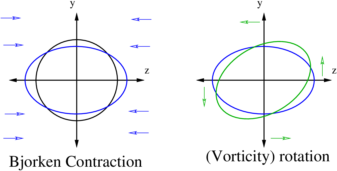
The relation between $\tau_{\Pi}$ and $\lambda_{2}$ , and the sign of $\lambda_{2}$ , also have fairly simple interpretations. First the sign. Physically $\lambda_{2}$ tells what happens to a system which is both Bjorken contracting (nonzero $\sigma_{zz}$ ) and rotating (nonzero vorticity, say $\Omega_{zy}>0$ ). As illustrated in Figure 3, in this case the contraction makes the particle distribution become prolate; but the vorticity skews this distribution so it is not aligned with the Bjorken contraction axis. That should lead to a positive $T_{yz}$ , which for $\sigma_{zz}<0$ and $\Omega_{zy}>0$ requires $\lambda_{2}<0$ . The proportionality constant depends on how large the original $zz$ asymmetry was, which depends on $\eta$ , and on how long the induced $xy$ skewed distribution “lives,” which is set by $\tau_{\Pi}$ . Accounting for numerical factors turns out to give $\lambda_{2}=-2\eta\tau_{\Pi}$ , as we find.

Next consider $\lambda_{1}$ . For our example of Bjorken contraction,

\Pi_{zz}=-\eta\sigma_{zz}+\lambda_{1}(\sigma_{zl}\sigma_{zl}-\delta_{zz}\sigma_{lm}^{2}/3)=\eta(2c)+\lambda_{1}(2c^{2})\,.

Therefore a positive $\lambda_{1}$ means that for Bjorken contraction, the stress tensor deviates further than normal from equilibrium. On the other hand, reversing the sign of $c$ to consider Bjorken expansion, the deviation from the equilibrium value of $\Pi_{zz}$ is reduced. Therefore $\lambda_{1}$ tells whether equilibration is accelerated for Bjorken expansion ( $\lambda_{1}$ positive) or Bjorken contraction ( $\lambda_{1}$ negative).¹⁵¹⁵ 15 $\lambda_{1}$ does NOT indicate the “anomalous viscosity” expected from plasma instabilities [35]. “Anomalous viscosity,” for which $|\Pi_{ij}|$ falls below the linear term for all flow patterns, would be indicated by a large positive value for the third order term $\Pi_{ij}\propto\sigma_{ij}\sigma_{lm}\sigma_{lm}$ .

Our calculation shows that there are 3 contributions to $\lambda_{1}$ . First, if the particle distribution has already become prolate, then further Bjorken contraction generates a different amount of prolateness than it would from a spherically symmetric distribution. This is the part contributed by $2P^{\mu}\partial_{\mu}f_{1}$ . The sign turns out to be positive and the magnitude dominates all contributions to $\lambda_{1}$ .

The contribution to $\lambda_{1}$ from ${\cal C}_{11}$ reflects the change, in going from a thermal to a prolate momentum distribution, in the set of scattering targets a particle has. Whether this accelerates equilibration or slows it down depends on typical scattering angles in a rather complicated way, indicated by the rather complicated angular integrations involved in Eq. (60) and Eq. (52). This leads to considerable angular cancellation. For instance, in $\lambda\phi^{4}$ theory, where the matrix element ${\cal M}^{2}=\lambda^{2}$ shows no preference for particular scattering angles, the contribution to $\lambda_{1}$ from ${\cal C}_{11}$ is $+0.0372$ . If we replace Bose with Boltzmann statistics in $\lambda\phi^{4}$ theory, the cancellation on angular averages becomes exact and ${\cal C}_{11}$ gives no contribution to $\lambda_{1}$ . In QCD the contribution is also small, due to significant angular cancellation; for 3-flavor QCD the ${\cal C}_{11}$ contribution to $\lambda_{1}$ varies between $-0.18$ at weak to $-0.45$ at stronger coupling. The negative sign means that prolate distributions show accelerated equilibration.

The contribution to $\lambda_{1}$ from ${\cal C}_{1;{\cal M}_{1}}$ reflects changes in the efficiency of scattering and collinear splitting because of changes in plasma screening. This is interesting because it is where the precursors of plasma instabilities (see [36, 37, 38]) can enter the game. An anisotropic particle distribution weakens the stabilizing effect of plasma screening for certain particle directions $\hat{p}$ and exchange momenta ${\bf q}$ . In particular, in directions where $f_{1}({\bf p})$ is positive, these particles have enhanced scattering via soft magnetic ( $G_{T}$ ) gluon exchange with ${\bf q}\perp{\bf p}$ . One might guess that this leads to a large negative contribution to $\lambda_{1}$ . However we find that extensive angular cancellations occur which make the contribution arising from elastic scatterings very small, and free of IR divergences, see the discussion at the end of Appendix A.3.

The same does not happen for collinear splitting. If the particle distribution becomes prolate, the approach to equilibration would be accelerated ( $\lambda_{1}<0$ ) if the particles traveling in the prolate ( $z$ ) direction show a higher rate of collinear splitting, since such splitting is an equilibrating process. The rate of collinear splitting depends on the efficiency of transverse momentum diffusion. But the proto-plasma instability caused by a prolate distribution is automatically the right one to enhance such transverse momentum diffusion for particles moving along the $z$ axis.¹⁶¹⁶ 16 It also slows down transverse momentum diffusion for particles in the “equator” of the prolate distribution, slowing their approach to equilibrium. The angle averaged rate of splitting remains constant at this order. But $\lambda_{1}$ does not depend on this angle averaged rate; it is dominated by what happens along the axis of prolateness (or oblateness). Therefore we can get the right sign by paying attention only to what happens to particles along the $z$ axis. Therefore the contribution of collinear splitting processes in ${\cal C}_{1;{\cal M}_{1}}$ should contribute negatively to $\lambda_{1}$ and give the first hints of the effects of plasma instabilities.

The fractional change in scattering efficiency due to $f_{1}$ grows at small momentum exchange as $1/q^{2}$ . This behavior is expected; for weakly anisotropic plasmas only the smallest $q$ ’s show plasma instabilities, which appear in perturbation theory to give an infinite scattering rate. Since $\sigma_{ij}$ is treated as formally infinitesimal, there is no finite momentum $q$ which becomes unstable, but the restoring effect of the plasma is changed more and more for softer and softer magnetic $q$ . This leads to an IR log divergence in the total momentum transfer rate $\int d^{2}q_{\perp}q_{\perp}^{2}C(q_{\perp})$ , see Appendix A.5. Therefore the change to the rate of collinear splitting is log divergent when computed at leading perturbative order.

This means that our result for $\lambda_{1}$ actually includes a (negative in sign) logarithmically divergent contribution, at least using the perturbative calculational tools we employ here. The log is $\ln(m_{\rm D}/\epsilon)$ , with $\epsilon$ an artificially imposed minimum momentum transfer, implemented by modifying $q^{2}\rightarrow q^{2}+\epsilon$ in the denominator for transverse gauge boson exchange when computing this process.

Physically, there really will be a limit on the infrared end of momentum transfer. In QCD we expect $\epsilon\sim g^{2}T$ the magnetic screening scale. This is where the perturbative treatment of plasma corrections to gauge field propagation breaks down. Unfortunately we cannot compute the exact form of this cutoff (the constant under the log, $\ln(m_{\rm D}/g^{2}T)+k$ ) because this momentum region is strongly coupled. Similarly, we expect that in QED the perturbative treatment of screening also breaks down for $q\sim e^{4}T$ , where the physical distance of particle propagation involved is of order the large-angle scattering length and the electron propagators cease to behave like Eikonal propagators (as assumed in the hard-loop computation of self-energies). It might be possible to compute the constant under the log, $\ln(m_{\rm D}/e^{4}T)+k$ , but we have not done so.

As a result, we have not actually been able to compute the complete finite-coupling value of $\lambda_{1}$ . Rather, we have guessed what the cutoff $\epsilon$ on transverse momentum should be; we set $\epsilon=g^{2}T/2$ in QCD and $\epsilon=e^{4}T/10$ in QED. This leaves an uncertainty in our results, set by the coefficient on the $\ln(m_{\rm D}/\epsilon)$ term arising from $C_{1;{\cal M}_{1}}$ from collinear splitting processes. Fortunately, it turns out that this contribution is numerically tiny. If the constant under the log shifts by 1 (the correct cutoff is $g^{2}T/5.4$ rather than $g^{2}T/2$ ) then our result for $\lambda_{1}$ changes by less than $0.003$ in 3-flavor QCD and less than $0.0003$ in pure-glue QCD or QED.

The extreme smallness of this effect arises as the product of several small things. First, collinear splittings are not that important in driving thermalization. Second, the splitting rate is reduced in some directions, and there is some angular averaging which reduces the total importance of the shift in the splitting rate. Third, the change to the splitting rate in any specific direction also turns out to be numerically small. This is another indication that in practice the physical importance of plasma instabilities turns out not to be very large.

We end the discussion by commenting about the range of validity of our calculation. In Figures 1, 2 we have plotted our results out to $m_{\rm D}/T=3$ , which corresponds to quite a large coupling $\alpha_{\rm s}=.48$ in 3-flavor and $\alpha_{\rm s}=.72$ in pure-glue QCD. The calculation certainly cannot be believed at such couplings; probably it becomes inadequate beyond $m_{\rm D}/T=1$ (see [16] for a next-to-leading order calculation of a similar transport coefficient). The scaled results for $\tau_{\Pi}$ and $\lambda_{1}$ are weakly dependent on details of the theory, as shown by the almost identical results for $\lambda\phi^{4}$ theory and QCD at weak and relatively strong coupling. But they rely in an essential way on the validity of kinetic theory. There will be ${\cal O}(\alpha_{\rm s})$ corrections which cannot be incorporated in kinetic theory, which we generically expect to change the shape of the curves and which we do not know how to compute. Therefore the flatness of the curves in the figures can only be taken seriously at small $m_{\rm D}/T$ (we would guess below $m_{\rm D}/T=1.5$ ).

Acknowledgements

We would like to thank Makoto Natsuume for suggesting we pursue this calculation. GM would like to thank the department of theoretical physics at Bielefeld University for hospitality while this work was completed, and the Alexander von Humboldt Foundation for its support through a F. W. Bessel prize. This work was supported in part by the Natural Sciences and Engineering Research Council of Canada.

Appendix A Matrix elements at nonzero $\sigma_{\mu\nu}$

A particle of momentum $P$ scattering from a particle of momentum $K$ via gauge boson exchange with a soft exchange momentum $Q$ , $|Q^{2}|\ll|P\cdot K|$ does so with a leading order matrix element (suppressing group factors)

{\cal M}=2P^{\mu}G_{\mu\nu}2K^{\mu}\,,\qquad G^{-1}_{\mu\nu}=Q^{2}g_{\mu\nu}-Q_{\mu}Q_{\nu}-\Pi_{\mu\nu}[f]+\mbox{(Gauge fix)}\,,

(84)

with $G,\Pi$ understood as the retarded propagator and self-energy. What is relevant here is that $\Pi_{\mu\nu}$ explicitly depends on the medium through its distribution function $f$ . Write it as $\Pi_{\mu\nu}[f]=\Pi_{\mu\nu,\rm eq}+\delta\Pi_{\mu\nu}[f_{1}]$ plus terms of higher order. Then the squared matrix element becomes

$\displaystyle\|{\cal M}\|^{2}$	$\displaystyle=$	$\displaystyle{\cal M}_{0}{\cal M}_{0}^{}+{\cal M}_{0}{\cal M}_{1}^{}+{\cal M}_{0}^{*}{\cal M}_{1}+{\cal O}(\lambda^{2})\,,$
$\displaystyle{\cal M}_{0}$	$\displaystyle=$	$\displaystyle 2P^{\mu}G_{\mu\nu}2K^{\nu}\,,$
$\displaystyle{\cal M}_{1}$	$\displaystyle=$	$\displaystyle 2P^{\mu}G_{\mu\alpha}\,\delta\Pi^{\alpha\beta}[f_{1}]\,G_{\beta\nu}2K^{\nu}\,,$	(85)

where to simplify notation $G$ now means the equilibrium propagator. Since $\Pi$ is suppressed relative to $G^{-1}$ unless $Q^{2}\sim g^{2}T^{2}$ , we can freely treat $Q^{2}$ as small in what follows, systematically expanding whenever possible in $p,k\gg q,q^{0}$ . Similar expressions are also needed for fermionic exchange processes and the fermionic self-energy.

Our goal in this appendix is to evaluate Eq. (62). Clearly as a first step we need to evaluate $\delta\Pi^{\alpha\beta}$ and its fermionic equivalent; then we need to use this to evaluate $({\cal M}_{0}{\cal M}_{1}^{*}+{\rm h.c.})$ and perform the momentum integrations. In addition, the collinear splitting rate is sensitive to $\delta\Pi$ because it depends on the rate of soft momentum exchange; so we will have to revisit the rate of collinear splittings as well.

A.1 Bosonic self-energy

With the sign convention established in Eq. (84), for soft 4-momentum $Q=(q^{0},{\bf q})$ the leading order (retarded, hard-loop) self-energy is [39]

\Pi^{\mu\nu}(Q)=\sum_{R}g^{2}T_{R}\int\frac{d^{3}{\bf p}}{(2\pi)^{3}}\frac{\partial f(p)}{\partial p^{k}}\left[v^{\mu}g^{k\nu}-\frac{v^{\mu}v^{\nu}q^{k}}{{\bf v}\cdot{\bf q}-q^{0}-i\epsilon}\right]

(86)

where ${\bf v}={\bf p}/p$ and $p=|{\bf p}|$ as usual. The sum is over species, spin and particle/antiparticle but not color. Setting $f=f_{0}$ and using

\sum_{R}g^{2}T_{R}\int\frac{d^{3}p}{(2\pi)^{3}}(-df_{0}/dp)=m_{\rm D}^{2}=2m_{g}^{2}

(87)

recovers the usual HTL self-energies: in strict Coulomb gauge, which we use henceforth,

	$\displaystyle G_{00}=\frac{1}{-q^{2}-\Pi_{00}(Q)}\equiv\frac{q^{2}-\omega^{2}}{q^{2}}G_{L}\,,$		$\displaystyle\Pi_{00}(Q)=m_{g}^{2}\left(2-\frac{\omega}{q}\ln\frac{\omega{+}q}{\omega{-}q}\>\right)\,,$		(88)
	$\displaystyle G_{ij}=\frac{\delta_{ij}-\hat{q}_{i}\hat{q}_{j}}{q^{2}-\omega^{2}-\Pi_{T}(Q)}\equiv(\delta_{ij}-\hat{q}_{i}\hat{q}_{j})G_{T}\,,$		$\displaystyle\Pi_{T}(Q)=-m_{g}^{2}\left(\frac{\omega^{2}}{q^{2}}+\frac{\omega(q^{2}-\omega^{2})}{2q^{3}}\ln\frac{\omega{+}q}{\omega{-}q}\>\right)\,.$

(Throughout the log has a $\mp i\pi$ , with $-$ in retarded propagators $G,\Pi$ and $+$ in advanced propagators $G^{*},\Pi^{*}$ .) Now we want to compute $\delta\Pi(Q)$ using

f_{1}(p)=\frac{\beta\sigma_{ij}}{2}{v_{\langle i}v_{j\rangle}}\chi(p)

(89)

where $\chi(p)=\beta^{2}p^{2}{\tilde{\chi}}(p)$ . Then

\frac{\partial f_{1}}{\partial p^{k}}=\frac{\beta\sigma_{ij}}{2}\left(\frac{v_{i}\delta_{jk}+v_{j}\delta_{ik}-2v_{i}v_{j}v_{k}}{p}\chi(p)+{v_{\langle i}v_{j\rangle}}v_{k}\chi^{\prime}(p)\right)\,.

(90)

The integration separates into an angular and a radial part. Integrating the $\chi^{\prime}$ radial term by parts gives

	$\displaystyle\delta\Pi_{\mu\nu}(Q)$	$\displaystyle=$	$\displaystyle\beta\left(\sum_{R}\frac{g^{2}T_{R}}{2\pi^{2}}\int pdp\chi(p)\right)\times A_{\mu\nu}\equiv\beta\delta m_{g}^{2}A_{\mu\nu}\,,$
	$\displaystyle A_{\mu\nu}$	$\displaystyle=$	$\displaystyle\frac{\sigma_{ij}}{2}\int d\Omega_{\bf v}\left(v_{i}\delta_{jk}+v_{j}\delta_{ik}-4v_{i}v_{j}v_{k}+\frac{2}{3}\delta_{ij}v_{k}\right)\left(v^{\mu}g^{k\nu}-\frac{v^{\mu}v^{\nu}q^{k}}{v_{l}q_{l}-q^{0}}\right)\,.$		(91)

This depends on $Q$ only through $\hat{{\bf q}}$ and $q^{0}/q$ ; henceforth we rescale ${\bf q}$ to be a unit vector, and $q^{0}=\eta\equiv q^{0}/|{\bf q}|$ .

First let us find $A_{00}$ :

A_{00}=-\frac{\sigma_{ij}}{2}\int d\Omega_{\bf v}\frac{v_{i}q_{j}+v_{j}q_{i}-4v_{i}v_{j}{\bf v}\cdot{\bf q}+2\delta_{ij}{\bf v}\cdot{\bf q}/3}{{\bf v}\cdot{\bf q}-q^{0}}\equiv\frac{\sigma_{ij}}{2}{q_{\langle i}q_{j\rangle}}A

(92)

(since this is the only possible tensorial structure). To find $A$ , contract the integral with $q_{i}q_{j}$ and define $x={\bf q}\cdot{\bf v}$ :

A=\frac{3}{4}\int_{-1}^{1}dx\frac{4x^{3}-8x/3}{x-\eta}=2(3\eta^{2}-1)-(3\eta^{3}-2\eta)\ln\frac{\omega{+}q}{\omega{-}q}\>\,.

(93)

Next consider $A^{0k}$ : in practice we will only need

	$\displaystyle(\delta_{kl}-q_{k}q_{l})A^{0l}$	$\displaystyle=$	$\displaystyle\frac{\sigma_{ij}}{2}\int d\Omega_{\bf v}\frac{(-v_{k}+q_{k}q\cdot v)(v_{i}q_{j}+v_{j}q_{i}-4v_{i}v_{j}{\bf v}\cdot{\bf q}+2\delta_{ij}{\bf v}\cdot{\bf q}/3)}{{\bf v}\cdot{\bf q}-q^{0}}$		(94)
		$\displaystyle=$	$\displaystyle(\sigma_{ij}/2)B\left[q_{i}\delta_{jk}+q_{j}\delta_{ik}-2q_{i}q_{j}q_{k}\right]\,.$		(94)

The coefficient is found by contracting with $q_{i}\delta_{jk}$ :

B=\frac{11\eta-12\eta^{3}}{6}+\frac{(1-\eta^{2})(1-4\eta^{2})}{4}\ln\frac{\omega{+}q}{\omega{-}q}\>\,.

(95)

Finally we need $A_{lm}$ . In practice we need it only contracted against transverse projectors:

A_{lm}=\frac{\sigma_{ij}}{2}\int d\Omega_{\bf v}\left(v_{i}\delta_{jk}+v_{j}\delta_{ik}-4v_{i}v_{j}v_{k}+\frac{2}{3}\delta_{ij}v_{k}\right)\left(v_{l}g_{mk}-\frac{v_{l}v_{m}q_{k}}{{\bf v}\cdot{\bf q}-q^{0}}\right)

(96)

must be of form (defining $\hat{\delta}_{lm}\equiv\delta_{lm}-q_{l}q_{m}$ )

\hat{\delta}_{lr}A_{rs}\hat{\delta}_{ms}=\frac{\sigma_{ij}}{2}\left(\!C_{1}\hat{\delta}_{lm}\;{q_{\langle i}q_{j\rangle}}+C_{2}\left[\hat{\delta}_{il}\hat{\delta}_{jm}+(i\leftrightarrow j)-\frac{2\delta_{ij}}{3}\hat{\delta}_{lm}\right]\right).

(97)

Contracting both the quantity in parenthesis and the original integral expression with two independent tensors, such as $q_{i}q_{j}\delta_{lm}$ and $\delta_{il}\delta_{jm}$ , determines the coefficients:

	$\displaystyle C_{1}$	$\displaystyle=$	$\displaystyle\frac{(1-\eta^{2})(15\eta^{2}-4)}{6}+\frac{\eta(1-\eta^{2})(3-5\eta^{2})}{4}\ln\frac{\omega{+}q}{\omega{-}q}\>\,,$
	$\displaystyle C_{2}$	$\displaystyle=$	$\displaystyle\frac{(1-\eta^{2})(2-3\eta^{2})}{6}-\frac{\eta(1-\eta^{2})^{2}}{4}\ln\frac{\omega{+}q}{\omega{-}q}\>\,.$		(98)

A.2 Fermionic self-energy

The fermionic self-energy correction is [39] (convention $1/(\hbox to0.0pt{\hbox to7.90555pt{\hfil/\hfil}\hss}Q-\Sigma)$ )

\Sigma(Q)=-\frac{g^{2}C_{\rm f}}{2\pi^{2}}\int\frac{p^{2}dp}{2p}\int d\Omega_{{\bf p}}\left[2f_{g}+f_{q}+f_{\bar{q}}\right]\frac{\hat{\bf p}\cdot\gamma-\gamma^{0}}{\hat{\bf p}\cdot{\bf q}-q^{0}}

(99)

Hence the equilibrium value is

\Sigma_{\rm eq}(Q)=\frac{g^{2}C_{\rm f}T^{2}}{16q}\left(\gamma_{i}\hat{q}_{i}\left[-2+\eta\ln\frac{\omega{+}q}{\omega{-}q}\>\right]-\gamma^{0}\ln\frac{\omega{+}q}{\omega{-}q}\>\right)\,.

(100)

Taking $f_{1}$ from Eq. (89), the correction term is

	$\displaystyle\delta\Sigma$	$\displaystyle=$	$\displaystyle\beta\left(\frac{g^{2}C_{\rm f}}{2\pi^{2}q}\int pdp(\chi_{g}(p)+\chi_{q}(p))\right)\frac{\sigma_{ij}}{2}\int d\Omega_{\bf v}\left(v_{i}v_{j}-\frac{\delta_{ij}}{3}\right)\frac{-v_{k}\gamma_{k}+\gamma^{0}}{{\bf v}\cdot\hat{q}-\eta}$		(101)
		$\displaystyle\equiv$	$\displaystyle\beta\left(\frac{g^{2}C_{\rm f}}{2\pi^{2}q}\int pdp(\chi_{g}(p)+\chi_{q}(p))\right)A\equiv\beta\frac{\delta m_{f}^{2}}{2q}A\,.$		(101)

We have $A=A_{0}\gamma^{0}+A_{k}\gamma_{k}$ .

Start with $A^{0}$ :

$\displaystyle A^{0}$	$\displaystyle=$	$\displaystyle-\frac{\sigma_{ij}}{2}\int d\Omega_{\bf v}\frac{v_{i}v_{j}-\delta_{ij}/3}{{\bf v}\cdot\hat{\bf q}-\eta}$	(102)
	$\displaystyle=$	$\displaystyle-\frac{\sigma_{ij}}{2}\;{q_{\langle i}q_{j\rangle}}\left(\frac{3}{4}\int_{-1}^{1}dx\frac{x^{2}-1/3}{x-\eta}\right)$
	$\displaystyle=$	$\displaystyle\frac{\sigma_{ij}}{2}\;{q_{\langle i}q_{j\rangle}}\left(\frac{-3\eta}{2}+\frac{3\eta^{2}-1}{4}\ln\frac{\omega{+}q}{\omega{-}q}\>\right)\,.$

Similarly

	$\displaystyle A_{k}$	$\displaystyle=$	$\displaystyle-\frac{\sigma_{ij}}{2}\int d\Omega_{\bf v}v_{k}\frac{v_{i}v_{j}-\delta_{ij}/3}{{\bf v}\cdot\hat{\bf q}-\eta}$		(103)
		$\displaystyle=$	$\displaystyle\frac{\sigma_{ij}}{2}\left(\kappa_{1}q_{k}\;{q_{\langle i}q_{j\rangle}}+\kappa_{2}\left[q_{i}\delta_{jk}+q_{j}\delta_{ik}-\frac{2}{3}\delta_{ij}q_{k}\right]\right)\,.$		(103)

Determine the coefficients by contracting with $q_{i}q_{j}q_{k}$ and with $q_{i}\delta_{jk}$ :

\frac{2\kappa_{1}+4\kappa_{2}}{3}=\frac{1}{6}\int_{-1}^{1}dx\frac{x-3x^{3}}{x-\eta}\,,\qquad\frac{2\kappa_{1}+10\kappa_{2}}{3}=\frac{1}{3}\int_{-1}^{1}dx\frac{-x}{x-\eta}\,.

(104)

Therefore

	$\displaystyle\kappa_{1}$	$\displaystyle=$	$\displaystyle\frac{4-15\eta^{2}}{6}+\frac{-3\eta+5\eta^{3}}{4}\ln\frac{\omega{+}q}{\omega{-}q}\>\,,$
	$\displaystyle\kappa_{2}$	$\displaystyle=$	$\displaystyle\frac{-2+3\eta^{2}}{6}+\frac{\eta-\eta^{3}}{4}\ln\frac{\omega{+}q}{\omega{-}q}\>\,.$		(105)

Replacing $\gamma^{\mu}\rightarrow Q^{\mu}$ in Eq. (99) gives an angular averaged integral and so $Q_{\mu}\delta\Sigma^{\mu}=0$ , or $\eta A^{0}-(\kappa_{1}+2\kappa_{2})=0$ , which is satisfied. This is a fast way to see that the correction to the hard propagation velocity $m_{\infty}^{2}$ is isotropic.

A.3 Bosonic $2\leftrightarrow 2$ contribution to $C_{1;{\cal M}_{1}}$

We work in the plasma rest frame and systematically approximate that the incoming particle energies $p,k$ are much larger than the transfer momentum $q$ or frequency $|q^{0}|\leq q$ . Using the integration variable parametrization of [19], the contribution to $\Pi_{ij,\rm 2\;order}$ is

	$\displaystyle\Pi_{ij,{\rm 2\;order}}$	$\displaystyle\supset$	$\displaystyle\frac{A_{ab}}{2^{8}\pi^{5}}\int_{0}dp\int_{0}dk\int_{0}qdq\int_{-1}^{1}d\eta\int_{0}^{2\pi}\frac{d\phi}{2\pi}\>f_{0}(p)[1{\pm}f_{0}(p)]f_{0}(k)[1{\pm}f_{0}(k)]$		(106)
			$\displaystyle\times T{\bar{\chi}}_{ij}(p)\frac{\sigma_{rs}}{2}\left({\bar{\chi}}_{rs}({\bf p})+{\bar{\chi}}_{rs}({\bf k})-{\bar{\chi}}_{rs}({\bf p}^{\prime})-{\bar{\chi}}_{rs}({\bf k}^{\prime})\vphantom{\Big\|}\right)\Big({\cal M}_{0}^{}{\cal M}_{1}+{\cal M}_{0}{\cal M}_{1}^{}\Big).\qquad\;$		(106)

Here ${\cal M}_{0},{\cal M}_{1}$ are to be normalized as in Eq. (85); we have absorbed all color factors into $A_{ab}$ which in SU( $N_{\rm c}$ ) gauge theory with $n_{\rm f}$ fermions is $16d_{\rm f}^{2}n_{\rm f}^{2}C_{\rm f}^{2}/d_{\rm A}$ for fermion-fermion scattering, $16d_{\rm f}n_{\rm f}C_{\rm f}C_{\rm A}$ for fermion-boson scattering and $4d_{\rm A}C_{\rm A}^{2}$ for boson-boson scattering. Symmetry between $p,p^{\prime},k,k^{\prime}$ allows us to replace

{\bar{\chi}}_{ij}(p)\rightarrow\frac{1}{4}\Big({\bar{\chi}}_{ij}({\bf p})+{\bar{\chi}}_{ij}({\bf k})-{\bar{\chi}}_{ij}({\bf p}^{\prime})-{\bar{\chi}}_{ij}({\bf k}^{\prime})\Big)

(107)

and small $q$ approximations allow [19]

\Big({\bar{\chi}}_{ij}({\bf p})+{\bar{\chi}}_{ij}({\bf k})-{\bar{\chi}}_{ij}({\bf p}^{\prime})-{\bar{\chi}}_{ij}({\bf k}^{\prime})\Big)\simeq-q\beta^{3}\Big(2\hat{{\bf p}}_{\langle i}\hat{{\bf q}}_{j\rangle}p{\bar{\chi}}(p)+\eta\hat{{\bf p}}_{\langle i}\hat{{\bf p}}_{j\rangle}p^{2}{\bar{\chi}}^{\prime}(p)-(p\rightarrow k)\Big)

(108)

and similarly for the ${\bar{\chi}}_{lm}$ term.

All angles are determined by the $\eta,\phi$ variables; in particular $x_{pq}=\eta=x_{kq}$ and $x_{pk}=\eta^{2}+(1{-}\eta^{2})\cos\phi$ . Therefore, extracting a factor of $pk$ from ${\cal M}_{0}$ and ${\cal M}_{1}$ , $\tilde{\cal M}_{0}\equiv{\cal M}_{0}/pk$ , the integrals over the magnitudes $p,k$ factorize from the integrals over $q,\omega,\phi$ . Defining the integrals

\left.\begin{array}[]{c}K_{0}\\ K_{1}\\ K_{2}\\ K_{3}\\ K_{4}\\ K_{5}\\ \end{array}\right\}=\int_{0}^{\infty}dpp^{2}(-f_{0}^{\prime}(p))\times\left\{\begin{array}[]{l}1\\ 4p^{2}{\bar{\chi}}^{2}\\ 4p^{3}{\bar{\chi}}{\bar{\chi}}^{\prime}\\ p^{4}({\bar{\chi}}^{\prime})^{2}\\ 2p{\bar{\chi}}\\ p^{2}{\bar{\chi}}^{\prime}\\ \end{array}\right.

(109)

we need, for the double fermion term for instance,

$\displaystyle\frac{\beta^{5}A_{ff}}{2^{10}\pi^{5}}$	$\displaystyle\int_{0}q^{3}dq\int_{-1}^{1}d\eta\int\frac{d\phi}{2\pi}\Big(\tilde{\cal M}_{0}\tilde{\cal M}_{1}^{}+\tilde{\cal M}_{0}^{}\tilde{\cal M}_{1}\Big)\frac{\sigma_{lm}}{2}$	(110)
	$\displaystyle\times\Big(2K_{0}K_{1}{\hat{\bf p}_{\langle i}\hat{\bf q}_{j\rangle}}{\hat{\bf p}_{\langle l}\hat{\bf q}_{m\rangle}}+2K_{0}K_{2}\eta{\hat{\bf p}_{\langle i}\hat{\bf q}_{j\rangle}}{\hat{\bf p}_{\langle l}\hat{\bf p}_{m\rangle}}+2K_{0}K_{3}\eta^{2}{\hat{\bf p}_{\langle i}\hat{\bf p}_{j\rangle}}{\hat{\bf p}_{\langle l}\hat{\bf p}_{m\rangle}}$
	$\displaystyle\qquad\;-2K_{4}^{2}{\hat{\bf p}_{\langle i}\hat{\bf q}_{j\rangle}}{\hat{\bf k}_{\langle l}\hat{\bf q}_{m\rangle}}-4K_{4}K_{5}\eta{\hat{\bf p}_{\langle i}\hat{\bf p}_{j\rangle}}{\hat{\bf k}_{\langle l}\hat{\bf q}_{m\rangle}}-2K_{5}^{2}\eta^{2}{\hat{\bf p}_{\langle i}\hat{\bf p}_{j\rangle}}{\hat{\bf k}_{\langle l}\hat{\bf k}_{m\rangle}}\Big)\,,$

where we used $p\leftrightarrow k$ symmetry to simplify some terms. The matrix element squared is

$\displaystyle\tilde{\cal M}^{*}_{0}\tilde{\cal M}_{1}$	$\displaystyle=$	$\displaystyle 16\left(G_{00}^{}+(1{-}\eta^{2})\cos\phi G_{T}^{}\right)\times\beta\delta m_{g}^{2}\frac{\sigma_{rs}}{2}$	(111)
		$\displaystyle\times\bigg(G_{00}^{2}A{\hat{q}_{\langle r}\hat{q}_{s\rangle}}+G_{00}G_{T}B\left[{\hat{{\bf p}}_{\langle r}\hat{{\bf q}}_{s\rangle}}+{\hat{{\bf k}}_{\langle r}\hat{{\bf q}}_{s\rangle}}-2\eta{\hat{{\bf q}}_{\langle r}\hat{{\bf q}}_{s\rangle}}\right]$
		$\displaystyle\quad\;+G_{T}^{2}\left[C_{1}(1{-}\eta^{2})\cos\phi{\hat{{\bf q}}_{\langle r}\hat{{\bf q}}_{s\rangle}}+2C_{2}({\hat{{\bf p}}_{\langle r}\hat{{\bf k}}_{s\rangle}}-\eta{\hat{{\bf k}}_{\langle r}\hat{{\bf q}}_{s\rangle}}-\eta{\hat{{\bf p}}_{\langle r}\hat{{\bf q}}_{s\rangle}}+\eta^{2}{\hat{{\bf q}}_{\langle r}\hat{{\bf q}}_{s\rangle}})\right]\bigg).$

The integral $\int_{0}^{2\pi}\frac{d\phi}{2\pi}$ can always be done analytically by replacing $\cos^{(0,1,2,3,4)}\phi=(1,0,\frac{1}{2},0,\frac{3}{8})$ . Using repeatedly Eq. (59) the evaluation of Eq. (110) is now straightforward, if lengthy.

One potential pitfall in performing the $q,\eta$ integrals in Eq. (110) is the possibility of an infrared small $q$ divergence. This can come about because $G_{T}(q,\eta)$ behaves, for $q<m_{\rm D}$ and $\eta<q^{2}/m_{\rm D}^{2}$ , like $G_{T}\sim 1/q^{2}$ . The integration region over which this behavior applies is $q^{5}dq$ but the $G_{T}^{*}G_{T}^{2}$ term in Eq. (111) is $1/q^{6}$ so there is a potential log divergence. To determine whether this divergence occurs it is sufficient to approximate $\eta=0$ in the integrands, other than in $G_{T}$ . In this limit $C_{1}=-2C_{2}$ . Only the $K_{0}K_{1}$ and $K_{4}^{2}$ terms are zero-order in $\eta$ so only they need be computed; the relevant global angular averages are

	$\displaystyle K_{0}K_{1}(\ldots)\cos\phi\int d\Omega_{\rm global}{\hat{\bf p}_{\langle i}\hat{\bf q}_{j\rangle}}{\hat{\bf p}_{\langle l}\hat{\bf q}_{m\rangle}}\Big({\hat{{\bf p}}_{\langle r}\hat{{\bf k}}_{s\rangle}}-\cos\phi{\hat{{\bf q}}_{\langle r}\hat{{\bf q}}_{s\rangle}}\Big)\,,$
	$\displaystyle K_{4}^{2}(\ldots)\cos\phi\int d\Omega_{\rm global}{\hat{\bf p}_{\langle i}\hat{\bf q}_{j\rangle}}{\hat{\bf k}_{\langle l}\hat{\bf q}_{m\rangle}}\Big({\hat{{\bf p}}_{\langle r}\hat{{\bf k}}_{s\rangle}}-\cos\phi{\hat{{\bf q}}_{\langle r}\hat{{\bf q}}_{s\rangle}}\Big)\,.$		(112)

Applying Eq. (59) setting $x_{pq}=0=x_{kq}$ and $x_{pk}=\cos\phi$ and averaging over $\phi$ , one finds that each term happens to vanish, so the potential IR divergence does not occur.

A.4 Fermionic $2\leftrightarrow 2$ contribution to $C_{1;{\cal M}_{1}}$

The infrared region of virtual fermion exchange is also important at leading order for transport [19]. The contribution is still described by Eq. (106) but with $A=32n_{\rm f}C_{\rm f}^{2}d_{\rm f}$ each for pair annihilation and Compton scattering. Since the matrix element is less infrared singular, we can approximate ${\bar{\chi}}_{rs}({\bf p})={\bar{\chi}}_{rs}({\bf p}^{\prime})$ and similarly for $k$ . But if ${\bar{\chi}}(p)$ represents a fermion, then ${\bar{\chi}}(k),{\bar{\chi}}(k^{\prime})$ represent a quark and gluon for annihilation, but a gluon and quark for Compton scattering. Therefore, summing over the processes, the $p,k$ cross-terms cancel and we may approximate

\bar{\chi}_{ij}(p)\left({\bar{\chi}}_{rs}({\bf p})+{\bar{\chi}}_{rs}({\bf k})-{\bar{\chi}}_{rs}({\bf p}^{\prime})-{\bar{\chi}}_{rs}({\bf k}^{\prime})\vphantom{\Big|}\right)=\frac{1}{2}\Big(\bar{\chi}_{ij,q}(p)-\bar{\chi}_{ij,g}(p)\Big)\Big(\bar{\chi}_{lm,q}(p)-\bar{\chi}_{lm,g}(p)\Big)

(113)

where the subscripts $q,g$ indicate if the species is a quark or a gluon. This simplifies matters considerably; pulling a factor $pk$ out of ${\cal M}^{2}$ , the $p,k$ integrals we need are

\beta^{5}\int dpp^{5}f_{0,f}(p)[1{+}f_{0,b}(p)]({\bar{\chi}}_{q}-{\bar{\chi}}_{g})^{2}\;\int dkkf_{0,f}(k)[1{+}f_{0,b}(k)]

(114)

which multiply the $q,\eta$ integral

\int qdq\int_{-1}^{1}d\eta\int\frac{d\phi}{2\pi}\frac{\sigma_{lm}}{2}\hat{p}_{\langle i}\hat{p}_{j\rangle}\hat{p}_{\langle l}\hat{p}_{m\rangle}\Big(\tilde{{\cal M}}_{0}^{*}\tilde{{\cal M}}_{1}+{\rm h.c.}\Big)

(115)

with

\displaystyle\tilde{\cal M}_{0}^{*}\tilde{\cal M}_{1}

\displaystyle=

\displaystyle\frac{1}{(\tilde{Q}^{2})^{2}(\tilde{Q}^{*})^{2}}\>{\rm Tr}\>\hat{\hbox to0.0pt{\hbox to5.03125pt{\hfil/\hfil}\hss}p}\hbox to0.0pt{\hbox to5.55557pt{\hfil/\hfil}\hss}\tilde{Q}\delta\hbox to0.0pt{\hbox to7.22223pt{\hfil/\hfil}\hss}\Sigma\hbox to0.0pt{\hbox to5.55557pt{\hfil/\hfil}\hss}\tilde{Q}\hat{\hbox to0.0pt{\hbox to5.52084pt{\hfil/\hfil}\hss}k}\hbox to0.0pt{\hbox to5.55557pt{\hfil/\hfil}\hss}\tilde{Q}^{*}

(116)

with $\tilde{Q}^{\mu}\equiv Q^{\mu}-\Sigma^{\mu}_{\rm eq}$ and $\delta\Sigma^{\mu}$ as given in Appendix A.2. The trace and global angular average are straightforward but tedious.

A.5 Collinear $1\leftrightarrow 2$ contribution to $C_{1;{\cal M}_{1}}$

According to [20], the rate at which a particle in the thermal medium splits into two is given by

	$\displaystyle{\cal C}_{1\leftrightarrow 2}[f(p)]$	$\displaystyle=$	$\displaystyle\frac{(2\pi)^{3}}{2p^{2}}\sum_{bc}\int_{0}^{\infty}dp^{\prime}dk^{\prime}\delta(p-p^{\prime}-k^{\prime})\gamma^{a}_{bc}(p,p^{\prime},k^{\prime})$		(117)
			$\displaystyle\times\Big(f({\bf p})[1{\pm}f({\bf k}^{\prime})][1{\pm}f({\bf p}^{\prime})]-[1{\pm}f({\bf p})]f({\bf k}^{\prime})f({\bf p}^{\prime})\Big)$		(117)

where ${\bf p},{\bf k}^{\prime}{\bf p}^{\prime}$ are collinear at leading order, that is, ${\bf k}^{\prime}=k\hat{\bf p}$ . We saw how this term gives rise to contributions to ${\cal C}_{11}$ . It also contributes to ${\cal C}_{1;{\cal M}_{1}}$ because the splitting rate $\gamma^{a}_{bc}$ is sensitive to the details of the plasma, and can be expanded as

\gamma^{a}_{bc}=\gamma^{a}_{bc,0}+f_{1}\gamma^{a}_{bc,1}+\ldots

(118)

We need to evaluate $\gamma^{a}_{bc,1}$ ; it will then contribute to ${\cal C}_{1;{\cal M}_{1}}$ through Eq. (117) with the population functions (second line) replaced by

\Rightarrow\quad f(k^{\prime})f(p^{\prime})[1{\pm}f(p)]\;\beta^{5}\;p^{2}{\bar{\chi}}(p)\Big(p^{2}{\bar{\chi}}(p)-k^{\prime}{}^{2}{\bar{\chi}}(k)-p^{\prime}{}^{2}{\bar{\chi}}(p^{\prime})\Big)\;\hat{p}_{\langle i}\hat{p}_{j\rangle}\hat{p}_{\langle l}\hat{p}_{m\rangle}\;\frac{\sigma_{lm}}{2}\,.

(119)

Besides overall coefficients tabulated in [20], $\gamma^{a}_{bc}$ is proportional to the integral over the solution to an integral equation:

$\displaystyle\gamma^{a}_{bc}$	$\displaystyle\propto$	$\displaystyle\int d^{2}{\bf h}2{\bf h}\cdot{\bf F}\,,$
$\displaystyle 2{\bf h}$	$\displaystyle=$	$\displaystyle(i\delta E){\bf F}({\bf h})+\int\frac{d^{2}{\bf q}_{\perp}}{(2\pi)^{2}}C({\bf q}_{\perp})\Big\{(C_{\rm s}-{\textstyle\frac{C_{\rm A}}{2}})[{\bf F}({\bf h})-{\bf F}({\bf h}-k^{\prime}{\bf q}_{\perp})]$	(120)
		$\displaystyle\hskip 96.73918pt+{\textstyle\frac{C_{\rm A}}{2}}[{\bf F}({\bf h})-{\bf F}({\bf h}-p^{\prime}{\bf q}_{\perp})]+{\textstyle\frac{C_{\rm A}}{2}}[{\bf F}({\bf h})-{\bf F}({\bf h}+p{\bf q}_{\perp})]\Big\}\,.\qquad\quad$	(120)

Here ${\bf h}$ is a vector in the 2-component space transverse to ${\bf p}$ , $\delta E$ is medium dependent but in a way which is insensitive to $f_{1}$ (see footnote 8); however $C(q_{\perp})$ , which represents the differential rate to scatter with transverse momentum transfer ${\bf q}_{\perp}$ , is sensitive. Explicitly,

C({\bf q}_{\perp})=\int\frac{dq_{z}}{2\pi}G^{>}_{++}(q^{0}=q_{z},q_{\perp})

(121)

with $G^{>}_{++}$ the gauge boson Wightman function, equal to $T/\omega$ times the discontinuity in the retarded function. In Coulomb gauge this is

G^{>}_{++}(Q)=\frac{2T}{q^{0}}\>{\rm Disc}\>\left(G_{00}+G_{T,zz}\right)\,.

(122)

Here the retarded Green functions $G_{00}$ , $G_{T}$ include the first order corrections, that is, $G_{T}=G_{T,0}+G_{T,0}\delta\Pi_{T}G_{T,0}$ . According to [40], analyticity properties allow for the simple evaluation of this integral:

C({\bf q}_{\perp})=T\Big(G_{T,zz}(0,0,{\bf q}_{\perp})+G_{00}(0,0,{\bf q}_{\perp})\Big)\,.

(123)

In equilibrium this reproduces the sum rule of Aurenche, Gelis, and Zaraket [41],

C({\bf q}_{\perp})=T\left(\frac{1}{{\bf q}_{\perp}^{2}}-\frac{1}{{\bf q}_{\perp}^{2}+m_{\rm D}^{2}}\right)\,.

(124)

For our application the first order shift is

C_{1}({\bf q}_{\perp})=T\left(\frac{\delta\Pi_{T,zz}(\eta=0)}{{\bf q}_{\perp}^{4}}+\frac{\delta\Pi_{00}(\eta=0)}{(q_{\perp}^{2}+m_{\rm D}^{2})^{2}}\right)

(125)

Using Eq. (92) , Eq. (93), Eq. (97), and Eq. (98),

	$\displaystyle\delta\Pi_{00}$	$\displaystyle=$	$\displaystyle\beta\delta m_{g}^{2}\frac{\sigma_{rs}}{2}{\hat{q}_{\langle r}\hat{q}_{s\rangle}}(-2)\,,$
	$\displaystyle\delta\Pi_{T,zz}$	$\displaystyle=$	$\displaystyle\beta\delta m_{g}^{2}\frac{\sigma_{rs}}{2}\left(-\frac{2}{3}{\hat{q}_{\langle r}\hat{q}_{s\rangle}}+\frac{2}{3}{\hat{p}_{\langle r}\hat{p}_{s\rangle}}\right)$		(126)

where we used that the $z$ direction means the $\hat{p}$ direction.

If $\hat{q}=\hat{x}\cos\phi+\hat{y}\sin\phi$ then

$\displaystyle{\hat{q}_{\langle r}\hat{q}_{s\rangle}}$	$\displaystyle=$	$\displaystyle\hat{q}_{r}\hat{q}_{s}-\frac{\delta_{rs}}{3}=-\frac{1}{3}\delta_{rz}\delta_{sz}+\frac{1}{6}(\delta_{rx}\delta_{sx}+\delta_{ry}\delta_{sy})$	(127)
		$\displaystyle\qquad\qquad+\frac{1}{2}\Big((\delta_{rx}\delta_{sx}-\delta_{ry}\delta_{sy})\cos 2\phi+(\delta_{rx}\delta_{sy}+\delta_{sx}\delta_{ry})\sin 2\phi)\Big)$
	$\displaystyle=$	$\displaystyle-\frac{1}{2}{\hat{p}_{\langle r}\hat{p}_{s\rangle}}+{\cal O}(\cos^{2}\phi,\sin^{2}\phi)\,.$

When expanding Eq. (120) to linear order in $C_{1}$ the $\phi$ dependent terms will yield $\phi$ dependence in ${\bf F}$ which cancels on angular ${\bf h}$ integration; therefore these terms may be dropped and ${\hat{q}_{\langle r}\hat{q}_{s\rangle}}$ replaced with $-{\hat{p}_{\langle r}\hat{p}_{s\rangle}}/2$ . Hence

\delta\Pi_{00}=\beta\delta m_{g}^{2}\frac{\sigma_{rs}}{2}{\hat{p}_{\langle r}\hat{p}_{s\rangle}}=\delta\Pi_{T,zz}

(128)

To evaluate the shift induced by the correction we have found to ${\cal C}_{1}$ , we should expand Eq. (120) linearly in the correction to $C({\bf q})$ : schematically (recycling the inner product notation for functions over ${\bf h}$ with $\int d^{2}{\bf h}$ as inner product)

	$\displaystyle\|2{\bf h}\rangle$	$\displaystyle=$	$\displaystyle(i\delta E+C_{0}+C_{1})\|{\bf F}\rangle\,,$
	$\displaystyle\|{\bf F}\rangle$	$\displaystyle=$	$\displaystyle\left(\frac{1}{i\delta E+C_{0}}-\frac{1}{i\delta E+C_{0}}C_{1}\frac{1}{i\delta E+C_{0}}+{\cal O}(C_{1}^{2})\right)\|2{\bf h}\rangle\,.$		(129)

The tools for solving this integral equation are similar to those used in solving the Boltzmann equation. The integral we need is $\langle 2{\bf h}\,|\,{\bf F}\rangle$ . With explicit formulae for everything, the result of the analysis is almost straightforward.

There is one complication, however. Plugging it all in,

C_{1}({\bf q}_{\perp})=\left(\delta m_{g}^{2}{\hat{p}_{\langle r}\hat{p}_{s\rangle}}\frac{\sigma_{rs}}{2}\right)\left(\frac{1}{{\bf q}_{\perp}^{4}}+\frac{1}{({\bf q}_{\perp}^{2}+m_{\rm D}^{2})^{2}}\right)

(130)

has a $1/{\bf q}_{\perp}^{4}$ singularity at small $q_{\perp}$ . Together with the integration measure $d^{2}{\bf q}_{\perp}$ and the ${\bf F}$ differencing, which on angular averaging behaves like $F({\bf h})-F({\bf h}+a{\bf q}_{\perp})\sim a^{2}q_{\perp}^{2}\nabla^{2}F({\bf h})$ , the rest of the integration behaves like $q_{\perp}^{3}dq_{\perp}$ , resulting in a log IR divergence. The divergence is cut off at large momenta by the Debye scale, where ${\bf F}$ starts to display more complicated behavior. In the infrared the calculation becomes unreliable at exchange momentum ${\bf q}_{\perp}\simeq g^{2}T$ where the perturbative expansion breaks down. We expect that in a nonabelian gauge theory the divergence is cut off at this scale, but we are unable to compute the IR end in detail. In order to push forward with the calculation we cut the integral off by replacing $1/q_{\perp}^{4}$ with $1/(q_{\perp}^{2}+(\epsilon m_{\rm D})^{2})^{2}$ in the denominator, which allows to extract the coefficient and constant under the log. However, the contribution to $\lambda_{1}$ arising from collinear contributions to ${\cal C}_{1;{\cal M}_{1}}$ is numerically very small, and the coefficient of this log is still smaller, never exceeding 0.003 for 3-flavor QCD and 0.0003 for pure-glue QCD. Therefore in practice the uncertainty from resolving this logarithm is too small to see in Figure 2.

References

[1] I. Arsene et al. [BRAHMS Collaboration], Nucl. Phys. A 757, 1 (2005) [arXiv:nucl-ex/0410020]; B. B. Back et al., Nucl. Phys. A 757, 28 (2005) [arXiv:nucl-ex/0410022]; J. Adams et al. [STAR Collaboration], Nucl. Phys. A 757, 102 (2005) [arXiv:nucl-ex/0501009]; K. Adcox et al. [PHENIX Collaboration], Nucl. Phys. A 757, 184 (2005) [arXiv:nucl-ex/0410003].
[2] P. F. Kolb, P. Huovinen, U. W. Heinz and H. Heiselberg, Phys. Lett. B 500, 232 (2001) [arXiv:hep-ph/0012137]; P. Huovinen, P. F. Kolb, U. W. Heinz, P. V. Ruuskanen and S. A. Voloshin, Phys. Lett. B 503, 58 (2001) [arXiv:hep-ph/0101136]; D. Teaney, J. Lauret and E. V. Shuryak, Phys. Rev. Lett. 86, 4783 (2001) [arXiv:nucl-th/0011058].
[3] G. Policastro, D. T. Son and A. O. Starinets, Phys. Rev. Lett. 87, 081601 (2001) [arXiv:hep-th/0104066]; P. Kovtun, D. T. Son and A. O. Starinets, Phys. Rev. Lett. 94, 111601 (2005) [arXiv:hep-th/0405231].
[4] Y. Kats and P. Petrov, arXiv:0712.0743 [hep-th].
[5] P. Romatschke and U. Romatschke, Phys. Rev. Lett. 99, 172301 (2007) [arXiv:0706.1522 [nucl-th]]; M. Luzum and P. Romatschke, arXiv:0804.4015 [nucl-th].
[6] H. Song and U. W. Heinz, Phys. Lett. B 658, 279 (2008) [arXiv:0709.0742 [nucl-th]]; Phys. Rev. C 77, 064901 (2008) [arXiv:0712.3715 [nucl-th]].
[7] K. Dusling and D. Teaney, Phys. Rev. C 77, 034905 (2008) [arXiv:0710.5932 [nucl-th]].
[8] A. K. Chaudhuri, arXiv:0708.1252 [nucl-th]; arXiv:0801.3180 [nucl-th].
[9] D. Molnar and P. Huovinen, arXiv:0806.1367 [nucl-th].
[10] I. Müller, Z. Phys. 198, 329 (1967).
[11] W. Israel, Annals Phys. 100, 310 (1976); W. Israel and J. M. Stewart, Annals Phys. 118, 341 (1979).
[12] W. A. Hiscock and L. Lindblom, Annals Phys. 151, 466 (1983); Phys. Rev. D31 725 (1985); Phys. Rev. D35 3723 (1987); Phys. Lett. A131 509 (1988); Phys. Lett. A 131 509 (1988).
[13] R. Baier, P. Romatschke, D. T. Son, A. O. Starinets and M. A. Stephanov, JHEP 0804, 100 (2008) [arXiv:0712.2451 [hep-th]].
[14] S. Bhattacharyya, V. E. Hubeny, S. Minwalla and M. Rangamani, JHEP 0802, 045 (2008) [arXiv:0712.2456 [hep-th]].
[15] M. Natsuume and T. Okamura, Phys. Rev. D 77, 066014 (2008) [Erratum-ibid. D 78, 089902 (2008)] [arXiv:0712.2916 [hep-th]].
[16] S. Caron-Huot and G. D. Moore, Phys. Rev. Lett. 100, 052301 (2008) [arXiv:0708.4232 [hep-ph]]; JHEP 0802, 081 (2008) [arXiv:0801.2173 [hep-ph]].
[17] A. Hosoya and K. Kajantie, Nucl. Phys. B 250, 666 (1985).
[18] G. Baym, H. Monien, C. J. Pethick and D. G. Ravenhall, Phys. Rev. Lett. 64, 1867 (1990).
[19] P. Arnold, G. D. Moore and L. G. Yaffe, JHEP 0011, 001 (2000) [arXiv:hep-ph/0010177].
[20] P. Arnold, G. D. Moore and L. G. Yaffe, JHEP 0305, 051 (2003) [arXiv:hep-ph/0302165].
[21] B. Betz, D. Henkel and D. H. Rischke, arXiv:0812.1440 [nucl-th].
[22] L. P. Kadanoff and G. Baym, Quantum Statistical Mechanics, Benjamin, New York (1962).
[23] E.M. Lifshitz, L.P. Pitaevskii, Physical Kinetics (Pergamon Press, 1981).
[24] E. Calzetta and B. L. Hu, Phys. Rev. D 37, 2878 (1988).
[25] J. P. Blaizot and E. Iancu, Nucl. Phys. B 557, 183 (1999) [arXiv:hep-ph/9903389].
[26] P. Arnold, D. T. Son and L. G. Yaffe, Phys. Rev. D 59, 105020 (1999) [arXiv:hep-ph/9810216].
[27] S. Jeon, Phys. Rev. D 52, 3591 (1995) [arXiv:hep-ph/9409250].
[28] G. Aarts and J. M. Martinez Resco, JHEP 0211, 022 (2002) [arXiv:hep-ph/0209048]; JHEP 0402, 061 (2004) [arXiv:hep-ph/0402192]; JHEP 0503, 074 (2005) [arXiv:hep-ph/0503161].
[29] M. A. Valle Basagoiti, Phys. Rev. D 66, 045005 (2002) [arXiv:hep-ph/0204334].
[30] J. S. Gagnon and S. Jeon, Phys. Rev. D 75, 025014 (2007) [Erratum-ibid. D 76, 089902 (2007)] [arXiv:hep-ph/0610235]; Phys. Rev. D 76, 105019 (2007) [arXiv:0708.1631 [hep-ph]].
[31] G. D. Moore, Phys. Rev. D 76, 107702 (2007) [arXiv:0706.3692 [hep-ph]].
[32] P. Arnold, G. D. Moore and L. G. Yaffe, JHEP 0301, 030 (2003) [arXiv:hep-ph/0209353].
[33] H. Grad, Commun. Pure Appl. Math. 2, 331 (1949).
[34] See for instance J. M. Stewart, Non-Equilibrium Relativistic Kinetic Theory, Springer-Verlag, 1971.
[35] M. Asakawa, S. A. Bass and B. Muller, Phys. Rev. Lett. 96, 252301 (2006) [arXiv:hep-ph/0603092]; Prog. Theor. Phys. 116, 725 (2007) [arXiv:hep-ph/0608270].
[36] S. Mrówczyński, Phys. Lett. B 214, 587 (1988); Phys. Lett. B 314, 118 (1993); Phys. Rev. C 49, 2191 (1994); Phys. Lett. B 393, 26 (1997) [hep-ph/9606442].
[37] P. Romatschke and M. Strickland, Phys. Rev. D 68, 036004 (2003) [arXiv:hep-ph/0304092].
[38] P. Arnold, J. Lenaghan and G. D. Moore, JHEP 0308, 002 (2003) [arXiv:hep-ph/0307325].
[39] S. Mrówczyński and M. H. Thoma, Phys. Rev. D 62, 036011 (2000) [arXiv:hep-ph/0001164].
[40] S. Caron-Huot, in preparation (private communication).
[41] P. Aurenche, F. Gelis and H. Zaraket, JHEP 0205, 043 (2002) [arXiv:hep-ph/0204146].

	$\displaystyle\|2{\bf h}\rangle$	$\displaystyle=$	$\displaystyle(i\delta E+C_{0}+C_{1})\|{\bf F}\rangle\,,$
	$\displaystyle\|{\bf F}\rangle$	$\displaystyle=$	$\displaystyle\left(\frac{1}{i\delta E+C_{0}}-\frac{1}{i\delta E+C_{0}}C_{1}\frac{1}{i\delta E+C_{0}}+{\cal O}(C_{1}^{2})\right)\|2{\bf h}\rangle\,.$		(129)

Second order hydrodynamic coefficients from kinetic theory

Abstract

I Introduction and results

II Kinetic theory to second order

II.1 Kinetic theory setup

II.2 Order by order expansion

II.3 First order solution

II.4 Second order treatment

II.4.1 2​Pμ​∂μf12P^{\mu}\partial_{\mu}f_{1} term

II.4.2 C11​[f1]C_{11}[f_{1}] term

II.4.3 C1;ℳ1C_{1;{\cal M}_{1}} contribution

III Kubo formula for τΠ\tau_{\Pi} and κ\kappa