Universality in the two matrix model with a monomial quartic and a general even polynomial potential

M. Y. Mo

Abstract

In this paper we studied the asymptotic eigenvalue statistics of the 2 matrix model with the probability measure

Z^{-1}_{n}\exp\left(-n\left(\mathrm{tr}(V(M_{1})+W(M_{2})-\tau M_{1}M_{2}\right)\right)\mathrm{d}M_{1}\mathrm{d}M_{2},

in the case where $W=\frac{y^{4}}{4}$ and $V$ is a general even polynomial. We studied the correlation kernel for the eigenvalues of the matrix $M_{1}$ in the limit as $n\rightarrow\infty$ . We extended the results of Duits and Kuijlaars in [14] to the case when the limiting eigenvalue density for $M_{1}$ is supported on multiple intervals. The results are achieved by constructing the parametrix to a Riemann-Hilbert problem obtained in [14] with theta functions and then showing that this parametrix is well-defined for all $n$ by studying the theta divisor.

1 Introduction

1.1 2 matrix models and biorthogonal polynomials

The 2-matrix Hermitian models are matrix models with the probability measure

Z^{-1}_{n}\exp\left(-n\left(\mathrm{tr}(V(M_{1})+W(M_{2})-\tau M_{1}M_{2}\right)\right)\mathrm{d}M_{1}\mathrm{d}M_{2},

(1.1)

defined on the space of pairs $(M_{1},M_{2})$ of $n\times n$ Hermitian matrix. The constant $Z_{n}$ is the normalization constant of the measure, $\tau\in\mathbb{R}\setminus\{0\}$ is a coupling constant and $\mathrm{d}M_{1}$ , $\mathrm{d}M_{2}$ are the standard Lebesgue measures on the space of Hermitian matrices. In (1.1), $V$ and $W$ are called potentials of the matrix model. In this paper, we shall consider $V$ to be a general even polynomial and $W$ to be the monomial $W(y)=\frac{y^{4}}{4}$ .

Let $x_{1},\ldots,x_{n}$ and $y_{1},\ldots,y_{n}$ be the eigenvalues of the matrices $M_{1}$ and $M_{2}$ respectively, then the eigenvalues of the matrix model (1.1) are distributed according to

\mathcal{P}(\vec{x},\vec{y})=\tilde{Z}^{-1}_{n}\prod_{i<k}^{n}(x_{i}-x_{k})^{2}(y_{i}-y_{k})^{2}e^{-n\left(\sum_{j=1}^{n}V(x_{j})+W(y_{j})-\tau x_{j}y_{j}\right)}

(1.2)

where $\tilde{Z}_{n}$ is a normalization constant and $\vec{x}=(x_{1},\ldots,x_{n})$ , $\vec{y}=(y_{1},\ldots,y_{n})$ .

The two-matrix model was introduced in [27], [31] as a generalization of the one matrix model to study critical phenomena in physical systems. The 2 matrix model is needed to represent all conformal models in statistical physics [9]. It is also a powerful tool in the studies of random surfaces as the large $N$ expansion of the partition function $\tilde{Z}_{n}$ is expected to be the generating function of discretized surface [29]. Since its introduction, the 2 matrix model has become a very active research area [1], [2], [3], [4], [5], [6], [13], [14], [17], [18], [20], [19], [21], [22], [23], [28], [30] and one of the major problems is to obtain rigorous asymptotics for the eigenvalue statistics. A good review of the subject can be found in [15], [16].

A particular important object in the studies of eigenvalue statistics is the correlation function $\mathcal{R}_{m,l}^{n}(x_{1},\ldots,x_{m},y_{1},\ldots,y_{l})$

\mathcal{R}_{m,l}^{n}(x_{1},\ldots,x_{m},y_{1},\ldots,y_{l})=\frac{(n!)^{2}}{(n-m)!(n-l)!}\int_{\mathbb{R}^{n-m}}\int_{\mathbb{R}^{n-l}}\mathcal{P}(\vec{x},\vec{y})\prod_{j=m+1}^{n}\mathrm{d}x_{j}\prod_{k=l+1}^{n}\mathrm{d}y_{k}.

(1.3)

In [18], [32], a connection between biorthogonal polynomials and the correlation functions of 2 matrix models (1.3) was found. Let $p_{k}(x)$ and $q_{l}(y)$ be monic polynomials of degrees $k$ and $l$ such that

\int_{\mathbb{R}}\int_{\mathbb{R}}\mathrm{d}x\mathrm{d}yp_{k}(x)q_{l}(y)e^{-n\left(V(x)+W(y)-\tau xy\right)}=h_{k}\delta_{kl},

(1.4)

for some constants $h_{k}$ , then these polynomials exist and are unique [5], [17]. These polynomials are known as biorthogonal polynomials.

Let us define some integral transforms of the biorthogonal polynomials by

\begin{split}Q_{k}(x)&=e^{-nV(x)}\int_{\mathbb{R}}q_{k}(y)e^{-n\left(W(y)-\tau xy\right)}\mathrm{d}y,\\ P_{k}(y)&=e^{-nW(y)}\int_{\mathbb{R}}p_{k}(x)e^{-n\left(V(x)-\tau xy\right)}\mathrm{d}x,\end{split}

(1.5)

and define the kernels to be

\begin{split}K_{11}^{n}(x_{1},x_{2})&=\sum_{j=0}^{n-1}\frac{1}{h_{j}}p_{j}(x_{1})Q_{j}(x_{2}),\quad K_{22}^{n}(x,y)=\sum_{j=0}^{n-1}\frac{1}{h_{j}}P_{j}(x)q_{j}(y),\\ K_{12}^{n}(y,x)&=\sum_{j=0}^{n-1}\frac{1}{h_{j}}p_{j}(y)q_{j}(x),\\ K_{21}^{n}(y_{1},y_{2})&=\sum_{j=0}^{n-1}\frac{1}{h_{j}}P_{j}(y_{1})Q_{j}(y_{2})-e^{-n\left(V(x)+W(y)-\tau xy\right)}.\end{split}

(1.6)

Then the correlation function $\mathcal{R}_{m,l}^{n}$ (1.3) has the following determinantal expression.

\mathcal{R}_{m,l}^{n}(x_{1},\ldots,x_{m},y_{1},\ldots,y_{l})=\det\begin{pmatrix}\left(K_{11}^{n}(x_{i},x_{j})\right)_{i,j=1}^{m}&\left(K_{12}^{n}(x_{i},y_{j})\right)_{i,j=1}^{m,l}\\ \left(K_{21}^{n}(y_{i},x_{j})\right)_{i,j=1}^{l,m}&\left(K_{22}^{n}(y_{i},y_{j})\right)_{i,j=1}^{l}\end{pmatrix}.

(1.7)

Upon averaging over the variables $y_{k}$ , we see that the $m$ -point correlation function $\mathcal{R}_{m,0}^{n}(x_{1},\ldots,x_{m})$ for the eigenvalues of the matrix $M_{1}$ is given by the kernel $K_{11}^{n}(x_{i},x_{j})$ ,

\mathcal{R}_{m,0}^{n}(x_{1},\ldots,x_{m})=\det\left(K_{11}^{n}(x_{i},x_{j})\right)_{i,j=1}^{m}

(1.8)

The purpose of this paper is to provide a rigorous asymptotic expression for the kernel $K_{11}^{n}$ as $n\rightarrow\infty$ for $W(y)=\frac{y^{4}}{4}$ and $V(x)$ being a general even polynomial.

Due to a generalized Christoffel-Darboux formula, the kernels $K_{11}^{n}$ can be expressed in terms of a finite sum of the biorthogonal polynomials (See [5], [19], [33] and [7]). This reduces the problem of finding an asymptotic expression for $K_{11}^{n}$ into finding the asymptotics of the biorthogonal polynomials.

1.2 Rigorous results in the “one-cut regular” case

Until recently, most results in the asymptotics of biorthogonal polynomials have been obtained through heuristic argument (See [19], [20]). For a long time, the only rigorous result was the case when both $W(y)$ and $V(x)$ are quadratic polynomials [17]. In the recent work by Duits and Kuijlaars [14], (See also [13], Chapter 5, which was later made into the publication [14]), the Deift-Zhou steepest decent method ([10], [11], [12], see also [8]) was successfully applied to obtain the asymptotics of biorthogonal polynomials with $W(y)=\frac{y^{4}}{4}$ and $V(x)$ an even polynomial in the case when the limiting eigenvalue density for $M_{1}$ is supported on a single interval. The main idea in [14] is to transform and approximate the Riemann-Hilbert problem satisfied by the biorthogonal polynomials [30], [6] (See Section 3 for details) via the use of suitable equilibrium measures and then solve the approximated Riemann-Hilbert problem explicitly to obtain asymptotic formula for the biorthogonal polynomials. The results in [14] was obtained in the case when one of these equilibrium measures is supported on a single interval. This case is called the “one-cut regular case” in [14].

To be precise, let $I(\nu_{i},\nu_{j})$ be the following energy function

I(\nu_{i},\nu_{j})=\int\int\log\left(\frac{1}{|x-y|}\right)\mathrm{d}\nu_{i}(x)\mathrm{d}\nu_{j}(y),

(1.9)

where the integral is performed on the supports of the measures $\nu_{i}$ and $\nu_{j}$ . Then the equilibrium measures $\mu_{1}$ , $\mu_{2}$ and $\mu_{3}$ are the measures that minimize the following energy function $E_{V}(\nu_{1},\nu_{2},\nu_{3})$ .

Definition 1.

(Definition 2.2 in [14] (See also Definition 5.2.1 in [13])) The equilibrium measure $(\mu_{1},\mu_{2},\mu_{3})$ is the triplet of measures that minimizes the following energy function.

\begin{split}E_{V}(\nu_{1},\nu_{2},\nu_{3})=\sum_{j=1}^{3}I(\nu_{j},\nu_{j})-\sum_{j=1}^{2}I(\nu_{j},\nu_{j+1})+\int\left(V(x)-\frac{3}{4}\tau^{\frac{4}{3}}|x|^{\frac{4}{3}}\right)\mathrm{d}\nu_{1}(x).\end{split}

(1.10)

amount non-negative Borel measures $\nu_{1}$ , $\nu_{2}$ and $\nu_{3}$ that satisfy the following properties.

1.

All the measures $\nu_{j}$ , $j=1,2,3$ have finite logarithmic energies;
2.

$\nu_{1}$ and $\nu_{3}$ are measures supported on $\mathbb{R}$ with $\nu_{1}(\mathbb{R})=1$ and $\nu_{3}(\mathbb{R})=\frac{1}{3}$ ;
3.

$\nu_{2}$ is a measure supported on $i\mathbb{R}$ with $\nu_{2}(i\mathbb{R})=\frac{2}{3}$ ;
4.

Let $\sigma$ be the unbounded measure on $i\mathbb{R}$ given by

$\mathrm{d}\sigma(z)=\frac{\sqrt{3}}{2\pi}\tau^{\frac{4}{3}}|z|^{\frac{1}{3}}|\mathrm{d}z|,\quad z\in i\mathbb{R},$ (1.11)

where $|\mathrm{d}z|$ is the unit arc length on $i\mathbb{R}$ , then $\nu_{2}$ satisfies the constraint $\nu_{2}\leq\sigma$ .

Let $U^{\nu}(x)$ be the logarithmic potential of the measure $\nu$ .

U^{\nu}(x)=-\int\log|x-s|\mathrm{d}\nu(s),

(1.12)

then it was shown in [14] that the logarithmic potentials of $\mu_{1}$ and $\mu_{2}$ satisfy the following properties

\begin{split}2U^{\mu_{1}}(x)&=U^{\mu_{2}}(x)-V(x)+\frac{3}{4}\tau^{\frac{4}{3}}|x|^{\frac{4}{3}}+l,\quad x\in S_{\mu_{1}},\\ 2U^{\mu_{1}}(x)&\geq U^{\mu_{2}}(x)-V(x)+\frac{3}{4}\tau^{\frac{4}{3}}|x|^{\frac{4}{3}}+l,\quad x\in\mathbb{R}\setminus S_{\mu_{1}},\end{split}

(1.13)

for some constant $l$ , where $S_{\mu_{1}}$ is the support of $\mu_{1}$ . The properties of the equilibrium measures $\mu_{1}$ , $\mu_{2}$ and $\mu_{3}$ were studied in [14] and we have the following

Theorem 1.

(Theorem 2.3 in [14] (see also Theorem 5.2.2 in [13])) Let $V$ be an even polynomial and $\tau>0$ . Then there is a unique minimizer $(\mu_{1},\mu_{2},\mu_{3})$ of $E(\nu_{1},\nu_{2},\nu_{3})$ in (1.10) that satisfies the conditions in Definition 1. Let us denote the support of the Borel measure $\nu$ by $S_{\nu}$ , then we have

$S_{\mu_{1}}$ consists of finitely many disjoint intervals

\begin{split}S_{\mu_{1}}=\cup_{j=1}^{g+1}[\lambda_{2j-1},\lambda_{2j}],\end{split}

(1.14)

where $\lambda_{j}\in\mathbb{R}$ and the points are ordered such that $\lambda_{j}<\lambda_{k}$ if $j<k$ . Moreover, $\mu_{1}$ is absolutely continuous with respect to the Lebesgue measure, and on each interval $[\lambda_{2j-1},\lambda_{2j}]$ , it has a continuous density of the form

\mu_{1}(z)=\rho_{1}(z)\mathrm{d}z=\psi_{j}(z)\sqrt{(\lambda_{2j}-z)(z-\lambda_{2j-1})},\quad z\in[\lambda_{2j-1},\lambda_{2j}],

(1.15)

where $\psi_{j}(z)$ is analytic and non-negative on $[\lambda_{2j-1},\lambda_{2j}]$ .

2.

Let $\sigma$ be the measure in (1.11), then $S_{\mu_{2}}=i\mathbb{R}$ and there exists a constant $c>0$ such that the support $S_{\sigma-\mu_{2}}$ of $\sigma-\mu_{2}$ is given by

$S_{\sigma-\mu_{2}}=i\mathbb{R}\setminus(-ic,ic).$ (1.16)

Moreover, $\sigma-\mu_{2}$ has an analytic density on $S_{\sigma-\mu_{2}}$ that vanishes as a square root at $\pm ic$ .
3.

$S_{\mu_{3}}=\mathbb{R}$ and $\mu_{3}$ has a density which is analytic in $\mathbb{R}\setminus\{0\}$ .
4.

For $j=1,2,3$ , we have $\mu_{j}(A)=\mu_{j}(-A)$ for any Borel set $A$ .

Remark 1.

In particular, by 4. in the above, we see that $S_{\mu_{1}}$ is symmetric under the map $z\mapsto-z$ , that is, we have $\lambda_{k}=-\lambda_{2g+2-k+1}$ .

We then have the following definition of regularity. (See Definition 2.5 in [14])

Definition 2.

The potential $V(x)$ is regular if the following conditions are satisfied.

1.

The inequality in (1.13) is strict outside of $S_{\mu_{1}}$ ;
2.

The density $\rho_{1}(z)$ vanishes like a square-root at the end points of $S_{\mu_{1}}$ ;
3.

The density $\rho_{1}(z)$ does not vanish in the interior of $S_{\mu_{1}}$ .

It is known that a generic potential $V(x)$ is regular [14]. The “one-cut regular case” is the case when $S_{\mu_{1}}$ consists only of a single interval and that $V(x)$ is regular. In [14], rigorous asymptotics of biorthogonal polynomials was obtained for this case. The asymptotics of the biorthogonal polynomials were then used to obtain an asymptotic expression for the kernel $K_{11}^{n}$ in (1.6). In this paper we will extend these result to the case when $\mu_{1}$ is supported on any number of intervals. (See Theorem 2 and Theorem 3)

2 Statement of results

In this paper we obtain universality results for the 2 matrix model with potentials $W(y)=\frac{y^{4}}{4}$ and $V(x)$ a general even polynomial. Moreover, we will assume the potential $V(x)$ satisfies the regularity condition in Definition 2 and that $n$ is a multiple of $3$ . Then we have the following result on the global eigenvalue distribution of the matrix $M_{1}$ .

Theorem 2.

Let $(\mu_{1},\mu_{2},\mu_{3})$ be the equilibrium measures that minimize the functional (1.10). Then as $n\rightarrow\infty$ and $n\equiv 0(\mathrm{mod}3)$ , we have

\lim_{n\rightarrow\infty}\frac{1}{n}K_{11}^{n}(x,x)=\rho_{1}(x),

(2.1)

uniformly for $x\in\mathbb{R}$ , where $\rho_{1}$ is the density of $\mu_{1}$ in Definition 2.

As explained in [14], the requirement $n\equiv 0(\mathrm{mod}3)$ is not essential and is only imposed to minimize the technicality. The other result is the universality property of the kernel $K_{11}^{n}$ .

Theorem 3.

Let $(\mu_{1},\mu_{2},\mu_{3})$ be the equilibrium measures that minimize the functional (1.10). Then as $n\rightarrow\infty$ and $n\equiv 0(\mathrm{mod}3)$ , we have the followings.

Let $x^{\ast}$ be a point in the interior of the support $S_{\mu_{1}}$ . Then we have

\begin{split}\lim_{n\rightarrow\infty}&\frac{1}{n\rho_{1}(x^{\ast})}K_{11}^{n}\left(x^{\ast}+\frac{u}{n\rho_{1}(x^{\ast})},x^{\ast}+\frac{v}{n\rho_{1}(x^{\ast})}\right)=\frac{\sin\left(\pi(u-v)\right)}{\pi(u-v)},\end{split}

(2.2)

uniformly for $u$ , $v$ in compact subsets of $\mathbb{R}$ .

Let $\varphi_{j}>0$ be such that

\rho_{1}(z)=\frac{\varphi_{j}}{\pi}|z-\lambda_{j}|^{\frac{1}{2}}+O\left(z-\lambda_{j}\right),

as $z\rightarrow\lambda_{j}$ , $j=1,\ldots,2g+2$ inside of $S_{\mu_{1}}$ , where $\lambda_{j}$ are defined as in (1.14). Then we have the following

\begin{split}\lim_{n\rightarrow\infty}&\frac{1}{\left(n\varphi_{j}\right)^{\frac{2}{3}}}K_{11}^{n}\left(\lambda_{j}+(-1)^{j}\frac{u}{\left(n\varphi_{j}\right)^{\frac{2}{3}}},\lambda_{j}+(-1)^{j}\frac{v}{\left(n\varphi_{j}\right)^{\frac{2}{3}}}\right)\\ &=\frac{\mathrm{Ai}(u)\mathrm{Ai}^{\prime}(v)-\mathrm{Ai}(v)\mathrm{Ai}^{\prime}(u)}{u-v},\end{split}

(2.3)

uniformly for $u$ , $v$ in compact subsets of $\mathbb{R}$ , where $\mathrm{Ai}$ is the Airy function.

Recall that the Airy function is the unique solution to the differential equation $v^{\prime\prime}=zv$ that has the following asymptotic behavior as $z\rightarrow\infty$ in the sector $-\pi+\epsilon\leq\arg(z)\leq\pi-\epsilon$ , for any $\epsilon>0$ .

\mathrm{Ai}(z)=\frac{1}{2\sqrt{\pi}z^{\frac{1}{4}}}e^{-\frac{2}{3}z^{\frac{3}{2}}}\left(1+O(z^{-\frac{3}{2}})\right),\quad-\pi+\epsilon\leq\arg(z)\leq\pi-\epsilon,\quad z\rightarrow\infty.

(2.4)

where the branch cut of $z^{\frac{3}{2}}$ in the above is chosen to be the negative real axis.

Although the steepest decent analysis in [14] already covers the general case without the 1-cut assumption, solution to a ‘modeled Riemann-Hilbert problem’ (See (3.7)) must be obtained to complete the Riemann-Hilbert analysis and to extend the universality results to the general case. The main difficulties are to show that a solution of the modeled Riemann-Hilbert problem exists for all $n$ and to find an explicit expression of it. This involves the study of the theta divisor, which is the set of points in which a theta function vanishes. (See Section 4 for a more detailed description of the theta function) This is a difficult problem with very few results available. In this paper we managed to construct the solution of the modeled Riemann-Hilbert problem (3.7) with the use of theta functions and by using results from [24] and [25], we were able to show the existence of the solution $M(z)$ to (3.7) for all $n$ . This allows us to extend the universality results in [14] to the case when $V(x)$ is a general even polynomial and obtain Theorem 2 and Theorem 3.

In many applications of the Deift-Zhou steepest decent method, theta function is needed to solve a modeled Riemann-Hilbert problem and the solvability of these modeled Riemann-Hilbert problems is important to guarantee the validity of these asymptotic formula for all $n$ , as $n\rightarrow\infty$ . We believe the techniques and results in this paper will not only be valuable to the random matrix community studying 2 matrix models, but it will also be important to many other problems in which the Deift-Zhou steepest decent method is applicable.

Acknowledgement

The author is indebted to M. Duits and A. B. J. Kuijlaars for many fruitful discussions and for inviting me to Katholieke Universiteit Leuven in which this work initiated. I am also grateful to them for providing me with an early copy of [13] and for encouraging me to complete this paper. I am also grateful to M. Bertola for showing me the relevant results in [25] which led to the completion of Section 6. The funding of this research is provided by the EPSRC grant EP/D505534/1.

3 Riemann-Hilbert analysis

In this section we will summarize the results in [14] that are relevant to our analysis. We will not repeat the analysis in [14] but will simply state the results that are applicable to our studies.

3.1 Riemann-Hilbert problem

The biorthogonal polynomials $p_{k}(x)$ in (1.4) satisfies a Riemann-Hilbert problem [6], [30] similar to the one that is satisfied by orthogonal polynomials [26]. This allows the implementation of the Deift-Zhou steepest decent method. ([10], [11], [12], [8])

Let $w_{j}(x)$ be the weights defined by

w_{j}(x)=e^{-nV(x)}\int_{\mathbb{R}}y^{j}e^{-n\left(\frac{y^{4}}{4}-\tau xy\right)}\mathrm{d}y,\quad j=0,1,2.

(3.1)

Assuming $n$ is divisible by $3$ and consider the following Riemann-Hilbert problem

\begin{split}1.\quad&\text{$Y(z)$ is analytic in $\mathbb{C}\setminus\mathbb{R}$},\\ 2.\quad&Y_{+}(z)=Y_{-}(z)\begin{pmatrix}1&w_{0}(z)&w_{1}(z)&w_{2}(z)\\ 0&1&0&0\\ 0&0&1&0\\ 0&0&0&1\end{pmatrix},\quad z\in\mathbb{R}\\ 3.\quad&Y(z)=\left(I+O(z^{-1})\right)\begin{pmatrix}z^{n}&0&0&0\\ 0&z^{-\frac{n}{3}}&0&0\\ 0&0&z^{-\frac{n}{3}}&0\\ 0&0&0&z^{-\frac{n}{3}}\end{pmatrix},\quad z\rightarrow\infty.\end{split}

(3.2)

This Riemann-Hilbert problem has a unique solution given by the biorthogonal polynomial $p_{k}(x)$ and some other polynomials, together with their Cauchy transforms [30].

Y(z)=\begin{pmatrix}p_{n}(z)&C(p_{n}w_{0})(z)&C(p_{n}w_{1})(x)&C(p_{n}w_{2})(z)\\ p_{n-1}^{(0)}(z)&C(p_{n-1}^{(0)}w_{0})(z)&C(p_{n-1}^{(0)}w_{1})(z)&C(p_{n-1}^{(0)}w_{2})(z)\\ p_{n-1}^{(1)}(z)&C(p_{n-1}^{(1)}w_{0})(z)&C(p_{n-1}^{(1)}w_{1})(z)&C(p_{n-1}^{(1)}w_{2})(z)\\ p_{n-1}^{(2)}(z)&C(p_{n-1}^{(2)}w_{0})(z)&C(p_{n-1}^{(2)}w_{1})(z)&C(p_{n-1}^{(2)}w_{2})(z)\end{pmatrix},

(3.3)

where $p_{n-1}^{(j)}(z)$ , $j=0,1,2$ are some polynomials of degree $n-1$ and $C(f)$ is the Cauchy transform of the function $f$ .

C(f)(x)=\frac{1}{2\pi i}\int_{\mathbb{R}}\frac{f(s)}{s-x}\mathrm{d}s.

In [14], the Deift-Zhou steepest decent method ([10], [11], [12], [8]) was extended to the Riemann-Hilbert problem (3.3). With the help of the equilibrium measures $\mu_{1}$ , $\mu_{2}$ and $\mu_{3}$ that minimize (1.10), the authors of [14] were able to transform and approximate the Riemann-Hilbert problem (3.3) by an explicitly solvable one. To state their results, let us assume $V(x)$ is regular. Let us denote an interval in the support $S_{\mu_{1}}$ (1.14) of $\mu_{1}$ by $\Xi_{j}$ and a gap between the intervals by $\tilde{\Xi}_{j}$ .

\begin{split}\Xi_{j}&=[\lambda_{2j-1},\lambda_{2j}],\quad j=1,\ldots,g+1,\\ \tilde{\Xi}_{j}&=[\lambda_{2j},\lambda_{2j+1}],\quad j=1,\ldots,g,\\ \tilde{\Xi}_{0}&=(-\infty,\lambda_{1}],\quad\tilde{\Xi}_{g+1}=[\lambda_{2g+2},\infty).\end{split}

(3.4)

We will define $\alpha_{j}$ to be the constants

\alpha_{k}=\mu_{1}\left(\cup_{j=k+1}^{g+1}\Xi_{j}\right),\quad k=0,\ldots,g,\quad\alpha_{g+1}=0.

(3.5)

Note that, since $V(x)$ is an even polynomial, by Theorem 1, we have $\mu_{1}(A)=\mu_{1}(-A)$ for any Borel set $A$ . Therefore the constants $\alpha_{k}$ in (3.5) satisfy the symmetry

\alpha_{k}=1-\alpha_{g+1-k}.

(3.6)

Let us define the following Riemann-Hilbert problem for a matrix $M(z)$ . (See Section 8 of [14] and 5.10 of [13])

\begin{split}1.&\quad\textrm{$M(z)$ is analytic in $\mathbb{C}\setminus\left(\mathbb{R}\cup S_{\sigma-\mu_{2}}\right)$,}\\ 2.&\quad M_{+}(z)=M_{-}(z)J_{M}(z),\quad z\in\mathbb{R}\cup S_{\sigma-\mu_{2}},\\ 3.&\quad M(z)=\left(I+O(z^{-1})\right)\begin{pmatrix}1&0&0&0\\ 0&z^{\frac{1}{3}}&0&0\\ 0&0&1&0\\ 0&0&0&z^{-\frac{1}{3}}\end{pmatrix}\begin{pmatrix}1&0\\ 0&A_{j}\end{pmatrix},\\ &\textrm{uniformly as $z\rightarrow\infty$ in the $j^{th}$ quadrant,}\\ 4.&\quad M(z)=O\left((z-\lambda_{j})^{-\frac{1}{4}}\right),\quad z\rightarrow\lambda_{j},\quad j=1,\ldots,2g+2,\\ &\quad M(z)=O\left((z\mp ic)^{-\frac{1}{4}}\right),\quad z\rightarrow\pm ic.\end{split}

(3.7)

where $S_{\sigma-\mu_{2}}$ is oriented upward, the branch of $z^{\frac{1}{3}}$ is chosen such that $z^{\frac{1}{3}}\in\mathbb{R}$ for $z\in\mathbb{R}_{+}$ and the branch cut is chosen to be the negative real axis. The $A_{j}$ are given by (with $\omega=e^{\frac{2\pi i}{3}}$ )

\begin{split}A_{1}&=\frac{i}{\sqrt{3}}\begin{pmatrix}-1&\omega&\omega^{2}\\ -1&1&1\\ -1&\omega^{2}&\omega\end{pmatrix},\quad A_{2}=\frac{i}{\sqrt{3}}\begin{pmatrix}\omega&1&\omega^{2}\\ 1&1&1\\ \omega^{2}&1&\omega\end{pmatrix},\\ A_{3}&=\frac{i}{\sqrt{3}}\begin{pmatrix}\omega^{2}&1&-\omega\\ 1&1&-1\\ \omega&1&-\omega^{2}\end{pmatrix},\quad A_{4}=\frac{i}{\sqrt{3}}\begin{pmatrix}-1&\omega^{2}&-\omega\\ -1&1&-1\\ -1&\omega&-\omega^{2}\end{pmatrix}.\end{split}

The jump matrices $J_{M}(z)$ in (3.7) are given by the followings

\begin{split}J_{M}(z)&=\begin{pmatrix}0&1&0&0\\ -1&0&0&0\\ 0&0&0&1\\ 0&0&-1&0\end{pmatrix},\quad z\in S_{\mu_{1}},\\ J_{M}(z)&=\begin{pmatrix}e^{-2n\pi i\alpha_{k}}&0&0&0\\ 0&e^{2n\pi i\alpha_{k}}&0&0\\ 0&0&0&1\\ 0&0&-1&0\end{pmatrix},\quad z\in\tilde{\Xi}_{k},\quad k=0,\ldots,g+1,\\ J_{M}(z)&=\begin{pmatrix}1&0&0&0\\ 0&0&-1&0\\ 0&1&0&0\\ 0&0&0&1\end{pmatrix},\quad z\in S_{\sigma-\mu_{2}}.\end{split}

(3.8)

The steepest decent analysis in [14] leads to the ‘modeled Riemann-Hilbert problem’ (3.7). Provided a solution $M(z)$ of (3.7) exists and is uniformly bounded in $n$ away from the singularities, the analysis in [14] that leads to the asymptotic forms (2.1), (2.2) and (2.3) can be carried out with the parametrix $M(z)$ .

Theorem 4.

Let $\varepsilon>0$ be a fixed small number independent on $n$ . Let $B_{\varepsilon,j}$ and $B_{\varepsilon,\pm ic}$ be small discs of radius $\varepsilon$ centered at $\lambda_{j}$ and $\pm ic$ respectively. Let $\mathcal{K}\subset\mathbb{C}$ be a compact subset in $\mathbb{C}$ and let $\mathcal{T}$ be the set

\mathcal{T}=\mathcal{K}\setminus\left(\cup_{j=1}^{2g+2}B_{\varepsilon,j}\cup B_{\varepsilon,ic}\cup B_{\varepsilon,-ic}\right).

(3.9)

Suppose the solution $M(z)$ of the Riemann-Hilbert problem (3.7) and its inverse $M^{-1}(z)$ exist and satisfy the following conditions.

1.

Both $M(z)$ and $M^{-1}(z)$ are bounded in $n$ uniformly inside $\mathcal{T}$ for any compact subset $\mathcal{K}$ ;

For any $r>\mathrm{max}\{c,\lambda_{2g+2}\}$ independent on $n$ , there exist constants $C_{jk}^{l}$ and $\varpi_{jk}^{l}$ , $1\leq j,k,l\leq 4$ , independent on $n$ , such that, for $z>|r|$ ,

\begin{split}&|\left(M(z)\right)_{jk}|<C_{jk}^{l}\left|z^{\frac{1}{3}}\right|,\quad\textrm{for $z$ in the $l^{th}$ quadrant,}\\ &|\left(M^{-1}(z)\right)_{jk}|<\varpi_{jk}^{l}\left|z^{\frac{1}{3}}\right|,\quad\textrm{for $z$ in the $l^{th}$ quadrant.}\end{split}

Then as $n\rightarrow\infty$ and $n\equiv 0\mathrm{mod}3$ , the asymptotic behavior of the kernel $K_{11}^{n}$ is given by (2.1), (2.2) and (2.3).

In the following sections we will construct the solution $M(z)$ with the help of theta functions and we will show that the solution satisfies the conditions in Theorem 4 in Section 6.

4 Theta function and Riemann surface

We will now construct a Riemann surface from the equilibrium measures and use the theta function on this Riemann surface to construct a parametrix for the Riemann-Hilbert problem (3.7).

The Riemann surface is realized as a four-sheeted covering of the Riemann sphere. Define four copies of the Riemann sphere by $\mathcal{L}_{j}$ , $j=1,\ldots,4$

\begin{split}\mathcal{L}_{1}&=\overline{\mathbb{C}}\setminus S_{\mu_{1}},\quad\mathcal{L}_{2}=\overline{\mathbb{C}}\setminus(S_{\mu_{1}}\cup S_{\sigma-\mu_{2}}),\\ \mathcal{L}_{3}&=\overline{\mathbb{C}}\setminus(S_{\sigma-\mu_{2}}\cup S_{\mu_{3}}),\quad\mathcal{L}_{4}=\overline{\mathbb{C}}\setminus(S_{\mu_{3}}),\end{split}

(4.1)

where $\overline{\mathbb{C}}$ is the Riemann sphere obtained by adding the point $z=\infty$ to $\mathbb{C}$ .

The Riemann surface $\mathcal{L}$ is constructed as follows: $\mathcal{L}_{1}$ is connected to $\mathcal{L}_{2}$ via $S_{\mu_{1}}$ , $\mathcal{L}_{2}$ is connected to $\mathcal{L}_{3}$ via $S_{\sigma-\mu_{2}}$ and $\mathcal{L}_{3}$ is connected to $\mathcal{L}_{4}$ via $S_{\mu_{3}}$ , as shown in Figure 1.

Refer to caption — Figure 1: The sheet structure of the Riemann surface $\mathcal{L}$ .

Let us define the functions $F_{j}(z)$ by

F_{j}(z)=\int_{S_{\mu_{j}}}\frac{1}{z-s}\mathrm{d}\mu_{j}(s).

(4.2)

Then we have the following result

Lemma 1.

(Lemma 5.1 in [14], (see also Lemma 5.4.1 in [13])) The function $\xi:\cup_{j=1}^{4}\mathcal{L}_{j}\rightarrow\overline{\mathbb{C}}$ defined by

\xi(z)=\left\{\begin{array}[]{ll}-F_{1}(z)+V^{\prime}(z),&\hbox{$z\in\mathcal{L}_{1}$;}\\ F_{1}(z)-F_{2}(z)+\tau^{\frac{4}{3}}z^{\frac{1}{3}},&\hbox{$z\in\mathcal{L}_{2},\quad\mathrm{Re}z>0$;}\\ F_{1}(z)-F_{2}(z)-\tau^{\frac{4}{3}}(-z)^{\frac{1}{3}},&\hbox{$z\in\mathcal{L}_{2},\quad\mathrm{Re}z<0$;}\\ F_{2}(z)-F_{3}(z)-\tau^{\frac{4}{3}}(-z)^{\frac{1}{3}},&\hbox{$z\in\mathcal{L}_{3},\quad\mathrm{Re}z>0$;}\\ F_{2}(z)-F_{3}(z)+\tau^{\frac{4}{3}}z^{\frac{1}{3}},&\hbox{$z\in\mathcal{L}_{3},\quad\mathrm{Re}z<0$;}\\ F_{3}(z)+e^{\frac{4\pi i}{3}}\tau^{\frac{4}{3}}z^{\frac{1}{3}},&\hbox{$z\in\mathcal{L}_{4},\quad\mathrm{Im}z>0$;}\\ F_{3}(z)+e^{\frac{2\pi i}{3}}\tau^{\frac{4}{3}}z^{\frac{1}{3}},&\hbox{$z\in\mathcal{L}_{4},\quad\mathrm{Im}z<0$.}\end{array}\right.

(4.3)

has an extension to a meromorphic function (also denoted by $\xi$ ) on $\mathcal{L}$ . The meromorphic function has a pole of order $\mathrm{deg}V-1$ at infinity on the first sheet, and a simple pole at the other points at infinity. We shall denote the restriction of $\xi(z)$ to the sheet $\mathcal{L}_{k}$ by $\xi_{k}(z)$ .

The Riemann surface $\mathcal{L}$ is of genus $g$ . Let us define a set of canonical basis of cycle as in Figure 2.

The figure should be understood as follows. The top left rectangle denotes the first sheet $\mathcal{L}_{1}$ , the top right rectangle denotes $\mathcal{L}_{2}$ , the lower left one denotes $\mathcal{L}_{3}$ and the lower right one denotes $\mathcal{L}_{4}$ . A $b$ -cycle is a loop in $\mathcal{L}_{1}$ around the branch cuts that is symmetric with respect to the real axis, while an $a$ -cycle $a_{j}$ consist of a path in the upper half plane in $\mathcal{L}_{1}$ that goes from $\Xi_{j+1}$ to $\Xi_{j}$ ( $\Xi_{j}$ is defined in (3.4)), together with a path in the lower half plane in $\mathcal{L}_{2}$ that goes from $\Xi_{j}$ to $\Xi_{j+1}$ . The loop formed by these 2 paths is an $a$ -cycle. We will also choose these 2 paths such that their projection on the complex $z$ -plane are mapped onto each other under complex conjugation.

We can now define the basis of holomorphic differential that is dual to this basis of cycle.

Let $\mathrm{d}\omega_{j}$ be holomorphic differential 1-forms on $\mathcal{L}$ such that

\oint_{a_{k}}\mathrm{d}\omega_{j}=\delta_{jk},\quad 1\leq j,k\leq g.

(4.4)

The 1-forms $\mathrm{d}\omega_{j}$ are known as the holomorphic 1-forms that are dual to the basis of cycles $(a,b)$ .

Let the $b$ -period of these 1-forms be $\Pi_{ij}$

\oint_{b_{i}}\mathrm{d}\omega_{j}=\Pi_{ij},

(4.5)

then the $g\times g$ matrix $\Pi$ with entries $\Pi_{ij}$ is symmetric and $\mathrm{Im}({\Pi})>0$ .

4.1 Theta function and its properties

The theta function $\theta:\mathbb{C}^{g}\longrightarrow\mathbb{C}$ associated to the Riemann surface $\mathcal{L}$ and this choice of basis is defined by

\theta(\vec{s}):=\sum_{\vec{n}\in\mathbb{Z}^{g}}{\rm e}^{i\pi\vec{n}\cdot\Pi\vec{n}+2i\pi\vec{s}\cdot\vec{n}}.

(4.6)

The theta function has the following quasi-periodic property, which will be important to the construction of the parametrix.

Proposition 1.

The theta function is quasi-periodic with the following properties:

\begin{split}\theta(\vec{s}+\vec{M})=&\theta(\vec{s}),\\ \theta(\vec{s}+\Pi\vec{M})=&\exp\left[2\pi i\left(-\left<\vec{M},\vec{s}\right>-\left<\vec{M},{\Pi\over{2}}\vec{M}\right>\right)\right]\theta(\vec{s}),\end{split}

(4.7)

where $\left\langle\cdot,\cdot\right\rangle$ denotes the usual inner product in $\mathbb{C}^{g}$ .

We will now define the Abel map on $\mathcal{L}$ . The Abel map $u:\mathcal{L}\rightarrow\mathbb{C}^{g}$ is defined by

u(x)=\left(u_{1}(x),\ldots,u_{g}(x)\right)^{T}=\left(\int_{x_{0}}^{x}\mathrm{d}\omega_{1},\ldots,\int_{x_{0}}^{x}\mathrm{d}\omega_{g}\right)^{T},

(4.8)

where $x_{0}$ is a point on $\mathcal{L}$ . We will choose $x_{0}$ so that $x_{0}$ is the point on $\mathcal{L}_{1}$ that projects to $\lambda_{2g+2}$ in $\overline{\mathbb{C}}$ . We will denote this point by $\lambda_{2g+2}^{1}$ .

The composition of the theta function with the Abel map is then a multi-valued function from $\mathcal{L}$ to $\mathbb{C}$ . It is either identically zero or it has $g$ zeros on $\mathcal{L}$ . The following lemma tells us where the zeros are.

Lemma 2.

Let $D=\sum_{i=1}^{g}d_{i}$ be a non special divisor of degree $g$ on $\mathcal{L}$ , then the multi-valued function

\theta(u(x)-u(D)-\vec{K})

has precisely $g$ zeros located at the points $d_{i}$ , $i=1,\ldots,g$ . The vector $\vec{K}=(K_{1},\ldots,K_{g})^{T}$ is the Riemann constant

K_{j}={{\Pi_{jj}}\over 2}-\sum_{l=1}^{g}\int_{a_{l}}(\mathrm{d}\omega_{l}(x)\int_{\lambda_{2g+2}^{1}}^{x}\mathrm{d}\omega_{j}).

Recall that a divisor of degree $m$ is a formal sum of $m$ points (counting multiplicity) on the Riemann surface and that two divisors $D_{1}$ and $D_{2}$ are equivalent if and only if there exists a meromorphic function $f(x)$ on $\mathcal{L}$ with poles at the points of $D_{1}$ and zeros at the points of $D_{2}$ . A divisor $\sum_{i=1}^{g}d_{i}$ is special if there exists a non-constant meromorphic function on $\mathcal{L}$ with $g$ poles at the points $d_{1},\ldots,d_{g}$ . The condition of $D$ being non special is equivalent to the condition that $\theta(u(x)-u(D)-\vec{K})$ does not vanish identically.

Theorem 5.

Let $d_{1},\ldots,d_{g}$ be $g$ points on a Riemann surface and let the multiplicity of $d_{j}$ within these $g$ -tuple of points be $k_{j}$ . Then the function $\theta(u(z)-\sum_{j=1}^{g}u(d_{g})-K)$ is identically zero if and only if there exist a function $f(z)$ that has poles of order $k_{j}$ at $d_{j}$ for $j=1,\ldots,g$ and holomorphic elsewhere.

This is a consequence of the Riemann-Roch theorem. In general, for a given $g+l$ points (counting multiplicity) on a Riemann surface, there are $l$ independent meromorphic functions with poles exactly at these points. This can be thought of as an extension of the Liouville’s theorem.

Let $\phi(z)$ be the anti-holomorphic involution on $\mathcal{L}$ defined by

\phi(z):(z,\xi(z))\rightarrow\left(\overline{z},\xi\left(\overline{z}\right)\right)

(4.9)

where $\xi(z)$ is the function on $\mathcal{L}$ given by Lemma 1.

Then by the definition of the cycles in Figure 2, we see that under the involution $\phi$ , we have

\phi(b_{j})=-b_{j},\quad\phi(a_{j})\sim a_{j},\quad j=1,\ldots,g,

(4.10)

where the symbol $\sim$ means that $\phi(a_{j})$ is homologic to $a_{j}$ .

In particular, if we consider the holomorphic 1-forms $\overline{\mathrm{d}\omega_{j}(\phi(x))}$ on $\mathcal{L}$ , we have

\begin{split}\oint_{a_{k}}\overline{\mathrm{d}\omega_{j}(\phi(x))}&=\oint_{\phi(a_{k})}\overline{\mathrm{d}\omega_{j}(x)}=\oint_{a_{k}}\overline{\mathrm{d}\omega_{j}(x)}=\delta_{jk}.\end{split}

Hence by the uniqueness of holomorphic 1-forms that is dual to the cycles $(a,b)$ , we have $\overline{\mathrm{d}\omega_{j}(\phi(x))}=\omega_{j}(x)$ . By computing the $b$ -periods of $\overline{\mathrm{d}\omega_{j}(\phi(x))}$ and making use of (4.10), we obtain the following.

Lemma 3.

The period matrix $\Pi$ of $\mathcal{L}$ is purely imaginary.

In particular, by (4.6), we see that $\theta(0)$ is real and positive and from Lemma 2, we see that $\theta(u(x))$ has $g$ zeros on $\mathcal{L}$ . Let us denote these zeros by $\iota_{1},\ldots,\iota_{g}$ . Then by the following result in [24], we can simplify the expression of the Riemann constant $\vec{K}$ .

Proposition 2.

(See p.308-309 of [24]) Suppose $\theta(u(x))$ is not identically zero. Then it has $g$ zeros in $\mathcal{L}$ . Let $\iota_{1},\ldots,\iota_{g}$ be its zeros, then the Riemann constant is given by

\vec{K}=-\sum_{j=1}^{g}u(\iota_{j}).

(4.11)

Remark 2.

Let $\tilde{\Xi}^{l}_{j}$ be the intervals in $\mathcal{L}_{l}$ that projects onto the gaps $\tilde{\Xi}_{j}$ in (3.4), then as we shall see in Corollary 1, there is exactly one point $\iota_{j}$ that belongs to $\tilde{\Xi}^{1}_{j}\cup\tilde{\Xi}^{2}_{j}$ for $j=1,\ldots,g$ . We shall label the $\iota_{j}$ such that $\iota_{j}\in\tilde{\Xi}^{1}_{j}\cup\tilde{\Xi}^{2}_{j}$ .

We would like to express the function $\theta(u(x))$ as a meromorphic function on $\mathbb{C}$ with jump discontinuities. To do so, we need to define the contour of integration in the Abel map (4.8) such that the integral can be defined without ambiguity. We will define the contour of integration as in Figure 3.

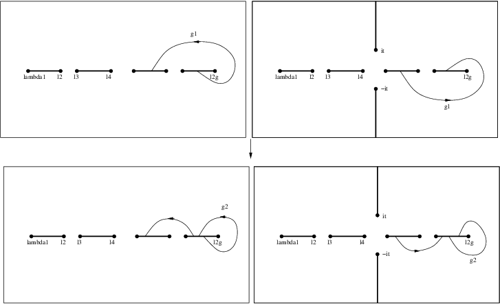
For a point $z$ in $\mathcal{L}_{1}$ ( $\mathcal{L}_{2}$ ), the contour of integration $\Sigma_{1}$ goes from $\lambda_{2g+2}$ to $z$ in $\mathcal{L}_{1}$ ( $\mathcal{L}_{2}$ ) without intersecting $(-\infty,\lambda_{2g+2})$ and the branch cuts on the imaginary axis. For a point $z$ in the upper (lower) half plane in $\mathcal{L}_{3}$ , the contour of integration $\Sigma_{3}$ consists of 2 parts. The first part lies in $\mathcal{L}_{2}$ , goes from $\lambda_{2g+2}$ to a point $i\zeta$ ( $-i\zeta$ ) on the branch cut in the imaginary axis without intersecting $(-\infty,\lambda_{2g+2})$ in $\mathcal{L}_{2}$ and enter the branch cut from the left hand side of this point. The second part lies in the upper (lower) half plane in $\mathcal{L}_{3}$ , goes from the right hand side of $i\zeta$ ( $-i\zeta$ ) to the point $z$ . For a point $z$ in the upper (lower) half plane in $\mathcal{L}_{4}$ , the contour of integration consists of 3 parts. The first part lies in $\mathcal{L}_{2}$ , goes from $\lambda_{2g+2}$ to a point $-i\zeta$ ( $i\zeta$ ) on the branch cut in the imaginary axis without intersecting $(-\infty,\lambda_{2g+2})$ in $\mathcal{L}_{2}$ and enter the branch cut from the left hand side of this point. The second part lies in the lower (upper) half plane in $\mathcal{L}_{3}$ , goes from the right hand side of $-i\zeta$ ( $i\zeta$ ) to the origin. The last part lies in the upper (lower) half plane in $\mathcal{L}_{4}$ , goes from the origin to the point $z$ . The choice of the point $\pm i\zeta$ in the construction is immaterial as long as it lies on the branch cut on the imaginary axis.

Let $z^{j}$ be the point on $\mathcal{L}_{j}$ that projects to $z$ in $\overline{\mathbb{C}}$ and $\vec{A}$ be a $g$ -dimensional constant vector. We can now define four functions $\theta^{j}(u(z)+\vec{A})$ on the complex $z$ -plane by

\theta^{j}(u(z)+\vec{A})=\theta(u(z^{j})+\vec{A}).

(4.12)

These functions will have jump discontinuities in the complex $z$ -plane. By using the periodicity of the theta function (4.7), we can compute their jump discontinuities.

Proposition 3.

Let $\vec{A}=(A_{1},\ldots,A_{g})^{T}$ be a $g$ dimensional vector. The functions $\theta^{j}(u(z)+\vec{A})$ are analytic in $\mathbb{C}\setminus(\mathbb{R}\cup S_{\sigma-\mu_{2}})$ . On $\mathbb{R}\cup S_{\sigma-\mu_{2}}$ , they satisfy the following conditions

\begin{split}\theta_{\pm}^{1}(u(z)+\vec{A})&=\theta_{\mp}^{2}(u(z)+\vec{A}),\quad z\in\Xi_{j},\quad j=1,\ldots,g+1,\\ \theta_{+}^{l}(u(z)+\vec{A})&=\theta_{-}^{l}(u(z)+\vec{A})e^{(-1)^{l}2\pi i\left(u_{j}(z)+A_{j}+\frac{\Pi_{jj}}{2}\right)},\quad z\in\tilde{\Xi}_{j},\quad j=1,\ldots,g,\quad l=1,2,\\ \theta_{+}^{l}(u(z)+\vec{A})&=\theta_{-}^{l}(u(z)+\vec{A}),\quad z\in\left(\tilde{\Xi}_{0}\cup\tilde{\Xi}_{g+1}\right),\quad l=1,2,\\ \theta^{2}_{\pm}(u(z)+\vec{A})&=\theta^{3}_{\mp}(u(z)+\vec{A}),\quad z\in S_{\sigma-\mu_{2}},\\ \theta^{3}_{\pm}(u(z)+\vec{A})&=\theta^{4}_{\mp}(u(z)+\vec{A}),\quad z\in\mathbb{R},\\ \theta^{l}_{+}(u(z)+\vec{A})&=\theta^{l}_{-}(u(z)+\vec{A}),\quad z\in S_{\sigma-\mu_{2}},\quad l=1,4.\end{split}

(4.13)

Proof.

Let us first consider the discontinuities of $\theta^{1}(u(z)+\vec{A})$ and $\theta^{2}(u(z)+\vec{A})$ across $\Xi_{j}$ . Let $\pi:\mathcal{L}\rightarrow\overline{\mathbb{C}}$ be the projection of $\mathcal{L}$ onto the Riemann sphere. Suppose $z$ is a point in $\Xi_{j}$ . Let $z\in\mathbb{C}$ and define the points $z_{\pm\epsilon}^{j}\in\mathcal{L}_{j}$ to be

\pi(z_{\pm i\epsilon}^{j})=z\pm i\epsilon,\quad z_{\pm i\epsilon}^{j}\in\mathcal{L}_{j}.

(4.14)

We will now choose $\epsilon>0$ to be real and positive and let $z\in\Xi_{j}$ . From the definition of the integration contour in Figure 3 and the canonical basis of cycles in Figure 2, we have the following relation between the points $z_{\pm i\epsilon}^{j}$ as $\epsilon\rightarrow 0$ .

\begin{split}u(z_{\pm i\epsilon}^{1})&=u(z_{\mp i\epsilon}^{2}),\quad z\in\Xi_{g+1},\\ u(z_{\pm i\epsilon}^{1})&=u(z_{\mp i\epsilon}^{2})+\sum_{k=j}^{g}\oint_{a_{k}}\mathrm{d}\omega,\\ &=u(z_{\mp i\epsilon}^{2})+\sum_{k=j}^{g}\vec{e}^{k},\quad z\in\Xi_{j},\quad j=1,\ldots,g.\end{split}

(4.15)

where $\vec{e}^{k}$ is a vector with 1 in the $k^{th}$ entry and zero elsewhere and $\mathrm{d}\omega$ is the vector

\mathrm{d}\omega=(\mathrm{d}\omega_{1},\ldots,\mathrm{d}\omega_{g})^{T}.

(4.16)

From this and the periodicity of the theta function (4.7), we obtain

\theta_{\pm}^{1}(u(z)+\vec{A})=\theta_{\mp}^{2}(u(z)+\vec{A}),\quad z\in\Xi_{j},\quad j=1,\ldots,g+1.

(4.17)

Let us now consider a point $z$ in $\tilde{\Xi}_{j}$ . Again, from the definition of the integration contour and the canonical basis, we have, as $\epsilon\rightarrow 0$ , the following

\begin{split}u(z_{i\epsilon}^{l})&=u(z_{-i\epsilon}^{l})+(-1)^{l+1}\oint_{b_{j}}\mathrm{d}\omega,\\ &=u(z_{-i\epsilon}^{l})+(-1)^{l+1}\Pi\vec{e}^{j},\quad z\in\tilde{\Xi}_{j},\quad j=1,\ldots,g.\end{split}

(4.18)

where $l=1,2$ . From this and the periodicity of the theta function, we see that

\begin{split}\theta_{+}^{l}(u(z)+\vec{A})&=\theta_{-}^{l}(u(z)+\vec{A})e^{(-1)^{l}2\pi i\left(u_{j}(z)+A_{j}+\frac{\Pi_{jj}}{2}\right)},\quad z\in\tilde{\Xi}_{j},\quad j=1,\ldots,g.\end{split}

(4.19)

From the definition of the integration contour, it is clear that $\theta^{1}(u(z)+\vec{A})$ and $\theta^{2}(u(z)+\vec{A})$ are analytic across $\mathbb{R}\setminus\left(\lambda_{1},\lambda_{2g+2}\right)$ and that $\theta^{1}(u(z)+\vec{A})$ is analytic across $S_{\sigma-\mu_{2}}$ .

Let us now consider the discontinuities of $\theta^{3}(u(z)+\vec{A})$ and $\theta^{2}(u(z)+\vec{A})$ on $S_{\sigma-\mu_{2}}$ . Let $z$ be a point on $S_{\sigma-\mu_{2}}$ , from the definition of the contours, it follows immediately that

\begin{split}\theta_{+}^{2}(u(z)+\vec{A})&=\theta_{-}^{3}(u(z)+\vec{A}),\quad z\in S_{\sigma-\mu_{2}}.\end{split}

(4.20)

Let us now consider the boundary value of $\theta^{2}(u(z)+\vec{A})$ on the minus side of $S_{\sigma-\mu_{2}}$ . For small and positive $\epsilon\rightarrow 0$ , we have

\begin{split}u(z^{2}+\epsilon)+\oint_{\Sigma}\mathrm{d}\omega&=u(z^{3}-\epsilon),\end{split}

(4.21)

where $\Sigma$ is the close loop on $\mathcal{L}$ depicted in Figure 4. Since this loop is contractible, we have

\begin{split}\theta_{-}^{2}(u(z)+\vec{A})&=\theta_{+}^{3}(u(z)+\vec{A}),\quad z\in S_{\sigma-\mu_{2}}.\end{split}

(4.22)

Finally, the conditions

\begin{split}\theta^{3}_{\pm}(u(z)+\vec{A})&=\theta^{4}_{\mp}(u(z)+\vec{A}),\quad z\in\mathbb{R},\\ \theta^{4}_{+}(u(z)+\vec{A})&=\theta^{4}_{-}(u(z)+\vec{A}),\quad z\in S_{\sigma-\mu_{2}}.\end{split}

(4.23)

follow directly from the definition of the contour of integration. ∎

4.2 Meromorphic differentials

Another key ingredient in the construction of the parametrix is meromorphic differentials on the Riemann surface. Most of the results that we will be using can be found in [24].

Proposition 4.

Let $d_{1},\ldots,d_{k}$ be $k$ distinct points on a Riemann surface $\mathcal{L}$ . Let $c_{1},\ldots,c_{k}$ be complex numbers with $\sum_{j=1}^{k}c_{k}=0$ . Then there exists a meromorphic 1-form $\mathrm{d}\Omega$ on $\mathcal{L}$ , holomorphic on $\mathcal{L}\setminus\{d_{1},\ldots,d_{k}\}$ such that

\mathrm{d}\Omega(x)=\left(\frac{c_{j}}{x_{j}}+O(1)\right)dx_{j},\quad x\rightarrow d_{j},\quad j=1,\ldots,k.

(4.24)

where $x_{j}$ is a local coordinate near $d_{j}$ such that $x_{j}=0$ at $d_{j}$ .

This result can be found for example, in [24]. (p.52, theorem II.5.3)

A meromorphic 1-form with simple poles only is called a meromorphic 1-form of the third type. Let $\mathrm{d}\Omega$ be a meromorphic 1-form of the third type. In order to define the periods of $\mathrm{d}\Omega$ unambiguously, one has to define the periods to be integrals around close loops $\hat{a}_{j}$ and $\hat{b}_{j}$ that are homologic to the $a$ and $b$ -cycles in Figure 2 in $\mathcal{L}\setminus\Omega_{pole}$ , where $\Omega_{pole}$ is the set of poles of $\mathrm{d}\Omega$ .

By adding suitable multiples of holomorphic 1-forms to a given meromorphic 1-form, we can obtain meromorphic 1-forms with arbitrary $a$ -periods. For example, if a meromorphic 1-form given by Proposition 4 has the following $a$ -periods

\oint_{a_{j}}\mathrm{d}\Omega=\mathcal{A}_{j},\quad j=1,\ldots,g.

Then the meromorphic 1-form

\mathrm{d}\tilde{\Omega}=\mathrm{d}\Omega+\sum_{j=1}^{g}(\tilde{\mathcal{A}}_{j}-\mathcal{A}_{j})\mathrm{d}\omega_{j}

will have $a$ -periods

\oint_{a_{j}}\mathrm{d}\tilde{\Omega}=\tilde{\mathcal{A}}_{j},\quad j=1,\ldots,g.

but with the same pole structure and residues. Of course, we can not control both the $a$ and the $b$ -periods of the 1-form. In fact, meromorphic 1-forms with prescribed $a$ -period and pole structure is uniquely defined. A meromorphic 1-form with all $a$ -periods zero is called a normalized meromorphic 1-form.

Proposition 5.

Let $d_{1},\ldots,d_{k}$ be $k$ distinct points on a Riemann surface $\mathcal{L}$ . Let $c_{1},\ldots,c_{k}$ be complex numbers with $\sum_{j=1}^{k}c_{k}=0$ and let $\mathcal{A}_{1},\ldots,\mathcal{A}_{g}$ be arbitrary complex numbers. Then there exists a unique meromorphic 1-form of the third type $\mathrm{d}\Omega$ on $\mathcal{L}$ , holomorphic on $\mathcal{L}\setminus\{d_{1},\ldots,d_{k}\}$ such that

\begin{split}\mathrm{Res}_{z=d_{j}}\mathrm{d}\Omega=c_{j},\quad j=1,\ldots,k,\\ \oint_{a_{j}}\mathrm{d}\Omega=\mathcal{A}_{j},\quad j=1,\ldots,g.\end{split}

(4.25)

Proof.

We have already shown the existence part. To see the uniqueness part, let $\mathrm{d}\Omega$ and $\mathrm{d}\Omega^{\prime}$ be 2 meromorphic 1-forms of the third type with the properties (4.25). Let $\mathrm{d}\tilde{\Omega}$ be their difference. Then, since both $\mathrm{d}\Omega$ and $\mathrm{d}\Omega^{\prime}$ have the same singular behavior at the points $d_{j}$ , the 1-form $\mathrm{d}\tilde{\Omega}$ does not have any pole and is therefore holomorphic. Moreover, all its $a$ -periods vanish. Since a holomorphic 1-form with vanishing $a$ -periods has to be zero itself, (See, for example, [24], p.65, Proposition III.3.3) the proposition is proven. ∎

We will conclude this section with a result that relates the periods of a normalized meromorphic 1-form to the values of the Abel map at its poles.

Theorem 6.

(See e.g. [24], p.65, III.3) Let $\eta$ be a meromorphic differential of the third type with simple poles at the points $d_{i}\in\mathcal{L}$ and $\tilde{\eta}$ be a holomorphic differential. Let $\Pi^{i}$ and $\tilde{\Pi}^{i}$ be their periods

\begin{split}\int_{a_{i}}\eta&=\Pi^{i},\quad\int_{b_{i}}\eta=\Pi^{i+g}\\ \int_{a_{i}}\tilde{\eta}&=\tilde{\Pi}^{i},\quad\int_{b_{i}}\tilde{\eta}=\tilde{\Pi}^{i+g}\end{split}

(4.26)

Then the Riemann bilinear relation is the following

\sum_{i=1}^{g}\tilde{\Pi}^{i}\Pi^{i+g}-\tilde{\Pi}^{g+i}\Pi^{i}=2\pi i\sum_{d_{i}}\mathrm{Res}_{d_{i}}(\eta)\int_{x_{0}}^{d_{i}}\tilde{\eta},

(4.27)

where $x_{0}$ is an arbitrary point on $\mathcal{L}$ .

5 Construction of the outer parametrix

We will now construct the local parametrix with the the theta function and meromorphic 1-forms.

Let us now define a local coordinate $w$ near $\infty^{2}$ , the point on $\mathcal{L}_{2}$ , $\mathcal{L}_{3}$ and $\mathcal{L}_{4}$ that projects onto $\infty$ in the Riemann sphere.

\begin{split}w&=\left\{\begin{array}[]{ll}z^{-\frac{1}{3}},&\hbox{in the first and fourth quadrants of $\mathcal{L}_{2}$;}\\ \omega^{2}z^{-\frac{1}{3}},&\hbox{in the second quadrant of $\mathcal{L}_{2}$;}\\ \omega z^{-\frac{1}{3}},&\hbox{in the third quadrant of $\mathcal{L}_{2}$.}\end{array}\right.\\ w&=\left\{\begin{array}[]{ll}\omega^{2}z^{-\frac{1}{3}},&\hbox{in the first quadrant of $\mathcal{L}_{3}$;}\\ z^{-\frac{1}{3}},&\hbox{in the second and third quadrants of $\mathcal{L}_{3}$;}\\ \omega z^{-\frac{1}{3}},&\hbox{in the fourth quadrant of $\mathcal{L}_{3}$.}\end{array}\right.\\ w&=\left\{\begin{array}[]{ll}\omega z^{-\frac{1}{3}},&\hbox{in the first and second quadrants of $\mathcal{L}_{4}$;}\\ \omega^{2}z^{-\frac{1}{3}},&\hbox{in the third and fourth quadrants of $\mathcal{L}_{4}$.}\end{array}\right.\end{split}

(5.1)

where $\omega=e^{\frac{2\pi i}{3}}$ and the branch of $z^{\frac{1}{3}}$ is chosen such that $\arg z\in(-\pi,\pi)$ . One can check that $w$ is indeed holomorphic in $\mathcal{L}$ in a neighborhood of $\infty^{2}$ .

Let us now define four meromorphic 1-forms of the third type $\mathrm{d}\Delta_{j}$ , $j=1,\ldots,4$ by the following properties.

Definition 3.

The normalized meromorphic 1-forms $\mathrm{d}\Delta_{j}$ are holomorphic in

\mathcal{L}\setminus\{\pm it,\lambda_{1}^{1},\ldots,\lambda_{2g+2}^{1},\iota_{1},\ldots,\iota_{g},\infty^{1},\infty^{2}\}.

where $\pm it$ are the points in $\mathcal{L}_{2}$ that project onto $\pm ic$ and $\iota_{k}$ are the zeros of $\theta(u(x))$ . At these points they have simple poles with residues

\begin{split}\mathrm{Res}_{\lambda_{k}^{1}}\mathrm{d}\Delta_{j}&=\mathrm{Res}_{\pm it}\mathrm{d}\Delta_{j}=-\frac{1}{2},\quad k=1,\ldots,2g+2,\\ \mathrm{Res}_{\iota_{k}}\mathrm{d}\Delta_{j}&=1,\quad k=1,\ldots,g,\\ \mathrm{Res}_{\infty^{1}}\mathrm{d}\Delta_{1}&=0,\quad\mathrm{Res}_{\infty^{2}}\mathrm{d}\Delta_{1}=2,\\ \mathrm{Res}_{\infty^{1}}\mathrm{d}\Delta_{2}&=3,\quad\mathrm{Res}_{\infty^{2}}\mathrm{d}\Delta_{2}=-1,\\ \mathrm{Res}_{\infty^{1}}\mathrm{d}\Delta_{3}&=2,\quad\mathrm{Res}_{\infty^{2}}\mathrm{d}\Delta_{1}=0,\\ \mathrm{Res}_{\infty^{1}}\mathrm{d}\Delta_{4}&=1,\quad\mathrm{Res}_{\infty^{2}}\mathrm{d}\Delta_{4}=1,\end{split}

(5.2)

provided none of the $\iota_{l}$ is equal to $\lambda_{k}^{1}$ for some $k$ . If some $\iota_{l}$ is equal to $\lambda_{k}^{1}$ for some $k$ , then the residue at $\iota_{l}$ will be $\frac{1}{2}$ .

These 1-forms are then uniquely defined. We will denote the $b$ -period of these 1-forms by $\beta_{j}$ .

\beta_{j}=\left(\oint_{b_{1}}\mathrm{d}\Delta_{j},\ldots,\oint_{b_{g}}\mathrm{d}\Delta_{j}\right)^{T},\quad j=1,\ldots,4.

(5.3)

To avoid ambiguity in the $b$ -periods, let $\pi(\iota_{k})$ be the projection of $\iota_{k}$ on $\tilde{\Xi}_{k}$ (See remark 2). Then the $b$ -periods are computed as integrals on $b$ -cycles in $\mathcal{L}_{1}$ that intersects $\tilde{\Xi}_{k}$ at any point $x<\pi(\iota_{k})$ if $\pi(\iota_{k})\neq\lambda_{2k}$ . If $\pi(\iota_{k})=\lambda_{2k}$ , then the $b$ -cycle can intersect $\tilde{\Xi}_{k}$ at any point $x\neq\lambda_{2k}$ in $\mathcal{L}_{1}$ .

We will now define four functions in the Riemann surface $\mathcal{L}$ . First let $\Xi_{k}^{\pm}\in\mathcal{L}$ be the images of $\Xi_{k}$ under the maps $\xi_{1,\pm}(z)$ , that is,

\begin{split}\Xi_{k}^{\pm}=\left\{(z,\xi)|z\in\Xi_{k},\quad\xi=\xi_{1,\pm}(z)\right\},\quad k=1,\ldots,g+1.\end{split}

(5.4)

Let $z_{0}$ be a point in $\Xi_{g+1}^{-}$ . The exact choice of $z_{0}$ is immaterial to the construction as long as $z_{0}\neq\lambda_{2g+1}^{1}$ or $\lambda_{2g+2}^{1}$ . We will now define the functions $N_{j}(z)$ on $\mathcal{L}$ as follows.

\begin{split}N_{j}(z)&=e^{\Delta_{j}(z)}\frac{\theta\left(u(z)+\frac{\beta_{j}}{2\pi i}+n\vec{\alpha}\right)}{\theta\left(u(z)\right)}\\ &=e^{\Delta_{j}(z)}\Theta_{j}(z),\quad\vec{\alpha}=\left(\alpha_{1},\ldots,\alpha_{g}\right)^{T},\quad j=1,\ldots,4.\end{split}

(5.5)

where the function $\Delta_{j}(z)$ is given by $\Delta_{j}(z)=\int_{z_{0}}^{z}\mathrm{d}\Delta_{j}$ and the path of integration is defined in the same way as the ones for the Abel map, except that every path now starts at $z_{0}$ .

Let $z^{k}$ be the point on $\mathcal{L}_{k}$ that projects to $z$ in $\overline{\mathbb{C}}$ . As before, we will now define four functions $e^{\Delta_{j}^{k}(z)}$ on the complex $z$ -plane by

e^{\Delta_{j}^{k}(z)}=e^{\Delta_{j}(z^{k})}.

(5.6)

Then these functions have the following jump discontinuities in the complex $z$ -plane.

Proposition 6.

The functions $e^{\Delta_{j}^{l}(z)}$ are analytic in $\mathbb{C}\setminus(\mathbb{R}\cup S_{\sigma-\mu_{2}})$ . On $\mathbb{R}\cup S_{\sigma-\mu_{2}}$ , they satisfy the following conditions

\begin{split}e^{\Delta_{j,\pm}^{1}(z)}&=\mp e^{\Delta_{j,\mp}^{2}(z)},\quad z\in\Xi_{k},\quad k=1,\ldots,g+1,\\ e^{\Delta_{j,+}^{l}(z)}&=e^{\Delta_{j,-}^{l}(z)+(-1)^{l-1}\left(\beta_{j}\right)_{k}},\quad z\in\tilde{\Xi}_{k},\quad k=1,\ldots,g,\quad l=1,2,\\ e^{\Delta_{j,+}^{l}(z)}&=e^{\Delta_{j,-}^{l}(z)},\quad z\in\left(\tilde{\Xi}_{0}\cup\tilde{\Xi}_{g+1}\right),\quad l=1,2,\\ e^{\Delta_{j,\pm}^{2}(z)}&=\pm e^{\Delta_{j,\mp}^{3}(z)},\quad z\in S_{\sigma-\mu_{2}},\\ e^{\Delta_{j,\pm}^{3}(z)}&=e^{\Delta_{j,\mp}^{4}(z)},\quad z\in\mathbb{R},\\ e^{\Delta_{j,+}^{l}(z)}&=e^{\Delta_{j,-}^{l}(z)},\quad z\in S_{\sigma-\mu_{2}},\quad l=1,4.\end{split}

(5.7)

where $\left(\beta_{j}\right)_{k}$ is the $k^{th}$ component of the vector $\beta_{j}$ .

Proof.

The proof follows similar argument as the ones used in the proof of Proposition 3. First let us consider the jump discontinuities on $\Xi_{k}$ . Let $z$ be a point in $\Xi_{k}$ and define the points $z_{\pm i\epsilon}^{l}$ as in (4.14) in the proof of Proposition 3. First consider the boundary values $e^{\Delta_{j,+}^{1}(z)}$ and $e^{\Delta_{j,-}^{2}(z)}$ . Choose integration contours $\Sigma_{+}$ and $\Sigma_{-}$ from $z_{0}$ to the points $z_{i\epsilon}^{1}$ and $z_{-i\epsilon}^{2}$ as in Figure 5. Let $\Sigma=\Sigma_{+}-\Sigma_{-}$ . Then $\Sigma$ can be deformed into the sum $\sum_{l=k}^{g}a_{l}$ of the $a$ -cycles and a loop $\Sigma_{2g+2}$ around the point $\lambda_{2g+2}^{1}$ in $\mathcal{L}\setminus\Delta_{pole}$ , where $\Delta_{pole}$ is the set of poles of $\mathrm{d}\Delta_{j}$ . (See Figure 6).

\Delta_{pole}=\{\pm it,\lambda_{1}^{1},\ldots,\lambda_{2g+2}^{1},\iota_{1},\ldots,\iota_{g},\infty^{1},\infty^{2}\}.

(5.8)

Therefore we have

\begin{split}\exp\left(\Delta_{j}(z_{i\epsilon}^{1})\right)&=\exp\left(\Delta_{j}(z_{-i\epsilon}^{2})+\sum_{l=k}^{g}\oint_{a_{l}}\mathrm{d}\Delta_{j}+\oint_{\Sigma_{2g+2}}\mathrm{d}\Delta_{j}\right),\\ &=-\exp\left(\Delta_{j}(z_{-i\epsilon}^{2})\right),\quad z\in\Xi_{k},\quad k=1,\ldots,g.\end{split}

(5.9)

where the last equality follows from the fact that $\mathrm{d}\Delta_{j}$ has residue $-\frac{1}{2}$ at the point $\lambda_{2g+2}^{1}$ .

Let us now consider the boundary values $e^{\Delta_{j,-}^{1}(z)}$ and $e^{\Delta_{j,+}^{2}(z)}$ on $\Xi_{k}$ . Since $z_{0}\in\Xi_{g+1}^{-}$ , the integration contours $\Sigma_{-}$ and $\Sigma_{+}$ can now be chosen to lie in the lower (upper) half plane of $\mathcal{L}_{1}$ ( $\mathcal{L}_{2}$ ). The loop $\Sigma=\Sigma_{+}-\Sigma_{-}$ can now be deformed into the sum $-\sum_{l=k}^{g}a_{l}$ of the $a$ -cycles. However, such a deformation will necessarily go pass the poles $\lambda_{2k}^{1},\ldots,\lambda_{2g+1}^{1}$ and $\iota_{k},\ldots,\iota_{g}$ of $\mathrm{d}\Delta_{j}$ (Recall that by the remark after Proposition 2, there is exactly one point $\iota_{k}$ that belongs to $\tilde{\Xi}_{k}^{1}\cup\tilde{\Xi}_{k}^{2}$ ). Since the residues of $\mathrm{d}\Delta_{j}$ at these points are given by $-\frac{2(g-k)}{2}$ from the $\lambda_{l}^{1}$ and $g-k$ from the $\iota_{l}$ when all $\iota_{l}$ and $\lambda_{m}^{1}$ are distinct, the total residue at these points is zero. It is clear from Definition 3 that, when some $\iota_{l}$ coincide with the $\lambda_{m}^{1}$ , the total residue at these points remains unchanged. Hence we have

\begin{split}\exp\left(\Delta_{j}(z_{-i\epsilon}^{1})\right)&=\exp\left(\Delta_{j}(z_{i\epsilon}^{2})-\oint_{\Sigma}\mathrm{d}\Delta_{j}\right),\\ &=\exp\left(\Delta_{j}(z_{i\epsilon}^{2})\right),\quad z\in\Xi_{k},\quad k=1,\ldots,g.\end{split}

Let us now consider the boundary values on the gaps $\tilde{\Xi}_{k}$ . Let $z\in\tilde{\Xi}_{k}$ . For the boundary values $e^{\Delta_{j,\pm}^{1}(z)}$ , we choose $\Sigma_{\pm}$ to be integration contours that go from $z_{0}$ to $z_{\pm i\epsilon}^{1}$ in $\mathcal{L}_{1}$ without intersecting $(-\infty,\lambda_{2g+2}^{1})$ except at $z_{0}$ and $z_{\pm i\epsilon}^{1}$ . Let the loop $\Sigma$ be $\Sigma=\Sigma_{+}-\Sigma_{-}$ , then for $k=1,\ldots,g$ , $\Sigma$ can be deformed into the $b$ -cycle $b_{k}$ without passing any pole of $\mathrm{d}\Delta_{j}$ , except possibly $\iota_{k}$ (Recall the definition of the $b$ -periods of $\mathrm{d}\Delta_{j}$ in Definition 3). When $\iota_{k}$ is not equal to $\lambda_{2k}^{1}$ or $\lambda_{2k+1}^{1}$ , $\mathrm{d}\Delta_{j}$ has integer residue at $\iota_{k}$ , and when $\iota_{k}$ is equal to either $\lambda_{2k}^{1}$ or $\lambda_{2k+1}^{1}$ , the deformation from $\Sigma$ to $b_{k}$ will not have to go pass $\iota_{k}$ . This implies

e^{\Delta_{j,+}^{1}(z)}=e^{\Delta_{j,-}^{1}(z)+\left(\beta_{j}\right)_{k}},\quad z\in\tilde{\Xi}_{k},\quad k=1,\ldots,g.

For $k=0$ , the loop $\Sigma$ can be deformed into a small loop around the point $\infty^{1}$ . Since the 1-forms $\mathrm{d}\Delta_{j}$ have integer residues at $\infty^{1}$ , we have

e^{\Delta_{j,+}^{1}(z)}=e^{\Delta_{j,-}^{1}(z)},\quad z\in\tilde{\Xi}_{0}.

If $k=g+1$ , then the loop $\Sigma$ will be contractible in $\mathcal{L}\setminus\Delta_{pole}$ . Hence we have

e^{\Delta_{j,+}^{1}(z)}=e^{\Delta_{j,-}^{1}(z)},\quad z\in\tilde{\Xi}_{g+1}.

On the other hand, for the boundary values $e^{\Delta_{j,\pm}^{2}(z)}$ on $\tilde{\Xi}_{k}$ , let us consider $\Sigma_{\pm}$ to be integration contours that go from $z_{0}$ to $z_{\pm i\epsilon}^{2}$ in $\mathcal{L}_{2}$ without intersecting $(-\infty,\lambda_{2g+2}^{1})$ except at $z_{0}$ and $z_{\pm i\epsilon}^{2}$ . Let $k=1,\ldots,g$ , and let $\pi(\iota_{k})$ be the projection of $\iota_{k}$ onto the $z$ -plane. Then depending on the relative positions of $z$ , $\pi(\iota_{k})$ and $\lambda_{2k}^{1}$ , the loop $\Sigma=\Sigma_{+}-\Sigma_{-}$ can be deformed into $-b_{k}$ , together with small loops around the poles $\iota_{k},\ldots,\iota_{g}$ and $\lambda_{2k+1}^{1},\ldots,\lambda_{2g+2}^{1}$ in $\mathcal{L}\setminus\Delta_{pole}$ ; or it can be deformed into the sum of $-b_{k}$ and small loops around the poles $\iota_{k+1},\ldots,\iota_{g}$ and $\lambda_{2k+1}^{1},\ldots,\lambda_{2g+2}^{1}$ in $\mathcal{L}\setminus\Delta_{pole}$ . In either cases, the total residue of $\mathrm{d}\Delta_{j}$ at these points will be an integer. Therefore we have

e^{\Delta_{j,+}^{2}(z)}=e^{\Delta_{j,-}^{2}(z)-\left(\beta_{j}\right)_{k}},\quad z\in\tilde{\Xi}_{k},\quad k=1,\ldots,g.

Similarly, for $k=0$ , the loop $\Sigma$ can be deformed into a small loop around the points $\infty^{2}$ and $\pm it$ . Since the total residue the 1-form $\mathrm{d}\Delta_{j}$ at these points is an integer, we have

e^{\Delta_{j,+}^{2}(z)}=e^{\Delta_{j,-}^{2}(z)},\quad z\in\tilde{\Xi}_{0}.

If $k=g+1$ , then the loop $\Sigma$ will be contractible in $\mathcal{L}\setminus\Delta_{pole}$ . Hence we have

e^{\Delta_{j,+}^{2}(z)}=e^{\Delta_{j,-}^{2}(z)},\quad z\in\tilde{\Xi}_{g+1}.

We now consider the boundary values $e^{\Delta_{j,-}^{2}(z)}$ and $e^{\Delta_{j,+}^{3}(z)}$ at $S_{\sigma-\mu_{2}}$ , let $z\in S_{\sigma-\mu_{2}}$ . Let us again denote by $\Sigma_{+}$ and $\Sigma_{-}$ contours of integration from $z_{0}$ to $z-\epsilon$ in $\mathcal{L}_{3}$ and $z+\epsilon$ in $\mathcal{L}_{2}$ . Then depending on whether $z$ is in the upper or lower half plane, the loop $\Sigma=\Sigma_{+}-\Sigma_{-}$ can be deformed into to a small loop around the pole $it$ or $-it$ in $\mathcal{L}\setminus\Delta_{pole}$ (See Figure 4. The loop $\Sigma$ in this case is the same except that it begins and ends at $z_{0}$ instead of $\lambda_{2g+2}^{1}$ ). Since the residue of $\mathrm{d}\Delta_{j}$ around $it$ or $-it$ is $-\frac{1}{2}$ , we have

e^{\Delta_{j,+}^{3}(z)}=-e^{\Delta_{j,-}^{2}(z)},\quad z\in S_{\sigma-\mu_{2}}.

(5.10)

The rest of the jump discontinuities in (5.7) now follow directly from the definition of the integration contours as in the proof of Proposition 3. ∎

Let us denote by $N_{j}^{k}(z)$ the projection of $N_{j}(z)$ onto the $k^{th}$ -sheet, that is, $N_{j}^{k}(z)=N_{j}(z^{k})=N_{j}\left(z,\xi_{k}(z)\right)$ , where $\xi_{k}(z)$ is the function $\xi(z)$ on $\mathcal{L}_{k}$ . Then we have the following.

Theorem 7.

Let $N(z)$ be the $4\times 4$ matrix whose elements are given by

N_{jk}(z)=\left\{\begin{array}[]{ll}N_{j}^{k}(z),&\hbox{$\mathrm{Im}z>0$;}\\ (-1)^{\delta_{4,k}}N_{j}^{k}(z),&\hbox{$\mathrm{Im}z<0$,}\end{array}\right.

(5.11)

where $N_{j}(z)$ are defined in (5.5). Suppose we have

\theta\left(u(\infty^{1})+\frac{\beta_{j}}{2\pi i}+n\vec{\alpha}\right)\theta\left(u(\infty^{2})+\frac{\beta_{j}}{2\pi i}+n\vec{\alpha}\right)\neq 0.

(5.12)

Let the constants $L_{j}$ be

\begin{split}L_{1}&=N_{1}^{-1}(\infty^{1}),\quad L_{2}=\lim_{w\rightarrow 0}N_{2}^{-1}(w)w^{-1},\\ L_{3}&=\lim_{w\rightarrow 0}N_{3}^{-1}(w),\quad L_{4}=\lim_{w\rightarrow 0}N_{4}^{-1}(w)w,\end{split}

(5.13)

where $w$ is the local coordinate near $\infty^{2}$ defined in (5.1) and the limits in $L_{2}$ , $L_{3}$ and $L_{4}$ are taken as $z\rightarrow\infty^{2}$ in the first quadrant of $\mathcal{L}_{2}$ . Then the matrix

S_{\infty}(z)=\begin{pmatrix}1&0&0&0\\ 0&-\frac{i}{\sqrt{3}}&0&-\frac{i\kappa}{\sqrt{3}}\\ 0&0&-\frac{i}{\sqrt{3}}&0\\ 0&0&0&-\frac{i}{\sqrt{3}}\end{pmatrix}\diag\left(L_{1},L_{2},L_{3},L_{4}\right)N(z)

(5.14)

satisfies the Riemann-Hilbert problem (3.7), where $\kappa$ is the following in the expansion of $N_{2}(z)$ at $z=\infty^{2}$

N_{2}(z)=L_{2}^{-1}\left(w^{-1}+\kappa_{2,0}-\kappa w+O(w^{2})\right),

as $z\rightarrow\infty^{2}$ in the first quadrant of $\mathcal{L}_{2}$ .

Remark 3.

The constants $L_{j}$ , $j=1,\ldots,4$ can be represented as

\begin{split}L_{1}&=e^{-\Delta_{1}(\infty^{1})}\frac{\theta\left(u(\infty^{1})\right)}{\theta\left(u(\infty^{1})+\frac{\beta_{1}}{2\pi i}+n\vec{\alpha}\right)},\\ L_{2}&=\left(\lim_{w\rightarrow 0}e^{-\Delta_{2}(w)}w^{-1}\right)\frac{\theta\left(u(\infty^{2})\right)}{\theta\left(u(\infty^{2})+\frac{\beta_{2}}{2\pi i}+n\vec{\alpha}\right)},\\ L_{3}&=\lim_{w\rightarrow 0}e^{-\Delta_{3}(w)}\frac{\theta\left(u(\infty^{2})\right)}{\theta\left(u(\infty^{2})+\frac{\beta_{3}}{2\pi i}+n\vec{\alpha}\right)},\\ L_{4}&=\left(\lim_{w\rightarrow 0}e^{-\Delta_{4}(w)}w\right)\frac{\theta\left(u(\infty^{2})\right)}{\theta\left(u(\infty^{2})+\frac{\beta_{4}}{2\pi i}+n\vec{\alpha}\right)}.\end{split}

(5.15)

where the limits are taken as $z\rightarrow\infty^{2}$ in the first quadrant of $\mathcal{L}_{2}$ .

Proof.

First note that, by using Proposition 3 and Proposition 6, one can verify that $N(z)$ does satisfy the jump discontinuities in (3.7).

Since $N(z)$ satisfies the jump discontinuities of (3.7), the matrix $M(z)N^{-1}(z)$ does not have any jump discontinuities in $\mathbb{C}$ . Moreover, this matrix does not grow faster than $z^{\frac{2}{3}}$ at $z=\infty$ and has at worst square root singularities at the points $\lambda_{j}$ and $\pm it$ . Since it has no jump discontinuities, all these singularities are removable and therefore we have $M(z)=HN(z)$ for some constant matrix $H$ . To determine the constant matrix $H$ , we will have to study the behavior of $N(z)$ as $z\rightarrow\infty$ .

The behavior of $M(z)$ is given by the following

M(z)=\begin{pmatrix}1+O(z^{-1})&O(z^{-\frac{2}{3}})&O(z^{-\frac{2}{3}})&O(z^{-\frac{2}{3}})\\ O(z^{-1})&*&*&*\\ O(z^{-1})&*&*&*\\ O(z^{-1})&*&*&*\end{pmatrix}

(5.16)

where the $3\times 3$ lower right block is given by

\begin{pmatrix}-\frac{i}{\sqrt{3}}z^{\frac{1}{3}}(1+O(z^{-1}))&\frac{\omega i}{\sqrt{3}}z^{\frac{1}{3}}(1+O(z^{-1}))&\frac{\omega^{2}i}{\sqrt{3}}z^{\frac{1}{3}}(1+O(z^{-1}))\\ -\frac{i}{\sqrt{3}}(1+O(z^{-\frac{2}{3}}))&\frac{i}{\sqrt{3}}(1+O(z^{-\frac{2}{3}}))&\frac{i}{\sqrt{3}}(1+O(z^{-\frac{2}{3}}))\\ -\frac{i}{\sqrt{3}}z^{-\frac{1}{3}}(1+O(z^{-\frac{1}{3}}))&\frac{\omega^{2}i}{\sqrt{3}}z^{-\frac{1}{3}}(1+O(z^{-\frac{1}{3}}))&\frac{\omega i}{\sqrt{3}}z^{-\frac{1}{3}}(1+O(z^{-\frac{1}{3}}))\end{pmatrix}

(5.17)

for $z\rightarrow\infty$ in the first quadrant. From the relation between the local coordinate $w$ and $z$ in (5.1) and the jump discontinuities of $N(z)$ near $\infty^{2}$ , we see that, if we can show that the functions $N_{j}(z)$ behave as

\begin{split}N_{1}(z)&=L_{1}^{-1}(1+O(z^{-1})),\quad z\rightarrow\infty^{1},\quad N_{1}(z)=O(w^{2}),\quad z\rightarrow\infty^{2},\\ N_{2}(z)&=O(z^{-1}),\quad z\rightarrow\infty^{1},\quad N_{2}(z)=L_{2}^{-1}\left(w^{-1}-\kappa w+O(w^{2})\right),\quad z\rightarrow\infty^{2},\\ N_{3}(z)&=O(z^{-1}),\quad z\rightarrow\infty^{1},\quad N_{3}(z)=L_{3}^{-1}(1+O(w^{2})),\quad z\rightarrow\infty^{2},\\ N_{4}(z)&=O(z^{-1}),\quad z\rightarrow\infty^{1},\quad N_{4}(z)=L_{4}^{-1}w(1+O(w)),\quad z\rightarrow\infty^{2},\end{split}

(5.18)

when $z\rightarrow\infty^{2}$ in the first quadrant of $\mathcal{L}_{2}$ , then the matrix in (5.14) will be the unique solution of the Riemann-Hilbert problem (3.7). The asymptotic behavior of $N_{1}(z)$ and $N_{4}(z)$ follows immediately from the definition of the functions $N_{j}(z)$ (5.5), the constants $L_{j}$ (5.13) and behavior of the 1-forms $\mathrm{d}\Delta_{j}$ (5.2).

We will now prove the equations in (5.18) for $N_{2}(z)$ and $N_{3}(z)$ . Let the involution $\varrho$ on $\mathcal{L}$ be $\varrho(z,\xi(z))=(-z,\xi(-z))$ . To simplify the notation, we shall simply denote $\varrho(z,\xi(z))$ by $-z$ . Let us consider the functions $N_{j}(-z)$ for $j=2,3$ . The singularity structure of this function is the same as $N_{j}(z)$ . By Proposition 3 and 6 and the expression of $N_{j}(z)$ (5.5), we see that the functions $N_{2}(z)$ and $N_{3}(z)$ satisfies the following jump discontinuities on $\mathcal{L}$ .

\begin{split}N_{j,+}(z)&=-N_{j,-}(z),\quad z\in\Xi_{k}^{+},\quad k=1,\ldots,g+1,\\ N_{j,+}(z)&=e^{(-1)^{l}2\pi in\alpha_{k}}N_{j,-}(z),\quad z\in\tilde{\Xi}_{k}^{l},\quad k=1,\ldots,g,\quad l=1,2,\\ N_{j,+}(z)&=-N_{j,-}(z),\quad z\in S_{\sigma-\mu_{2}}^{+}.\end{split}

(5.19)

where $\Xi_{k}^{\pm}$ is defined in (5.4), $\tilde{\Xi}_{k}^{l}$ is the interval on $\mathcal{L}_{l}$ that projects to $\tilde{\Xi}_{k}$ . That is

\begin{split}\tilde{\Xi}_{k}^{l}=\left\{(z,\xi)|z\in\tilde{\Xi}_{k},\quad\xi=\xi_{l}(z)\right\}.\end{split}

The intervals $S_{\sigma-\mu_{2}}^{\pm}$ are defined to be

\begin{split}S_{\sigma-\mu_{2}}^{\pm}=\left\{(z,\xi)|z\in S_{\sigma-\mu_{2}},\quad\xi=\xi_{3,\pm}(z)\right\}.\end{split}

On the other hand, from (5.19), we see that the function $N_{j}(-z)$ has the following jump discontinuities

\begin{split}N_{j,+}(-z)&=-N_{j,-}(-z),\quad z\in\Xi_{k}^{-},\quad k=1,\ldots,g+1,\\ N_{j,+}(-z)&=e^{(-1)^{l+1}2\pi in\alpha_{g+1-k}}N_{j,-}(-z),\quad z\in\tilde{\Xi}_{k}^{l},\quad k=1,\ldots,g,\quad l=1,2,\\ N_{j,+}(-z)&=-N_{j,-}(-z),\quad z\in S_{\sigma-\mu_{2}}^{-}.\end{split}

(5.20)

Note that the union of the contours $\left(\cup_{k=1}^{g+1}\Xi_{k}^{+}\right)$ and $\left(\cup_{k=1}^{g+1}\Xi_{k}^{-}\right)$ divides $\mathcal{L}$ into 2 disjoint sets, which are the first sheet $\mathcal{L}_{1}$ and the union of the other sheets $\mathcal{L}_{2}\cup\mathcal{L}_{3}\cup\mathcal{L}_{4}$ . Similarly, the contour $S_{\sigma-\mu_{2}}^{+}\cup S_{\sigma-\mu_{2}}^{-}$ divides $\mathcal{L}$ into the sets $\mathcal{L}_{1}\cup\mathcal{L}_{2}$ and $\mathcal{L}_{3}\cup\mathcal{L}_{4}$ . Let $\hat{N}_{j}(z)$ be

\hat{N}_{j}(z)=\left\{\begin{array}[]{ll}N_{j}(-z),&\hbox{$z\in\mathcal{L}_{1}\cup\mathcal{L}_{3}\cup\mathcal{L}_{4}$;}\\ -N_{j}(-z),&\hbox{$z\in\mathcal{L}_{2}$.}\end{array}\right.

(5.21)

Since the constants $\alpha_{k}$ satisfy the symmetry $\alpha_{k}=1-\alpha_{g+1-k}$ (3.6), from (5.19), (5.20) and (5.21) we see that the function

\tilde{N}_{j}(z)=\frac{\hat{N}_{j}(z)}{N_{j}(z)}

(5.22)

is either a meromorphic function on $\mathcal{L}$ with poles exactly at the $g$ zeros of

\theta\left(u(z)+\frac{\beta_{j}}{2\pi i}+n\vec{\alpha}\right)

or it is a constant. By the assumption of the theorem, this theta function is not identically zero. Hence by Theorem 5, we see that $\tilde{N}_{j}(z)$ must be a constant $\mathcal{K}_{j}$ . By using the jump discontinuities (5.19), (5.20) of the $N_{j}(z)$ near $z=\infty$ , and the relation between the coordinate $z^{\frac{1}{3}}$ and $w$ , we have the following behavior of $N_{j}(z)$ near $\infty^{2}$

\begin{split}N_{2}(z)&=L_{2}^{-1}\left(z^{\frac{1}{3}}+\kappa_{2,0}-\kappa z^{-\frac{1}{3}}+O(w^{2})\right),\\ N_{3}(z)&=L_{3}^{-1}\left(1+\kappa_{3,0}z^{-\frac{1}{3}}+O(w^{2})\right),\end{split}

(5.23)

as $z\rightarrow\infty^{2}$ in the first quadrant of $\mathcal{L}_{2}$ , where the branch cut of $z^{\frac{1}{3}}$ is chosen to be the negative real axis. On the other hand, since $-z\rightarrow\infty^{2}$ in the third quadrant when $z\rightarrow\infty^{2}$ in the first quadrant, the functions $\hat{N}_{j}(z)$ have the following behavior

\begin{split}\hat{N}_{2}(z)&=L_{2}^{-1}\left(-z^{\frac{1}{3}}+\kappa_{2,0}+\kappa z^{-\frac{1}{3}}+O(w^{2})\right),\\ \hat{N}_{3}(z)&=L_{3}^{-1}\left(1-\kappa_{3,0}z^{-\frac{1}{3}}+O(w^{2})\right),\end{split}

(5.24)

as $z\rightarrow\infty^{2}$ in the first quadrant. On the other hand, since $\tilde{N}_{j}(z)$ in (5.22) is a constant $\mathcal{K}_{j}$ , we also have

\begin{split}\hat{N}_{2}(z)&=\mathcal{K}_{2}L_{2}^{-1}\left(z^{\frac{1}{3}}+\kappa_{2,0}-\kappa z^{-\frac{1}{3}}+O(w^{2})\right),\\ \hat{N}_{3}(z)&=\mathcal{K}_{3}L_{3}^{-1}\left(1+\kappa_{3,0}z^{-\frac{1}{3}}+O(w^{2})\right),\end{split}

(5.25)

as $z\rightarrow\infty^{2}$ in the first quadrant. By comparing (5.24) and (5.25), we obtain (5.18). This concludes the proof of the theorem. ∎

6 The non-vanishing of the theta function

We will now prove that the normalization constants $\theta\left(u(\infty^{k})+\frac{\beta_{j}}{2\pi i}+n\vec{\alpha}\right)$ , $j=1,\ldots,4$ and $k=1,2$ does not vanish for any $n\in\mathbb{N}$ . Then the solution $S^{\infty}(z)$ of the Riemann-Hilbert problem (3.7) constructed in Theorem 7 exists and is well-defined. We will then show that it satisfies the conditions in Theorem 4. We will use the results in Chapter 6 of [25].

First let us define a contour $\Gamma$ that divides the Riemann surface $\mathcal{L}$ into 2 halves. Let $\Gamma$ be the set of points that is fixed under the map $\phi$ in (4.9). That is,

\Gamma=\left\{x\in\mathcal{L}|\quad\phi(x)=x\right\}

(6.1)

Then $\Gamma$ is a disjoint union of $g+1$ closed curves $\Gamma_{j}$ , $j=0,\ldots,g$ on $\mathcal{L}$ , given by the followings.

\begin{split}\Gamma&=\cup_{j=0}^{g}\Gamma_{j},\\ \Gamma_{0}&=\cup_{k=1}^{2}\left(\tilde{\Xi}_{0}^{k}\cup\tilde{\Xi}_{g+1}^{k}\right),\\ \Gamma_{j}&=\cup_{k=1}^{2}\tilde{\Xi}_{j}^{k},\quad j=1,\ldots,g.\end{split}

(6.2)

where $\tilde{\Xi}_{j}^{k}$ is the contour on $\mathcal{L}_{k}$ that projects to $\tilde{\Xi}_{j}$ . That is

\begin{split}\tilde{\Xi}_{j}^{k}=\left\{(z,\xi)|z\in\tilde{\Xi}_{j},\quad\xi=\xi_{k}(z)\right\}.\end{split}

In other words, the contours $\Gamma_{j}$ are the closed loops on $\mathcal{L}$ that start from the branch point $\lambda_{2j}^{1}$ , going through the interval $[\lambda_{2j},\lambda_{2j+1}]$ on $\mathcal{L}_{1}$ , then enters $\mathcal{L}_{2}$ at $\lambda_{2j+1}^{1}$ and go back to $\lambda_{2j}^{1}$ through the interval $[\lambda_{2j},\lambda_{2j+1}]$ on $\mathcal{L}_{2}$ . The contour $\Gamma_{0}$ starts at $\lambda_{1}^{1}$ , goes to $-\infty$ on the real axis on $\mathcal{L}_{1}$ , then from $+\infty$ to $\lambda_{2g+2}^{1}$ on the real axis on $\mathcal{L}_{1}$ , from which it enters $\mathcal{L}_{2}$ and goes to $+\infty$ along the real axis on $\mathcal{L}_{2}$ , then goes back from $-\infty$ on $\mathcal{L}_{2}$ to $\lambda_{1}^{1}$ along the real axis. (See Figure 7).

Note that the images of the cuts $\Xi_{j}$ on $\mathcal{L}_{1}$ and $\mathcal{L}_{2}$ do not belong to $\Gamma$ . For example, let $x=(z,\xi_{1,+}(z))$ be a point on $\Xi_{j}^{1}$ , then

\phi(x)=(\overline{z},\xi_{1,+}(\overline{z}))=(z,\xi_{1,-}(z))\neq x.

Similarly, the images of the real axis on $\mathcal{L}_{3}$ and $\mathcal{L}_{4}$ do not belong to $\Gamma$ either.

The curve $\Gamma$ divides the Riemann surface $\mathcal{L}$ into 2 halves, $\mathcal{L}_{+}$ and $\mathcal{L}_{-}$ , each of which is an open Riemann surface with boundary $\Gamma$ . The Riemann surface $\mathcal{L}_{\pm}$ consists of the upper (lower) half planes of $\mathcal{L}_{1}$ , $\mathcal{L}_{2}$ and $\mathcal{L}_{3}$ and the lower (upper) half plane of $\mathcal{L}_{4}$ . The Riemann surface $\mathcal{L}$ can now be thought of as a union of $\mathcal{L}_{+}$ , $\mathcal{L}_{-}$ and $\Gamma$ . Moreover, the $a$ -cycles defined in Figure 2 is homologic to the contours $\Gamma_{j}$ . That is, we have

\Gamma_{j}\sim a_{j},\quad j=1,\ldots,g.

(6.3)

We can think of $\mathcal{L}$ as the Riemann surface formed by gluing two copies of $\mathcal{L}_{+}$ along the boundary $\Gamma$ with an anti-holomorphic involution $\phi$ that fixes $\Gamma$ and maps $\mathcal{L}_{+}$ onto $\mathcal{L}_{-}$ . A Riemann surface formed in this way is called a Schottky double. Since $\mathcal{L}$ is a Schottky double, we can apply the results in Chapter 6 of [25] to the theta function of $\mathcal{L}$ .

Let us define the tori $\mathbb{S}_{\chi}$ and $\mathbb{T}_{\chi}$ as in Propositions 6.2 and 6.8 of [25].

Definition 4.

Let $\chi=(\chi_{1},\ldots,\chi_{g})^{T}\in\left(\mathbb{Z}/2\mathbb{Z}\right)^{g}$ and let $\mathbb{J}_{0}$ be the torus

\mathbb{J}_{0}=\mathbb{C}^{g}/\Lambda,\quad\Lambda=\mathbb{Z}^{g}+\mathbb{Z}^{g}\Pi.

(6.4)

The tori $\mathbb{S}_{\chi}$ and $\mathbb{T}_{\chi}$ are tori in $\mathbb{J}_{0}$ defined by

\begin{split}\mathbb{S}_{\chi}&=\left\{\vec{s}\in\mathbb{J}_{0},|\quad\vec{s}=\frac{1}{2}\chi+\Pi\varsigma,\quad\varsigma\in\mathbb{R}^{g}.\right\},\\ \mathbb{T}_{\chi}&=\left\{\vec{t}\in\mathbb{J}_{0},|\quad\vec{t}=\varsigma+\frac{1}{2}\Pi\chi,\quad\varsigma\in\mathbb{R}^{g}.\right\}.\end{split}

(6.5)

Note that this definition is different from the one in [25] because the theta function in [25] is defined differently.

We can now apply the results in [25]. The first result tells us where the zeros $\iota_{j}$ of the function $\theta(u(x))$ are located.

Proposition 7.

(Proposition 6.4 of [25]) For any point $x_{0}\in\Gamma_{0}$ , $\vec{s}\in S_{\chi}$ , the function $\theta(u(x)-u(x_{0})-\vec{s})$ either vanishes identically or has modulo 2, $1+\chi_{k}$ zeros on $\Gamma_{k}$ , where $\chi_{k}$ is the $k^{th}$ component of the vector $\chi$ .

As a corollary, we have the following concerning the locations of the zeros $\iota_{j}$ .

Corollary 1.

The function $\theta(u(x))$ has $g$ zeros $\iota_{1},\ldots,\iota_{g}$ such that $\iota_{k}\in\Gamma_{k}$ , $k=1,\ldots,g$ .

Proof.

Let us take $x_{0}=\lambda_{2g+2}^{1}$ , $\chi=0$ and $\vec{s}=0$ in Proposition 7, then $u(x_{0})=0$ and by the paragraph after Lemma 3, we see that $\theta(u(x))$ is not identically zero and hence by Proposition 7, it has $1$ zero on each of the contour $\Gamma_{k}$ , $k=1,\ldots,g$ . ∎

The next result shows that the theta function does not vanish when its argument is real.

Proposition 8.

(Corollary 6.13 of [25]) Let $\hat{\mathbb{T}}_{0}$ be the universal covering of $\mathbb{T}_{0}$ ,

\hat{\mathbb{T}}_{0}=\left\{\vec{t}\in\mathbb{C}^{g},|\quad\vec{t}=\varsigma,\quad\varsigma\in\mathbb{R}^{g}.\right\}.

(6.6)

Then the theta function $\theta(\vec{t})$ is real and positive for $\vec{t}\in\hat{\mathbb{T}}_{0}$ . That is, $\theta(\vec{t})$ is real and positive for all $\vec{t}\in\mathbb{R}^{g}$ .

We can now prove that the periods $\beta_{j}$ of $\mathrm{d}\Delta_{j}$ in Definition 3 are purely imaginary. This, together with Proposition 8 will imply the non-vanishing of the theta functions $\theta\left(u(\infty^{k})+\frac{\beta_{j}}{2\pi i}+n\vec{\alpha}\right)$ for $k=1,2$ and $j=1,\ldots,4$ .

Lemma 4.

The periods $\beta_{j}$ of the 1-forms $\mathrm{d}\Delta_{j}$ defined in Definition 3 are purely imaginary.

Proof.

First note that, by Corollary 1, all the points $\iota_{l}$ and $\lambda_{l}^{1}$ are invariant under the involution $\phi$ . Hence the meromorphic 1-form $\mathrm{d}\tilde{\Delta}_{j}=\overline{\mathrm{d}\Delta_{j}(\phi(x))}$ has the same poles and residues as $\mathrm{d}\Delta_{j}(x)$ . Let us show that the $a$ -periods of $\mathrm{d}\tilde{\Delta}_{j}$ are zero. We have

\oint_{a_{k}}\overline{\mathrm{d}\Delta_{j}(\phi(x))}=\oint_{\phi(a_{k})}\overline{\mathrm{d}\Delta_{j}(x)}

(6.7)

From Figure 2, we see that the curve $\phi(a_{k})$ consists of a path from the lower half plane in $\mathcal{L}_{1}$ that goes from $\Xi_{k+1}$ to $\Xi_{k}$ , and another path in the upper half plane of $\mathcal{L}_{2}$ that goes from $\Xi_{k}$ to $\Xi_{k+1}$ . There are 3 poles of $\mathrm{d}\Delta_{j}$ between the loops $a_{k}$ and $\phi(a_{k})$ : $\iota_{k}$ , $\lambda_{2k}^{1}$ and $\lambda_{2k+1}^{1}$ (See Figure 8). From (5.2), we see that $\mathrm{d}\Delta_{j}$ has a combined residue of 0 at these points, and hence we can deform $\phi(a_{k})$ onto $a_{k}$ without affecting the value of (6.7). Therefore, by (6.7), we see that

\oint_{a_{k}}\overline{\mathrm{d}\Delta_{j}(\phi(x))}=0,\quad j=1,\ldots,g.

By the uniqueness of normalized 1-form, this implies $\overline{\mathrm{d}\Delta_{j}(\phi(x))}=\mathrm{d}\Delta_{j}$ . Now we use (4.10) for the $b$ -periods, since the relations for the $b$ -cycles in (4.10) are exact and not up to deformation, we have

\oint_{b_{k}}\overline{\mathrm{d}\Delta_{j}(\phi(x))}=-\oint_{b_{k}}\overline{\mathrm{d}\Delta_{j}(x)}=-\overline{\left(\beta_{j}\right)_{k}}.

where $\left(\beta_{j}\right)_{k}$ is the $k^{th}$ component of the vector $\beta_{j}$ . On the other hand, since $\overline{\mathrm{d}\Delta_{j}(\phi(x))}=\mathrm{d}\Delta_{j}$ , the above is also equal to $\left(\beta_{j}\right)_{k}$ . This implies the proposition. ∎

From Proposition 8 and Lemma 4, we obtain

Theorem 8.

There exists $\delta>0$ , independent on $n$ , such that $\theta\left(u(\infty^{k})+\frac{\beta_{j}}{2\pi i}+n\vec{\alpha}\right)>\delta$ , for $k=1,2$ and $j=1,\ldots,4$ and all $n\in\mathbb{N}$ .

Proof.

Let us consider the normalized 1-form $\mathrm{d}\Omega_{k}$ that has simple poles at $\lambda_{2g+2}^{1}$ and $\infty^{k}$ with residues -1 and 1 for $k=1,2$ . Then by similar argument used in the proof of Lemma 4, we see that $\overline{\mathrm{d}\Omega_{k}(\phi(x))}=\mathrm{d}\Omega_{k}$ and hence the $b$ -periods of $\mathrm{d}\Omega_{k}$ are all purely imaginary. Now by the Riemann bilinear formula (4.27) and the definition of the Abel map (4.8), we see that

2\pi i\left(u_{l}(\infty^{k})-u_{l}(\lambda_{2g+2}^{1})\right)=2\pi iu_{l}(\infty^{k})=\oint_{b_{l}}\mathrm{d}\Omega_{k},\quad k=1,2,\quad l=1,\ldots,g.

Hence $u(\infty^{k})$ , $k=1,2$ are real.

Therefore, by Proposition 8 and Lemma 4, we see that $\theta\left(u(\infty^{k})+\frac{\beta_{j}}{2\pi i}+n\vec{\alpha}\right)>0$ . By the periodicity of the theta function (4.7), we see that the theta function is in fact a map from $T\times\mathbb{R}^{g}\rightarrow\mathbb{C}$ , where $T$ is the torus $T=\mathbb{R}^{g}/\mathbb{Z}^{g}$ . By Proposition 8, the restriction of the theta function on the compact set $T\times\{0,0,\ldots,0\}$ is real and positive and hence there exists $\delta>0$ such that $\theta(\vec{t})>\delta$ for all $\vec{t}\in T$ . This then implies the theorem. ∎

This implies that the function $S^{\infty}(z)$ in Theorem 7 exists. We will now show that it satisfies the conditions in Theorem 4.

Corollary 2.

The function $S^{\infty}(z)$ in (5.14) and its inverse $\left(S^{\infty}(z)\right)^{-1}$ satisfy the conditions in Theorem 4.

Proof.

Let us first show that the function $N(z)$ in (5.11) is bounded in $n$ uniformly in $\mathcal{T}$ , where $\mathcal{T}$ is defined in (3.9). Since the entries of $N(z)$ are restrictions of the functions $N_{j}(z)$ in (5.5) on different sheets of the Riemann surface, we only need to show that $N_{j}(z)$ is bounded inside the set $\hat{\mathcal{T}}=\cup_{l=1}^{4}\xi_{l}(\mathcal{T})$ in $\mathcal{L}$ that projects onto $\mathcal{T}$ . From the periodicity property of the theta function (4.7), we see that $N_{j}(z)$ can be written as

\begin{split}N_{j}(z)&=e^{\Delta_{j}(z)}\frac{\theta\left(u(z)+\frac{\beta_{j}}{2\pi i}+n\vec{\alpha}\right)}{\theta\left(u(z)\right)}\\ &=e^{\Delta_{j}(z)}\frac{\theta\left(u(z)+\frac{\beta_{j}}{2\pi i}+\vec{\gamma}_{n}\right)}{\theta\left(u(z)\right)},\quad j=1,\ldots,4.\end{split}

(6.8)

where $\vec{\gamma}_{n}$ is a finite vector given by

\left(\vec{\gamma}_{n}\right)_{l}=n\alpha_{l}-[n\alpha_{l}],\quad l=1,\ldots,g,

where $[x]$ is the biggest integer that is smaller than $x$ . From (6.8) and the fact that $\theta(u(x))$ is not identically zero (Proposition 2), we see that $N_{j}(z)$ is bounded in $n$ uniformly in $\hat{\mathcal{T}}$ .

We will now show that the constants $L_{1},\ldots,L_{4}$ in (5.15) are bounded in $n$ . From the singularity behavior of the meromorphic 1-forms $\mathrm{d}\Delta_{j}$ in (5.2), we see that following constants

e^{-\Delta_{1}(\infty^{1})},\quad\lim_{w\rightarrow 0}e^{-\Delta_{2}(w)w^{-1}},\quad\lim_{w\rightarrow 0}e^{-\Delta_{3}(w)},\quad\lim_{w\rightarrow 0}e^{-\Delta_{4}(w)w},

in (5.15) are all bounded and non-zero. Since they are all independent on $n$ , they are also bounded away from infinity and zero as $n\rightarrow\infty$ . By Proposition 2, we see that $\theta(u(x))$ is not identically zero and will only vanish at the points $\iota_{l}$ that belong to $\Gamma_{l}$ . Since neither $\infty^{1}$ nor $\infty^{2}$ belongs to $\Gamma_{l}$ for $l=1,\ldots,g$ , the constants $\theta(u(\infty^{k}))$ , $k=1,2$ are non-zero. Moreover, from the definition of the Abel map (4.8), we see that $u(\infty^{1})$ and $u(\infty^{2})$ are both finite and hence $\theta(u(\infty^{1}))$ and $\theta(u(\infty^{2}))$ are both bounded and are independent on $n$ . Let us now consider the factors $\theta\left(u(\infty^{k})+\frac{\beta_{j}}{2\pi i}+n\vec{\alpha}\right)$ for $k=1,2$ and $j=1,\ldots,4$ . By Theorem 8, there exists $\delta>0$ , independent on $n$ such that these constants are greater than $\delta$ . On the other hand, from the periodicity of the theta function (4.7) and the fact that the period matrix $\Pi$ is purely imaginary, (Lemma 3) while the vector $\alpha$ in (3.5) is real, we see that $\theta\left(u(\infty^{k})+\frac{\beta_{j}}{2\pi i}+n\vec{\alpha}\right)$ is bounded in $n$ as $n\rightarrow\infty$ . Hence the constants $L_{1},\ldots,L_{4}$ in (5.14) and (5.15) are bounded away from infinity and zero as $n\rightarrow\infty$ .

Finally, by considering the asymptotic expansion of $N_{j}(z)$ in the local parameter $w$ in (5.1) at $z=\infty$ and making use of (6.8), we see that $\kappa$ in (5.14) is bounded in $n$ as $n\rightarrow\infty$ . Since all the constants $L_{j}$ and $\kappa$ are bounded in $n$ as $n\rightarrow\infty$ and that all the $N_{j}(z)$ are bounded in $n$ uniformly in $\hat{\mathcal{T}}$ , we see that $S^{\infty}(z)$ is also bounded in $n$ uniformly in $\mathcal{T}$ . To see that this is also the case for the inverse $\left(S^{\infty}(z)\right)^{-1}$ , let us consider the determinant of $S^{\infty}(z)$ . Since $S^{\infty}(z)$ is a solution to the Riemann-Hilbert problem (3.7), the determinant $\det\left(S^{\infty}(z)\right)$ has no jump discontinuity in $\mathbb{C}$ and it behaves as $1+O(z^{-\frac{1}{3}})$ as $z\rightarrow\infty$ . From the expression of $N(z)$ in (5.11), we see that at $\lambda_{j}$ , only the first and second columns of $N(z)$ have fourth-root singularities, while at the points $\pm ic$ , only the second and the third columns of $N(z)$ have fourth-root singularities. Therefore the determinant of $S^{\infty}(z)$ can at worst have square-root singularities at these points. Since $\det\left(S^{\infty}(z)\right)$ has no jump discontinuities in $\mathbb{C}$ , we see that $\det\left(S^{\infty}(z)\right)$ cannot have square-root singularities at these points. Hence $\det\left(S^{\infty}(z)\right)$ is holomorphic in the whole complex plane. By Liouville’s theorem, this implies that $\det\left(S^{\infty}(z)\right)=1$ . Since the entries of $\left(S^{\infty}(z)\right)^{-1}$ are degree 3 polynomials in the entries of $S^{\infty}(z)$ divided by $\det\left(S^{\infty}(z)\right)=1$ , we see that the entries of $\left(S^{\infty}(z)\right)^{-1}$ are also bounded in $n$ uniformly in $\mathcal{T}$ .

Finally, by considering the asymptotic expansion of $N_{j}(z)$ in the local parameter $w$ in (5.1) at $z=\infty$ and making use of (6.8), it is easy to see that condition 2. in Theorem 4 is satisfied for $S^{\infty}(z)$ and its inverse. ∎

We can now use Theorem 4 to conclude that Theorem 2 and Theorem 3 are true.

References

[1] M. Adler and P. van Moerbeke. The spectrum of coupled random matrices. Ann. of Math. (2). 149 (2001), no. 1, 149–189.
[2] M. Bergére and B. Eynard. Mixed correlation function and spectral curve for the 2-matrix model. J. Phys. A 39 (2006), no. 49, 15091–15134.
[3] M. Bertola. Biorthogonal polynomials for two-matrix models with semiclassical potentials. J. Approx. Theory 144 (2007), no. 2, 162–212.
[4] M. Bertola and B. Eynard. The PDEs of biorthogonal polynomials arising in the two-matrix model. Math. Phys. Anal. Geom. 9 (2006), no. 1, 23–52.
[5] M. Bertola, B. Eynard and J. Harnad. Duality: Biorthogonal polynomials and multi-matrix models. Commun. Math. Phys. 229 (2002), no. 1, 73–120.
[6] M. Bertola, B. Eynard and J. Harnad. Differential systems for biorthogonal polynomials appearing in 2-matrix models and the associated Riemann-Hilbert problem. Commun. Math. Phys. 243 (2003), no. 2, 193–240.
[7] E. Daems and A. B. J. Kuijlaars. A Christoffel-Darboux formula for multiple orthogonal polynomials. J. Approx. Theory 130, (2004), no. 2, 190–202.
[8] P. Bleher and A. Its. Semiclassical asymptotics of orthogonal polynomials, Riemann-Hilbert problem, and universality in the matrix model. Ann. of Maths. (2), 150 (1999), no. 1, 185–266.
[9] J. M. Daul, V. Kazakov and I. K. Kostov. Rational theories of 2D gravity from the two-matrix model. Nucl. Phys. B 409 (1993), 311–338.
[10] P. Deift. Orthogonal polynomials and random matrices: A Riemann-Hilbert approach. Courant lecture notes 3. New York University. (1999).
[11] P. Deift, T. Kriecherbauer, K. T. R. McLaughlin, S. Venakides and X. Zhou. Strong asymptotics of orthogonal polynomials with respect to exponential weights. Comm. Pure Appl. Math., 52 (1999), no. 12, 1491–1552.
[12] P. Deift, T. Kriecherbauer, K. T. R. McLaughlin, S. Venakides and X. Zhou. Uniform asymptotics for polynomials orthogonal with respect to varying exponential weights and applications to universality questions in random matrix theory. Comm. Pure Appl. Math., 52 (1999), no. 11, 1335–1425.
[13] M. Duits. Spectra of large random matrices : asymptotic analysis of (bi)orthogonal polynomials and Toeplitz determinants. Phd thesis. http://hdl.handle.net/1979/1810.
[14] M. Duits and A. B. J. Kuijlaars. Universality in the two matrix model: a Riemann-Hilbert steepest descent analysis. To appear in Comm. Pure Appl. Math. arXiv:0807.4814.
[15] P. Di Francesco. 2D topological and quantum gravities, matrix models and integrable differential systems. In: ”The Painlevé property”, (R. Conte ed.) CRM Ser. Math. Phys., Springer, New York, (1999), 229–285.
[16] P. Di Francesco, P. Ginsparg, J. Zinn-Justin. 2D gravity and random matrices. Phys. Rep. 254 (1995), 1–169.
[17] N. M. Ercolani and K. T. R. McLaughlin. Asymptotics and integrable structures for biorthogonal polynomials associated to a random two-matrix model. Phys. D, 152-153, (2001), 232–268.
[18] B. Eynard. Eigenvalue distribution of large random matrices, from one matrix to several coupled matrices. Nucl. Phys. B, 506, (1997), 633–664.
[19] B. Eynard. Large- $N$ expansion of the 2 matrix model. J. High Energy Phys. , (2003), no. 1, 051, 38p.
[20] B. Eynard. The 2-matrix model, biorthogonal polynomials, Riemann-Hilbert problem, and algebraic geometry. arXiv:math-ph/0504034.
[21] B. Eynard and M. L. Mehta. Matrices coupled in a chain. I. Eigenvalue correlations. J. Phys. A, 31, (1998), no. 19, 4449–4456.
[22] B. Eynard and N. Orantin. Mixed correlation functions in the 2-matrix model, and the Bethe ansatz. J. High Energy Phys. , (2005), no. 8, 028, 36p.
[23] B. Eynard and N. Orantin. Topological expansion of the 2-matrix model correlation functions: diagrammatic rules for a residue formula. J. High Energy Phys. , (2005), no. 2, 034, 44p.
[24] H. M. Farkas and I. Kra. Riemann surfaces. Graduate Texts in Mathematics, 71. Springer-Verlag, New York-Berlin. (1980)
[25] J. Fay. Theta functions on Riemann surfaces. Springer-Verlag, Berlin, (1973)
[26] A. S. Fokas, A. R. Its and A. V. Kitaev. The isomonodromy approach to matrix models in $2$ D quantum gravity. Comm. Math. Phys., 147 (1992), no. 2, 395–430.
[27] C. Itzykson and J. B. Zuber. The planar approximation. II. J. Maths. Phys., 21, (1980), no.3, 411–421.
[28] A. A. Kapaev. Riemann-Hilbert problem for bi-orthogonal polynomials. J. Phys. A, 36, (2003), no. 16, 4629–4640.
[29] V. A. Kazakov. Ising model on a dynamical planar random lattice: exact solution. Phys. Lett. A, 119, (1986), no. 3, 140–144.
[30] A. B. J. Kuijlaars and K. T. R. McLaughlin. A Riemann-Hilbert problem for biorthogonal polynomials. J. Comput. Appl. Math., 178, (2005), no. 1-2, 313–320.
[31] M. L. Mehta. A method of integration over matrix variables. Commun. Maths. Phys., 79, (1981), 327–340.
[32] M. L. Mehta and P. Shukla. Two coupled matrices: eigenvalue correlations and spacing functions. J. Phys. A, 27, (1994), no. 23, 7793–7803.
[33] A. Userkesm and S. P. Norset. Christoffel-Darboux type formulae and a recurrence for biorthogonal polynomials. Constr. Approx., 5, (1989), 437–454.