Quantum limit of the triplet proximity effect in half-metal - superconductor junctions

The scattering matrix ${\cal R}(\varepsilon)$ obeys particle-hole symmetry,

where $\Sigma_{1}$ is the first Pauli matrix acting in electron-hole space. For the special case $N=1$, this symmetry, in combination with the condition that ${\cal R}(\varepsilon)$ is unitary, leads to the condition that either $r_{\rm ee}=0$ or $r_{\rm eh}=0$ at the Fermi level $\varepsilon=0$. As we show in the Appendix, generically one has $r_{\rm eh}(0)=0$, although the possibility $r_{\rm ee}(0)=0$ does occur for certain special choices of the spacer layer. The case $N=1$ is relevant for the case that the contact to the half metal has only one propagating mode at the Fermi level or, alternatively, for the case that there is perfect translation symmetry in the transverse direction so that different orbital modes do not mix. To the best of our knowledge, the observation that Andreev reflection at the Fermi level is absent for single-mode HS junctions has not been made before. It presents a qualitative difference compared to FS junctions in which both spin directions can propagate.

In the general theory of Sec. II the spin quantization axis is taken to be the polarization direction of the half metal. Fixing the spin polarization axis still allows for rotations around that axis. For the scattering matrices appearing in the theory, such a rotation is represented by the transformation

where $S$ is the scattering matrix of the non-superconducting region, see Eq. (6), the block structure is that of Eq. (7), and $\psi$ is the (azimuthal) angle of the rotation. Substituting this transformation into the expression (8) for ${\cal R}$, one concludes that such a rotation has the same effect on ${\cal R}$ as a change of the superconducting order parameter $\phi$ as

A consequence of this observation is that, if the intermediate layer is ferromagnetic or half metallic with a polarization along the unit vector

which makes an angle $\theta$ with the polarization direction of the half-metallic contact, ${\cal R}$ is a function of the difference $\phi-\psi$ only. (Here, and in what follows, the polarization of the half metal is taken to be along the $z$ axis.) This observation, which will be important in our discussion of the Josephson effect in SHS junctions below, was first made by Braude and Nazarov, using the quasiclassical approach.[10] Here, it appears as a natural consequence of the transformation rules of the scattering matrix under rotations.

As a first and simplest application of the theory, we consider an HS junction for which the intermediate layer is a ferromagnet. The ferromagnet’s magnetization points along the unit vector given in Eq. (12). We take the interfaces on both sides of the ferromagnetic spacer layer F to be ideal and assume that the electron motion in F is ballistic. In that case, different orbital modes decouple, and one can use an effective single-mode description for each orbital mode $\mu$ separately. We also assume that the thickness of F is short in comparison to the superconducting coherence length $\xi_{S}=\hbar v_{F}/\Delta$ ($v_{F}$ is the Fermi velocity), so that the energy-dependence of the scattering matrix $S$ can be neglected, and we assume that the magnetic flux through F is small in comparison to the flux quantum, so that the orbital motion is time-reversal symmetric.

For this system, the calculation of $S$ requires the composition of the $4\times 4$ scattering matrix of the ballistic ferromagnetic spacer layer,

and the $3\times 3$ scattering matrix $S_{H}$ of the ideal interface between the half-metallic contact and the ferromagnetic spacer layer,

In the above expressions, $\boldsymbol{\sigma}$ is the vector of Pauli matrices (acting in spin space), $\rho=\nu_{\uparrow}-\nu_{\downarrow}$ is the difference of the phase shifts of majority and minority electrons in F upon propagation through the spacer layer, and $\eta=\nu_{\uparrow}+\nu_{\downarrow}$. In Eq. (14), $\beta$ is the phase shift spin-down electrons experience upon reflection from the half metallic contact. The three phases $\rho$, $\eta$, and $\beta$ depend on the orbital mode $\mu$. We have suppressed the mode dependence here, but will restore it in the final expression, Eq. (16) below. The block structure of $S_{F}$ is as in Eq. (7). The same is true for $S_{H}$, where the lower right $2\times 2$ submatrix corresponds to the lower right block in Eq. (7).

Combining Eqs. (13) and (14) to calculate $S$, and then using Eq. (8) to find ${\cal R}$, we obtain

Substituting Eq. (5) for $\alpha$ and summing over all orbital modes $\mu$, we conclude that the differential conductance of a short ballistic HFS junction is

where the summation is over the orbital modes in the HS junction.

This simple result illustrates the two main properties of the triplet proximity effect in HS junctions: First, Andreev reflection is possible as soon as there is a spacer layer that breaks spin-rotation symmetry around the half-metal’s polarization direction, provided the electron’s spin precesses by an angle different from $0$ or $\pi$. [In Eq. (16) this translates to the requirement that $\sin\theta\neq 0$ and $\sin\rho_{\mu}\neq 0$.] And, second, in the absence of orbital mode mixing, $G=0$ at the Fermi level, except for very special choices of the thickness (proportional to $\rho_{\mu}$) and magnetization direction of the spacer layer. In the present case, these special choices are angles $\theta$ and $\rho_{\mu}$ for which $\sin^{2}\theta=\sin^{2}\rho_{\mu}=1$. In that case, one finds $G=(2e^{2}/h)M$, where $M$ is the number of modes with $\sin^{2}\rho_{\mu}=1$.

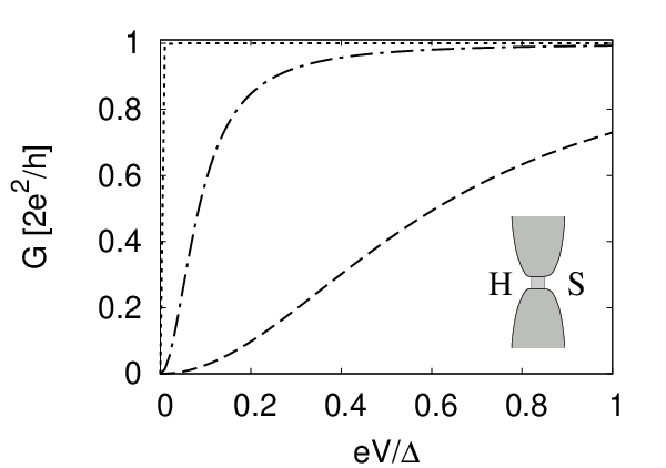
Unlike the quasiclassical approach, the scattering approach can also deal with systems in which the number of orbital modes is small. The simplest way to illustrate this is to consider the contribution of one orbital mode; in this case, the result in Eq. (15) and the corresponding term in Eq. (16) describe a single mode ballistic ferromagnetic quantum point contact between the half-metal and the superconductor. In Fig. 3 we show the differential conductance of such an HS quantum point contact for a few representative values of the ferromagnet parameters $\rho$ and $\theta$. Both aforementioned features are clearly seen: the conductance decreases as $\sin^{2}\theta$ and $\sin^{2}\rho$ decreases, and it vanishes at the Fermi energy.

If the spacer layer between the half-metallic reservoir and the superconductor is not a ferromagnet, but a half metal, transmission through the minority channel is via evanescent modes, not propagating waves. The scattering matrix of the spacer layer, which was given by Eq. (13) for the case of a ferromagnetic spacer, now reads

where

The (mode-dependent) phase shift $\nu_{\downarrow}$ and transmission coefficient $\tau$ for minority electrons are functions of the wavefunction decay rate $q$ and effective mass $m_{\downarrow}$ of the evanescent minority electron wavefunctions, the velocity $v$ of the majority electrons, and the thickness $d$ of the half-metallic spacer layer. If $qd\gg 1$, the minority electron phase shift $\nu_{\downarrow}$ becomes independent of the layer thickness $d$,

whereas the transmission coefficient $\tau\propto e^{-2qd}$ and $\nu_{\uparrow}=m_{\uparrow}vd/\hbar$, where $m_{\uparrow}$ is the effective mass of majority electrons. [The phase shift $\beta$ is the reflection phase for minority electron reflection off a half-infinite half metal, see Eq. (14) above.]

With the definitions $\rho=\nu_{\uparrow}-\nu_{\downarrow}$ and $\eta=\nu_{\uparrow}+\nu_{\downarrow}$, we then find that the conductance of an HS junction with a half-metallic spacer is

where we abbreviated

and restored the summation over the orbital modes $\mu$. For $\tau_{\mu}$ close to unity, this expression simplifies to the Andreev conductance for an HS junction with a ferromagnetic spacer, Eq. (16) above. For small energies one may neglect the terms proportional to $\varepsilon^{2}$ and $\varepsilon^{4}$ in the denominator, and we find that $G\propto\varepsilon^{2}\tau$. Since the transmission coefficients $\tau_{\mu}$ are exponentially small if $q_{\mu}d\gg 1$, the conductance is dominated by the transverse mode $\mu$ with the lowest $q_{\mu}$.

Similar to the case of ideal transmission, there is a special set of parameters at which the conductance becomes large, independent of transmission. This occurs when the coefficient $B_{0}=0$ in Eq. (20), so that the denominator in that equation vanishes at $\varepsilon=0$. The condition $B_{0}=0$ translates to

Solutions of Eq. (21) satisfy the relation $\sin^{2}\rho_{\mu}\sin^{2}\theta=\tau_{\mu}$, which generalizes the condition for resonance found for a ferromagnetic spacer layer (corresponding to $\tau_{\mu}=1$). Since $\nu_{\downarrow\mu}=(\eta_{\mu}-\rho_{\mu})/2$ is a material property if $q_{\mu}d\gg 1$, see Eq. (19) above, $\rho_{\mu}$ and $\eta_{\mu}$ are not independent in that limit. For a specific half metallic material and in the limiting case $q_{\mu}d\gg 1$, the relevant solution of Eq. (21) then becomes $(\rho_{\mu}+\eta_{\mu})/2=\nu_{\uparrow\mu}=\pi/2\mod\pi$ and $\theta\to\pi$. Since $\nu_{\uparrow\mu}$ is a function of the thickness $d$ of the spacer layer, not a material property, this condition can always be satisfied for special values of $d$. If a mode satisfies the conditions (21), its contribution to the conductance is

At zero energy, one finds perfect Andreev reflection irrespective of $\tau_{\mu}$. As before, the contribution of a single orbital mode in Eqs. (20), (22) describes the differential conductance of a single mode quantum point contact with a misaligned half metallic surface layer at the constriction, the analogue of the setup sketched in Fig. 3.

As the next application of the scattering method, we consider a “chaotic HS junction”, which consists of a half-metallic contact, a chaotic quantum dot, a ferromagnetic contact, and a superconductor, all connected in series, see Fig. 4. To illustrate the strengths of the scattering matrix approach, we focus on a situation that is intractable with quasiclassical methods: we restrict our discussion to the case that both contacts have one orbital mode only.

For definiteness, we take the quantum dot to be half metallic, with the same polarization direction as the half-metallic contact. Two alternative scenarios, a normal-metal quantum dot and a ferromagnetic quantum dot with a magnetization direction parallel to that of the half-metallic contact, will be addressed at the end of this section. In all cases we assume that the typical electron path length before exiting from the dot through one of the contacts is short compared to the superconducting coherence length.

The calculation proceeds similar to that of the ballistic junction shown above. For the chaotic HS junction with a half-metallic quantum dot, we replace the scattering matrix $S_{H}$ of Eq. (14) by

where $0\leq\tau\leq 1$ is the transmission coefficient of the quantum dot and $\xi$ and $\chi$ are scattering phases for reflection off the quantum dot. As before, $\beta$ is the phase shift minority electrons acquire when they are reflected off the half metal. The special case $\tau=1$ simplifies to the ballistic HS point contact we considered previously. For general $\tau$, one finds

where

For the special point $\sin^{2}\theta=\sin^{2}\rho=1$ one has $G(0)=2e^{2}/h$, independent of $\tau$ and the scattering phases $\beta$, $\chi$, and $\xi$. The origin of this remarkable result is that, for $\sin^{2}\theta=\sin^{2}\rho=1$, the ferromagnet-superconductor interface not only provides perfect Andreev reflection between spin-up electrons and spin-up holes, but, moreover, after two subsequent Andreev reflections the net phase shift is $-\alpha^{2}=1$ at the Fermi energy. Hence, combining the interface reflection matrix (15) with the scattering matrix of the quantum dot, the conductance at vanishing voltage is found to be

independent of the dot’s transmission coefficient $\tau$. This is to be contrasted to the corresponding formula formula[23]

for the linear response conductance (per spin) of a superconductor in contact with a single mode quantum dot through a normal-metal contact (and without magnetic a field). The difference arises from the fact that, in the latter case, the phase shift upon two Andreev reflections is $\alpha^{2}=-1$ at the Fermi energy.

For a chaotic quantum dot, the transmission coefficient $\tau$ and the scattering phases $0<\xi,\chi<4\pi$ are random quantities with the statistical distribution[18]

As is standard in the statistical approach to quantum transport, the statistical ensemble is obtained by means of small variations of the dot’s shape or of the Fermi energy. In an experiment, both types of variations can be achieved by changing the voltage of nearby metal gates. With the help of the distribution (28) we can calculate the average Andreev conductance $\langle G\rangle$ for an ensemble of quantum dots. The phase shift $\rho$, the angle $\theta$ and the reflection phase $\beta$ are not averaged over, since they are properties of the ferromagnetic contact and the half metal interface, not of the chaotic quantum dot. The average can be performed analytically in the special case $\sin^{2}\rho=\sin^{2}\theta=1$, for which we find

with

where

At the Fermi level $\langle G\rangle=2e^{2}/h$, in agreement with the discussion following Eq. (25). For general values of $\theta$ and $\rho$ no closed-form expression for $\langle G\rangle$ could be obtained. The result of a numerical evaluation of the ensemble average $\langle G(\varepsilon)\rangle$ is shown in Fig. 5 for a few representative values of $\theta$ and $\rho$. For generic $\theta$ and $\rho$, the ensemble-averaged conductance vanishes at the Fermi level $\varepsilon=0$. The quadratic dependence $G\sim\varepsilon^{2}$ for $\varepsilon\rightarrow 0$ changes to a linear increase for relatively small voltages. The conductance reaches a maximum at a voltage $eV$ below the superconducting gap $\Delta$ for $\theta$, $\rho$ sufficiently away from $\sin\theta=0$, $\sin\rho=0$. With $\theta$, $\rho$ approaching $\sin\theta=0$, $\sin\rho=0$, the position of the maximum moves towards the superconducting gap $\Delta$. For $\theta$, $\rho$ close to $\sin\theta=0$, $\sin\rho=0$, the conductance is an increasing function of the voltage in the full subgap regime.

For the case of a normal-metal quantum dot, the conductance $G(\varepsilon)$ is given by Eq. (24), but with the replacement $\beta-\xi\to\arctan[\tau\sin(\beta+\chi)/((2-\tau)\cos(\beta+\chi)+2(1-\tau)^{1/2})]$. For the case of a ferromagnetic quantum dot with a magnetization direction along that of the polarization of the half-metallic contact, $G(\varepsilon)$ is given by Eq. (24), but with $\beta-\xi$ replaced by a phase shift $\beta^{\prime}$ that is statistically independent of $\chi$, $\xi$, and $\tau$. In both cases, the qualitative dependence of $\langle G\rangle$ on the parameters $\varepsilon$, $\theta$, and $\rho$ is the same as in the case of a half-metallic quantum dot discussed above.

For the ballistic SHS junction different orbital modes are not mixed, so that the scattering problem is effectively one-dimensional. As before, we denote the difference of the (mode-dependent) phase shifts of majority and minority electrons transmitted through F by $\rho$, see Eq. (13); The corresponding quantity for F’ is denoted by $\rho^{\prime}$. We suppress the mode index $\mu$, except in the final expressions. For the calculation of the supercurrent, it is necessary that phase shifts accumulated inside the half metal are included into the determinant in Eq. (3). For an orbital mode $\mu$ these phase shifts depend on the length $L$ of the half-metallic segment and on the longitudinal component $k_{\mu}(\varepsilon)=k_{\mu}(0)+\varepsilon/(\hbar v_{\mu})$ of the wave vector for that mode, where $v_{\nu}$ is the group velocity of the mode at $k_{\mu}(0)$. In order to include this into Eq. (3) we take the scattering matrix ${\cal R}^{\prime}$ to include the scattering phase shifts accumulated inside the half metal,

where $\tilde{\cal R}^{\prime}$ is the reflection matrix for the S’H junction without the scattering phases from the half metal. This matrix is given in Eq. (15) of the previous section, but with $\theta$, $\psi$, $\phi$, and $\rho$ replaced by $\theta^{\prime}$, $\psi^{\prime}$, $\phi^{\prime}$, and $\rho^{\prime}$, respectively.

Since there is a probability of normal reflection at each end of the SHS junction, for a given orbital mode, the contribution to the supercurrent contains terms that oscillate with the length $L$ of the junction. For the total supercurrent, obtained by summing the contributions from different orbital modes, however, this results only in a small correction, provided that $k_{\mu}(0)L\gg 1$, since in this case, the sum of the oscillating contributions averages out. Below, we calculate the non-oscillating contribution to the Josephson current for a given orbital mode, and restrict our discussion to the limiting cases of a “short junction” ($L\ll\xi_{S}$) and a “long junction” ($L\gg\xi_{S}$). (In both cases, we assume that the ferromagnetic spacer layers are thin in comparison to the superconducting coherence length $\xi_{S}$. The same assumption was made in the previous section.)

For a short junction, one may neglect the energy-dependence of the wavenumber $k_{\mu}(\varepsilon)$ in the half metal. A closed-form expression valid for arbitrary temperatures could be obtained for the special case $\sin^{2}\theta=\sin^{2}\theta^{\prime}=1$ for a mode $\mu$ with $\sin^{2}\rho_{\mu}=\sin^{2}\rho^{\prime}_{\mu}=1$ only. The contribution $I_{\mu}$ to the supercurrent of such a mode is

where $s_{\mu}$ is defined through the relation

The $\pi$ shift in the current-phase relationship associated with $s_{\mu}$ originates in the properties of the interface reflection matrix (15): for this matrix, the transformation $\rho\rightarrow\rho+\pi$ is equivalent to $\phi\rightarrow\phi+\pi$.

In the limit of high temperatures $k_{B}T\gg\Delta$, one can find a closed-form expression for arbitrary values of $\theta$, $\theta^{\prime}$, $\rho$, and $\rho^{\prime}$. Upon summation over all orbital modes, one has

Note that although the angles $\rho_{\mu}$, $\rho^{\prime}_{\mu}$ are mode dependent, for sufficiently thin spacer layers the mode dependence is weak enough that all modes contribute to the total Josephson current with the same sign. The supercurrent is reduced once the thickness of the spacer layers is large enough that $\rho_{\mu}$, $\rho^{\prime}_{\mu}\gg 1$.

A numerical evaluation of the contributions to the zero-temperature supercurrent is shown in Fig. 6 for a few choices of the angles $\theta$, $\theta^{\prime}$, $\rho$, and $\rho^{\prime}$. Although the discontinuity at $\tilde{\phi}=s\pi$ is smeared for generic values of the phase angles, the order of magnitude of the supercurrent is the same as at the special point $\sin^{2}\theta=\sin^{2}\theta^{\prime}=\sin^{2}\rho=\sin^{2}\rho^{\prime}=1$. This is in contrast to the Fermi-level conductance of an HS junction, which was zero for generic phase angles and finite at the special point. As discussed above, the reason why the supercurrent has a different behavior is that it is not a Fermi-level property but, instead, depends on the entire excitation spectrum. For energies far away from the Fermi level, the Andreev conductance is not qualitatively different at the special point and elsewhere, see Fig. 3.

For a long SHS junction (but still with ferromagnetic spacer layers that are much thinner than $\xi_{S}$), again a compact expression at arbitrary temperatures could be obtained for the special case $\sin^{2}\theta=\sin^{2}\theta^{\prime}=1$, for the contribution $I_{\mu}$ of a mode $\mu$ with $\sin^{2}\rho_{\mu}=\sin^{2}\rho^{\prime}_{\mu}=1$ only. In this case one finds

where $s_{\mu}$ was defined in Eq. (36). At zero temperature the summation can be replaced by an integration and one has

In the limit of high temperatures, $T\gg\hbar v_{\mu}/L$, only the term with $n=0$ contributes, so that

The special point $\sin^{2}\theta=\sin^{2}\theta^{\prime}=\sin^{2}\rho=\sin^{2}\rho^{\prime}=1$ is singular, however, and the supercurrent contributions have a qualitatively different dependence on temperature for generic $\theta$, $\theta^{\prime}$, $\rho$, and $\rho^{\prime}$. In the high-temperature regime $\hbar v_{\mu}/L\ll k_{B}T\ll\Delta$, one finds

This result is a factor $\sim(k_{B}T/\Delta)^{2}\ll 1$ smaller (per orbital mode) than the contribution for the special choice of the angles $\theta$, $\theta^{\prime}$, $\rho$, and $\rho^{\prime}$ in Eq. (40). Whereas the supercurrent of a short Josephson junction depends on the full subgap excitation spectrum of the junction,[24] the supercurrent in the long junction limit is determined by the junction’s excitation spectrum up to the Thouless energy $\hbar v_{F}/L$ only.[22] In this range of the spectrum, the absence of Andreev reflection at the Fermi energy still strongly affects the magnitude of the supercurrent. For temperatures below the Thouless energy $\hbar v_{F}/L$ the suppression factor with which $I_{\mu}$ is reduced in comparison to the special case of Eq. (38) saturates around $(\hbar v_{F}/L\Delta)^{2}$. No closed-form expressions for $I_{\mu}$ at arbitrary temperatures could be obtained. Figure 7, shows $I_{\mu}$ versus $\tilde{\phi}$ at zero temperature, for two choices of the parameters $\theta$, $\theta^{\prime}$, $\rho$, and $\rho^{\prime}$.

For a chaotic SHS junction, we include the quantum dot into ${\cal R}$, and take ${\cal R}^{\prime}=\tilde{\cal R}^{\prime}$ to be the scattering matrix of a junction without quantum dot, see Fig. 8. For the chaotic SHS junction we only consider the limit that the superconducting coherence length is much longer that the typical electron path length in the dot before exiting through one of the contacts.

In the special case $\sin^{2}\theta=\sin^{2}\theta^{\prime}=\sin^{2}\rho=\sin^{2}\rho^{\prime}=1$ the expression for the supercurrent is the same as for a ballistic SHS junction, but with the replacement $\Delta\to\Delta\tau^{1/2}$, where $\tau$ is the transmission coefficient of the quantum dot. Since $\langle\tau^{1/2}\rangle=1/2$, at zero temperature, the ensemble-averaged supercurrent is

where $s$ was defined below Eq. (35). No closed-form expressions could be obtained for generic values of $\theta$, $\theta^{\prime}$, $\rho$, and $\rho^{\prime}$. A numerical evaluation of the ensemble-averaged supercurrent is shown in Fig. 9. For phase angles close to the special case discussed above, the supercurrent in a short chaotic SHS junction follows Eq. (42), except near the discontinuity $\tilde{\phi}=s\pi$, which is smoothed out away from the special point $\sin^{2}\theta=\sin^{2}\theta^{\prime}=\sin^{2}\rho=\sin^{2}\rho^{\prime}=1$. For phase angles not close to the special point, the $\tilde{\phi}$-dependence of the ensemble-averaged supercurrent is nearly sinusoidal, confirming the general observations made in the beginning of this section.

References

- [1] R. S. Keizer, S. T. Goennenwein, T. M. Klapwijk, G. Miao, G. Xiao, and A. Gupta, Nature 439, 825 (2006).
- [2] R. A. de Groot, F. M. Mueller, P. G. van Engen, and K. H. J. Buschow, Phys. Rev. Lett. 50, 2024 (1983).
- [3] W. Pickett and J. Moodera, Physics Today 54, (5) 39 (2001).
- [4] J. Coey and M. Venkatesan, J. Appl. Phys. 91, 8345 (2002).
- [5] F. S. Bergeret, A. F. Volkov, and K. B. Efetov, Phys. Rev. Lett. 86, 4096 (2001a).
- [6] A. Kadigrobov, R. I. Shekhter, and M. Jonson, Europhys. Lett. 54, 394 (2001).
- [7] F. S. Bergeret, A. F. Volkov, and K. B. Efetov, Phys. Rev. B 64, 134506 (2001b).
- [8] M. Eschrig, J. Kopu, J. Cuevas, and G. Schön, Phys. Rev. Lett. 90, 137003 (2003).
- [9] F. S. Bergeret, A. F. Volkov, and K. B. Efetov, Rev. Mod. Phys. 77, 1321 (2005).
- [10] V. Braude and Y. V. Nazarov, Phys. Rev. Lett. 98, 077003 (2007).
- [11] M. Eschrig, T. Löfwander, T. Champel, J. Cuevas, J. Kopu, and G. Schön, J. Low Temp. Phys. 147, 457 (2007).
- [12] Y. Asano, Y. Tanaka, and A. A. Golubov, Phys. Rev. Lett. 98, 107002 (2007).
- [13] Y. Asano, Y. Sawa, Y. Tanaka, and A. A. Golubov, Phys. Rev. B 76, 224525 (2007).
- [14] M. Eschrig and T. Löfwander, Nature Physics 4, 138 (2008).
- [15] A. V. Galaktionov, M. S. Kalenkov, and A. D. Zaikin, Phys. Rev. B 77, 094520 (2008).
- [16] G. Eilenberger, Z. Phys. 214, 195 (1968).
- [17] A. I. Larkin and Y. N. Ovchinnikov, Sov. Phys. JETP 28, 1200 (1969).
- [18] C. W. J. Beenakker, Rev. Mod. Phys. 69, 731 (1997).
- [19] J. Yi-Qun, N. Zhi-Ping, F. Cui-Di, and X. Ding-Yu, Chin. Phys. Lett. 25, 691 (2008).
- [20] G. E. Blonder, M. Tinkham, and T. M. Klapwijk, Phys. Rev. B 25, 4515 (1982).
- [21] Y. Takane and H. Ebisawa, J. Phys. Soc. Jpn. 61, 1685 (1992).
- [22] P. W. Brouwer and C. W. J. Beenakker, Chaos, Solitons and Fractals 8, 1249 (1997).
- [23] C. W. J. Beenakker, Phys. Rev. B 46, 12841 (1992a).
- [24] C. W. J. Beenakker, in: Transport phenomena in Mesoscopic Systems, edited by H. Fukuyama and T. Ando (Springer, Berlin) p. 235 (1992b), arXiv:cond-mat/0406127.
- [25] C. Ishii, Progress of Theoretical Physics 44, 1525 (1970).
- [26] R. M. Potok, J. A. Folk, C. M. Marcus, and V. Umansky, Phys. Rev. Lett. 89, 266602 (2002).