Enhancement effects in exclusive $\pi\pi$ and $\rho\pi$ production in $\gamma^{\ast}\gamma$ scattering

Collisions of a real photon and a highly virtual photon are an useful tool for studying fundamental aspects of QCD. Inside this class of processes, the exclusive meson pair production in $\gamma^{\ast}\gamma$ scattering has been analyzed in Ref. [1] introducing of a new kind of distribution amplitudes, called Transition Distribution Amplitude (TDA). At small momentum transfer $t$ and in the kinematical regime where the photon is highly virtual, a separation between the perturbative and the nonperturbative regimes is assumed to be valid. Through the factorization theorems the amplitude for such reactions can be written as a convolution of a hard part $M_{h}$, the meson distribution amplitude $\phi_{M}$ and a soft part, the TDA, describing the photon-pion transition, as is shown in Fig. 1. Lacking a complete fundamental understanding of the color dynamics, we are compelled to use models for predictions. Cross section estimates for the processes

have been proposed in Ref. [2] using for the TDA a $t$-independent double distributions, in a first approach, and, in a second, the $t$-dependent results of Ref. [3].

The process $\gamma^{\ast}\gamma\rightarrow\pi\pi$ is particularly interesting because different kinematical regimes lead to different mechanisms, which implies a description of the process through either the pion Generalized Distribution Amplitudes or the pion-photon TDAs [4]. Therefore, it is of interest to deepen our understanding of the description of this process. Recently the pion-photon TDAs have been calculated in, respectively, the Spectral Quark Model (SQM) [5], the Nambu - Jona-Lasinio model with Pauli-Villars regularization procedure (NJL) [6] and a nonlocal chiral quark model [7]. A comparison of the results obtained in these three models is given in Ref. [8] concluding that there is clear agreement between the different studies of the pion-photon TDAs, allowing us to analyze the result of a single model, e.g. the NJL model. Our choice is based on the fact that the NJL model [9] is the most realistic model for the pion based on a local quantum field theory built with quarks. It gives a right description of the low energy pion physics. It has been applied to the study of pion parton distribution (PD) [10] and pion generalized parton distribution (GPD) [11]. In the chiral limit, its quark valence distribution is as simple as $q(x)=\theta\left(x\right)~\theta(1-x)$. Once evolution is taken into account, good agreement is reached between the calculated PDF and the experimental one [10]. More elaborated studies of pion PD have been done in the Instanton Liquid Model [12] and lattice calculation based models [13] using nonlocal Lagrangians [14], which confirm that the result obtained in the NJL model for the PD is a good approximation. The QCD evolution of the pion GPD calculated in the NJL model has been also studied in [15].

Before defining the TDAs, we introduce the light-cone coordinates $v^{\pm}=\left(v^{0}\pm v^{3}\right)/\sqrt{2}$ and the transverse components $v^{\bot}=\left(v^{1},v^{2}\right)$ for any four-vector $v^{\mu}$. We define $P=\left(p_{\pi}+p_{\gamma}\right)/2$ and we introduce the light-front vectors $\bar{p}^{\mu}=P^{+}\left(1,0,0,1\right)/\sqrt{2}$ and $n^{\mu}=\left(1,0,0,-1\right)/\left(\sqrt{2}P^{+}\right).$ The momentum transfer is $\Delta=p_{\pi}-p_{\gamma},$ therefore $P^{2}=m_{\pi}^{2}/2-t/4$ and $t=\Delta^{2}$. The skewness variable describes the loss of plus momentum of the incident photon, i.e. $\xi=\left(p_{\gamma}-p_{\pi}\right)^{+}/2P^{+},$ and its value ranges between $-1<\xi<-t/\left(2m_{\pi}^{2}-t\right)$. With these conventions, the vector and axial TDA are defined by

where the pion decay constant is $f_{\pi}=92.4.$ MeV, $\epsilon\left(\xi\right)$ is equal to $1$ for $\xi>0$ and to $-1$ for $\xi<0$ and $\phi_{\pi}(x)$ is the pion DA. Here we have modified the definition given in Refs. [1, 2] in order to introduce the pion pole contribution [3, 6] in Eq. (3). This equation deserves some comments. The pion pole term in (3) describes a point-like pion propagator multiplied by the distribution amplitude (DA) of an on-shell pion. It contributes to the axial current through a different momentum structure and must be subtracted in order to obtain de axial TDA. We emphasize that it is a model independent definition, because we have define the numerator of the pion pole term as the residue at the pole $t=m_{\pi}^{2}$. With this definition, all the structure dependence related to the outgoing $\pi^{\pm}$ is included in $A\left(x,\xi,t\right)$. Moreover, the pion pole contribution can be estimated in a phenomenological way, as we will see later on. With these definitions we recover the sum rules

with the standard definitions for the form factors $F_{V,A}$ appearing in the $\pi^{\pm}\rightarrow\ell^{\pm}\nu\gamma$ decay [16]. Notice that the on-shell pion DA obeys the normalization condition $\int_{0}^{1}dx\,\phi_{\pi}(x)=1$.

The $\gamma^{\ast}\gamma\rightarrow M^{+}\pi^{-}$ process, with $M^{+}=\rho_{L}^{+}$ or $\pi^{+},$ is a subprocess of the $e\left(p_{e}\right)+\gamma\left(p_{\gamma}\right)\rightarrow e\left(p_{e}^{\prime}\right)+M^{+}\left(p_{M}\right)+\pi^{-}\left(p_{\pi}\right)$ process. We follow all the definitions of the kinematics given in the section III.A and Fig. 3 of Ref. [2], with the exception that our $n^{\mu}$ vector is twice the $n^{\mu}$ vector used in [2] (i.e. $n.p=1$ with our definitions). In particular, for massless pions, we have

where $\Delta_{T}=(0,\vec{\Delta}^{\perp},0)$ and therefore $\Delta_{T}^{2}=-\vec{\Delta}^{\perp 2}$. Notice that $\vec{\Delta}^{\perp 2}=(-t)(1-\xi)/(1+\xi)$, with $t<0$. The longitudinal polarization of the incoming virtual photon is $\varepsilon_{L}=\left(2\xi\bar{p}/Q+Qn/(4\xi)\right)$. The real photon polarization is defined by the condition $\varepsilon^{-}=0$ together with the gauge condition $\varepsilon^{+}=0$.

The differential cross section is given by¹¹ 1 A factor $1/4$ is missing in Eq. (23) of Ref. [2]. This typo does not affect to the numerical results reported in that Reference [17]. [2]

with

where $z$ is the light-cone momentum fraction carried by the quark entering the meson $M^{+}$ and $f_{\rho}=0.216\operatorname{GeV}$ and $Q_{q}$ is the electric charge of the quark $q$. The last term on the r.h.s. of Eq. (9) is the pion pole contribution to the amplitude coming from the second term of Eq. (3).

We proceed now to evaluate these integrals. The meson DA is chosen to be the usual asymptotic normalized meson DA, i.e. $\phi_{M}(z)=6z(1-z)$, which cancels the $z$-dependence of the hard amplitude. For the nonperturbative part of the process we use the TDAs evaluated in the NJL model. This approach is based on the determination of the pion as a bound state through the Bethe-Salpeter equation. This guarantees that all invariances of the problem are preserved. As a consequence, the obtained TDAs explicitly verify the sum rules, the polynomiality condition, the isospin relations and have the correct support in $x$ [6].

In Ref. [6] the $\pi^{+}\rightarrow\gamma$ TDAs were calculated, which are connected to the $\gamma\rightarrow\pi^{-}$ TDAs through $CPT$ symmetry [8]

In Figs. 2 and 3 are shown the vector and axial $\gamma\to\pi^{-}$ TDAs for $t=-0.5$ for different $\xi$ values. From Eq. (7) it can be observed that $\xi\geq Q^{2}/\left(2s_{e\gamma}-Q^{2}\right)$. In other words, there is a (positive) lower limit on the value of $\xi$. It is indeed a particularly interesting restriction because the value of $\xi$ defines the shape of the TDAs. In particular, the shape of the axial TDA radically changes according to the sign of the skewness variable; $A(x,\xi,t)$ has, at $x=\pm\xi$, its maximum values for $\xi>0$ (see Fig. 3) while it has its minimum values for $\xi<0$ [8]. However the vector TDA has its maximum and minimum values at $x=\pm\xi$ (see Fig. 2) independently of the sign of the skewness variable. On the other hand, the magnitude of the distributions is controlled by the $t$-dependence. This can be easily understood because the TDAs, that must satisfy the sum rules Eq. (4), are expected to decrease at least as $t^{-1}.$

In order to numerically estimate the cross sections, we need to fix the strong coupling constant. In Ref. [18] is mentioned that a large value of $\alpha_{s}$ ($\alpha_{s}\simeq 1$) is indicated in the case of an asymptotic DA. Using this value for $\alpha_{s}$ we have evaluated the cross section for $\rho$ production. In Fig. 4 we plot this cross section as a function of $\xi$. As we observe, the cross section is largely dominated by the imaginary part of the integral of Eq. (8). The $t$-dependence of the cross section comes from both the overall $\left(-t\right)$ factor present in Eq. (7) and the $t$ dependence of the Vector TDA. Therefore, we expect a decreasing as $t^{-1}$ for large $t$ values. Comparing with the previous results in Ref. [2], we observe that our predictions are higher by a factor 2 or 3.

The $\pi$ production is described through Eq. (9). Here we have a pion pole term which becomes proportional to the electromagnetic pion form factor (FF)

If we use the asymptotic form of the pion DA, i.e. $\phi_{\pi}\left(z\right)$ with $z=\left(x+\xi\right)/2\xi,$ in Eq. (9) we obtain the Brodsky-Lepage pion FF [19]

The cross section for pion production at $Q^{2}=4$ GeV² as a function of $\xi$ is given in Fig. 5(left). This cross section is dominated by the pion pole contribution which is determined by the Brodsky-Lepage pion FF. Alternatively, if the pion FF is experimentally known, we can infer phenomenologically this contribution. And hence the axial TDA could be extracted from the interference term. From Ref. [20] we know that the pion FF at $Q^{2}=2.45\operatorname{GeV}^{2}$ is $0.167\pm 0.010$. In Fig. 5(right) we depict, for each contribution, the prediction using the interval defined by the experimental value of the FF (filled areas), including also the theoretical prediction using the Brodsky-Lepage pion FF (lines).

The $t$-dependence of the cross section for pion production includes a strong dependence on $t$ coming from the pion pole. Neglecting the pion mass in (9), we observe that the pion pole contribution to $\mathcal{I}_{\pi}$ is proportional to $t^{-1}.$ Therefore, the cross section grows as $t^{-1}$ for small $t$ values. For large $t$ values we expect, as in the $\rho$ production case, a decreasing as $t^{-1}.$

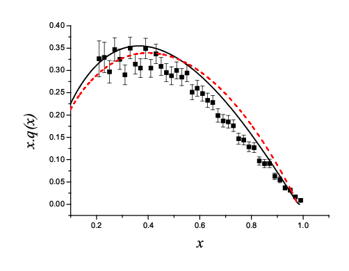
We have also studied the effect of the QCD evolution on our estimates, using for this purpose the code of Freund and McDermott [21]. One needs to fix the value of $Q_{0}$ for which the quark distributions obtained in the NJL model are considered to be a good approximation of the QCD quark distributions. Knowing that the momentum fraction of each valence quark at $Q=2$ GeV is $0.23$ [22], we fix the initial point of the evolution in such a way that the evolution of the second moment of the pion parton distribution reproduces this result. This condition is fulfilled at a rather low value, i.e. $Q_{0}=0.29$ GeV, when the LO evolution is used. Going to the NLO changes this value to $Q_{0}=0.43$ GeV. However, in the latter case, the resulting PD is basically unaffected by the change in $Q$. The effect of the NLO evolution is compensated in the LO evolution going to a lower value of $Q_{0}$, a result that has already been noticed in proton parton distributions [23]. In order to illustrate the latter statement, we have depicted both the evolved pion PD for the LO and the NLO in Fig. 6. Turning our attention to the vector TDA evolved at LO (Fig. 2), we observe that the value of $V\left(x,\xi,t\right)$ at $x=\pm\xi$ grows for small values of $\xi$ and decreases for large $\xi$ values in comparison with the TDA at the scale of the model. This implies that the cross section for $\rho$ production, which is largely dominated by the imaginary part, will grow appreciably in the small $\xi$ region. In Fig. 4 we compare the cross section after evolution, calculated only through contribution of the imaginary part of $\mathcal{I}_{\rho},$ with the one obtained before evolution. We observe that this cross section is multiplied by a factor about 5 in the $\xi\sim 0.2$ region.²² 2 The effect of QCD evolution, if calculated also through the contribution of the real part of $\mathcal{I}_{\rho},$ could lead to a change in the cross section of about 15$\%$, what is within the model’s uncertainties. In the case of the axial TDA, the cross section is dominated by the pion FF contribution, therefore the effect of the evolution is expected to be small.

In many papers present in the literature, the r.h.s. of Eq. (3) contains only the $A$ term. In a general case the $A$ term and the pion pole terms have different tensor structures, but we can fix the gauge convention in such a way that these two structures coincide, as we have done in this paper. In that case we can change our definition of the axial TDA

with

The latter expression shows that the pion pole contribution to the axial TDA is closely related to the $D$-term of the Generalized Parton Distributions [25]. Nevertheless, it must be realized that in this case it gives an explicit contribution to the sum rule

In this paper we have looked at the expected cross section for $\pi$-$\pi$ and $\pi$-$\rho$ production in exclusive $\gamma^{\ast}\gamma$ scattering in the forward kinematical region using realistic models for the description of the pion. First we confirm the previous estimates for $\rho$ production, even if our results for the cross section are a factor 2 larger than the one obtained in Ref. [2]. Second, in comparison with this previous evaluation of the cross sections, we have improved in considering the effect of evolution on the vector current. In doing so, an additional factor 5 appears in the small $\xi$ region, leading to a cross section for $\rho$ production of one order of magnitude larger than the previous calculation. We have also improved in including the pion pole term in the tensor decomposition of the axial current. Then an even larger enhancement factor, of about 60 in this case, is found in the cross section for pion production. The interference term becomes a factor 15 larger than the pure TDA contribution, making the axial TDA more accessible experimentally. The interest on TDAs is actually extended to other transitions such as $\gamma^{\ast}N\rightarrow N^{\prime}\pi,$ $\gamma^{\ast}N\rightarrow N^{\prime}\gamma,$ $N\bar{N}\rightarrow\gamma^{\ast}\gamma,$ which are related to $N$-$\pi$ and $N$-$\gamma$ transition distribution amplitudes [26, 27, 28].