Hard loop effective theory of
the (anisotropic) quark gluon plasma
Abstract
The generalization of the hard thermal loop effective theory to anisotropic plasmas is described with a detailed discussion of anisotropic dispersion laws and plasma instabilities. The numerical results obtained in real-time lattice simulations of the hard loop effective theory are reviewed, both for the stationary anisotropic case and for a quark-gluon plasma undergoing boost-invariant expansion.
1 Introduction
1.1 Weakly vs. strongly coupled quark-gluon plasma
The wealth of data harvested at the Relativistic Heavy Ion Collider (RHIC) [1] has led to a shift of paradigm in thinking about the quark-gluon plasma. The strong collectivity that is being observed, in particular in elliptic flow and jet quenching, is widely taken as pointing to a strongly coupled plasma which is qualitatively and quantitatively different from a parton plasma that can be described by perturbative quantum chromodynamics (QCD); for an opposing point of view see however Ref. [2].
In fact, already before the mounting experimental evidence for a strongly coupled quark gluon plasma (sQGP) at RHIC, perturbative QCD at finite temperature was in some difficulty describing lattice data on the thermodynamics of deconfined QCD. Lattice results for the thermodynamic pressure of QCD typically lead to a rather sudden rise of pressure and entropy to about 15-20 % of the Stefan-Boltzmann result for an ultrarelativistic gas of quarks and gluons, at a few times the transition temperature . A straightforward first-order calculation in in fact gives just this ballpark of deviations from the interaction-free result. Higher-order calculations require resummation of collective effects such as Debye screening and have been carried through to order [3, 4, 5], but at face value they show hopelessly poor convergence of perturbation theory at all temperatures of practical interest (in fact up to ridiculously high temperatures ).
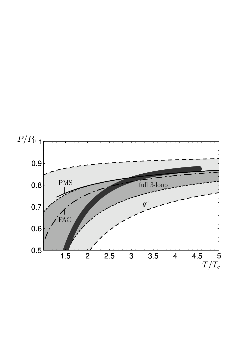
However, it is now understood that the poor convergence properties of thermal perturbation theory beyond first order perturbation theory is at least to a large part signalling the need for more complete resummations of screening phenomena, since similar problems appear already in the rather trivial case of scalar O() models, which can be solved exactly and where the only effect is the generation of a thermal mass [8]. Indeed, already a minimal resummation of the Debye mass beyond strict perturbation theory together with a simple optimizations of the (huge) renormalization scale dependence [7] (see Fig. 1) gives a remarkably good description of the (continuum-extrapolated) lattice results down to about . Fig. 2a shows that a description of the entropy of (pure glue) QCD in terms of hard-thermal-loop (HTL) resummed quasiparticle propagators together with a standard 2-loop running coupling (with renormalization scale varied about the Matsubara scale ) also gives a good description of the thermodynamics above about [9] (see also Ref. [10] and references therein).11 1 HTL quasiparticle models have also been used as phenomenological models down to the phase transition by adding fitting parameters in the running coupling [11, 12, 13], sometimes extended by incorporating quasiparticle damping in a form motivated by HTL perturbation theory [14, 15].
Meanwhile, new techniques have become available that allow the analytical treatment of strongly coupled gauge theories. In particular, supersymmetric Yang-Mills theories (SYM) in the limit of large number of colors and strong ’t Hooft coupling is now often taken as a model for hot QCD. On the basis of the AdS/CFT conjecture [16, 17] one can make predictions for the otherwise inaccessible strong-coupling regime, notably for real-time quantities such as the specific shear viscosity . While at weak coupling [18, 19], the AdS/CFT correspondence gives at large ’t Hooft coupling [20, 21], and such (extremely) low values seem to be indeed required in viscous hydrodynamics models of heavy-ion collisions at RHIC [22]
For SYM at finite temperature, no lattice results for the thermodynamic potential are available that would allow one to test either weak coupling results or the (conjectured) strong coupling results at finite coupling (which does not run because of conformal invariance). However, successive Padé approximants that interpolate between the known weak and strong coupling results give smooth and seemingly robust extrapolations, as shown in Fig. 2b [23]. A comparison of the QCD results for the entropy with those for SYM suggests that the strong-coupling expansion is no longer working well when the deviations from the Stefan-Boltzmann result () are less than some 15%, as is the case for QCD at temperatures above . Such temperatures are expected to be reached in the heavy-ion experiments at the LHC, which may eventually get to probe specific perturbative features of the quark-gluon plasma. But already in the case of RHIC physics, it is clearly mandatory to improve our understanding of both the weak and the strong coupling asymptotics of the quark-gluon plasma, as the truth will most probably be somewhere in between, perhaps quite far from either.


(a) (b)
In some respect, a weakly coupled quark-gluon plasma (wQGP) can be more difficult to describe than a strongly coupled one, in which strong coupling dynamics wipes out any structures from quasiparticle dynamics. In a wQGP, a small coupling leads to a hierarchy of scales, which need to be disentangled by assuming . Of course, for quantitative predictions, extrapolations to have to be considered, but this is no more or less problematic than the equally bold extrapolations theoretician need to do by starting out from infinite (’t Hooft) coupling.
1.2 Scales of wQGP
In thermal equilibrium, the primary scale is the temperature , which determines the mean energy of (“hard”) particles in the plasma. The “soft” scale with is the scale of thermal masses that determine the plasma frequency, below which no propagating modes exist, the Debye screening mass, and the scale of Landau damping. In Feynman diagrams, these effects come from one-loop contributions with the highest power of the loop momentum, cut off by the thermal distribution function, and are therefore called hard thermal loops (HTL). To determine the physics at softer scales, one typically needs to consider the effective HTL theory and its resummed propagators and vertices.
At the scale one encounters in fact a barrier for perturbation theory when the magnetostatic sector is involved, since the latter is characterized by a completely nonperturbative dimensionally reduced Yang-Mills theory, which by itself can be (comparatively easily) handled by lattice methods (the difficult part being the perturbative matching to the four-dimensional theory). Quantities such as the color relaxation or gluon damping rate [24, 25] and also the Debye screening length at next-to-leading order [26] involves logarithms of the coupling, whose coefficient can be calculated perturbatively, but which are nonperturbative beyond the leading log.
The scale is the one characteristic of large-angle scattering and also of the inverse shear viscosity , whose calculation at weak coupling [18, 19] requires resummations beyond, but building upon, hard thermal loops.
When it comes to nonequilibrium physics, it turns out that the parametrically most important phenomena are plasma instabilities [27, 28] that appear already in the collisionless limit, on the level of the HTL masses (and only those of gauge bosons [29]). As pointed out by Arnold et al. [30], this leads for instance to the necessity of a complete revision (still to be worked out) for systematic perturbative scenarios of thermalization [31]. Intriguingly, plasma instabilities may also be responsible for anomalous contributions [32] to the inverse shear viscosity whose standard weak coupling result appears much too small (which is one of the key arguments in favor of sQGP).
2 Hard thermal and hard anisotropic loops
2.1 Hard (thermal) loop effective theory
The effective HTL theory of QCD [33, 34] is given by the collection of all one-loop diagrams which are proportional to , assuming that all external momenta are soft and therefore negligible compared to . For external momenta , the HTL self energy and vertex diagrams are parametrically of the same order as the corresponding tree-level quantities and therefore need to be resummed completely. A remarkably compact form of the HTL effective action can be written down formally [35], which for gluons reads
| (1) |
Here is the Debye mass in the HTL approximation, a normalized average over the directions in with , and the covariant derivative in the adjoint representation. In the non-Abelian case, this leads to an effective action which is nonlocal and nonpolynomial, containing an infinity of vertex functions. The reason for nonlocality is that, in contrast to other examples of an effective field theory, one is integrating out stable real particles rather than virtual ones. Albeit elegant in form, the effective action (1) is not well-defined as it stands, because it still requires boundary conditions to be taken into account after the extraction of self energy and vertex diagrams.
Alternatively, the HTL effective theory can be derived from the effective field equation
| (2) |
where is a linearized perturbation of the color-neutral background (thermal) distribution of color-carrying hard particles , , satisfying gauge covariant Boltzmann-Vlasov equations [36]
| (3) |
HTL vertex functions are then defined as the functional derivatives of the induced current with respect to . In particular, the HTL gauge boson self energy is given by the linear terms in , which in Fourier space and imposing retarded boundary conditions reads
| (4) |
Written as gauge-covariant Boltzmann-Vlasov equations, the HTL effective theory allows us to immediately generalize to nonthermal cases. When the background distribution function is stationary and homogeneous, i.e. only dependent on momentum, one can in fact still write down an effective action similar to (1) [37]. The main difference to the thermal situation is that need no longer be proportional to and thus . Whereas in the thermal (or just isotropic) case, the magnetic term in the Vlasov equation (3) drops out, in the anisotropic case magnetic interactions lead to much more complicated and rich dynamics.
2.2 Isotropic dispersion laws

In the isotropic case, the polarization tensor in (4), which is transverse with respect to the 4-momentum , contains two structure functions corresponding to the two symmetric and transverse tensors , with and plasma rest-frame velocity ,
| (5) | |||
| (6) |
As a consequence, the gauge boson propagator, which in Landau gauge reads
| (7) |
has two branches of poles, corresponding to two different dispersion laws, for spatially transverse polarizations, and for polarizations along .
The two branches of poles are shown in Fig. 3, plotted in over in order to show poles corresponding to propagating modes () and poles corresponding to screening (), which are analytically connected, on the same plot. Propagating modes are seen to exist for , with the transverse mode approaching the mass hyperboloid asymptotically. The poles of branch approach the light-cone exponentially, and in doing so, their residues vanish also exponentially, signifying a purely collective mode. For frequencies below the plasma frequency, , there is screening of both electric and magnetic fields, with screening lengths depending on frequency. In the static limit, mode has inverse screening length , the so-called Debye mass. This corresponds to the screening of (chromo-)electric charges in the medium. By contrast, mode has infinite screening length in the limit of vanishing frequency, corresponding to the absence of (chromo-)magnetostatic screening in the HTL approximation.
2.3 Anisotropic dispersion laws and plasma instabilities
In the anisotropic case, the fact that is symmetric and fixed by transversality would lead to 6 structure functions in general. Assuming that there is just one direction of momentum space anisotropy, (i.e., axisymmetry around the -axis), one can define 4 symmetric tensors for , corresponding to 4 independent structure functions.
Defining spatial tensors
| (8) |
with and decomposing the spatial part of according to
| (9) |
one finds that the gluon propagator in temporal axial gauge reads [38]
| (10) | |||
| (11) |
This propagator contains one branch of poles from , and in general two branches from , except when and thus , in which case there are only two branches in total.

A special important case for an axisymmetric distribution function is given by
| (12) |
with some isotropic (for instance thermal) function . The anisotropy parameter is allowed to take values from to , with corresponding to prolate (cigar-shaped) momentum anisotropy, and corresponding to oblate (squashed) distributions. The polarization tensor in the (anisotropic) hard loop (HL) approximation (4) can then be evaluated in closed form [38]. Changing variables gives
| (13) | |||||
As a simple special case, let us consider structure function for the case that and in the static limit where has the interpretation of magnetostatic screening mass squared. One easily finds
| (14) |
which is plotted in Fig. 4.
For , vanishes, reproducing the result that there is no HTL magnetostatic screening mass. However, for (prolate momentum anisotropy) we obtain a nonvanishing HL magnetostatic screening mass, and for this mass turns out to be imaginary, signalling an instability.

This magnetic instability can be identified with the so-called Weibel instability [40] and is illustrated in Fig. 5. In an extremely oblate momentum distribution, where all hard particles move in planes orthogonal to the -axis, a small seed magnetic field with wave vector in the -direction tends to sort streams of charged particles in a way which leads to an induced current that reinforces the initial field. The induced current and the magnetic field grow exponentially, until the magnetic field is large enough to bend the trajectories of the hard particles significantly, which in an Abelian plasma provides a mechanism for fast isotropization. Of course, in the HL approximation, we can only study the onset of such instabilities, because the backreaction on the background distribution is neglected.
In fact, there are also instabilities when , but to see those we have to consider wave vectors pointing away from the -axis. For small , one finds that in the static limit there are the following poles for real wave vector with ,
| (15) | |||||
| (16) |
Thus, when , there are space-like poles in when , corresponding to electric (Buneman) instabilities [30].

Returning to the case of oblate distribution functions, , and restricting again to (i.e., ), which gives the largest tachyonic mass, let us now consider the dependence on frequency in order to determine the full dispersion laws. With one finds [38]
| (17) | |||||
| (18) | |||||
The resulting poles in and are plotted in Fig. 6 by full and dashed lines, respectively, for the three cases (isotropic), (prolate), and (oblate).
In the prolate case, , we see that there is magnetic screening down to and including the static limit, whereas the electrostatic screening is somewhat diminished (for fixed ). In the oblate case, , the latter is instead enlarged but there is now a pole at zero frequency and positive , which is analytically connected with the dynamical magnetic screening poles at by a line of poles with real and negative . The corresponding imaginary values give the momentum-dependent growth rate of the unstable magnetic modes. These growth rates are shown in more detail in Fig. 7 for various values of .

One can show that in the limit of large , the unstable modes are characterized by , but . Compared to the asymptotic gluon mass one has and .
3 Discretized hard-loop effective theory
In the Abelian case, the above dispersion laws give already a complete overview of the stable and unstable modes to leading order in the HL approximation. In particular, the unstable modes grow exponentially with rate until finally the limit of the HL approximation is reached and backreaction on the hard particle distribution has to be considered. However, with non-Abelian fields, the HL effective theory involves infinitely many vertex functions which become important when unstable modes have grown to amplitudes so large that the two terms in the covariant derivative are comparable, i.e., when . This is still within the HL approximation, since hard particles have momentum and so backreaction on them becomes important only when . It is therefore an important question whether non-Abelian plasma instabilities are able to grow beyond the intrinsically non-Abelian regime , and this question is one that can be answered entirely within the HL approximation.
In order to cope with the nonlocal structure of the HL effective theory, it is useful to introduce an auxiliary field formulation as developed in the HTL case in [41, 42]. Factorizing
| (19) |
one has
| (20) |
and
| (21) |
In the latter equation, only one linear combination of the four fields participates in the dynamical evolution. This extra field is a field on both, configuration space and velocity space, but in terms of this field together with the gauge potential, the dynamical equations are local and polynomial. These equations can therefore be solved by real-time lattice simulations upon discretizing both spacetime and velocity space. The induced current can then be written simply as
| (22) |
by introducing vectors covering the unit sphere. In the HTL case, such a discretization has been studied first in [43], whereas [44] performed lattice simulations involving truncated series of spherical harmonics for that purpose.

The first lattice study of non-Abelian plasma instabilities using discretized hard loops was performed in [45] for modes with . The restriction to modes which are constant with respect to spatial directions perpendicular to leads to the great simplification of a dimensional reduction to 1+1 spacetime dimensions that need to be discretized in addition to the 2-dimensional (compact) velocity space. The results obtained showed complicated nonlinear dynamics when Weibel instabilities enter the intrinsically non-Abelian regime, but except for a brief period of stagnation, it appeared that non-Abelian plasma instabilities continue to grow exponentially also in the late phase of the HL evolution, suggesting that they are essentially as effective for fast isotropization as their Abelian counterparts in conventional plasma physics. Closer inspection reveals that this continued growth is brought about by an effective Abelianization of the non-Abelian modes over extended (but finite) spatial domains.
However, subsequent fully 3+1-dimensional lattice simulations [46, 47] showed that this phenomenon is only true for the modes with exactly . If there are also unstable modes with more general wave vectors, they eventually destroy the local Abelianization and lead to a saturation of the exponential growth, which goes over into a slow linear one (Fig. 9). As Fig. 10 shows, at the level of the individual modes this is accompanied by the build-up of an energy cascade where the energy fed into the soft unstable modes by the Weibel instability is distributed to higher-momentum stable modes through non-Abelian self-interactions [48, 49].


More recent lattice simulations using larger lattices and larger (oblate) anisotropy Ref. [50] found a continued exponential growth of initially small perturbations in the case of very strong momentum anisotropy, at least for small initial field configurations, similar to the behavior of the 1+1-dimensional case. With generic large initial gauge field amplitudes, again a linear growth was observed.
4 Quark-gluon plasma instabilities in Bjorken expansion
In the above treatment of anisotropic plasmas, a space-time independent background distribution was considered with a fixed momentum-space anisotropy. A somewhat more realistic case appropriate for the early stage of a quark-gluon plasma in formation after a collision of large nuclei is given by a distribution of hard massless particles which expands in one spatial dimension (the beam axis) in a boost-invariant manner.
In the latter case it is convenient to switch to comoving spacetime coordinates, proper time and rapidity ,
| (23) |
with metric tensor . Momenta are parametrized by
| (24) |
with . A boost-invariant, transversely isotropic, free-streaming background distribution is then given by
| (25) |
where is the boosted longitudinal momentum. Compared to (12) we now have a proper-time dependent anisotropy parameter
| (26) |
such that there is an increasingly oblate momentum-space anisotropy for . This solves
| (27) |
because . (Note that .)
Clearly, we need to start at some finite in order to avoid a singularity at . But a particle description of the initial stage of a heavy-ion collision can anyway make sense only after some finite time after the collision. In the so-called Color-Glass-Condensate (CGC) framework the earliest time when this is beginning to make sense is provided by the inverse saturation scale . In this framework, the initial hard-gluon density is given by [51]
| (28) |
where is the so-called gluon liberation factor. For definiteness, we shall assume in what follows, and we shall also assume that , i.e., that the momentum distribution is always strongly anisotropic with positive .
With increasing (proper) time, we have an increasing anisotropy with more and more modes becoming unstable, but at the same time the density decreases, which tends to diminish the growth rate. The competition between these effects will of course modify the evolution of non-Abelian plasma instabilities, but, at least in the free-streaming idealization, the HL framework can be generalized to study this case as well.
Since (with index upstairs!) we can again solve the Vlasov equation
| (29) |
by introducing auxiliary fields according to
| (30) |
with satisfying
| (31) |
where we now define
| (32) |
The induced current in the non-Abelian Maxwell equations, which in comoving coordinates now read
| (33) |
is given by
| (34) |
with
| (35) |
In the expanding case, already the effectively Abelian, weak-field behavior is highly nontrivial, leading to complicated integro-differential equations [52], from which one can extract that Weibel instabilities behave asymptotically like
| (36) |
where is the wave number corresponding to the rapidity variable , and
| (37) |
For both and large, this leads to
| (38) |
which can be understood by the large- limit of quoted at the end of Sect. 2.3 together with the fact that the thermal mass scale drops like the square root of hard particle density, which behaves as . Such a behavior was found previously in numerical CGC simulations that include small rapidity fluctuations [53].

In order to also investigate specific non-Abelian dynamics in the HL framework, it is again necessary to discretize space-time, now parametrized by proper-time and rapidity coordinates, and the non-compact velocity/momentum-rapidity space parametrized by and . In fact, because the integrand in (34) is exponentially suppressed at large , only a finite rapidity interval is required in numerical simulations.
Fig. 11 shows the results of a real-time lattice simulation [54] of the expanding HL equations (31) and (34) with small initial seed fields that are constant in transverse space and supplied with an initial spectrum inspired by the CGC scenario [55] and a gluon-liberation factor [56] (which is also close to the recent numerical results of Ref. [57]). Given the findings in stationary anisotropic plasmas, the growth of non-Abelian plasma instabilities in the 1+1-dimensional setting probably gives an upper bound on more generic cases. Considering that for GeV for RHIC and GeV for the LHC and that thus the maximal time in Fig. 11 corresponds to some 20 fm/c for RHIC and 7 fm/c for the LHC, one finds an uncomfortably long delay for the onset of plasma instabilities at least for RHIC. Further studies of more generic initial conditions (including then also strong initial fields) are clearly called for to investigate this situation in more generality.
5 Conclusion
The extension of the HTL effective theory to anisotropic plasmas leads to a (leading-order) theory of non-Abelian plasma instabilities, which in the weak-field limit can be analysed by the study of dispersion laws, but which in the strong-field case requires numerical simulations on real-time lattices. The latter have shown that contrary to initial expectations non-Abelian plasma instabilities tend to saturate in the nonlinear regime where fields are nonperturbatively large, but not yet large enough for immediately modifying the anisotropic background distribution of hard particles. However, a complete isotropization scenario still needs to be worked out. Moreover, when boost-invariant expansion is taken into account, there is an uncomfortably long delay for the onset of growth, which seems too long for the environment provided by RHIC, though not necessarily for the LHC, which may be where wQGP physics eventually comes into its own.
It should be kept in mind that the above studies are based on a truly weakly coupled situation with and it is perhaps not so surprising that at least RHIC physics lies outside of the results obtained by extrapolation to , since this is also the case when perturbative thermodynamic bulk results are extrapolated to below 2–3 . Indeed, numerical simulations which do not separate collective HL physics from other interactions have concluded that fast thermalization through plasma instabilities may be indeed possible, see [58].
Still, it remains a theoretical challenge to understand these issues in the limit where a systematic perturbative analysis should be possible, and, as said, perhaps this turns out to find applications eventually at the higher scales to be probed by the LHC.
On the theoretical side, a systematic treatment of the HL effective theory also offers new conceptual problems, as shown by its application to heavy-ion observables such as energy loss [59] and the momentum broadening of jets [60, 61, 62]. There is clearly more work to be done, both numerically and analytically.
Acknowledgments
I would like to thank the organizers of the 30th Course of the International School on Nuclear Physics in Erice for a wonderful meeting. The work presented here was supported by FWF project no. P19526.
References
- [1] M. J. Tannenbaum, Rept. Prog. Phys. 69 (2006) 2005.
- [2] Z. Xu, C. Greiner, H. Stöcker, J. Phys. G35 (2008) 104016.
- [3] P. Arnold, C.-X. Zhai, Phys. Rev. D50 (1994) 7603.
- [4] E. Braaten, A. Nieto, Phys. Rev. D53 (1996) 3421.
- [5] K. Kajantie, M. Laine, K. Rummukainen, Y. Schröder, Phys. Rev. D67 (2003) 105008.
- [6] G. Boyd, J. Engels, F. Karsch, E. Laermann, C. Legeland, M. Lütgemeier, B. Petersson, Nucl. Phys. B469 (1996) 419.
- [7] J. P. Blaizot, E. Iancu, A. Rebhan, Phys. Rev. D68 (2003) 025011.
- [8] I. T. Drummond, R. R. Horgan, P. V. Landshoff, A. Rebhan, Nucl. Phys. B524 (1998) 579.
- [9] J. P. Blaizot, E. Iancu, A. Rebhan, Phys. Rev. D63 (2001) 065003.
- [10] J. O. Andersen, M. Strickland, Ann. Phys. 317 (2005) 281.
- [11] A. Peshier, B. Kämpfer, O. P. Pavlenko, G. Soff, Phys. Rev. D54 (1996) 2399.
- [12] A. Rebhan, P. Romatschke, Phys. Rev. D68 (2003) 025022.
- [13] R. Schulze, M. Bluhm, B. Kämpfer, Eur. Phys. J. ST 155 (2008) 177.
- [14] A. Peshier, Phys. Rev. D70 (2004) 034016.
- [15] W. Cassing, Nucl. Phys. A795 (2007) 70.
- [16] J. M. Maldacena, Adv. Theor. Math. Phys. 2 (1998) 231.
- [17] O. Aharony, S. S. Gubser, J. M. Maldacena, H. Ooguri, Y. Oz, Phys. Rept. 323 (2000) 183.
- [18] P. Arnold, G. D. Moore, L. G. Yaffe, JHEP 0305 (2003) 051.
- [19] S. C. Huot, S. Jeon, G. D. Moore, Phys. Rev. Lett. 98 (2007) 172303.
- [20] G. Policastro, D. T. Son, A. O. Starinets, Phys. Rev. Lett. 87 (2001) 081601.
- [21] A. Buchel, Nucl. Phys. B803 (2008) 166.
- [22] P. Romatschke, U. Romatschke, Phys. Rev. Lett. 99 (2007) 172301.
- [23] J. P. Blaizot, E. Iancu, U. Kraemmer, A. Rebhan, JHEP 06 (2007) 035.
- [24] R. D. Pisarski, Phys. Rev. D47 (1993) 5589.
- [25] F. Flechsig, A. K. Rebhan, H. Schulz, Phys. Rev. D52 (1995) 2994.
- [26] A. K. Rebhan, Phys. Rev. D48 (1993) 3967.
- [27] S. Mrówczyński, Phys. Lett. B214 (1988) 587; Phys. Lett. B314 (1993) 118.
- [28] Y. E. Pokrovsky, A. V. Selikhov, JETP Lett. 47 (1988) 12.
- [29] B. Schenke, M. Strickland, Phys. Rev. D74 (2006) 065004.
- [30] P. Arnold, J. Lenaghan, G. D. Moore, JHEP 08 (2003) 002.
- [31] R. Baier, A. H. Mueller, D. Schiff, D. T. Son, Phys. Lett. B502 (2001) 51.
- [32] M. Asakawa, S. A. Bass, B. Müller, Phys. Rev. Lett. 96 (2006) 252301.
- [33] J. Frenkel, J. C. Taylor, Nucl. Phys. B334 (1990) 199.
- [34] E. Braaten, R. D. Pisarski, Nucl. Phys. B337 (1990) 569.
- [35] E. Braaten, R. D. Pisarski, Phys. Rev. D45 (1992) 1827.
- [36] J.-P. Blaizot, E. Iancu, Phys. Rept. 359 (2002) 355.
- [37] S. Mrówczyński, A. Rebhan, M. Strickland, Phys. Rev. D70 (2004) 025004.
- [38] P. Romatschke, M. Strickland, Phys. Rev. D68 (2003) 036004; Phys. Rev. D70 (2004) 116006.
- [39] S. Mrówczyński, Acta Phys. Polon. B37 (2006) 427.
- [40] E. S. Weibel, Phys. Rev. Lett. 2 (1959) 83.
- [41] V. P. Nair, Phys. Rev. D48 (1993) 3432.
- [42] J.-P. Blaizot, E. Iancu, Nucl. Phys. B421 (1994) 565.
- [43] A. Rajantie, M. Hindmarsh, Phys. Rev. D60 (1999) 096001.
- [44] D. Bödeker, G. D. Moore, K. Rummukainen, Phys. Rev. D61 (2000) 056003.
- [45] A. Rebhan, P. Romatschke, M. Strickland, Phys. Rev. Lett. 94 (2005) 102303.
- [46] P. Arnold, G. D. Moore, L. G. Yaffe, Phys. Rev. D72 (2005) 054003.
- [47] A. Rebhan, P. Romatschke, M. Strickland, JHEP 0509 (2005) 041.
- [48] P. Arnold, G. D. Moore, Phys. Rev. D73 (2006) 025006.
- [49] P. Arnold, G. D. Moore, Phys. Rev. D73 (2006) 025013.
- [50] D. Bödeker, K. Rummukainen, JHEP 07 (2007) 022.
- [51] R. Baier, A. H. Mueller, D. Schiff, D. T. Son, Phys. Lett. B539 (2002) 46.
- [52] P. Romatschke, A. Rebhan, Phys. Rev. Lett. 97 (2006) 252301.
- [53] P. Romatschke, R. Venugopalan, Phys. Rev. D74 (2006) 045011.
- [54] A. Rebhan, M. Strickland, M. Attems, Phys. Rev. D78 (2008) 045023.
- [55] K. Fukushima, F. Gelis, L. McLerran, Nucl. Phys. A786 (2007) 107.
- [56] Y. V. Kovchegov, Nucl. Phys. A692 (2001) 557.
- [57] T. Lappi, Eur. Phys. J. C55 (2008) 285.
- [58] A. Dumitru, Y. Nara, M. Strickland, Phys. Rev. D75 (2007) 025016.
- [59] P. Romatschke, M. Strickland, Phys. Rev. D69 (2004) 065005; Phys. Rev. D71 (2005) 125008.
- [60] P. Romatschke, Phys. Rev. C75 (2007) 014901.
- [61] R. Baier, Y. Mehtar-Tani, Jet quenching and broadening: the transport coefficient in an anisotropic plasma, arXiv:0806.0954 (2008).
- [62] M. E. Carrington, A. Rebhan, Next-to-leading order static gluon self-energy for anisotropic plasmas, arXiv:0810.4799 (2008).