Relevance of equilibrium in multifragmentation
Abstract
The relevance of equilibrium in a multifragmentation reaction of very central collisions at 35 MeV/nucleon is investigated by using simulations of antisymmetrized molecular dynamics (AMD). Two types of ensembles are compared. One is the reaction ensemble of the states at each reaction time in collision events simulated by AMD, and the other is the equilibrium ensemble prepared by solving the AMD equation of motion for a many-nucleon system confined in a container for a long time. The comparison of the ensembles is performed for the fragment charge distribution and the excitation energies. Our calculations show that there exists an equilibrium ensemble that well reproduces the reaction ensemble at each reaction time for the investigated period fm/. However, there are some other observables that show discrepancies between the reaction and equilibrium ensembles. These may be interpreted as dynamical effects in the reaction. The usual static equilibrium at each instant is not realized since any equilibrium ensemble with the same volume as that of the reaction system cannot reproduce the fragment observables.
pacs
25.70.PqI Introduction
In medium-energy heavy-ion collisions at around the Fermi energy, intermediate-mass fragments as well as a large number of light particles such as nucleons and alpha particles are copiously produced [1, 2, 3, 4, 5]. This phenomenon is called multifragmentation. It is a challenging problem to understand the complex but rich quantum many-body dynamics of multifragmentation. One of the purposes of studying heavy-ion collisions is to explore the properties of nuclear matter [6, 7]. This information is valuable not only for nuclear physics but also for astrophysical interests such as supernova explosions and the structure of neutron stars [8]. The nuclear matter is expected to be compressed in the initial stage of a collision and the created compressed matter then expands afterward. The study of heavy-ion collisions thus offers a possibility to probe the properties of nuclear matter in a wide range of density. Multifragmentation has been considered to occur in the expanding stage and to have some connection to the nuclear liquid-gas phase transition, the existence of which is speculated based on the resemblance between the equation of state of homogeneous nuclear matter and that of a van der Waals system. Intensive research has been carried out to find evidence of this phase transition in experimental data of multifragmentation. In some works it is claimed that indications have been obtained [9, 5, 15, 10, 11, 12, 13, 14]. However, they are not conclusive and much effort is still required.
One of the difficulties is that it is not straightforward to relate the experimental data of heavy-ion collisions with the statistical properties of nuclear matter unless the state variables such as the temperature are well defined in dynamical reactions. The typical reaction time scale of multifragmentation reactions is the order of 100 fm/, which may not be long enough for the system to reach equilibrium compared with the typical time scale of successive two-nucleon collisions (a few tens of fm/). However, there are several reports that support the achievement of equilibrium. An example is the existence of several types of scaling laws that appear in experimental data (e.g. Fisher’s scaling [13] and isoscaling [16, 17]), which may be understood if the system has reached equilibrium. Another example is the reasonable reproduction of the fragment mass (charge) distribution by statistical models for some multifragmentation reactions [19, 20, 21, 18, 22]. However, the achievement of equilibrium in multifragmentation reactions is still a controversial issue. One of the difficulties is that the information obtained directly from experiments is that of the very last stage of the reactions. Even if the system reaches equilibrium, the system undergoes the sequential decay process that distorts the information at the stage of the equilibrium before the fragments are finally detected in experiments. Another difficulty is that even if the equilibrium is relevant to multifragmentation reactions the achievement can be incomplete. Several aspects are expected to reflect the reaction dynamics, such as the pre-equilibrium emissions of light particles, the collective flow, and the expansion of the system [24, 25, 26, 23, 27].
The aim of this paper is to investigate whether the concept of equilibrium is relevant in multifragmentation, and if so, in what sense. We examine the achievement of equilibrium in multifragmentation reactions simulated by antisymmetrized molecular dynamics (AMD) [28, 29, 30]. AMD is a microscopic dynamical model based on the degrees of freedom of interacting nucleons. AMD is a suitable model for this study for the following reasons: It has been shown that various aspects of experimental data are reproduced by applying AMD to nuclear reactions [28, 29, 36, 31, 32, 30, 23, 33, 34, 35]. It has been also argued that the quantum and fermionic statistical properties of nuclear systems are correctly described by AMD if an appropriate quantum branching process is taken into account [37, 38, 39, 40]. Furthermore, we can construct microcanonical equilibrium ensembles for given energies and volumes by solving the AMD equation of motion of a many-nucleon system confined in a container for a long time [41]. By extracting temperature and pressure from these equilibrium ensembles and interpolating these data, we have drawn the constant-pressure caloric curves to show that negative heat capacity, which is a signal of the phase transition in finite systems [18, 42, 43], appears in the obtained result.
To investigate the relevance of equilibrium in multifragmentation, we employ the following steps. We perform the AMD simulation for very central collisions at 35 MeV/nucleon. The reaction ensemble at each reaction time is constructed by collecting the many-nucleon states at the time from different events. We compare this reaction ensemble with an equilibrium ensemble with appropriately chosen energy and volume. If we are able to find an equilibrium ensemble that is equivalent to the reaction ensemble, we may be able to discuss the connection between the multifragmentation data and statistical properties of nuclear matter. This subject has been studied by Raduta et al. [44, 45]. They have compared an ensemble obtained by the stochastic mean-field approach [46] which is a BUU-type transport model with that obtained by the microcanonical multifragmentation model [47] which is a statistical model. In contrast, we use the same version of AMD to describe both dynamical and equilibrium situations so that we can compare the reaction and equilibrium ensembles directly without being affected by the model difference.
This paper is organized as follows. In Sec. II, the framework of AMD, which is used to simulate reaction and equilibrium systems, is explained. In Sec. III, we show the results of the AMD simulation for the collisions at 35 MeV/nucleon, which have been already studied with another version of AMD [36]. One of the purposes of this section is to ensure that the modifications introduced in Ref. [41] for the application to statistical calculations do not spoil the good reproduction of the reaction data. Limiting the discussion to the very central reaction, we also argue the time evolution of the reaction system by showing the fragment observables. In Sec. IV, we show results of the statistical calculation for an equilibrium system with 18 protons and 18 neutrons which is the same system as Ref. [41]. It is confirmed that negative heat capacity appears in the constant-pressure caloric curves although several modifications are introduced in this paper. In Sec. V, we compare the ensembles obtained by the dynamical simulation (Sec. III) and obtained by the statistical calculations with various conditions of volume and energy (Sec. IV), and discuss whether the concept of equilibrium is relevant to the multifragmentation reaction. Section VI is devoted to a summary and future perspectives.
II Framework of AMD time evolution
In this section, we present our AMD framework to calculate the time evolution of many-nucleon systems. We basically follow the framework of Ref. [41], although several modifications are introduced in the present work. We simulate both a multifragmentation reaction (Sec. III) and an equilibrium system (Sec. IV) with the same AMD model.
The wave function of an -nucleon system that evolves with time according to the many-body Hamiltonian is given by a superposition of various reaction channels. As it is impossible to follow the exact time evolution of in practice, in the AMD formalism we approximate the many-body density matrix by an ensemble of AMD wave functions as
| (1) |
where is the weight factor for each reaction channel at time . This approximation implies that we incorporate the existence of various reaction channels while we ignore the interference between channels since it is unimportant for practical purposes (decoherence).
AMD uses a single Slater determinant of Gaussian wave packets as a channel wave function
| (2) |
where the spatial wave functions of nucleons are given by
| (3) |
and denotes the spin-isospin wave function, , , , and . The AMD wave function is the many-nucleon state parametrized by a set of complex variables . The real and the imaginary parts of correspond to the centroids of the position and the momentum of each wave packet, respectively, if the antisymmetrization effect is ignored. The width parameter is treated as a constant parameter common to all the wave packets and is utilized in this paper, which has been adjusted to reasonably describe ground states of light nuclei such as . It is shown that the binding energies of nuclei in a wide range of the nuclear chart are reproduced well with appropriate effective interactions [48, 30]. This choice of channel wave function is suitable for the simulation of multifragmentation reactions, where each single-particle wave function should be localized within a fragment. Besides, the AMD wave function contains many quantum features owing to antisymmetrization and so is even utilized for nuclear structure studies [49].
According to Eq. (1), the time evolution of the -nucleon system may be determined by calculating the time evolution of the weight factor for each channel . Alternatively we take another viewpoint that the parameters of the wave function are stochastic time-dependent variables and the time evolution of the many-nucleon state is given by the ensemble of the various trajectories. The stochastic time evolution of should be considered as the quantum branching from a channel to many other channels , , ….
The time evolution of the centroids is determined by a stochastic equation of motion symbolically written as
| (4) |
The first term is the deterministic term which is derived from the time-dependent variational principle [28, 29, 30]. The Gogny force [50] is adopted as the effective interaction and the Coulomb force is also taken into account. The second term represents the stochastic two-nucleon collision process where a parametrization of the energy-dependent in-medium cross section is adopted [30].
The third term is a stochastic fluctuation term that has been introduced to compromise the unrestricted single-particle motion in the mean-field and the localization of single-particle wave functions at the time of forming fragments [31, 32, 30]. The fluctuation is determined so that the evolution of the width and shape of the single-particle phase-space distribution in mean-field theories is reproduced for a certain time duration by the ensemble average of the localized single-particle phase-space distribution of each channel. In practice, we compute by solving the Vlasov equation with the same effective interaction used in the term . The time duration to respect the coherent single-particle motion in the mean-field should be related to many-body effects in some way since the decoherence is due to the many-body correlations beyond mean-field. In this paper, we choose in such a way that the decoherence probability becomes approximately proportional to the density at the nucleon location. This stochastic term is essential for the consistency of dynamics with quantum statistics [37, 38, 39, 40].
Basically, we follow the formalism explained in Ref. [41]. In the present work, we have chosen the probability of decoherence for the nucleon to occur during the time interval to be
| (5) |
where is chosen to be 5 fm/, is the density at the wave packet center of the nucleon excluding the contribution from the nucleon itself, and is the normal nuclear matter density. To better describe the reaction at 35 MeV/nucleon, the dissipation term (corresponding to the fluctuation term) is assumed to conserve the monopole and quadrupole moments in coordinate and momentum spaces for the nucleons that have more than 15 neighboring nucleons as in Ref. [32]. Furthermore, another modification is introduced to better incorporate the effect of decoherence, the details of which are given in the Appendix.
III Application to a reaction
We apply AMD to collisions at 35 MeV/nucleon. This system has been already studied by using AMD with the instantaneous decoherence [36] and it has been shown that a good reproduction of experimental data is obtained [36, 23]. However, we take a finite coherence time and we also introduce some modifications explained in Ref. [41] and the Appendix. Therefore, we confirm the applicability of the present framework by comparing the simulation results with the experimental data by Hagel et al. [51]. The ensembles of the many-nucleon states obtained from the dynamical simulations in this section are utilized in Sec. V.
The simulations are performed in the usual way. The time evolutions are calculated up to fm/, when the produced fragments are no longer strongly interacting each other. Simulations are carried out for many () events independently. Figure 1 shows the time evolution of the density projected on the reaction plane for several very central reaction events.

The range of the impact parameter fm is investigated, which is wide enough to compare the simulation results with the experimental data of central reactions [51]. The fragments at fm/ are identified by the condition that two nucleons and belong to the same fragment if with fm, and the decays of excited fragments are calculated by using a statistical decay code [52]. To compare the results with experimental data, the same experimental filter and event selection as in the experiment [51] are applied. The obtained fragment charge distribution is shown in Fig. 2 together with the experimental data [51].

In Fig. 3, we also show how the total charge of the system is distributed in fragments in the final state.

EXP

AMD
The experimental data show that 20% of protons are emitted as protons, deuterons, and tritons, 30% of protons are contained in He isotopes, and the rest of the protons are contained in heavier fragments. The features of the experimental data are reproduced by AMD well, as we see in Figs. 2 and 3. Reasonable reproduction of the fragments with and 2 is obtained.
In this paper, we have chosen the coherence time parameter to be 5 fm/ [Eq. (5)]. No significant difference is seen even if we take to be a half or twice this choice. When we take to be much longer such as fm/, excessive production of heavy fragments is observed and consequently the amounts of the fragments around the B-Ne region are underestimated compared with the experimental data. The same trend has been seen when we use the AMD model described in Ref. [41]. This can be understood because the treatment in Ref. [41] corresponds to a relatively weak decoherence (a long coherence time) as explained in the Appendix.


Let us concentrate our arguments on the time evolution of several observables for very central reaction events ( fm). The fragment charge distribution and the average excitation energy as a function of the fragment mass number are shown for several reaction times in Figs. 4 and 5, respectively, by identifying fragments with fm. The fragments identified in this way are not necessarily related to the fragments at the end of the reaction. Nevertheless, these quantities are helpful to understand the change of the reaction system along the time evolution. (The choice of the parameter fm is taken to identify fragments even at early stages of the reaction, but fm seems to be too small to identify the realistic fragments at time fm/.)
Isolated nucleons and light fragments are identified even at a very early stage of the reaction ( fm/); these are interpreted as pre-equilibrium emissions of light particles. The heavy fragments are negligible at the truncation time ( fm/). The average excitation energies per nucleon of the fragments are as high as about 5 MeV at fm/ and decrease to about 4 MeV at fm/.
In many very central reaction events, the produced fragments seem to be divided into two groups, projectile-like and target-like groups, at the late stage of the reaction (Fig. 1). Therefore, the two separate equilibrium systems of about half size will be more relevant to this reaction system rather than a single large equilibrium system, if the concept of equilibrium is relevant to this reaction in any sense.
IV Application to statistical calculations
We are able to study the statistical properties of many-nucleon systems in equilibrium by using AMD as in Ref. [41]. We calculate the time evolution of the system of nucleons ( neutrons and protons) confined in a spherical container of radius for a long time. We regard the -nucleon state at each time as a sample of an equilibrium ensemble. The total energy of the system is conserved throughout the time evolution so that the obtained ensemble is a microcanonical ensemble specified by the total energy , the volume and the number of nucleons . By extracting statistical information (temperature and pressure ) from the ensembles, we can construct caloric curves .
We utilize the same AMD model used to simulate the reaction at 35 MeV/nucleon in the previous section to study the equilibrium system of , which is the same system as studied in Ref. [41]. We calculate ensembles for various energies 5–8 MeV and volumes 5–15 fm (2.5–67). stands for the excitation energy relative to the ground state of the nucleus ( MeV) and corresponds to the volume for the system with normal nuclear matter density . The obtained constant-pressure caloric curves are shown in Fig. 6.

Although several changes (explained in Sec. II and the Appendix) have been introduced in this paper, the characteristic feature of the phase transition in finite systems [18, 42, 43], namely negative heat capacity, can be recognized in the constant-pressure caloric curves with , as has been seen in Ref. [41]. The caloric curve for the liquid phase, namely the line obtained by connecting the leftmost points of the constant-pressure caloric curves, shifted slightly left compared with the result of Ref. [41] and, connected to that, the critical point seems to be affected slightly. This is mostly due to the change of decoherence, as explained in Sec. VB in Ref. [41].
The created equilibrium ensembles in this section are utilized in Sec. V.
V Comparison between a dynamical simulation and statistical calculations
In this section, we compare two ensembles - a reaction ensemble and an equilibrium ensemble - to study whether the concept of equilibrium is relevant in multifragmentation reactions.
- (i)
A reaction ensemble is obtained by collecting the states at a certain reaction time from many events of a dynamical multifragmentation reaction simulated by AMD (Sec. III). The reaction ensemble is specified by the reaction time , and we consider the ensembles obtained from the reaction at 35 MeV/nucleon in Sec. III. We use only very central reaction events ( fm).
- (ii)
An equilibrium ensemble is obtained by calculating the time evolution of a many-nucleon system in a container for a long time by AMD and regarding a state at each time as a sample (Sec. IV). The equilibrium ensemble here is a microcanonical ensemble specified by the total energy , container volume , and number of nucleons . We consider the system of studied in Sec. IV.
We utilize the same AMD model to calculate both situations so that we are able to compare the reaction and equilibrium ensembles without ambiguities.
The comparison of the reaction and equilibrium ensembles is performed by calculating the same observables for both ensembles. In this paper, the fragment charge distribution and the average excitation energy as a function of the fragment mass number are chosen as the observables (“fragment observables”). To make a detailed comparison with many observables, we introduce three classes of fragment observables by choosing different values of the fragment identification parameter : fm, fm and fm (see Sec. III). The fragment observables with different can be regarded as different observables for the comparison of ensembles.
For a given reaction time , we compute a quantity
| (6) |
and search the equilibrium ensemble that gives the minimum value of . Here and are the yield of the fragments with the charge number and the average excitation energy of the fragments with mass number , respectively. The subscripts “react” and “equil” indicate that the observables for the reaction ensemble and for the equilibrium ensemble, respectively. The superscript denotes that the observables are calculated with the fragments identified by . The factor is a dimensional constant of energy and taken as 1 MeV in this paper. The factor is a normalization constant that is optimized to give the minimum value of . The yields of the fragments with 1–3 are omitted to compute to avoid the effect of pre-equilibrium emissions.
In Sec. III, we have seen that the reaction system seems to be composed of two separate equilibrium systems if equilibrium is relevant to this reaction. The system we studied in Sec. IV is about half the size of the reaction system. We therefore compare the reaction ensemble of Sec. III and the equilibrium ensembles of Sec. IV. A value of is expected to compare the equilibrium system of with the reaction system of . In early stages of the reaction, a heavy fragment with is identified when the projectile-like and target-like groups overlap spatially. It is not appropriate to compare such situations with an equilibrium ensemble with . We therefore exclude from the reaction ensemble the states in which a heavy fragment with is identified with fm. We start the comparison after the reaction time fm/ at which we find a significant number of adopted states.
The reaction ensembles at the time , 100, 120, 140, 160, 180, 240 and 300 fm/ are compared with the equilibrium ensembles 5–8 MeV and 5–9 fm (2.5–14). When the energy of the equilibrium system is varied, a large change is observed in . However, when the volume of the equilibrium system is varied, the change of the shape of is noticed. Therefore, by reproducing and , we are able to find an equilibrium ensemble (specified by and ) that reproduces the reaction ensemble, if it exists. The observables for the equilibrium ensemble depend on the size of the system, but we have confirmed that this dependence is compensated by the freedom of the normalization factor when we change the number of nucleons in the equilibrium system to .
Figure 7 is the comparison of the observables between the reaction and equilibrium ensembles. The equilibrium ensemble is chosen to minimize the value for the reaction ensemble at each reaction time 80–300 fm/. Overall features of the fragment observables of both ensembles agree well at every reaction time except for small details. The comparisons of for the fragments identified with and 2 fm are not shown in Fig. 7, but the agreement between the two ensembles are as good as in the case of fm.

| (MeV) | (MeV) | (MeV/fm3) | ||||
|---|---|---|---|---|---|---|
| 80 | 6.9 | 3.3 | 8.1 | 0.042 | 1.4 | 0.46 |
| 100 | 6.5 | 3.9 | 7.1 | 0.029 | 2.0 | 0.18 |
| 120 | 6.3 | 5.0 | 6.1 | 0.019 | 2.1 | 0.12 |
| 140 | 6.1 | 6.2 | 5.9 | 0.013 | 2.0 | 0.13 |
| 160 | 5.9 | 6.4 | 5.6 | 0.011 | 2.0 | 0.12 |
| 180 | 5.7 | 6.6 | 5.4 | 0.010 | 2.0 | 0.13 |
| 240 | 5.4 | 9.2 | 4.7 | 0.007 | 1.8 | 0.11 |
| 300 | 5.3 | 13.2 | 4.1 | 0.005 | 1.9 | 0.15 |
Table 1 shows the energy, volume, temperature and pressure of the best-fit equilibrium ensembles. The normalization factor and values are also listed in the table. The larger volume is required to reproduce the later stage of the reaction while the energy per nucleon decreases gradually. As a consequence, the temperature and pressure of the system decrease along the reaction time.

In the caloric curves of Fig. 8, we show the reaction path by connecting the points of the equilibrium systems corresponding to different reaction times. All these points seem to be located in the region of liquid-gas coexistence that includes the region of negative heat capacity, and therefore it seems that the fragmentation of this reaction is connected to the nuclear liquid-gas phase transition.
These results may be interpreted as follows. The fragment observables of the reaction system become equivalent to those of an equilibrium system by the time fm/ at latest. The equivalence of the reaction and equilibrium systems is kept for a while although the reaction system cools by breaking the fragments as well as by emitting light fragments and nucleons. A natural question arises as to when the equivalence between the reaction and equilibrium systems is achieved and at what time the equivalence ends, which corresponds to the time of freeze-out. Unfortunately, it seems that the current choice of observables is not suitable to discuss the beginning and the end of the equivalence. Because the identification of fragments is impossible at earlier stages of the reaction, it seems difficult to find out-of-equilibrium effects after freeze-out with the resolution we have obtained in this paper even if they exist. Even at a very late stage such as fm/, it seems that the fragment observables of the reaction are still well explained by an equilibrium ensemble.
Even though the overall features match well, there are also small discrepancies in the fragment observables between the reaction and equilibrium ensembles. The yields of light particles ( and 2) of the equilibrium ensemble are much less than those of the reaction ensemble, which is due to the effect of pre-equilibrium emissions of light particles. We also notice two systematic deviations at the early stage of the reaction ( fm/), which may be due to dynamical effects. One is the deviation in for heavy fragments. The equilibrium ensemble overestimates these fragments when the fragments are identified by fm but it underestimates these fragments with fm. The other difference is in the value of for heavy fragments (), where the equilibrium results give slightly higher values than the reaction results, even though the values of for lighter fragments () for the reaction and equilibrium ensembles match well. It will be possible to discuss dynamical effects that exist in the reaction ensemble by further comparison in future studies.
Let us compute other observables in both the reaction and corresponding equilibrium ensembles. In the following calculations, we use the fragments identified by using fm.
First, we compute the kinetic observables, which should also agree in the two ensembles if complete equilibrium is achieved in the reaction. Unfortunately, it is not straightforward since we are comparing the reaction system of with the equilibrium system of and thus kinematics is different. However, we are using the very central reaction events () and the fragments in the reaction system seems to be categorized into two groups, projectile-like and target-like groups, and therefore the observables related to the transverse momentum may be little affected by the difference of kinematics. To further reduce the influence of different kinematics, we define the transverse direction on an event-by-event basis for the reaction system. Choosing the -axis obtained by connecting the center of mass of the nucleons located in the positive side of the beam axis (the projectile-like group) and that of the nucleons located in the negative side (the target-like group), we compute the transverse momentum () of each fragment projected on the -plane perpendicular to the -axis. For the equilibrium system, the -axis can be taken arbitrarily. We calculate the following quantities as functions of the fragment mass number ;
| (7) | ||||
| (8) |
where the brackets denote the average for all the fragments with mass number in the ensemble. The momentum and the position of a fragment are denoted by and (), respectively. is the momentum component in the transverse radial direction ;
| (9) |
The reduced mass of a fragment is defined by
| (10) |
where is the nucleon mass and is the number of nucleons in the system. We take for the reaction system since the reaction system seems to be composed of two groups, and we take for the equilibrium system.

The comparison between the reaction and equilibrium ensembles is shown in the left panels of Fig. 9 for the observables and at various reaction times. Large differences between the ensembles are found for these observables especially at the late stage of the reaction. For instance, non-negligible for the reaction ensemble (shown by squares) is noticed at fm/, whereas for the equilibrium (shown by circles) is almost zero for all the times as it should be for equilibrated systems. (At fm/, the statistical results are insufficient to draw conclusions.) However, the difference agrees quite well between the reaction and equilibrium ensembles, as shown in the right panels of Fig. 9, at all the shown times. Furthermore, has nearly no dependence on the mass number , and its value almost agrees with the value of the temperature of the equilibrium ensemble shown by the horizontal line at each reaction time. This surprising agreement also suggests a consistency of the model, since the temperature has been extracted from an equilibrium ensemble without using the information of fragment kinetic energies. Thus the reaction results for the observables related to the fragment momenta seem to be still consistent with the equilibrium results if we subtract the flow effects from the reaction results.
Second, we estimate the size of the reaction system. The volume listed in Table 1 is that of the equilibrium system that gives the best fit for the fragment observables of the reaction system. However, the real volume of the reaction system may be different from this. To estimate the size of the reaction system, we compute the root mean square radius of the total system in the -plane
| (11) |
by using the nucleon positions , where denotes the nucleons that belong to the fragments with mass number greater than 5, and is the number of these nucleons in each event. The nucleons that belong to light fragments () are omitted from the calculation in Eq. (11) to minimize the effect of pre-equilibrium emissions. The results are given in Fig. 10.

The radius of the reaction ensemble is larger than that of the equilibrium ensemble at all the reaction times and the difference increases with time. For the reaction ensemble, the system may be more extended along the beam axis owing to the memory of reaction dynamics and then the difference of the volume between the reaction and equilibrium systems will be more prominent. Therefore, the difference of shown in Fig. 10 suggests that the real volume of the reaction system is larger than the volume of the corresponding equilibrium system typically by 50 % or more. Conversely, if the real volume is required to agree between reaction and equilibrium ensembles, any good fitting of will not be obtained, because of the strong volume dependence of of the equilibrium system as can be seen from Fig. 7. (The dependence of on the system energy is weak, as mentioned eqrlier.) Thus the usual static equilibrium at each instant is not realized. This may be because fragments are formed in a dynamically expanding system and the observables of fragments recognized at a reaction time may be reflecting the history of the state of the system before rather than the volume at that instant .
Third, we calculate the root mean square radii of fragments for the reaction and equilibrium ensembles to investigate whether the properties of the created fragments in the reaction system are the same as those in the equilibrium system (Fig. 11).

We find that of intermediate-mass fragments (6–20) for the reaction ensemble are systematically (about 5 %) larger than those for the equilibrium ensemble.
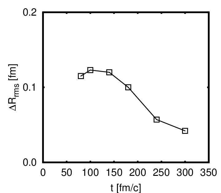
We also calculate the average of the difference of between the ensembles over a range of intermediate mass fragments (6–20);
| (12) |
We plot as a function of the reaction time in Fig. 12. The difference is large at the early stage of the reaction ( fm/) and reduces with time at the late stage of the reaction. In fact, the radii of the intermediate-mass fragments in the reaction ensemble at fm/ are larger than those in any of the equilibrium ensembles that we have investigated. This may be an indication of the fragment formation mechanism in which the fragments in the reaction are made from the expanding dilute system where surface effects are less important. It may also be related to the finding that the symmetry energy extracted from the multifragmentation reactions shows almost no surface effect [53].
VI Summary
In this paper, we have investigated the relevance of the equilibrium concept in multifragmentation by comparing reaction and equilibrium ensembles. The reaction ensemble at each reaction time is constructed by gathering the many-nucleon states at time in AMD simulations of very central collisions at 35 MeV/nucleon. The equilibrium ensemble is prepared by solving the AMD equation of motion of a many-nucleon system confined in a container for a long time. We then compare the reaction ensemble at each with equilibrium ensembles at various conditions of volume and energy. We have used exactly the same AMD model in simulating both situations. To our knowledge, this is the first work that directly compares the multifragmentation reaction and the corresponding equilibrium system by describing both situations with one model.
The AMD model used in this paper has been modified from that in Ref. [41] to better incorporate the effect of decoherence. We have confirmed the validity of the current version of AMD by comparing the result of reactions at 35 MeV/nucleon with the experimental data [51]. We have also confirmed that the constant-pressure caloric curves of the equilibrium system constructed with the same AMD show negative heat capacity which is the signal of the phase transition in finite systems.
The comparison between the reaction and equilibrium ensembles has been performed by computing the fragment charge distribution and the average excitation energies of fragments (fragment observables) for both ensembles. We are able to find an equilibrium ensemble that reproduces overall features at each reaction time 80–300 fm/. For the later stage of the reaction, an equilibrium ensemble with a larger volume and a slightly lower energy is required. This is consistent with the scenario that the system created by heavy-ion collisions cools during expansion. Unfortunately, it is difficult to identify the beginning and the end of the equivalence between the reaction and equilibrium systems, and it will be interesting to further develop the study to explore these. Experimentally, isotope thermometers have been utilized to extract the temperature from reactions [54, 55]. By comparing it with the temperature obtained by numerical simulation, it may be possible to identify the reaction stage relevant to the experimentally obtained isotope temperature.
The reaction ensembles have been constructed without any assumption of thermal equilibrium. Nevertheless, we can find an equilibrium ensemble that is almost equivalent to the reaction ensemble as far as the fragment observables are concerned at each reaction time after fm/. This is a rather surprising result, since there are certainly some observables that reflect the reaction dynamics. In fact, we have given several examples of the observables that show some discrepancy between the reaction and corresponding equilibrium ensembles. The fragment transverse kinetic energies are different from those of the equilibrium system, especially for the late stages of the reaction. However, the difference can be explained by simple flow effects. If the flow effects are subtracted, the fragment kinetic energies of the reaction system is still consistent with those of the equilibrium system. The size of the reaction system is larger than that of the equilibrium system. Namely, the real volume of the reaction system is larger than the volume assigned by fitting the fragment observables. The difference becomes larger at the later stages of the reaction. The usual static equilibrium at each instant is not realized since any equilibrium ensemble with the same volume as that of the reaction system cannot reproduce the fragment observables. The fragment radii in the reaction system are larger than those in the equilibrium system. The difference is large at the early stage of the reaction ( fm/) and decreases with time. This may be an indication of a fragment formation mechanism in which the fragments are made from an expanding dilute system in the reaction.
Only a small difference between the reaction and equilibrium ensembles is seen in the fragment observables studied in this paper. However, dynamical effects may become essential even for the fragment observables when the incident energy is increased or the impact parameter is varied. It has been suggested that neck formation play an important role in semiperipheral collisions [56], but in this paper we ignored this effect. It is an interesting question whether the equivalence between the multifragmentation reaction and the equilibrium system still holds under such circumstances. It is also interesting to compare observables such as the momentum distribution of fragments and the system size of multifragmentation reactions with those of the corresponding equilibrium systems in the explicit presence of expansion and flow effects [58, 57].
In this paper, we studied only one particular reaction, namely very central collisions at 35 MeV/nucleon. The reaction mechanism changes from one reaction to another. It is therefore interesting to apply the same approach to other reactions, such as a reaction of heavier nuclei where creation of a single thermal source is expected [44, 45], and a reaction of nuclei with different isospin compositions where the occurrence of isospin diffusion has been claimed[59, 60]. It is important to explore the effects of various reaction parameters such as the reaction system, the incident energy and the impact parameter on the achievement of equilibrium. If the concept of equilibrium is relevant, it is interesting to explore how these parameters influence the parameters to specify the equilibrium system. This study will offer guidelines for combining experimental data of various heavy-ion collisions to construct, for example, equation of states and constant-pressure caloric curves.
Acknowledgements.
The major part of this work has been done at Tohoku University as the Ph. D. study of T.F. T.F. acknowledges partial support from the ANR project NExEN (ANR-07-BLAN-0256-02). This work is partly supported by the High Energy Accelerator Research Organization (KEK) as a supercomputer project.APPENDIX: Improved implementation of decoherence
The reaction at 35 MeV/nucleon has already been studied by AMD [36, 23] and it has been shown that several aspects of the experimental data [51] are nicely reproduced. The AMD model used in these studies adopts the instantaneous decoherence of the single-particle motion [36]. In contrast, in Ref. [41] and in this paper, we utilize the AMD model in which the coherence of the single-particle motions are kept for a finite duration. When we directly applied the AMD formalism given in Ref. [41] to the reaction at 35 MeV/nucleon, excessive productions of heavy fragments are obtained and, connected to that, amounts of lighter fragments around the B-Ne region are underestimated compared with the experimental data. This is because the coherence time chosen by the formalism in Ref. [41] is too long and the effect of decoherence is hindered for some cases, and thus it fails to give enough quantum fluctuations to break the heavy fragments. A modification is necessary to better incorporate the effect of decoherence and reproduce the experimental data. This is rather technical but the summary is given in this Appendix.
In the AMD formalism, special care is taken for the nucleons that are almost isolated. For instance, the zero-point kinetic energies of these nucleons are subtracted since the wave functions of such nucleons should have sharp momentum distributions rather than Gaussian ones corresponding to the wave packet in Eq. (3). This change of interpretation is necessary for the consistency of Q-values of nucleon emissions and fragmentation [29, 28, 30] and is very important for the definition of temperature [41]. In Ref. [41], we judge the “degree of isolation” of the nucleon by introducing
| (13) |
where counts the neighboring nucleons of the nucleon including itself, is a continuous function from one when the number of neighboring nucleons is small () to zero, and corresponds to the inverse number of the neighboring nucleons. Detailed definitions of these functions are given in Appendix A in Ref. [41].
In the AMD formalism, the phase-space distribution is considered to compute the time evolution of the mean-field propagation. The distribution for each nucleon is parametrized by
| (14) |
where gives the six-dimensional phase-space coordinates
| (15) |
and and specify the shape and the centroids of the distribution, respectively. is identified with the physical coordinate [28, 29, 30]:
| (16) |
In Ref. [41], one condition was imposed on for each nucleon by using the degree of isolation . The condition was
| (17) |
where denotes the momentum spreading of the distribution . Namely, if the left-hand side of Eq. (17) is getting larger than the right-hand side, was reduced to satisfy the equality of Eq. (17) and the reduced part was converted into a stochastic Gaussian fluctuation to the centroid (the details are explained in Sec. III in Ref. [41]). The purpose of this condition is to ensure full consistency of the energy conservation and to allow precise evaluation of the temperature. When a recovery of the phase-space distribution for nucleon took place as a result of decoherence, we replaced the shape of the distribution with
| (18) |
where the momentum widths were chosen to be rather than the standard Gaussian width 1/4 to satisfy Eq. (17).
The condition is arbitrary as long as is satisfied for the nucleon that is utilized to measure the temperature. Unfortunately, it turns out that the condition (17) utilized in Ref. [41] tends to hinder the effect of decoherence unphysically at the surface of fragments. This is because increases close to unity when the nucleon is located near the surface of the fragment to which the nucleon belongs. The increase of results in keeping small, even though the recovery of the phase-space distribution defined by Eq. (18) frequently occurs. There is no physical reason why the effect of decoherence is suppressed at the surface of fragments and it is more natural that the effect of decoherence for the nucleon is as large as those for the other nucleons belonging to the same fragment even though the nucleon is located near the surface. We thus introduce a new function
| (19) |
and replace in Eq. (17) and Eq. (18) with this newly defined function , while we keep , which appears in the equation of motion as it is (see Sec. III in Ref. [41]). The difference between and is only that the first term of Eq. (13) is multiplied by so that when the nucleon is located inside of a fragment, whereas when the nucleon has only a few neighboring nucleons. In addition to this modification, we change the criteria to choose the nucleons that are used to measure temperature of the system. It has been shown that, to calculate the temperature of the system correctly, it is necessary to choose the subsystem consisting of the nucleons with negligible quantum effects among them based on only the nucleon spatial coordinates without using momentum variables (see Appendix B in Ref. [41]). For this purpose, there was a condition that the nucleons that are used to measure the temperature are chosen not to have more than one other nucleon within a distance of 3 fm in Ref. [41]. We replace this condition with , which has similar meaning to the aforementioned condition and guarantees that the difference between and for these nucleons is at most. This replacement is justified by the study that the measured temperatures are independent of the choice of nucleons utilized to measure the temperature as long as necessary conditions are satisfied (see Sec. VC in Ref. [41]).
References
- [1] C. P. Montoya et al., Phys. Rev. Lett. 73, 3070 (1994).
- [2] J. Lukasik et al., Phys. Rev. C 55, 1906 (1997), and references therein.
- [3] T. Lefort et al., Nucl. Phys. A662, 397 (2000).
- [4] W. Reisdorf et al., Nucl. Phys. A612, 493 (1997).
- [5] J. Pochodzalla et al., Phys. Rev. Lett. 75, 1040 (1995).
- [6] P. Danielewicz, R. Lacey, and W. G. Lynch, Science 298, 1592 (2002).
- [7] C. Fuchs and H. H. Wolter, Eur. Phys. J. A 30, 5 (2006), and references therein.
- [8] C. J. Horowitz, Eur. Phys. J. A 30, 303 (2006), and references therein.
- [9] S. Das Gupta, A. Z. Mekjian, and M. B. Tsang, Adv. Nucl. Phys. 26, 89 (2001).
- [10] M. D’Agostino et al., Nucl. Phys. A650, 329 (1999).
- [11] M. D’Agostino et al., Phys. Lett. B473, 219 (2000).
- [12] J. B. Natowitz et al., Phys. Rev. C 65, 034618 (2002).
- [13] J. B. Elliott et al., Phys. Rev. Lett. 88, 042701 (2002).
- [14] W. Trautmann, Nucl.Phys. A752, 407 (2005), and references therein.
- [15] Ph. Chomaz and F. Gulminelli, Nucl. Phys. A647, 153 (1999).
- [16] H. S. Xu et al., Phys. Rev. Lett. 85, 716 (2000).
- [17] M. B. Tsang et al., Phys. Rev. C 64, 054615 (2001).
- [18] D. H. E. Gross, Phys. Rep. 279, 120 (1997).
- [19] J. Randrup and S. E. Koonin, Nucl. Phys. A471, 355 (1987).
- [20] J. P. Bondorf, A. S. Botvina, A. S. Iljinov, I. N. Mishustin, and K. Sneppen, Phys. Rep. 257, 133 (1995).
- [21] M. D’Agostino et al., Phys. Lett. B371, 175 (1996).
- [22] A. S. Botvina and I. N. Mishustin, Eur. Phys. J. A 30, 121 (2006), and references therein.
- [23] R. Wada et al., Phys. Lett. B422, 6 (1998).
- [24] N. Marie et al., Phys. Lett. B391, 15 (1997).
- [25] P. Désesquelles et al., Nucl. Phys. A633, 547 (1998).
- [26] W. Reisdorf and H. G. Ritter, Annu. Rev. Nucl. Part. Sci. 47, 663 (1997).
- [27] A. Andronic, J. Lukasik, W. Reisdorf, and W. Trautmann, Eur. Phys. J. A 30, 31 (2006), and references therein.
- [28] A. Ono, H. Horiuchi, T. Maruyama, and A. Ohnishi, Phys. Rev. Lett. 68, 2898 (1992).
- [29] A. Ono, H. Horiuchi, T. Maruyama, and A. Ohnishi, Prog. Theor. Phys. 87, 1185 (1992).
- [30] A. Ono and H. Horiuchi, Prog. Part. Nucl. Phys. 53, 501 (2004).
- [31] A. Ono, Phys. Rev. C 59, 853 (1999).
- [32] A. Ono, S. Hudan, A. Chbihi, and J. D. Frankland, Phys. Rev. C 66, 014603 (2002).
- [33] R. Wada et al., Phys. Rev. C 62, 034601 (2000).
- [34] R. Wada et al., Phys. Rev. C 69, 044610 (2004).
- [35] S. Hudan, R. T. de Souza, and A. Ono, Phys. Rev. C 73, 054602 (2006).
- [36] A. Ono and H. Horiuchi, Phys. Rev. C 53, 2958 (1996).
- [37] A. Ohnishi and J. Randrup, Phys. Rev. Lett. 75, 596 (1995).
- [38] A. Ohnishi and J. Randrup, Ann. Phys. 253, 279 (1997).
- [39] A. Ono and H. Horiuchi, Phys. Rev. C 53, 845 (1996).
- [40] A. Ono and H. Horiuchi, Phys. Rev. C 53, 2341 (1996).
- [41] T. Furuta and A. Ono, Phys. Rev. C 74, 014612 (2006).
- [42] D. H. E. Gross and E. V. Votyakov, Eur. Phys. J. B 15, 115 (2000).
- [43] D. H. E. Gross, Phys. Chem. Chem. Phys. 4, 863 (2002).
- [44] A. H. Raduta, M. Colonna, V. Baran, and M. Di Toro, Phys. Rev. C 74, 034604 (2006).
- [45] A. H. Raduta, M. Colonna, and M. Di Toro, Phys. Rev. C 76, 024602 (2007).
- [46] M. Colonna, G. Fabbri, M. Di Toro, F. Matera, and H. H. Wolter, Nucl. Phys. A742, 337 (2004).
- [47] A. H. Raduta and A. R. Raduta, Phys. Rev. C 65, 054610 (2002).
- [48] A. Ono, H. Horiuchi, and T. Maruyama, Phys. Rev. C 48, 2946 (1993).
- [49] Y. Kanada-En’yo, Phys. Rev. C 71, 014310 (2005), and references therein.
- [50] J. Dechargé and D. Gogny, Phys. Rev. C 21, 1568 (1980).
- [51] K. Hagel et al., Phys. Rev. C 50, 2017 (1994).
- [52] T. Maruyama, A. Ono, A. Ohnishi, and H. Horiuchi, Prog. Theor. Phys. 87, 1367 (1992).
- [53] A. Ono, P. Danielewicz, W. A. Friedman, W. G. Lynch, and M. B. Tsang, Phys. Rev. C 70, 041604(R) (2004).
- [54] S. Albergo, S. Costa, E. Costanzo, and A. Rubbino, Nuovo Cimento A 89, 1 (1985).
- [55] W. P. Tan, S. R. Souza, R. J. Charity, R. Donangelo, W. G. Lynch, and M. B. Tsang, Phys. Rev. C 68, 034609 (2003).
- [56] M. Di Toro, A. Olmi, and R. Roy, Eur. Phys. J. A 30, 65 (2006), and references therein.
- [57] M. J. Ison, F. Gulminelli, and C. O. Dorso, Phys. Rev. E 76, 051120 (2007).
- [58] F. Gulminelli and Ph. Chomaz, Nucl. Phys. A734, 581 (2004).
- [59] M. B. Tsang et al., Phys. Rev. Lett. 92, 062701 (2004).
- [60] Lie-Wen Chen, Che Ming Ko, and Bao-An Li, Phys. Rev. Lett. 94, 032701 (2005).