Joint Transmitter-Receiver Design for the Downlink Multiuser Spatial Multiplexing MIMO System

Spatial multiplexing for the multiple-input multiple-output (MIMO) systems, employing multiple transmit and receive antennas, has been recognized as an effective way to improve the spectral efficiency of the wireless link [1]. More recently, the multiuser schemes have been investigated for the spatial multiplexing MIMO systems. This paper focuses on the downlink multiuser schemes in which each user can not cooperate with the others thus suffers from the interference from them.

Mainly, there are two kinds of multiuser schemes. One is the precoder or the transmit beamforming, such as the dirty-paper coding (DPC) [2] and the zero-forcing (ZF) [3], etc., which mitigates the multiuser interference only by processing at the transmitter. The other is the joint transmitter-receiver (Tx-Rx) design, such as the nullspace-directed SVD (Nu-SVD) [4] and the minimum total mean squared error (TMMSE) [5], etc. In general, the former possesses lower complexity but more performance penalty. With the great development of signal processors, the latter gradually draws more attention.

For the joint Tx-Rx design, the schemes proposed in [4][5] minimize mean squared error (MMSE), or maximize the capacity under the transmit power constraint. Whereas on some occasions, such as the multimedia communication, it is required to minimize the total transmit power while guarantee the quality of service (QoS). [6][7] investigate the beamforming and the power allocation policy when all users are subjected to a set of post-processing signal-to-interference-and-noise ratio (post-SINR) constrains in the uplink SIMO and the downlink MISO. [8][9] extend this work to the downlink MIMO and the MIMO network, however the MIMO systems discussed in [8][9] are assumed that there is only one substream between each pair of the transmitter and receiver. In other words, only the multiuser interference appears in the so-called diversity MIMO system in [8][9]. For the multiuser spatial multiplexing MIMO system, however, both the multiuser interference between individual users and self-interference between individual substreams of a user should be mitigated.

For the downlink, the transmit beamforming affects the interference signature of all receivers, whereas the receive beamforming only affects that of the corresponding user. [7][8] construct a dual system, called the virtual uplink, and indicate that the virtual uplink can obtain the same post-SINR as the primary downlink. Moreover, the receive beamforming matrix of the virtual uplink is identical with the transmit beamforming matrix of the primary downlink. The design of the downlink, therefore, can resort to the virtual uplink.

In this paper, we extend the duality derived for MIMO network in [9] to the multiuser spatial multiplexing MIMO system. According to the uplink-downlink duality, we propose a joint Tx-Rx scheme to minimize the weighted sum power under the post-SINR constraints of all the subchannels.

Notation: Boldface upper-case letters denote matrices, and boldface lower-case letters denote column vectors. $tr(\cdot)$, $(\cdot)^{*}$, $(\cdot)^{H}$, $||\cdot||_{2}$ and $||\cdot||_{F}$ denote trace, conjugate, conjugate transposition, Euclidian norm and Frobenius norm, respectively. $diag({\bf{x}})$ denotes a diagonal matrix with diagonal elements drawn from the vector ${\bf{x}}$. $[{\bf{\cdot}}]_{i,j}$, $[{\bf{\cdot}}]_{{\bf{:}},j}$ denote the $(i$,$j)$-th element and $j$-th column of a matrix, respectively.

We consider a base station (BS) with $M$ antennas and $K$ mobile stations (MS’s) each having $N_{i}(i=1,\ldots,K)$ antennas. There are $L_{i}(i=1,\ldots,K)$ substreams between BS and MS${}_{i}(i=1,\ldots,K)$, that is to say, BS transmits $L_{i}$ symbols to MS_i simultaneously. The signal recovered by MS_k can be written as

where $\mathbf{y}_{k}^{DL}\in\mathcal{C}^{L_{k}\times 1}$ is the recovered signal vector. $\mathbf{x}_{i}\in\mathcal{C}^{L_{i}\times 1}(i=1,\ldots,K)$ is the transmitted signal vector from BS to MS_i with zero-mean and normalized covariance matrix $\mathbf{I}$. $\mathbf{p}_{i}\in\mathcal{R}^{L_{i}\times 1}$ denotes the power vector allocated to MS_i. A linear post-filter $\mathbf{A}_{k}\in\mathcal{C}^{N_{k}\times{L_{k}}}$ is used to recover an estimation of the transmitted signal vector $\mathbf{x}_{k}$. The MIMO channel from BS to MS_k is denoted as $\mathbf{H}_{k}\in\mathcal{C}^{N_{k}\times M}$, and assumed flat faded. Hence, its elements are the complex channel gains, and they are independently identically distributed (i.i.d.) zero-mean complex Gaussian random variables with the unity variance. Moreover, the perfect channel state information are assumed available at both transmitter and receiver via some way, for example, channel measurement at receiver and fast feedback to the transmitter for the frequency division duplex (FDD) systems, or invoking the channel reciprocity in time division duplex (TDD) systems. $\mathbf{B}_{i}\in\mathcal{C}^{M\times L_{i}}$ is used to weight $\mathbf{x}_{i}$ and transform it into a $M\times 1$ vector. $\mathbf{n}_{k}\in\mathcal{C}^{N_{k}\times 1}$ is the noise vector with the correlation matrix $\mathbf{R}_{n}=\sigma_{n}^{2}\mathbf{I}$. For simplicity, in the sequel we assume $L_{1}=\ldots=L_{K}=L$.

We design the $\mathbf{A}_{k}$, $\mathbf{B}_{k}$ and $\mathbf{p}_{k}(k=1,\ldots,K)$ in (1) to minimize the weighted sum power under the post-SINR constraints, which can be denoted as the following optimization problem.

where ${\bf{p}}=[{\bf{p}}_{1}^{T},\ldots,{\bf{p}}_{K}^{T}]^{T}$ and $\mathbf{w}\in\mathcal{R}^{KL\times 1}$ is the weight vector. $\mathbf{w}$ affects the power distribution among users, and its value is determined by various factors, such as the positions of users in a cell and the interference environment of the neighboring cells. $\gamma_{k,j}$ is the given post-SINR goal for the MS_k’s $j$-th substream.

If ${\bf{A}}_{k}=\left[{{\bf{a}}_{k,1}},{\ldots},{{\bf{a}}_{k,L}}\right]$, ${\bf{B}}_{k}=\left[{{\bf{b}}_{k,1}},{\ldots},{{\bf{b}}_{k,L}}\right]$, ${\bf{p}}_{k}=\left[{p_{k,1}},{\ldots},{p_{k,L}}\right]^{T}$, (1) can be rewritten into

The diagonal elements of the first part in the right-hand side (RHS) of (3) denote the useful signals, and the non-diagonal elements denote the self-interference. The medial and the last parts in the RHS of (3) denote the multiuser interference and the noise, respectively. Moreover, the post-SINR of the MS_k’s $j$-th substream can be denote as

If ${\bf{x}}_{m}=\left[{x_{m,1}},{\ldots},{x_{m,L}}\right]$, ${\bf{y}}_{k}^{DL}=\left[{y_{k,1}},{\ldots},{y_{k,L}}\right]$, the link power gain between $x_{m,n}$ and $y_{k,j}$ can be denoted as

then (4) can be rewritten into

By substituting (6) into the constraint inequality of (2), we obtain

where the $m$-th element of $\mathbf{c}_{k,j}\in\mathcal{R}^{KL\times 1}$ is

where $\left\lceil{\frac{m}{L}}\right\rceil$ rounds $\frac{m}{L}$ to the nearest integer greater than or equal to $\frac{m}{L}$ . Write (7) into the matrix form, we obtain

where $\mathbf{C}\in\mathcal{R}^{KL\times KL}$ and $\mathbf{d}\in\mathcal{R}^{KL\times 1}$ are

So, (2) is equivalent to the following optimization problem

Subsequently, to obtain the Lagrangian duality of (11) [9], we divide the solving process of (11) into two steps similar with [10]. First, assuming ${\bf{A}}_{k}$ and ${\bf{B}}_{k}(k=1,\ldots,K)$ are fixed, the Lagrangian function of (11) is

where ${\mbox{\boldmath{$\lambda$}}}\geq{\bf{0}}$, ${\mbox{\boldmath{$\mu$}}}\geq{\bf{0}}$ are the Lagrangian multipliers associated with the inequality constraints. Then the Lagrangian duality of (11) is

According to the Slater’s condition, (11) is equivalent to (13). Since the gradient of the Lagrangian function (12) with respect to $\bf{p}$ vanishs at optimal points, we obtain ${\bf{w}}^{T}-{\mbox{\boldmath{$\mu$}}}^{T}=-{\mbox{\boldmath{$\lambda$}}}^{T}{\bf{C}}$. Substituting it into (12), we obtain $\mathop{\min}\limits_{\bf{p}}L({\bf{p}},{\mbox{\boldmath{$\lambda$}}},{\mbox{\boldmath{$\mu$}}})={\bf{d}}^{T}{\mbox{\boldmath{$\lambda$}}}$. Moreover, as ${\mbox{\boldmath{$\lambda$}}}\geq{\bf{0}}$ and ${\mbox{\boldmath{$\mu$}}}\geq{\bf{0}}$, (13) can be rewritten to

Similar with (6)-(9), substitute (10) into (14), we obtain

where

where ${\mbox{\boldmath{$\lambda$}}}=[{\mbox{\boldmath{$\lambda$}}}_{1}^{T},\ldots,{\mbox{\boldmath{$\lambda$}}}_{K}^{T}]$. Furthermore, $SINR_{k,j}^{UL}$ is the post-SINR of MS_k’s $j$-th substream in the virtual uplink

(14) maximizes the weighted sum power under the maximum post-SINR constraints, however, it has no physical meaning [9]. But it can be shown that (14) is equivalent to the following optimization problem

Theorem 1: At the optimal point, the post-SINR constraints in (15) and (18) are active. And the solutions of (15) and (18) are identical.

Proof: Without any loss of the generality, we assume $SINR_{k,j}^{UL}<\gamma_{k,j}$. From (16), we can find $\lambda_{k,j}$ contribute to the numerator of $SINR_{k,j}^{UL}$ and the denominator of $SINR_{m,n}^{UL}(m\neq k,n\neq j)$. In other words, $SINR_{k,j}^{UL}$ is a monotone increasing function of $\lambda_{k,j}$, while $SINR_{m,n}^{UL}(m\neq k,n\neq j)$ is a monotone decreasing function of $\lambda_{k,j}$. So increasing $\lambda_{k,j}$ until $SINR_{k,j}^{UL}=\gamma_{k,j}$, we obtain a larger ${\bf{d}}^{T}{\mbox{\boldmath{$\lambda$}}}$ without breaking any post-SINR constraint. Likewise, if $SINR_{k,j}^{UL}>\gamma_{k,j}$, decreasing $\lambda_{k,j}$ until $SINR_{k,j}^{UL}=\gamma_{k,j}$, a smaller ${\bf{d}}^{T}{\mbox{\boldmath{$\lambda$}}}$ is obtained. As a result, the constraints of (15) and (18) become a linear equations ${\bf{C}}^{T}{\mbox{\boldmath{$\lambda$}}}+{\bf{w}}={\bf{0}}$, and its solution is ${\mbox{\boldmath{$\lambda$}}}^{*}=-({\bf{C}}^{T})^{-1}{\bf{w}}$.

Similar with Theorem 1, at the optimal point of (11) ${\bf{p}}^{*}=-{\bf{C}}^{-1}{\bf{d}}$.

Summarize the above statement, we obtain the following conclusion.

Theorem 2: In the downlink multiuser spatial multiplexing MIMO system, if the transmit and receive beamforming matrices are ${\bf{B}}_{k}$ and ${\bf{A}}_{k}^{H}(k=1,\ldots,K)$, respectively, as long as the following conditions are satisfied, the downlink optimization problem (2) is equivalent to the virtual uplink optimization problem (18).

1) In the virtual uplink, the transmit and receive beamforming matrices are ${\bf{A}}_{k}$ and ${\bf{B}}_{k}^{H}(k=1,\ldots,K)$, respectively.

2) In the virtual uplink problem (18), the weight vector ${\bf{w}}$ is the noise power vector.

3) In the virtual uplink problem (18), the noise power vector ${\bf{d}}$ is the weight vector.

When ${\bf{A}}_{k}$ and ${\bf{B}}_{k}(k=1,\ldots,K)$ are not fixed, (18) is a joint optimization problem denoted as

Theorem 3: If the noise power vector in the virtual uplink is the weight vector ${\bf{w}}$, the joint optimization problem (2) is equivalent to (19). At the optimal point, the beamforming matrices of the virtual uplink and the primal downlink are common.

Proof: Let ${({\bf{B}}_{k}^{*},{\bf{A}}^{*}_{k},{\bf{p}}^{*})}\;(k=1,\ldots,K)$ be the global minimum of (2). According to Theorem 2, (19) has the solution ${({\bf{A}}_{k}^{*},{\bf{B}}^{*}_{k},{\mbox{\boldmath{$\lambda$}}}^{*})}\;{k=1,\ldots,K}$. Moreover, this solution is definitely the global minimum. Otherwise, a better solution of (2) would be found by applying Theorem 2 again. So the virtual uplink and the primal downlink have the common beamforming matrices.

The weight vector ${\bf{w}}$ decides whether ${\bf{A}}_{k}$ and ${\bf{B}}_{k}$ are used to strengthen the useful signals or alleviate the interference to other users. When a user’s weight turns higher, its transmit power will decrease. In this occasion, it benefits to apply the beamforming to increase the signal gain, as the interference to other users is much less important. On the other hand, once the weight gets lower, the beamformer should try to suppress interference to others [9].

To mitigate the adjacent cell interference, we can increase the weights of edge users in a cell, which would induce the declining of the transmit power from the BS to them. In order to hold the post-SINR under this circumstance, obviously, the beamforming matrices would be used to boost up the signal gain.

It is rather difficult to solve the joint optimization problem (2) directly. However, it is easy to obtain ${\bf{A}}_{k}(k=1,\ldots,K)$ in the primal downlink, and so does ${\bf{B}}_{k}(k=1,\ldots,K)$ in the virtual uplink. Moreover, it is proved in the previous section that the primal downlink is equivalent to the virtual uplink, and they have the common beamforming matrices ${\bf{A}}_{k}$ and ${\bf{B}}_{k}(k=1,\ldots,K)$. Therefore, we divide the solving process into four steps shown as Fig. 1.

When ${\bf{p}}$ and ${\bf{B}}_{k}(k=1,\ldots,K)$ are fixed, optimize ${\bf{A}}_{k}(k=1,\ldots,K)$ to maximize $SINR_{k,j}^{DL}(k=1,\ldots,K,j=1,\ldots,L)$. Then observing (4), it is a generalized Rayleigh quotient problem, and its solution is

where $\xi_{\max}({\bf{X}}$,${\bf{Y}})$ is the dominant generalized eigenvector of the matrix pair $({\bf{X}}$,${\bf{Y}})$. When $\lambda$ and ${\bf{A}}_{k}(k=1,\ldots,K)$ are fixed, in the same way, ${\bf{B}}_{k}(k=1,\ldots,K)$ can be obtained by

The proposed algorithm is summarized in the following.

By iteration, ${({\bf{A}}_{k}^{(n+1)},{\bf{B}}_{k}^{(n+1)},{\bf{p}}^{(n+1)})}{(k=1,\ldots,K)}$ converges to the optimal solution to the optimization problem (2).

Once any element in ${\bf{p}}^{(n+1)}$ is negative, which indicates the post-SINR goals ${\gamma}_{k,j}(k=1,\ldots,K,j=1,\ldots,L)$ can not be attained, ${\gamma}_{k,j}$ should be decreased to relax the post-SINR constraints. When $\bf{w}=\bf{1}$, the proposed algorithm is similar with the one in [11].

In this section, we assume that a BS with $8$ antennas ($M=8$) is communicating with $K$ MS’s each with $2$ antennas, $(N_{1}=\ldots=N_{K}=2)$. Also we assume that the number of substreams of each MS is the same, equal to $2$,$(L_{1}=\ldots=L_{K}=2)$. QPSK is employed in the simulation and no forward error coding is considered. The post-SINR goals for all substreams are $\gamma({\gamma_{k,j}=\gamma})$. Additionally we assume MS₁ is an edge user in a cell, according to the previous section, a higher weight should be assigned to it to mitigate the adjacent cell interference. Thus, the weight vector is set to ${\bf{w}}=[w,w,1,\ldots,1]^{T}$, where $w$ is the weight corresponding to the two substreams of MS₁ and $w>1$.

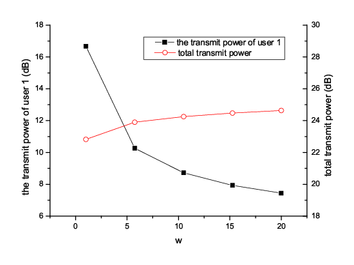
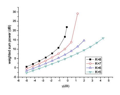
Fig. 2,3 plot the curves of the total transmit power ${\sum\limits_{k,j}{p_{k,j}}}$ versus the post-SINR goal $\gamma$, when $w=5$. In Fig. 2, $K=2,3,4$, the system configuration satisfies $M\geq KL$, the multiuser interference, thus, can be effectively suppressed through the beamforming [4]. Under the circumstance, increasing the transmit power of any user has nearly no effect to the post-SINR of other users. Therefore, all the substreams can attain relatively high post-SINR. In Fig. 3, $K=5,6,7,8$, $M\geq KL$ does not hold any more. Consequently, the multiuser interference can not be effectively mitigated, which means any enhancement in the transmit power of any user is very likely to deteriorate the post-SINR of other users. As shown in Fig. 3, with the user number increasing, the available post-SINR of each user is decreased. When $K=8$, only $0$ dB post-SINR can be attained. In these two figures, the total transmit power increases with the number of users and the post-SINR goal $\gamma$. Especially when $K=7,8$ and $\gamma\geq 0$ dB in Fig. 3, due to the residual multiuser interference, the slopes of the curves are much steeper than that in Fig. 2 where the multiuser interference is negligible. And the steeper the curves are, the more power would be paid for the unit increase of the post-SINR of each user.

Fig. 4 shows the curves of the transmit power ${\sum\limits_{j}{p_{1,j}}}$ of MS₁ and the total transmit power ${\sum\limits_{k,j}{p_{k,j}}}$ versus the weight $w$, when $K=4$ and $\gamma=10$dB. The left vertical axis is corresponding to the transmit power of MS₁ and the right one is to the total transmit power. Obviously, as the $w$ is increasing, the transmit power of MS₁ is decreasing while the total power is increasing, because the optimization object is to minimize the weighted sum power ${\sum\limits_{k,j}{w_{k,j}p_{k,j}}}$. Moreover, when $w$ changing from $1$ to $20$, the transmit power of MS₁ decreases almost $10$dB, however the total power increases only about $1$ dB, which demonstrates that the proposed algorithm adapts the power allocation policy very effectively with negligible penalty on performance.

In this paper, we investigate the joint Tx-Rx design for the downlink multiuser spatial multiplexing MIMO system. We show, first, the uplink-downlink duality has the following characteristics: 1) In both of the primal downlink and the virtual uplink, the substreams can attain the same post-SINR goal; 2) The beamforming matrices are common in both of the primal downlink and the virtual uplink.

Based on the duality, a joint Tx-Rx beamforming scheme is proposed. Simulation results demonstrate that the scheme can not only satisfy the post-SINR constraints which guarantee the performance of the communication links, but also easily adjust the power distribution among users by changing the weights correspondingly, which can be used to diminish the power of the edge users in a cell to alleviate the adjacent cell interference.

References

- [1] I. Telatar, ”Capacity of multi-antenna Gaussian channels”, Eur. Trans. Telecommun, vol. 10, no. 6, pp.585-595, Nov./Dec. 1999.
- [2] Q. Caire and S. Shamai, ”On the achievable throughput of a multiantenna gaussian broadcast channel”, IEEE Trans. Inform. theory, vol. 49, no. 7, pp.1691-1706, July 2003.
- [3] Q. Spencer, A. Swindlehurst and M. Haardt, ”Zero-forcing methods for downlink spatial multiplexing in multiuser mimo channels”, IEEE Trans. Signal Processing, vol. 52, no. 2, pp.461- 471, Feb. 2004.
- [4] Z.G. Pan,K.K. Wong and T.S. Ng, ”Generalized multiuser orthogonal space division multiplexing”, IEEE Trans. Wireless Commun., vol. 3, no. 6, pp.1969- 1973, Nov. 2004.
- [5] J. Zhang, Y. Wu, S. Zhou and J. Wang, ”Joint linear transmitter and receiver design for the downlink of multiuser MIMO systems”, IEEE commun. Lett, vol.9, pp.991-993, Nov. 2005.
- [6] F. Rashid-Farrokhi, L. Tassiulas, and K.J Liu, ”Joint optimal power control and beamforming in wireless networks using antenna array”, IEEE Trans. Commun., vol. 46, no. 11, pp.1313-1324, Nov. 1998.
- [7] F. Rashid-Farrokhi F., K.J. Liu and L. Tassiulas, ”Transmit beamforming and power control for cellular wireless systems”, IEEE J. Sel. Areas Commun., vol. 16, no. 8, pp.1437-1450, Oct. 1998.
- [8] J.H. Chang, L. Tassiulas and F. Rashid-Farrokhi, ”Joint transmitter receiver diversity for efficient space division multiaccess”, IEEE Trans. Wireless Commun., vol. 1, no. 1, pp.16-27, Jan. 2002.
- [9] S. Boyd and L. Vandenberghe, Convex Optimization, Cambridge: U.K. Cambridge University Press, 2004.
- [10] B. Song, R.L. Cruz and B.D. Rao, ”Network Duality for Multiuser MIMO Beamforming Networks and Applications”, IEEE Trans. Commun., vol.55, no.3, pp.618-629, Mar. 2007.
- [11] A.M. Khachan, A.J. Tenenbaum and R.S. Adve, ”Linear Processing for the Downlink in Multiuser MIMO Systems with Multiple Data Streams”, IEEE ICC’06, vol. 9, pp.4113-4118, June 2006.