A novel generalization of Clifford’s classical point-circle configuration. Geometric interpretation of the quaternionic discrete Schwarzian KP equation
Abstract
Clifford configurations; quaternions; multi-ratios; integrable systems; discrete differential geometry The algebraic and geometric properties of a novel generalization of Clifford’s classical point-circle configuration are analysed. A connection with the integrable quaternionic discrete Schwarzian Kadomtsev-Petviashvili equation is revealed.
1 Introduction
In his seminal paper Clifford’s chain and its analogues in relation to the higher polytopes, Longuet-Higgins (1972) asserts that ”a chain of theorems … has exerted a peculiar fascination for mathematicians since its discovery by Clifford in 1871”. Indeed, various generalizations and analogues in higher dimension of Clifford’s point-circle configurations (Clifford 1871) associated with such luminaries as de Longechamps (1877), Cox (1891), Grace (1898), Brown (1954), Coxeter (1956) and Longuet-Higgins (1972) have been recorded and analysed in detail. The original celebrated chain of ‘circle theorems’ may be stated as follows:
Given four straight lines on a plane, the four circumcircles of the four triangles so formed are concurrent in a point , say (cf. figure 1).
Given five lines on a plane, by omitting each line in turn, we obtain five corresponding points and these lie on a circle , say.
Given six lines on a plane, we obtain six corresponding circles and these are concurrent in a point .
Etc.
Generally, given coplanar lines, we obtain corresponding circles which are concurrent in a point or points which lie on a circle depending on whether is even or odd respectively.
Finally, application of an inversion with respect to a generic point on the plane leads to a complete and symmetric configuration of points and circles with points on every circle and circles through every point.

The first theorem associated with four straight lines immediately demonstrates that there exists a close connection between Clifford configurations and the ancient Theorem of Menelaus (Pedoe 1970). The latter states that three points on the (extended) edges of a triangle with vertices as displayed in figure 1 are collinear if and only if the condition
| (1) |
for the associated directed lengths is satisfied. Accordingly, the points of intersection of the four lines in Clifford’s first theorem (see figure 1) obey condition (1). If the plane is identified with the complex plane then condition (1) constitutes a multi-ratio condition for the complex numbers which we denote by (cf. §2)
| (2) |
(modulo a trivial cyclic permutation of the arguments). The latter is evidently invariant under the group of inversive transformations (Brannan et al. 1999) and hence the points of a Clifford configuration likewise satisfy the multi-ratio condition (2). In fact, it has been pointed out in Konopelchenko & Schief (2002) that the latter constitutes a defining property of Clifford configurations.
In this paper, we investigate in detail the geometric and algebraic properties of a novel generalization of Clifford’s configuration which has been discovered via the theory of integrable systems (soliton theory) (Ablowitz & Segur 1981; Zakharov et al. 1980). Thus, in Konopelchenko & Schief (2002), it has been shown that (2) interpreted as a lattice equation which is defined on the ‘octahedral’ vertex configurations of a face-centred cubic (fcc) lattice (cf. §7) constitutes a Schwarzian version (Dorfman & Nijhoff 1991; Bogdanov & Konopelchenko 1998) of the Hirota-Miwa equation, that is the discrete Kadomtsev-Petviashvili (dKP) equation (Hirota 1981). The latter is regarded as a ‘master equation’ in soliton theory since it encodes the complete KP hierarchy of soliton equations via sophisticated continuum limits. The discrete Schwarzian KP (dSKP) equation admits a natural multi-component analogue, namely the natural matrix generalization of the multi-ratio condition (2) interpreted as a lattice equation (Bogdanov & Konopelchenko 1998). In the simplest case, the quaternionic dSKP (qdSKP) equation locally represents a six-point relation for six quaternions , that is, a relation between six points in a four-dimensional Euclidean space if the standard identification with the algebra of quaternions is made. Since the multi-ratio condition (2) encodes Clifford configurations, it is natural to inquire as to the geometric significance of its quaternionic counterpart. It turns out that an appropriate characterization of classical Clifford configurations gives rise to natural analogues in a four-dimensional Euclidean space which are algebraically governed by the local qdSKP equation.
In the present context, the key property of classical Clifford configurations turns out to be the Godt-Ziegenbein property which states that, in a specific sense, the angles made by four oriented circles passing through a point are the same for all eight points (Godt 1896; Ziegenbein 1941). This property is used in §3 to define octahedral point-circle configurations in of Clifford type. In §6, the existence of such generalized Clifford configurations is proven and it is demonstrated that these are indeed governed by the afore-mentioned quaternionic version of the multi-ratio condition (2). As a by-product, it is shown that, for any five generic points in , there exists a pair of associated generalized Clifford configurations which are related by reflection in the hypersphere defined by the given five points. The final section is then devoted to the geometry of the qdSKP (lattice) equation.
2 The classical Clifford configuration
We begin with the classical construction of Clifford configurations. Thus, consider a point on the plane and four generic circles passing through as depicted in figure 2. The six additional points of intersection are labelled by . Here, the indices on correspond to those of the circles and . Any three circles intersect at three points and therefore define a circle passing through these points. Clifford’s circle theorem (Clifford 1871) then states that the four circles meet at a point . Even though Clifford configurations () exist for any number of initial circles passing through a point , for brevity, we here associate with the term ‘Clifford configuration’ the case .

In Konopelchenko & Schief (2002), as an immediate consequence of the classical Theorem of Menelaus (Pedoe 1970), it has been demonstrated that any generic six points , on the plane regarded as complex numbers belong to a Clifford configuration (with the above-mentioned combinatorics) if and only if they obey the multi-ratio condition
| (3) |
where the multi-ratio of six complex numbers is defined by
| (4) |
In particular, this confirms the geometrically evident fact that any five generic points on the plane uniquely define a Clifford configuration. Indeed, for any given generic points , the sixth point is determined by the linear equation (3). The latter point may lie ‘at infinity’, in which case the four circles passing through degenerate to straight lines. The justification of the ordering of the arguments in (3) is consigned to §6.
The preceding discussion indicates that one may think of a Clifford configuration as a configuration of six points and eight circles which is such that the four circles intersect at a point or the four circles intersect at a point . Clifford’s circle theorem then guarantees the existence of the remaining point or respectively. In this connection, it is noted that the eight points of a Clifford configuration appear on an equal footing so that, at first sight, the above interpretation of a Clifford configuration does not seem to be natural. However, it turns out that it is precisely this point of view which allows for a generalization of Clifford configurations in which, generically, the points and do not exist.
A remarkable property of Clifford configurations is that the angles made by four oriented circles passing through a point are the same for all eight points in a sense to be specified in the following section. Therein, it is shown that this Godt-Ziegenbein property (Godt 1896; Ziegenbein 1941) constitutes a defining property of Clifford configurations. In fact, it is sufficient to demand that the Godt-Ziegenbein property holds for the points . The latter observation serves as the basis for the definition of generalized Clifford configurations.
3 Octahedral point-circle configurations. Definitions and notation
In the following, we are concerned with configurations in a four-dimensional Euclidean space consisting of six points and eight circles with three points on every circle and four circles through every point. More precisely (cf. figure 3):
Definition \thetheorem.
(Octahedral point-circle configurations) A configuration of six points and eight circles in is termed an octahedral point-circle configuration if the combinatorics of the configuration is that of an octahedron, that is the points of the configuration correspond to the vertices of the octahedron while the circles correspond to the triangular faces.

In order to define octahedral point-circle configurations of Clifford type, it is necessary to introduce a correspondence between circles which pass through different points. To this end, we observe that any vertex of an octahedron may be associated with its ‘opposite’ counterpart, that is the vertex which is not connected via an edge. Similarly, there exist four pairs of disconnected ‘opposite’ faces. Thus, by virtue of the combinatorial correspondence employed in the above definition, any point of an octahedral point-circle configuration admits an ‘opposite’ point and any circle is associated with an ‘opposite’ circle (cf. figure 4).

Definition \thetheorem.
(Correspondence of circles) Let and be points and circles of an octahedral point-circle configuration such that and intersect at and and lies on . Then, the circles and passing through are said to correspond to the circles and respectively passing through and the circle passing through is said to correspond to the opposite circle passing through the opposite point :
| (5) |
Iterative application of the above correspondence principle immediately leads to the following correspondence:
Observation \thetheorem.
Any circle of an octahedral point-circle configuration passing through a point admits five corresponding circles which pass through the remaining five points . Thus, there exists a unique correspondence between the six sets of four circles passing through the points of an octahedral point-circle configuration.
Convention \thetheorem.
(Orientation of circles) The orientation of the circles of an octahedral point-circle configuration is chosen in such a manner that the corresponding orientation of the faces of the octahedron is the same for all faces (when viewed from ‘outside’) (cf. figure 5).
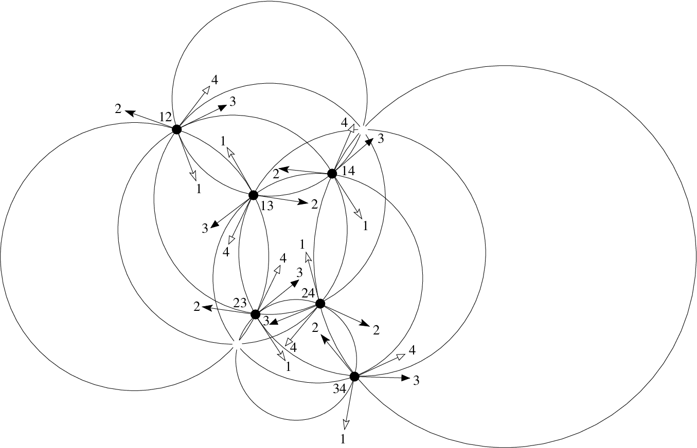
For completeness, it is remarked that the most general admissible orientation of the circles is obtained by simultaneously changing the orientation of a face of the octahedron and its three neighbours and then iterating this operation.
If we now demand that an oriented circle and its tangent vectors be of the same orientation then the following definition is natural:
Definition \thetheorem.
(Angles between circles) The angle made by two oriented circles and passing through a point of an octahedral point-circle configuration is that made by the two corresponding tangent vectors and at , viz
| (6) |
We are now in a position to define an analogue of Clifford’s classical configuration:
Definition \thetheorem.
(Generalized Clifford configurations) An octahedral point-circle configuration is termed a generalized Clifford configuration if the six points are equivalent in the sense that for any six pairs of corresponding oriented circles passing through the angle is independent of .
The following theorem demonstrates that the above definition is natural:
Theorem 3.1.
(Planar generalized Clifford configurations) Generalized Clifford configurations on the plane coincide with classical Clifford configurations.
Proof 3.2.
The Godt-Ziegenbein property (Godt 1896; Ziegenbein 1941) consists of the equivalence of the points of a classical Clifford configuration. Thus, in particular, the points of any given Clifford configuration are equivalent and hence the above definition of a generalized Clifford configuration is met. Conversely, let be the six points of a planar generalized Clifford configuration. If we set set aside the point , say, then it is evident that, due to the assumption of equivalence, may be reconstructed from the other five points . Indeed, since the four circles passing through are determined by these five points, the angles made by all pairs of circles are known so that, in turn, the remaining four circles are uniquely determined. On the other hand, the above five points also belong to a unique classical Clifford configuration as discussed in the previous section. The latter has the Godt-Ziegenbein property and hence coincides with the given generalized Clifford configuration.
4 Quaternions
It is well known that the group of conformal transformations in , consists of translations, rotations, scalings and inversions (Dubrovin et al. 1984). Accordingly, generalized Clifford configurations are objects of conformal geometry since circles are mapped to circles. In the current context, it is therefore natural to identify the four-dimensional Euclidean space with the algebra of quaternions (Koecher & Remmert 1991). Thus, we adopt the quaternionic representation
| (7) |
where the matrices are defined by
| (8) |
Then, the following properties and identities may be established.
Firstly, it is readily verified that
| (9) |
In particular, if, for non-vanishing quaterninons, we denote the corresponding unit vectors by
| (10) |
then
| (11) |
Secondly, Cayley’s theorem (Koecher & Remmert 1991) states that any element of the orthogonal group is represented by either
| (12) |
depending on whether is ‘proper’ () or ‘improper’ () respectively. Conversely, any quaternionic action of the above type corresponds to an orthogonal mapping . In particular, the operation
| (13) |
constitutes a reflection in the vector . Finally, the group of conformal transformations is generated by the orientation-preserving Möbius transformations (Ahlfors 1981)
| (14) |
and the particular reflection (conjugation)
| (15) |
5 Quaternionic cross- and multi-ratios
The relevance of multi-ratios in connection with classical Clifford configurations has been indicated in §2. It turns out that generalized Clifford configurations may also be described algebraically in terms of quaternionic multi-ratios. It is recalled that the cross-ratio of four points in is usually taken to be (Ahlfors 1981)
| (16) |
The cross-ratio is ‘real’, that is
| (17) |
if and only if the four points lie on a circle. The multi-ratio of six points may be defined as
| (18) |
or, alternatively,
| (19) |
In the scalar case, the ‘right-multi-ratio’ and the ‘left-multi-ratio’ are evidently identical. However, in the quaternionic case, the two multi-ratios are related by
| (20) |
This relation shows that the multi-ratio conditions
| (21) |
and
| (22) |
on six points coincide. Furthermore, it is readily seen that the Möbius transformations individually preserve the multi-ratio conditions (21) and
| (23) |
while (21) and (23) are mapped to each other by the conformal transformations which change the orientation. The geometric significance of this fact in the context of generalized Clifford configurations is discussed in the following section.
6 Existence and algebraic description of generalized Clifford configurations
It has been shown in §2 that planar generalized Clifford configurations are uniquely determined by five points. It turns out that the derivation of an analogous statement in the general case is the key to an algebraic description of generalized Clifford configurations. To this end, it is convenient to make a canonical choice of the tangent vectors to oriented circles. Thus, since four points are concyclic if and only if their cross-ratio is real, the function defined by
| (24) |
parametrizes the oriented circle which passes through as increases with . Differentiation and evaluation at then results in the tangent vector
| (25) |
at the point . The latter identity is merely a property of any three matrices and . Moreover, if two oriented circles and meet at the points and with associated tangent vectors and at then the vectors and given by (cf. (13))
| (26) |
are tangent to the circles and at and the orientation of the tangent vectors is preserved.
In order to proceed, we introduce a natural labelling of the points of an octahedral point-circle configuration and the vertices of its underlying octahedron. Thus, the six vertices of the octahedron are labelled by , in such a way that opposite vertices carry complementary indices and the corresponding points of the configuration are denoted by throughout the remainder of this paper.
Theorem 6.1.
(‘Uniqueness’) There exist at most two generalized Clifford configurations which share five points and the four associated circles.
Proof 6.2.
For convenience, we label the five common points by and regard the point(s) as unknown. Accordingly, only the four circles , passing through the point are known. The tangent vectors to these circles are linearly dependent and may be chosen to be
| (27) |
as indicated in figure 5. Here, the notation etc. has been adopted. In the generic case, any three of these four vectors span the three-dimensional tangent hyperplane to the hypersphere at defined by the five points . By virtue of the correspondence principle and the orientation convention, the orientation of the eight circles is now defined.
The vectors
| (28) |
are tangent to the circles and respectively at the point , while
| (29) |
constitutes a tangent vector to the circle at the point . Now, in order to determine the two remaining tangent vectors at the point , we make use of the assumption that, in particular, the points and are equivalent. Thus, the circle which passes through the points and gives rise to the relations
| (30) |
while the circle is associated with the additional relation
| (31) |
where . If the tangent vector to at the point is denoted by then the vector
| (32) |
is tangent to the circle at the point . Accordingly, the conditions (30) and (31) translate into
| (33) |
which may be written as
| (34) |
with the definition
| (35) |
The constraints (34) constitute a linear system for the unit vector . Hence, there are two cases to distinguish:
Case 1: If the tangent vectors span a two-dimensional plane then the five points necessarily lie on a 2-sphere (or a plane). On use of a conformal transformation, this 2-sphere may be mapped to a plane so that we are left with the consideration of generalized Clifford configurations in a three-dimensional Euclidean space subject to the five points being co-planar. If there exists a generalized Clifford configuration for which does not lie on the corresponding plane then reflection of in produces another generalized Clifford configuration. Furthermore, the classical Clifford configuration defined uniquely by the five points constitutes a third (planar) generalized Clifford configuration. Thus, the number of distinct generalized Clifford configurations sharing five co-planar points is odd.
On the other hand, it is readily seen that the rank of the linear system (34) is 2 since the tangent vectors are linearly dependent and hence there exist at most two solutions . Any specific choice of determines the tangent vector up to its magnitude. Moreover, since the angles between the vectors and the vector which is tangent to the circle passing through the points and are known and the four vectors must be linearly dependent, the direction of the tangent vector is uniquely determined. This, in turn, shows that the point is unique. Thus, there exist at most two generalized Clifford configurations. We therefore conclude that the above-mentioned classical Clifford configuration is the only generalized Clifford configuration under the current assumption.
Case 2: If the tangent vectors span a three-dimensional vector space then the tangent vectors are linearly independent without loss of generality. Accordingly, the rank of the linear system (34) is 3 and the corresponding two solutions are given by
| (36) |
It is noted that the above solutions are distinct since equality implies that and hence are linearly dependent. In fact, since the projections of and onto and coincide, the unit vectors and are related by reflection in the three-dimensional vector space spanned by . As in the previous case, any specific choice of now determines the point uniquely so that there exist at most two generalized Clifford configurations.
Remarkably, the above analysis implies that generalized Clifford configurations in three-dimensional Euclidean spaces or spheres are essentially two-dimensional.
Theorem 6.3.
Any generalized Clifford configuration in a three-dimensional Euclidean space or a three-dimensional sphere is either planar or confined to a two-dimensional sphere and may therefore be mapped to a classical Clifford configuration by means of a suitable conformal transformation.
Proof 6.4.
Since any generalized Clifford configuration in a three-dimensional hypersphere may be mapped via a conformal transformation to a generalized Clifford configuration in a three-dimensional subspace of , we may confine ourselves to the case of a generalized Clifford configuration in which we denote by and regard as being embedded in . As in the preceding proof, we consider the five points and set aside the point . If the tangent vectors span a two-dimensional plane then the generalized Clifford configuration is planar or confined to a 2-sphere as shown above. Hence, we may assume without loss of generality that . This implies, in turn, that the two solutions and of the linear system (34) are distinct and are related by reflection in . Hence, .
The key observation is now the following:
Theorem 6.5.
(Multi-ratio description of generalized Clifford configurations) The points of a generalized Clifford configuration are related by either
| (37) |
or
| (38) |
Conversely, any six points of an octahedral point-circle configuration which obey either of the multi-ratio conditions (37) or (38) constitute the points of a generalized Clifford configuration.
Before we prove the theorem, it is observed that the above multi-ratio conditions are representatives of two equivalence classes of multi-ratio conditions which may be imposed on an octahedral point-circle configuration. Specifically, let us consider an oriented hexagon with fixed ‘initial’ vertex formed by six edges of an octahedron with distinct vertices in such a way that any two adjacent edges of the hexagon belong to a triangular face of the octahedron (cf. figure 6) and impose the multi-ratio condition
| (39) |
on the points of an associated octahedral point-circle configuration. There exist such hexagons and in the planar case the associated multi-ratio conditions are equivalent. However, the situation is different in the (generic) quaternionic case.

Lemma 6.6.
Proof 6.7.
On the one hand, a typical permutation which leads to a non-trivial ordering of the arguments in the multi-ratio conditions is given by . The associated multi-ratio condition
| (40) |
may be brought into the form
| (41) |
The identities
| (42) |
then lead to
| (43) |
which, in turn, is the original multi-ratio condition (37).
On the other hand, composition of the subgroup of permutations with any ‘rotation by 90 degrees’ of the octahedron generates the remaining 24 discrete symmetries. For instance, the rotation produces the multi-ratio condition
| (44) |
which is, by definition, equivalent to
| (45) |
The latter is merely the tilde version of (40) and hence equivalent to the multi-ratio condition (38).
We are now in a position to prove theorem 6.5.
Proof 6.8.
(of theorem 6.5) By virtue of theorem 6.1 and the fact that either of the multi-ratio conditions (37) or (38) may be regarded as a definition of a point in terms of five arbitrary points, it remains to show that the multi-ratio conditions indeed give rise to generalized Clifford configurations. Thus, we here assume that the six points of an octahedral point-circle configuration are constrained by one of the multi-ratio conditions and choose the tangent vectors as in the proof of lemma 6.1. Accordingly, a set of corresponding tangent vectors of the correct orientation at the point is given by (cf. figure 5)
| (46) |
The expressions (35) and (36) for the quantities and suggest that one should consider the orientation- and angle-preserving mappings
| (47) |
Indeed, it is readily verified that
| (48) |
(cf. (28)) and a short calculation reveals that
| (49) |
Two conclusions may now be drawn from lemma 6.6. Firstly, the conditions (37) and (38) are equivalent to
| (50) |
and
| (51) |
respectively and hence it follows that
| (52) |
depending on whether (37) or (38) is assumed to hold. Thus, the points and are equivalent in the sense of definition 3 since
| (53) |
Secondly, since the points and are equivalent, the points and are equivalent for any permutation of the indices . Hence, all points are equivalent. This completes the proof.
We conclude this section with the remark that if a point of a generalized Clifford configuration which is not conformally equivalent to a classical Clifford configuration is inverted with respect to the hypersphere which passes through the other five points then another generalized Clifford configuration is obtained. Thus, theorem 6.5 implies the following corollary:
Corollary 6.9.
If two generalized Clifford configurations defined by
| (54) |
are not conformally equivalent to a classical Clifford configuration then the points and are related by inversion with respect to the (well-defined) hypersphere passing through the common points .
Interestingly, if one chooses the points in such a way that lies ‘at infinity’ then the above corollary implies that the point constitutes the centre of the hypersphere which passes through these five points.
7 The quaternionic discrete Schwarzian KP equation
In Konopelchenko & Schief (2002), it has been demonstrated that the multi-ratio condition (3) interpreted as a lattice equation is nothing but a Schwarzian version of the discrete Kadomtsev-Petviashvili (dKP) equation which constitutes a ‘master equation’ in the theory of integrable systems (Ablowitz & Segur 1981; Zakharov et al. 1980). Accordingly, the dSKP equation admits a geometric interpretation in terms of classical Clifford configurations. Here, we present an analogous construction of three-dimensional ‘Clifford lattices’ in a four-dimensional Euclidean space associated with the quaternionic multi-ratio condition. Due to the absence of any additional points of intersection of the circles belonging to a generic generalized Clifford configuration, not only is the quaternionic case more natural but it also includes the afore-mentioned scalar case.
We consider lattices of the combinatorics of a face-centred cubic (fcc) lattice in a four-dimensional Euclidean space, that is maps of the form
| (55) |

Any six points of which constitute the centres of the faces of a cube composed of eight adjacent elementary cubes of may be regarded as the vertices of an octahedron (cf. figure 7). In this way, the fcc lattice may be identified with the vertices of a collection of octahedra which meet at common edges. Accordingly, constitutes a set of points belonging to octahedral point-circle configurations. It is therefore natural to require that these point-circle configurations be of generalized Clifford type. In terms of the labelling (55), this implies that for any octahedron centred at with even, one of the multi-ratio conditions
| (56) |
and
| (57) |
obtains, where the arguments of have been suppressed and the notation
| (58) |
has been adopted. Two well-defined maps are obtained by demanding that the ‘same’ multi-ratio condition is imposed on all octahedra. Thus, we say that the map defines a Clifford lattice in if either (56) or (57) regarded as a lattice equation holds. It is noted that these two equations are essentially identical in the sense that if is a solution of (56) then is a solution of (57) and vice versa.
If the fcc lattice is mapped to a simple cubic lattice via the relabelling
| (59) |
defined by
| (60) |
then the lattice equation (56) assumes the standard form of the quaternionic reduction
| (61) |
of the integrable multi-component dSKP equation (Bogdanov & Konopelchenko 1998), wherein the subscripts on now refer to unit increments of the variables .
The conformal geometry of the qdSKP equation (61) and the associated (discrete) Schwarzian Davey-Stewartson II hierarchy has been discussed in detail in Konopelchenko & Schief (2005). Therein, it has been shown that any standard discrete isothermic surface (Bobenko & Pinkall 1996) may be extended via a translational symmetry to a three-dimensional lattice in such a manner that a (degenerate) Clifford lattice is obtained. In particular, Clifford lattices encapsulate discrete surfaces of constant mean curvature and discrete minimal surfaces. Thus, apart from its significance in connection with (generalized) Clifford configurations, the qdSKP equation also plays an important role in the area of integrable discrete differential geometry (Bobenko & Seiler 1999).
The geometric integrability of the qdSKP equation (61) may be shown by embedding generalized Clifford configurations in four-dimensional lattices of suitable combinatorics so that any three-dimensional ‘slice’ constitutes a generalized Clifford lattice. In the case of classical Clifford configurations, Desargues’ classical theorem (Pedoe 1970) turns out to be the key to the construction of a well-posed Cauchy problem for planar Clifford lattices. However, a reformulation of Desargues’ theorem in terms of angles is required in order to formulate a well-posed Cauchy problem for four-dimensional Clifford lattices in . In this manner, the standard Lax representation (Bogdanov & Konopelchenko 1998) and a Bäcklund transformation for the qdSKP equation may be derived geometrically. A detailed discussion of this topic goes beyond the scope of this paper and is consigned to a separate publication.
Ablowitz, M. J. & Segur, H. 1981 Solitons and the inverse scattering transform, Philadelphia: SIAM.
Ahlfors, L. V. 1981 Möbius transformations in several dimensions, Ordway Professorship Lectures in Mathematics, Univ. Minnesota.
Bobenko, A. I. & Pinkall, U. 1996 Discrete isothermic surfaces. J. reine angew. Math. 475, 187–208.
Bobenko, A. I. & Seiler, R. (eds) 1999 Discrete integrable geometry and physics, Oxford: Clarendon Press.
Bogdanov, L. V. & Konopelchenko, B. G. 1998 Analytic-bilinear approach to integrable hierarchies. II. Multicomponent KP and 2D Toda lattice hierarchies. J. Math. Phys. 39, 4701–4728.
Brannan, D. A., Esplen, M. F. & Gray, J. J. 1999 Geometry, Cambridge University Press.
Brown, L. M. 1954 A configuration of points and spheres in four-dimensional space. Proc. R. Soc. Edinb. A 64, 145–149.
Clifford, W. K. 1871 A synthetic proof of Miquel’s theorem. Oxford, Cambridge and Dublin Messenger of Math. 5, 124–141.
Cox, H. 1891 Application of Grassmann’s Ausdehnungslehre to properties of circles. Quart. J. Pure Appl. Math. 25, 1–71.
Coxeter, H. S. M. 1956 Review of Brown (1954). Math. Rev. 17, 886.
de Longechamps, G. 1877 Note de géometrie. Nouvelle Corresp. Mathèmat. 3, 306–312; 340–347.
Dorfman, I. Ya & Nijhoff, F. W. 1991 On a 2+1-dimensional version of the Krichever-Novikov equation. Phys. Lett. 157A, 107–112.
Dubrovin, B. A., Fomenko, A. T. & Novikov, S. P. 1984 Modern geometry – methods and applications. Part I. The geometry of surfaces, transformation groups, and fields, New York: Springer Verlag.
Godt, W. 1896 Ueber eine merkwürdige Kreisfigur. Math. Ann. 47, 564–572.
Grace, J. H. 1898 Circles, spheres and linear complexes. Trans. Camb. Phil. Soc. 16, 153–190.
Hirota, R. 1981 Discrete analogue of a generalized Toda equation. J. Phys. Soc. Japan 50, 3785–3791.
Koecher, M. & Remmert, R. 1991 Hamilton’s quaternions. In Numbers (ed. H.-D. Ebbinghaus, H. Hermes, F. Hirzebruch, M. Koecher, K. Mainzer, J. Neukirch, A. Prestel & R. Remmert). Graduate Text in Mathematics/Readings in Mathematics, no. 123, pp. 189–220, New York: Springer Verlag.
Konopelchenko, B. G. & Schief, W. K. 2002 Menelaus’ theorem, Clifford configurations and inversive geometry of the Schwarzian KP hierarchy. J. Phys. A: Math. Gen. 35, 6125–6144.
Konopelchenko B. G. & Schief, W. K. 2005 Conformal geometry of the (discrete) Schwarzian Davey-Stewartson II hierarchy. Glasgow Math. J. 47A, 121–131.
Longuet-Higgins, M. S. 1972 Clifford’s chain and its analogues in relation to the higher polytopes. Proc. R. Soc. Lond. A 330, 443–466.
Pedoe, D. 1970 A course of geometry, Cambridge University Press.
Zakharov, V. E., Manakov, S. V., Novikov, S. P. & Pitaevski, L. P. 1980 Soliton theory. The inverse problem method, Moscow: Nauka; 1984 New York: Plenum Press.
Ziegenbein, P. 1941 Konfigurationen in der Kreisgeometrie. J. reine angew. Math. 183, 9–24.