Department of Physics \principaladvisorDr. Andrew C. Doherty
Acknowledgements
This thesis is a consequence of direct and indirect contributions from various people, without whom I would not have gone this far. It is almost inevitable that I would miss some names in the following enumeration. For that matter, I would now declare that if you are in doubt, then yes, you must have been one of the contributors and I thank you for your help in one way or another. This is, of course, not an excuse for me to not express my appreciation explicitly and I shall attempt to do that in what follows.
The successful completion of my PhD candidature as well as this thesis would have been impossible, if not highly improbable without the help and guidance from my principal supervisor, Dr. Andrew C. Doherty. Andrew is always full of ideas and this means a lot to a junior researcher like me who sometimes lacks insight into the key issue of a problem. In particular, his physical intuition has enabled me to see the forest, instead of trees at various occasions. His comments on language usage have always been of great help too. On the other hand, I must also thank Andrew for his generous support in regard of me traveling overseas to attend conferences — these opportunities have, no doubt, greatly expanded my horizons. Finally, I owe Andrew a big thank you for going the extra miles to read through the earlier drafts of this thesis and giving me his valuable comments.
Many thanks to Guifré Vidal who has effectively acted as my associate supervisor, giving me his timely advice both in and out of Physics. This proved to be of upmost importance especially towards the end of my PhD candidature. Thanks also to Michael Nielsen, who has offered some critical comments on my research and who has always tried to made the quantum information science initiative in the University of Queensland a wonderful learning environment. His insistence on our active participation in seminars has undeniably done me a great favor in these years.
I am also thankful to my other present collaborators — Lluís Masanes, Ben Toner, Stephanie Wehner, Valerio Scarani — as well as past collaborators — Dagomir Kaszlikowski, Leong Chuan Kwek, Berthold-Georg Englert, Ajay Gopinathan and Choo Hiap Oh — for giving me the opportunity to learn from them. Among which, I am above all grateful to Dagomir Kaszlikowski and Leong Chuan Kwek for bringing me into this exciting field of quantum information science. Thanks also to Jing-Ling Chen, Shiang Yong Looi and Meng Khoon Tey for their helpful discussions.
The fellow PhD students sharing the same office as me are certainly not to be forgotten. I thank Eric Cavalcanti for enriching my philosophical understanding of nature, making this doctorate of philosophy a well-justified one. Of course, his never ending list of puzzles and paradoxes has also refreshed my ordinary research life from time to time. Chris Foster is definitely the most reliable mathematician, technician, and entertainer in Room 302. His trademark of trying to make sloppy calculations in Physics rigorous is both enlightening and inspiring. His help over these years, which often results in delaying his own research progress, is greatly appreciated. Next, I would like to thank Paulo Mendonça for always willing to listen to my complaints and sharing with me the unusual experience that he has been through. Thanks also to Paulo for proofreading an earlier draft of this thesis. Certainly, the random humor from Andy Ferris is much appreciated too.
I am also grateful to all of my other friends, especially those coming from the UQ Badminton Club. You guys have complemented my academic life in just the right way. Finally, I would also like to acknowledge the generous financial support from the International Postgraduate Research Scholarships (IPRS) and the University of Queensland Graduate School Scholarships (UQGSS).
List of Publications
Publications by the Candidate Relevant to the Thesis
-
Yeong-Cherng Liang and Andrew C. Doherty, Better Bell-inequality violation by collective measurements. Physical Review A 73, 052116 (2006)
-
Yeong-Cherng Liang and Andrew C. Doherty, Bounds on quantum correlations in Bell-inequality experiments. Physical Review A 75, 042103 (2007)
-
Lluís Masanes, Yeong-Cherng Liang and Andrew C. Doherty, All bipartite entangled states display some hidden nonlocality. Physical Review Letters 100, 090403 (2008)
-
Yeong-Cherng Liang, Lluís Masanes and Andrew C. Doherty, Convertibility between two-qubit states using stochastic local quantum operations assisted by classical communication. Physical Review A 77, 012332 (2008)
Additional Publications by the Candidate Relevant to the Thesis but not Forming Part of it
-
Andrew C. Doherty, Yeong-Cherng Liang, Stephanie Wehner, and Ben Toner, The quantum moment problem and bounds on entangled multi-prover games, Proceedings of the 23rd IEEE Conference on Computational Complexity, pp. 199–210 (eprint arXiv:0803.4373)
Abstract
It is one of the most remarkable features of quantum physics that measurements on spatially separated systems cannot always be described by a locally causal theory. In such a theory, the outcomes of local measurements are determined in advance solely by some unknown (or hidden) variables and the choice of local measurements. Correlations that are allowed within the framework of a locally causal theory are termed classical. Typically, the fact that quantum mechanics does not always result in classical correlations is revealed by the violation of Bell inequalities, which are constraints that have to be satisfied by any classical correlations. It has been known for a long time that entanglement is necessary to demonstrate nonclassical correlations, and hence a Bell inequality violation. However, since some entangled quantum states are known to admit explicit locally causal models, the exact role of entanglement in Bell inequality violation has remained obscure. This thesis provides both a comprehensive review on these issues as well as a report on new discoveries made to clarify the relationship between entanglement and Bell inequality violation. In particular, within the framework of a standard Bell experiment, i.e., a Bell inequality test that is directly performed on a single copy of a quantum state , we have derived two algorithms to determine, respectively, a lower bound and an upper bound on the strength of correlations that can offer for any given Bell inequality. Both of these algorithms make use convex optimization techniques in the form of a semidefinite program. By examples, we show that these algorithms can often be used in tandem, in conjunction with convexity arguments, to determine if a quantum state can offer nonclassical correlations and hence violates a given Bell inequality. On the other hand, since a standard Bell experiment typically involves measurements over many copies of the quantum systems, we have also investigated the possibility of enhancing the strength of nonclassical correlation by, instead, performing collective measurements on multiple copies of the quantum systems. Our findings show that even without postselection, such joint measurements may also lead to stronger nonclassical correlations, and hence a better Bell inequality violation. Meanwhile, previous studies have indicated that entangled state admitting locally causal models may still lead to observable nonclassical correlations if, prior to a standard Bell experiment, the state is subjected to some appropriate local preprocessing. This phenomenon of hidden nonlocality was discovered more than a decade ago, but to date, it is still not known if all entangled states can demonstrate nonclassical correlations through these more sophisticated Bell experiments. A key result in this thesis then consists of showing that for all bipartite entangled states, observable nonclassical correlations, in the form of a Bell-CHSH inequality violation, can indeed be derived if we allow both local preprocessing and the usage of shared ancillary state which by itself does not violate the Bell-CHSH inequality. This establishes a kind of equivalence between bipartite entanglement and states that cannot be simulated by classical correlations. In summary, for a standard Bell experiment where no local preprocessing on a quantum state is allowed, we have provided two algorithms that can be used in tandem to determine if can be simulated by a locally causal theory, whereas in the scenario where local preprocessing is allowed, we have demonstrated that bipartite entangled states are precisely those which cannot always be simulated classically.
List of Abbreviations
- aka
also known as
- lhs
left-hand-side
- rhs
right-hand-side
- BIV
Bell-inequality-violating
- CH
Clauser-Horne
- CHSH
Clauser-Horne-Shimony-Holt
- CGLMP
Collins-Gisin-Linden-Massar-Popescu
- CPM
completely positive map
- EPR
Einstein-Podolsky-Rosen
- GHZ
Greenberger-Horne-Zeilinger
- LB
lower bound
- LHV
local hidden variable
- LHVM
local hidden-variable model
- LHVT
local hidden-variable theory
- LMI
linear matrix inequality
- LOCC
local quantum operations assisted by classical communication
- MEMS
maximally entangled mixed states
- NBIV
non-Bell-inequality-violating
- NSD
negative semidefinite
- POVM
positive-operator-valued measure
- PPT
positive-partial-transposed
- PSD
positive semidefinite
- QCQP
quadratically-constrained quadratic program
- SLO
stochastic local quantum operations without communication
- SLOCC
stochastic local quantum operations assisted by classical communication
- SDP
semidefinite program
- SOS
sum of squares
- UB
upper bound
Chapter 1 Introduction
The advent of Quantum Mechanics is undeniably an important milestone in our attempt to understand Nature. On the one hand, quantum mechanics is well-known for giving very accurate predictions for microscopic phenomena, whereas on the other, it has also given some counter-intuitive predictions which seem nonsensical from a classical view point. Among the many intriguing features of quantum mechanics is entanglement [18, 19] which, loosely speaking, refers to the situation whereby two or more spatially separated physical systems are so strongly correlated that it may become impossible to independently describe the physical state of the individual systems. The significance of entanglement can be seen, for example, in the following quotation by Schrödinger [18],
“…I would not call that one but rather the characteristic trait of quantum mechanics, the one that enforces its entire departure from classical lines of thought. By the interaction the two representatives have become entangled. …”
The astonishing features of entanglement were first brought to our attention in 1935 via the influential work by Einstein, Podolsky and Rosen (henceforth abbreviated as EPR) [20], and subsequently popularized by Schrödinger’s thought experiment on an innocent cat [19].11 1 See also the English translation by Trimmer [21]. Specifically, in Ref. [20], EPR considered a pair of physical systems that are so strongly correlated that it becomes possible to predict, with certainty, some properties of the distant physical system by simply performing measurements on the local one. Exploiting such bizarre correlations offered by entanglement, EPR eventually came to the conclusion that the quantum mechanical predictions of physical reality is incomplete [20], just as statistical mechanics is incomplete within the framework of classical mechanics [22, 23].
For a long time after that, discussions arising out of EPR’s paper remained largely a philosophical debate. However, as Bell [5, 24] showed in the 1960s, the possibility of completing the quantum mechanical predictions in the way that EPR sought does lead to experimentally falsifiable consequences. In particular, by considering a variant of EPR’s argument due to Bohm [25], Bell [5] showed that quantum mechanical predictions on spatially separated systems cannot always be described by a locally causal theory. In such a theory, the outcomes of measurements are determined in advance merely by the choice of local measurements and some local hidden variable — which can be seen as information exchanged between the subsystems during their common past. Bell has thus ruled out the possibility of providing a locally causal description for all quantum phenomena — a brutal fact of life that is now succinctly called Bell’s theorem.
Typically, the incompatibility between a locally causal description and the quantum mechanical prediction for a quantum state due to some choice of observables is revealed by the violation of Bell inequalities, which are statistical constraints that have to be satisfied by all locally causal theories. Since the early 1980s, there have been numerous experiments reporting Bell inequality violation in various physical systems (see, for example, Refs. [26, 27, 28]). While it is clear that entanglement is necessary to demonstrate a Bell inequality violation, by generalizing the notion of entanglement to mixed states, Werner [29] has found that not all entangled states can violate a Bell inequality (see also Refs. [30, 31, 32, 33]). In fact, it is not even known if all multipartite pure entangled states are Bell-inequality-violating [34, 35, 36, 37]. This state of affairs has inspired some to consider more general, nonstandard Bell experiments to reveal the bizarre correlations hidden in quantum states. In this regard, it was later shown by Popescu [38] and others [39, 40] that if a Bell experiment is preceded with appropriate local preprocessing, then a non-Bell-inequality-violating quantum state may become Bell-inequality-violating — a phenomenon that is now known as hidden nonlocality.
In recent years, the rising field of quantum information processing has also brought a resurgent interest in the study of Bell inequality violation. The pioneering work in this regard is due to Ekert [41], who showed that Bell inequality violation can be used to guarantee the security of a class of quantum key distribution protocols. Since then, a great deal of work has been carried out in this regard (see, for example, Refs. [42, 43, 44, 45, 46] and references therein). In fact, recently, it has even been argued in Refs. [45, 46] that Bell-inequality violation is necessary to guarantee the security of some entanglement-based quantum key distribution protocols. On the other hand, Bell inequality violation was also found to be relevant in other quantum information processing tasks, such as reduction of communication complexity [47, 48, 49]. In the context of quantum teleportation [50], Horodeckiet al. [51] have shown that all two-qubit states violating a Bell inequality are useful for teleportation; Popescu, however, has shown that some two-qubit states not violating the same Bell inequality are also useful for teleportation [52]. Of course, given that quantum entanglement is an essential ingredient in many quantum information processing protocols [43], it is by no means accidental that a verification of entanglement through Bell inequality violation is carried out daily in many laboratories in the world.
Given the importance of Bell inequality violation, both from a foundational point of view and its relevance in quantum information processing, it is perhaps surprising that there are still many open problems related to the study of Bell inequality violation [53]. In particular, little is known as to which quantum states can violate a Bell inequality, both in a standard scenario and in a nonstandard scenario which also involves local preprocessing. Even when a quantum state is known to violate a Bell inequality, the extent of violation is in most cases not well-quantified. On a related note, the maximal violation that quantum mechanics allows for a given Bell inequality is also not well-studied beyond some simple cases [54, 55, 56, 57, 58, 17].
The main goal of this thesis to clarify the relationship between Bell inequality violation and quantum entanglement by determining the set of quantum states that can give rise to nonclassical behavior. The structure of this thesis is as follows. From Chapter 2 – Chapter 4, we will provide a comprehensive review of the theoretical background of the thesis. Specifically, Chapter 2 deals with some of the important concepts relevant to local causality and the key historical developments leading to Bell’s theorem. Then in Chapter 3, we will give a more technical introduction to the set of classical correlations,22 2 This is the set of correlations allowed by a locally causal theory. which includes a formal introduction to the idea of a tight [59, 60], or facet-inducing Bell inequality [61]. Some of the well-known tight Bell inequalities will also be reviewed. After that, we will proceed to the quantum regime in Chapter 4 and introduce the notion of quantum correlation following Ref. [62]. Some well-known examples of entangled quantum states admitting a locally causal description will then be reviewed.
Most of our new research findings can be found in the second part of the thesis, from Chapter 5 – Chapter 7, while the rest are left in the appendices. In Chapter 5, we will present new findings in relation to the problem of determining if a given quantum state can violate some fixed but arbitrary Bell inequality via a standard Bell experiment. In particular, using convex optimization techniques [63] in the form of a semidefinite program [64], we have derived two algorithms to determine, respectively, a lower bound and an upper bound on the strength of correlation that a quantum state can display in some given Bell experiments. These tools are also applied in Chapter 6 where we will look at some of the best known Bell inequality violations displayed by entangled states. Given that in practice, a Bell experiment involves measurements on many copies of the same quantum systems, we also investigated the possibility of getting a better Bell inequality violation by using collective measurements without postselection; this is the other subject of discussion in Chapter 6. Next, in Chapter 7, we will look into the possibility of deriving nonclassical correlations from all entangled quantum states. In particular, with the aid of an ancilla state which does not violate the Bell-CHSH inequality, we will provide a protocol to demonstrate a Bell-CHSH inequality violation coming from all bipartite entangled states. This provides a positive answer to the long-standing question of whether all bipartite entangled states can lead to some kind of observable nonclassical correlations. Finally, we will conclude with a summary of key results and some possibilities for future research in Chapter 8.
Chapter 2 Bell’s Theorem and Tests of Local Causality
In this chapter, we will give a brief historical review of the study of local causality in quantum mechanics. We will begin with the incompleteness arguments presented by Einstein, Podolsky and Rosen [20], and see how that had led to the celebrated discovery by Bell [5, 24]. After that, some of the key developments towards an experimental test of local causality will also be reviewed.
2.1 Bell’s Theorem
2.1.1 The Einstein-Podolsky-Rosen Incompleteness Arguments
Quantum mechanics, as is well-known, only gives predictions, via the wavefunction or state vector, on the probabilities of obtaining a certain outcome in an experiment (see, for example, Ref. [65, 66]). Moreover, according to Bohr’s complementarity [67, 68, 69], physical quantities described by two non-commuting observables in the theory are incompatible in that a complete knowledge of one precludes any knowledge of the other. This scenario is clearly in discord with the classical intuition that objective properties of physical systems exist independent of measurements.
Among those who were unsatisfied with Bohr’s complementarity were Einstein, Podolsky and Rosen (EPR) who together put forward, in their 1935 paper [20], the argument that any complete physical theory must be such that
“every element of the physical reality must have a counterpart in the physical theory.”
A sufficient condition for the reality of a physical quantity that they have provided is as follows [20]:
“if without in any way disturbing a system, we can predict with certainty (i.e., with probability equal to unity) the value of a physical quantity, then there exists an element of physical reality corresponding to this physical quantity.”
According to these criteria, Bohr’s complementarity implies at least one of the followings, namely, (1) quantum mechanics is not a complete theory, or (2) the two physical quantities corresponding to non-commuting observables cannot have simultaneous reality. Moreover, by considering local measurements on two physical systems that have interacted in the past but are separated at the time of measurements, EPR came to the conclusion that if (1) is false, so is (2).
As an example, EPR considered a two-particle system described by the wavefunction
| (2.1) |
where and are, respectively, the coordinates
attached to the two particles, is some arbitrary constant
and is the eigenvalue of the momentum operator for the
first particle. It is not difficult to see that for both
position and momentum measurements on the two particles, the
outcomes derived are always perfectly correlated. In
particular, if Alice and Bob are, respectively, at the
receiving ends of the two particles, their measurement outcomes
on these particles will read:
| Measurement | Alice | Bob |
|---|---|---|
| Momentum | ||
| Position |
Therefore, according to the criterion set up by EPR, should be measured on the first particle, the momentum of the second particle is an element of physical reality; whereas if is measured on the first particle, the position of the second particle is an element of physical reality. Moreover [20],
since at the time of measurement the particles no longer interact, no real change can take place in the second system in consequence of anything that may be done to the first system.
Hence, by EPR’s criterion of reality, both and of the second particle, though corresponding to noncommuting observables in the theory, can have simultaneous reality, corresponding to the negation of (2). Since negation of (1) also led to the negation of (2), while at least one of (1) and (2) has to be true, EPR concluded that the quantum mechanical description of physical reality given by wavefunction is incomplete. Furthermore, at the very end of the paper [20], EPR optimistically expressed their belief that a theory that provides a complete description of physical reality is possible.
2.1.2 Completeness and Hidden-Variable Theory
Although no explicit proposal was given by EPR, it was commonly inferred from their arguments and the success of statistical mechanics that a complete description of physical reality can be attained if unknown (hidden) variables are supplemented to the wavefunction description of physical reality (see, for example Ref. [23] and references therein). Indeed, not known to EPR and many other founding fathers of quantum mechanics, towards the end of 1920s, de Broglie constructed a hidden-variable theory that is capable of explaining the quantum interference phenomena while retaining the corpuscular feature of individual particles [70, 71].
Despite that, the idea of completing the description given by quantum mechanics with additional variables has received much criticism over the years (see for example Ref. [24] and references therein). Among them, von Neumann’s proof (pp. 305, Ref. [72]) of the impossibility of (noncontextual) hidden variables probably provided peace in mind to most of those who were against the proposal. The proof given by von Neumann in Ref. [72] has, nevertheless, imposed unnecessary restrictions on the unknown variables [24]. In fact, this was made blatant after Bohm rediscovered the hidden-variable theory [73, 74] first formulated by de Broglie [70, 71].
Nonetheless, Bohmian mechanics or the pilot-wave model, as the de Broglie-Bohm hidden-variable theory is currently known, was dismissed by many physicists because of the explicit “nonlocal” flavor in the theory. Ironically, it was precisely the discovery of this controversial theory that led Bell [75, 24] to consider, instead, the possibility of a local hidden-variable theory and hence his important discovery in 1964 [5].
For Einstein, he was firmly convinced that (pp 672, [22])
“…within the framework of future physics, quantum theory takes an analogous position as statistical mechanics takes within the framework of classical mechanics.”
Adhering to the same philosophy, Bell’s consideration of a hidden-variable theory [5] is such that an average over some unknown ensemble labeled by the hidden-variable gives rise to the statistical behavior of quantum mechanical prediction. As Bell emphasized, the variables are hidden because they are not known to exist; they are not even accessible in principle, otherwise “quantum mechanics would be observably inadequate” [24, 76].
Clearly, not all hidden-variable theories are welcome in the physics community [24]. For instance, in the hidden-variable theory formulated by de Broglie and Bohm [73, 74], the trajectory of one particle may depend explicitly on the trajectory as well as the wavefunction of other particles that it has interacted with in the past, regardless of their spatial separation. This “nonlocal” feature of the theory is in apparent contradiction with the well-established intuition of causality that we have learned from special theory of relativity. Therefore, following EPR’s flavor, Bell considered hidden-variable theories that are local such that, in Bell’s words [5]:
“…the result of measurement on one system be unaffected by operations on a distant system with which it has interacted in the past …”
In later years, a theory that satisfies Bell’s notion of locality, or more specifically
“The direct causes (and effects) of events are near by, and even the indirect causes (and effects) are no further away than permitted by the velocity of light.”
is said to be locally causal [77]. Hereafter, we will use the term local hidden-variable theory (henceforth abbreviated as LHVT) and the term locally causal theory interchangeably.11 1 The other terminology that is also commonly found in the literature is local realistic theory; this is however not as universally accepted, see e.g. Ref. [78]. As we shall see below, Bell’s greatest contribution came in by showing that quantum mechanics is not a locally causal theory [5, 24].
2.1.3 Quantum Mechanics is not a Locally Causal Theory
To illustrate this remarkable fact of life, Bell [5] has chosen to work within the framework first presented by Bohm (Sec 15 – 19, Chap 22, Ref. [25]) concerning the spin degrees of freedom of two spin- particles, which is the analog of EPR’s scenario for discrete variable quantum systems.22 2 Incidentally, the experimental situation described in the original EPR paper [20] can indeed be explained within the framework of a locally casual theory [79]. In this version of EPR’s argument, pairs of spin- particles are prepared in the spin singlet state
| (2.2) |
where and are correspondingly the spin up and spin down state of one of the particles with respect to some spatial direction33 3 Since the spin singlet state is isotropic, the actual space quantization axis is immaterial. (likewise for and ). After that, particles in each pair are separated and sent to two experimenters (hereafter always denoted by Alice and Bob), who can subsequently perform spin measurements along some (arbitrary) direction and , respectively, on these particles (c.f. Figure 2.1). Now, recall from quantum mechanics that the expectation value of such measurements reads
| (2.3) |
where
| (2.4) | |||
| (2.5) |
is the unit vector pointing in the positive direction (likewise for and ) and
| (2.6) |
are the Pauli matrices (here, we adopt the convention that , ). Thus, if , the measurement outcomes on both sides must be perfectly (anti-) correlated, i.e., if Alice’s measurement outcome reads “”, Bob’s measurement outcome must read “”. Since this is true for other pair of and such that , hence, by virtue of EPR’s original argument, one can conclude that the “spin” along any direction for both of these particles must be “element of physical reality”.
Now, let us follow Ref. [5] and denote by any additional parameters carried by the particles that could provide a complete specification for these physical realities. Physically, we can think of as information that is exchanged between the particles during the preparation procedure but which is not completely encoded in the state vector . As remarked in Ref. [5], the exact nature of is irrelevant, it could refer to a single or a set of random variables, or even a set of functions and it could take on continuous as well as discrete values. If we denote by and , respectively, the measurement outcome observed at Alice’s and Bob’s side, then by Bell’s requirement of locality, we must have as a function of and but not ; likewise for . Furthermore, the measurement outcome at each side is completely determined by these parameters such that [5]
| (2.7) |
here, we adopt the convention that measurement outcomes “” and “” are assigned the value “” and “” respectively. Let us now define the correlation function as
| (2.8) |
where is the space of hidden-variable and is some normalized probability density such that
| (2.9) |
Physically, the correlation function, Eq. (2.8), is just the average of the product of local measurement outcomes over an ensemble of physical systems characterized by some distribution of hidden-variable, . It then follows that a necessary condition for getting a complete description of the above-mentioned physical realities using local hidden-variable is that for all and
| (2.10) |
for some choice of , and some choice of that is independent of and . As we shall see below, Eq. (2.10) cannot be made true in general. Nonetheless, it is interesting to note that Bell has constructed a specific local hidden-variable model 44 4 Throughout this thesis, we will use the term local hidden-variable model to refer to, say, a set of rules, that can be used to reproduce some set of experimental statistics; it is less general than a LHVT, which is supposed to be able to reproduce all experimental statistics generated by quantum mechanics. (henceforth abbreviated as LHVM) that makes it true for the case when [5].
To show that Eq. (2.10) cannot be made true for all possible choices of measurement parameters, Bell introduced another unit vector and considered the following combination of correlation functions:
From triangle inequality, Eq. (2.7) and Eq. (2.9), it follows that
| (2.11) |
When , it follows from Eq. (2.3) that . Therefore, Bell further assumed in Ref. [5] that if the measurement parameters chosen by both observers coincide, the outcomes of measurement, as determined by the hidden variables are also perfectly correlated:
| (2.12) |
With this assumption, the above inequality becomes
| (2.13) |
which gives the very first inequality that has to be satisfied by any LHVT in the literature [5]. In the spirit of Bell’s original work, let us introduce the following definition for a Bell inequality.55 5 It is worth noting that among the physics community, the term Bell inequality, or Bell-type inequality has sometimes been used to refer to inequality that arises out of an entanglement witness. To appreciate the distinction between these two kinds of inequalities, see, for example, Refs. [80, 81].
Definition 1.
A Bell inequality is an inequality derived from the assumptions of a general local hidden-variable theory.
In Ref. [5], Bell subsequently gave a formal proof, based on Eq. (2.13), that cannot equal or even be approximated arbitrarily closely by . However, to illustrate the point that quantum mechanics also gives rise to predictions not allowed by any LHVT, it suffices to show that for some choice of measurement parameters, the quantum mechanical version of Eq. (2.13), namely,
| (2.14) |
is violated. To this end, let us assume that all the spin measurements are performed on the plane and that points along the direction of the positive -axis, i.e., . Then, for the choice of
| (2.15) |
it can be easily verified using Eq. (2.3) that quantum mechanics predicts 1/2 for the lhs of inequality (2.14), thereby demonstrating that quantum mechanical prediction is, in general, incompatible with that given by any LHVT, c.f. Eq. (2.13).
The above finding gives rise to the following important theorem first derived by Bell [5]:
Theorem 2.
No local hidden-variable theory can reproduce all quantum mechanical predictions. Equivalently, quantum mechanics is not a locally causal theory.
2.2 Towards an Experimental Test of Local Causality
2.2.1 Bell-Clauser-Horne-Shimony-Holt Inequality
The inequality (2.13) derived by Bell [5] has clearly demonstrated that some quantum mechanical predictions, in the ideal scenario, cannot be reproduced by any LHVT. However, the assumption of perfect correlation, c.f. Eq. (2.12), or equivalently,
| (2.16) |
for is too strong to be justified in any realistic experimental scenario. The Bell inequality (2.13) was therefore not readily subjected to any experimental test. A few years later, in 1969, a resolution was provided by Clauser, Horne, Shimony and Holt (henceforth abbreviated as CHSH) who, instead of Eq. (2.16), assumed that for some [6]
| (2.17) |
where . To conform with the prediction given by quantum mechanics, one expects that for spin measurement on the singlet state and when is (approximately) aligned with , is close to but not exactly equal to zero.
Now, let’s take this imperfect correlation into account by dividing the space of hidden-variable into such that
| (2.18) |
Then, it follows from Eq. (2.8), Eq. (2.9), Eq. (2.17) and Eq. (2.18) that
| (2.19) |
Instead of inequality (2.13), inequality (2.11) now leads to
which, together with Eq. (2.17), becomes
| (2.20) |
This is the famous Bell-CHSH inequality that was first derived in Ref. [6]. It is interesting to note that a few years later [76], Bell gave an alternative derivation66 6 Strictly, the inequality that was later derived by Bell reads: (2.21) but as we shall see below, we can essentially treat it as the same inequality as that given by Eq. (2.20). of inequality (2.20) by respectively replacing Eq. (2.7) and Eq. (2.8) with
| (2.22) |
and
| (2.23) |
Here, Bell tried to be more general (as compared with his approach in Ref. [5]) by assuming that the measurement apparatuses could also contain hidden-variable that could influence the experimental results. In the above expressions, is thus used to denote an average over the hidden-variable associated with Alice’s apparatus when it is set to perform measurements parameterized by ; similarly for .
At this stage, it is worth making a few other remarks. Firstly, in contrast with Bell’s first inequality, Eq. (2.13), that was developed for spin measurements on the singlet state, the Bell-CHSH inequality is also relevant to other physical states as well as other physical systems. In fact, it is applicable, as a constraint imposed by LHVTs, to any experimental statistics involving two spatially separated subsystems and where two dichotomic77 7 A dichotomic measurement is one that yields one out of two possible outcomes. measurements — each giving outcomes labeled by — can be performed on each of the subsystems. Essentially, this means that in the more general experimental framework, the parameters etc. are merely labels to distinguish the different measurements that Alice and Bob may perform on the subsystem in their possession.
As a result, and for the convenience of subsequent discussion, let us introduce the following notation for the correlation function associated with Alice measuring the observable and Bob measuring the observable , i.e.,
| (2.24) |
where the outcomes of local measurements and are now functions of the hidden variable and, respectively, the local observables and . In particular, if we now make the following associations between the measurement parameters and the local observables :
| (2.25) |
it is clear that both inequality (2.20) and inequality (2.21) imply the following inequality:
| (2.26) |
Evidently, if this is a valid constraint that has to be satisfied by any LHVT, so is any other obtained by relabeling the local observers (“Alice” “Bob”), local measurement settings (, ) and/or outcomes (). For example, if we instead make the associations , and relabel all the outcomes at Alice’s site by and vice versa, then we will arrive at
| (2.27) |
which is clearly different from inequality (2.26). Nonetheless, the difference between these inequalities, which is due to a different choice of labels, is physically irrelevant. After all, when testing a set of experimental data against a Bell inequality, the choice of these labels is completely arbitrary. As such, let us define the equivalence class of Bell inequalities as follows [59, 60].
Definition 3.
A Bell inequality is equivalent to another if and only if one can be obtained from the other by relabeling the local observers, local measurement settings and/or measurement outcomes.
Under this definition, it is straightforward to see that apart from inequality (2.27), inequality (2.26) is also equivalent to 6 other inequalities. Hereafter, when there is no risk of confusion, we will refer to inequality (2.26) as the Bell-CHSH inequality and to the entire class of 8 inequalities that are equivalent to inequality (2.26) as the Bell-CHSH inequalities. In relation to inequality (2.20), it is also not difficult to see that this inequality is violated if and only if (at least) one of the Bell-CHSH inequalities is violated; likewise for inequality (2.21).
As a last remark, we note that the Bell-CHSH inequality is an example of what is now called a (Bell) correlation inequality — a Bell inequality that only involves linear combination of correlation functions. Clearly, a correlation function, which can be determined experimentally by averaging over the product of the outcome of local observables, is not the only quantity that is derivable from a given set of experimental data; the relative frequency of experimental outcomes, in the limit of large sample size, gives a good approximation to the probability of obtaining that particular outcome. In the next section, we will look at an example of the other prototype of (linear) Bell inequalities, namely, one that involves a linear combination of joint and marginal probabilities of experimental outcomes.
2.2.2 Bell-Clauser-Horne Inequality
The earlier work by CHSH is no doubt a big step towards an experimental test for the feasibility of locally casual theories. However, due to imperfect detection and other realistic experimental concerns, the Bell-CHSH inequality (2.26) can only be put into a real experimental test when supplemented with an auxiliary assumption on the ensemble of detected particles [6, 82]. Specifically, in the context of polarization measurement on photons, the original assumption made by CHSH is that if a pair of photons emerges from the respective polarizers located at Alice’s and Bob’s side, the probability of their joint detection is independent of the orientation of the polarizers.
A few years later, work by Clauser and Horne (hereafter abbreviated as CH) demonstrated that without an auxiliary assumption, neither the experiment carried out by Freedman and Clauser [83] nor any similar ones with improved detector efficiency can give a definitive test of locally causal theories [7]. To remedy the problem, CH derived, in the same paper [7], another Bell inequality and showed that when supplemented with a considerably weaker no enhancement assumption, the results obtained by Freedman and Clauser are indeed incompatible with LHVTs [7].

The scenario that CH considered is a familiar one, namely, one that involves ensembles of two particles being sent to Alice and Bob respectively. Under the control of each experimenter is an analyzer with an adjustable parameter (denoted by and respectively) and a detector. At each run of the experiment, let us denote by the state of the two-particle system and the probability that for this two-particle state, a count is triggered at both detectors conditioned on Alice setting her analyzer to and Bob setting his to ; the marginal probabilities of detecting a particle and are similarly defined. In these terminologies, the no enhancement assumption states that for a given state , the probability of detecting a particle with the analyzer removed is greater than or equal to the probability of detecting a particle when the analyzer is in place.
Now, note that for a given (normalized) probability density characterizing the ensemble of states emitted, the observed relative frequencies should correspond to
| (2.28) |
It is worth noting that as it is, the above formulation could very well be applied to quantum mechanical prediction, with the wavefunction playing the role of . As with the correlation function, Eq. (2.8), the condition of local causality comes in by demanding that the probability of joint detection factorizes [7], i.e.,
| (2.29) |
From the definition of probabilities, it follows that
| (2.30) |
where and are some other choice of parameters for the analyzers. Together, Eq. (2.29) and Eq. (2.30) imply that [7]
for each given . After averaging over the ensemble space , one arrives at
| (2.31) |
which is the Bell-CH inequality — the very first Bell inequality for probabilities derived in the literature. Notice that to arrive at the lower limit of inequality (2.31), we also have to assume that the probability density is normalized, Eq. (2.9).
Let us now make a few other remarks concerning inequality (2.31). To begin with, we note that although the inequality was derived by considering a one-output-channel analyzer that is followed by a single detector, it could very well be applied to measurement devices equipped with two (or more) detectors, thereby giving rise to two (or more) possible outcomes.88 8 Strictly, there are three possible outcomes when there are two detectors, with the other possible outcome corresponding to no detection. In particular, for the specific case of two possible outcomes, which we will label as “”, the same analysis allows us to arrive at the inequality [7]
| (2.32a) | |||
| and | |||
| (2.32b) | |||
where each measurement outcome and can be “” and is now the probability of Alice observing outcome and Bob observing outcome conditioned on her performing the measurement and him performing the measurement; the marginal probabilities and are analogously defined. Notice that the four inequalities (2.32b) are actually equivalent to inequalities (2.32a) and can be obtained from the latter, for example, via the identity .
Let us also remark that the set of 8 inequalities given in Eq. (2.32) are symmetrical with respect to swapping & and have taken into account all possible ways of labeling of the outcomes. Nevertheless, additional equivalent inequalities, such as
| (2.33) |
can still be obtained by relabeling the local measurement settings. Hereafter, unless stated otherwise, the term Bell-CH inequality would refer to Eq. (2.32a) with only two possible outcomes.
In relation to the Bell-CHSH inequality, we recall that the correlation function defined in Eq. (2.24) can actually be rewritten as99 9 To this end, we are identifying the measurement at Alice’s site as a measurement of while the measurement at Bob’s site as a measurement of .
| (2.34) |
i.e., the average value of the product of observables or
| (2.35) |
which is the difference between the probability of observing the same outcomes at the two sides and the probability of observing different outcomes at the two sides. Thus, by adding the two inequalities in Eq. (2.32a) with and subtracting them from the two inequalities with , one arrives at the Bell-CHSH inequality in the form of Eq. (2.26). Conversely, if there are only two possible outcomes such that
| (2.36) |
then all the four Bell-CH inequalities given in Eq. (2.32a) can also be obtained from the Bell-CHSH inequalities via Eq. (2.34) or Eq. (2.35). Hence, when seen as a set of constraints imposed by LHVTs on two particles, where each of them is subjected to two alternative dichotomic measurements, the Bell-CH inequalities are entirely equivalent to the Bell-CHSH inequalities [7].
2.2.3 Experimental Progress
Since the late 1960s, many experiments have been carried out, via the Bell-CH and Bell-CHSH inequalities, to probe the adequacy of locally causal theories. An account of the early attempts prior to the 1980s can be found in the excellent review by Clauser and Shimony [82]. These early results, however, were not compelling enough to close the debate due to the various possible loopholes in experiments [84].
Among which, the communication loophole survived happily till the influential experiment performed by Aspect and coworkers in 1982 using time-varying analyzers [85]. Since then, many have considered the impossibility of a LHVT verified, even though some still think otherwise (see for example [86, 87, 88, 89, 90] and references therein). As of now, the experiment that most convincingly evades the communication loophole was carried out by Weihs and collaborators in 1998 [91]. The equally notorious detection loophole has also been closed quite recently by Rowe and coworkers [27]. A single experiment that closes both these loopholes at once is, nevertheless, still being sought [26, 92]. In this regard, it is worth noting that some other loopholes such as those considered in Refs. [93, 94] exist, but they are generally considered less compelling. For further information on recent Bell experiments, see the review by Genovese [95].
Chapter 3 Classical Correlations and Bell Inequalities
In the last chapter, we have seen two important examples of Bell inequalities that were developed in the hope of realizing a convincing test of local causality. Bell inequalities, nevertheless, can also be understood from a completely different perspective. Specifically, in this chapter, we will see that in the space of probability vectors, which we will call the space of correlations, the tight Bell inequalities correspond to hyperplanes that together form the boundaries of the convex set of classical correlations.11 1 Although our treatment focuses (almost) exclusively on probability vectors, it should be clear that one can just as well consider a space of correlations that is defined in terms of various correlation functions, as in Eq. (2.24). In that case, a (tight) Bell correlation inequality similarly defines a closed halfspace where the convex set of classical correlations resides. Froissart is apparently the pioneer of such a geometrical approach to Bell inequalities [96]. Not too long after that, this approach was discovered independently by Garg and Mermin [97]. A few years later, a general study along the same lines was also carried out by Pitowsky [62, 98]. A great advantage of this geometrical approach is that it can be easily generalized to more complicated experimental scenarios and hence, allows more complicated Bell inequalities to be derived in a systematic manner.
3.1 Classical Correlations and Probabilities
Before we move on to the more general scenario, let us first go through the following example of a hypothetical Bell experiment to gain some intuition. In particular, let us consider an experimental scenario where the Bell-CHSH inequality, or equivalently the two-outcome Bell-CH inequality, is applicable (Figure 2.1). Now, let us imagine that the experimental data collected (Table 3.1) — including those not explicitly shown in the table — satisfy the following joint probabilities
| (3.1a) | ||||
| (3.1b) | ||||
| (3.1c) | ||||
| (3.1d) | ||||
| and marginal probabilities | ||||
| (3.1e) | ||||
| (3.1f) | ||||
Evidently, we can collect all the 16 joint probabilities together and think of them as the components of a probability vector living in a 16-dimensional space. Let us now make the following definitions in relation to such a probability vector.
Definition 4.
A probability vector is said to be classical if it can be generated from some local hidden-variable model.
Hereafter, we will also loosely refer to a probability vector as a correlation. This can be justified by noting that from the components of a probability vector, we can learn the extent to which measurement outcomes between subsystems and are correlated. For example, if and involved in the experiment are totally uncorrelated, we will expect that all the joint probabilities factorize and equal to the product of the corresponding marginal probabilities, i.e.,
| (3.2) |
Moreover, all experimental statistics that could be of interest, such as the correlation function for given measurement settings, as well as other higher order moments can be computed according to the standard procedures.
| 1 | 1 | 1 | ||
| 2 | 1 | 1 | ||
| 3 | 1 | 1 | ||
| 4 | 1 | 1 | ||
| 5 | -1 | 1 | ||
| ⋮ | ⋮ | ⋮ | ⋮ | ⋮ |
| 1000 | 1 | -1 |
| 1001 | -1 | -1 | ||
| 1002 | 1 | 1 | ||
| 1003 | 1 | 1 | ||
| 1004 | 1 | 1 | ||
| 1005 | -1 | 1 | ||
| ⋮ | ⋮ | ⋮ | ⋮ | ⋮ |
| 1 | -1 |
Now, let us again look at the set of experimental data presented in Table 3.1. If there exists a LHVM that can reproduce this set of data, we will be able to fill in the blanks corresponding to unperformed measurement results such that all the joint and marginal probabilities are preserved. Therefore, if the unfilled entries in the table can be filled up in such a way that respects all the probabilities listed in Eq. (3.1), we will have got a LHVM that reproduces all the experimental statistics, and hence correlations derivable from Table 3.1. An example of how this can be done is shown in Table 3.2. In this case, we can see as an index for the local hidden-variable that is associated with each run of the experiment. Then, in each run , once the choice of local measurement is decided, the outcome of the measurement can be read off directly from the table (regardless of the other entries listed in the same row of the table).
| 1 | 1 | (1) | 1 | (1) |
| 2 | 1 | (-1) | (1) | 1 |
| 3 | (1) | 1 | 1 | (1) |
| 4 | 1 | (-1) | 1 | (-1) |
| 5 | (1) | -1 | (1) | 1 |
| ⋮ | ⋮ | ⋮ | ⋮ | ⋮ |
| 1000 | 1 | (-1) | (1) | -1 |
| 1001 | (1) | -1 | (1) | -1 |
| 1002 | 1 | (1) | 1 | (-1) |
| 1003 | (1) | 1 | (1) | 1 |
| 1004 | 1 | (1) | 1 | (-1) |
| 1005 | (1) | -1 | 1 | (1) |
| ⋮ | ⋮ | ⋮ | ⋮ | ⋮ |
| (1) | 1 | (1) | -1 |
That a LHVM can be constructed for the data presented in Table. 3.1 is not incidental. Simple calculations using Eq. (2.32) and Eq. (3.1) show that none of the Bell-CH inequalities is violated by the experimental data presented in Table. 3.1. Evidently, no-violation of the Bell-CH inequality is a necessary condition for the existence of a LHVM for the given experimental data. Nevertheless, as was first shown by Fine in 1982 [99], fulfillment of all the Bell-CH inequalities is also sufficient to guarantee the existence of a LHVM, provided that the experimental data only involves two dichotomic measurements performed by two observers [100, 101, 102]. Hence, in an experimental scenario involving only two observers and two dichotomic measurements per site, a complete characterization of classical correlations can be obtained solely using the Bell-CH inequalities. What about experiments involving more observers, more local measurements per site, or more outcomes per measurement? These are the questions that we will discuss in the following sections.
3.2 Geometrical Structure of the Set of Classical Correlations
3.2.1 The Spaces of Correlations
For the subsequent discussion, let us consider a more general scenario whereby a source — characterized by some physical state — distributes pairs of physical systems to Alice and Bob, and where each of them can perform (on the subsystems that they receive), respectively, and alternative measurements that would each generates and distinct outcomes.22 2 Of course, one can be more general than this and allows each measurement to have different number of possible outcomes. Nevertheless, for brevity, we shall be contented with a discussion on the case where all local measurements performed by Alice yield the same number of possible outcomes (likewise for Bob). For now, we will restrict our attention to this bipartite scenario, but most of the following arguments can be modified easily to cater for the multipartite scenario. In view of the forthcoming discussion, let us also introduce the vectors
| (3.3) |
for, respectively, a compact description of the number of local measurement settings and the number of possible outcomes for each local measurement. As with the previous section, the experimental statistics in such a scenario can be summarized as a probability vector where (if one prefers to work in the space of correlations that is defined only in terms of full correlation functions , then we will be working in a space of dimension — Sec. 3.3.2). The components of the probability vectors are the joint probabilities .33 3 One can, instead, work in a space of probabilities with dimension such that each probability vector also has the marginal probabilities and as components. However, this is not necessary, as the marginal probabilities are not independent from the joint probabilities. We will refer to this real vector space as the space of correlations, denoted by . Clearly, for our purpose, not all of the coordinates in are independent. For instance, given a particular choice of Alice’s and Bob’s measurement, there must be an outcome at Alice’s as well as Bob’s site.44 4 For the purpose of present discussion, one could treat the possibility of no-detection as one of the possible outcomes. Normalization of probability therefore requires:
| (3.4) |
where we have labeled the outcomes registered at Alice’s site as (likewise at Bob’s site). Moreover, adhering to the principles of relativity, we shall be contented with correlations that do not allow faster-than-light signaling. These are correlations that respect the following equalities [103]:
| (3.5) |
In words, this means that the marginal probability of Alice observing local measurement outcome , conditioned on her measuring , i.e., is independent of the choice of measurement made by the spatially separated observer Bob; likewise for . This is now commonly known as the no-signaling condition (see, for example, Refs. [104, 105]), which was originally termed the relativistic causality condition in Ref. [103].
By a simple counting argument, one can show that after taking into account all of these constraints, there are effectively only [60]
| (3.6) |
independent entries in the probability vector, which can be taken to be all but one of the marginal probabilities for each , likewise for , plus of the joint probabilities for each combination of and . Hence, we are essentially only interested in a subspace of the set of probability vectors that is of dimension .
3.2.2 The Convex Set of Classical Correlations
Now, let us take a closer look at the set of classical correlations associated with the experimental scenario described above. Hereafter, we will denote this set by (analogously, we will denote the set of classical correlations defined in the space of correlation functions as ). From Eq. (2.28) and Eq. (2.29), it follows that a classical probability vector is one whose entries satisfy
| (3.7) |
for some choice of and , and some probability density . For any two classical probability vectors and , any convex combination of them gives rise to a probability vector
| (3.8) |
that is also classical. This is because the resulting probability vector can be realized via a LHVM which consists of implementing the LHVM associated with and stochastically. Specifically, by tossing a biased coin with probability of getting heads and probability of getting tails, the probability vector can be realized by implementing the LHVM associated with whenever the outcome of the toss is heads, and the LHVM associated with whenever the outcome of the toss is tails. Therefore, the set of classical probability vectors is convex.
A natural question that follows is: what are the extreme points55 5 An extreme point of a convex set is a point in the set which cannot be expressed as a nontrivial convex combination of two or more different points in the set [106, 107]. of this set? With some thought, it is not difficult to see that probability vectors such that the joint probability factorizes, i.e.,
| (3.9a) | |||
| and for which the marginal probabilities are either 0 or 1, i.e., | |||
| (3.9b) | |||
are extreme points of [60]. These are probability vectors corresponding to deterministic LHVMs. Physically, each of these probability vectors corresponds to a scenario where the experimental outcomes for given local measurement settings are deterministic; once the local measurement setting is chosen, one and only one of the local detectors will ever click.66 6 In the context of and where measurement outcomes are bounded between and the extreme points correspond to those whereby . Conversely, it is also not difficult to see from Eq. (3.7) and Eq. (3.9) that any other classical probability vectors can be written as a nontrivial convex combination of these extremal probability vectors. In other words, a probability vector is an extreme point of if and only if it satisfies Eq. (3.9).
Given that the physical scenario corresponding to an extreme point of is such that the local measurement settings determine the local measurement outcome with certainty, we might as well label each of these extreme points by two sets of indices and that are, respectively, associated with the measurement outcomes observed by Alice and Bob [108] (Figure 3.1). Specifically, let us denote by an extreme point of , Alice’s measurement outcome conditioned on her measuring and Bob’s measurement outcome conditioned on him measuring . Then the two sets of indices where and where will completely characterize in the sense that its component reads [108]
| (3.10) |

For finite number of local measurement settings and measurement outcomes, i.e.,
it is possible to enumerate all of these extreme points by going through all legitimate boolean values of the local probabilities. In total, there are thus
| (3.11) |
extremal classical probability vectors, corresponding to extremal deterministic LHVMs. Hereafter, we will also refer to the extreme points of a convex polytope as its vertices, denoted as . The fact that there are only a finite number of extreme points in the (convex) set of classical correlations immediately implies that is a convex polytope [106, 107], which was first called the correlation polytope by Pitowsky [98]. Notice that the dimension of the correlation polytope, i.e., the dimension of its affine hull77 7 An affine combination of a set of points is a linear combination of , i.e., such that . The affine hull of is the union of all affine combinations of . is .
3.2.3 Correlation Polytope and Bell Inequalities
A well-established fact about a convex polytope is that it can equivalently be represented by the intersection of a finite family of closed halfspaces [106, 107]. As is well-known, a closed halfspace in can be represented by an inequality that is linear in the coordinates. Let us denote by the inequality that is associated with the “”-th halfspace “bounding” the polytope , i.e.,
| (3.12) |
then the boundary associated with this halfspace is the hyperplane
| (3.13) |
where is an arbitrary vector in the space of correlations, is a vector defining the “direction” of the hyperplane involved, represents the Euclidean inner product between the two vectors, and is some constant related to the offset of the hyperplane from the origin.
By definition, a classical probability vector is a member of and hence must satisfy inequality (3.12), i.e.,
| (3.14) |
The inequality (3.12) is therefore a valid constraint that has to be satisfied by all classical probability vectors. In other words, it is a Bell inequality. It is straightforward to see that any conic combination88 8 A conic combination of points is a non-negative linear combination of the points. of such inequalities will also give rise to another inequality that has to be satisfied by all . There is thus no unique family of inequalities defining a given correlation polytope . In principle, one can even write down an infinite family of Bell inequalities, each associated with a closed halfspace (and hence hyperplane), which has to be satisfied by all . In this regard, it is worth noting that the smallest family of such closed halfspaces consists of those whose boundaries are the affine hull of the facets99 9 The intersection of a polytope with a supporting hyperplane gives rise to a face of the polytope. If the dimension of a polytope is , then a face of dimension is known as a facet of the polytope. of (pp 31, [106]). In other words, Bell inequalities that are associated with this smallest family of halfspaces are characterized by and such that the solution set to each of the corresponding equalities
| (3.15) |
is nonempty and whose affine dimension equals . For definiteness, we will refer to them as tight Bell inequalities [59, 60], or equivalently facet-inducing Bell inequalities [61]. It is worth noting that the coefficients associated with these tight Bell inequalities, i.e., , when properly normalized, also define a convex polytope that is dual to the correlation polytope. Moreover, a probability vector is classical if and only if it satisfies this minimal set of Bell inequalities defining .1010 10 See, for example Definition 2.10 and Theorem 2.15 of Ref. [107].
For the convenience of subsequent discussion, let us note that the linearity of inequality (3.12) also allows us to write the functional form of a generic Bell inequality, c.f. Eq. (3.13), in the following tensorial form
| (3.16) |
where
| (3.17) |
is a component of the probability vector and is the corresponding component of the vector of coefficients . Notice that the sums over outcomes are restricted in that when , there is no sum over and when , there is no sum over ; in these special cases, we shall write
| (3.18) |
We can then write these coefficients in a compact manner via the following matrix
| (3.19) |
where each of the boldfaced entries in the above matrix is a block matrix of appropriate dimension. For example, in the above matrix is the following matrix
| (3.20) |
whereas and are, respectively, column vector and row vector of length and .1111 11 The length of these vectors as well as the dimension of each block matrix can be traced back to the discussion around Eq. (3.5). Consequently, for a two-outcome Bell inequality (e.g. the Bell-CH inequality), or a Bell correlation inequality, we will collapse each block matrix and write it as a single number. It is then expedient to write a Bell inequality explicitly as
| (3.21) |
but compactly as
| (3.22) |
where is the corresponding matrix of coefficients, Eq. (3.19) – Eq. (3.20), associated with the specific Bell inequality.
As an example, let us look at the simplest nontrivial scenario where and . In this case, it is known for a long time [99, 62, 109, 60] that the only class of nontrivial1212 12 The other tight Bell inequalities are trivial in the sense that they either require probabilities to be non-negative or not larger than unity. tight Bell inequalities are the Bell-CH inequalities listed in (2.32a) and their equivalents. In this case, we have1313 13 Hereafter, we will drop the arguments of for brevity of notation.
| (3.23) |
Making use of the matrix representation introduced above, we will write this class of inequalities as [60]
| (3.24) |
where for ease of reading, we will always replace each null entry in a matrix by a single dot.
A great advantage of this matrix representation is that a Bell inequality that only differs from another in its label of measurement settings can be obtained from (the matrix representation of) the other by applying an appropriate permutation to the rows and/or columns of blocks in the associated matrix of coefficients, c.f. Eq. (3.19). Similarly, two Bell inequalities that differ from another only in their label of measurement outcomes for a particular local measurement setting can be obtained from one another by applying appropriate permutation to the rows and/or columns within the entire row/column of blocks of matrix of coefficients, c.f. Eq. (3.20). And finally, two Bell inequalities that only differ in their label of observers, e.g. “Alice”“Bob”, can be obtained from one another by transposing their respective matrix of coefficients (see Appendix B.1.1 for examples). With this compact notation, the stage is now set for us to look into Bell inequalities that arise in the more complicated experimental scenarios.
3.3 The Zoo of Bell Inequalities
To date, a zoo of Bell inequalities is available in the literature. In particular, a handful of these were constructed in the 1980s [110, 111, 112, 113, 102, 97, 114] primarily to investigate if Bell inequality violation would vanish in one of the plausible classical limits. Some of these early attempts, however, suffered by their rather ad hoc construction of (non-tight) Bell inequalities. In what follows, we will review, via the characterization of various classical correlation polytopes , some of the more well-known (tight) Bell inequalities beyond Bell-CH and Bell-CHSH that can be, or have been constructed using the geometrical approach presented above.
For bipartite Bell inequalities, that is, Bell inequalities involving only two parties, our discussion will be carried out primarily for Bell inequalities for probabilities, as this is where most of the work was done [109, 60, 14]. On the contrary, most of the work for multipartite Bell inequalities were carried out in the context of Bell correlation inequalities, in particular those involving only the full correlation functions.1414 14 A full correlation function, as opposed to a restricted correlation function, for an -party Bell experiment is a correlation function that takes the local observables at all the sites as arguments [115] (see the discussion at pp. 3.38 for more details).
3.3.1 Other Bipartite Bell Inequalities for Probabilities
3.3.1.1 Two Outcomes
Now, let us focus on bipartite Bell inequalities for probabilities involving only dichotomic observables, i.e., . For scenarios involving more than two measurements on one side, but not on the other, i.e., or with , Collins and Gisin have shown in Ref. [60] that there are no new tight Bell inequalities. In other words, all facets of the correlation polytope (equivalently ) either correspond to the trivial requirement of probabilities being positive, or to a Bell-CH type inequality involving only two out of the possible measurements. An example of such an inequality would be [60]
| (3.25) |
in which case only statistics of Bob’s first and local measurement are involved in the above inequality.
In the case when each party is allowed to perform three alternative measurements, i.e., for the correlation polytope , a complete list of 684 facets was first obtained by Pitowsky and Svozil in Ref. [109]. Among these, Collins and Gisin [60] have found that there are 36 positive probability facets, 72 Bell-CH-type facets while the remaining facets are associated with inequalities that are equivalent to1515 15 The analogous analysis for Bell correlation inequalities with has also been carried out independently by Śliwa [116] (see also [96]).
| (3.26) |
Equivalently, in the notation of Eq. (3.17), inequality can be written more explicitly as:
| (3.27) |
which is understood to hold true for arbitrary but fixed choice of and .
Here, we again see that a lower dimensional Bell inequality, namely, the Bell-CH inequality occurring as a facet of a more complicated correlation polytope. As was shown by Pironio [117], this is actually a generic feature of tight Bell inequalities for probabilities1616 16 See Aviset al. [58] for the analogous proof for Bell correlation inequalities., i.e., when lifted to a more complicated experimental scenario, say, involving more local measurement settings and/or outcomes and/or number of parties, the lower dimensional Bell inequality will still serve as a tight Bell inequality in the higher dimensional space. Since a direct enumeration of all tight Bell inequalities is computationally intensive and may not be feasible in practice, this property of tight Bell inequalities will enable us to find out, at least, a partial list of facets in the higher dimensional correlation polytope [117].
For example, for the correlation polytope , even though a complete characterization of tight Bell inequalities for probabilities is not known, we do know from Pironio’s result [117] that all the tight inequalities derived from, say, will also serve as tight inequalities in the higher-dimensional space. This lower dimensional case has been fully characterized in Ref. [60] and the correlation polytope is known to made up of from five different classes of facets.
For , however, it is known that there are also other classes of tight Bell inequalities. For example, Collins and Gisin [60] have shown that a generalization of , namely,
| (3.28) |
is also a tight Bell inequality. By brute force, Itoet al. [14] have found two other tight Bell inequalities for this experimental scenario:
| (3.29) |
and by the method of triangular elimination [61], they have also found at least one other tight Bell inequality:
| (3.30) |
which they have labeled as “A5”. Very recently, a partial list of 26 inequivalent facet-inducing inequalities for was presented in Ref. [118].
Beyond this, a systematic characterization of all the tight Bell inequalities with more local measurements seems formidable. However, we do know that both and are members of a broader class of Bell inequalities, called by Collins and Gisin [60]. It is worth noting that this class of inequalities is asymmetric with respect to swapping Alice and Bob. In particular, for , the inequality admits the following compact representation [60, 61]:1717 17 Note that for the specific case of and , Eq. (3.31) is related to, respectively, Eq. (3.26) and Eq. (3.28) by a transposition, which corresponds to swapping the label “Alice” “Bob”. The current form of Eq. (3.31), as opposed to Eq. (3.26) and Eq. (3.28), looks closer to the original form presented in Refs. [60, 61].
| (3.31) |
For , Collins and Gisin computationally verified that
each is a tight Bell inequality, and for general
, the tightness of these inequalities has also been proven
very recently by Avis and Ito [119]. Apart
from this, Aviset al. [61] have also obtained
a huge number of tight Bell inequalities by applying the method
of triangular elimination to a list of tight inequalities for
the so-called cut polytope. On top of inequality
(3.30), the explicit form of some of these
inequalities with can also be found in
Ref. [14, 120].
3.3.1.2 More than Two Outcomes
The set of classical correlations involving greater number of measurement outcomes is apparently not as well known. In particular, investigation carried out by Collins and Gisin [60] suggests that for , all facets of the correlation polytope (equivalently ) are either of the Bell-CH-type or the trivial type that requires non-negativity of probabilities. For , it was shown by Masanes [59] that there is only one other class of tight Bell inequalities, which was discovered independently by Collinset al. [121] and Kaslikowskiet al. [122]. Following Ref. [60], we will write this inequality as
| (3.32) |
where and are, respectively, column vector of ones and zeros with length 2,
| (3.33) |
In Ref. [60], the inequality (3.32) was actually presented as a special case of a class of inequalities — which Collins and Gisin labeled as — that holds for arbitrary . Specifically, for , it takes the form of
| (3.34) |
where inequalities for higher values of involve the obvious modifications on individual blocks. For general , we can write in the following functional form:
| (3.35) |
This class of inequalities is believed [60] to be equivalent to the more well-known -outcome Collins-Gisin-Linden-Massar-Popescu (henceforth abbreviated as CGLMP) inequality [121], which admits the following functional form:1818 18 Here, we have swapped and (i.e., Bob’s first and second measurement settings) and followed Ref. [59] by grouping terms for the same setting together. Moreover, we have also shifted the constant “2” to the lhs of the inequality.
| (3.36) |
where expression such as in the above inequality is understood to be evaluated modulo . A proof of their equivalence is, however, not available in the literature. In Appendix B.1.1, we have provided this missing proof. The tightness of the CGLMP inequality, and hence was proven by Masanes in Ref. [59]. They therefore correspond to facets of for arbitrary .
Finally, we note that a family of (tight) Bell inequalities – the inequality — involving more than two measurements per site, and more than two outcomes per measurement has also been presented in Ref. [60]. However, the inequality is only known to correspond to facets of with for some relatively small values of and .
3.3.2 Other Bipartite Correlation Inequalities
Thus far, we have focused on the analysis of correlation polytopes living in the space of probability vectors and looked at the corresponding tight Bell inequalities bounding these polytopes. Now, let us turn our attention to the space of correlations defined in terms of correlation functions – denoted by — for an experimental scenario involving only two parties performing and dichotomic1919 19 Strictly, many of the subsequent discussion will still hold true even if we have more outcomes in the experiments, provided that all measurement outcomes are bounded between “” and “1”. measurements, and whose measurement outcomes are labeled by . Specifically, in this bipartite scenario, is a space of dimension , which can be labeled by the following coordinates [96, 58]
| (3.37) |
where the restricted correlation functions [115] are defined as
| (3.38) |
More often than not, however, we are only interested in the (sub)space of correlations that is defined solely in terms of the full correlation functions . We shall denote this subspace by . Note that it is a subspace of dimension . As with , the set of classical correlations in () is a convex polytope which we shall denote by ().
A well-known fact in relation to these polytopes is that the two polytopes and are actually isomorphic (see for example [58]). Therefore, any tight Bell inequality defining can also be mapped to a tight correlation inequality defining via Eq. (2.34) and Eq. (3.38). Nevertheless, for the purpose of performing this mapping, it is more convenient to make use of an equivalent form of Eq. (2.34),
| (3.39) |
For instance, in the simplest scenario of , one obtains the Bell-CHSH inequality from the Bell-CH inequality via Eq. (3.39). Similarly, by applying Eq. (3.38) and Eq. (3.39) to , Eq. (3.27), one can obtain the following correlation inequality [116, 58]
| (3.40) |
Note, nonetheless, that as opposed to the Bell-CHSH inequality, inequality (3.40) does not live in the subspace of full correlations , i.e., it is not a facet-inducing inequality for . In fact, recent work by Aviset al. [58] has demonstrated that for with , the Bell-CHSH inequalities and the trivial inequalities2020 20 In relation to Eq. (3.39) and Eq. (3.38), these trivial inequalities are in one-to-one correspondence with the trivial requirement of probabilities being non-negative and less than or equal to one.
| (3.41) |
for all and all , are the only tight correlation inequalities defining .
On the contrary, when four alternative measurements are allowed at each site, Gisin has constructed the following Bell correlation inequalities [53]
| (3.42) |
| (3.43) |
where the entry in each matrix is the coefficient associated with the full correlation function . These inequalities are tight. Together with the trivial inequalities (3.41) and the Bell-CHSH inequality, they form a complete set of tight correlation inequalities defining [58].
As a last remark, we note that the correlation inequality has been generalized to an arbitrary even number of measurement settings. Moreover, they can also be seen as a correlation inequality that is valid for arbitrary number of measurement outcomes if instead of Eq. (2.34) or Eq. (3.39), which are only for two-outcome Bell experiments, the full correlation function , Eq. (2.24), is interpreted as the difference between the probability of observing the same outcomes at the two sites and the probability of observing different outcomes at the two sites, as it was done in Eq. (2.35) [53].
3.3.3 Multipartite Bell Inequalities
In sharp contrast with the study of bipartite Bell inequalities — where most developments were carried out in the context of probability vectors — the multipartite analog was primarily developed in the context of correlation functions, and in particular the full correlation functions. The pioneering work in this regard was initiated by Mermin [123] who, in turn, was inspired by the results presented by Greenberger, Horne and Zeilinger (henceforth abbreviated as GHZ) on a demonstration of incompatibility between local causality and quantum mechanical prediction without resorting to any inequalities [124, 125] .
In his seminal work, Mermin [123] investigated a scenario involving parties and where each of them can perform two dichotomic measurements. Starting from the assumption of a general LHVM, Mermin constructed a Bell correlation inequality which involves only -partite full correlation functions; his inequality therefore defines a closed halfspace in where resides (here, there are indices in both the superscript2121 21 We are generalizing the notation introduced in Sec. 3.3.1 such that indices in the subscript (sequentially) indicate the number of possible measurements at each site and indices in the superscript indicate the number of possible outcomes per measurement at each site. and subscript). This work was further developed by Roy and Singh [126], Ardehali [127], and eventually by Belinskiǐ and Klyskho [128, 129] whereby the current form of Mermin inequality (also commonly known as Mermin-Ardehali-Belinskiǐ-Klyskho, or in short, MABK inequality) was culminated.2222 22 The inequality developed by Roy and Singh [126] is actually equivalent to the current form of Mermin’s inequality developed by Belinskiǐ and Klyskho [128, 129].
An interesting feature of the present form of Mermin’s inequality is that all inequalities involving parties can be obtained from the Bell-CHSH inequality in a recursive manner. To see that, let us now denote by the outcome of measurement when the observer chooses to measure the dichotomic observable. As a classical variable,2323 23 That is, a variable that can be defined using local hidden-variable. can be defined independently for each and each . Thus, in each run of the experiment, the expression
| (3.44) |
must either end up as or , since either or . Averaging this expression over many runs of the experiment, we see that the average value of must be less than or equal to 1, since each term in the average is at most 1. This is essentially a statement of the Bell-CHSH inequality given in Eq. (2.26).
To obtain the -partite Mermin’s inequality, we now follow Ref. [130] and define
| (3.45) |
where is the same expression as except that all the and are interchanged. By going through the same reasoning as before, it is not difficult to see that the average value of must be bounded above by 1, i.e.,
| (3.46) |
where here, refers to the expectation value of . It is also not difficult to see from Eq. (3.45) that is an expression that is linear in all the local variable , therefore by generalizing the notation introduced in Eq. (3.16), we can write
| (3.47) |
for some specific . Now, we can write the entire class of Mermin inequalities in a form that is closer to inequality (2.26), i.e.,
| (3.48) |
where is the -party correlation function defined analogous to Eq. (2.24).
As is now well-known, Mermin inequalities are not the only class of -partite Bell correlation inequalities. In fact, a complete2424 24 Complete, in the sense that a vector of full correlation functions is classical if and only if it satisfies all of these inequalities. set of Bell correlation inequalities involving only the full correlation functions has been obtained independently by Werner & Wolf [115] and Żukowski & Brukner [131] (the complete set of inequalities for was also obtained by Weinfurter and Żukowski in Ref. [132]). All these inequalities are uniquely characterized by the tensor , which can be written as [115]
| (3.49) |
where is a binary function that takes an -bit-vector (with components ) as argument. There are altogether of such functions, each of them gives rise to a unique tensor which, in turn, defines a Bell correlation inequality via Eq. (3.48). These inequalities are tight [115, 131], and therefore are facet inducing for the correlation polytope of -partite correlation functions . It happens that is actually a -dimensional hyperoctahedron [115], and hence the complete set of inequalities is equivalent to a single nonlinear inequality [115, 131].
More recently, by generalizing the work of Wu and Zong on [133], Laskowski and coworkers [134] have come up with a systematic way to generate a huge class of tight Bell correlation inequalities for . In particular, explicit forms of these facet-inducing inequalities for and can be found in Ref. [134]. A first step towards the complete characterization of facets for a more symmetrical experimental scenario, namely, was carried out in Ref. [135] by Żuwkoski. Apparently, a complete characterization for this experimental scenario has subsequently been achieved in Ref. [136]. Based on these findings, the explicit form of a tight correlation inequality for has very recently been derived and presented in Ref. [137].
Finally, we note that at present, only one facet-inducing inequality for is known, and is presented in the form of a coincidence Bell inequality [138]. Other multipartite Bell inequalities, such as those involving restricted correlation functions [139, 140, 141] or in the form of probability inequality [37] can also be found in the literature. Their tightness, however, is not well studied.
3.4 Conclusion
In this chapter, we have looked at the set of classical correlations, i.e., correlations (either in the form of probability vector or a vector of correlation functions) that are describable within the framework of LHVTs and how it is related to the zoo of Bell inequalities that one can find in the literature. Equipped with a solid understanding of the set of classical correlations, we will next investigate what quantum mechanics has to offer, both in terms of classical correlations and correlations that cannot be accounted for using any locally causal theory.
Chapter 4 Quantum Correlations and Locally Causal Quantum States
In the last chapter, we have looked at the set of classical correlations and the characterization of its boundaries in terms of Bell inequalities. Now, in this chapter, we will move on to study the set of quantum correlations and see how they are related to the set of classical correlations. Some well-known examples of quantum states admitting locally causal description will also be reviewed.
4.1 Introduction
In a nutshell, quantum correlations are simply points in the space of correlations, c.f. Sec. 3.2.1, that are realizable by quantum mechanics through some choice of quantum states and some local measurement operators. Ironically, despite the statistical nature of quantum predictions, there was no known study on this specific aspect of quantum predictions prior to the seminal work by Bell in 1964 [5].
After that, it seems to have taken another 16 years before the first quantitative study on the set of quantum correlations was carried out by Tsirelson11 1 Incidentally, in response to a question raised by A. M. Vershik (see pp. 884 of Ref. [142]). [143]. In his work [143], Tsirelson showed that the set of quantum correlations in is also bounded by some very similar linear inequalities like its classical partner. However, these linear inequalities (often known as the Tsirelson inequalities) are, in general, not sufficient to distinguish a correlation that is realizable by quantum mechanics from one that is not. In fact, it took a few more years before Tsirelson came up with a set of necessary and sufficient conditions — in terms of inequalities that are non-linear in the correlation functions — for the realizability of a point in using quantum mechanics [144, 145].
Meanwhile, a general study on the structure of the set of quantum correlations beyond the simplest scenario of was taken up by Pitowsky [146]. In fact, it was in Ref. [146] that the convexity of this set and its relationship with the set of classical correlations were, for the first time, formally established (see also Ref. [62]).
From Bell’s theorem [5], we have learned that there are quantum correlations that fall outside the classical correlation polytope. A characterization of quantum states that can give rise to such nonclassical correlations is, nevertheless, still lacking. The seminal work by Werner [29] has established that entanglement between spatially separated subsystems is a necessary condition to establish nonclassical correlation. Nonetheless, in the same article [29], Werner also provided an example of an entangled state which does not violate any Bell inequalities if the source is directly subjected to local, projective measurements without any preprocessing. In fact, there are now a few known examples of entangled quantum states which admit an explicit LHVM [29, 31, 32, 33].
In this chapter, we will start off, in Sec. 4.2, by reviewing some well-known facts about the set of quantum correlations. In the same section, we will also specify what we mean by a standard Bell experiment, a key notion that is used in this, as well as the subsequent chapters. After that, in Sec. 4.3, we will review some of the well-known examples of quantum states admitting either a partial, or a full LHVM for projective or generalized measurements given by positive-operator-valued measures (POVM).
4.2 Quantum Correlations
Consider again the set of two-party correlations that respects the relativistic causality condition, . In analogy with the idea of a classical probability vector introduced in Chapter 3, we will now define a quantum probability vector as follows.22 2 The definition is given for probability vectors considered in a bipartite correlation experiment and where correlations are expressed in terms of probability vectors. Nonetheless, it should be clear as to how this definition can be generalized to the multipartite scenario, or the space of correlations defined in terms of correlation functions.
Definition 5.
A probability vector in is said to be a quantum probability vector if there exists a bipartite quantum state acting on , i.e., , and some (local) POVM elements , , i.e., operators satisfying
| (4.1a) | |||
| (4.1b) | |||
such that the components of the probability vector satisfy
| (4.2a) | |||
| (4.2b) | |||
where and .
Note that in the above definition of a quantum probability vector , the dimension of the Hilbert spaces is not fixed a priori. In other words, the dimension of the Hilbert spaces involved may vary depending on the given probability vector. As with a classical probability vector, we shall also refer to a quantum probability vector, loosely, as a quantum correlation. Moreover, the set of quantum correlations will be denoted by .
Physically, a quantum probability vector is one whose components can be realized via what we shall call a standard Bell experiment.33 3 In the literature, the term standard Bell experiment has been used in various different contexts. In particular, it is commonly used to refer to a Bell experiment that involves measurements of two-dichotomic observables per site (i.e., ). When there are only two parties involved in the experiment, this reduces to an experiment that tests against the Bell-CHSH/ Bell-CH inequality. Here, we are using this term in the same sense as that used in Ref. [147], which distinguishes it from nonstandard Bell experiment that typically involves (either active or passive) preprocessing prior to an actual Bell test.
Definition 6.
A standard Bell experiment (in relation to ) on a source characterized by some quantum state is one whereby the source distributes pairs of physical systems to Alice and Bob, and where each of them can perform (on each physical system that they receive), respectively, and alternative measurements that would each generate and distinct outcomes.
Here, we have implicitly assumed that at the receiving ends, the composite systems that Alice and Bob receive are still well characterized by the same physical state and this is the assumption that we will make whenever we deal with a standard Bell experiment. With this assumption, then via a standard Bell experiment, the sets of local POVM elements , and the (bipartite) quantum state give rise to a quantum correlation via Eq. (4.2). As such, we will also say that , together with these POVM elements form a quantum strategy that realizes .
Of course, at a more general level, one can also imagine a scenario where Alice and Bob choose to perform local measurements on copies of the quantum systems at a time; this is the scenario of performing a standard Bell experiment on . Alternatively, one could also imagine that while the source is well characterized by , Alice and Bob may choose to perform some local preprocessing on which effectively transforms it to some other state prior to a standard Bell experiment. Loosely, we shall say that these are nonstandard Bell experiments on , since the source is still well characterized by . However, these and other scenarios which do not fit within the framework of a standard Bell experiment on will be the topics of future discussion in Chapter 6 and Chapter 7.
4.2.1 General Structure of the Set of Quantum Correlations
Now, let us take a closer look at the structure of , and in particular its relationship with . To begin with, we note that for any two quantum probability vectors , , an arbitrary convex combination of them
| (4.3) |
where also gives rise to another quantum probability vector . To see this, let us denote by and , , respectively, a quantum state and some local POVM which together form a quantum strategy for ; likewise, , and which together realize the quantum probability vector . Then it is easy to see that the quantum state
| (4.4) |
and the local POVM (elements) defined by
| (4.5) |
for all , , and do realize the probability vector in the sense of Eq. (4.2). Hence, as with the set of classical correlations, is convex. However, in sharp contrast with , the set of quantum correlations is not a convex polytope [62]. Nonetheless, for the simplest scenario where , the boundary of the set of quantum correlations, or more precisely has already been characterized in Refs. [144, 145].
How is related to ? Intuitively, one would expect to be a subset of . To see that this is indeed the case, it suffices to show that all extreme points of are contained in , that is, all extremal classical probability vectors can be realized by some quantum strategy. For definiteness, let us consider the extreme point whose components are given by Eq. (3.10). A particular trivial way to realize this classical probability vector is to pick any (normalized) quantum state acting on and the following local POVM elements
| (4.6) |
for all , , and . Then, from Eq. (4.2), it is straightforward to see that this quantum strategy does realize the classical probabilities given in Eq. (3.10). Therefore, and by convexity of and , it follows that , i.e., the set of classical correlations is contained in the set of quantum correlations.
On the other hand, as we recall from Bell’s theorem (Theorem 2), there are quantum correlations which violate a Bell inequality and hence fall outside the set of classical correlations (hereafter we will also refer to a probability vector which is in but not in as a nonclassical correlation. Therefore, the set of quantum correlations is a strict superset of the set of classical correlations , i.e., , for at least some choices of , , and . Meanwhile, it has also been known for some time that the set of quantum correlations is a strict subset of the set of correlations satisfying the no-signaling condition, i.e., [103]. In fact, some quantitative understanding on the volume of these three sets, namely, , and has recently been established for the simplest scenario of [148].
4.2.2 Quantum Correlation and Bell Inequality Violation
Although all quantum states are capable of generating classical correlations, only some quantum states are capable of generating correlations outside the classical correlation polytope. Necessarily, in this case, the nonclassical correlation must gives rise to a violation of some Bell inequality. As we shall see in the later chapters, the kind of correlation that a quantum state can offer depends very much on whether it is a standard or a nonstandard Bell experiment that is carried out on . However, even if we restrict our attention to standard Bell experiments, c.f. Definition 6, whether a given quantum state can offer nonclassical correlation may still depend on the actual number of possible measurements — and — as well as the actual number of possible outcomes for each measurement — and (see Chapter 5 and 6 for examples).
In this regard, let us now introduce the following definition for a Bell inequality violation by a given state with respect to some specific choice of the parameters and .
Definition 7.
Hereafter, unless otherwise stated, Bell inequality violation for a given state will always be used in relation to a standard Bell experiment and with respect to some specific Bell inequality . As we shall see later in Sec. 4.3, it is possible that does not violate any Bell inequalities or is known to satisfy a large class of Bell inequalities for all choices of local measurements. At this stage, it is worth noting that, as with the set of quantum states, the set of quantum states that do not violate a given Bell inequality is convex (see Appendix B.2.1 for a proof).
Nevertheless, as long as does violate a Bell inequality with some choice of local measurements, we will say that is Bell-inequality-violating:
Definition 8.
A quantum state is said to be Bell-inequality-violating (henceforth abbreviated as BIV) if and only if for some and , violates a Bell inequality for some in the sense defined in Definition 7. Similarly, a quantum state is said to be non-Bell-inequality-violating (henceforth abbreviated as NBIV) if and only if for all and , does not violate any Bell inequality in the sense defined in Definition 7.44 4 A quantum state that is BIV is commonly known in the literature as a nonlocal state; likewise, a quantum state that is NBIV is commonly known in the literature as a local state. This convention, however, is not unanimously accepted (see, for example, Ref. [149]).
Clearly, since the set of quantum states not violating a specific Bell inequality is convex, so is the set of quantum states that are NBIV. Let us denote this set by . As far as a standard Bell experiment is concerned, the behavior of NBIV quantum states is entirely classical, since any experimental statistics generated from these states can be mimicked by some LHVM. In the next section, we will review some well-known examples of quantum states which are NBIV as well as quantum states which are known to satisfy a large class of Bell inequalities.
4.3 Locally Causal Quantum States
Historically, Bell inequality violation has served as one of the first means, both theoretical and experimental, to demonstrate stronger than classical correlations. Nevertheless, as is now well-known, not all quantum states are capable of demonstrating such nonclassical correlations. In fact, some quantum states are only capable of generating classical correlations in any (standard) Bell experiments.
4.3.1 Separable States
An obvious example of a quantum state that is only capable of producing classical correlations is a separable state (aka a classically correlated state [29]). In its simplest form, an -partite separable pure state is just the tensor product of pure states, i.e.,
| (4.7) |
where . Due to its form, these separable states are also known as product states, or sometimes uncorrelated states. It is easy to see that measurement statistics on a single particle, say that described by , can be modeled in a purely classical manner. In particular, the state vector , or more generally , serves as a perfectly legitimate LHVM that reproduces the quantum mechanical predictions. This can be seen, for example, by noting that the joint probability of observing some local measurement outcomes always factorizes into the marginal probabilities and thus the correlation generated is always classical, c.f. Eq. (3.7).
Of course, separable states can also be correlated. The most general separable state involves one that can be decomposed as a convex combination of product states, i.e.,
| (4.8a) | |||
| (4.8b) | |||
where . Operationally, these are states that can be prepared from classical correlations using only local quantum operations assisted by classical communication (henceforth abbreviated as LOCC 55 5 This is also commonly known in the literature as LQCC (see, for example Ref. [150] and references therein).) [29]. Since each term in the sum, i.e., is NBIV, and hence can be modeled classically, so is their convex combination. An immediate consequence of this is thus the following Lemma [29].
4.3.2 Quantum States Admitting General LHVM
Naively, it seems plausible that the converse of Lemma 9, i.e., “all entangled states are BIV”, is true. In other words, for any given entangled state, there exist appropriate measurements such that the corresponding correlation vector obtained from Eq. (4.2) lies outside the classical correlation polytope. However, it turns out that there are entangled quantum states whose measurement statistics in a standard Bell experiment can be reproduced entirely using some LHVM. In this section, we will look at some specific examples of quantum states whereby a general LHVM can be constructed to reproduce the quantum mechanical prediction for projective and/ or POVM measurements on the respective quantum states.
4.3.2.1 Invariant States — Werner States
The first counterexample to the commonly held intuition that “entanglement Bell inequality violation” was given by Werner [29] who considered bipartite quantum states that are invariant under , i.e.,
| (4.9) |
where is an arbitrary unitary operator acting on . It can be shown that , now known as the Werner state, admits the following compact form77 7 Note that Werner has used, instead, the following parametrization in Ref. [29]: (4.10) where is the flip operator such that and .
| (4.11) |
where and are, respectively, the projector onto the symmetric and antisymmetric subspace of . Using the identities , , Werner states can also be written as an affine combination of the antisymmetric projector and the -dimensional maximally mixed state, i.e.,
| (4.12) |
where .88 8 Note that in this case, the weight could also take on negative values. The separability of Werner states has been fully characterized in Ref. [29]: a Werner state is separable if and only if or equivalently, .
For any von Neumann (projective) measurement on with
| (4.13) |
Werner [29] has constructed an LHVM that reproduces the corresponding quantum mechanical prediction.99 9 It is worth noting that alternative derivations of Werner’s LHVM for the case could also be found in Refs. [151, 32]. Recall that the set of quantum states not violating a given Bell inequality is convex (c.f. Appendix B.2.1), therefore for , with is entangled but does not violate any Bell inequality with projective measurements. Since is an increasing function of , an interesting feature of Werner’s model is that it covers a greater range of entangled Werner states as increases (Figure 4.1).
Given that this is not the most general measurement that one can perform on , one may be tempted to conjecture that all entangled Werner states could produce nonclassical correlations with generalized measurements given by POVMs. In 2002, Barrett showed that this line of thought is untenable [31]. In particular, he constructed a LHVM for Werner states with
| (4.14) |
for any POVM measurement. It is not difficult to show that for any , thus from the convexity of NBIV states, it follows that any Werner state with is entangled but does not violate any Bell inequality. In contrast with Werner’s model [29], decreases as increases, hence the applicability of Barrett’s LHVM shrinks as increases (Figure 4.1). In fact, it can be easily checked that in the asymptotic limit of , Barrett’s model is barely applicable to any entangled Werner states.
For the specific case of , since the antisymmetric projector is none other than the projector onto the Bell singlet state , a two-qubit1010 10 A qubit is a two-level quantum system, which can be physically realized, for example, by the polarization of a photon, the spin of an electron etc. (see, for example, Ref. [152]). A two-qubit state, in this context, is the state of a two-party system, where each subsystem can be represented by a qubit. Werner state is essentially a noisy Bell singlet state. Building on earlier work by Tsirelson [145], Acín et al. [153] showed that in this case, i.e., . there exists an LHVM for projective measurements on Werner states with . This is done by first showing that the threshold whereby becomes NBIV with projective measurements, denoted by , is related to the Grothendieck’s constant of order three, i.e., by . Then, by using an upper bound1111 11 The exact value of is not known. on due to Krivine [154], the above lower bound on follows immediately. Moreover, if any one of the observers has his/ her projective measurements restricted to a plane in the Bloch sphere, then there is a LHVM for if and only if [153, 154].

4.3.2.2 Invariant States — Isotropic States
Recently, a similar construction of an LHVM was also obtained by Almeida et al. for another class of bipartite mixed states with a high degree of symmetry [33]. Isotropic states, as they are now known, were first introduced in Ref. [155] and have the nice property of being invariant under , i.e.,
| (4.15) |
where denotes the complex conjugate of an arbitrary unitary matrix . As for Werner states, the isotropic states admit the explicit form [155]
| (4.16) |
which, for , can be interpreted as a convex mixture of the maximally entangled state ,
| (4.17) |
and the maximally mixed state, where and are, respectively, local orthonormal bases of and .1212 12 Due to the explicit form given in Eq. (4.17), some authors also refer to the isotropic state as the (generalized) Werner states (see, for example, Ref. [156]). If, and only if , the mixture represents a separable state [155]. It is worth nothing that in this case, partial transposition of gives a legitimate and separable with [15].
In the same spirit as Werner’s and Barrett’s construction, Almeida et al. constructed an explicit LHVM for projective measurements as well as an LHVM for generalized measurements on . Specifically, their models work for mixtures with weight given by
| (4.18) |
respectively.1313 13 It is interesting to note that, from here, Almeidaet al. [33] have also found, using existing results from Ref. [157], a lower bound on whereby an arbitrary convex mixture of a bipartite pure state and the maximally mixed state would admit a LHVM for both projective and the generalized measurements. Just like , is monotonically decreasing with . Nevertheless, for any , it can again be shown that the latter is always greater than or equal to (Figure 4.1). Hence, experimental statistics obtained from projective measurements on isotropic states with cannot violate any Bell inequalities. More generally, isotropic states with are entangled but are NBIV.
Notice that when , the isotropic state is local unitarily equivalent to a Werner state. Therefore, all the bounds obtained by Acín et al. [153] for 2-dimensional Werner state are also applicable to the 2-dimensional isotropic state. In particular, this means that . On the other hand, if only traceless observables are measured on the isotropic states, it was also shown in Ref. [153] that a LHVM for the experimental statistics exists for , where is the Grothendieck constant of order .
4.3.2.3 Invariant States
In the multipartite scenario, Werner’s LHVM has also been extended to cover some tripartite states with symmetry [158]. In Ref. [32], Tóth and Acín gave an alternative derivation of Werner’s LHVM, which allows them to generalize straightforwardly to tripartite states of the form
| (4.19) |
where are Pauli matrices introduced in Eq. (2.6). Their model works for projective measurements and whereas with are states that cannot be written either in the form of Eq. (4.8) or the form
| (4.20) |
where , and for all . Tripartite states that can be written in the form of Eq. (4.20) are biseparable [159] and can be prepared by mixing pure states on one side and an entangled two-party state at the remaining sites. Hence, with contains genuine tripartite entanglement but admits LHVM for projective measurements.
4.3.3 Quantum States Satisfying Some Bell Inequalities
The LHVMs that have been constructed for , and are very general in that they can reproduce exactly the quantum mechanical prediction for projective and/or POVM measurements on the respective states. As a result, these states do not violate any Bell inequalities via measurements where the models are applicable. However, construction of these general LHVMs are by no means trivial, and could only be done, so far, for states with a high-degree of symmetry. In this section, we will look at some examples of entangled states that are known to satisfy a large class of, rather than all Bell inequalities. For the examples presented in Sec. 4.3.3.1, no explicit LHVM is constructed, but the states are known to satisfy a large class of Bell inequalities whereas for the examples presented in Sec. 4.3.3.2, an LHVM is constructed for Bell inequalities with a specific number of measurement settings per site.
4.3.3.1 PPT Entangled States
Historically, positive-partial-transposed (henceforth abbreviated as PPT) entangled states referred to bipartite entangled states that remain positive semidefinite (henceforth abbreviated as PSD) after partial transposition with respect to one of its subsystems [160]. By virtue of this property, entanglement of PPT states cannot be decided using the Peres-Horodecki criterion (aka PPT criterion) for separability [161, 162]. The very first example of a PPT entangled state in the literature is the following 1-parameter family of two-qutrit1414 14 A qutrit is a three-level quantum system. mixed states [160]:
| (4.21a) | ||||
| where | ||||
| (4.21b) | ||||
| (4.21c) | ||||
and is the maximally entangled state for , c.f. Eq. (4.17).
As was first demonstrated by Horodeckiet al. [163], a bipartite PPT state cannot be distilled [164] to a Bell singlet state using LOCC. Hence, PPT entangled states are also known as bound entangled states. The entanglement contained in a bound entangled state is rather weak and often has to be used in conjunction with other entangled states to demonstrate its nonclassical features. In fact, it was even conjectured by Peres [8] that no PPT entangled states violate any Bell inequalities. The first result that was in favor of this conjecture was given by Werner and Wolf [165] where they showed, using the variance inequality,1515 15 That is, the variance of a random variable is non-negative. that an -partite (entangled) state that is PPT with respect to all combinations of its subsystems cannot violate any of the -partite Mermin inequalities, Eq. (3.44) – Eq. (3.48). Since the Mermin inequality reduces to the Bell-CHSH inequality when , an immediate corollary of Werner and Wolf’s result is that no bipartite PPT entangled states can violate the Bell-CHSH inequality.
It is still possible, however, to see a Bell inequality violation coming from an -partite entangled state that is PSD with respect to transposition of each individual subsystem, i.e.,
| (4.22) |
where denotes the partial transposition with respect to subsystem . In particular, Dür [166] showed that the -partite Mermin inequality (with ) is violated by an -partite entangled state that is of this sort. Specifically, the multipartite mixed entangled state that Dür considered reads:1616 16 For , has positive partial transposition with respect to each of the subsystem , where but the state is not PSD if a partial transposition is carried out with respect to for any . Hence, by the PPT criterion for separability [161, 162], for cannot be fully separable, i.e., cannot be written in the form of Eq. (4.8).
| (4.23) |
where is the -partite generalized GHZ state [167],
| (4.24) |
is an arbitrary phase factor, are product states defined by
and are local orthonormal basis vectors for . This is, nevertheless, not in contradiction with the result given by Werner and Wolf [165]. In fact, follow up work by Acín [168] showed that for all these states violating the Mermin inequality, there is at least one bipartite splitting of the system such that the state becomes distillable.1717 17 See also Ref. [169] for a more thorough discussion between distillability and violation of -partite Bell inequality.
Of course, as reviewed earlier in Sec. 3.3.3, Mermin inequality is not the only class of tight Bell correlation inequalities for the -partite correlation polytope , thus a natural question that follows is whether Werner and Wolf’s result [165] generalizes to all the tight Bell correlation inequalities with two dichotomic observables per site, c.f. Eq. (3.48) and Eq. (3.49). In 2001, Werner and Wolf [115] provided a positive answer to this question — -partite states that are PPT with respect to all combinations of its subsystems do not violate any of the -partite Bell correlation inequalities with two dichotomic observables per site. By far, this is the strongest result in support of Peres’ conjecture. Although a counterexample to this conjecture is not known in the literature, the same goes for a proof, despite the wide range of supporting evidence. In what follows, we will review some other examples of bipartite PPT entangled states which are known to satisfy a large class of Bell inequalities.
4.3.3.2 Entangled States with Symmetric Quasiextension
Given that it is nontrivial to come up with a general LHVM, a natural question that follows is whether there is any systematic way to generate, perhaps not as general, LHVM for arbitrary quantum states. In 2003, an important breakthrough along this line came about following Terhalet al.’s consideration of symmetric quasiextension for multipartite quantum states [108]. To appreciate that, let us recall the following definition from Ref. [108]:
Definition 10.
Let be a permutation of Hilbert spaces in and let
| (4.25) |
then acting on has a -symmetric quasiextension when there exists a multipartite entanglement witness1818 18 An -partite entanglement witness is a Hermitian matrix that satisfies for all -partite separable states , c.f. Eq. (4.8). such that and .
With this definition of symmetric quasiextension, Terhalet al. [108] then went on to show that if has an -symmetric quasiextension, then an LHVM can be constructed for for all Bell experiments with ; hence, does not violate any Bell inequality with settings. In fact, the following strengthened version of the theorem was also proven in the same paper [108].
Theorem 11.
If has a -symmetric quasiextension, then does not violate a Bell inequality with settings for Bob and any number of settings for Alice. Similarly, if has a -symmetric quasiextension, then does not violate a Bell inequality with settings for Alice and any number of settings for Bob.
From Definition 10, it follows that if a given state has an -symmetric quasiextension, it must necessarily have a -symmetric quasiextension and an -symmetric quasiextension. This, together with Theorem 11, implies that if has an -symmetric quasiextension, it cannot violate any Bell inequalities with settings where . As a first application of their technique, Terhalet al. constructed a -symmetric extension for any bipartite bound entangled state based on a real unextendible product basis [170]. Therefore, if any of such states is to violate a Bell inequality, it must involve more than 2 measurement settings on at least one of the sites.
The construction of a symmetric (quasi)extension of a given quantum state , if it exists, can be done, to some extent, numerically. In particular, the search for an -symmetric quasiextension with non-negative1919 19 In this case, the corresponding entanglement witness is a trivial one and it actually corresponds to what is called a symmetric extension of [171, 172]. or decomposable is a semidefinite programming feasibility problem (Appendix C.3.3), which can be efficiently solved on a computer. In some cases, these semidefinite programs (henceforth abbreviated as SDP) can even be solved analytically. For example, in the case of Werner states, c.f. Eq. (4.12), it was established in Ref. [173, 108] that all have symmetric extensions as long as
| (4.26) |
In the case of , a bound better than Eq. (4.26) was also derived in Ref. [173], namely, a -symmetric extension and hence an LHVM with 2 settings or less can be constructed for with 2020 20 It should be emphasized that these bounds were obtained by considering a symmetric quasiextension derived from either a non-negative entanglement witness or a decomposable entanglement witness. It could very well be that the state of interest has a symmetric quasiextension that is not of either of these two forms. Note that, in comparison with the work presented by Acínet al. [153], the LHVM derived in this manner is actually applicable to more entangled even for POVM measurements. The tradeoff, however, is that it is only applicable to scenarios where .
Numerically, Terhalet al.’s construction has also been applied to the following one-parameter family of two-qutrit mixed state [174]:
| (4.27a) | |||
| where | |||
| (4.27b) | |||
which is known to be separable for , bound entangled for and having negative partial transposition for . In particular, entangled was found to possess a -symmetric quasiextension and a -symmetric quasiextension derived from a decomposable entanglement witness for and respectively. Therefore any potential Bell inequality violation of the bound entangled must involve at least four alternative measurements on one of the sites.
4.4 Conclusion
In this chapter, we have formally defined what we mean by quantum correlations, and the closely related concept of a standard Bell experiment. We have also looked at some of the basic structure of the set of quantum correlations and its relationship with the classical correlation polytope. In addition, we have also reviewed some well-known examples of quantum states admitting either a partial, or a full LHVM for projective/ POVM measurements. The stage is finally set for us to look into genuine quantum correlations which cannot be accounted for by any LHVM.
Chapter 5 Bounds on Quantum Correlations in Standard Bell Experiments
As we have seen in the previous chapter, correlations generated by quantum systems can sometimes be described in a purely classical manner via a local hidden variable model. By Bell’s theorem, of course, we know that some entangled quantum states can also offer correlations that are not describable within the classical framework. In this and the next chapter, we will look at such nonclassical behavior displayed by entangled quantum systems in standard Bell experiments.
5.1 Introduction
Before pursuing any in-depth study on the nonclassical correlations offered by quantum systems, it seems natural to first determine if a given entangled state is Bell-inequality-violating (BIV) and hence capable of demonstrating nonclassical correlations in a standard Bell experiment. In the terminologies that we have introduced earlier in Sec. 3.2.2, this amounts to determining if a given quantum state, with a judicious choice of local measurements, can give rise to correlations that lie outside the classical correlation polytope. Typically, this is done by varying over the local measurements that each observer may perform and checking if the resulting statistics can violate any Bell inequalities.
Surprisingly, relatively little is known in terms of which quantum states are BIV. For bipartite quantum systems, the strongest results that we know in this regard are due to Gisin and Peres [36], who showed that all bipartite pure entangled states violate the Bell-CHSH inequality (a weaker version of Gisin and Peres’s result was first presented by Capassoet al. [34] and later rediscovered by Gisin [35]). In other words, a bipartite pure quantum system is capable of demonstrating nonclassical correlations if and only if it is entangled.
The corresponding situation for multipartite quantum systems is a lot more complicated and it is still not known if all multipartite pure entangled states are BIV. To begin with, Scarani and Gisin [175] noticed that some generalized GHZ states, despite being entangled, do not violate any of the Mermin inequalities, Eq. (3.44) – Eq. (3.48). Although some of these states were later found to violate some, among the complete set of -partite correlation inequalities, Eq. (3.48) – Eq. (3.49), the rest were proved to satisfy this set of inequalities also [176]. A twist came about when Chenet al. [37] constructed a tripartite Bell inequality for probabilities and proved that all the above-mentioned generalized GHZ states, as well as any 2-entangled pure tripartite states11 1 These are tripartite states of the form (5.1) where is a bipartite pure entangled state. violate the constructed Bell inequality. In addition, they have presented some numerical evidence that this inequality is also violated by other kinds of tripartite entangled pure states. For parties, some further investigations exist (see Refs. [139, 177, 141] and references therein) but nothing as strong as the results presented by Gisin and Peres in Ref. [36] is known yet.
As for mixed quantum states, Horodecki et al. have also provided an analytic criterion [30] to determine if a two-qubit state violates the Bell-CHSH inequality. This criterion is, unfortunately, also the only analytic criterion that we have in determining if a broad class of quantum states, namely two-qubit states, can be simulated by some LHVM in a standard Bell experiment. Nonetheless, for specific quantum states, such as those that we have looked at in Chapter 4, the existence of LHVMs for these states will exclude the possibility of them violating a Bell inequality (via measurements where the models are applicable).
In general, to determine if a quantum state violates a Bell inequality is a high-dimensional variational problem, which requires a nontrivial optimization of a Hermitian operator (now known as the Bell operator [178]) over the various possible measurement settings that each observer may perform. This optimization does not appear to be convex and is possibly NP-hard [179]. In fact, a closely related problem, namely to determine if a given probability vector is a member of the set of classical correlations is known to be NP-complete [62].
Except for the simplest scenario where one deals with the Bell-CHSH inequality, in conjunction with a two-qubit state [30], or a (bipartite) maximally entangled pure state [36, 180], and its mixture with the maximally mixed state [14], very few analytic results for the optimal measurements are known. As such, for the purpose of characterizing quantum states that are incompatible with locally causal description, efficient algorithms to perform this state-dependent optimization are very desirable.
On the other hand, state-independent bounds of quantum correlations have also been investigated since the early 1980s. In particular, Tsirelson [143] has demonstrated, using what is now known as Tsirelson’s vector construction, that in a Bell-CHSH setup, bipartite quantum systems of arbitrary dimensions cannot exhibit correlations stronger than - a value now known as Tsirelson’s bound. Recently, analogous bounds for more complicated Bell inequalities have also been investigated by Filipp and Svozil [54], Buhrman and Massar [55], Wehner [56], Toner [57], Avis et al. [58] and Navascués et al. [17]. On a related note, bounds on quantum correlations for given local measurements, rather than given quantum state, have also been investigated by Cabello [181] and Bovino et al. [182].
The main purpose of this chapter is to look into the algorithmic aspect of determining if a quantum state can violate a given Bell inequality. In particular, we will present, respectively, in Sec. 5.2.2 and Sec. 5.2.3, two algorithms that were developed to provide a lower bound and an upper bound on the maximal expectation value of a Bell operator for a given quantum state. The second algorithm is another instance where a nonlinear optimization problem is approximated by a hierarchy of semidefinite programs, each giving a better bound of the original optimization problem [17, 183, 184, 172, 185]. In its simplest form, it provides a bound that is apparently state-independent.
In Sec. 5.3.1, we will derive, based on the second algorithm, a necessary condition for a class of two-qudit states22 2 A two-qudit state is a bipartite quantum state describing two -level quantum systems. Some authors refer to them, instead, as a two-qunit state for two -level quantum systems. to violate the Bell-CHSH inequality. Next, in Sec. 5.3.2, we will illustrate how the lower bound algorithm can be used to derive the Horodecki criterion [30] for two-qubit states. After that, we will demonstrate how the two algorithms can be used in tandem to determine if some quantum states violate a given Bell inequality. Some limitations of these algorithms will then be discussed. We will conclude with a summary of results and some possibilities for future research.
5.2 Bounds on Quantum Correlations
5.2.1 Preliminaries
In the earlier chapter, we have learned that a particular Bell inequality deals with a specific experimental setup, say involving two experimenters Alice and Bob,33 3 For definiteness, we will restrict our attention to bipartite setups and point out, when relevant, how the arguments can be extended to the multipartite scenario. where each of them can perform, respectively, and alternative measurements that would each generate and distinct outcomes. For each of these setups, a Bell inequality places a bound on the experimental statistics obtained from the corresponding Bell experiments. In particular, we recall from Sec. 3.2.3 that a (linear) Bell inequality takes the form :
| (5.2) |
where is a real number and involves a specific linear combination of correlation functions or joint and marginal probabilities of experimental outcomes.
To determine if a quantum state violates a given Bell inequality with some choice of measurements, we need to evaluate these correlation functions, or probabilities according to the quantum mechanical rules [see Eq. (2.3) for an example]. The bounds on then translate into corresponding bounds on the expectation value of some Hermitian observable that describes the (standard) Bell inequality experiment, this observable is known as the Bell operator [178]. The restriction that the given Bell inequality is satisfied in the experiment is then
| (5.3) |
The Bell operator depends on the choice of measurements at each of the sites (polarizer angles for example). These measurements will be described by a set of Hermitian operators . For correlation inequalities these are simply the measured observables at each stage of the Bell measurement, while for general probability inequalities the are POVM elements that describe the measurements at each site. We will denote this expectation value by when we want to emphasize its dependence on the choice of local Hermitian observables . Ideally the choice of measurement should give the maximal expectation value of the Bell operator, for which we will give the notation
| (5.4) |
Moreover, we will explicitly include a superscript in , e.g. , when we want to make reference to a specific Bell inequality labeled by “”. It is this implicitly-defined function that will give us information about which states violate a given Bell inequality.
As an example, let us recall the Bell-CHSH inequality, Eq. (2.26), which is reproduced here for ease of reference
| (5.5) |
In quantum mechanics, each of these correlation functions is computed using
| (5.6) |
Substituting this into Eq. (5.5) and comparing with Eq. (5.3), one finds that the corresponding Bell operator reads
| (5.7) |
To determine the maximal Bell-inequality violation for a given , , requires a maximization by varying over all possible choices of , i.e., and in the case of Eq. (5.7). Whether we are interested in correlation inequalities or in Bell inequalities for probabilities the (bipartite) Bell operator has the general structure
| (5.8) |
which essentially follows from the linearity of Bell inequality as well as the linearity of expectation values in quantum mechanics. In the case of a Bell inequality for probabilities the indices , are collective indices, c.f. Eq. (3.16), describing both a particular measurement setting and a particular outcome for each observer; the and are then POVM elements corresponding to specific outcomes in the Bell experiment. For correlation inequalities, the indices , refer simply to the measurement settings as in the Bell-CHSH case described in detail above.
In what follows, we will present two algorithms which we have developed specifically to perform the maximization over the choice of measurements. The first, which we will abbreviate as LB, provides a lower bound on the maximal expectation value and can be implemented for any Bell inequality. This bound makes use of the fact that the objective function is bilinear in the observables , that is it is linear in the for fixed and likewise linear in the for fixed . The second bound, which we will abbreviate as UB, provides an upper bound on by regarding as a polynomial function of the variables that define the various and applying general techniques for finding such bounds on polynomials [183, 184]. Both of these make use of convex optimization techniques in the form of a semidefinite program (SDP). An SDP is a linear optimization over positive semidefinite (PSD) matrices which are subjected to affine constraints. Readers who are unfamiliar with semidefinite programming are referred to Appendix C.1.
5.2.2 Algorithm to Determine a Lower Bound on
The key idea behind the LB algorithm is to realize that when measurements for all but one party are fixed, the optimal measurements for the remaining party can be obtained efficiently using convex optimization techniques, in particular an SDP. Thus we can fix Bob’s measurements and find Alice’s optimal choice, at least numerically; with these optimized measurements for Alice, we can further find the optimal measurements for Bob (for this choice of Alice’s settings), and then Alice again and so on and so forth until converges within the desired numerical precision.44 4 That such an iterative algorithm using SDP can lead to a local maximum of was also discovered independently by Ito et al. [14].
Back in 2001, Werner and Wolf [104] presented a similar iterative algorithm, by the name of See-Saw iteration, to maximize the expectation value of the Bell operator for a Bell correlation inequality involving only dichotomic observables.55 5 A dichotomic observable is a Hermitian observable with only two distinct eigenvalues. As a result we will focus here on the (straightforward) generalization to the widest possible class of Bell inequalities. In the work of Werner and Wolf [104] it turned out that once the dichotomic observables for one party are fixed, optimization of the other party’s observables can be carried out explicitly. This turns out to be true for any dichotomic Bell inequality and we will return to this question in Sec. 5.2.2.3.
5.2.2.1 General Settings
Let us now consider a Bell inequality for probabilities for .66 6 For a Bell correlation inequality, we can apply LB by first rewriting the corresponding Bell operator, Eq. (5.16), in terms of POVM elements that form the measurement outcomes of each . We will denote the POVM element associated with the outcome of Alice’s measurement by while is the POVM element associated with the outcome of Bob’s measurement. Moreover, let and , respectively, be the dimension of the state space that each of the and acts on. Then it follows from Born’s rule that
| (4.2a) | |||
| (4.2b) | |||
where, as defined in Sec. 2.2.2, refers to the joint probability that the experimental outcome is observed at Alice’s site and the outcome at Bob’s, given that Alice performs the measurement and Bob performs the measurement; likewise for the marginal probabilities and . A general Bell operator for probabilities can then be expressed as
| (5.10) |
where are determined from the given Bell inequality, c.f. Eq. (3.16). Again, one is reminded that the sets of POVM elements and satisfy
| (4.1a) | |||
| (4.1b) | |||
5.2.2.2 Iterative Semidefinite Programming Algorithm
To see how to develop a lower bound on by fixing the observables at one site and optimizing the other, we observe that upon substituting Eq. (5.10) into Eq. (5.3), the lhs of the inequality can be rewritten as
| (5.12) |
where
| (5.13) |
and is the partial trace over subsystem .
Notice that if all are held constant by fixing all of Alice’s measurement settings (given by the set of ) then is a constant matrix independent of the . Thus the objective function is linear in these variables. The constraints that form a POVM for each value of is a combination of affine and matrix nonnegativity constraints. As a result it is fairly clear that the following problem is an SDP in standard form, Eq. (C.1),
| (5.14a) | |||||
| (5.14b) | |||||
| (5.14c) | |||||
The detailed formulation of this optimization problem in terms of an SDP in standard form can be found in Appendix C.3.1.
Exactly the same analysis follows if we fix Bob’s measurement settings, and optimize over Alice’s POVM elements instead. To arrive at a local maximum of , it therefore suffices to start with some random measurement settings for Alice (or Bob), and optimize over the two parties’ settings iteratively. A (nontrivial) lower bound on can then be obtained by optimizing the measurement settings starting from a set of randomly generated initial guesses.
It is worth noting that in any implementation of this algorithm, physical observables achieving the lower bound are constructed when the corresponding SDP is solved. In the event that the lower bound is greater than the classical threshold , then these observables can, in principle, be measured in the laboratory to demonstrate a Bell-inequality violation of the given quantum state.
We have implemented this algorithm in MATLAB77 7 MATLAB is a trademark of The Math Works, Inc., Natick, MA. to search for a lower bound on in the case of Bell-CH, , , and inequalities (Sec. 3.3.1), and with the local dimension up to 32. Typically, with no more than 50 iterations, the algorithm already converges to a point that is different from a local maximum by no more than . To test the effectiveness of finding using LB, we have randomly generated 200 Bell-CH violating two-qubit states and found that on average, it takes about 6 random initial guesses before the algorithm gives that is close to the actual maximum, computed using Horodecki’s criterion [30], to within . Specific examples of the implementation of this algorithm will be discussed in Sec. 5.3 and Chapter 6.
Two other remarks concerning this algorithm should now be made. Firstly, the algorithm is readily generalized to multipartite Bell inequalities for probabilities: one again starts with some random measurement settings for all but one party, and optimizes over each party iteratively. Also, it is worth noting that this algorithm is not only useful as a numerical tool, but for specific cases, it can also provide a useful analytic criterion. In particular, when applied to the Bell-CH inequality for two-qubit states, the LB algorithm may lead us to the Horodecki criterion [30], i.e., the necessary and sufficient condition for two-qubit states to violate the Bell-CH/ Bell-CHSH inequality (see Sec. 5.3.2 and Appendix B.3.2 for more details).
5.2.2.3 Two-outcome Bell Experiment
We will show that, just as in the case of Bell correlation inequalities [104], the local optimization can be solved analytically for two-outcome measurements. If we denote by “” the two outcomes of the experiments, it follows from Eq. (4.1) that the POVM element can be expressed as a function of the complementary POVM element , i.e., , subjected to . We then have
The above expression can be maximized by setting the PSD operator to be the projector onto the positive eigenspace of . In a similar manner, we can also write
which can be maximized by setting to be the projector onto the non-positive eigenspace of . Notice that this choice is consistent with our earlier choice of for the “” outcome POVM element in that they form a valid POVM. Since there can be no difference in these maxima, we may write the maximum as their average, i.e.,
where is the trace norm of the Hermitian operator [186, 187]. Carrying out the optimization for each of the settings, the optimized , as an implicit function of Alice’s POVM , is given by
| (5.15) |
Notice that this calculation is essentially the same as that which shows that the Helstrom measurement [188] is optimal for distinguishing two quantum states.
An immediate corollary of the above result is that for the optimization of a two-outcome Bell operator for probabilities, it is unnecessary for any of the two observers to perform generalized measurements described by a POVM; von Neumann projective measurements are sufficient.88 8 As was pointed out in Ref. [14], this sufficiency also follows from Theorem 5.4 in Ref. [189]. In practice, this simplifies any analytic treatment of the optimization problem as a generic parametrization of a POVM is a lot more difficult to deal with, thereby supporting the simplification adopted in Ref. [54].
Nevertheless, it may still be advantageous to consider generic POVMs as our initial measurement settings when implementing the algorithm numerically. This is because the local maximum of obtained using the iterative procedure is a function of the initial guess. In particular, it was found that the set of local maxima attainable could change significantly if the ranks of the initial measurement projectors are altered. As such, it seems necessary to step through various ranks of the starting projectors to obtain a good lower bound on . Even then, we have also found examples where this does not give a lower bound on that is as good as when generic POVMs are used as the initial measurement operators.
5.2.3 Algorithm to Determine an Upper Bound on
A major drawback of the above algorithm, or the analogous algorithm developed by Werner and Wolf [104] for Bell correlation inequalities is that, except in some special cases, it is generally impossible to tell if the maximal obtained through this optimization procedure corresponds to the global maximum .
Nontrivial upper bounds on , nevertheless, can be obtained by considering relaxations of the global optimization problem given by Eq. (5.4). In a relaxation, a (possibly nonconvex) maximization problem is modified in some way so as to yield a more tractable optimization that bounds the optimization of interest. One example of a variational upper bound that exists for any optimization problem is the Lagrange dual optimization that arises in the method of Lagrange multipliers [63].
To see how to apply existing studies in the optimization literature to find upper bounds on , let us first remark that the global objective function can be mapped to a polynomial function in real variables, for instance, by expanding all the local observables and the density matrix in terms of Hermitian basis operators. In the same manner, matrix equality constraints, such as that given in Eq. (4.1a) can also mapped to a set of polynomial equalities by requiring that the matrix equality holds component wise. Now, it is known from the work of Lasserre [184] and Parrilo [183] that a hierarchy of global bounds of a polynomial function, subjected to polynomial equalities and inequalities, can be achieved by solving suitable SDPs. Essentially, this is achieved by approximating the original nonconvex optimization problem by a series of convex ones in the form of a SDP, each giving a better bound of the original polynomial objective function.
At the bottom of this hierarchy is the lowest order relaxation provided by the Lagrange dual of the original nonconvex problem. By considering Lagrange multipliers that depend on the original optimization variables, higher order relaxations to the original problem can be constructed to give tighter upper bounds on (see Appendix C.2 for more details).
In the following, we will focus our discussion on a general two-outcome Bell (correlation) inequality, where the observables are only subjected to matrix equalities. In particular, we will show that the global optimization problem for these Bell inequalities is a quadratically-constrained quadratic-program (QCQP), i.e., one whereby the objective function and the constraints are both quadratic in the optimization variables. Then, we will demonstrate explicitly how the Lagrange dual of this QCQP, which is known to be an SDP, can be constructed. The analogous analytic treatment is apparently formidable for higher order relaxations. Nonetheless, there exists third-party MATLAB toolbox known as the SOSTOOLS which is tailored specifically for this kind of optimization problem [190, 191].
Numerically, we have implemented the algorithm for several two-outcome correlation inequalities and will discuss the results in greater detail in Sec. 5.3. For a general Bell inequality where each is also subjected to a linear matrix inequality (henceforth abbreviated as LMI) like Eq. (4.1b), the algorithm can still be implemented, for instance, by requiring that all the principle submatrices of have non-negative determinants [186, 187]. This then translates into a set of polynomial inequalities which fit into the framework of a general polynomial optimization problem (see Appendix C.2). However a more effective approach would retain the structure of linear matrix inequalities constraining a polynomial optimization problem; we leave the investigation of these bounds to further work.
5.2.3.1 Global Optimization Problem
Now, let us consider a dichotomic Bell correlation inequality where Alice an Bob can respectively perform and alternative measurements. A general Bell correlation operator for such an experimental setup can be written as99 9 Strictly, a general Bell correlation operator may also contain marginal terms like and , that result from restricted correlation function, Eq. (3.38), defining the correlation inequality. For brevity, we will not consider such Bell operators in the following discussion. It should, nevertheless, be clear to the readers that the following arguments are readily generalized to include Bell operators of this more general kind.
| (5.16) |
where are determined from the given Bell correlation inequality, for refers to the Hermitian observable measured by Alice, and for refers to the Hermitian observable measured by Bob. Furthermore, these dichotomic observables are usually chosen to have eigenvalues and thus
| (5.17) |
for all , where we have assumed for simplicity that all the local observables act on a state space of dimension .1010 10 In general, the composite system may consist of subsystems of different dimensions. All the following arguments can be readily generalized to this more general scenario.
The global optimization problem derived from a dichotomic Bell correlation inequality thus takes the form of
| (5.18a) | ||||
| (5.18b) | ||||
for all . For any complex matrices, we will now define vec() to be the dimensional vector obtained by stacking all columns of on top of one another. By collecting all the vectorized observables together
and using the identity
| (5.19) |
with being the flip operator introduced in Eq. (4.10) and being the partial transposition with respect to subsystem , we can write the objective function more explicitly as
| (5.20) |
where
| (5.21) |
is a matrix with , c.f. Eq. (5.16), and . In this form, it is explicit that the objective function is quadratic in . Similarly, by requiring that the matrix equality, Eq. (5.17), holds component-wise, we can get a set of equality constraints, which are each quadratic in . The global optimization problem given by Eq. (5.18) is thus an instance of a QCQP.
On a related note, for any Bell inequality experiments where measurements are restricted to the projective type, the global optimization problem is also a QCQP. To see this, we first note that the global objective function for the general case, as follows from Eq. (5.3) and Eq. (5.8), is always quadratic in the local Hermitian observables . The requirement that these measurement operators are projectors amounts to requiring
| (5.22) |
which are quadratic constraints on the local Hermitian observables. Since we have shown in Sec. 5.2.2.3 that for any two-outcome Bell inequality for probabilities, it suffices to consider projective measurements in optimizing , it follows that the global optimization problem for these Bell inequalities is always a QCQP.
5.2.3.2 State-independent Bound
As mentioned above, the lowest order relaxation to the global optimization problem — given by Eq. (5.18) — is simply the Lagrange dual of the original QCQP. This can be obtained via the Lagrangian [63] of the global optimization problem, i.e.,
| (5.23) |
where is a matrix of Lagrange multipliers associated with the matrix equality constraint. With no loss of generality, we can assume that the ’s are Hermitian.
Notice that for all values of that satisfy the constraints, the Lagrangian
As a result, if we maximize the Lagrangian without regard to the constraints we obtain an upper bound on the maximal expectation value of the Bell operator
| (5.24) |
The Lagrange dual optimization simply looks for the best such upper bound.
In order to maximize the Lagrangian we rewrite the Lagrangian with Eq. (5.20) and the identity
| (5.25) |
to obtain
| (5.26) |
where
| (5.27) |
Note that each of the diagonal blocks is of the same size as the matrix .
To obtain the dual optimization problem, we maximize the Lagrangian over to obtain the Lagrange dual function
| (5.28) |
As noted above for all choices of . Moreover, this supremum over is unbounded above unless , in which case the supremum is attained by setting in Eq. (5.26). Hence, the Lagrange dual optimization, which seeks for the best upper bound of Eq. (5.18) by minimizing Eq (5.28) over the Lagrange multipliers, reads
| (5.29) |
By expanding in terms of Hermitian basis operators satisfying Eq. (C.18),
| (5.30) |
the optimization problem given by Eq. (5.29) is readily seen to be an SDP in the inequality form, Eq. (C.2).
For Bell-CHSH inequality and the correlation equivalent of inequality given by Eq. (3.40), it was observed numerically that the upper bound obtained via the SDP (5.29) is always state-independent. For 1000 randomly generated two-qubit states, and 1000 randomly generated two-qutrit states, the Bell-CHSH upper bound of obtained through (5.29) was never found to differ from the Tsirelson bound [143] by more than . In fact by finding an explicit feasible solution to the optimization problem dual to Eq. (5.29), Wehner has shown that the upper bound obtained here can be no better than that obtained by Tsirelson’s vector construction for correlation inequalities1111 11 S. Wehner (private communication). See also Ref. [56]..
In a similar manner, we have also investigated the upper bound of for some dichotomic Bell probability inequalities using the lowest order relaxation to the corresponding global optimization problem. Interestingly, the numerical upper bounds obtained from the analog of Eq. (5.29) for these inequalities – namely the Bell-CH inequality, Eq. (3.23), the inequality, Eq. (3.27), and the inequality, Eq. (3.28) — are also found to be state-independent and are given by 0.207 106 7, 0.375 and 0.669 346 1 respectively.
5.2.3.3 State-dependent Bound
Although the state-independent upper bounds obtained above are interesting in their own right, our main interest here is to find an upper bound on that does depend on the given quantum state . This can be obtained, with not much extra cost, from the Lagrange dual to a more-refined version of the original optimization problem.
To appreciate that, let us first recall that each dichotomic Hermitian observable can only have eigenvalues . It follows that their trace
| (5.31a) | |||
| can only take on the following values | |||
| (5.31b) | |||
In particular, if for any , then and it is known that the Bell-CHSH inequality cannot be violated for this choice of observable [178] (see also Appendix B.3.1).
Better Lagrange dual bounds arise from taking these additional constraints (5.31) explicitly into account. For that matter, we found it most convenient to express the original optimization problem in terms of real variables given by the expansion coefficients of in terms of a basis for Hermitian matrices that includes the (traceless) Gell-Mann matrices and the identity matrix, c.f. Eq. (C.18). The resulting calculation is very similar to what we have done in the previous section (for details see Appendix C.2.1). Here, we will just note that the result is a set of SDPs, one for each of the various choices of . The lowest order upper bound on can then be obtained by stepping through the various choices of given in Eq. (5.31b), solving each of the corresponding SDPs, and taking their maximum. The results of this approach will be discussed later, for now it suffices to note that tighter bounds can be obtained that are explicitly state dependent.
5.2.3.4 Higher Order Relaxations
The higher order relaxations simply arise from allowing the Lagrange multipliers to be polynomial functions of rather than constants. In this case, it is no longer possible to optimize over the primal variables in the Lagrangian analytically but let us consider the following optimization
| (5.32) |
where each is a polynomial function of and is a sum of squares (SOS) polynomial and therefore non-negative. That is for some set of real polynomials . The variables of the optimizations are and the coefficients that define the polynomials and . Notice that we have whenever the constraints are satisfied so that once again we have a global upper bound on . This optimization can be implemented numerically by restricting and to be of some fixed degree. The Lagrange dual optimization (5.29) arises from choosing the degree of to be zero. It is known that for any fixed degree this optimization is an SDP [183, 184] and we have implemented up to degree four using SOSTOOLS [190, 191]. Schmüdgen’s theorem [192] guarantees that by increasing the degree of the polynomials in the relaxation we obtain bounds approaching the true maximum . This is a special case of the general procedure described in [183, 191, 192] which is also able to handle inequality constraints. For more details see Appendix C.2.
5.3 Applications & Limitations of the Two Algorithms
In this section, we will look at some concrete examples of how the two algorithms can be used to determine if some quantum states violate a Bell inequality. Specifically, we begin by looking at how the second algorithm can be used to determine, both numerically and analytically, if some bipartite qudit state violates the Bell-CHSH inequality. Then in Sec. 5.3.2, we will illustrate how LB can used to recover the Horodecki criterion. After that, in Sec. 5.3.3, we demonstrate how the two algorithms can be used in tandem to determine if a class of two-qubit states violate the inequality, Eq. (3.27). We will conclude this section by pointing out some limitations of the UB algorithm that we have observed.
5.3.1 Bell-CHSH violation for Two-Qudit States
The Bell-CHSH inequality, as given by Eq. (5.5), is one that amounts to choosing [c.f. Eq. (5.16)]
| (5.33) |
For low-dimensional quantum systems, an upper bound on can be efficiently computed in MATLAB following the procedures described in Sec. 5.2.3.3. However, for high-dimensional quantum systems, intensive computational resources are required to compute this upper bound, which may render the computation infeasible in practice. In this regard, it is worth noting that for each choice of the Lagrange multipliers in the Lagrange dual function (5.28), there is a corresponding upper bound on . In fact, for a specific class of two-qudit states, namely those whose coherence vectors1212 12 These are generalization of the Bloch vectors representation for higher dimensional quantum systems. See also Refs. [193, 194]. vanish, and using some choice of the Lagrange multipliers, it can be shown (Appendix C.2.2) that cannot exceed
| (5.34) |
where is the largest singular value of the matrix defined in Eq. (C.6b), and is the trace of the dichotomic observable given in Eq. (5.31). Since this bound is derived by considering a specific choice of the Lagrange multipliers, it is generally not as tight as the upper bound obtained numerically using the procedures described in Sec. 5.2.3.3.
To violate the Bell-CHSH inequality, we must have , hence for this class of quantum states, the Bell-CHSH inequality cannot be violated if
| (5.35) |
In addition, since the Bell-CHSH inequalities are the only class of nontrivial facet-inducing inequalities for , Eq. (5.35) guarantees the existence of an LHVM for the experimental setup defined by [99].
| 2 | 0.33333 | 0.70711 | 0.70711 | 0.50000 | 0.41667 | 0.70711 |
|---|---|---|---|---|---|---|
| 3 | 0.25000 | 0.70711 | 0.70711 | 0.41667 | 0.29630 | 0.76297 |
| 4 | 0.20000 | 0.65465 | 0.65465 | 0.36111 | 0.23203 | 0.70711 |
| 5 | 0.16667 | 0.63246 | 0.63246 | 0.32083 | 0.19115 | 0.74340 |
| 10 | 0.09091 | 0.51450 | - | 0.21433 | 0.10214 | 0.70711 |
| 25 | 0.03846 | 0.36490 | - | 0.11733 | 0.04274 | 0.71516 |
| 50 | 0.01961 | 0.26963 | - | 0.07141 | 0.02171 | 0.70711 |
As an example, consider the -dimensional isotropic state introduced in Eq. (4.16). Recall from Sec. 4.3.2.2 that this class of states is entangled if and only if . Using the procedures outlined in Sec. 5.2.3.3, we can numerically compute, up till , the threshold value of below which there can be no violation of the Bell-CHSH inequality; these critical values, denoted by can be found in column 4 of Table 5.1. Similarly, we can numerically compute the corresponding threshold values given by Eq. (5.35), denoted by . It is worth noting that these threshold values, as can be seen from column 3 and 4 of Table 5.1, agree exceptionally well, thereby suggesting that the computationally feasible criterion given by Eq. (5.35) may be exact for the isotropic states.
5.3.2 Bell-CH violation for Two-Qubit States
The semianalytic criterion presented in Eq. (5.35) is general enough that it can be applied to any two-qudit states with vanishing coherence vectors. The price of such generality, however, is that the bound is often not tight. In particular, for , the exact value of for any two-qubit state is known [30] and is often below the upper bound given by Eq. (5.34), i.e., .
Nevertheless, in this case, it turns out that we can use LB to obtain analytically and hence via
| (5.36) |
The Horodecki criterion [30] can then be recovered by imposing the condition , or equivalently . To see this, let us first note that we can write a general two-qubit state in the so-called Hilbert-Schmidt form [30]1313 13 We can easily obtain this particular representation from the coherence vector representation, Eq. (C.6a), by defining the rescaled basis matrices as , , , and rescaling the various coefficients in Eq. (C.6a) as , , .
| (5.37) |
where is defined in Eq. (2.5), are the Pauli matrices introduced in Eq. (2.6) and
| (5.38) |
For ease of reference, we will now reproduce the functional form of the Bell-CH inequality as follows:
| (3.23) |
where , are the two possible local measurement outcomes in a two-outcome Bell-CH experiment. Substituting Eq. (4.2) into Eq. (3.23) and comparing the resulting expression with Eq. (5.3), one finds that the Bell operator for this Bell inequality with can be written as
| (5.39) |
where we have also made used of Eq. (4.1a) to arrive at the final form.1414 14 It should be clear that there is no unique way of writing the Bell operator derived from a given Bell inequality. The function that is of our interest, , however is in no way affected by this degeneracy.
Now, recall that it suffices to consider projective measurements (Sec. 5.2.2.3) for a two-outcome Bell inequality and that the Bell-CH inequality cannot be violated when any of the POVM elements considered are of full rank (Appendix B.3.1). Therefore, without loss of generality, we can restrict our attention to the following rank one projectors:
| (5.40) |
where for are unit vectors.
Next, we would like to optimize over Bob’s measurements for this choice of Alice’s measurement using Helstrom-like optimization [188] which has been discussed in Sec. 5.2.2.3. This allows us to obtain which can further be optimized to obtain using simple variational techniques. Substituting Eq. (5.37) and Eq. (5.40) into Eq. (5.13) and Eq. (5.15), and after some computation (Appendix B.3.2), it can be shown that for a general two-qubit state, Eq. (5.37),
| (5.41) |
where and are the two largest singular values of . Since a Bell-CH violation for occurs if and only if , the necessary and sufficient condition for a two-qubit state to violate the Bell-CH inequality, and hence the Bell-CHSH inequality [c.f. Eq. (5.36)] is
| (5.42) |
which is just the Horodecki criterion [30].1515 15 It is worth noting that yet another alternative derivation of Eq. (5.42) has also been given in Ref. [195].
5.3.3 -violation for a Class of Two-Qubit States
Next, we look at how the two algorithms can be used in tandem to determine if some two-qubit states violates the inequality introduced in Eq. (3.27). This Bell inequality is interesting in that there are quantum states that violate this new inequality but not the Bell-CH/Bell-CHSH inequality. The analogue of Horodecki’s criterion for this inequality is thus very desirable.
To the best of our knowledge, such an analytic criterion is yet to be found. However, by combining the two algorithms presented above, we can often offer a definitive, yet nontrivial, conclusion about the compatibility of a quantum state with a locally causal description. For ease of reference, we will also reproduce the functional form of inequality as follows:
| (3.27) |
where the outcomes and are labeled as “”. Without loss of generality, we can restrict our attention to . Then, from Eq. (5.3), Eq. (4.2) and Eq. (4.1a), it can be shown that the Bell operator corresponding to this Bell inequality reads:
| (5.43) |
For convenience, we will adopt the notation that for and for . In these notations, the global optimization problem for this Bell inequality can be written as
| (5.44a) | |||
| (5.44b) | |||
for , which is a QCQP. The lowest order relaxation to this problem can thus be obtained by following similar procedures as that described in Sec. 5.2.3.
To obtain a state-dependent upper bound on for this inequality, we have to impose the analogue of Eq. (5.31b), i.e.,
| (5.45) |
for each of the POVM elements. For small , numerical upper bounds on can then be solved for using SOSTOOLS. As an example, let’s now look at how this upper bound, together with the LB algorithm, has enabled us to determine if a class of mixed two-qubit states violates the inequality.
The mixed two-qubit state
| (5.46) |
can be understood as a mixture of the pure product state and the non-maximally entangled two-qubit state . As can be easily verified using the PPT criterion [161, 162], this state is entangled for . In particular, the mixture with was first presented in Ref. [60] as an example of a two-qubit state that violates the inequality but not the Bell-CH/ Bell-CHSH inequality.

Given the above observation, a natural question that one can ask is, at what values of does violate the inequality? Using the LB algorithm, we have found that for1616 16 Throughout, we will use and to denote as, respectively, a numerical (approximate) lower bound and upper bound for . (domain D in Figure 5.1), violates the inequality. As we have pointed out in Sec. 5.2.2, observables that lead to the observed level of -violation can be readily read off from the output of the SDP.
On the other hand, through the UB algorithm, we have also found that, with the lowest order relaxation, the states do not violate this 3-setting inequality for (domain C in Figure 5.1); with a higher order relaxation, this range expands to (domain B in Figure 5.1). Notice that at the presented accuracy, the upper bound of where there can be no violation of the inequality now agrees with the lower bound of where an violation was found.
The algorithms alone therefore leave a tiny gap at (domain A in Figure 5.1) where we could not conclude if violates the inequality. Nevertheless, if we recall that the set of quantum states not violating a given Bell inequality is convex and that , being a pure product state, cannot violate any Bell inequality, we can immediately conclude that with cannot violate the inequality. As such, together with convexity arguments, the two algorithms allow us to fully characterize the state compatible with LHVTs, when each observer is only allowed to perform three different dichotomic measurements.
5.3.4 Limitations of the UB algorithm
As can be seen in the above examples, the UB algorithm does not always provide a very good upper bound for . In fact, it has been observed that for pure product states, the algorithm with lowest order relaxation always returns a state-independent bound (the Tsirelson bound in the case of Bell-CHSH inequality). As such, for mixed states that can be decomposed as a high-weight mixture of pure product state and some other entangled state, the upper bound given by UB is typically bad. To illustrate this, let us consider the 1-parameter family of PPT bound entangled state [160, 163], Eq. (4.21), and recall from Sec. 4.3.3.1 that a bipartite PPT entangled state cannot violate the Bell-CH or the Bell-CHSH inequality [165].

However, when tested with the UB algorithm using the lowest order relaxation, it turned out that some of these upper bounds are actually above the threshold of Bell-CH violation (see Figure 5.2). In fact, the upper bound obtained for the pure product state, is actually the maximal achievable Bell-CH violation given by a quantum state [143]. Nonetheless, as with the example presented in Sec. 5.3.3, we can exclude the possibility of violating the Bell-CH inequality by combining the upper bound on and the convexity of NBIV states.
5.4 Conclusion
In this chapter, we have looked specifically into the problem of determining if a given (entangled) quantum state is Bell-inequality-violating (BIV) for some fixed but arbitrary Bell inequality. For that purpose, we have presented two algorithms which can be used to determine, respectively, a lower bound (LB) and an upper bound (UB) on the maximal expectation value of a Bell operator for a given quantum state, i.e., .
In particular, we have demonstrated how one can make use of the upper bound to derive a necessary condition for two-qudit states with vanishing coherence vectors to violate the Bell-CHSH inequality. When , we have also illustrated how the LB algorithm can be used to rederive Horodecki’s criterion for two-qubit states. For more complicated Bell inequalities where analytic treatment seems formidable, we have demonstrated how one can make use of the two algorithms in tandem to determine, numerically, if the quantum mechanical prediction is compatible with a locally causal description. In Chapter 6, we will also see how these algorithms have been applied to the search of maximal-Bell-inequality-violation in the context of collective measurements without postselection.
As with many other numerical optimization algorithms, the LB algorithm can only guarantee the convergence to a local maximum of . The UB algorithm, on the other hand, provides an (often loose) upper bound on . In the event that these bounds agree (up to reasonable numerical precision), we know that optimization of the corresponding Bell operator using LB has been achieved. This ideal scenario, however, is not as common as we would like it to be. In particular, the UB algorithm with lowest order relaxation has been observed to give rather bad bounds for states with a high-weight mixture of pure product states (although we can often rule out the possibility of a violation in this situation by convexity arguments as in Sec. 5.3.3 and Sec. 5.3.4). A possibility to improve these bounds, as suggested by the work of Nie et al. [196], is to incorporate the Karush-Kuhn-Tucker optimality condition as an additional constraint to the problem. We have done some preliminary studies on this but have not so far found any improvement in the bounds obtained but this deserves further study.
As of now, we have only implemented the UB algorithm to determine upper bounds on for dichotomic Bell inequalities. For Bell inequalities with more outcomes, the local Hermitian observables are generally also subjected to constraints in the form of a LMI. Although the UB algorithm can still be implemented for these Bell inequalities by first mapping the LMI to a series of polynomial inequalities, this approach seems blatantly inefficient. Future work to remedy this difficulty is certainly desirable.
Finally, despite the numerical and analytic evidence at hand, it is still unclear why the lowest order relaxation to the global optimization problem, as described in Sec. 5.2.3.2, seems always gives rise to a bound that is state-independent and how generally this is true. Some further investigation on this may be useful, particularly to determine whether the lowest order relaxation is always state-independent even for inequalities that are not correlation inequalities. If so this could complement the methods of Refs. [56, 58, 17] for finding state-independent bounds on Bell inequalities. In fact, recently, very similar techniques were found to give provably state-independent bounds on maximal Bell inequality violation [17, 197].
Chapter 6 Bell-Inequality Violations by Quantum States
In this chapter, we will make use of the toolkits developed in Chapter 5 to analyze the extent to which specific quantum states can violate a given Bell inequality. Geometrically, the degree of violation of a given facet-inducing Bell inequality provides a measure of the distance of the Bell-inequality-violating quantum correlation from the boundary of the convex set of classical correlations corresponding to . We will consider this problem both in the typical scenario where a quantum system is measured one copy at a time, and the other scenario where multiple copies of the same quantum system are measured collectively.
6.1 Introduction
Pioneering investigation on the extent to which a given quantum state can violate a given Bell inequality can be traced back to as early as 1980s. At that time, Mermin and Garg [110, 111, 112, 102] were mainly interested to know if this nonclassical feature displayed by two entangled spin- quantum systems could survive in the “classical limit” of . Their initial attempt [110] seemed to have suggested that this nonclassical feature does indeed diminish with increasing quantum numbers, in agreement with the mentality that the classical world arises in the limit. That this observation is an artefact of their analysis was almost immediately confirmed by their follow up work [111, 102], in which they showed that the spin- singlet state for any could indeed contradict predictions given by any LHVT.
A quantitative study of the strength of Bell-CHSH-violation for arbitrary spin- singlet states was nonetheless not available until Peres revisited the problem almost a decade later [198]. The measurements that Peres considered in Ref. [198] are, however, not optimal and only lead to a Bell-CHSH-violation of 2.481 in the asymptotic limit of . This result was soon strengthened by Gisin and Peres [36], who showed that for the spin- singlet state, i.e., the -dimensional maximally entangled state , the corresponding Bell-CHSH-violation is just (the Tsirelson bound) when is a half integer, and tends towards the same bound as if is an integer.
The strength of a Bell inequality violation is also relevant from an experimental point of view. Given that in a realistic experimental scenario, pure entangled states are hard, if not impossible, to prepare, a natural question that follows is the robustness of nonclassical correlations against the mixture of noise. How is the robustness of nonclassical correlations against noise related to the strength of violation? Crudely speaking, in the presence of noise, the strength of violation decreases, therefore the stronger an entangled state violates a given Bell inequality, the more robust are the corresponding nonclassical correlations against the mixture of noise. Along this line of investigation, Kaszlikowski and coauthors [199] made an interesting discovery that, as opposed to the mentality of being the classical limit, the inconsistency between LHVT and quantum mechanical prediction for actually gets more robust against the mixture of noise as increases.11 1 The noise is modeled by the incoherent mixture of the state in question with a maximally mixed state (see, for example, the discussion on and in Sec. 4.3.2.1 and Sec. 4.3.2.2).
Indeed, using the -outcome CGLMP inequality that they derived, Collinset al. [121] showed that as , the dimension of the local Hilbert space increases, the maximal violation found for against this class of inequalities also increases (see also Ref. [122]). This finding is, of course, consistent with the above intuition, and the discovery presented in Ref. [199] that as increases, the nonclassical correlations derived from are more robust against the mixture of (white) noise. In this regard, it is also worth noting that, somewhat surprisingly, for a given , is not the quantum state whose Bell inequality violation is most robust against the mixture of noise [16, 200, 201].
On the other hand, experiments to test Bell inequalities usually involve making many measurements on individual copies of the quantum system with the system being prepared in the same way for each measurement. In this chapter, we will also consider a somewhat different scenario and ask if quantum nonlocality 22 2 The term “quantum nonlocality” is used here merely as a widely, but not universally accepted synonym for the violation of a Bell inequality (see e.g. Ref. [202] and Ref. [149] for opposing views). can be enhanced by making joint local measurements on multiple copies of the entangled state. We will use the maximal Bell inequality violation of a quantum state as our measure of nonlocality. Our interest is to determine if , when compared with , can give rise to a higher Bell inequality violation for some .
A very similar problem was introduced by Peres [40] who considered Bell inequality violations under collective measurements but allowed the experimenters to make an auxiliary measurement on their systems and postselect on both getting a specific outcome of their measurement. Numerically, Peres showed that with collective measurements and postselection, a large class of two-qubit states give rise to better Bell inequality violation. However, note that the postselection in Peres’ scheme is stronger than that in realistic Bell inequality experiments where detector inefficiencies require a postselection on events where both detectors fired. In such a case the failure probability is independent of the quantum state.
As with Peres’ examples, existing results in the literature on nonlocality enhancement always involve some kind of postselection, it is thus of interest to investigate the power of collective measurements, without postselection, in terms of increasing Bell inequality violation. Indeed, it is one of the main purposes of this chapter to show that postselection is not necessary to improve Bell inequality violation. In order to find such examples for mixed states we have resorted to various numerical approaches that are described in Sec. 5.2 to provide upper (UB) and lower bounds (LB) on the optimal violation of a given Bell inequality by a given quantum state. Unless otherwise stated, Bell inequality violations presented hereafter refer to the best violation that we could find either analytically, or numerically using the LB algorithm. For ease of reference, upper bounds obtained via UB are marked where they appear with †. In the event that a violation presented is known to be maximal (such as those computable using the Horodecki’s criterion [30]), an * will be attached.
This chapter is organized as follows. In Sec. 6.2.1, we present a measurement scheme which we will use to determine the Bell-CH inequality violation for any bipartite pure state. These measurements led to the largest violation that we were able to find and may even be maximal. This is then followed by a review of what is known about the best -violation for some two-qudit states in Sec. 6.2.2. Then, in Sec. 6.3.1, we show that for bipartite pure entangled states, collective measurement can lead to a greater violation of the Bell-CH inequality. The corresponding scenario for mixed entangled states is analyzed in Sec. 6.3.2. We then conclude with a summary of results and some future avenues of research.
6.2 Single Copy Bell Inequality Violation
6.2.1 Bell-CH-violation for Pure Two-Qudit States
In this section, we present a measurement scheme which gives rise to the largest Bell-CH inequality violation that we have found for arbitrary pure two-qudit states. We find using this inequality for probabilities rather than correlations to be convenient for our purposes. From Eq. (5.36), we know that if the conjectured measurement scheme is optimal for the Bell-CH inequality, it will also give rise to the maximal Bell-CHSH inequality violation for any pure two-qudit state.
For ease of reference, let us again reproduce the functional form of Bell-CH inequality here:
| (3.23) |
where in quantum mechanics, the relevant joint and marginal probabilities are calculated according to Eq. (4.2). Without loss of generality, in the following discussion, we will focus on the above inequality with .
The maximal Bell inequality violation for a quantum state is invariant under a local unitary transformation. As such, the maximal Bell inequality violation for any bipartite pure quantum state is identical to its maximal violation when written in the Schmidt basis [203, 204]. In this basis, an arbitrary pure two-qudit state, i.e., takes the form
| (6.1) |
where and are local orthonormal bases of subsystem possessed by observer and respectively, and are the Schmidt coefficients of . Without loss of generality, we may also assume that . Then is entangled if and only if . Now, let us consider the following measurement settings for Alice, which were first adopted in Ref. [36],33 3 Here, as well as Eq. (B.19) and Eq. (B.20), we will adopt the convention that when is odd, the end product of the direct sum is appended with zero entries to make the dimension of the resulting matrix .
| (6.2) |
where and are respectively the Pauli and matrices introduced in Eq. (2.6).
Notice, however, that the given in Ref. [36] are not optimal for a general pure two-qudit state. In fact, as we have seen in Sec. 5.2.2.3, given the measurements for Alice in Eq. (6.2), the optimization of Bob’s measurement settings can be carried out explicitly. Using the resulting analytic expression for Bob’s optimal POVM (Appendix B.4.1), the optimal expectation value of the Bell-CH operator, Eq. (5.39), for can be computed and we find
| (6.3) |
where . From here, it is easy to see that for any entangled , i.e., ,
| (6.4) |
where we have made use of the normalization condition . Therefore, as was first shown by Gisin and Peres [36], a pure two-qudit state violate the Bell-CH, or equivalently the Bell-CHSH inequality if and only if it is entangled.
Effectively, the measurement scheme presented above corresponds to first ordering each party’s local basis vectors according to their Schmidt coefficients, and grouping them pairwise in descending order from the Schmidt vector with the largest Schmidt coefficient. Physically, this can be achieved by Alice and Bob each performing an appropriate local unitary transformation. Each of their Hilbert spaces can then be represented as a direct sum of 2-dimensional subspaces, which can be regarded as a one-qubit space, plus a 1-dimensional subspace if is odd. The final step of the measurement consists of performing the optimal measurement ([30], see also Appendix B.3.2) in each of these two-qubit spaces as if the other spaces did not exist.
From here, it is easy to see that if we have a -dimensional maximally entangled state , Eq. (4.17), then Eq. (6.3) gives44 4 Although Bob’s measurements given in Ref. [36] are generally not optimal when Alice’s measurements are given by Eq. (6.2), the measurement settings given in Ref. [36] do give rise to the same as we have got here for maximally entangled state.
| (6.5) |
With this measurement scheme, the Bell-CH inequality violation for a maximally entangled state with even is thus the maximum allowed by Tsirelson’s bound [143] whereas that of maximally entangled state with odd is not. This may seem surprising at first glance, but as was pointed out by Popescu and Rohrlich in Ref. [180], the Tsirelson bound can never be attained by any with odd .
How good is the measurement scheme given by Eq. (6.2) and Eq. (B.21)? It is constructed so that for pure two-qubit states, i.e. when , Eq. (6.3) gives the same violation found in Refs. [35, 36], and is the maximal violation determined by Horodeckiet al. [30] (Appendix B.3.2). The measurement given by Eq. (6.2) is hence optimal for any two-qubit state . Moreover, for the 3-dimensional isotropic state , c.f. Eq. (4.16),
| (6.6) |
the measurement scheme given by Eq. (6.2) and Eq. (B.21) gives rise to
| (6.7) |
which is exactly the maximum Bell-CH violation of as determined by Itoet al. [14]. In other words, the measurement operators given by Eq. (6.2) and Eq. (B.21) are also optimal for and its mixture with the maximally mixed state.
In general, for higher dimensional quantum systems, we have looked at randomly generated pure two-qudit states () with their (unnormalized) Schmidt coefficients uniformly chosen at random from the interval . For all the 20,000 states generated for each , we found that with Eq. (6.2) as the initial measurement setting, the (iterative) LB algorithm never gives a that is different from Eq. (6.3) by more than , thus indicating that Eq. (6.3) is, at least, a local maximum of the optimization problem.
Furthermore, for another 8,000 randomly generated pure two-qudit states, 1,000 each for , an extensive numerical search using more than random initial measurement guesses have not led to a single instance where is higher than that given in Eq. (6.3)55 5 It is worth noting that among the 1,000 random pure states generated for each , there are always some whose best Bell-CH inequality violation found differs from Eq. (6.3) by no more than .. These numerical results suggest that the measurement scheme given by Eq. (6.2) and Eq. (B.21) may be the optimal measurement that maximizes the Bell-CH inequality violation for arbitrary pure two-qudit states.
6.2.2 CGLMP and -violation for Some Two-Qudit States
Apart from the Bell-CH/ Bell-CHSH inequalities, the other class of bipartite Bell inequalities whose quantum violations are most well-studied in the literature is probably the CGLMP inequality, Eq. (3.36), which is equivalent to the inequality, Eq. (3.35). For any quantum state , its violations of these two inequalities are shown in Appendix B.1.1 to be related linearly as follows:
| (6.8) |
where is the Bell operator derived from the -outcome CGLMP inequality, Eq. (3.36). In Eq. (6.8), is the Bell operator associated with the inequality, which can be written explicitly as
| (6.9) |
where and are, respectively, the dimension of Alice’s and Bob’s Hilbert spaces.
In this section, we will give a brief review of the best CGLMP-violation and hence — via Eq. (6.8) — the best -violation known for the isotropic state ,
| (4.16) |
where is the weight of the -dimensional maximally entangled state in the mixture. In what follows, we shall thus be contented with the scenario where . Interestingly, it turned out that the best known -violation for is achieved with rank-one projective measurements. By linearity of expectation value, it therefore suffices to determine the maximal -violation for ; the best -violation for will follow immediately. These best known violations will come in handy when we need to compare the best -violation that we have found against what is known in the literature.
Now, let us recall the best known -violation for . From the pioneering result of Collinset al. ([121], see also Ref. [122]), it follows that with rank-one projective measurements, the -dimensional maximally entangled state can violate the inequality by as much as
| (6.10) |
where . In particular, in the asymptotic limit of , this best -violation by converges to
| (6.11) |
where Catalan is the Catalan constant. Explicit values for some of these best known violations can be found in column 4 of Table 6.1. From column 2 and 3 of the same table, it can also be seen that the best known violation of this inequality is apparently not attained by the maximally entangled state — an interesting phenomenon that was first discovered by Acínet al. [16].
| 2 | 2.8284 | 2.8284 | 0.20711 | 0.70711 |
|---|---|---|---|---|
| 3 | 2.9149 | 2.8729 | 0.29098 | 0.69615 |
| 4 | 2.9727 | 2.8962 | 0.33609 | 0.69055 |
| 5 | 3.0157 | 2.9105 | 0.36422 | 0.68716 |
| 8 | 3.1013 | 2.9324 | 0.40793 | 0.68203 |
| 10 | - | 2.9398 | 0.42291 | 0.68032 |
| 100 | - | 2.9668 | 0.47856 | 0.67413 |
| 1000 | - | 2.9695 | 0.48427 | 0.67351 |
| - | 2.9698 | 0.48491 | 0.67349 |
Now, it is not difficult to see from Eq. (6.9) that when restricted to rank-one projective measurements, the expectation value of with respect to the -dimensional maximally mixed state reads:
| (6.12) |
Therefore, from the linearity of expectation value and Eq. (6.10), it follows that the best known -violation for the isotropic states is:
| (6.13) |
On the other hand, given that this best known violation increases linearly with , it is also easy to see that there exists a threshold weight (sometimes called the visibility parameter) below which is not known to violate the inequality. Explicit values for some of these threshold weights can be found in column 6 of Table 6.1. In principle, it is of course possible that with violates and/or other Bell inequalities for with some other choice of measurements. However, preceding results due to Kaslikowskiet al. [199] suggest that could very well be the threshold below which does not violate any Bell inequalities for (see also Refs. [205, 200, 201] in this regard). In other words, Eq. (6.13) may very well give the maximal -violation for the isotropic states.
6.3 Better Bell-inequality Violation by Collective Measurements
6.3.1 Multiple Copies of Pure States
Let us now look into the problem of whether stronger nonclassical correlations can be derived by performing collective measurements on copies of an entangled quantum state66 6 Notice that the maximal Bell inequality violation for copies of a quantum system is never less than that involving only copies. This follows from the fact that the maximal -copy violation can always be recovered in the -copy scenario by performing the -copy-optimal-measurement on of the copies, while leaving the remaining copies untouched.. As our first example of nonlocality enhancement, consider again those pure maximally entangled two-qudit states residing in Hilbert space with odd . As remarked earlier, it is well-known that their maximal Bell-CH/ Bell-CHSH inequality violation cannot saturate Tsirelson’s bound [180]. In fact, their best known Bell-CH inequality violation [36] is that given in Eq. (6.5). By combining copies of these quantum states, it is readily seen that we effectively end up with another maximally entangled state of -dimension. It then follows from Eq. (6.5) that their Bell-CH violation under collective measurements increases monotonically with the number of copies (see also Table 6.2, column 3 and 7). In fact, it can be easily shown that this violation approaches asymptotically the Tsirelson bound [143] in the limit of large . Therefore, if the maximal violation of these quantum states is given by Eq. (6.5), which is the case for [14], collective measurements can already give better Bell-CH violation with . Even if the maximal violation is not given by Eq. (6.5), it can be seen (by comparing the upper bound of the single-copy violation from the UB algorithm and the lower bound of the -copy violation) from Table 6.2 that for , a Bell-CH violation better than the maximal single-copy violation can always be obtained when is sufficiently large.
Such an enhancement is even more pronounced in the case of non-maximally entangled states. In particular, for copies of a (non-maximally entangled) two-qubit state written in the Schmidt basis,
| (6.14) |
where 77 7 For , we just have to redefine as and all the subsequent results follow., the Bell-CH violation given by Eq. (6.3) is
| (6.15) |
where
is the total probability of finding in one of the perfectly correlated 2-dimensional subspaces (i.e., a subspace with ) upon reordering of the Schmidt coefficients in descending order.
It is interesting to note that for these two-qubit states, their Bell-CH inequality violation for copies, and copies are identical88 8 This can be rigorously shown using combinatoric arguments (private communication, Henry Haselgrove). for all , as illustrated in column 2 of Table 6.2 and in Figure 6.1. This feature, however, does not seem to generalize to higher dimensional quantum states.

Like the odd-dimensional maximally entangled state, the violation of the Bell-CH inequality for any pure two-qubit entangled states, as given by Eq. (6.3), increases asymptotically towards the Tsirelson bound [143] with the number of copies , as can be seen in Figure 6.1.
| Lower | Bound | |||||
| 1 | 0.14031* | 0.13807* | 0.16756 | 0.18431 | 0.19259 | 0.16569 |
| 2 | 0.14031 | 0.18307 | 0.19624 | 0.20516 | 0.19882 | |
| 3 | 0.19944 | 0.19451 | 0.20275 | 0.20685 | 0.20545 | |
| 4 | 0.16169 | 0.20455 | 0.20388 | 0.20706 | ||
| 5 | 0.17964 | 0.20625 | 0.20254 | 0.20596 | 0.20710 | 0.20704 |
| 10 | 0.19590 | 0.20710 | 0.20643 | 0.20704 | 0.20711 | 0.20711 |
| Upper | Bound | |||||
| 1 | 0.14031* | 0.13807* | 0.19624† | 0.20711† | 0.20711† | 0.20569† |
Similarly, if we consider copies of pure two-qutrit entangled states written in the Schmidt form,
| (6.16) |
where , , it can be verified that their Bell-CH inequality violation, as given by Eq. (6.3), also increases steadily with the number of copies. Thus, if Eq. (6.3) gives the maximal Bell-CH violation for pure two-qutrit states, better Bell-inequality violation can also be attained by collective measurements using two copies of these quantum states. The explicit value of the violation can be found in column 3 and 4 of Table 6.2 for two specific two-qutrit states. As above, even if the maximal Bell-CH violation is not given by Eq. (6.3), collective measurements with Eq. (6.2) can definitely give a violation that is better than the maximal-single-copy ones as a result of the bound coming from the UB algorithm for a single copy (see Table 6.2). Corresponding examples for pure bipartite 4-dimensional and 5-dimensional quantum states can also be found in the table.
Some intuition for the way in which better Bell-CH inequality violation may be obtained with collective measurements and the measurement scheme given by Eq. (6.2) and Eq. (B.21) is that the reordering of subspaces prior to these measurements generally increases the total probability of finding 2-dimensional subspaces with , while ensuring that the remaining 2-dimensional subspaces are at least as correlated as any of the corresponding single-copy 2-dimensional subspaces. The measurement then effectively projects onto each of these subspaces (with Alice and Bob being guaranteed to obtain the same result) and then performs the optimal measurement on the resulting shared two-qubit state. Since the optimal measurements in each of these perfectly correlated 2-dimensional subspaces gives the maximal Bell-CH inequality violation, while the same measurements in the remaining 2-dimensional subspaces give as much violation as the single-copy violation, the multiple-copy violation is thus generally greater than that of a single copy.
As one may have noticed, our measurement protocol bears some resemblance with the entanglement concentration protocol developed by Bennettet al. [206]. In entanglement concentration, Alice and Bob make slightly different projections onto subspaces that are spanned by all those ket vectors sharing the same Schmidt coefficients thus obtaining a maximally entangled state in a bipartite system of some dimension. One can also obtain improved Bell inequality violations by adopting their protocol and first projecting Alice’s Hilbert space into one of the perfectly correlated subspaces and performing the best known measurements for a Bell inequality violation in each of these (not necessary 2-dimensional) subspaces. We have compared the Bell-CH inequality violation of an arbitrary pure two-qubit state derived from each of these protocols and found that the violation obtained using our protocol always outperforms the one based on entanglement concentration. The difference, nevertheless, diminishes as . This observation provides another consistency check of the optimality of Eq. (6.3).
6.3.2 Multiple Copies of Mixed States
The impressive enhancement in a pure state Bell-CH inequality violation naturally leads us to ask if the same conclusion can be drawn for mixed entangled states. The possibility of obtaining better Bell inequality violation with collective measurements, however, does not seem to generalize to all entangled states.

Our first counterexample comes from the 2-dimensional Werner state, Eq. (4.12), which can seen as a mixture of the spin- singlet state and the maximally mixed state,
| (6.17) |
where is the weight of in the mixture. This state is entangled for (c.f. Sec. 4.3.2.1) and from the Horodecki criterion (Appendix B.3.2) one can easily show that it violates the Bell-CH inequality if and only if [30]
| (6.18) |

Using the LB algorithm, we have searched for the maximal violation of with for copies but no increase in the maximal violation of Bell-CH inequality has ever been observed (see Figure 6.2). In fact, by using the UB algorithm, we find that for two copies of some Bell-CH violating Werner states, their maximal Bell-CH inequality violation are identical to the corresponding single-copy violation within a numerical precision of . This strongly suggests that for some Werner states the maximal Bell-CH inequality violation does not depend on the number of copies .
There are, nevertheless, some two-qubit states whose maximal Bell-CH inequality violation for is higher than the corresponding single-copy violation. In contrast to the pure state scenario, the set of mixed two-qubit states seems to be dominated by those whose 3-copy Bell-CH inequality violation is not enhanced. In fact, among 50,000 randomly generated Bell-CH violating two-qubit states99 9 We follow the algorithm presented in Ref. [207] to generate random two-qubit states. In particular, the eigenvalues of the quantum states were chosen from a uniform distribution on the 4-simplex defined by ., only about of them were found to have their 3-copy Bell-CH inequality violation greater than their maximal single-copy violation. Moreover, as can be seen in Figure 6.3, they are all clustered at regions with relatively low linear entropy.

As with the pure state scenario, an enhancement of nonclassical correlations in the Bell-CH setting seems to be more prevalent in higher dimensional quantum systems. In particular, for all the 3-dimensional isotropic states [Eq. (6.6)] that violate the Bell-CH inequality, numerical results obtained from the LB algorithm suggest that the maximal violation increases steadily with the number of copies. The results are summarized in Figure 6.4.
Yet another question that one can ask is how much does the enhancement of nonclassical correlations depend on the choice of Bell inequality. To address this question, we have also studied the enhancement of nonclassical correlations with respect to other Bell inequalities for probabilities, in particular the inequality given in Eq. (3.27), the inequality given in Eq. (3.32) and the inequality given in Eq. (3.34). For these Bell inequalities, we find that the possibility of enhancing nonclassical correlations does seem to depend on both the number of alternative settings and the number of possible outcomes involved in a Bell experiment. The dependence on the number of outcomes is particularly prominent in the case of 2-dimensional Werner states, where a large range of -inequality-violating seem to achieve a higher two-copy violation, even though their maximal Bell-CH inequality violation apparently remains unchanged up to (Figure 6.2).
The dependence on the number of alternative settings can be
seen in the best known violation of with respect
to the Bell-CH inequality and the inequality
(Figure 6.4). In particular, when the number of
alternative settings is increased from 2 (in the case of
Bell-CH inequality) to 3 (in the case of
inequality), the range of states whereby collective
measurements were found to improve the Bell inequality
violation is drastically reduced.
6.4 Conclusion
In this chapter, we have focused on bipartite entangled systems and analyzed the extent to which a given entangled state can violate a given Bell inequality. For the Bell-CH inequality, the measurement scheme that we have presented in Sec. 6.2.1 has allowed us to obtain the best known violation of any pure two-qudit states for this inequality. A general proof that the measurement is indeed optimal seems formidable. However, the resulting violation does reproduce known (optimal) results in various special cases, including the maximal Bell-CH violation for 3-dimensional isotropic states . In addition, intensive numerical studies have not provided a single instance where the presented measurement is outperformed. In Sec. 6.2.2, we have also briefly reviewed the best known -violation for the -dimensional isotropic states, .
Next, we considered the enhancement of nonclassical correlations by collective measurements without postselection. This amounts to allowing an experiment in which a local unitary is applied to a number of copies of the state prior to the Bell inequality experiment. We find that the Bell-CH inequality violation of all bipartite pure entangled states, can be enhanced by allowing collective measurements even without postselection. For mixed entangled states, however, explicit examples (Werner states) have been presented to demonstrate that there may be entangled states whose nonclassical correlations cannot be enhanced in any Bell-CH experiments. In fact, the set of mixed two-qubit states whose Bell-CH violation can be increased with collective measurements seems to be relatively small.
We have also done some preliminary studies on how the usefulness of collective measurements depends on the choice of Bell inequality and on the dimension of the subsystem. Our data at the moment are consistent with the hypothesis that the usefulness of collective measurements in Bell inequality experiments increases with the Hilbert space dimension and with the number of measurement outcomes allowed by Bell inequality. On the other hand as the number of measurement settings allowed by the Bell inequality increases the advantage provided by collective measurements seems to diminish. However, note that we have not really performed the systematic study required to establish such trends, if they exist, due to the great numerical effort that would be required. Given these observations, it does seem that postselection is a lot more powerful than collective measurements on their own in increasing Bell-inequality violation.
An immediate question that follows from the present work is what is the class of quantum states whereby collective measurements can increase their Bell inequality violation? One motivation for studying our problem is to understand better the set of quantum states that can lead to a Bell inequality violation and are thus inconsistent with a locally causal description. It has been known for a long time that this set is a strict subset of the entangled states if projective [29] or even generalized measurements [31] on single copies of a system are permitted. One might wonder whether collective measurements without postselection allow us to violate Bell inequalities for a larger set of states. However we do not know of examples where a state that does not violate a given Bell inequality becomes violating under collective measurements when no postselection is allowed [208]. Moreover, for mixed states, the set of states whose violations increase when collective measurements are allowed appears to be rather restricted. This is consistent with the recent work by Masanes [209] which suggests that the set of states that violates a given Bell inequality under collective measurements without postselection is a subset of all distillable states.
Finally, the analysis that we have presented in this chapter only concerns bipartite quantum systems. Given that multipartite entanglement is fundamentally richer than the bipartite analogue, it should also be interesting to investigate the possibility of enhancing nonclassical correlations by collective measurements in the multipartite setting.
Chapter 7 Nonstandard Bell Experiments and Hidden Nonlocality
As we have seen in Chapter 4, some quantum states, despite being entangled, cannot violate any Bell inequalities via a standard Bell experiment. Nonetheless, it is now well-known that nonclassical correlations can be derived from many of these entangled states if we consider more sophisticated Bell experiments which also allow appropriate local preprocessing — deriving nonclassical correlations from all entangled states via such nonstandard Bell experiments will be the subject of discussion in this chapter.
7.1 Introduction
Clearly, entanglement, being one of the most striking features offered by quantum mechanics, is in some way responsible for the generation of nonclassical correlations and hence the bizarre phenomenon of Bell inequality violation. Operationally, entanglement is defined in terms of the physical resources needed for the preparation of the state (c.f. Sec. 4.3.1): a multipartite state is said to be entangled if it cannot be prepared from classical correlations using local quantum operations assisted by classical communication (LOCC) [29]. This definition, however, does not tell us anything about the ‘‘behavior’’ of such a state. For example, is an entangled state useful in some quantum information processing task such as teleportation,11 1 For bipartite systems, this question has been answered in Ref. [210]. or does the state violate a Bell inequality? We have learned in Sec. 4.3.2 that with a standard Bell experiment, not all entangled states can violate a Bell inequality. But some of these states do violate Bell inequalities if, prior to the measurement, the state is subjected to appropriate local preprocessing. This phenomenon has been termed hidden nonlocality [38, 39].
Thus far, all existing protocols that demonstrate hidden nonlocality in a nonstandard Bell experiment involve some kind of local filtering operations. These are local measurements that if successful are followed by a standard Bell inequality experiment, but if unsuccessful result in the state being discarded. Moreover, by allowing joint measurements on several copies of the state in conjunction with local filtering operations, Peres [40] has shown that an even larger set of two-qubit entangled states could be detected through their violation of a Bell inequality. However, the question of whether all entangled states might display some kind of (hidden) nonlocality has remained open.
A possible generalization of Peres’ idea would be to perform local filtering operations and collective measurements on arbitrarily many copies of a quantum state, and subject the resulting state to a standard Bell inequality test. If the resulting correlation violates a Bell inequality, the original state is said to violate this inequality asymptotically [209]. In Ref. [209] it was shown that a bipartite state violates the Bell-CHSH inequality asymptotically if, and only if, it is distillable. This result suggests that undistillable entangled states may admit a locally causal description even when experiments are performed on an arbitrarily large number of copies of the state.
As a result, it does seem necessary to consider even more general protocols to derive nonclassical correlations that may be hidden in an arbitrary entangled state. One natural possibility is to allow joint processing with auxiliary states (that do not themselves violate the Bell inequality) rather than just with more copies of the state in question. In this chapter, we will show that this kind of protocol is indeed useful to derive nonclassical correlations from all entangled states. This gives a conclusive answer to the long-standing question of whether or not all entangled states can lead to observable nonlocality [38, 39, 31, 53].
The structure of this chapter is as follows. In Sec. 7.2, we will start off by reviewing some of the nonstandard Bell tests where the system of interest is measured one copy at a time. This is then followed by a more general scenario whereby collective measurements on multiple copies of the quantum system are allowed in the nonstandard Bell experiment. After that, in Sec. 7.4, we will provide a protocol involving shared ancilla states to demonstrate the nonlocality associated with all bipartite entangled states. Finally, we will conclude with some possible avenues for future research.
7.2 Single Copy Nonstandard Bell Experiments
7.2.1 Nonstandard Bell Experiments on Pure Entangled States
The very first (implicit) proposal on a nonstandard Bell experiment could be traced back to the influential work by Gisin [35]. There, he considered a general, entangled pure two-qudit state with ,
| (6.1) |
but where local measurements are performed only on an entangled two-qubit subspace.22 2 From Eq. (6.1), it is evident that any pair of correlated local bases , would define an entangled pure two-qubit subspace for . By showing that any entangled pure two-qubit state can violate the Bell-CHSH inequality, Gisin has essentially also demonstrated that any entangled pure two-qudit state can lead to a Bell-CHSH violation by first performing the following projections on the local subsystems
| (7.1) |
where
| (7.2) |
, are any pair of orthogonal basis vectors defined in Eq. (6.1) and , are the corresponding correlated basis states in .
In effect, these local projections bring the pure two-qudit state into a pure two-qubit state
| (7.3) |
with some probability of success. Clearly, such local transformation does not always succeed. In the event that it fails, the resulting state is discarded33 3 A modification to this scheme, proposed by Popescu and Rohrlich [202], would bypass postselection but, instead, perform trivial local measurements whenever the received subsystem falls outside the qubit subspace. In this case, they showed that such measurement scheme could also lead to a (non-optimal) Bell-CHSH violation for any entangled pure two-qudit state. but whenever the transformation succeeds, the resulting two-qubit state is further subjected to a standard Bell-CHSH experiment to unveil its nonclassical feature. Of course, as Gisin and Peres [36] subsequently demonstrated, nonclassical correlations can also be derived directly from any pure two-qudit entangled states via a standard Bell experiment (see Sec. 6.2.1).
Whether the same can be said for multipartite entangled states still remains unclear at present. When the number of parties (denoted by ) is 3, Chenet al. [37] have presented strong evidence that all tripartite pure entangled states violate a Bell inequality that they have derived. Beyond this, it is still not known if a general -partite pure entangled state can violate some Bell inequality via a standard Bell experiment. Nonetheless, as Popescu and Rohrlich showed in Ref. [202], all -partite pure entangled states do lead to a Bell inequality violation after appropriate local filtering operations. The key idea behind their proof is to realize that by suitable choice of local projection on out of subsystems, a local transformation that brings an -partite pure entangled state to a bipartite pure entangled state is always achievable with some nonzero probability. Then, conditioned on the success of this local transformation, the desired bipartite entangled state can further be subjected to, say, the above-mentioned scheme proposed by Gisin [35], or to the measurement scheme described in Sec. 6.2.1, which will lead to a Bell-CHSH violation coming from any -partite pure entangled state.
7.2.2 Nonstandard Bell Experiments on Mixed Entangled States
Let us now turn our attention to mixed states. Clearly, since some mixed entangled states, e.g. the Werner states with , admit a general LHVM description, we cannot hope to find a Bell inequality violation of such states via a standard Bell experiment. Nonetheless, as we will see in this section, nonstandard Bell experiments — in the form of standard Bell experiments preceded with appropriate local filtering operations — can also help to demonstrate the nonlocality that is apparently hidden in some of these entangled quantum states.
7.2.2.1 Nonlocality Hidden in Werner States
At first glance, Werner’s LHVM for with , c.f. Sec. 4.3.2.1, seems to have suggested the impossibility of deriving nonclassical correlations from such mixed entangled states. However, another nonclassical feature displayed by all entangled, 2-dimensional Werner states — namely, all entangled were found to be useful for teleportation [52] — has led Popescu to think that there may be other less straightforward way to derive nonclassical correlations from these quantum states.
Indeed, via a nonstandard Bell experiment of the kind described in Sec. 7.2.1, Popescu [38] has managed to show that for , Werner states admitting explicit LHVM can also lead to a Bell-CHSH violation. Specifically, Popescu has considered the Werner state, Eq. (4.12), with , i.e., the entangled Werner state whereby an explicit LHVM for projective measurements is known. This mixture can be written more explicitly as
| (7.4) |
By locally projecting each subsystems onto a 2-dimensional subspace via Eq. (7.2), i.e.,
| (7.5) |
and after renormalization,44 4 Note that this local transformation only succeeds with probability . one obtains a 2-dimensional Werner state with , i.e.,
| (7.6) |
Now, if this 2-dimensional state is further subjected to local measurements that give maximal Bell-CHSH violation55 5 This can be obtained by applying appropriate local unitary transformation to the measurement described in Eq. (6.2) and Eq. (B.21). for the singlet state , one finds that66 6 It can be easily shown that these local measurements give zero expectation value for the maximally mixed state .
| (7.7) |
which is greater than 2 for all . Therefore, for all Werner states with and , even though there exists an explicit LHVM which reproduces their quantum mechanical probabilities (for projective measurements), nonclassical correlations can be still derived from them by first projecting the states locally, each onto an appropriate 2-dimensional subspace. This is an illustration of what is now commonly called hidden nonlocality, where the nonclassical correlations hidden in an entangled state only shows up in a more sophisticated, nonstandard Bell experiment.
7.2.2.2 Nonlocality Hidden in Standard Bell-CHSH Experiment
As opposed to Popescu’s example, the term, “hidden nonlocality” has also been used in a looser sense where non-Bell-CHSH-inequality-violating quantum states become Bell-CHSH-inequality-violating in a nonstandard Bell experiment [39]. In Ref. [39], Gisin has considered a class of two-qubit states that is local unitarily equivalent to
| (7.8) |
where . This state can be interpreted as a mixture of the non-maximally entangled pure-two qubit state , c.f. Eq. (6.14), and the pure product states , . Using the PPT criterion for separability [161, 162], it can be easily shown that this mixture represents an entangled state whenever .
Moreover, from the Horodecki criterion (Appendix B.3.2), it is also not difficult to show that despite being entangled, with
| (7.9) |
does not violate the standard Bell-CHSH inequality with any choice of dichotomic measurements. However, in practice, even if the source emits physical systems that are well described by , it is not inconceivable that the end users Alice and Bob may receive states that are better described by a different density matrix , which could well lead to a Bell inequality violation.
In particular, if describes the polarization state of photon pairs emitted from some source and where each pair of photons are distributed, respectively, to Alice and Bob via channels that both perform the following local filtering operation
| (7.10) |
then, at the end of the channels, Alice and Bob will receive a state that is actually better described by
More explicitly, after normalization, the locally filtered state reads
where is the probability that they both receive a photon at their end. Note that in contrast with the original state given by Eq. (7.8), the resulting state can now be described as a mixture of the maximally entangled pure two-qubit state and the same set of pure product states involved in Eq. (7.8).

Again, from the Horodecki criterion, it can be shown that the locally filtered state violates the Bell-CHSH inequality if and only if
| (7.11) |
Now, if the intersection of the sets satisfying , Eq. (7.9) and Eq. (7.11) is not empty, one will have found example(s) of two-qubit state not violating the Bell-CHSH inequality but which does after the local filtering operations given by Eq. (7.10). Indeed, as can be seen from Figure 7.1, a substantial subset of the class of states do satisfy the conjunction of all the above requirements. Hence, as was first shown by Gisin [39], there are two-qubit states whose nonclassical correlations cannot be observed directly in a standard Bell-CHSH experiment but if the experiment is preceded with appropriate local filtering operations, their hidden nonlocality do lead to observable nonclassical correlations. It is worth noting that an experimental demonstration of a very similar example has been carried out and presented in Ref. [28].
7.2.3 Justification of Single Copy Nonstandard Bell Experiment
As we have seen in the examples given above, even if a bipartite entangled quantum state is not known to violate a Bell inequality (or in some cases is known to be NBIV), it may still be possible to observe a Bell inequality violation coming from , if, prior to the standard Bell experiment, appropriate local filtering operations are carried out. In effect, this transforms the state locally to another quantum state via:
| (7.12) |
where and are, respectively, local filtering operators (aka Kraus operators77 7 After Kraus’ work on completely positive maps [211, 212]. Eq. (7.12) is also commonly known in the literature as the Kraus decomposition of .) acting on subsystem and . Up to some constant, is also known as a separable map acting on . Evidently, since these local transformations do not always succeed, some form of postselection, and hence (classical) communication is involved when transforming the state locally from to . Indeed, this nondeterministic nature of the local operations also result in them being more commonly known in the literature as stochastic local quantum operations assisted by classical communication (henceforth abbreviated as SLOCC, Appendix A.2) [213].
Naturally, the postselection involved in such SLOCC prior to a standard Bell experiment reminds one of the detection loophole discussed in a standard Bell test. An important distinction between the two, as was first pointed out by Popescu [38], and subsequently by Żukowskiet al. [147], is that the postselection is carried out prior to88 8 In the relativistic sense. the standard Bell experiment. Therefore, a priori, the postselection involved does not causally depend on the choice of measurements made subsequently. In addition, one should note that local filtering operation on any quantum state cannot create nonclassical correlations in the resulting state — local operations assisted by classical communication cannot create entanglement. As such, any nonclassical correlations derivable from the resulting state must have inherited from the original state . For a more rigorous version of this argument, see the proof presented by Żukowski and coauthors in Ref. [147].
7.3 Nonstandard Bell Experiments on Multiple Copies
The single-copy nonstandard Bell experiments that we have considered in the previous section has certainly shed some light on what can be done to reveal the nonclassical correlations associated with an entangled quantum system. A natural question that follows is whether this aspect of nonclassicality can be demonstrated for arbitrary entangled states. To this end, a negative answer was provided by Verstraete and Wolf [195] who showed that a large class of two-qubit entangled states, including some of the entangled Werner states, do not violate the Bell-CHSH inequality even after an arbitrary local filtering operation.
Of course, as with the complication involved in a standard Bell experiment, it is still possible, at least in principle, that some of these states actually violate some other more complicated Bell inequalities after appropriate SLOCC. Nevertheless, given that not much is known in this regard — even in the simpler scenario of a standard Bell experiment — it seems natural to consider other alternatives. In particular, one could consider running a standard Bell experiment using collective measurements on multiple copies of a quantum system. The idea is that perhaps, one can find a quantum state not known to violate any Bell inequality when measured one copy at a time but for large enough, one finds that does violates some Bell inequality. However, as we have discussed in Chapter 6 (see Sec. 6.3.2 in particular) no such example has ever been found.
7.3.1 Nonstandard Bell Experiments with Collective Measurements
In the same vein as the single-copy scenario, why not consider a standard Bell experiment that is preceded with SLOCC on multiple copies of a quantum system? More precisely, even when , as well as is not found to violate any Bell inequality, it could still be that the following local filtering operations prior to a standard Bell experiment is useful in deriving nonclassical correlations from :
| (7.13) |
where here, it is worth noting that the tensor product between and acts differently from the tensor product involved in .
Indeed, this is exactly what Peres has contemplated to demonstrate the nonlocality hidden in 2-dimensional Werner states [40]. More specifically, Peres has considered a scenario where copies of are collected and further subjected to some local unitary transformation acting on all the copies of the local subsystems. After that, for both Alice and Bob, projective measurements are carried out in the basis for all but one of the particles.99 9 If there is a need to perform measurement in any other basis, one can achieve that by first performing additional unitary transformation on the particle in question prior to a measurement on the basis [40]. If all the measurement results are “”, the remaining 2 particles are subjected to a standard Bell-CHSH experiment, otherwise they are discarded and the experiment is restarted.
With this protocol, Peres has shown that many not known to violate any Bell inequality do violate the Bell-CHSH inequality after the described postselection. In particular, with copies, Peres has found that, despite the explicit LHVM constructed by Werner (see Sec. 4.3.2.1), the Werner state does lead to a Bell-CHSH inequality violation of 2.0087 via the above-mentioned nonstandard Bell experiment. Moreover, due to the distillability [164] of all 2-dimensional entangled states [214], it is expected that for sufficiently large , all entangled will lead to a Bell-CHSH inequality violation in this manner.
7.3.2 Nonstandard Bell Experiments and Distillability
As we have just seen, a nonstandard Bell experiment that allows collective measurement on many copies of a quantum system and postselection on some desired outcome is clearly more powerful than all the other Bell experiments that we have described so far. In particular, if we allow — the number of copies – to be arbitrarily large, it seems like we can go through these procedures to derive nonclassical correlations out of a large set of entangled states. The immediate question that follows is whether this is a strict subset of the set of entangled states. Evidently, if a state is distillable, one can extract a spin-1/2 singlet state from via some local filtering operations, c.f. Eq. (7.13), and therefore violates a standard Bell-CHSH experiment that is preceded with some SLOCC.
What about the converse? Must undistillable entangled states (aka bound entangled states) satisfy Bell inequalities even if the Bell experiment is preceded with arbitrary SLOCC? To answer this question, Masanes has introduced the following definition in Ref. [209].
Definition 12.
A quantum state is said to violate a Bell inequality asymptotically if for an arbitrarily large violates the Bell inequality after some stochastic local quantum operations without communication (SLO).
Notice that no communication is allowed in the above definition. However, as it turns out, allowing classical communication (i.e., with SLOCC instead of SLO) does not allow more states to violate a Bell inequality in this manner [209].1010 10 Intuitively, one can see that this is true by noting that the role of classical communication, if any, in a nonstandard Bell experiment is primarily to facilitate any postselection involved. A partial result to the above question is then provided by Masanes in the following theorem [209].
Theorem 13.
A bipartite state is distillable if and only if it violates the Bell-CHSH inequality asymptotically. In other words is distillable if and only if there exists an and some SLO, denoted by such that violates the Bell-CHSH inequality.
Again, it is still logically possible that undistillable states can violate some other Bell inequalities asymptotically. Nonetheless, this theorem due to Masanes has clearly suggested that one should also look for other alternatives to derive nonclassical correlations, if any, associated with arbitrary bipartite entangled states, especially the bound entangled states.
7.4 Observable Nonlocality for All Bipartite Entangled States
In this section, we will go beyond the typical nonstandard Bell experiment and consider one that also involves shared ancilla states. In particular, we will prove that via a local filtering protocol that involves a specific ancilla state (which by itself does not violate the Bell-CHSH inequality), one can always observe a Bell-CHSH violation coming from a single copy of any bipartite entangled state.
7.4.1 Bipartite States with No Bell-CHSH Violation after SLOCC
To this end, let us first introduce the following definition regarding the set of bipartite states that do not violate the Bell-CHSH inequality even after arbitrary local filtering operations. The nonstandard Bell experiment that we are going to consider will involve an ancilla state which is a member of this set.
Definition 14.
Denote by the set of bipartite states that do not violate the Bell-CHSH inequality, even after SLO on a single copy of the state of interest.
As for Theorem 13, it follows from the results presented in Ref. [209] that states in also do not violate the Bell-CHSH inequality even after SLOCC — hence the notation . The exact nature of the local operations allowed in the definition of is thus not important. Clearly, states that do not violate the Bell-CHSH inequality asymptotically, c.f. Definition 12, are in . Therefore, it follows from Theorem 13 that contains all undistillable states [209] (which include the set of bound entangled states as a subset). As remarked earlier, there are no undistillable two-qubit entangled states [214]. However, from the results presented in Ref. [195], we know that there are also two-qubit entangled states that are in .
In what follows, we will describe a set of necessary and sufficient conditions for a general bipartite state to be in . To begin with, we note that is a convex set1111 11 The proof is similar to the one presented in Appendix B.2.1. and thus it can be characterized via hyperplanes that separate this set from any point outside the set. In particular, for any state that is not in , a hyperplane that separates from can be constructed; this hyperplane therefore serves as a kind of witness operator that detects Bell-CHSH violation of after some SLOCC.
Lemma 15.
A bipartite state acting on belongs to if, and only if, it satisfies
| (7.14) |
for all matrices of the form , and all , where
| (7.15) |
being the identity matrix and are the Pauli matrices introduced in Eq. (2.6).
Proof.
We shall prove this Lemma in two stages. Firstly, we will prove a criterion analogous to inequality (7.14) for the scenario where no local filtering operation is involved and when is a two-qubit state. Then, we will provide a proof for the general scenario by incorporating existing results in Ref. [209].
Now, let us start with the special case of a two-qubit state and where no local filtering operation is involved. Recall from Sec. 5.3.2 that in a standard Bell experiment — a Bell experiment without local preprocessing — a two-qubit state violates the Bell-CH/ Bell-CHSH inequality if and only if [30, 195]
| (5.42) |
where is the largest singular value of the real matrix defined in Eq. (5.38). Equivalently, derived from must lie outside the unit circle , which is true if and only if there exists such that
| (7.16) |
Now, it is also well-known that by appropriate local unitary transformations , , it is always possible to arrive at a local basis such that is diagonal1212 12 See for example pp. 2227 of Ref. [215]. with and . From the definition of it then follows that
| (7.17) |
with the expression for involving obvious modifications. Since singular values are non-negative, it thus follows that if violates the Bell-CHSH inequality then there exist , such that
| (7.18) |
Conversely, suppose that there exists some , satisfying inequality (7.18), then it follows that
| (7.19) |
Since by definition, the inequalities
| (7.20) |
follow from the definition of singular values [216] and the well-known fact that all singular values of are less than or equal to one.1313 13 See, for example, pp. 1840 of Ref. [217]. In addition, since , we must also have
These inequalities, together with Eq. (7.19) and Eq. (7.20), imply that both and must be non-negative. Moreover, we may assume without loss of generality that . This is because if it happens that , then since
we may also take the larger of as the coefficient of . Finally, note that the singular values of obey the inequality (pp. 76, Ref. [216]). As a result, we find
so violates the Bell-CHSH inequality. Thus, a two-qubit state violates the Bell-CHSH inequality if and only if inequality (7.18) holds. This completes our proof for the scenario where no local filtering operation is involved and when is a two-qubit state.
Let us now come back to the question of Bell-CHSH violation after local filtering operations. Assume that violates Bell-CHSH inequality after SLO. Let us show that it must violate inequality (7.14) for some . In Ref. [209], it was proven that, if a state violates the Bell-CHSH inequality, then it can be transformed by SLO into a two-qubit state which also violates the Bell-CHSH inequality. Therefore, there must exist a separable map with two-qubit output, such that the resulting state satisfies inequality (7.18) for some which we shall denote by , i.e.,
Clearly, if this is true, it also follows from the Kraus decomposition of , Eq. (7.12), such that
for some . This implies that violates inequality (7.14) for , and . This proves one direction of the lemma, we shall next show the other.
Assume that violates inequality (7.14) for . It is straightforward to see that violates the Bell-CHSH inequality after SLOCC. Consider the operation that transforms into the two-qubit state . By assumption, the final state satisfies inequality (7.18) with and , which implies that it violates the Bell-CHSH inequality. This completes our proof of the Lemma. ∎
7.4.2 Nonstandard Bell Experiment with Shared Ancillary State
With the characterization given above, we are now ready to state and prove the main result of this section, namely:
Theorem 16.
A bipartite state is entangled if, and only if, there exists a state such that is not in .
Let us first try to clarify the physical significance behind this theorem. If belongs to , no matter how much additional classical correlation (which can always be represented by a separable state ) we supply to it, the result is still in . On the contrary, for every entangled state , we can always find a such that the combined state is not in , and hence violates the Bell-CHSH inequality after appropriate SLOCC. This is true, remarkably, even if both and are in .
Here, the violation of Bell-CHSH inequality manifests the qualitatively different behavior between and , where is any separable state, and is any entangled state. In other words, Theorem 16 says that for each entangled state there exists a protocol (which also involves the ancilla state associated with the theorem) in which cannot be substituted by an arbitrarily large amount of classical correlations without changing the experimental statistics.1414 14 On the contrary, recall from the discussion in Sec. 3.1 that the existence of an LHVM for some experimental data ensures that the latter can be replaced by classical correlations which do preserve the experimental statistics given by all the joint and marginal probabilities. Consequently, yet another way of putting the theorem would be: bipartite entangled states are the ones that cannot always be simulated by classical correlations.
The proof of the above theorem relies on an explicit characterization of the set , which we have already obtained in Sec. 7.4.1. We can then make use of convexity arguments similar to those given in Ref. [210] to prove by contradiction that there exists some such that one of those witness-like operators may be constructed for whenever is entangled. To carry this argument through we also require a characterization of the separable completely positive maps between Bell diagonal states, which we have included in Appendix A. With these characterizations in hand, we may now proceed to the actual proof of the theorem.
Proof.
Firstly, we note that if is separable, then for all we must have . Intuitively, one can see that this is so because can only generate classical correlations which will not lead to any Bell inequality violation. In fact, starting from , one can prepare for any separable during the LOCC preprocessing of . Therefore, if for any separable were to violate Bell-CHSH inequality after SLOCC, so would , which contradicts our assumption that . Hence, if there exists a bipartite state such that , we know that has to be entangled. Next, we will proceed to prove the other direction of the theorem, namely
is entangled such that
Denote by the state space that acts on and by , , respectively, the dimension of the local subsystem and . From now onwards, we will assume that is entangled across and . Our goal is to show for every , there always exists an ancilla state such that . To achieve that, we will consider ancilla state that acts on the bipartite Hilbert space , where , and (see Figure 7.2). To prove the above theorem, we then need to show that the state violates inequality (7.14) for some choice of , , and .
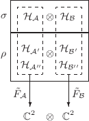
In particular, let
| (7.21) |
where , c.f. Eq. (4.17), is the (unnormalized) maximally entangled state between the spaces and (which have the same dimension), and is the identity matrix acting on (analogously for Bob). After some simple calculations, it can be shown that for any acting on
where stands for the transpose of .1515 15 More generally, for any acting on , any acting on , and any acting on , it can be shown that Hence, the requirement that inequality (7.14) is violated (i.e., ) with , , becomes
| (7.22) |
What remains is to show that there exists some physical state such that the above inequality holds true.
For convenience, in the rest of the proof we allow to be unnormalized. The only constraints on the matrices are then positive semidefiniteness (), and satisfiability of all the inequalities (7.14) in Lemma 15. is now a convex cone, and its dual cone is defined as
| (7.23) |
where are Hermitian matrices. An important point to note now is that Farkas’ Lemma [218] states that all matrices in can be written as non-negative linear combinations of matrices and matrices of the form
| (7.24) |
with and .
We now show that there always exists satisfying inequality (7.22) by supposing otherwise and arriving at a contradiction. Suppose that for all , the converse inequality of Eq. (7.22) holds true, i.e.,
| (7.25) |
It then follows from the definition of , Eq. (7.23), that the matrix belongs to . Applying Farkas’ Lemma [218] we can write
where is a label for matrices of the form given by Eq. (7.24) and is a label for element in . It is easy to see that the above matrix equality is equivalent to the matrix inequality
| (7.26) |
where each is a separable map, c.f. Eq. (7.12), that takes matrices acting on to matrices acting on . The following Lemma, however, requires that this is true only if is separable (see Appendix B.5.1 for details).
Lemma 17.
Let be a family of maps, separable with respect to the partition denoted by the brackets. Let be a unit-trace, PSD matrix acting on such that
| (7.27) |
where is defined in Eq. (7.15), then has to be separable.
Hence, if all are such that none of them can give rise to a Bell-CHSH violation for via the protocol given in Eq. (7.21) (see also Figure 7.2), it must be the case that is a separable state. As a result, the corresponding contrapositive positive statement reads: for every entangled , there exists such that violates the Bell-CHSH inequality via the protocol given by Eq. (7.21). This completes our proof of Theorem 16.
∎
At this stage, it is worth making a few other remarks concerning the nonstandard Bell experiments that we have just described. To fix ideas, we will restrict ourselves to the nontrivial case that both and are members of and where is entangled. Then for to violate the Bell-CHSH inequality via our protocol, it must also be that (1) is entangled and (2) at least one of and has negative partial transposition. That is entangled can be easily seen by following the argument given in the proof of Theorem 16, but with the role of and reversed (pp. 16). On the other hand, it is also not difficult to see that if both and were to have positive partial transposition, then after the local filtering operation given by Eq. (7.21), the resulting two-qubit state would still be PPT [163] and hence separable [162]. Since no separable state can violate the Bell-CHSH inequality, at least one of and must have negative partial transposition.
Meanwhile, we have only required that the ancilla state does not violate the Bell-CHSH inequality, and therefore it may violate other Bell inequalities, like anyone among the zoo of inequalities presented in Sec. 3.3.1 and Sec. 3.3.2. However, even if does violate another Bell inequality, we know by definition that , and thus (with being any separable state) does not violate the Bell-CHSH inequality. Hence, in the Bell-CHSH experiment that we are considering, cannot be replaced by any classical correlations or separable state .
7.5 Conclusion
In this chapter, we have reviewed the phenomenon of hidden nonlocality associated with entangled states, and the various kinds of nonstandard Bell experiments that have been proposed to derive nonclassical correlations from them. To date, it is still not known if all entangled states can violate some Bell inequalities via a nonstandard Bell experiment that only involves the state in question. Given this state of affair, we have looked into the possibility of deriving nonclassical correlations from all bipartite entangled states by considering nonstandard Bell experiments that also involve shared auxiliary states. Evidently, the choice of such an ancilla state cannot be arbitrary. In particular, the protocol that we have considered involves an ancilla state which by itself does not violate the Bell-CHSH inequality even after arbitrary local filtering operations. In the notation that we have developed, we say that . Then, by considering a specific local filtering protocol, we have shown that for every entangled state , there exists an ancilla state such that the combined state does violate the Bell-CHSH inequality after the prescribed local filtering operations.
This provides us with a new way to interpret (bipartite) entanglement in terms of the behavior of the states, in contrast with the usual definition in terms of the preparation of the states. Entangled states are, by definition, the ones that cannot be generated from classical correlations using LOCC. We have shown that in the bipartite case, one can equivalently define entangled states as the ones that cannot be simulated by classical correlations alone.1616 16 However, some nonclassical correlations can be simulated by classical correlations when supplemented with only one bit of classical communication (see, for example Ref. [219] and references therein). In addition, this also gives a conclusive answer to the long-standing question of whether all (bipartite) entangled states can display some hidden nonlocality [53, 38, 39, 31].
Despite that, it is worth reminding that our proof of the key result is a non-constructive one. Therefore, even though we know that there exists some ancilla state such that can lead to observable nonlocality for any entangled , we do not know much about the property of the ancilla state. A natural task that follows from our findings is thus to obtain an explicit expression for the ancilla state for some given . From an experimental point of view, a better understanding of this ancilla state is also relevant, since distillation protocol involving many copies of the same quantum system is hard to implement. Therefore, a protocol to demonstrate nonclassical correlations involving only a single copy of and may be preferable over those other which involve, say, 10 copies of or .
On the other hand, as with the bipartite scenario, there are also mixed multipartite entangled states that admit explicit LHVM for projective measurement [32] (see Sec. 4.3.2.3). An interesting question that follows from the present work is therefore to determine if the current proof of observable nonlocality also generalizes to this more complicated scenario, and hence establishes some kind of equivalence between entanglement and states that cannot always be simulated by classical correlations.
Chapter 8 Conclusion
It is one of the most phenomenal discoveries that quantum mechanical predictions on entangled, spatially separated systems cannot always be given a locally causal description. By now, it is well-known that entanglement is necessary, but may not always be sufficient to demonstrate this fact through a Bell inequality violation in a standard Bell experiment. A nonstandard Bell experiment, which involves local preprocessing and some kind of postselection, may however unveil the nonclassical correlations hidden in some entangled quantum states. Given this state of affairs, this thesis aims to clarify further the relationships between the notions of correlations, Bell inequality violation and quantum entanglement in discrete variable quantum systems. In this chapter, we will summarize our key findings and outline some possible avenues for future research.
Our study began in Chapter 5, where we looked into the problem of determining if a given quantum state can violate some fixed but arbitrary Bell inequality in a standard Bell experiment. This is a high-dimensional variational problem where, in general, nontrivial optimization over the choice of local observables is required. To this end, we have derived two algorithms which can be used to determine, respectively, a lower bound (LB) and an upper bound (UB) on the strength of correlation that a quantum state can offer in a given Bell experiment corresponding to some Bell inequality — a quantity which we have given the notation . Both of these algorithms make use of convex optimization techniques in the form of a semidefinite program (SDP), which is readily solved on a computer. The LB algorithm requires one to solve a series of SDPs iteratively, whereas the UB algorithm provides a hierarchy of SDPs, with each giving a better upper bound on . These algorithms can also be implemented analytically. In fact, we have made use of the UB algorithm to derive a necessary condition for bipartite qudit states with vanishing coherence vectors to violate the Bell-CHSH inequality; a simple implementation of the LB algorithm has also enabled us to rederive the Horodecki criterion for two-qubit states. Since the bounds derived from these algorithm are usually not tight, these algorithms often need to be used in tandem to determine if can violate some Bell inequality .
Next, in Chapter 6, we looked at some of the best known Bell inequalities violations by bipartite quantum states. In particular, using the LB algorithm derived in Chapter 5, we have obtained the local measurements giving the best known Bell-CH, and hence Bell-CHSH inequality violation for arbitrary pure two-qudit states. Then, by establishing a formal equivalence between the -outcome CGLMP inequality and the inequality, we have also obtained the best known violation for the -dimensional isotropic states . Together with the UB algorithm derived in Chapter 5, these best known violations were then used to show that for (arbitrary) bipartite pure two-qudit entangled state , a better Bell-CH inequality violation can be obtained via collective measurements on , i.e., copies of for . The same, however, cannot be said for mixed entangled states. In fact, we have strong numerical evidence suggesting that the maximal Bell-CH inequality violation for some entangled states may not depend on the number of copies . Further numerical evidence even indicates that the set of mixed two-qubit states is dominated by those whose maximal Bell-CH inequality violation remains unchanged even when .
After that, in Chapter 7, we studied the possibility of deriving nonclassical correlations from all entangled states via a nonstandard Bell experiment. In other words, we wanted to know if it is actually possible to demonstrate some kind of observable nonlocality for all entangled states. To this end, we have explicitly characterized the set of bipartite quantum states which do not violate the Bell-CHSH inequality even after arbitrary local filtering operations — a set which we have given the notation . Then, by considering a specific type of local filtering operation, we have (non-constructively) shown that for every bipartite entangled state , there exists an ancilla state such that . Interestingly, this means that even if both and can be simulated, individually, by classical correlations in the most general single-copy nonstandard Bell-CHSH experiment, the combined state cannot be described by classical correlations in some single-copy nonstandard Bell-CHSH experiment. Consequently, we can now define a bipartite entangled state as precisely that which cannot be simulated by classical correlations when one consider all possible experiments that may be performed on in conjunction with non-Bell-CHSH-violating states.
Let us now make some remarks regarding future research. To begin with, we note that possible follow-up projects in relation to the work presented in each chapters have already been presented in some details at the end of the corresponding chapters. As such, we will not try to repeat all of them here, but to merely remind the readers of some of the key ones. Firstly, as one may have noticed, our analysis in this thesis has been carried out exclusively for discrete variable quantum systems and to a large extent, only for bipartite quantum systems. There are, of course, many interesting problems that are associated with Bell inequality violation in multipartite and continuous variable quantum systems. For example, it is still not known if all discrete multipartite pure entangled states can violate a Bell inequality in a standard Bell experiment. In continuous variable quantum systems, it is not even known if all bipartite pure entangled states can violate a Bell inequality. As a result, preliminary investigations on the adaptability of the tools that we have developed here to this latter scenario could be of some use.
Results that we have obtained in Chapter 5, as well as those presented in Ref. [17] have indicated that upper bound techniques similar to those that we have developed in this thesis do allow us to investigate the extent to which quantum mechanics can violate a fixed but arbitrary Bell inequality. Further work on this is clearly desirable as it will help us to learn something about the extreme points of the set of quantum correlations. This is work in progress [197].
Given that we have only got a nonconstructive proof for the nonclassical correlations hidden in an arbitrary entangled state , it would be great if an explicit construction of the ancilla state used in our protocol can be obtained. A general construction of the ancilla state may be formidable, but it would be helpful to at least solve this for some simple cases like Werner states, or more desirably, some bound entangled states. Finally, the arguably most important problem that is left opened from the present work is whether it is also possible to derive some observable, nonclassical correlations from all multipartite entangled quantum states, be it discrete or continuous. Any progress in this regard would certainly help us to improve our understanding of the quantum world, which is always full of surprises.
References
- [1] Y.-C. Liang and A. C. Doherty. Bounds on quantum correlations in Bell-inequality experiments. Physical Review A 75(4), 042103 (2007).
- [2] Y.-C. Liang and A. C. Doherty. Better Bell-inequality violation by collective measurements. Physical Review A 73(5), 052116 (2006).
- [3] Ll. Masanes, Y.-C. Liang, and A. C. Doherty. All bipartite entangled states display some hidden nonlocality. eprint quant-ph/0703268 (2007).
- [4] Y.-C. Liang, Ll. Masanes, and A. C. Doherty. SLOCC convertibility between two-qubit states. eprint quant-ph/0710.5350 (2007).
- [5] J. S. Bell. On the Einstein-Podolsky-Rosen paradox. Physics 1(3), 195 (1964).
- [6] J. F. Clauser, M. A. Horne, A. Shimony, and R. A. Holt. Proposed experiment to test local hidden-variable theories. Physical Review Letters 23, 880 (1969).
- [7] J. F. Clauser and M. A. Horne. Experimental consequences of objective local theories. Phys. Rev. D10(2), 526 (1974).
- [8] A. Peres. All the Bell inequalities. Foundations of Physics 29(4), 589 (1999).
- [9] W. J. Munro, D. F. V. James, A. G. White, and P. G. Kwiat. Maximizing the entanglement of two mixed qubits. Physical Review A 64(3), 030302 (2001).
- [10] T. C. Wei, K. Nemoto, P. M. Goldbart, P. G. Kwiat, W. J. Munro, and F. Verstraete. Maximal entanglement versus entropy for mixed quantum states. Physical Review A 67(2), 022110 (2003).
- [11] L. Derkacz and L. Jakobczyk. Clauser-Horne-Shimony-Holt violation and the entropy-concurrence plane. Physical Review A 72(4), 042321 (2005).
- [12] E. Santos. Entropy inequalities and Bell inequalities for two-qubit systems. Physical Review A 69(2), 022305 (2004).
- [13] E. Santos. Erratum: “Entropy inequalities and Bell inequalities for two-qubit systems” [Phys. Rev. A 69, 022305, (2004)]. Physical Review A 70(5), 059901 (2004).
- [14] T. Ito, H. Imai, and D. Avis. Bell inequalities stronger than the Clauser-Horne-Shimony-Holt inequality for three-level isotropic states. Physical Review A 74(4), 042109 (2006).
- [15] K. G. H. Vollbrecht and R. F. Werner. Entanglement measures under symmetry. Physical Review A 64(6), 062307 (2001).
- [16] A. Acín, T. Durt, N. Gisin, and J. I. Latorre. Quantum nonlocality in two three-level systems. Physical Review A 65(5), 052325 (2002).
- [17] M. Navascués, S. Pironio, and A. Acín. Bounding the set of quantum correlations. Physical Review Letters 98(1), 010401 (2007).
- [18] E. Schrödinger. Discussion of probability relations between separated systems. Proceedings of the Cambridge Philosophical Society 31, 555 (1935).
- [19] E. Schrödinger. Die gegenwrtige situation in der quantenmechanik. Naturwissenschaften 23, 807 (1935).
- [20] A. Einstein, B. Podolsky, and N. Rosen. Can quantum-mechanical description of physical reality be considered complete? Physical Review 47, 777 (1935).
- [21] J. D. Trimmer. The present situation in quantum mechanics: A translation of Schrödinger’s ”cat paradox” paper. Proceedings of the American Physical Society 124(5), 323 (1980).
- [22] A. Einstein. Albert Einstein: Philosopher-Scientist, chap. Reply to Criticisms (Cambridge University Press, 1949).
- [23] J. S. Bell. Einstein-Podolsky-Rosen experiments. In Proceedings of the Symposium on Frontier Problems in High Energy Physics, pp. 33–45 (1976).
- [24] J. S. Bell. On the problem of hidden variables in quantum mechanics. Review of Modern Physics 38, 447 (1966).
- [25] D. Bohm. Quantum Theory (Englewood Cliffs, N.J. : Prentice-Hall, 1951).
- [26] A. Aspect. Bell’s inequality test: more ideal than ever. Nature 398, 189 (1999).
- [27] M. A. Rowe, D. Kielpinski, V. Meyer, C. A. Sackett, W. A. Itano, C. Monroe, and D. J. Wineland. Experimental violation of a Bell’s inequality with efficient detection. Nature 409(6822), 791 (2001).
- [28] P. G. Kwiat, S. Barraza-Lopez, A. Stefanov, and N. Gisin. Experimental entanglement distillation and ’hidden’ non-locality. Nature 409(6823), 1014 (2001).
- [29] R. F. Werner. Quantum states with Einstein-Podolsky-Rosen correlations admitting a hidden-variable model. Physical Review A 40, 4277 (1989).
- [30] R. Horodecki, P. Horodecki, and M. Horodecki. Violating Bell inequality by mixed spin- states: Necessary and sufficient condition. Physics Letters A 200(5), 340 (1995).
- [31] J. Barrett. Nonsequential positive-operator-valued measurements on entangled mixed states do not always violate a Bell inequality. Physical Review A 65(4), 042302 (2002).
- [32] G. Tóth and A. Acín. Genuine tripartite entangled states with a local hidden-variable model. Physical Review A 74(3), 030306 (2006).
- [33] M. L. Almeida, S. Pironio, J. Barrett, G. Tóth, and A. Acín. Noise robustness of the nonlocality of entangled quantum states. Physical Review Letters 99(4), 040403 (2007).
- [34] V. Capasso, D. Fortunato, and F. Selleri. Sensitive observables of quantum mechanics. International Journal of Theoretical Physics 7(5), 319 (1973).
- [35] N. Gisin. Bell inequality holds for all non-product states. Physics Letters A 154(5-6), 201 (1991).
- [36] N. Gisin and A. Peres. Maximal violation of Bell inequality for arbitrarily large spin. Physics Letters A 162(1), 15 (1992).
- [37] J.-L. Chen, C. Wu, L. C. Kwek, and C. H. Oh. Gisin’s theorem for three qubits. Physical Review Letters 93(14), 140407 (2004).
- [38] S. Popescu. Bell’s inequalities and density matrices: Revealing ”hidden” nonlocality. Physical Review Letters 74(14), 2619 (1995).
- [39] N. Gisin. Hidden quantum nonlocality revealed by local filters. Physics Letters A 210(3), 151 (1996).
- [40] A. Peres. Collective tests for quantum nonlocality. Physical Review A 54(4), 2685 (1996).
- [41] A. K. Ekert. Quantum cryptography based on Bell’s theorem. Physical Review Letters 67(6), 661 (1991).
- [42] V. Scarani and N. Gisin. Quantum communication between n partners and Bell’s inequalities. Physical Review Letters 87(11), 117901 (2001).
- [43] A. Acín, N. Gisin, Ll. Masanes, and V. Scarani. Bell’s inequalities detect efficient entanglement. International Journal of Quantum Information 2(1), 23 (2004).
- [44] J. Barrett, L. Hardy, and A. Kent. No signaling and quantum key distribution. Physical Review Letters 95(1), 010503 (2005).
- [45] A. Acín, N. Gisin, and Ll. Masanes. From Bell’s theorem to secure quantum key distribution. Physical Review Letters 97(12), 120405 (2006).
- [46] Ll. Masanes and A. Winter. Unconditional security of key distribution from causality constraints. eprint quant-ph/0606049 (2006).
- [47] H. Buhrman, R. Cleve, and W. van Dam. Quantum entanglement and communication complexity. SIAM Journal On Computing 30(6), 1829 (2000).
- [48] Č. Brukner, M. Żukowski, and A. Zeilinger. Quantum communication complexity protocol with two entangled qutrits. Physical Review Letters 89(19), 197901 (2002).
- [49] Č. Brukner, M. Żukowski, J.-W. Pan, and A. Zeilinger. Bell’s inequalities and quantum communication complexity. Physical Review Letters 92(12), 127901 (2004).
- [50] C. H. Bennett, G. Brassard, C. Crépeau, R. Jozsa, A. Peres, and W. K. Wootters. Teleporting an unknown quantum state via dual classical and Einstein-Podolsky-Rosen channels. Physical Review Letters 70(13), 1895 (1993).
- [51] R. Horodecki, M. Horodecki, and P. Horodecki. Teleportation, Bell’s inequalities and inseparability. Physics Letters A 222, 21 (1996).
- [52] S. Popescu. Bell’s inequalities versus teleportation: What is nonlocality? Physical Review Letters 72(6), 797 (1994).
- [53] N. Gisin. Bell inequalities: many questions, a few answers. eprint quant-ph/0702021 (2007).
- [54] S. Filipp and K. Svozil. Generalizing Tsirelson’s bound on Bell inequalities using a min-max principle. Physical Review Letters 93, 130407 (2004).
- [55] H. Buhrman and S. Massar. Causality and Tsirelson’s bounds. Physical Review A 72(5), 052103 (2005).
- [56] S. Wehner. Tsirelson bounds for generalized Clauser-Horne-Shimony-Holt inequalities. Physical Review A 73(2), 022110 (2006).
- [57] B. F. Toner. Monogamy of nonlocal quantum correlations. eprint quant-ph/0601172 (2006).
- [58] D. Avis, H. Imai, and T. Ito. On the relationship between convex bodies related to correlation experiments with dichotomic observables. Journal of Physics A-Mathematical and General 39(36), 11283 (2006).
- [59] Ll. Masanes. Tight Bell inequality for d-outcome measurements correlations. Quantum Information & Computation 3(4), 345 (2003).
- [60] D. Collins and N. Gisin. A relevant two qubit Bell inequality inequivalent to the CHSH inequality. Journal of Physics A-Mathematical and General 37(5), 1775 (2004).
- [61] D. Avis, H. Imai, T. Ito, and Y. Sasaki. Two-party Bell inequalities derived from combinatorics via triangular elimination. Journal of Physics A-Mathematical and General 38, 10971 (2005).
- [62] I. Pitowsky. Quantum Probability – Quantum Logic, vol. 321 of Lecture Notes in Physics (Springer, Berlin, 1989).
- [63] S. Boyd and L. Vandenberghe. Convex Optimization (New York : Cambridge, 2004).
- [64] L. Vandenberghe and S. Boyd. Semidefinite programming. SIAM Review 38, 49 (1996).
- [65] A. Peres. Quantum Theory : Concepts and Methods (Springer, New York, 1995).
- [66] C. J. Isham. Lectures on Quantum Theory: Mathematical and Structural Foundations (Imperial College Press, London, 1995).
- [67] N. Bohr. Quantum postulate and recent developments in atomism. Naturwissenschaften 16, 245 (1928).
- [68] N. Bohr. The quantum postulate and the recent development of atomic theory. Nature 121, 580 (1928).
- [69] M. O. Scully, B.-G. Englert, and H. Walther. Quantum optical tests of complementarity. Nature 351(6322), 111 (1991).
- [70] L. de Broglie. La mécanique ondulatoire et la structure atomique de la matière et du rayonnement. Journal de Physique et du Radium 8, 225 (1927).
- [71] L. de Broglie. Rapports et Discussions du Cinquième Conseil de Physique Solvay, chap. La nouvelle dynamique des quanta, pp. 105–141 (Paris: Gauthier-Villars, 1928).
- [72] J. von Neumann. Mathematische Grundlagen der Quantenmechanik (Berlin: Springer Verlag, 1932).
- [73] D. Bohm. A suggested interpretation of the quantum theory in terms of ”hidden variables” I. Physical Review 85, 166 (1952).
- [74] D. Bohm. A suggested interpretation of the quantum theory in terms of ”hidden variables” II. Physical Review 85, 180 (1952).
- [75] J. S. Bell. Speakable and Unspeakable in Quantum Mechanics (Cambridge: Cambridge University Press, 1987).
- [76] J. S. Bell. Foundation of Quantum Mechanics. Proceedings of the International School of Physics ‘Enrico Fermi’, course IL, chap. Introduction to the Hidden-Variable Question, pp. 171–181 (Academic, New York, 1971).
- [77] J. S. Bell. Between Science and Technology, chap. La Nouvelle Cuisine, pp. 97–115 (Elsevier/North-Holland, 1990).
- [78] T. Norsen. Against ’realism’. Foundations of Physics 37(3), 311 (2007).
- [79] J. S. Bell. EPR correlations and EPW distributions. Annals of the New York Academy of Sciences 480, 263 (1986).
- [80] B. M. Terhal. Bell inequalities and the separability criterion. Physics Letters A 271(5-6), 319 (2000).
- [81] P. Hyllus, O. Gühne, D. Bruß, and M. Lewenstein. Relations between entanglement witnesses and Bell inequalities. Physical Review A 72(1), 012321 (2005).
- [82] J. F. Clauser and A. Shimony. Bell’s theorem: experimental tests and implications. Reports on Progress in Physics 41, 1881 (1978).
- [83] S. J. Freedman and J. F. Clauser. Experimental test of local hidden-variable theories. Physical Review Letters 28(14), 938 (1972).
- [84] A. Shimony. Bell’s theorem. In E. N. Zalta, ed., The Stanford Encyclopedia of Philosophy (Summer 2005). URL http://plato.stanford.edu/archives/sum2005/entries/bell-theor%em/.
- [85] A. Aspect, J. Dalibard, and G. Roger. Experimental test of Bell’s inequalities using time-varying analyzers. Physical Review Letters 49(25), 1804 (1982).
- [86] T. W. Marshall, E. Santos, and F. Selleri. Local realism has not been refuted by atomic cascade experiments. Physics Letters A 98(1-2), 5 (1983).
- [87] E. Santos. Does quantum mechanics violate the Bell inequalities? Physical Review Letters 66(11), 1388 (1991).
- [88] E. Santos. Critical analysis of the empirical tests of local hidden-variable theories. Physical Review A 46(7), 3646 (1992).
- [89] E. Santos. The failure to perform a loophole-free test of Bell’s inequality supports local realism. Foundations of Physics 34(11), 1643 (2004).
- [90] E. Santos. Bell’s theorem and the experiments: Increasing empirical support for local realism? Studies In History and Philosophy of Modern Physics 36B(3), 544 (2005).
- [91] G. Weihs, T. Jennewein, C. Simon, H. Weinfurter, and A. Zeilinger. Violation of Bell’s inequality under strict Einstein locality conditions. Physical Review Letters 81(23), 5039 (1998).
- [92] E. S. Fry and T. Walther. Quantum [Un]speakables, chap. Atom Based Tests of the Bell Inequalities - the Legacy of John Bell Continues …, pp. 103–117 (Springer: Berlin-Heidelberg-New York, 2002).
- [93] J. Barrett, D. Collins, L. Hardy, A. Kent, and S. Popescu. Quantum nonlocality, Bell inequalities, and the memory loophole. Physical Review A 66(4), 042111 (2002).
- [94] A. Kent. Causal quantum theory and the collapse locality loophole. Physical Review A 72(1), 012107 (2005).
- [95] M. Genovese. Research on hidden variable theories: A review of recent progresses. Physics Reports-Review Section of Physics Letters 413(6), 319 (2005).
- [96] M. Froissart. Constructive generalization of Bell’s inequalities. Nuovo Cimento Della Società Italiana Di Fisica B-General Physics, Relativity, Astronomy and Mathematical Physics and Methods 64(2), 241 (1981).
- [97] A. Garg and N. D. Mermin. Farkas lemma and the nature of reality: Statistical implications of quantum correlations. Foundations of Physics 14(1), 1 (1984).
- [98] I. Pitowsky. Correlation polytopes: their geometry and complexity. Mathematical Programming 50(3), 395 (1991).
- [99] A. Fine. Hidden variables, joint probability, and the Bell inequalities. Physical Review Letters 48(5), 291 (1982).
- [100] A. Garg and N. D. Mermin. Comment on ”hidden variables, joint probability, and the Bell inequalities”. Physical Review Letters 49(3), 242 (1982).
- [101] A. Fine. Fine responds. Physical Review Letters 49(3), 243 (1982).
- [102] A. Garg and N. D. Mermin. Local realism and measured correlations in the spin-s Einstein-Podolsky-Rosen experiment. Physical Review D 27(2), 339 (1983).
- [103] S. Popescu and D. Rohrlich. Quantum nonlocality as an axiom. Foundations of Physics 24(3), 379 (1994).
- [104] R. F. Werner and M. M. Wolf. Bell inequalities and entanglement. Quantum Information and Computation 1, 1 (2001).
- [105] V. Scarani and N. Gisin. Superluminal influences, hidden variables, and signaling. Physics Letters A 295(4), 167 (2002).
- [106] B. Grünbaum. Convex Polytope (Springer, New York, 2003), 2 ed.
- [107] G. M. Ziegler. Lectures on Polytopes (Springer, New York, 1995), 1 ed.
- [108] B. M. Terhal, A. C. Doherty, and D. Schwab. Symmetric extensions of quantum states and local hidden variable theories. Physical Review Letters 90(15), 157903 (2003).
- [109] I. Pitowsky and K. Svozil. Optimal tests of quantum nonlocality. Physical Review A 64(1), 014102 (2001).
- [110] N. D. Mermin. Quantum mechanics vs local realism near the classical limit: A Bell inequality of spin s. Physical Review D 22(2), 356 (1980).
- [111] A. Garg and N. D. Mermin. Bell inequalities with a range of violation that does not diminish as the spin becomes arbitrarily large. Physical Review Letters 49(13), 901 (1982).
- [112] A. Garg and N. D. Mermin. Correlation inequalities and hidden variables. Physical Review Letters 49(17), 1220 (1982).
- [113] N. D. Mermin and G. M. Schwarz. Joint distributions and local realism in the higher-spin Einstein-Podolsky-Rosen experiment. Foundations of Physics 12(2), 101 (1982).
- [114] N. D. Mermin. Generalizations of Bell’s Theorem to higher spins and higher correlations, chap. Fundamental Questions in Quantum Mechanics, pp. 7–20 (Gordon and Breach, 1986).
- [115] R. F. Werner and M. M. Wolf. All-multipartite Bell-correlation inequalities for two dichotomic observables per site. Physical Review A 64(3), 032112 (2001).
- [116] C. Śliwa. Symmetries of the Bell correlation inequalities. Physics Letters A 317(3-4), 165 (2003).
- [117] S. Pironio. Lifting Bell inequalities. Journal of Mathematical Physics 46(6), 062112 (2005).
- [118] N. Brunner and N. Gisin. Partial list of bipartite Bell inequalities with four binary settings. eprint arXiv:0711.3362 (2007).
- [119] D. Avis and T. Ito. New classes of facets of the cut polytope and tightness of Bell inequalities. Discrete Applied Mathematics 155(13), 1689 (2007).
- [120] http://www-imai.is.s.u-tokyo.ac.jp/ tsuyoshi/bell/bell5.html.
- [121] D. Collins, N. Gisin, N. Linden, S. Massar, and S. Popescu. Bell inequalities for arbitrarily high-dimensional systems. Physical Review Letters 88(4), 040404 (2002).
- [122] D. Kaszlikowski, L. C. Kwek, J.-L. Chen, M. Żukowski, and C. H. Oh. Clauser-Horne inequality for three-state systems. Physical Review A 65(3), 032118 (2002).
- [123] N. D. Mermin. Extreme quantum entanglement in a superposition of macroscopically distinct states. Physical Review Letters 65(15), 1838 (1990).
- [124] D. M. Greenberger, M. A. Horne, and A. Zeilinger. Bell’s Theorem, Quantum Theory and Conceptions of the Universe, pp. 69–72 (Kluwer Academics, Dordrecht, 1989).
- [125] D. M. Greenberger, M. A. Horne, and A. Zeilinger. Going beyond Bell’s theorem. eprint arXiv:0712.0921 (2007).
- [126] S. M. Roy and V. Singh. Tests of signal locality and Einstein-Bell locality for multiparticle systems. Physical Review Letters 67(20), 2761 (1991).
- [127] M. Ardehali. Bell inequalities with a magnitude of violation that grows exponentially with the number of particles. Physical Review A 46(9), 5375 (1992).
- [128] A. V. Belinskiǐ and D. N. Klyshko. The interference of light and the Bell theorem. Uspekhi Fizicheskikh Nauk 163(8), 1 (1993).
- [129] A. V. Belinskiǐ and D. N. Klyshko. Interference of light and Bell’s theorem. Physics-Uspekhi 36(8), 653 (1993).
- [130] N. Gisin and H. Bechmann-Pasquinucci. Bell inequality, Bell states and maximally entangled states for n qubits. Physics Letters A 246(1-2), 1 (1998).
- [131] M. Żukowski and Č. Brukner. Bell’s theorem for general n-qubit states. Physical Review Letters 88(21), 210401 (2002).
- [132] H. Weinfurter and M. Żukowski. Four-photon entanglement from down-conversion. Physical Review A 6401(1), 010102 (2001).
- [133] X. H. Wu and H. S. Zong. Violation of local realism by a system with n spin-1/2 particles. Physical Review A 68(3), 032102 (2003).
- [134] W. Laskowski, T. Paterek, M. Żukowski, and Č. Brukner. Tight multipartite Bell’s inequalities involving many measurement settings. Physical Review Letters 93(20), 200401 (2004).
- [135] M. Żukowski. On tight multiparty Bell inequalities for many settings. Quantum Information Processing 5(4), 287 (2006).
- [136] M. Żukowski. All tight multipartite Bell corelation inequalities for three dichotomic observables per observer. eprint quant-ph/0611086 (2006).
- [137] M. Wieśniak, P. Badzia̧g, and M. Żukowski. Explicit form of correlation-function three-setting tight Bell inequalities for three qubits. Physical Review A 76(1), 012110 (2007).
- [138] A. Acín, J.-L. Chen, N. Gisin, D. Kaszlikowski, L. C. Kwek, C. H. Oh, and M. Żukowski. Coincidence Bell inequality for three three-dimensional systems. Physical Review Letters 92(25), 250404 (2004).
- [139] V. Scarani, A. Acín, E. Schenck, and M. Aspelmeyer. Nonlocality of cluster states of qubits. Physical Review A 71(4), 042325 (2005).
- [140] K. Chen, S. Albeverio, and S. M. Fei. Two-setting Bell inequalities for many qubits. Physical Review A 74(5), 050101 (2006).
- [141] C. Wu, Y. Yeo, L. C. Kwek, and C. H. Oh. Quantum nonlocality of four-qubit entangled states. Physical Review A 75(3), 032332 (2007).
- [142] L. A. Khalfin and B. S. Tsirelson. Quantum classical correspondence in the light of Bells inequalities. Foundations of Physics 22(7), 879 (1992).
- [143] B. S. Cirelson. Quantum generalizations of Bell’s inequality. Lett. Math. Phys. 4, 93 (1980).
- [144] B. S. Tsirelson. Quantum analogues of Bell’s inequalities. The case of two spatially divided domains. Zapiski Nauchnykh Seminarov Leningradskogo Otdeleniya Matematicheskogo Instituta im. V. A. Steklova AN SSSR 142, 174 (1985).
- [145] B. S. Tsirel’son. Quantum analogues of the Bell inequalities. The case of two spatially separated domains. Journal of Soviet Mathematics 36(4), 557 (1987).
- [146] I. Pitowsky. The range of quantum probability. Journal of Mathematical Physics 27(6), 1556 (1986).
- [147] M. Żukowski, R. Horodecki, M. Horodecki, and P. Horodecki. Generalized quantum measurements and local realism. Physical Review A 58(3), 1694 (1998).
- [148] A. Cabello. How much larger quantum correlations are than classical ones. Physical Review A 72(1), 012113 (2005).
- [149] M. Żukowski. Some news about Bell inequalities. Journal of Modern Optics 50(6-7), 1151 (2003).
- [150] D. Jonathan and M. B. Plenio. Minimal conditions for local pure-state entanglement manipulation. Physical Review Letters 83(7), 1455 (1999).
- [151] J. Degorre, S. Laplante, and J. Roland. Simulating quantum correlations as a distributed sampling problem. Physical Review A 72(6), 062314 (2005).
- [152] M. A. Nielsen and I. L. Chuang. Quantum Computation and Quantum Information (Cambridge ; New York : Cambridge University Press, 2000).
- [153] A. Acín, N. Gisin, and B. Toner. Grothendieck’s constant and local models for noisy entangled quantum states. Physical Review A 73(6), 062105 (2006).
- [154] J. L. Krivine. Grothendieck constants and positive type functions on spheres. Advances In Mathematics 31(1), 16 (1979).
- [155] M. Horodecki and P. Horodecki. Reduction criterion of separability and limits for a class of distillation protocols. Physical Review A 59(6), 4206 (1999).
- [156] V. M. Kendon, K. Zyczkowski, and W. J. Munro. Bounds on entanglement in qudit subsystems. Physical Review A 66(6), 062310 (2002).
- [157] M. A. Nielsen. Conditions for a class of entanglement transformations. Physical Review Letters 83(2), 436 (1999).
- [158] T. Eggeling and R. F. Werner. Separability properties of tripartite states with symmetry. Physical Review A 63(4), 042111 (2001).
- [159] A. Acín, D. Bruß, M. Lewenstein, and A. Sanpera. Classification of mixed three-qubit states. Physical Review Letters 87(4), 040401 (2001).
- [160] P. Horodecki. Separability criterion and inseparable mixed states with positive partial transposition. Physics Letters A 232(5), 333 (1997).
- [161] A. Peres. Separability criterion for density matrices. Physical Review Letters 77(8), 1413 (1996).
- [162] M. Horodecki, P. Horodecki, and R. Horodecki. Separability of mixed states: Necessary and sufficient conditions. Physics Letters A 223(1-2), 1 (1996).
- [163] M. Horodecki, P. Horodecki, and R. Horodecki. Mixed state entanglement and distillation: Is there a ”bound” entanglement in nature? Physical Review Letters 80(24), 5239 (1998).
- [164] C. H. Bennett, G. Brassard, S. Popescu, B. Schumacher, J. A. Smolin, and W. K. Wootters. Purification of noisy entanglement and faithful teleportation via noisy channels. Physical Review Letters 76(5), 722 (1996).
- [165] R. F. Werner and M. M. Wolf. Bell’s inequalities for states with positive partial transpose. Physical Review A 61(6), 062102 (2000).
- [166] W. Dür. Multipartite bound entangled states that violate Bell’s inequality. Physical Review Letters 87(23), 230402 (2001).
- [167] D. M. Greenberger, M. Horne, A. Shimony, and A. Zeilinger. Bell theorem without inequalities. American Journal of Physics 58(12), 1131 (1990).
- [168] A. Acín. Distillability, Bell inequalities, and multiparticle bound entanglement. Physical Review Letters 88(2), 027901 (2002).
- [169] A. Acín, V. Scarani, and M. M. Wolf. Bell’s inequalities and distillability in n-quantum-bit systems. Physical Review A 66(4), 042323 (2002).
- [170] C. H. Bennett, D. P. DiVincenzo, T. Mor, P. W. Shor, J. A. Smolin, and B. M. Terhal. Unextendible product bases and bound entanglement. Physical Review Letters 82(26), 5385 (1999).
- [171] A. C. Doherty, P. A. Parrilo, and F. M. Spedalieri. Distinguishing separable and entangled states. Physical Review Letters 88(18), 187904 (2002).
- [172] A. C. Doherty, P. A. Parrilo, and F. M. Spedalieri. Complete family of separability criteria. Physical Review A 69(2), 022308 (2004).
- [173] B. M. Terhal, A. C. Doherty, and D. Schwab. Local hidden variable theories for quantum states. eprint quant-ph/0210053 (2002).
- [174] P. Horodecki, M. Horodecki, and R. Horodecki. Bound entanglement can be activated. Physical Review Letters 82(5), 1056 (1999).
- [175] V. Scarani and N. Gisin. Spectral decomposition of Bell’s operators for qubits. Journal of Physics A-Mathematical and General 34(30), 6043 (2001).
- [176] M. Żukowski, Č. Brukner, W. Laskowski, and M. Wiesniak. Do all pure entangled states violate Bell’s inequalities for correlation functions? Physical Review Letters 88(21), 210402 (2002).
- [177] C. Wu, J.-L. Chen, L. C. Kwek, and C. H. Oh. Quantum nonlocality of n-qubit W states. Physical Review A 73(1), 012310 (2006).
- [178] S. L. Braunstein, A. Mann, and M. Revzen. Maximal violation of Bell inequalities for mixed states. Physical Review Letters 68(22), 3259 (1992).
- [179] M. M. Deza and M. Laurent. Geometry of cuts and metrics. In Algorithms and Combinatorics, vol. 15 (Springer, New York, 1997).
- [180] S. Popescu and D. Rohrlich. Which states violate Bell’s inequality maximally? Physics Letters A 169(6), 411 (1992).
- [181] A. Cabello. Proposed experiment to test the bounds of quantum correlations. Physical Review Letters 92(6), 060403 (2004).
- [182] F. A. Bovino, G. Castagnoli, I. P. Degiovanni, and S. Castelletto. Experimental evidence for bounds on quantum correlations. Physical Review Letters 92(6), 060404 (2004).
- [183] P. A. Parrilo. Semidefinite programming relaxations for semialgebraic problems. Mathematical Programming 96(2), 293 (2003).
- [184] J. B. Lasserre. Global optimization with polynomials and the problem of moments. Siam J. Optim. 11(3), 796 (2001).
- [185] J. Eisert, P. Hyllus, O. Gühne, and M. Curty. Complete hierarchies of efficient approximations to problems in entanglement theory. Physical Review A 70(6), 062317 (2004).
- [186] R. A. Horn and C. R. Johnson. Matrix Analysis (Cambridge University Press, New York, NY, USA, 1990).
- [187] G. Strang. Linear Algebra and Its Applications (Harcourt Brace, San Diego, 1988), 3rd ed.
- [188] C. W. Helstrom. Quantum Detection and Estimation Theory (Academic Press, New York, 1976).
- [189] R. Cleve, P. Høyer, B. Toner, and J. Watrous. Consequences and limits of nonlocal strategies. In Proceedings of the 19th IEEE Annual Conference on Computational Complexity, pp. 236–249 (2004).
- [190] S. Prajna, A. Papachristodoulou, P. Seiler, and P. A. Parrilo. SOSTOOLS: Sum of squares optimization toolbox for MATLAB (2004).
- [191] S. Prajna, A. Papachristodoulou, P. Seiler, and P. A. Parrilo. SOSTOOLS and its control applications. Lecture Notes in Control and Information Sciences 312, 273 (2005).
- [192] K. Schmüdgen. The k-moment problem for compact semi-algebraic sets. Mathematische Annalen 289(2), 203 (1991).
- [193] M. S. Byrd and N. Khaneja. Characterization of the positivity of the density matrix in terms of the coherence vector representation. Physical Review A 68(6), 062322 (2003).
- [194] G. Kimura. The Bloch vector for n-level systems. Physics Letters A 314(5-6), 339 (2003).
- [195] F. Verstraete and M. M. Wolf. Entanglement versus Bell violations and their behavior under local filtering operations. Physical Review Letters 89(17), 170401 (2002).
- [196] J. W. Nie, J. Demmel, and B. Sturmfels. Minimizing polynomials via sum of squares over the gradient ideal. Mathematical Programming 106(3), 587 (2006).
- [197] A. C. Doherty, Y.-C. Liang, B. Toner, and S. Wehner. The quantum moment problem and bounds on entangled multi-prover games. (in preparation) (2007).
- [198] A. Peres. Finite violation of a Bell inequality for arbitrarily large spin. Physical Review A 46, 4413 (1992).
- [199] D. Kaszlikowski, P. Gnaciński, M. Żukowski, W. Miklaszewski, and A. Zeilinger. Violations of local realism by two entangled n-dimensional systems are stronger than for two qubits. Physical Review Letters 85(21), 4418 (2000).
- [200] L.-B. Fu, J.-L. Chen, and X.-G. Zhao. Maximal violation of the Clauser-Horne-Shimony-Holt inequality for two qutrits. Physical Review A 68(2), 022323 (2003).
- [201] L.-B. Fu, J.-L. Chen, and S.-G. Chen. Maximal violation of Clauser-Horne-Shimony-Holt inequality for four-level systems. Physical Review A 69(3), 034305 (2004).
- [202] S. Popescu and D. Rohrlich. Generic quantum nonlocality. Physics Letters A 166(5-6), 293 (1992).
- [203] E. Schmidt. Zur theorie der linearen und nichtlinearen integralgleighungen. Math. Annalen. 63, 433 (1906).
- [204] S. M. Barnett and S. J. D. Phoenix. Bell inequality and the Schmidt decomposition. Physics Letters A 167(3), 233 (1992).
- [205] J.-L. Chen, D. Kaszlikowski, L. C. Kwek, C. H. Oh, and M. Żukowski. Entangled three-state systems violate local realism more strongly than qubits: An analytical proof. Physical Review A 64(5), 052109 (2001).
- [206] C. H. Bennett, H. J. Bernstein, S. Popescu, and B. Schumacher. Concentrating partial entanglement by local operations. Physical Review A 53(4), 2046 (1996).
- [207] K. Zyczkowski, P. Horodecki, A. Sanpera, and M. Lewenstein. Volume of the set of separable states. Physical Review A 58(2), 883 (1998).
- [208] O. Krüger and R. Werner. Some open problems in quantum information theory. eprint quant-ph/0504166 (2005).
- [209] Ll. Masanes. Asymptotic violation of Bell inequalities and distillability. Physical Review Letters 97(5), 050503 (2006).
- [210] Ll. Masanes. All bipartite entangled states are useful for information processing. Physical Review Letters 96(15), 150501 (2006).
- [211] K. Kraus. General state changes in quantum theory. Annals of Physics 64(2), 311 (1971).
- [212] K. Kraus. States, effects, and operations : fundamental notions of quantum theory : lectures in mathematical physics at the University of Texas at Austin (Springer, Berlin, 1983).
- [213] W. Dür, G. Vidal, and J. I. Cirac. Three qubits can be entangled in two inequivalent ways. Physical Review A 62(6), 062314 (2000).
- [214] M. Horodecki, P. Horodecki, and R. Horodecki. Inseparable two spin-1/2 density matrices can be distilled to a singlet form. Physical Review Letters 78(4), 574 (1997).
- [215] B. G. Englert and N. Metwally. Separability of entangled q-bit pairs. Journal of Modern Optics 47(12), 2221 (2000).
- [216] R. Bhatia. Matrix Analysis (Springer, New York, 1996).
- [217] R. Horodecki and M. Horodecki. Information-theoretic aspects of inseparability of mixed states. Physical Review A 54(3), 1838 (1996).
- [218] B. D. Craven and J. J. Koliha. Generalizations of Farkas theorem. Siam Journal on Mathematical Analysis 8(6), 983 (1977).
- [219] B. F. Toner and D. Bacon. Communication cost of simulating Bell correlations. Physical Review Letters 91(18), 187904 (2003).
- [220] http://www.physics.uq.edu.au/qisci/yerng/.
- [221] A. Jamiołkowski. Linear transformations which preserve trace and positive semidefiniteness of operators. Reports on Mathematical Physics 3(4), 275 (1972).
- [222] M.-D. Choi. Completely positive linear maps on complex matrices. Linear Algebra and its Applications 10(3), 285 (1975).
- [223] V. P. Belavkin and P. Staszewski. A Radon-Nikodym theorem for completely positive maps. Reports on Mathematical Physics 24(1), 49 (1986).
- [224] E. M. Rains. Entanglement purification via separable superoperators. e-print quant-ph/9707002 (1997).
- [225] V. Vedral and M. B. Plenio. Entanglement measures and purification procedures. Physical Review A 57(3), 1619 (1998).
- [226] C. H. Bennett, D. P. DiVincenzo, C. A. Fuchs, T. Mor, E. Rains, P. W. Shor, J. A. Smolin, and W. K. Wootters. Quantum nonlocality without entanglement. Physical Review A 59(2), 1070 (1999).
- [227] J. I. Cirac, W. Dur, B. Kraus, and M. Lewenstein. Entangling operations and their implementation using a small amount of entanglement. Physical Review Letters 86(3), 544 (2001).
Appendix A Bell-diagonal Preserving Separable Maps
In this Appendix we classify the four-qubit states that commute with , where and are arbitrary members of the Pauli group. We characterize the set of separable states for this class, in terms of a finite number of entanglement witnesses. Equivalently, we characterize the set of two-qubit, Bell-diagonal-preserving, completely positive maps (henceforth abbreviated as CPM) that are separable. These separable CPMs correspond to protocols that can be implemented with stochastic local quantum operations assisted by classical communication (SLOCC). Explicit characterization of these CPMs is an essential ingredient of the proof of Lemma 17.
A.1 Four-qubit Separable States with Symmetry
In this section, we will characterize the set of separable states commuting with , where and are arbitrary members of the Pauli group. Let us begin by reminding the reader about an important property of two-qubit states which commute with all unitaries of the form , where is an arbitrary member of the Pauli group. The Pauli group is generated by the Pauli matrices , Eq, (2.6), and has 16 elements. The representation comprises four 1-dimensional irreducible representations, each acting on the subspace spanned by one vector of the Bell basis11 1 These states are more conventionally denoted by , , , .
| (A.1a) | ||||
| (A.1b) | ||||
This implies that [15] any two-qubit state which commutes with can be written as , where is the Bell projector. With this information in mind, we are now ready to discuss the case that is of our interest.
We would like to characterize the set of four-qubit states which commute with all unitaries , where and are members of the Pauli group. Let us denote this set of states by and the state space of as , where , etc. are Hilbert spaces of the constituent qubits. In this notation, both the subsystems associated with and that with have symmetry and hence are linear combinations of Bell-diagonal projectors [15].
Our aim in this section is to provide a full characterization of the set of that are separable between and (see Figure A.1). Throughout this section, a state is said to be separable if and only if it is separable between and .

The symmetry of allows one to write it as a non-negative combination of (tensored-) Bell projectors:
| (A.2) |
where the Bell projector before and after the tensor product, respectively, acts on and (Figure A.1). Thus, any state can be represented in a compact manner, via the corresponding matrix . More generally, any operator acting on the Hilbert space and having the symmetry admits a matrix representation via:
| (A.3) |
where is now not necessarily non-negative. When there is no risk of confusion, we will also refer to and , respectively, as a state and an operator having this symmetry.
Evidently, in this representation, an operator is non-negative if and only if all entries in the corresponding matrix are non-negative. Notice also that by appropriate local unitary transformation, one can swap any with any other , while keeping all the other , unaffected. Here, the term local is used with respect to the and partitioning. Specifically, via the local unitary transformation
| (A.4) |
one can swap and while leaving all the other Bell projectors unaffected. In terms of the corresponding matrix representation, the effect of such local unitaries on amounts to permutation of the rows and/or columns of . For brevity, in what follows, we will say that two matrices and are local-unitarily equivalent if we can obtain by simply permuting the rows and/or columns of and vice versa. A direct consequence of this observation is that if represents a separable state, so is any other that is obtained from by independently permuting any of its rows and/or columns.
Before we state the main result of this section, let us introduce one more definition.
Definition 18.
Let be the convex hull of the states
| (A.5) |
and the states that are local-unitarily equivalent to these two.
Simple calculations show that with respect to the and partitioning, , are separable. In particular, when written in the product basis of , it can be shown that admits the following convex decomposition in terms of separable states:
| (A.6) |
Likewise, it can be shown that admits the following convex decomposition in terms of product states:
| (A.7) |
Hence, is a separable subset of . The main result of this section consists of showing the converse, and hence the following theorem.
Theorem 19.
is the set of states in that are separable with respect to the and partitioning.
Now, we note that is a convex polytope. Its boundary is therefore described by a finite number of facets [106]. Hence, to prove the above theorem, it suffices to show that all these facets correspond to valid entanglement witnesses. Denoting the set of facets by . Then, using the software PORTA,22 2 This software package, which stands for POlyhedron Representation Transformation Algorithm, is available at http://www.zib.de/Optimization/Software/Porta/ the nontrivial facets were found to be equivalent under local unitaries to one of the following:
Apart from these, there is also a facet whose only nonzero entry is . and the operators local-unitarily equivalent to it give rise to positive definite matrices [c.f. Eq. (A.24)], and thus correspond to trivial entanglement witnesses. On the other hand, it is also not difficult to verify that (and operators equivalent under local unitaries) are decomposable and therefore demand that remains positive semidefinite after partial transposition. These are all the entanglement witnesses that arise from the positive partial transposition requirement [161, 162] for separable states.
To complete the proof of Theorem 19, it remains to show that , , give rise to Hermitian matrices
| (A.24) |
that are valid entanglement witnesses, i.e., for any separable . It turns out that this can be proved with the help of the following lemma from Ref. [171, 172].
Lemma 20.
For a given Hermitian matrix acting on , with and , if there exists , positive semidefinite acting on and a subset of the tensor factors such that
| (A.25) |
where is the projector onto the symmetric subspace of (likewise for ) and refers to partial transposition with respect to the subsystem , then is a valid entanglement witness across and , i.e., for any state that is separable with respect to the and partitioning.
Proof.
Denote by the subsystem associated with the -th copy of in ; likewise for . To prove the above lemma, let and be (unit) vectors, and for definiteness, let then it follows that
where is the complex conjugate of . We have made use of the identity (likewise for ) in the second and third equality, Eq. (A.25) in the second equality, and the positive semidefiniteness of . To cater for general , we just have to modify the second to last line of the above computation accordingly (i.e., to perform complex conjugation on all the states in the set ) and the proof will proceed as before. ∎
More generally, let us remark that instead of having one on the rhs of Eq. (A.25), one can also have a sum of different ’s, with each of them partial transposed with respect to different subsystems . Clearly, if the given admits such a decomposition, it is also an entanglement witness [171, 172]. For our purposes these more complicated decompositions do not offer any advantage over the simple decomposition given in Eq. (A.25).
By solving some appropriate SDPs (Appendix C.3.3), we have found that when , and , there exist some , such that Eq. (A.25) holds true for each . Due to space limitations, the analytic expression for these ’s will not be reproduced here but are made available online at Ref. [220]. For , the fact that the corresponding is a witness can even be verified by considering , and . In this case, . If we label the local basis vectors by , the corresponding reads
where we have separated ’s degree of freedom from ’s ones by comma.33 3 Note that to verify against Eq. (A.25), one should also rewrite obtained in Eq. (A.24) in the appropriate tensor-product basis such that acts on . This completes the proof for Theorem 19.
An immediate corollary of the above characterization is that we now know exactly the set of Bell-diagonal preserving transformations that can be performed locally on a Bell-diagonal state. In what follows, we will make use of the Choi-Jamiołkowski isomorphism [221, 222, 223], i.e., the one-to-one correspondence between CPM and quantum state, to make these SLOCC transformations explicit.
A.2 Separable Maps and SLOCC
Now, let us recall some well-established facts about CPM. To begin with, a separable CPM, denoted by takes the following form [224, 225]
| (A.26) |
where acts on , acts on , acts on .44 4 Following Kraus’ work on CPM [211, 212], this specific form of the CPM is also known as a Kraus decomposition of the CPM, with each in the sum conventionally called the Kraus operator associated with the CPM.
If, moreover,
| (A.27) |
the map is trace-preserving, i.e., if is normalized, so is the output of the map . Equivalently, the trace-preserving condition demands that the transformation from to can always be achieved with certainty. It is well-known that all LOCC transformations are of the form Eq. (A.26) but the converse is not true [226].
However, if we allow the map to fail with some probability , the transformation from to can always be implemented probabilistically via LOCC. In other words, if we do not impose Eq. (A.27), then Eq. (A.26) represents, up to some normalization constant, the most general LOCC possible on a bipartite quantum system. These are the SLOCC transformations [213].
To see that Eq. (A.26) can always be realized with some non-zero probability of success, we first note that each of the terms in the decomposition can always be implemented with some probability of success. For instance, if they wish to implement the term in Eq. (A.26), i.e., — which by itself represents uncorrelated local quantum operations on the individual subsystems, they can do that by just by applying some local unitary transformation and/or measurement on their local subsystem. With the help of classical communication, they can then postselect on the desired outcomes to achieve the transformation .
With that in mind, it is then easy to see that implementation of the separable map can be carried out by probabilistically selecting the term to implement in the separable map given by Eq. (A.26). Party can first toss a coin to decide on the term in the decomposition [c.f. Eq. (A.26)] that she would like to implement for that run of the experiment and communicate this outcome to Bob. They then both perform appropriate local operations and postselection to achieve the desired transformation with some probability. Clearly, since each term in Eq. (A.26) can be implemented with some non-zero probability of success, so can the separable map given by Eq. (A.26).
Now, to make a connection between the set of SLOCC transformations and the set of states that we have characterized in Sec. A.1, let us also recall the Choi-Jamiołkowski isomorphism [221, 222, 223] between CPM and quantum states: for every (not necessarily separable) CPM there is a unique — again, up to some positive constant — quantum state corresponding to :
| (A.28) |
where is the unnormalized maximally entangled state of dimension (likewise for ). In Eq. (A.28), it is understood that only acts on the “in” space of and . Clearly, the state acts on a Hilbert space of dimension , where is the dimension of .
Conversely, given a state acting on , the corresponding action of the CPM on some acting on reads:
| (A.29) |
where denotes transposition of in some local bases of . For a trace-preserving CPM, it then follows that we must have . A point that should be emphasized now is that is a separable map, Eq. (A.26), if and only if the corresponding given by Eq. (A.28) is separable across and [227]. Moreover, at the risk of repeating ourselves, the map derived from a separable can always be implemented locally, although it may only succeed with some (nonzero) probability. Hence, if we are only interested in transformations that can be performed locally, and not the probability of success in mapping , the normalization constant as well as the normalization of becomes irrelevant. This is the convention that we will adopt for the rest of this Appendix.
A.3 Bell-diagonal Preserving SLOCC Transformations
We shall now apply the isomorphism to the class of states that we have characterized in Sec. A.1. In particular, if we identify , , and with, respectively, , , and , it follows from Eq. (A.2) and Eq. (A.29) that for any two-qubit state , the action of the CPM derived from reads:
| (A.30) |
Hence, under the action of , any is transformed to another two-qubit state that is diagonal in the Bell basis, i.e., a Bell-diagonal state. In particular, for a Bell-diagonal , i.e.,
| (A.31) |
the map outputs another Bell-diagonal state
| (A.32) |
It is worth noting that for a general , is not proportional to the identity matrix, therefore some of the CPMs derived from are intrinsically non-trace-preserving.55 5 The derived from in Eq. (A.5) is an example of this sort. In fact, in this case, if the input state has no support on nor , the map always outputs the zero matrix.
By considering the convex cone66 6 Since the mapping from any to a separable CPM via Eq. (A.29) is only defined up to a positive constant, for the subsequent discussion, we might as well consider the cone generated by . of separable states that we have characterized in Sec. A.1, we therefore obtain the entire set of Bell-diagonal preserving SLOCC transformations. Among them, we note that the extremal maps, i.e., those derived from Eq. (A.5), admit simple physical interpretations and implementations. In particular, the extremal separable map for , and the maps that are related to it by local unitaries, correspond to permutation of the input Bell projectors — which can be implemented by performing appropriate local unitary transformations. The other kind of extremal separable map, derived from , corresponds to making a measurement that determines if the initial state is in a subspace spanned by a given pair of Bell states and if successful discarding the input state and replacing it by an equal but incoherent mixture of two of the Bell states. This operation can be implemented locally since the equally weighted mixture of two Bell states is a separable state and hence both the measurement step and the state preparation step can be implemented locally.
Appendix B Some Miscellaneous Calculations
B.1 Classical Correlations and Bell’s Theorems
B.1.1 Equivalence between the CGLMP and inequality
In this section, we will provide a proof that the CGLMP inequality for outcomes, Eq. (3.36), is equivalent to the inequality, Eq. (3.35). For the purpose of this proof, we will rewrite the CGLMP inequality, Eq. (3.36), by shifting the constant “2” to the lhs of the inequality, namely,
| (B.1) |
where we remind the reader that expression such as in the above inequality is understood to be evaluated modulo . For ease of reference, we will also reproduce the inequality as follow:
| (3.35) |
Moreover, we shall make use of the matrix representation of a Bell inequality for probabilities introduced in Eq. (3.16) – Eq. (3.20).
Let us begin by showing the equivalence explicitly for . In this case, the lhs of inequality (B.1) can be represented by the following matrix of coefficients11 1 Notice that here, we are writing each block matrix in full dimension, i.e., each block is of dimension ., c.f. Eq. (3.19) and Eq. (3.20),
| where we recall that coefficients associated with Alice’s (Bob’s) local measurement setting are separated by a single horizontal (vertical) line; coefficients associated with marginal probabilities are separated from the others via double horizontal (vertical) lines. | ||||
Now, let us make use of the no-signaling condition, Eq. (3.5) to express the joint probabilities associated with Alice’s third measurement outcome in terms of marginal probabilities and the other joint probabilities for . For example, doing this for , amounts to subtracting every entry in the second column of the block matrix by the entry and adding this specific entry to the marginal entry directly above it. Repeating this for all combinations of , and gives rise to an equivalent inequality with matrix of coefficients given by
Next, let us also make use of the no-signaling condition to express the joint probabilities associated with Bob’s third measurement outcome in terms of marginal probabilities and the other joint probabilities for . In particular, for ,, this amounts to subtracting every entry in the second row of the block matrix by the entry and adding this specific entry to the marginal entry that is on the same row. Doing this for all combinations of , and gives rise to another equivalent inequality with matrix of coefficients given by
Then, by using the normalization condition, c.f. Eq. (3.4),
| (B.2y) |
we can further express in terms of for . In terms of the matrix of coefficients, this amounts to subtracting every entry in by and adding this specific entry to . Writing this out explicitly, we get the matrix of coefficients for a fourth equivalent inequality:
What remains to be done now is to swap all of Bob’s first and second measurement outcomes, which gives a fifth equivalent inequality with matrix of coefficients:
which can be seen to be equivalent to the inequality, Eq. (3.32).
In exactly the same manner, we see that for , we have
then, by zeroing the coefficients associated with and via the no-signaling condition, Eq. (3.5), we get
Finally, by zeroing using Eq. (B.2y) and swapping Bob’s measurement outcomes, , we end up with an equivalent inequality with matrix of coefficients:
is thus equivalent to the inequality, c.f. Eq. (3.34).
More generally, we can prove that is equivalent to by generalizing the above procedures. Firstly, we note that the matrix of coefficients for the -outcome CGLMP inequality, Eq. (B.1), is made up from blocks of circulant matrices , with entries given by
| (B.3a) | |||
| (B.3b) | |||
| and marginal blocks , , : | |||
| (B.3c) | |||
where is an null vector.
As in Eq. (B.1.1), we will now make use of the no-signaling condition, Eq. (3.5), to zero the coefficients associated with the joint probabilities . This gives rise to an equivalent inequality whose matrix of coefficients is related to the original one, by
Next, we will again make use of the no-signaling condition, but to instead zero the coefficients associated with the joint probabilities [c.f. Eq. (B.1.1)]. This gives rise to another equivalent inequality whose matrix of coefficients is related to the existing one, by
Now, we will make use of the normalization of marginal probabilities, Eq. (B.2y), to zero the coefficients associated with the marginal probabilities . This gives rise to another equivalent inequality whose matrix of coefficients is related to the existing one, by
More explicitly, it is easy to check that the matrix of coefficients reads
| (B.4k) | |||
Finally, by swapping Bob’s measurement outcomes, for all , and , it is readily seen that the matrix of coefficients for this fifth equivalent inequality is related to that of by
| (B.5) |
and hence the CGLMP inequality with outcomes, Eq. (B.1), is equivalent to the inequality. Clearly, since the two inequalities, Eq. (3.36) and Eq. (B.1), are identical up to simple algebraic manipulations, the inequality must also be equivalent to the CGLMP inequality written in the form of Eq. (3.36). In particular, if we denote by and , respectively, the Bell operator derived from Eq. (3.36) and Eq. (3.35). Then, for any quantum state , the expectation values of these Bell operators with respect to are related by
| (6.8) |
B.2 Quantum Correlations and Locally Causal Quantum States
B.2.1 Convexity of Non-Bell-Inequality-Violating States
Here, we will prove that the set of quantum states not violating a given Bell inequality in the sense of Definition 7 is convex. Let us denote by the Bell operator associated with a Bell inequality and the set of quantum states not violating via a standard Bell experiment. A quantum state if
| (B.6) |
Clearly, this implies that for any local observables constituting the Bell operator , we must have
| (B.7) |
Now, let two quantum states . Then, for any convex combination of them, i.e.,
| (B.8) |
we see that
Since this is true for any local observables constituting , we must have
| (B.9) |
That is, is also a member of , and hence is a convex set. Moreover, since this is true for an arbitrary Bell inequality, it follows that the set of NBIV quantum states, is also convex.
B.3 Bounds on Quantum Correlations in Standard Bell Experiments
B.3.1 Bell-CH Inequality and Full Rank Projector
In this section, we will prove that the Bell-CH inequality with only two possible outcomes cannot be violated if any of the POVM elements involved is a full rank projector.22 2 This necessarily implies that the complementary POVM element is a zero matrix. For that matter, it suffices to show that in any of these scenarios, the resulting Bell operator is strictly negative semidefinite (NSD), since the trace of a positive semidefinite (PSD) matrix against an NSD matrix cannot be positive.
Now, let us recall that for a two-outcome Bell experiment, the Bell-CH operator can be written as
| (5.39) |
Then, by utilizing the normalization of POVM elements, Eq. (4.1a), we see that when
- 1.
, ,
- 2.
, ,
- 3.
, ,
- 4.
, ,
Since the Bell-CH inequality is symmetrical with respect to swapping the two parties, exactly the same argument can be applied to show that the resulting Bell-CH operator is NSD if any of Alice’s POVM element is a full rank projector. Hence, the Bell-CH inequality cannot be violated in a standard Bell experiment involving at most two possible outcomes and where one of the measurement devices always gives the same measurement outcome.
B.3.2 Derivation of Horodecki’s Criterion using LB
In order to determine if a general two-qubit state violates the Bell-CH inequality, Eq. (3.23), we will have to first obtain an explicit expression for . This can be done, for example, by evaluating Eq. (5.15) which, in turn, requires us to know the eigenvalues of , Eq. (5.13) for all .
In this regard, let us note that for the Bell-CH inequality, we always have
| (B.10a) | |||
| (B.10b) | |||
| (B.10c) | |||
When Alice’s choice of POVM is given by Eq. (5.40), it follows from Eq. (5.37) that the above expressions can be written more explicitly as
which gives, respectively, eigenvalues
| (B.11) |
where and are orthogonal unit vectors defined via
| (B.12) |
We can now write Eq. (5.15) as
| (B.13) |
which is to be maximized over all legitimate choices of , and to give .
Let us now consider the case in which is obtained by choosing , and in such that for all . In this case, Eq. (B.13) becomes
| (B.14) |
where we have redefined such that it now falls within 0 and . The maximization over can now be carried out by choosing such that , i.e.,33 3 That this choice is of is always possible follows from the well-known fact that all singular values of are less than or equal to one (see, for example, pp. 1840 of Ref. [217]).
| (B.15) |
From here, it suffices to choose and as the (orthonormal) eigenvectors of corresponding to the two largest eigenvalues. When arranged in descending order, the eigenvalue of , however, is just the square of the singular value of , which we shall denote by . Hence, in this particular case, we have
| (B.16) |
What about the other cases in which is obtained by choosing , and in such that for at least one of the ’s? In these cases, it follows from our discussion in Sec. 5.2.2.3 that for each of such ’s, the corresponding pair of optimal is given by . However, as we have seen in Appendix B.3.1, if any of Alice’s (or Bob’s) POVM element is a full rank projector, the corresponding Bell operator is an NSD matrix, and hence cannot lead to a Bell-CH inequality violation. Moreover, the best that one can do in this case is to pick a classical strategy such that
| (B.17) |
which is necessarily greater than .
Therefore, for a general two qubit state , we have
| (B.18) |
Recall that a Bell-CH violation by is possible if and only if . Hence, a two-qubit state violates the Bell-CH inequality if and only if
| (5.42) |
B.4 Bell-Inequality Violations by Quantum States
B.4.1 Bell-CH-violation for Pure Two-Qudit States
Here, we will provide more details about the intermediate calculations leading to Eq. (6.3) and the corresponding optimal measurements, i.e., , that should be carried out by Bob.
To begin with, we note from Eq. (6.2) that
| (B.19) |
where
here and below, whenever is odd, we will assume that the end product of the direct sum is appended with zero entries to make the dimension of the resulting matrix .
Some further calculations show that both these matrices have the following eigenvalues
where
For each , let us denote the eigenvectors of corresponding to eigenvalue as , then, it can be shown that these eigenvectors only have the following nonzero entries
where
is a normalization constant. When is odd, and , respectively, also have the eigenvalue and 0. In this case, the additional eigenvector of , denoted by , where , only has the following nonzero entry .
B.5 Nonstandard Bell Experiments and Hidden Nonlocality
B.5.1 Proof of Lemma 17
For ease of reference, let us reproduce Lemma 17 as follows:
Lemma 17.
In order to prove this Lemma, and therefore Theorem 16, it is necessary to use the constraint that the maps are separable. The problem of characterizing the separable maps is hard in general since it maps onto the separability problem for bipartite states. However it turns out only to be necessary to determine the set of separable maps that take Bell diagonal states to Bell diagonal states and this can be done exactly (Appendix A). In what follows, we will provide the details for the proof of this Lemma.
Proof.
The proof basically consists of three main steps. Firstly, we will need to characterize the set of separable maps that is relevant to Eq. (7.27). Then, we will need to determine the values of that are allowed by the matrix inequality. Once we have characterized the set of separable maps and inputs that satisfy the matrix inequality (7.27), it can further be shown that is the result of a separable map acting on a separable state, and hence separable.
Now, let us begin by characterizing the set of separable maps that satisfy the matrix inequality (7.27). For future reference, we will also refer to the first and second (output) qubit space involved in as and respectively. Now, recall that the Bell basis is defined as
| (A.1a) | ||||
| (A.1b) | ||||
It is easy to show that the matrices defined in Eq. (7.15) are diagonal in this basis, i.e.,
| (B.23a) | |||
| where () are the Bell projectors and is the components of the vector | |||
| (B.23b) | |||
For each value of , let us now define the sixteen matrices
| (B.24) |
where the identity matrix acts on and acts on . Each is the result of a physical operation, and hence PSD. Projecting the lhs of the matrix inequality (7.27) using the four Bell projectors , and taking the partial trace over , we get
| (B.25) |
We shall also define a matrix whose component is given by the trace of the corresponding , i.e.,44 4 Any of these matrices is essentially the Jamiołkowski state corresponding to a separable, Bell-diagonal-preserving map written in the tensored Bell basis (Appendix A).
| (B.26) |
Performing the trace on the lhs of the matrix inequality (B.25), we obtain four inequalities which are associated with each of the four components of ,
| (B.27) |
where is the 4-dimensional null vector, and the symbols and mean, respectively, standard matrix multiplication and component-wise inequality.
Consider the set of matrices that are generated by tracing the lhs of Eq. (B.24) when is any separable map. The characterization of this set of matrices can be found in Appendix A.1. In particular, let us denote by and , respectively, the convex hull of all matrices obtained by independently permuting the rows and/or columns of and , c.f. Eq. (A.5). It then follows from Definition 18, Theorem 19 and Choi-Jamiołkowski isomorphism (Appendix A.3) that any matrix as defined above can be written as
| (B.28) |
where , , and . Then, any solution to the vector inequality (B.27) can be labeled by giving .
Now, let us characterize the set of admissible solutions to the vector inequality (B.27). By using the fact that for all and all , we can see that any solution of the vector inequality (B.27) must satisfy
| (B.29) |
Recall that this component-wise inequality entails four inequalities. Adding them together we obtain the condition
| (B.30) |
Denote by the set of all vectors obtained by permuting the components of , Eq. (B.23b), when runs through . With some thought, it is not difficult to see that the convex hull of , denoted by , is precisely the set of vectors that can be written as the rhs of the vector inequality (B.29) under the constraint given by Eq. (B.30). We can then write the first inequality of (B.29) as
| (B.31) |
where is the first component of . It is easy to see that all vectors satisfy the converse inequality, namely, , and only saturates it. Hence, the only admissible solution for the rhs of the vector inequality (B.29) is . Substituting this into the vector inequality (B.27), and again using Eq. (B.28) and Eq. (B.30), we obtain . However, as mentioned above, for all and all , which implies that for any solution to the vector inequality (B.27), we must have . Therefore, the vector inequality (B.27) may now be written as
| (B.32) |
where is any doubly-stochastic matrix such that
| (B.33) |
With some thought, it can be shown that the form of demands that doubly-stochastic matrices that satisfy Eq. (B.33) must have the following form
| (B.34) |
where .
On the other hand, the vector inequality (B.32) and Eq. (B.33) together imply that the lhs of the former, and hence Eq. (B.27) is . Since the four inequalities in Eq. (B.27) were obtained by taking the trace of the matrix inequality (B.25), this further implies that the lhs of the matrix inequality (B.25) is traceless for all . The only positive matrix with zero trace is the null matrix, therefore we must have
| (B.35) |
where is any that gives rise to . By the same token, c.f. Eq. (B.26), the pairs for which must have originated from which is a null matrix.
Finally, if we now add the equalities in Eq. (B.35) corresponding to , it follows from the definition of [Eq. (B.24)] that
| (B.36) |
where , and is any that gives rise to . From the PPT criterion of separability [161, 162], one can easily check that the (unnormalized) two-qubit state is a separable state. Eq. (B.36) implies that is the output of a separable map applied to a separable input state, and hence is a separable state as we have wanted to prove. ∎
Appendix C Semidefinite Programming and Relaxations
C.1 Semidefinite Programs
A semidefinite program (SDP) is a convex optimization over Hermitian matrices [64, 63]. The objective function depends linearly on the matrix variable (as expectation values do in quantum mechanics for example) and the optimization is carried out subjected to the constraint that the matrix variable is positive semidefinite (PSD) and satisfies various affine constraints. Any semidefinite program may be written in the following standard form:
| (C.1a) | ||||
| (C.1b) | ||||
| (C.1c) | ||||
where and all the ’s are Hermitian matrices and the are real numbers that together specify the optimization; is the Hermitian matrix variable to be optimized.
An SDP also arises naturally in the inequality form, which seeks to minimize a linear function of the optimization variables , subjected to a linear matrix inequality (LMI):
| (C.2a) | |||
| (C.2b) | |||
As in the standard form, and all the ’s are Hermitian matrices, while is a real vector of length .
C.2 Semidefinite Relaxation to Finding
The global optimization problem of finding , either in the form of Eq. (5.18) for a two-outcome Bell correlation inequality, or Eq. (5.44) for a two-outcome Bell inequality for probabilities, is a QCQP. As was demonstrated in Sec. 5.2.3, an upper bound on can then be obtained by considering the corresponding Lagrange Dual.
More generally, the global optimization problem of finding can be mapped to a real polynomial optimization problem:
| (C.3a) | ||||
| (C.3b) | ||||
| (C.3c) | ||||
where is a vector of real variables formed by the expansion coefficients of local observables in terms of Hermitian basis operators.
By considering Positivstellensatz-based relaxations, a hierarchy of upper bounds for can be obtained by solving appropriate SDPs (see, for example, Ref. [183] and references therein). To see this, let us first note that will be an upper bound on the constrained optimization problem (C.3) if there exists a set of sum of squares (SOS) ’s (i.e., nonnegative, real polynomials that can be written as with being some real polynomials of ), and a set of real polynomials such that [183, 191, 192]
| (C.4) |
The relaxed optimization problem then consists of minimizing subjected to the above constraint. Clearly, at values of where the constraints are satisfied, gives an upper bound on . The auxiliary polynomials and SOS are thus analogous to the Lagrange multipliers in the relaxed optimization problem.
For a fixed degree of the above expression, this relaxed optimization problem can be cast as an SDP in the form of Eq. (C.2) [183]. For the lowest order relaxation, the auxiliary polynomials and SOS are chosen such that degree of the expression in Eq. (C.4) is no larger than the maximum degree of the set of polynomials
for a QCQP with no inequality constraints, this amounts to setting all the to zero and all the to numbers.
For higher order relaxation, we increase the degree of the expression in Eq. (C.4) by increasing the degree of the auxiliary polynomials. At the expense of involving more computational resources, a tighter upper bound on can then be obtained by solving the corresponding SDP.
C.2.1 Lowest Order Relaxation with Observables of Fixed Trace
We have seen in Sec. 5.2.3.2 that a direct implementation of the Lagrange dual to the optimization problem given in Eq. (5.18) — disregarding the constraint given by (5.31) — gives rise to an upper bound on that is apparently state-independent. To obtain a tighter upper bound on using again the lowest order relaxation to Eq. (5.18), we found it most convenient to express the optimization problem in terms of the real optimization variables,
| (C.5) |
which are just the expansion coefficients of each in terms of a set of Hermitian basis operators satisfying Eq. (C.18). The constraint (5.31) can then be taken care of by setting each . It is also expedient to express the density matrix in terms of the same basis of Hermitian operators
| (C.6a) | |||
| where | |||
| (C.6b) | |||
| (C.6c) | |||
, are simply the coherence vectors that have been studied in the literature [193, 194].
We will now incorporate the constraints (5.31) by expressing the Lagrangian (5.23) as a function of the reduced set of variables
| (C.7) |
while all the are treated as fixed parameters of the problem. With this change in basis, and after some patient algebra, the Lagrangian can be rewritten as
| (C.8) |
where are defined in Eq. (5.30),
| and for , | |||
| (C.9e) | |||
is the anti-commutator of and .
C.2.2 Sufficient Condition for No-violation of the Bell-CHSH Inequality
To derive the semianalytic criterion Eq. (5.35), we now note that any choice of that satisfy constraint (C.10) will provide an upper bound on the corresponding . In particular, an upper bound can be obtained by setting
| (C.13) |
and solving for , that satisfy the constraint (C.10). With this choice of the Lagrange multipliers, and for quantum states with vanishing coherence vectors, the constraint (C.10) becomes
where and are defined, respectively, in Eq. (5.33) and Eq. (C.6b). This, in turn is equivalent to
| (C.17a) | |||
Using Schur’s complement [186, 187] and Eq. (5.33), the constraint (C.17) can be explicitly solved to give
where is the largest singular value of the matrix . Substituting this and Eq. (C.17a) into Eq. (C.2.1), and after some algebra, we see that for a quantum state with vanishing coherence vectors cannot be greater than
For to violate the Bell-CHSH inequality, we must have this upper bound greater than the classical threshold value, , c.f. Eq. (5.5). Hence a sufficient condition for to satisfy the Bell-CHSH inequality is given by Eq. (5.35).
C.3 Explicit Forms of Semidefinite Programs
C.3.1 SDP for the LB Algorithm
Here, we provide an explicit form for the matrices and constants that define the SDP used in the LB algorithm, Eq. (5.14). By setting
in Eq. (C.1), we see that the inequality constraint (C.1c) of the SDP entails the positive semidefiniteness of the POVM elements , and hence Eq. (5.14c). On the other hand, with
where is defined in Eq. (5.13), the equality constraint (C.1b), together with appropriate choice of and , ensures that the normalization condition (5.14b) is satisfied.
In particular, each is formed from a direct sum of Hermitian basis operators. A convenient choice of such basis operators is given by the traceless Gell-Mann matrices, denoted by , supplemented by
| (C.18a) | |||
| such that | |||
| (C.18b) | |||
where is the dimension of the state space that each acts on. A typical then consists of diagonal blocks of at positions corresponding to the POVM elements in for a fixed . For instance, the set of
together with entails the normalization of , i.e., ; the remaining are defined similarly and can be obtained by shifting the nonzero diagonal blocks diagonally downward by appropriate multiples of blocks. The SDP thus consists of solving Eq. (C.1) for a Hermitian matrix subjected to affine constraints.
C.3.2 SDP for the UB Algorithm
In analogy with the previous section, we will provide, in this section, an explicit form for some of the SDPs used in the UB algorithm. In particular, we find it expedient to express these SDPs in the inequality form, Eq. (C.2), but for convenience, we will use two indices and (, ), instead of the single index [c.f. Eq. (C.2b)] to label the Hermitian matrices and the components of the vector . Throughout this section, will refer to a Hermitian basis operator satisfying Eq. (C.18).
C.3.2.1 State-independent Bound
Now, we will give the matrices and constants that define the SDP obtained from the lowest order relaxation to Eq. (5.18) given by Eq. (5.29) and Eq. (5.30). To begin with, it is straightforward to see that by setting
in Eq. (C.2), we obtain the same objective function as that in Eq. (5.29), where is defined in Eq. (5.30). Next, if we further set [c.f. Eq. (5.21) and Eq. (5.27)]
where and are defined just after Eq. (5.21), and
then it can be seen that Eq. (C.2b) enforces the inequality constraint given in Eq. (5.29). The SDP corresponding to Eq. (5.29), which apparently gives rise to a state-independent upper bound on , thus consists of solving Eq. (C.2) for real variables subjected to a matrix inequality of dimension , and which is linear in the real variables.
C.3.2.2 State-dependent Bound
For the more refined SDP given by Eq. (C.2.1), which gives rise to a state-dependent upper bound on , we will instead set
in Eq. (C.2), where is the trace of local observables defined in Eq. (5.31). It is easy to see that with the above choice of and , Eq. (C.2a) gives, apart from a constant that is immaterial to the optimization, the same objective function as that in Eq. (C.2.1). Next, we will set
where , , are defined in Eq. (C.9), , , are defined in Eq. (C.6) and is a matrix that is zero everywhere except for the following entries:
Finally, by setting
in Eq. (C.2), which is the corresponding to the variable , it can be seen that Eq. (C.2b) enforces the matrix inequality constraint given in Eq. (C.2.1). The SDP corresponding to Eq. (C.2.1) thus consists of solving Eq. (C.2) for real variables subjected to a matrix inequality of dimension , and which is linear in the real variables.
C.3.3 SDP for the Verification of Entanglement Witness
Here, we will show that, in the context of Lemma 20, the search for a PSD satisfying Eq. (A.25) is a semidefinite programming feasibility problem [64, 63], i.e., an SDP whereby the objective function is some constant that is independent of any optimization variables. In particular, we will show that this SDP is readily written in the standard form, Eq. (C.1), but for convenience, we will use two indices and instead of the single index [c.f. Eq. (C.1b)] to label the Hermitian matrices and the constants .
Let us denote by and , respectively, a complete set of Hermitian basis operators acting on and where , are, respectively, the projectors onto the symmetric subspace of and and , are the corresponding dimensions of these symmetric subspaces. As before, a convenient choice of such basis operators is given by the orthonormal set which satisfies Eq. (C.18). Since both the lhs and rhs of Eq. (A.25) are Hermitian matrices, if the equation holds true, it follows that for all and we must have
Moreover, it is easy to see that whenever this last expression holds true for all and , one can construct a PSD such that Eq. (A.25) holds true. Hence, if we set
in Eq. (C.1), we will have expressed the problem of searching for a legitimate as a semidefinite programming feasibility problem.
On the other hand, for numerical implementation of the above SDP, it may be advantageous to formalize the above problem as an ordinary SDP where is nonzero. For that purpose, one sets, instead,
in Eq. (C.1), where now we have excluded from the set of . With some thought, it is not difficult to see that a legitimate that satisfies all the constraints exists if and only if the optimum of the optimization, satisfies
| (C.19) |
in which case the desired can be constructed as
| (C.20) |
Hence, the search for a legitimate can also be formalized as an SDP which consists of solving Eq. (C.1) for a PSD matrix subjected to affine constraints.
Appendix D List of Symbols
The following list is neither exhaustive nor exclusive, but may be helpful.
-
Joint probability that the and experimental outcomes are observed, respectively, at Alice’s and Bob’s site given that she performs the and he performs the measurement.
-
The marginal probability that the experimental outcome is observed at Alice’s site given that she performs the measurement.
-
The marginal probability that the experimental outcome is observed at Bob’s site given that he performs the measurement.
-
The set of probability vectors obeying the no-signaling conditions when Alice and Bob are allowed to perform, respectively, and alternative measurements and where each local measurement yields, correspondingly, one of and outcomes.
-
The set of classical probability vectors in ; each member of can be described with some LHVM.
-
The set of quantum probability vectors in ; each member of can be realized by some quantum strategy.
-
The POVM element associated with the outcome of Alice’s measurement
-
The POVM element associated with the outcome of Bob’s measurement
-
Correlation function associated with Alice measuring and Bob measuring .
-
Bounded operator acting on the Hilbert space .
-
The Hilbert space associated with the subsystem.
-
The -dimensional maximally entangled state.
-
The -dimensional maximally mixed state, i.e., .
-
The -dimensional Werner state.
-
The -dimensional isotropic state.
-
Functional form of the Bell inequality labeled by “k”.
-
Maximal expectation value of the Bell operator derived from the Bell inequality “k” with respect to the quantum state .
-
The Bell operator derived from the Bell inequality “k”.
-
Expectation value of the Bell operator with respect to a quantum state .
-
The largest integer smaller than
-
The entry of a matrix .
-
The transpose of .
-
The partial transpose of with respect to the subsystem.
-
The trace of .
-
The partial trace of over subsystem .
-
The trace norm of , i.e., the sum of the absolute value of ’s eigenvalues.
-
Projector, i.e., .
-
The identity matrix.
-
The null operator/ zero matrix.
-
The null vector.
-
The zero matrix.
-
The set of quantum states not violating the Bell-CHSH inequality even after arbitrary local filtering operations.