跳到论文正文
W Papers独立论文阅读器 arXiv:0810.5235 论文正文 计算阅读时间 · 0%
引用这篇论文根据当前论文元数据生成,正式投稿前建议核对。


License: arXiv.org perpetual non-exclusive license
arXiv:0810.5235v2 [hep-ph] 05 Feb 2009

Gluon self-energy effect on CFL gap equation

H. Malekzadeh Email: malekzadeh@uni-muenster.de Affiliation: Institut für Theoretische Physik, Westfälische Wilhelms-Universität Münster, Wilhelm-Klemm-Strasse 9, 48149 Münster, Germany
August 24, 2026
Abstract

I investigate the effects of the gluon self-energy in the color-flavor-locked phase of color superconductivity on the value of the gap. The light plasmon modes, which appear for energies smaller than twice the gap energy, provide the largest contribution. They modify the subsubleading term in the solution of the gap equation.

pacs
12.38.Mh,24.85.+p

I Introduction

At very high densities, μ≫ΛQ​C​D\mu\gg\Lambda_{QCD}, single-gluon exchange is the dominant interaction between quarks. This interaction is attractive in the color-antitriplet channel. Therefore, sufficiently cold and dense quark matter is a color superconductor [1]. At such densities, asymptotic freedom [2] implies that the strong coupling constant, gg, is much smaller than unity, g⁡(μ)≪1g(\mu)\ll 1. Hence, in this limit, the calculations of the color-superconducting gap parameter ϕ\phi can be controlled.

In order to compute the gap parameter one has to solve the gap equation, which is in general a function of the fermionic quasiparticles four-momentum Kμ≡(k0,𝐤)K_{\mu}\equiv(k_{0},{\bf k}). For an ordinary superconductor, in the weak coupling limit, pD∼g​μ≪μp_{D}\sim g\mu\ll\mu, where pDp_{D} is the Debye momentum, the the solution of the gap equation is

ϕ=bB​C​S​μ​exp⁡(−cB​C​Sg2).\displaystyle\phi=b_{BCS}\,\mu\,\exp\left(-\frac{c_{BCS}}{g^{2}}\right)\,. (1)

Here, bB​C​S≡2​ωD/μb_{BCS}\equiv 2\omega_{D}/\mu is a dimensionless constant and ωD\omega_{D} is the Debye frequency. To derive Eq. (1) it is assumed that the attractive phonon exchange interaction between electrons is local [3, 4]. The locality for the exchanged particles, however, is not a crucial condition. One can generalize the solution to nonlocal interactions of finite range, for instance, to the massive scalar boson exchange [5]. If we assume that fermions are massless and the boson mass is generated by in-medium effects, MB≃g​μM_{B}\simeq g\mu, the energy scales in the weak coupling limit are ϕ≪Mb≪μ\phi\ll M_{b}\ll\mu. The solution of the gap equation is then

ϕ≃bB​μ​exp⁡(−cBg2​ln​(2​μ/MB)).\displaystyle\phi\simeq b_{B}\,\mu\exp\left(-\frac{c_{B}}{g^{2}{\rm ln}(2\mu/M_{B})}\right)\,. (2)

The main difference of this solution with Eq. (1) is that the gap becomes larger, i.e. g2g^{2} is replaced by g2​ln​(2​μ/MB)∼g2​ln​(1/g)≫g2g^{2}{\rm ln}(2\mu/M_{B})\sim g^{2}{\rm ln}(1/g)\gg g^{2}.

In QCD gluon exchange is a nonlocal interaction. In the vacuum gluons are massless; hence, the interaction is of infinite range. In the dense medium, however, the electric and the nonstatic magnetic gluon exchanges are screened. In the latter case, the behavior of the gluons is very similar to the scalar bosons of the previous example with a mass

mg2=Nf​g2​μ26​π2+(Nc+Nf2)​g2​T29,\displaystyle m_{g}^{2}=N_{f}\frac{g^{2}\mu^{2}}{6\pi^{2}}+\left(N_{c}+\frac{N_{f}}{2}\right)\frac{g^{2}T^{2}}{9}, (3)

where NfN_{f} and NcN_{c} are the number of massless quark flavors and quark colors participating in the pairing, respectively. TT is the temperature. Notice that, the exchange of the almost static magnetic gluons is still unscreened and thus has infinite range [6]. In the weak coupling limit, all unscreened gluons contribute to leading order to the gap equation, whereas all screened gluons contribute to subleading order. All other contributions construct the subsubleading term [7].

In comparison to the BCS theory, where the maximum phonon momentum is the Debye momentum pDp_{D}, in QCD there is no restriction on the magnitude of the gluon momentum in the gap equation. Nevertheless, in the weak coupling limit, the gap function is strongly peaked at the Fermi surface q=kFq={\rm k}_{F}, and this indirectly again restricts the gluon momentum to a narrow range around the Fermi surface, kF−δ≤q≤kF+δ{\rm k}_{F}-\delta\leq q\leq{\rm k}_{F}+\delta [6, 8, 9]. Under this condition, the solution of the gap equation is

ϕ=b​μ​exp⁡(−cg)​[1+O⁡(g)],\displaystyle\phi=b\,\mu\,\exp\left(-\frac{c}{g}\right)\left[1+O(g)\right]\,, (4)

where b=256​π4​(2/g2​Nf)5/2​b0′b=256\pi^{4}(2/g^{2}N_{f})^{5/2}b^{\prime}_{0}. The dependence of bb on gg arises from the gluon mass, Eq. (3). At the present approximation b0′=1b^{\prime}_{0}=1 [6, 9, 10, 11]. Including a finite, μ\mu-dependent contribution to the quark wave function renormalization, Brown, Liu, and Ren in Ref. [12] showed that

b0′=exp⁡(−π2+48)​b0′′≃0.176​b0′′.\displaystyle b^{\prime}_{0}=\exp\left(-\frac{\pi^{2}+4}{8}\right)b^{\prime\prime}_{0}\simeq 0.176\,b^{\prime\prime}_{0}\,. (5)

Using the standard running coupling constant in the vacuum, one can find b0′′=exp⁡[33​(π2−4)]≃20b^{\prime\prime}_{0}=\exp[33(\pi^{2}-4)]\simeq 20 [13]. We see that in comparison to Eqs. (1) and (2) the power of the coupling constant gg in the exponent of Eq. (4) is reduced [14]. In the hard-dense-loop (HDL) limit, the constant cc in Eq. (4) is calculated by Son [15, 16]:

c=3​π22.\displaystyle c=\frac{3\pi^{2}}{\sqrt{2}}\,. (6)

In the other works [17], the effect of the quark self-energy is taken into account. This gives rise to a more accurate value for b0′b^{\prime}_{0}. Later on, the solution of the gap equation for different phases of color superconductivity were presented in several papers [18]. Recently, it is also shown that the subleading order contributions to the gap from the vertex corrections are absent for the gapped excitations [19].

In this paper, at asymptotically large densities ϕ≪mg≪μ\phi\ll m_{g}\ll\mu, I investigate the effect of the gluon self-energy on the solution of the gap in the color-flavor-locked (CFL) phase of color superconductor. It is believed that this effect is of leading or subleading order [20, 21]. These calculations are for the complete range of the gluon energy and momentum p0,p≪μp_{0},p\ll\mu. I consider small temperatures T∼ϕ≪μT\sim\phi\ll\mu where the dominant contribution to the one-loop gluon self-energy comes from the quark loops, which are ∼g2​μ2\sim g^{2}\mu^{2}. At this limit, the contribution of the gluon and the ghost loops are suppressed, because they are proportional to g2​T2g^{2}T^{2} [21].

The gluon self-energies in the CFL phase are explicitly calculated in Refs. [20, 22]. It is known that there is a light plasmon mode in the CFL phase. Therefore, the other aim of this paper is to know the effect of these unique modes on the value of the CFL gap. Similar calculations for the 2SC phase are given in Ref. [7], except, in those calculations the light plasmon mode is not studied.

This paper is organized as follows. In Sec. II, I solve the gap equation in the color-flavor-locked phase. For that, I need to know the full gluon propagators. In Sec. II.1, it is shown how one can write these propagators in terms of their spectral densities. The discussions about the different limits of the gluon spectral densities are presented in II.2. The form of the gap equation requires one to have knowledge about the dispersion relation of the gluons. This is explained in II.3. Collecting all these materials, we become ready to estimate the effect of the gluon self-energy on the solution of the gap. Section III is divided to three subsections. Subsections III.1 and III.2 are devoted to estimate the effect of the gluon self-energy in color-superconducting phase in comparison to that in the HDL limit. In III.3, I achieve my goal and find the effect of the largest contribution from the gluon self-energy on the gap function. In the end, I conclude.

II Gap equation

The gap equation for the color-superconducting condensate of the massless fermions is derived in [5]. At nonzero temperature this equation reads

Φ+=g2​TV​∑QΓ¯aμ​Δμ​νa​b​(K−Q)​G0−​(Q)​Φ+​(Q)​G+​(Q)​Γbν,\displaystyle\Phi^{+}=g^{2}\frac{T}{V}\sum_{Q}\bar{\Gamma}^{\mu}_{a}\Delta^{ab}_{\mu\nu}(K-Q)G_{0}^{-}(Q)\Phi^{+}(Q)G^{+}(Q)\Gamma^{\nu}_{b}\,, (7)

where a summation over Lorentz indices μ,ν\mu,\nu as well as adjoint color indices a,b=1,…,8a,b=1,\dots,8 is implied, and in the finite-volume limit we have

TV∑Q≡∑n∫d3​𝐪2​π3.\displaystyle\frac{T}{V}\sum_{Q}\equiv\sum_{n}\int\frac{d^{3}{\bf q}}{2\pi^{3}}\,. (8)

Here nn labels the fermionic Matsubara frequencies

ωn≡(2​n+1)​π​T≡i​q0.\displaystyle\omega_{n}\equiv(2n+1)\pi T\equiv iq_{0}\,. (9)

The full gluon propagator is related to the gluon self-energy Πμ​νa​b\Pi^{ab}_{\mu\nu} via

[Δ−1]μ​νa​b=[Δ0−1]μ​νa​b−Πμ​νa​b,\displaystyle[\Delta^{-1}]^{ab}_{\mu\nu}=[\Delta^{-1}_{0}]^{ab}_{\mu\nu}-\Pi^{ab}_{\mu\nu}\,, (10)

where [Δ0−1]μ​νa​b[\Delta^{-1}_{0}]^{ab}_{\mu\nu} is the bare gluon propagator. The propagator for the free, massless particles (upper sign) or charge-conjugate particles (lower sign),

[G0±​(Q)]−1≡γ⋅Q±γ0​μ,\displaystyle[G_{0}^{\pm}(Q)]^{-1}\equiv\gamma\cdot Q\pm\gamma_{0}\,\mu\,, (11)

constitutes the propagator for the quasiparticles (upper sign) or the charge-conjugate quasiparticles (lower sign) as follows

[G±​(Q)]−1≡[G0±​(Q)]−1−Σ±​(Q).\displaystyle[G^{\pm}(Q)]^{-1}\equiv[G_{0}^{\pm}(Q)]^{-1}-\Sigma^{\pm}(Q)\,. (12)

The quark self-energy arises from the interaction with the condensate

Σ±​(Q)≡Φ∓​G0∓​Φ±.\displaystyle\Sigma^{\pm}(Q)\equiv\Phi^{\mp}G_{0}^{\mp}\Phi^{\pm}\,. (13)

The charge-conjugate condensate Φ−\Phi^{-} is related to the condensate Φ+\Phi^{+} via

Φ−≡γ0​(Φ+)†​γ0,\displaystyle\Phi^{-}\equiv\gamma_{0}(\Phi^{+})^{\dagger}\gamma_{0}\,, (14)

and the vertices in Eq. (7) are defined as

Γaμ≡Ta​γμ,Γ¯aμ≡−γμ​TaT,\displaystyle\Gamma^{\mu}_{a}\equiv T_{a}\gamma^{\mu}\,\,\,,\,\,\,\bar{\Gamma}^{\mu}_{a}\equiv-\gamma^{\mu}T^{T}_{a}\,, (15)

where γμ\gamma^{\mu} is the Dirac matrix and TaT_{a} the Gell-Mann matrix.

Using the following projectors

𝒞i​j(1)​f​g\displaystyle\mathcal{C}^{(1)fg}_{\hskip 11.38092ptij} ≡\displaystyle\equiv 13​δif​δjg,\displaystyle\frac{1}{3}\delta^{f}_{i}\delta^{g}_{j}\,, (16a)
𝒞i​j(2)​f​g\displaystyle\mathcal{C}^{(2)fg}_{\hskip 11.38092ptij} ≡\displaystyle\equiv 12​(δf​g​δi​j−δjf​δig),\displaystyle\frac{1}{2}\left(\delta^{fg}\delta_{ij}-\delta^{f}_{j}\delta^{g}_{i}\right)\,, (16b)
𝒞i​j(3)​f​g\displaystyle\mathcal{C}^{(3)fg}_{\hskip 11.38092ptij} ≡\displaystyle\equiv 12​(δf​g​δi​j+δjf​δig)−13​δif​δjg,\displaystyle\frac{1}{2}\left(\delta^{fg}\delta_{ij}+\delta^{f}_{j}\delta^{g}_{i}\right)-\frac{1}{3}\delta^{f}_{i}\delta^{g}_{j}\,, (16c)

from Ref.[23], the gap matrix Eq. (7) can be written as

Φ±≡∑n=13Φn±\displaystyle\Phi^{\pm}\equiv\sum_{n=1}^{3}\Phi^{\pm}_{n} (17)

where

Φ1±\displaystyle\Phi_{1}^{\pm} ≡\displaystyle\equiv 2​(Φ3¯±+2​Φ6±),\displaystyle 2\big(\Phi_{\bar{3}}^{\pm}+2\Phi_{6}^{\pm}\big)\,, (18a)
Φ2±\displaystyle\Phi_{2}^{\pm} ≡\displaystyle\equiv Φ3¯±−Φ6±,\displaystyle\Phi_{\bar{3}}^{\pm}-\Phi_{6}^{\pm}\,, (18b)
Φ3±\displaystyle\Phi_{3}^{\pm} ≡\displaystyle\equiv −Φ2±,\displaystyle-\Phi_{2}^{\pm}\,, (18c)

are gap matrices in the spinor space,

Φn+\displaystyle\Phi_{n}^{+} ≡\displaystyle\equiv ∑h=r,ℓ∑e=±ϕn,he(K)𝒫hΛ𝐤e,\displaystyle\sum_{h=r,\ell}\sum_{e=\pm}\phi_{n,h}^{e}(K)\mathcal{P}_{h}\Lambda^{e}_{\bf k}\,, (19)
Φn−\displaystyle\Phi_{n}^{-} ≡\displaystyle\equiv ∑h=r,ℓ∑e=±[ϕn,he(K)]∗𝒫−hΛ𝐤−e.\displaystyle\sum_{h=r,\ell}\sum_{e=\pm}[\phi_{n,h}^{e}(K)]^{*}\mathcal{P}_{-h}\Lambda^{-e}_{\bf k}\,. (20)

The chirality projectors

𝒫r,ℓ≡12​(1±γ5)\displaystyle\mathcal{P}_{r,\ell}\equiv\frac{1}{2}\big(1\pm\gamma_{5}\big) (21)

are defined so that −h=ℓ-h=\ell when h=rh=r and −h=r-h=r when h=ℓh=\ell. In addition

Λ𝐤±≡12​(1±γ0​γ⋅𝐤^)\displaystyle\Lambda_{\bf k}^{\pm}\equiv\frac{1}{2}\big(1\pm\gamma_{0}\,\gamma\cdot\hat{{\bf k}}\big) (22)

are energy projectors and ϕn,he​(K)\phi_{n,h}^{e}(K) in Eq. (19) is the gap function for the pairing of quarks (e=+1)(e=+1) or antiquarks (e=−1)(e=-1) with chirality hh.

From Eq. (18) one can write the gap matrix Eq. (7) in terms of the triplet Φ𝟑¯±\Phi^{\pm}_{\bar{\bf 3}} and the sextet Φ6±\Phi^{\pm}_{6} gaps

[Φ±]i​jf​g≡Φ𝟑¯±​(δif​δjg−δjf​δig)+Φ6±​(δif​δjg+δjf​δig).\displaystyle[\Phi^{\pm}]^{fg}_{ij}\equiv\Phi^{\pm}_{\bar{\bf 3}}\big(\delta^{f}_{i}\delta^{g}_{j}-\delta^{f}_{j}\delta^{g}_{i}\big)+\Phi^{\pm}_{6}\big(\delta^{f}_{i}\delta^{g}_{j}+\delta^{f}_{j}\delta^{g}_{i}\big)\,. (23)

For convenience we use the following notations:

Φ𝟏±≡Φ1±,Φ𝟖±≡Φ2±≡−Φ3±.\displaystyle\Phi^{\pm}_{\bf 1}\equiv\Phi^{\pm}_{1}\,\,\,,\,\,\,\Phi^{\pm}_{\bf 8}\equiv\Phi^{\pm}_{2}\equiv-\Phi^{\pm}_{3}\,. (24)

Hence, similar to Eq. (17), one can write the quasiparticle propagators in terms of the projectors introduced in Eq. (16)

G±​(K)≡∑n=13Gn±,\displaystyle G^{\pm}(K)\equiv\sum_{n=1}^{3}G^{\pm}_{n}\,, (25)

where

Gn±(K)≡∑h=r,ℓ∑e=±𝒫±h​Λ𝐤±ek02−[ϵ𝐤e​(ϕn,he)]2[G0∓(K)]−1.\displaystyle G^{\pm}_{n}(K)\equiv\sum_{h=r,\ell}\sum_{e=\pm}\frac{\mathcal{P}_{\pm h}\Lambda^{\pm e}_{\bf k}}{k_{0}^{2}-[\epsilon^{e}_{\bf k}(\phi_{n,h}^{e})]^{2}}[G_{0}^{\mp}(K)]^{-1}\,. (26)

Here, ϵ𝐤e​(ϕn,he)\epsilon^{e}_{\bf k}(\phi_{n,h}^{e}) is the quasiparticles energy

[ϵ𝐤e​(ϕn,he)]2≡(μ−e​k)2+|ϕn,he|2.\displaystyle[\epsilon^{e}_{\bf k}(\phi_{n,h}^{e})]^{2}\equiv(\mu-ek)^{2}+|\phi_{n,h}^{e}|^{2}\,. (27)

Using Eq. (24) and Eq. (26) we have

[G±]i​jf​g≡[𝐏𝟏]i​jf​g​G𝟏±+[𝐏𝟖]i​jf​g​G𝟖±,\displaystyle[G^{\pm}]^{fg}_{ij}\equiv[{\bf P_{1}}]^{fg}_{ij}G_{\bf 1}^{\pm}+[{\bf P_{8}}]^{fg}_{ij}G^{\pm}_{\bf 8}\,, (28)

where

[𝐏𝟏]i​jf​g\displaystyle\left[{\bf P_{1}}\right]^{fg}_{ij} ≡\displaystyle\equiv 13​δif​δjg,\displaystyle\frac{1}{3}\delta^{f}_{i}\delta^{g}_{j}\,, (29a)
[𝐏𝟖]i​jf​g\displaystyle\left[{\bf P_{8}}\right]^{fg}_{ij} ≡\displaystyle\equiv δf​g​δi​j−13​δif​δjg.\displaystyle\delta^{fg}\delta_{ij}-\frac{1}{3}\delta^{f}_{i}\delta^{g}_{j}\,. (29b)

Combining Eqs. (16)-(18), we can write a relation similar to that in Eq. (28) for the gap matrix

[Φ±]i​jf​g≡[𝒬1]i​jf​g​Φ𝟏±+[𝒬8]i​jf​g​Φ𝟖±,\displaystyle\left[\Phi^{\pm}\right]^{fg}_{ij}\equiv[\mathcal{Q}_{1}]^{fg}_{ij}\Phi_{\bf 1}^{\pm}+[\mathcal{Q}_{8}]^{fg}_{ij}\Phi^{\pm}_{\bf 8}\,, (30)

but with different projectors

[𝒬1]i​jf​g\displaystyle\left[\mathcal{Q}_{1}\right]^{fg}_{ij} ≡\displaystyle\equiv 13​δif​δjg,\displaystyle\frac{1}{3}\delta^{f}_{i}\delta^{g}_{j}\,, (31a)
[𝒬8]i​jf​g\displaystyle\left[\mathcal{Q}_{8}\right]^{fg}_{ij} ≡\displaystyle\equiv 13​δif​δjg−δjf​δig.\displaystyle\frac{1}{3}\delta^{f}_{i}\delta^{g}_{j}-\delta^{f}_{j}\delta^{g}_{i}\,. (31b)

We see that [𝒬1]i​jf​g≡[𝐏𝟏]i​jf​g[\mathcal{Q}_{1}]^{fg}_{ij}\equiv\left[{\bf P_{1}}\right]^{fg}_{ij}. Furthermore, one can check that

[𝒬1]i​jf​g\displaystyle\left[\mathcal{Q}_{1}\right]^{fg}_{ij} ×\displaystyle\times [𝐏𝟏]j​lg​h≡[𝒬1]i​lf​h,\displaystyle\left[{\bf P_{1}}\right]^{gh}_{jl}\equiv[\mathcal{Q}_{1}]^{fh}_{il}\,, (32a)
[𝒬1]i​jf​g\displaystyle\left[\mathcal{Q}_{1}\right]^{fg}_{ij} ×\displaystyle\times [𝐏𝟖]j​lg​h≡0,\displaystyle\left[{\bf P_{8}}\right]^{gh}_{jl}\equiv 0\,, (32b)
[𝒬8]i​jf​g\displaystyle\left[\mathcal{Q}_{8}\right]^{fg}_{ij} ×\displaystyle\times [𝐏𝟏]j​lg​h≡0,\displaystyle\left[{\bf P_{1}}\right]^{gh}_{jl}\equiv 0\,, (32c)
[𝒬8]i​jf​g\displaystyle\left[\mathcal{Q}_{8}\right]^{fg}_{ij} ×\displaystyle\times [𝐏𝟖]j​lg​h≡[𝒬8]i​lf​h,\displaystyle\left[{\bf P_{8}}\right]^{gh}_{jl}\equiv[\mathcal{Q}_{8}]^{fh}_{il}\,, (32d)

together with

[𝒬1]i​jf​g\displaystyle\left[\mathcal{Q}_{1}\right]^{fg}_{ij} ×\displaystyle\times [𝒬1]j​ig​f≡1,\displaystyle\left[\mathcal{Q}_{1}\right]^{gf}_{ji}\equiv 1\,, (33a)
[𝒬1]i​jf​g\displaystyle\left[\mathcal{Q}_{1}\right]^{fg}_{ij} ×\displaystyle\times [𝒬8]j​ig​f≡0,\displaystyle\left[\mathcal{Q}_{8}\right]^{gf}_{ji}\equiv 0\,, (33b)
[𝒬8]i​jf​g\displaystyle\left[\mathcal{Q}_{8}\right]^{fg}_{ij} ×\displaystyle\times [𝒬8]j​ig​f≡8.\displaystyle\left[\mathcal{Q}_{8}\right]^{gf}_{ji}\equiv 8\,. (33c)

Writing the gap equation, Eq. (7), in terms of its color and flavor indices

[Φ+]i​jf​g​(K)\displaystyle\left[\Phi^{+}\right]^{fg}_{ij}(K)\hskip-5.69046pt =\displaystyle\,=\,\hskip-5.69046pt g2​TV​∑Qγμ​(TaT)i​c​Δμ​νa​b​(K−Q)​[G0−​(Q)]c​mf​l​[Φ+​(Q)]m​kl​n​[G+​(Q)]k​dn​g​(Ta)d​j​γν\displaystyle g^{2}\frac{T}{V}\sum_{Q}\gamma^{\mu}(T^{T}_{a})_{ic}\,\Delta^{ab}_{\mu\nu}(K-Q)\left[G_{0}^{-}(Q)\right]^{fl}_{cm}\left[\Phi^{+}(Q)\right]^{ln}_{mk}\left[G^{+}(Q)\right]^{ng}_{kd}(T_{a})_{dj}\gamma^{\nu} (34)

and using Eq. (32), the gap equation finds the form

[Φ+]i​jf​g​(K)\displaystyle\left[\Phi^{+}\right]^{fg}_{ij}(K)\hskip-5.69046pt =\displaystyle\,=\,\hskip-5.69046pt g2​TV​∑Qγμ​(TaT)i​c​Δμ​νa​b​(K−Q)​G0−​(Q)​[Φ𝟏+​(Q)​G𝟏+​(Q)​[𝒬1]c​df​g+Φ𝟖+​(Q)​G𝟖+​(Q)​[𝒬8]c​df​g]​(Tb)d​j​γν\displaystyle g^{2}\frac{T}{V}\sum_{Q}\gamma^{\mu}(T^{T}_{a})_{ic}\Delta^{ab}_{\mu\nu}(K-Q)G_{0}^{-}(Q)\left[\Phi^{+}_{\bf 1}(Q)G^{+}_{\bf 1}(Q)\left[\mathcal{Q}_{1}\right]^{fg}_{cd}+\Phi^{+}_{\bf 8}(Q)G^{+}_{\bf 8}(Q)\left[\mathcal{Q}_{8}\right]^{fg}_{cd}\right](T_{b})_{dj}\gamma^{\nu} (35)

Here, we used the fact that the massless bare quark propagator is diagonal in the color-flavor space,

[G0±]i​jf​g≡δf​g​δi​j​G0±.\displaystyle\left[G_{0}^{\pm}\right]^{fg}_{ij}\equiv\delta^{fg}\delta_{ij}G_{0}^{\pm}\,. (36)

To proceed, we need to know the form of the gluon propagators including the gluon self-energies in terms of the associated spectral densities. This is presented in the next subsection.

II.1 Gluon Propagators

In pure Coulomb gauge, the gluon propagators have the following forms:

Δ00a​b​(K)\displaystyle\Delta^{ab}_{00}(K) ≡\displaystyle\equiv −δa​b​1𝐤2−Π00c​c​(K),\displaystyle-\delta^{ab}\frac{1}{{\bf k}^{2}-\Pi^{cc}_{00}(K)}\,, (37a)
Δ0​ia​b​(K)\displaystyle\Delta^{ab}_{0i}(K) ≡\displaystyle\equiv 0,\displaystyle 0\,, (37b)
Δi​ja​b​(K)\displaystyle\Delta^{ab}_{ij}(K) ≡\displaystyle\equiv −δa​b​(δi​j−k^i​k^j)​1K2−Πtc​c​(K),\displaystyle-\delta^{ab}\bigg(\delta_{ij}-\hat{k}_{i}\hat{k}_{j}\bigg)\frac{1}{K^{2}-\Pi_{t}^{cc}(K)}\,, (37c)

where the transverse component of the gluon self-energy is defined as

Πta​a​(K)≡12​(δi​j−k^i​k^j)​Πi​ja​a​(K),\displaystyle\Pi_{t}^{aa}(K)\equiv\frac{1}{2}\bigg(\delta^{ij}-\hat{k}^{i}\hat{k}^{j}\bigg)\Pi_{ij}^{aa}(K)\,, (38)

In addition, the longitudinal and the transverse components of the gluon propagator are defined as Δ00a​b​(K)≡−δa​b​Δ00\Delta^{ab}_{00}(K)\equiv-\delta^{ab}\Delta_{00} and Δi​ja​b​(K)≡−δa​b​(δi​j−k^i​k^j)​Δt\Delta^{ab}_{ij}(K)\equiv-\delta^{ab}\left(\delta_{ij}-\hat{k}_{i}\hat{k}_{j}\right)\Delta_{t}, respectively [24, 21]. We insert the gluon propagators in the gap equation we have obtained so far, and use Eq. (30) to write the right hand side (rhs) of Eq. (35) in terms of the singlet and the octet gaps. After some algebraic calculation and using the properties of the projectors in Eq. (33), eventually, we reach the following coupled gap equations:

Φ𝟏+​(K)\displaystyle\Phi^{+}_{\bf 1}(K) ≡\displaystyle\equiv g2​2​T3​V​∑Qγμ​Δμ​νa​a​(K−Q)​G0−​(Q)​Φ𝟖+​(Q)​G𝟖+​(Q)​γν,\displaystyle g^{2}\,\frac{2T}{3V}\sum_{Q}\gamma^{\mu}\Delta^{aa}_{\mu\nu}(K-Q)G_{0}^{-}(Q)\Phi^{+}_{\bf 8}(Q)G_{\bf 8}^{+}(Q)\,\gamma^{\nu}\,, (39a)
Φ𝟖+​(K)\displaystyle\Phi^{+}_{\bf 8}(K) ≡\displaystyle\equiv g2​T12​V​∑Qγμ​Δμ​νa​a​(K−Q)​G0−​(Q)​[Φ𝟖+​(Q)​G𝟖+​(Q)+2​Φ𝟏+​(Q)​G𝟏+​(Q)]​γν\displaystyle g^{2}\,\frac{T}{12V}\sum_{Q}\gamma^{\mu}\Delta^{aa}_{\mu\nu}(K-Q)G_{0}^{-}(Q)\left[\Phi^{+}_{\bf 8}(Q)G_{\bf 8}^{+}(Q)+2\,\Phi^{+}_{\bf 1}(Q)G_{\bf 1}^{+}(Q)\right]\gamma^{\nu} (39b)

Utilizing Eq. (19) and Eq. (26) in Eq. (39a), we have

Φ𝟏+​(K)\displaystyle\Phi^{+}_{\bf 1}(K) ≡\displaystyle\equiv g22​T3​V∑Q∑h=r,ℓ∑e=±γμΔμ​νa​a(K−Q)𝒫−h−eϕ8,he​(Q)q02−[ϵ𝐪e​(ϕ8,he)]2γν\displaystyle g^{2}\,\frac{2T}{3V}\sum_{Q}\sum_{h=r,\ell}\sum_{e=\pm}\gamma^{\mu}\Delta^{aa}_{\mu\nu}(K-Q)\,\mathcal{P}^{-e}_{-h}\,\frac{\phi_{8,h}^{e}(Q)}{q_{0}^{2}-[\epsilon_{\bf q}^{e}(\phi_{8,h}^{e})]^{2}}\,\gamma^{\nu} (40)

and the same procedure leads to the following expression for Eq. (39b):

Φ𝟖+​(K)\displaystyle\Phi^{+}_{\bf 8}(K) ≡\displaystyle\equiv g2T12​V∑Q∑h=r,ℓ∑e=±γμΔμ​νa​a(K−Q)𝒫−h−e[ϕ1,he​(Q)q02−[ϵ𝐪e​(ϕ1,he)]2+2​ϕ8,he​(Q)q02−[ϵ𝐪e​(ϕ8,he)]2]γν.\displaystyle g^{2}\frac{T}{12V}\sum_{Q}\sum_{h=r,\ell}\sum_{e=\pm}\gamma^{\mu}\Delta^{aa}_{\mu\nu}(K-Q)\,\mathcal{P}^{-e}_{-h}\left[\frac{\phi_{1,h}^{e}(Q)}{q_{0}^{2}-[\epsilon_{\bf q}^{e}(\phi_{1,h}^{e})]^{2}}+\frac{2\phi_{8,h}^{e}(Q)}{q_{0}^{2}-[\epsilon_{\bf q}^{e}(\phi_{8,h}^{e})]^{2}}\right]\,\gamma^{\nu}. (41)

Here 𝒫he≡𝒫h​Λ𝐪e\mathcal{P}^{e}_{h}\equiv\mathcal{P}_{h}\Lambda^{e}_{\bf q}. Implementation of Eq. (19) in the left-hand side of the above equations gives

ϕ1,he​(K)≡g2​2​T3​V​∑QΔμ​νa​a​(K−Q)\displaystyle\phi^{e}_{1,h}(K)\equiv g^{2}\,\frac{2T}{3V}\sum_{Q}\Delta^{aa}_{\mu\nu}(K-Q) {ϕ8,he​(Q)q02−[ϵ𝐪e​(ϕ8,he)]2Tr[𝒫he(k)γμ𝒫−h−e(q)γν]\displaystyle\hskip-17.07182pt\Big\{\frac{\phi_{8,h}^{e}(Q)}{q_{0}^{2}-[\epsilon_{\bf q}^{e}(\phi_{8,h}^{e})]^{2}}\rm{Tr}\left[\mathcal{P}^{e}_{h}(k)\gamma^{\mu}\mathcal{P}_{-h}^{-e}(q)\gamma^{\nu}\right] (42)
+\displaystyle+ ϕ8,h−e​(Q)q02−[ϵ𝐪−e​(ϕ8,h−e)]2Tr[𝒫he(k)γμ𝒫−he(q)γν]}\displaystyle\hskip-2.84544pt\frac{\phi_{8,h}^{-e}(Q)}{q_{0}^{2}-[\epsilon_{\bf q}^{-e}(\phi_{8,h}^{-e})]^{2}}\rm{Tr}\left[\mathcal{P}^{e}_{h}(k)\gamma^{\mu}\mathcal{P}_{-h}^{e}(q)\gamma^{\nu}\right]\Big\}

where we used the properties of the chiral and the energy projectors. Also we find that

ϕ8,he​(K)≡g2​T12​V​∑QΔμ​νa​a​(K−Q)\displaystyle\phi^{e}_{8,h}(K)\equiv g^{2}\,\frac{T}{12V}\sum_{Q}\Delta^{aa}_{\mu\nu}(K-Q) ({ϕ1,he​(Q)q02−[ϵ𝐪e​(ϕ1,he)]2+2​ϕ8,he​(Q)q02−[ϵ𝐪e​(ϕ8,he)]2}​Tr​[𝒫he​(k)​γμ​𝒫−h−e​(q)​γν]CLOSE\displaystyle\hskip-17.07182pt\Big(\big\{\frac{\phi_{1,h}^{e}(Q)}{q_{0}^{2}-[\epsilon_{\bf q}^{e}(\phi_{1,h}^{e})]^{2}}+\frac{2\,\phi_{8,h}^{e}(Q)}{q_{0}^{2}-[\epsilon_{\bf q}^{e}(\phi_{8,h}^{e})]^{2}}\big\}\rm{Tr}\left[\mathcal{P}^{e}_{h}(k)\gamma^{\mu}\mathcal{P}_{-h}^{-e}(q)\gamma^{\nu}\right] (43)
+\displaystyle+\hskip-2.84544pt OPEN{ϕ1,h−e​(Q)q02−[ϵ𝐪−e​(ϕ1,h−e)]2+2​ϕ8,h−e​(Q)q02−[ϵ𝐪−e​(ϕ8,h−e)]2}​Tr​[𝒫he​(k)​γμ​𝒫−he​(q)​γν])\displaystyle\big\{\frac{\phi_{1,h}^{-e}(Q)}{q_{0}^{2}-[\epsilon_{\bf q}^{-e}(\phi_{1,h}^{-e})]^{2}}+\frac{2\,\phi_{8,h}^{-e}(Q)}{q_{0}^{2}-[\epsilon_{\bf q}^{-e}(\phi_{8,h}^{-e})]^{2}}\big\}\rm{Tr}\left[\mathcal{P}^{e}_{h}(k)\gamma^{\mu}\mathcal{P}_{-h}^{e}(q)\gamma^{\nu}\right]\Big)

For these parts we have benefited from Ref.[6] which presents the relations between the gap functions with different chiralities for the quasiparticles and the quasiantiparticles. To proceed, we apply the following identities:

Tr⁡[𝒫h​Λ𝐤e​γ0​𝒫−h​Λ𝐪∓​γ0]\displaystyle\rm{Tr}\left[\mathcal{P}_{h}\,\Lambda^{e}_{\bf k}\,\gamma_{0}\,\mathcal{P}_{-h}\,\Lambda^{\mp}_{\bf q}\gamma_{0}\right]\hskip-5.69046pt ≡\displaystyle\equiv\hskip-5.69046pt 1±𝐤^⋅𝐪^2,\displaystyle\frac{1\pm\hat{{\bf k}}\cdot\hat{{\bf q}}}{2}\,, (44a)
∑iTr⁡[𝒫h​Λ𝐤e​γi​𝒫−h​Λ𝐪∓​γi]\displaystyle\sum_{i}\rm{Tr}\left[\mathcal{P}_{h}\,\Lambda^{e}_{\bf k}\,\gamma_{i}\,\mathcal{P}_{-h}\,\Lambda^{\mp}_{\bf q}\gamma_{i}\right]\hskip-5.69046pt ≡\displaystyle\equiv\hskip-5.69046pt −3∓𝐤^⋅𝐪^2\displaystyle-\frac{3\mp\hat{{\bf k}}\cdot\hat{{\bf q}}}{2} (44b)
Tr⁡[𝒫h​Λ𝐤e​γ⋅𝐩^​𝒫−h​Λ𝐪∓​γ⋅𝐩^]\displaystyle\rm{Tr}\left[\mathcal{P}_{h}\,\Lambda^{e}_{\bf k}\,\gamma\cdot\hat{{\bf p}}\,\mathcal{P}_{-h}\,\Lambda^{\mp}_{\bf q}\gamma\cdot\hat{{\bf p}}\right]\hskip-5.69046pt ≡\displaystyle\equiv\hskip-5.69046pt −1±𝐤^⋅𝐪^2​(k∓q)2(𝐤−𝐪)2\displaystyle-\frac{1\pm\hat{{\bf k}}\cdot\hat{{\bf q}}}{2}\frac{(k\mp q)^{2}}{({\bf k}-{\bf q})^{2}} (44c)

Hence, Eq. (42) becomes

ϕ1,he​(K)\displaystyle\phi^{e}_{1,h}(K)\hskip-2.84544pt ≡\displaystyle\equiv\hskip-2.84544pt g22​T3​V∑Q∑α=±ϕ8,hα​e​(Q)q02−[ϵ𝐪α​e​(ϕ8,hα​e)]2{Δ00(K−Q)1+α​𝐤^⋅𝐪^2\displaystyle g^{2}\frac{2T}{3V}\sum_{Q}\sum_{\alpha=\pm}\frac{\phi_{8,h}^{\alpha e}(Q)}{q_{0}^{2}-[\epsilon_{\bf q}^{\alpha e}(\phi_{8,h}^{\alpha e})]^{2}}\Bigg\{\Delta_{00}(K-Q)\,\frac{1+\alpha\,\hat{{\bf k}}\cdot\hat{{\bf q}}}{2} (45)
+\displaystyle+ Δt(K−Q)[−3−α​𝐤^⋅𝐪^2+1+α​𝐤^⋅𝐪^2(k−α​q)2(𝐤−𝐪)2]}\displaystyle\Delta_{t}(K-Q)\,\Big[-\frac{3-\alpha\,\hat{{\bf k}}\cdot\hat{{\bf q}}}{2}+\frac{1+\alpha\,\hat{{\bf k}}\cdot\hat{{\bf q}}}{2}\frac{(k-\alpha\,q)^{2}}{({\bf k}-{\bf q})^{2}}\Big]\Bigg\}

The poles of 1/(q02−[ϵ𝐪α​e​(ϕ8,hα​e)]2)1/(q_{0}^{2}-[\epsilon_{\bf q}^{\alpha e}(\phi_{8,h}^{\alpha e})]^{2}) give a residue ∼1/ϵ𝐪α​e​(ϕ8,hα​e)\sim 1/\epsilon_{\bf q}^{\alpha e}(\phi_{8,h}^{\alpha e}). In the weak coupling limit, in the vicinity of the Fermi surface, k∼μk\sim\mu, the quasiparticle energy ϵ𝐪+\epsilon^{+}_{\bf q} is very small in comparison to the quasiantiparticle energy ϵ𝐪−\epsilon^{-}_{\bf q} [5]. Therefore, one can neglect the contribution of the quasiantiparticles in the gap equation, and, in the rhs, keep the terms with α​e=+1\alpha e=+1. In addition, in the weak coupling limit the approximations

1+𝐤^⋅𝐪^2≃1,\displaystyle\frac{1+\hat{{\bf k}}\cdot\hat{{\bf q}}}{2}\simeq 1\,, (46a)
−3−𝐤^⋅𝐪^2+1+𝐤^⋅𝐪^2​(k∓q)2(𝐤−𝐪)2≃−1.\displaystyle-\frac{3-\hat{{\bf k}}\cdot\hat{{\bf q}}}{2}+\frac{1+\hat{{\bf k}}\cdot\hat{{\bf q}}}{2}\,\frac{(k\mp q)^{2}}{({\bf k}-{\bf q})^{2}}\simeq-1\,. (46b)

are accepted. We now add and subtract the HDL gluon propagators to Eq. (45):

ϕ1,he​(K)\displaystyle\phi^{e}_{1,h}(K)\hskip-5.69046pt ≡\displaystyle\equiv\hskip-5.69046pt g22​T3​V∑Q∑α=±ϕ8,hα​e​(Q)q02−[ϵ𝐪α​e​(ϕ8,hα​e)]2(Δ00HDL(K−Q)−ΔtHDL(K−Q))+δϕ1,he(K),\displaystyle g^{2}\frac{2T}{3V}\sum_{Q}\sum_{\alpha=\pm}\frac{\phi_{8,h}^{\alpha e}(Q)}{q_{0}^{2}-[\epsilon_{\bf q}^{\alpha e}(\phi_{8,h}^{\alpha e})]^{2}}\bigg(\Delta^{{\rm HDL}}_{00}(K-Q)-\Delta^{{\rm HDL}}_{t}(K-Q)\bigg)+\delta\phi^{e}_{1,h}(K)\,, (47)

where δ​ϕ1,he​(K)\delta\phi^{e}_{1,h}(K) is the difference between the gap equation in the color-superconducting phase with that in the HDL limit. Hence, for δ​ϕ1,he​(K)=0\delta\phi^{e}_{1,h}(K)=0 we recover the standard gap equation with the gluon propagators in HDL approximation. In the weak coupling limit, the HDL solution up to subleading order is presented in Ref. [8]. The extra parts in Eq. (47) are the correction to the previous result.

To take the gluon self-energy effects into account, we have to write the gluon propagators in terms of their spectral densities. This is done in the following.

II.2 Spectral Densities

We now need to go to the spectral representation of the gluon propagators

Δ00​(K)\displaystyle\Delta_{00}(K) ≡\displaystyle\equiv −1k2+∫01/Td​τ​ei​k0​τ​Δ00​(τ,𝐤),\displaystyle-\frac{1}{k^{2}}+\int_{0}^{1/T}\,d\tau\,{\rm{e}}^{ik_{0}\tau}\Delta_{00}(\tau,{\bf k})\,, (48a)
Δt​(K)\displaystyle\Delta_{t}(K) ≡\displaystyle\equiv ∫01/Td​τ​ei​k0​τ​Δt​(τ,𝐤),\displaystyle\int_{0}^{1/T}\,d\tau\,{\rm{e}}^{ik_{0}\tau}\Delta_{t}(\tau,{\bf k})\,, (48b)
Δ00,t​(τ,𝐤)\displaystyle\Delta_{00,t}(\tau,{\bf k}) ≡\displaystyle\equiv ∫0∞d​ω​ρ00,t​(ω,𝐤)​{[1+nB​(ω/T)]​e−ω​τ+nb​(ω/T)​eω​τ},\displaystyle\int_{0}^{\infty}d\omega\,\rho_{00,t}(\omega,{\bf k})\left\{\left[1+n_{B}(\omega/T)\right]{\rm{e}}^{-\omega\tau}+n_{b}(\omega/T){\rm{e}}^{\omega\tau}\right\}\,, (48c)

where nB​(x)≡1/(ex−1)n_{B}(x)\equiv 1/({\rm{e}}^{x}-1) is the Bose-Einstein distribution function. The term −1/k2-1/k^{2} in the electric propagator cancels the contribution of Δ00​(K)\Delta_{00}(K) when k0→∞k_{0}\rightarrow\infty. This term is the same for the electric gluon propagator in a superconductor and the electric HDL propagator, because there are not any differences between these propagators for k0≪ϕk_{0}\ll\phi [25, 15]. The spectral densities are defined as

ρ00,t​(p0,𝐤)≡1π​Im​Δ00,t​(p0+i​η,𝐤).\displaystyle\rho_{00,t}(p_{0},{\bf k})\equiv\frac{1}{\pi}{\rm Im}\,\Delta_{00,t}(p_{0}+i\eta,{\bf k})\,. (49)

When Im​Π^00​(p0,𝐩){\rm Im}{\hat{\Pi}}_{00}(p_{0},{\bf p}) and Im​Πt​(p0,𝐩){\rm Im}\Pi_{t}(p_{0},{\bf p}) are nonzero, the spectral densities are regular and the above equation is identical to

ρ00​(p0,𝐩)\displaystyle\rho_{00}(p_{0},{\bf p})\hskip-5.69046pt ≡\displaystyle\equiv\hskip-5.69046pt 1π​Im​Π^00​(p0,𝐩)[𝐩2−Re​Π^00​(p0,𝐩)]2+[Im​Π^00​(p0,𝐩)]2,\displaystyle\frac{1}{\pi}\frac{{\rm Im}{\hat{\Pi}}_{00}(p_{0},{\bf p})}{\left[{\bf p}^{2}-{\rm Re}\,{\hat{\Pi}}_{00}(p_{0},{\bf p})\right]^{2}+\left[{\rm Im}\,{\hat{\Pi}}_{00}(p_{0},{\bf p})\right]^{2}}\,,
ρt​(p0,𝐩)\displaystyle\rho_{t}(p_{0},{\bf p})\hskip-5.69046pt ≡\displaystyle\equiv\hskip-5.69046pt 1π​Im​Πt​(p0,𝐩)[p02−𝐩2−Re​Πt​(p0,𝐩)]2+[Im​Πt​(p0,𝐩)]2,\displaystyle\frac{1}{\pi}\frac{{\rm Im}\Pi_{t}(p_{0},{\bf p})}{\left[p_{0}^{2}-{\bf p}^{2}-{\rm Re}\,\Pi_{t}(p_{0},{\bf p})\right]^{2}+\left[{\rm Im}\,\Pi_{t}(p_{0},{\bf p})\right]^{2}}\,, (50)

where Π^00{\hat{\Pi}}_{00} is the modified longitudinal gluon self-energy in the CFL phase, cf. Ref. [22]. When Im​Π^00​(p0,𝐩)=Im​Πt​(p0,𝐩)=0{\rm Im}{\hat{\Pi}}_{00}(p_{0},{\bf p})={\rm Im}\Pi_{t}(p_{0},{\bf p})=0, for a given momentum 𝐩{\bf p}, the spectral densities have poles determined by

[𝐩2−Re​Π^00​(p0,𝐩)]p0=ω00​(𝐩)=0,\displaystyle\left[{\bf p}^{2}-{\rm Re}\,{\hat{\Pi}}_{00}(p_{0},{\bf p})\right]_{p_{0}=\omega_{00}({\bf p})}=0\,, (51a)
for the electric gluons, and
[p02−𝐩2−Re​Πt​(p0,𝐩)]p0=ωt​(𝐩)=0,\displaystyle\left[p_{0}^{2}-{\bf p}^{2}-{\rm Re}\,\Pi_{t}(p_{0},{\bf p})\right]_{p_{0}=\omega_{t}({\bf p})}=0\,, (51c)

for the magnetic gluons. The quasiparticle dispersion relation can be obtained by the solutions of p0=ω00,t​(𝐩)p_{0}=\omega_{00,t}({\bf p}). Therefore in this case

ρ00,t​(p0,𝐩)\displaystyle\rho_{00,t}(p_{0},{\bf p}) ≡\displaystyle\equiv −𝒵00,t​(𝐩)​{δ⁡[p0−ω00,t​(𝐩)]−δ⁡[p0+ω00,t​(𝐩)]},\displaystyle-\mathcal{Z}_{00,t}({\bf p})\big\{\delta\left[\,p_{0}-\omega_{00,t}({\bf p})\,\right]-\delta\left[\,p_{0}+\omega_{00,t}({\bf p})\,\right]\big\}\,, (52)

where 𝒵00,t​(𝐩)\mathcal{Z}_{00,t}({\bf p}) are the residues at the poles p0=ω00,t​(𝐩)p_{0}=\omega_{00,t}({\bf p}),

𝒵00,t​(𝐩)≡(|∂(Δ00,t)−1​(p0,𝐩)∂p0|)p0=ω00,t​(𝐩)−1.\displaystyle\mathcal{Z}_{00,t}({\bf p})\equiv\left(\left|\frac{\partial(\Delta_{00,t})^{-1}(p_{0},{\bf p})}{\partial p_{0}}\right|\right)^{-1}_{p_{0}=\omega_{00,t}({\bf p})}\,. (53)

Now we can go back to Eq. (47) and continue the calculations. We can write

ϕi​(Q)q02−ϵ𝐪2​(ϕi)\displaystyle\frac{\phi_{i}(Q)}{q_{0}^{2}-\epsilon_{\bf q}^{2}(\phi_{i})} =\displaystyle= −∫01/Tdτeq0​τϕi​(ϵ𝐪,𝐪)2​ϵ𝐪​(ϕi)({1−nF[ϵ𝐪(ϕi)/T]}e−ϵ𝐪​(ϕi)​τ−nF[ϵ𝐪(ϕi)/T]eϵ𝐪​(ϕi)​τ),\displaystyle-\int_{0}^{1/T}d\tau\,{\rm{e}}^{q_{0}\tau}\frac{\phi_{i}(\epsilon_{\bf q},{\bf q})}{2\epsilon_{\bf q}(\phi_{i})}\left(\left\{1-n_{F}\left[\epsilon_{\bf q}(\phi_{i})/T\right]\right\}{\rm{e}}^{-\epsilon_{\bf q}(\phi_{i})\tau}-n_{F}\left[\epsilon_{\bf q}(\phi_{i})/T\right]{\rm{e}}^{\epsilon_{\bf q}(\phi_{i})\tau}\right)\,, (54)

where nF​(x)≡1/(ex+1)n_{F}(x)\equiv 1/({\rm e}^{x}+1) is the Fermi-Dirac distribution function. Now, the Matsubara sum should be performed over the fermionic energies q0=−i⁡(2​n+1)​π​Tq_{0}=-i(2n+1)\pi T. Neglecting the quasiantiparticle contributions and inserting Eqs. (48) and (54) in Eq. (47) we have

δ​ϕk,1\displaystyle\delta\phi_{k,1}\hskip-4.26773pt ≡\displaystyle\equiv\hskip-4.26773pt −23g2∫0∞dω∫d3​q(2​π)3(δρ00−δρt)ϕq,82​ϵ𝐤,8(1ω+ϵ𝐪,8+ϵ𝐤,8+1ω+ϵ𝐪,8−ϵ𝐤,8)\displaystyle-\frac{2}{3}g^{2}\int_{0}^{\infty}d\omega\int\frac{d^{3}q}{(2\pi)^{3}}\left(\delta\rho_{00}-\delta\rho_{t}\right)\frac{\phi_{q,8}}{2\,\epsilon_{{\bf k},8}}\hskip-2.84544pt\left(\frac{1}{\omega+\epsilon_{{\bf q},8}+\epsilon_{{\bf k},8}}+\frac{1}{\omega+\epsilon_{{\bf q},8}-\epsilon_{{\bf k},8}}\right) (55)

where, for simplicity, we dropped the subscript hh and the superscript ++, abbreviated ϕi​(ϵ𝐪,𝐪)≡ϕq,i\phi_{i}(\epsilon_{\bf q},{\bf q})\equiv\phi_{q,i}, and set ϵ𝐪​(ϕq,i)=ϵ𝐪,i\epsilon_{\bf q}(\phi_{q,i})=\epsilon_{{\bf q},i}. We have also made an analytical continuation onto the quasiparticle mass shell, q0→ϵ𝐪+i​ηq_{0}\rightarrow\epsilon_{\bf q}+i\eta. In Eq. (55)

δ​ρ00,t≡ρ00,t−ρ00,tHDL.\displaystyle\delta\rho_{00,t}\equiv\rho_{00,t}-\rho_{00,t}^{{\rm HDL}}\,. (56)

Making use of the fact that the spectral densities are isotropic, we can change the integral variable cos​θ≡𝐤^⋅𝐪^{\rm cos}\theta\equiv{\hat{\bf k}}\cdot{\hat{\bf q}} to pp. Then, Eq. (55) reads

δ​ϕk,1\displaystyle\delta\phi_{k,1}\hskip-4.26773pt ≃\displaystyle\simeq\hskip-4.26773pt g212​∫μ−δμ+δd​q​∫0∞d​ω​[ℐt​(ω)−ℐ00​(ω)]​ϕq,8ϵ𝐪,8​(1ω+ϵ𝐪,8+ϵ𝐤,8+1ω+ϵ𝐪,8−ϵ𝐤,8)\displaystyle\frac{g^{2}}{12}\int_{\mu-\delta}^{\mu+\delta}dq\,\int_{0}^{\infty}d\omega\left[\,\mathcal{I}_{t}(\omega)-\mathcal{I}_{00}(\omega)\,\right]\frac{\phi_{q,8}}{\epsilon_{{\bf q},8}}\left(\frac{1}{\omega+\epsilon_{{\bf q},8}+\epsilon_{{\bf k},8}}+\frac{1}{\omega+\epsilon_{{\bf q},8}-\epsilon_{{\bf k},8}}\right) (57)

where

ℐ00,t​(ω)≡∫02​μd​p​p​δ​ρ00,t​(ω,p).\displaystyle\mathcal{I}_{00,t}(\omega)\equiv\int_{0}^{2\mu}dp\,\,p\,\delta\rho_{00,t}(\omega,p)\,. (58)

To derive these formulas, we have employed the approximations k/q≃1k/q\simeq 1, |k−q|≃0|k-q|\simeq 0, and k+q≃2​μk+q\simeq 2\mu. These approximations are justified because the qq-integral peaks at the Fermi surface [7]. Moreover, since the gap is strongly dependent on qq, the momentum integration is restricted to the Fermi surface μ−δ≤q≤μ+δ\mu-\delta\leq q\leq\mu+\delta.

Note that the functions ℐ00,t​(ω)\mathcal{I}_{00,t}(\omega) are dimensionless. Therefore, all quantities derived from them must be dimensionless as well, e.g. ω/mg\omega/m_{g}, ϕ/mg\phi/m_{g}, ω/μ\omega/\mu, ϕ/μ\phi/\mu, etc. We will make use of this property of ℐ00,t​(ω)\mathcal{I}_{00,t}(\omega) in the coming sections.

The same procedure for Eq. (41) yields

δ​ϕk,8≃g296​∫μ−δμ+δd​q​∫0∞d​ω​[ℐt​(ω)−ℐ00​(ω)]\displaystyle\delta\phi_{k,8}\simeq\frac{g^{2}}{96}\int_{\mu-\delta}^{\mu+\delta}dq\,\int_{0}^{\infty}d\omega\left[\,\mathcal{I}_{t}(\omega)-\mathcal{I}_{00}(\omega)\,\right]\hskip-4.26773pt [ϕq,1ϵ𝐪,1(1ω+ϵ𝐪,1+ϵ𝐤,1+1ω+ϵ𝐪,1−ϵ𝐤,1)\displaystyle\hskip-11.38092pt\left[\frac{\phi_{q,1}}{\epsilon_{{\bf q},1}}\left(\frac{1}{\omega+\epsilon_{{\bf q},1}+\epsilon_{{\bf k},1}}+\frac{1}{\omega+\epsilon_{{\bf q},1}-\epsilon_{{\bf k},1}}\right)\right.
+\displaystyle+ 2ϕq,8ϵ𝐪,8(1ω+ϵ𝐪,8+ϵ𝐤,8+1ω+ϵ𝐪,8−ϵ𝐤,8)]\displaystyle\left.2\frac{\phi_{q,8}}{\epsilon_{{\bf q},8}}\left(\frac{1}{\omega+\epsilon_{{\bf q},8}+\epsilon_{{\bf k},8}}+\frac{1}{\omega+\epsilon_{{\bf q},8}-\epsilon_{{\bf k},8}}\right)\right]

From now on we apply the approximation ϕ1,q≈2​ϕ8,q≈2​ϕq\phi_{1,q}\approx 2\,\phi_{8,q}\approx 2\phi_{q} (cf. Ref.[26]) in the previous expressions. Doing so, for Eq. (57) we have

δ​ϕk\displaystyle\delta\phi_{k}\hskip-4.26773pt ≃\displaystyle\simeq\hskip-4.26773pt g224​∫μ−δμ+δd​q​∫0∞d​ω​[ℐt​(ω)−ℐ00​(ω)]​ϕqϵ𝐪​(1ω+ϵ𝐪+ϵ𝐤+1ω+ϵ𝐪−ϵ𝐤),\displaystyle\frac{g^{2}}{24}\int_{\mu-\delta}^{\mu+\delta}dq\,\int_{0}^{\infty}d\omega\left[\,\mathcal{I}_{t}(\omega)-\mathcal{I}_{00}(\omega)\,\right]\frac{\phi_{q}}{\epsilon_{{\bf q}}}\left(\frac{1}{\omega+\epsilon_{{\bf q}}+\epsilon_{{\bf k}}}+\frac{1}{\omega+\epsilon_{{\bf q}}-\epsilon_{{\bf k}}}\right)\,, (60)

where we set ϵ𝐪,8=ϵq\epsilon_{{\bf q},8}=\epsilon_{q}. In the rest of this paper we study the gluon self-energy effects on the value of only the octet gap function [Eq. (60)]. All the arguments presented in the next sections are valid for the singlet gap function as well [Eq. (II.2)].

Now, we have to know the values of the HDL and the CFL spectral densities for different values of the energy and the momentum. We discuss this in great detail in Sec. II.3.

II.3 Dispersion Relations

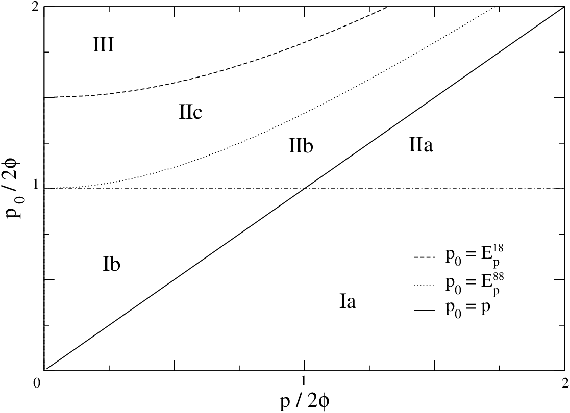
Below the light cone, p0<pp_{0}<p, the imaginary part of the HDL electric and magnetic gluons is nonzero, cf. Fig.(1) of Ref. [22]. Hence, the gluons are Landau damped. This is equivalent to regions Ia and IIa of Fig. (1) of this paper. In these regions, then, the spectral densities are calculated from Eq. (50). However, above the light cone, p0>pp_{0}>p, regions IIb, IIc, and III, the imaginary parts are zero, and therefore, one has to find the spectral densities using Eq. (52). The dispersion relation of the electric and the magnetic gluons in this case are obtained from p0=ω00​(𝐩)p_{0}=\omega_{00}({\bf p}) and p0=ωt​(𝐩)p_{0}=\omega_{t}({\bf p}), respectively. The weak coupling limit, mg≪ϕm_{g}\ll\phi, corresponds to region III of Fig. (1), where ω00​(0)=ωt​(0)=mg\omega_{00}(0)=\omega_{t}(0)=m_{g}.

Refer to caption
Figure 1: Schematic plot of the (p0,p)(p_{0},p) plane. In regions Ia and Ib, the HDL spectral densities are calculated from Eq. (50), and those in the rest of the plane, from Eq. (52). The CFL spectral densities are give by Eq. (50) in regions IIa, IIb, IIc, and III. In regions Ia and Ib, where the light plasmon mode exists, Eq. (52) is used to evaluate the spectral density. Ep18=p2+9​ϕp2{\rm E}^{18}_{p}=\sqrt{p^{2}+9\phi_{p}^{2}} and Ep88=p2+4​ϕp2{\rm E}^{88}_{p}=\sqrt{p^{2}+4\phi_{p}^{2}}, cf. [22].

In the CFL phase, below the light cone and for p0<2​ϕp_{0}<2\phi, region Ia of Fig. (1), the imaginary part of the electric and magnetic gluons are zero; one uses Eq. (52) to find the spectral densities. However, below the light cone and for p0>2​ϕp_{0}>2\phi, the imaginary parts are not zero. This is the case for p0>pp_{0}>p as well. In both of these cases, the spectral densities are obtained from Eq. (50), cf. Ref. [22]. Although the imaginary parts in regions IIb, p<p0<E𝐩88p<p_{0}<E_{\bf p}^{88}, and IIc, E𝐩88<p0<E𝐩18E_{\bf p}^{88}<p_{0}<E_{\bf p}^{18}, are approximately at order of the HDL limit, they are very small in region III, p0>E𝐩18p_{0}>E_{\bf p}^{18}. In this region Im​Π^00​(p0,𝐩)∼Im​Πt​(p0,𝐩)∼ϕ2{\rm Im}{\hat{\Pi}}_{00}(p_{0},{\bf p})\sim{\rm Im}\Pi_{t}(p_{0},{\bf p})\sim\phi^{2}.

The Nambu-Goldstone (NG) bosons appear in region Ia, cf. Ref. [22]. The light plasmon modes, however, are present in regions Ia and Ib. In these regions, as stated before, the imaginary parts of the color-superconducting gluon self-energy are zero and the gluon energy and momentum are much smaller than the gap. The dispersion relation of the NG bosons is evaluated from Pμ​Pν​Πμ​ν​(P)=0P_{\mu}P_{\nu}\Pi^{\mu\nu}(P)=0 and that for the light plasmons is calculated from Eq. (52). In this regime, p0,p≪ϕp_{0},p\ll\phi, the dispersion relation is approximately linear. Hence, we can expand the self-energies in terms of its momentum and energy. The leading terms are

Π00​(p0,𝐩)\displaystyle\Pi^{00}(p_{0},{\bf p}) ≃\displaystyle\simeq mg23​(2.6+0.4​p02ϕ2),\displaystyle\frac{m_{g}^{2}}{3}\left(2.6+0.4\,\frac{p_{0}^{2}}{\phi^{2}}\right)\,, (61a)
Πℓ​(p0,𝐩)\displaystyle\Pi^{\ell}(p_{0},{\bf p}) ≃\displaystyle\simeq mg210​p02ϕ2,\displaystyle\frac{m_{g}^{2}}{10}\,\frac{p_{0}^{2}}{\phi^{2}}\,, (61b)
Π0​i​(p0,𝐩)​p^i\displaystyle\Pi^{0i}(p_{0},{\bf p}){\hat{p}}^{i} ≃\displaystyle\simeq −mg2150​pϕ​p02ϕ2,\displaystyle-\frac{m_{g}^{2}}{150}\,\frac{p}{\phi}\,\frac{p_{0}^{2}}{\phi^{2}}\,, (61c)
Πt​(p0,𝐩)\displaystyle\Pi^{t}(p_{0},{\bf p}) ≃\displaystyle\simeq mg220​(1−3​p02ϕ2),\displaystyle\frac{m_{g}^{2}}{20}\left(1-3\,\frac{p_{0}^{2}}{\phi^{2}}\right)\,, (61d)

where the explicit forms of the self-energies are taken from Eq. (A2) of Ref. [22]. We refrain from presenting the details of the calculations leading to Eq. (61). Similar calculations for the 2SC phase are done in Ref. [27]. In this limit, the longitudinal self-energy Π^00​(p0,𝐩){\hat{\Pi}}^{00}(p_{0},{\bf p}) [cf. Eq.(4b) of Ref. [22]] is given by

Π^00​(p0,𝐩)≃mg210​p2ϕ2​(1+0.2​p02ϕ2).\displaystyle{\hat{\Pi}}^{00}(p_{0},{\bf p})\simeq\frac{m_{g}^{2}}{10}\,\frac{p^{2}}{\phi^{2}}\left(1+0.2\,\frac{p_{0}^{2}}{\phi^{2}}\right)\,. (62)

Having calculated the transverse self-energy in Eq. (61), the magnetic gluon propagator, Δt​(P)=1/(p02−p2−Πt​(P))\Delta^{t}(P)=1/(p_{0}^{2}-p^{2}-\Pi^{t}(P)) becomes

[Δt​(P)]−1≃[p02​(1+320​mg2ϕ2)−𝐩2−mg220].\displaystyle\left[\Delta^{t}(P)\right]^{-1}\simeq\left[p_{0}^{2}\left(1+\frac{3}{20}\frac{m_{g}^{2}}{\phi^{2}}\right)-{\bf p}^{2}-\frac{m_{g}^{2}}{20}\right]\,. (63)

The light plasmon dispersion relation, therefore, reads

ωt≃203​ϕmg​p2+mg220.\displaystyle\omega_{t}\simeq\sqrt{\frac{20}{3}}\frac{\phi}{m_{g}}\sqrt{p^{2}+\frac{m_{g}^{2}}{20}}\,. (64)

Employing this and Eq. (63) in Eq. (53) one can find the associated residue

𝒵t​(𝐩)≃53​ϕmg​p.\displaystyle\mathcal{Z}_{t}({\bf p})\simeq\sqrt{\frac{5}{3}}\frac{\phi}{m_{g}p}\,. (65)

We will make use of this result in Sec. III.3.

In the next section we estimate the effect of the gluon self-energy on the value of the gap. For that, we have to investigate the spectral densities in the HDL limit as well as in the color-superconducting phase, cf. Equation (58).

III Results

In this section, I estimate the values of ℐ00​(ω)\mathcal{I}_{00}(\omega) and ℐt​(ω)\mathcal{I}_{t}(\omega) to find the effects of the self-energy on the value of the gap.

III.1 Estimate for ℐ00​(ω)\mathcal{I}_{00}(\omega)

The qualitative results of this part are very similar to those of the 2SC phase for ℐ0011​(ω)\mathcal{I}_{00}^{11}(\omega) in Ref. [7], except that region IIc in Fig. (1) is new for the CFL phase. For p0<2​ϕp_{0}<2\phi, the spectral densities of the CFL phase are zero for both regions Ia and Ib, ρ00=0\rho_{00}=0, cf. Fig.(3) of [22]. For the HDL limit, above the light cone, in region Ib, the spectral density is zero, therefore δ​ρ00=0\delta\rho_{00}=0. However, in region Ia, the HDL spectral density is regular and we have δ​ρ00=−ρ00HDL\delta\rho_{00}=-\rho_{00}^{\rm HDL}. In this case, the spectral density is given by

ρ00HDL​(ω,p)=θ⁡(p−ω)​mg2​ωp​{[p2+2​mg2​(1−ω2​p​ln​|p+ωπ−ω|)]2+(π​mg2​ωp)2}−1,\displaystyle\rho_{00}^{\rm HDL}(\omega,p)=\theta(p-\omega)m_{g}^{2}\frac{\omega}{p}\left\{\left[p^{2}+2\,m_{g}^{2}\left(1-\frac{\omega}{2p}{\rm ln}\left|\frac{p+\omega}{\pi-\omega}\right|\right)\right]^{2}+\left(\pi m_{g}^{2}\frac{\omega}{p}\right)^{2}\right\}^{-1}\,, (66)

where mgm_{g} is the gluon mass at zero temperature, mg2=g2​μ2/2​π2m_{g}^{2}=g^{2}\mu^{2}/2\pi^{2}. For pp at order of ω\omega, the HDL spectral density, Eq. (66), is approximately zero and for p≫ωp\gg\omega it is of order ∼1/p5\sim 1/p^{5}. Therefore, using Eq. (58) we have

ℐ00​(ω)∼ωmg∼ϕmg.\displaystyle\mathcal{I}_{00}(\omega)\sim\frac{\omega}{m_{g}}\sim\frac{\phi}{m_{g}}\,. (67)

Here, we neglected powers of gg because they do not have any consequence on the order of ℐ00​(ω)\mathcal{I}_{00}(\omega), cf.[7]. The effect of color superconductivity, however, appears for p0>2​ϕp_{0}>2\phi. In region IIa, both ρ00\rho_{00} and ρ00HDL\rho^{\rm HDL}_{00} are regular. Since for ϕ→0\phi\rightarrow 0 we recover the normal phase, δ​ρ00→0\delta\rho_{00}\rightarrow 0 (cf. Ref. [22]), to leading we have

∫ω2​μd​p​p​δ​ρ00​(ω,p)∼ϕmg.\displaystyle\int_{\omega}^{2\mu}dp\,p\,\delta\rho_{00}(\omega,p)\sim\frac{\phi}{m_{g}}\,. (68)

On the other hand, in regions IIb and IIc, the HDL spectral densities are zero and ρ00\rho_{00} is of order 1/mg21/m_{g}^{2}. Then, for region IIb

∫ω2−4​ϕ2ωd​p​p​δ​ρ00​(ω,p)∼ϕ2mg2,\displaystyle\int_{\sqrt{\omega^{2}-4\,\phi^{2}}}^{\omega}dp\,p\,\delta\rho_{00}(\omega,p)\sim\frac{\phi^{2}}{m_{g}^{2}}\,, (69)

and for region IIc

∫ω2−9​ϕ2ω2−4​ϕ2d​p​p​δ​ρ00​(ω,p)∼ϕ2mg2.\displaystyle\int_{\sqrt{\omega^{2}-9\,\phi^{2}}}^{\sqrt{\omega^{2}-4\,\phi^{2}}}dp\,p\,\delta\rho_{00}(\omega,p)\sim\frac{\phi^{2}}{m_{g}^{2}}\,. (70)

In region III, the spectral density for the CFL phase is a smeared delta function and that for the HDL limit is a true one. Nevertheless, the integral over momentum in Eq. (58) makes ℐ00​(ω)\mathcal{I}_{00}(\omega) regular. Qualitatively, the argument used for region IIa is valid at this region too. When ϕ→0\phi\rightarrow 0 we have ρ00≃ρ00HDL\rho_{00}\simeq\rho_{00}^{\rm HDL}, hence,

∫0ω2−9​ϕ2d​p​p​δ​ρ00​(ω,p)∼ϕmg.\displaystyle\int_{0}^{\sqrt{\omega^{2}-9\,\phi^{2}}}dp\,p\,\delta\rho_{00}(\omega,p)\sim\frac{\phi}{m_{g}}\,. (71)

In conclusion, ℐ00​(ω)\mathcal{I}_{00}(\omega) is at most of order ϕ/mg\phi/m_{g}.

III.2 Estimate for ℐt​(ω)\mathcal{I}_{t}(\omega)

The arguments used in the previous section for regions where p0>2​ϕp_{0}>2\phi are valid for ℐt​(ω)\mathcal{I}_{t}(\omega) too. However, for p0<2​ϕp_{0}<2\phi, the scenario is different because the light plasmon modes appear in the regions Ia and Ib. In these regions, since the imaginary parts of the gluon self-energy are zero, one has to use Eq. (52) to find the associated spectral densities. For both of these regions, the color-superconducting contribution is

∫ω2​μd​p​p​ρt​(ω,p)=−p⁡(ωt)​𝒵t​(p)​(|∂ωt​(p)∂p|)p=p⁡(ωt)−1\displaystyle\int_{\omega}^{2\mu}dp\,p\,\rho_{t}(\omega,p)=-p(\omega_{t})\mathcal{Z}_{t}(p)\left(\left|\frac{\partial\,\omega_{t}(p)}{\partial\,p}\right|\right)^{-1}_{p=p(\omega_{t})} (72)

Making use of Eqs. (64) and (65) in Eq. (72) yields

∫ω2​μd​p​p​ρt​(ω,p)≃−1.\displaystyle\int_{\omega}^{2\mu}dp\,p\,\rho_{t}(\omega,p)\simeq-1\,. (73)

In region Ia, one can approximate the HDL spectral density for p≫ωp\gg\omega as

ρtHDL​(ω,p)≃θ⁡(p−ω)​mg2​ω​pp6+(π​mg2​ω)2.\displaystyle\rho_{t}^{\rm HDL}(\omega,p)\simeq\theta(p-\omega)\,m_{g}^{2}\,\frac{\omega\,p}{p^{6}+(\pi\,m_{g}^{2}\,\omega)^{2}}\,. (74)

This gives rise to

∫ω2​μd​p​p​ρtHDL​(ω,p)≃ϕmg.\displaystyle\int_{\omega}^{2\mu}dp\,p\,\rho_{t}^{\rm HDL}(\omega,p)\simeq\frac{\phi}{m_{g}}\,. (75)

Therefore in this region, to leading order, ℐt​(ω)\mathcal{I}_{t}(\omega) is at most of order one,

ℐt​(ω)=∫ω2​μd​p​p​δ​ρt​(ω,p)∼−1.\displaystyle\mathcal{I}_{t}(\omega)=\int_{\omega}^{2\mu}dp\,p\,\delta\rho_{t}(\omega,p)\sim-1\,. (76)

Furthermore, since in region Ib the HDL spectral density vanishes whereas the light plasmon spectral density persist, ℐt​(ω)\mathcal{I}_{t}(\omega) is of order ∼1\sim 1 too.

As mentioned, for the other regions, p0>2​ϕp_{0}>2\phi, ℐt​(ω)\mathcal{I}_{t}(\omega) has the same order of magnitude as ℐ00​(ω)\mathcal{I}_{00}(\omega), namely, it is at most of order ∼ϕ/mg\sim\phi/m_{g}. In the next section, we take into account these effects on the value of the gap.

III.3 Estimate for δ​ϕk\delta\phi_{k}

Having estimated the order of ℐ00​(ω)\mathcal{I}_{00}(\omega) and ℐt​(ω)\mathcal{I}_{t}(\omega) we can now estimate the effect of the gluon self-energy on the gap. For p0<2​ϕp_{0}<2\phi, ℐ00​(ω)\mathcal{I}_{00}(\omega) is at most of order ∼ϕ/mg\sim\phi/m_{g} and ℐt​(ω)\mathcal{I}_{t}(\omega) of order ∼1\sim 1. As mentioned earlier, we do not take into account the additional powers of the coupling gg, because they are always accompanied by at least one power of the gap which is exponentially small in gg, ϕ∼exp(−1/g)\phi\sim\exp(-1/g). Employing Eq. (76) in Eq. (60), after performing the ω\omega integral, we have

δϕk∼−g2∫μ−δμ+δdqϕqϵ𝐪ln|(2​ϕ+ϵ𝐪)2−ϵ𝐤2ϵ𝐪2−ϵ𝐤2|,\displaystyle\delta\phi_{k}\sim-g^{2}\int_{\mu-\delta}^{\mu+\delta}dq\,\frac{\phi_{q}}{\epsilon_{{\bf q}}}\,{\rm ln}\left|\frac{(2\phi+\epsilon_{{\bf q}})^{2}-\epsilon_{{\bf k}}^{2}}{\epsilon_{{\bf q}}^{2}-\epsilon_{{\bf k}}^{2}}\right|\,, (77)

In Appendix B of Ref.[7] it is shown that this integral has a positive value and is at most of order ∼ϕ\sim\phi. Therefore, δ​ϕk\delta\phi_{k} contributes to the O⁡(g)O(g) of the gap in Eq. (4), i.e. to the subsubleading order. Thus, the coefficients bb and cc are not modified. In addition, since δ​ϕk\delta\phi_{k} has a negative sign, the effect of the gluon self-energy is to decrease the value of the gap. This is in agreement with the previous result obtained using the Ginzburg-Landau theory, which shows near the critical temperature TcT_{c} the CFL gluon self-energy decreases the value of the gap [28].

IV Conclusion

In conclusion, in the weak coupling limit, we studied the effect of CFL gluon self-energy on the solution of the gap. For the values of the energy and momentum, where the spectral densities of the the CFL color superconductivity are regular, the effect of the gluon self-energy is very negligible, i.e. it does not even appear up to subsubleading order. However, for the energies and momenta, where the light plasmon mode appears, the effect is of subsubleading order.

V Acknowledgments

The author thanks Owe Philipsen for fruitful discussions and also Institute for Theoretische Physik of Muenster University for financial support.

References

  • [1] D. Bailin and A. Love, Phys. Rep. 107 (1984) 325.
  • [2] D. J. Gross and F. Wilczek, Phys. Rev. Lett. 30 (1973) 1343 (1973); H. D. Politzer, Phys. Rev. Lett. 30 (1973) 1346.
  • [3] J. R. Schrieffer, Theory of Superconductivity (New York, W.A. Benjamin, 1964).
  • [4] A. L. Fetter and J. D. Walecka, Quantum Theory of Many-Particle Systems (McGraw–Hill, New York, 1971); A. A. Abrikosov, L. P. Gorkov, and I. E. Dzyaloshinski, Methods of Quantum Field Theory in Statistical Physics (Dover, New York, 1963).
  • [5] R. D. Pisarski and D.H. Rischke, Phys. Rev. D60 (1999) 094013.
  • [6] R. D. Pisarski and D.H. Rischke, Phys. Rev. D61 (2000), 051501; Phys. Rev. D61 (2000), 074017.
  • [7] D. H. Rischke, Phys. Rev. D64 (1999) 094003.
  • [8] D. T. Son, Phys. Rev. D59 (1999) 094019.
  • [9] T. Schäfer and F. Wilczek, Phys. Rev. D60 (1999) 114033.
  • [10] D. K. Hong, V. A. Miransky, I. A. Shovkovy, and L. C. R. Wijewardhana, Phys. Rev. D61 (2000) 056001.
  • [11] S. D. H. Hsu, and M. Schwetz, Nucl. Phys. B572 (2000) 211.
  • [12] W. E. Brown, J. T. Liu, and H.-C. Ren, Phys. Rev. D61 (2000) 114012; 62 (2000) 054013, 054016.
  • [13] S. R. Beane, P. F. Bedaque, and M. J. Savage, Phys. Lett. B483 (2000) 131; Nucl. Phys. A688 (2001) 931.
  • [14] B. C. Barrois, PhD thesis, report UMI 79-04847 (1979).
  • [15] M. Le Bellac, Thermal Field Theory (Cambridge, Cambridge University Press, 1996).
  • [16] J.-P. Blaizot and J.-Y. Ollitrault, Phys. Rev. D48 (1993) 1390; H. Vija and M. H. Thoma, Phys. Lett. B342 (1995) 212; C. Manuel, Phys. Rev. D53 (1996) 5866.
  • [17] C. Manuel, Phys. Rev. D 62 (2000) 114008; Qun Wang, D. H. Rischke, Phys. Rev. D65 (2002) 054005.
  • [18] A. Schmitt,, Q. Wang, and D. H. Rischke, Phys.Rev. D66 (2002) 114010; A. Schmitt, Phys. Rev. D71 (2005) 054016.
  • [19] Hao-jie Xu and Qun Wang, [0810.2168].
  • [20] D. H. Rischke, Phys. Rev. D62 (2000) 054017.
  • [21] D. H. Rischke, Phys. Rev. D62 (2000) 034007.
  • [22] H. Malekzadeh, D. H. Rischke, Phys. Rev. D73 (2006) 114006.
  • [23] K. Zarembo, Phys. Rev. D62 (2000) 054003; I. A. Shovkovy and L. C. R. Wijewardhana, Phys. Lett. B470 (1999) 189.
  • [24] D. J. Gross, R. D. Pisarski, and L. G. Yaffe, Rev. Mod. Phys. 53 (1981) 43;
  • [25] R. D. Pisarski, Physica A 158 (1989) 146.
  • [26] I. A. Shovkovy and L. C. R. Wijewardhana, Phys. Lett. B 470 (1999) 189; T. Schäfer, Nucl. Phys. B 575 (2000) 269.
  • [27] D. H. Rischke, D. T. Son, and M. A. Stephanov, Phys. Rev. Lett. 87 (2001) 062001.
  • [28] Kei Iida, Phys. Rev. D72 (2005) 054025.