A non-negative expansion for small Jensen-Shannon Divergences

Anil Raj Affiliation: Department of Applied Physics and Applied Mathematics
Columbia University, New York Email: ar2384@columbia.edu Chris H. Wiggins Affiliation: Department of Applied Physics and Applied Mathematics
Center for Computational Biology and Bioinformatics
Columbia University, New York Email: chris.wiggins@columbia.edu

August 24, 2026

Abstract

In this report, we derive a non-negative series expansion for the Jensen-Shannon divergence (JSD) between two probability distributions. This series expansion is shown to be useful for numerical calculations of the JSD, when the probability distributions are nearly equal, and for which, consequently, small numerical errors dominate evaluation.

Keywords:

entropy, JS divergence

I Introduction

The Jensen-Shannon divergence (JSD) has been widely used as a dissimilarity measure between weighted probability distributions. The direct numerical evaluation of the exact expression for the JSD (involving difference of logarithms), however, leads to numerical errors when the distributions are close to each other (small JSD); when the element-wise difference between the distributions is $O(10^{-1})$ , this naive formula produces erroneous values (sometimes negative) when used for numerical calculations. In this report, we derive a provably non-negative series expansion for the JSD which can be used in the small JSD limit, where the naive formula fails.

II Series expansion for Jensen-Shannon divergence

Consider two discrete probability distributions ${\bf{p}}_{1}$ and ${\bf{p}}_{2}$ over a sample space ${\bf{S}}$ of cardinality $N$ with relative normalized weights $\pi_{1}$ and $\pi_{2}$ between them. The JSD between the distributions is then defined as [1]

\displaystyle\Delta_{naive}[{\bf{p}}_{1},{\bf{p}}_{2};\pi_{1},\pi_{2}]=H[\pi_{1}{\bf{p}}_{1}+\pi_{2}{\bf{p}}_{2}]-(\pi_{1}H[{\bf{p}}_{1}]+\pi_{2}H[{\bf{p}}_{2}])

(1)

where the entropy (measured in nats) of a probability distribution is defined as

\displaystyle H[{\bf{p}}]=-\sum_{j=1}^{N}h(p_{j})=-\sum_{j=1}^{N}p_{j}\log(p_{j}).

(2)

Defining

\displaystyle\begin{matrix}\bar{p}_{j}&=&({p_{1j}+p_{2j}})/{2}&;&0\leqslant\bar{p}_{j}\leqslant 1&;\sum_{j=1}^{N}\bar{p}_{j}=1\\ \eta_{j}&=&({p_{1j}-p_{2j}})/{2}&;&\sum_{j=1}^{N}\eta_{j}=0&\\ \varepsilon_{j}&=&({\eta_{j}})/{\bar{p}_{j}}&;&-1\leqslant\varepsilon_{j}\leqslant 1&\\ \alpha&=&\pi_{1}-\pi_{2}&;&-1\leqslant\alpha\leqslant 1&\end{matrix}

(3)

we have

	$\displaystyle h(\pi_{1}p_{1j}+\pi_{2}p_{2j})$	$\displaystyle=$	$\displaystyle-(\pi_{1}(\bar{p}_{j}+\eta_{j})+\pi_{2}(\bar{p}_{j}-\eta_{j}))\log(\pi_{1}(\bar{p}_{j}+\eta_{j})+\pi_{2}(\bar{p}_{j}-\eta_{j}))$		(4)
		$\displaystyle=$	$\displaystyle-\bar{p}_{j}(1+\alpha\varepsilon_{j})\left[\log(\bar{p}_{j})+\log(1+\alpha\varepsilon_{j})\right]$		(4)

and

$\displaystyle\pi_{1}h(p_{1j})+\pi_{2}h(p_{2j})$	$\displaystyle=$	$\displaystyle-\pi_{1}(\bar{p}_{j}+\eta_{j})\log(\bar{p}_{j}+\eta_{j})-\pi_{2}(\bar{p}_{j}-\eta_{j})\log(\bar{p}_{j}-\eta_{j})$	(5)
	$\displaystyle=$	$\displaystyle-\frac{1}{2}\bar{p}_{j}(1+\alpha)(1+\varepsilon_{j})\log(\bar{p}_{j}(1+\varepsilon_{j}))-\frac{1}{2}\bar{p}_{j}(1-\alpha)(1-\varepsilon_{j})\log(\bar{p}_{j}(1-\varepsilon_{j}))$
	$\displaystyle=$	$\displaystyle-\bar{p}_{j}(1+\alpha\varepsilon_{j})\log(\bar{p}_{j})-\frac{1}{2}\bar{p}_{j}(1+\alpha\varepsilon_{j})\log(1-\varepsilon_{j}^{2})-\frac{1}{2}\bar{p}_{j}(\alpha+\varepsilon_{j})\log\left(\frac{1+\varepsilon_{j}}{1-\varepsilon_{j}}\right).$

Thus,

\displaystyle h(\pi_{1}p_{1j}+\pi_{2}p_{2j})-(\pi_{1}h(p_{1j})+\pi_{2}h(p_{2j}))

\displaystyle=

\displaystyle\frac{1}{2}\bar{p}_{j}\left[(1+\alpha\varepsilon_{j})\log\left(\frac{1-\varepsilon_{j}^{2}}{(1+\alpha\varepsilon_{j})^{2}}\right)+(\alpha+\varepsilon_{j})\log\left(\frac{1+\varepsilon_{j}}{1-\varepsilon_{j}}\right)\right].

(6)

The Taylor series expansion of the logarithm function is given as

\displaystyle\log(1+x)=\sum_{i=1}^{\infty}c_{i}x^{i};~~~c_{i}=\frac{(-1)^{i+1}}{i}.

(7)

The logarithms in the expression for the J-S divergence can then be written as

$\displaystyle\log(1+\varepsilon_{j})$	$\displaystyle=$	$\displaystyle\sum_{i=1}^{\infty}c_{i}\varepsilon_{j}^{i}$
$\displaystyle\log(1-\varepsilon_{j})$	$\displaystyle=$	$\displaystyle\sum_{i=1}^{\infty}(-1)^{i}c_{i}\varepsilon_{j}^{i}$	(8)
$\displaystyle\log(1+\alpha\varepsilon_{j})$	$\displaystyle=$	$\displaystyle\sum_{i=1}^{\infty}c_{i}\alpha^{i}\varepsilon_{j}^{i}.$

We then have $\Delta=\frac{1}{2}\sum_{j=1}^{N}\bar{p}_{j}\delta_{j}$ , with

$\displaystyle\delta_{j}$	$\displaystyle=$	$\displaystyle(1+\alpha\varepsilon_{j})\left[\log(1+\varepsilon_{j})+\log(1-\varepsilon_{j})-2\log(1+\alpha\varepsilon_{j})\right]+(\alpha+\varepsilon_{j})\left[\log(1+\varepsilon_{j})-\log(1-\varepsilon_{j})\right]$	(9)
	$\displaystyle=$	$\displaystyle(1+\alpha\varepsilon_{j})\left[\sum_{i=1}^{\infty}c_{i}\varepsilon_{j}^{i}+\sum_{i=1}^{\infty}(-1)^{i}c_{i}\varepsilon_{j}^{i}-2\sum_{i=1}^{\infty}c_{i}\alpha^{i}\varepsilon_{j}^{i}\right]+(\alpha+\varepsilon_{j})\left[\sum_{i=1}^{\infty}c_{i}\varepsilon_{j}^{i}-\sum_{i=1}^{\infty}(-1)^{i}c_{i}\varepsilon_{j}^{i}\right]$
	$\displaystyle=$	$\displaystyle\sum_{i=1}^{\infty}c_{i}\left[\varepsilon_{j}^{i}+\alpha\varepsilon_{j}^{i+1}+(-1)^{i}\varepsilon_{j}^{i}+(-1)^{i}\alpha\varepsilon_{j}^{i+1}-2\alpha^{i}\varepsilon_{j}^{i}-2\alpha^{i+1}\varepsilon_{j}^{i+1}+\alpha\varepsilon_{j}^{i}+\varepsilon_{j}^{i+1}+(-1)^{i+1}\alpha\varepsilon_{j}^{i}+(-1)^{i+1}\varepsilon_{j}^{i+1}\right]$
	$\displaystyle=$	$\displaystyle\sum_{i=1}^{\infty}c_{i}\left[\left\{(-1)^{i}-2\alpha^{i}+\alpha+(-1)^{i+1}\alpha+1\right\}\varepsilon_{j}^{i}+\left\{(-1)^{i}\alpha-2\alpha^{i+1}+1+(-1)^{i+1}+\alpha\right\}\varepsilon_{j}^{i+1}\right].$

When $i=1$ , ${\rm coeff}(\varepsilon_{j})=c_{1}(-1-2\alpha+\alpha+\alpha+1)=0$ . The first non-vanishing term in the expansion is then of order 2. Shifting indices of the first term in Eqn. (9) gives

$\displaystyle\delta_{j}$	$\displaystyle=$	$\displaystyle\sum_{i=1}^{\infty}\left[c_{i+1}\left\{(-1)^{i+1}-2\alpha^{i+1}+\alpha+(-1)^{i+2}\alpha+1\right\}+c_{i}\left\{(-1)^{i}\alpha-2\alpha^{i+1}+1+(-1)^{i+1}+\alpha\right\}\right]\varepsilon_{j}^{i+1}$	(10)
	$\displaystyle=$	$\displaystyle\sum_{i=1}^{\infty}(c_{i}+c_{i+1})\left\{(-1)^{i}\alpha-2\alpha^{i+1}+\alpha+1+(-1)^{i+1})\right\}\varepsilon_{j}^{i+1}$
	$\displaystyle=$	$\displaystyle\sum_{i=1}^{\infty}\frac{(-1)^{i+1}}{i(i+1)}\left\{(-1)^{i}\alpha-2\alpha^{i+1}+\alpha+1+(-1)^{i+1})\right\}\varepsilon_{j}^{i+1}$
	$\displaystyle=$	$\displaystyle\sum_{i=1}^{\infty}B_{i}\varepsilon_{j}^{i+1}$

where

\displaystyle B_{i}

\displaystyle=

\displaystyle\frac{1-\alpha+(-1)^{i+1}(1+\alpha-2\alpha^{i+1})}{i(i+1)}=\Biggl\{\begin{matrix}{2(1-\alpha^{i+1})}/\left({i(i+1)}\right)&i~{\rm odd},\cr{-2(\alpha-\alpha^{i+1})}/\left({i(i+1)}\right)&i~{\rm even.}\end{matrix}

(11)

This series expansion can be further simplified as

$\displaystyle\delta_{j}$	$\displaystyle=$	$\displaystyle\sum_{i=1}^{\infty}\left(B_{2i-1}+B_{2i}\varepsilon_{j}\right)\varepsilon_{j}^{2i}$	(12)
	$\displaystyle=$	$\displaystyle\sum_{i=1}^{\infty}B_{2i-1}\left(1+\frac{B_{2i}}{B_{2i-1}}\varepsilon_{j}\right)\varepsilon_{j}^{2i},$	(12)
$\displaystyle\frac{B_{2i}}{B_{2i-1}}\varepsilon_{j}$	$\displaystyle=$	$\displaystyle-\left(\frac{2i-1}{2i+1}\right)\alpha\varepsilon_{j}.$	(13)

Since $-1\leqslant\alpha\varepsilon_{j}\leqslant 1$ , we have $-1\leqslant\frac{B_{2i}}{B_{2i-1}}\varepsilon_{j}\leqslant 1$ . Thus, for every $i$ , $(B_{2i-1}+B_{2i}\varepsilon_{j})\varepsilon_{j}^{2i}\geqslant 0$ , making $\delta_{j}$ — and the series expansion for $\Delta_{naive}$ — non-negative up to all orders.

III Numerical Results

The accuracy of the truncated series expansion can be compared with the naive formula by measuring the JSD between randomly generated probability distributions. Pairs of probability distributions with $-4\leqslant\log_{10}\|{\bf{\varepsilon}}\|<0$ , where $\|{\bf{\varepsilon}}\|=\sqrt{\frac{\sum_{j=1}^{N}\varepsilon_{j}^{2}}{N}}$ , were randomly generated and the J-S divergence between each pair was calculated by both a direct evaluation of the exact expression ( $\Delta_{naive}$ ) and the approximate expansion ( $\Delta_{k};k\in\{3,6,9,12\}$ ), where

\displaystyle\Delta_{k}=\frac{1}{2}\sum_{j=1}^{N}\bar{p}_{j}\delta_{jk}\quad;\quad\delta_{jk}=\sum_{i=1}^{k}B_{i}\varepsilon_{j}^{i+1}.

(14)

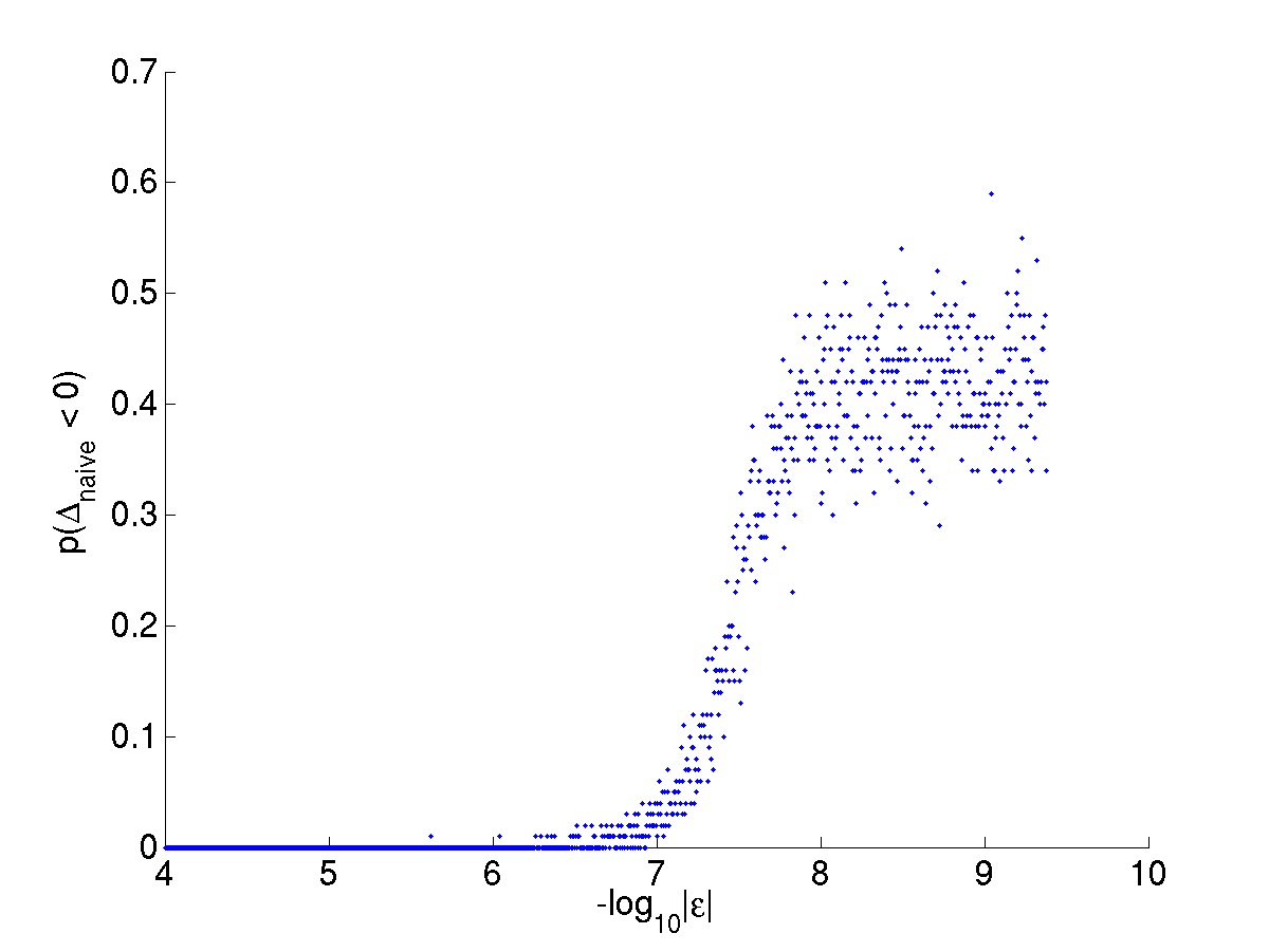
The results shown in Fig. 2 suggest the series expansion to be a more numerically useful formula when the probability distributions differ by $\|{\bf{\varepsilon}}\|\sim O(10^{-0.5})$ . Fig. 2 further shows that when $\|{\bf{\varepsilon}}\|\sim O(10^{-6})$ , a direct evaluation of the exact formula for JSD gives negative values (when implemented in matlab).

Refer to caption — Figure 1: Plot comparing the naive and approximate formulae, truncated at different orders for calculating JSD as a function of the normalized L2-distance ( $\|{\bf{\varepsilon}}\|$ ; see Section III) between pairs of randomly generated probability distributions. Best fit slopes are: -2.05 ( $k=3$ ), -5.89 ( $k=6$ ), -8.14 ( $k=9$ ), -11.91 ( $k=12$ ) and -105.43 (comparing naive with $k=100$ ).

Appendix

Here we include the matlab code used in the figures for approximate evaluation of JSD using its series expansion.


function [JS,epsnorm] = JSapprx(pi1,p1,pi2,p2,order)

% [JS,epsnorm]=JSapprx(pi1,p1,pi2,p2,order) calculates JS
% divergence given two probability distributions and
% their relative weights. JSapprx uses an approximation
% to the JSD by expanding in powers of epsilon=(p1-p2)/(p1+p2)
% and truncating at an order input by the user.
%
% This calculation is described in the technical report
%       ‘‘A non-negative expansion
%       for small Jensen-Shannon Divergences’’
% by Anil Raj and Chris H. Wiggins, October 2008

% average of distributions
pbar=(p1+p2)/2;
% difference of distributions
eta=(p1-p2)/2;
% ratio of difference to average
epsilon=eta./pbar;
% difference in biases, where pi1+pi2=1
alpha=pi1-pi2;

% calculate JS by summing up to order ‘order’
js=zeros(size(pbar));
% denominator computed by summing, as well
denominator=0;
for i=2:order
  denominator=denominator+(i-1);
  % numerical coefficient
  c=(-1)^i*(1/denominator);
  Bi=c*(alpha^(mod(i,2))-alpha^i);
  js=js+Bi*(epsilon.^i);
end

% sum over ‘j’:
JS=pbar’*js/2;

% convert from nats to bits:
JS=JS/log(2);

% norm of epsilon reported as output
if nargout==2
  epsnorm=sqrt(sum(epsilon.^2)/length(pbar));
end

References

[1] J Lin. Divergence measures based on the shannon entropy. IEEE Transactions on Information Theory, 37(1):145–151, Jan 1991.