Quantum site percolation on triangular lattice and the integer quantum Hall effect
Abstract
Generic classical electron motion in a strong perpendicular magnetic field and random potential reduces to the bond percolation on a square lattice. Here we point out that for certain smooth 2D potentials with rotational symmetry this problem reduces to the site percolation on a triangular lattice. We use this observation to develop an approximate analytical description of the integer quantum Hall transition. For this purpose we devise a quantum generalization of the real-space renormalization group (RG) treatment of the site percolation on the triangular lattice. In quantum case, the RG transformation describes the evolution of the distribution of the scattering matrices at the sites. We find the fixed point of this distribution and use it to determine the critical exponent, , for which we find the value . The RG step involves only a single Hikami box, and thus can serve as a minimal RG description of the quantum Hall transition.
pacs
72.15.Rn, 73.20.Fz, 73.43.-fI Introduction
Network-model formulation of the Anderson localization problem was first introduced in Ref. 1. The key observation made in Ref. 1 is that a complex motion of electron in disorder potential can be reduced to the motion along the links of the network (in both directions) with disorder incorporated via random phases of scattering from the nodes of the network. Since then, the network-model approach became a powerful tool for numerical studies of disordered systems. In these studies the randomness is incorporated into the phases accumulated along the network links. A great advantage of the network-model approach to localization is that it can be conveniently applied to various universality classes[2] of disorder. In order to capture the specifics of a given class, one has to impose an appropriate symmetry requirements on the random phases on the links, which fixes the form of -matrix at the nodes. This is achieved by introduction of an internal space associated with the link of the network model, which possesses a desired symmetry. For example, [3] with two-component links (one component for one spin projection) for each direction of propagation the requirements of unitarity and time-reversal symmetry allowed to reveal a delocalization transition expected in two-dimensional systems with spin-orbit scattering. Comprehensive review of the results obtained with the help of the network model is given in Ref. 5. In addition to establishing the existence of localization transitions in different classes, numerical simulations of the network models with the help of transfer-matrix method yields quantitative characteristics of the critical point. These characteristics include critical exponent, critical level statistics, and critical conductance distribution. Corresponding references can be found in the review Ref. 5. Note that, with the exception of Ref. 4 where a particular two-channel network model was considered for arbitrary graph, the underlying network in all previous studies was a square lattice.
Especially convenient for modeling with a network is the chiral motion of a electron in a disorder potential and a strong perpendicular magnetic field. This is because the corresponding network is directed. Directed character of the network with chiral scattering at the nodes allowed Chalker and Coddington [6] to demonstrate conclusively that there is only a single delocalized state per Landau level. This finding is of a great importance, since it is the underlying reason for sharp conductivity peaks at the quantum Hall transition.

On physical grounds, the seminal Chalker-Coddington model [6] of the integer quantum Hall transition can be introduced in a natural way with the help of a two-dimensional potential
| (1) |
In this potential, the equipotential lines form a square lattice. For any nonzero equipotentials are closed. For positive these equipotentials encircle the maxima [and also ] of , while for equipotentials encircle the minima [and ] of . In a strong perpendicular magnetic field 2D electron drifts along equipotentials. Then reconfiguration of equipotentials at , as illustrated in Fig. 1a, manifests the change in the character of motion.
Chalker and Coddington [6] captured the quantum character of motion in by assigning to the saddle points at where the potential behaves as
| (2) | |||
a scattering matrix
Here and are the polar coordinates with origin at , and is the dimensionless energy. For a realistic potential with magnitude, , and correlation length, , dimensionless energy, , is the physical energy measured in the units of the width, , where, , is the magnetic length.

Chalker and Coddington demonstrated that, in order to account for a smooth disorder, it is sufficient to assume that the phases, acquired by a drifting electron between the saddle points, are random.
In this paper we show that the description of the quantum Hall transition can also be obtained based on the potential
| (7) |
which has a triangular symmetry, i.e., and are the basis unit vectors of a triangular lattice; the function is defined inside a “black half” of the rhombus-shape unit cell, see Fig. 2, in the following way
| (8) | |||
Here and are the polar coordinates with respect to the origin at . The form of potential in the “white half” of a unit cell is given by Eq. (7) upon replacement and shifting the origin to the center of the white triangle.
Equipotentials of Eq. (8) evolve, as passes through , in a fashion qualitatively different from the case of quadratic symmetry. As shown in Fig. 1a, in the case of quadratic symmetry, black regions (minima) get connected, while adjacent white regions (maxima) get disconnected. By contrast, the behavior of the potential near the nodes at is given by
| (9) |
where . Corresponding evolution of equipotentials is illustrated in Fig. 1b. We see that, as crosses zero, three black regions get joined at simultaneously. This suggests that quantum mechanical description of motion in the potential requires, in addition to random phases on the links, introducing a scattering matrix at each node. Below we argue that the form of this matrix is
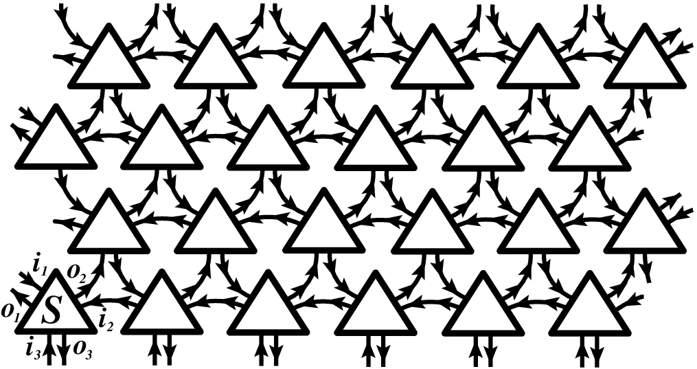
With matrices Eq. (I) in the nodes, the corresponding network model is shown in Fig. 3. In this network the phases on the links are random, as in Chalker-Coddington model, while all -matrices in the nodes, Eq. (I), are the same. As we demonstrate in present paper, this model can be treated numerically using the same MacKinnon-Kramer finite-size scaling algorithm [7] that was employed in Ref. 6 (for subsequent numerical studies of the Chalker-Coddington model see Refs. 8, 9, 10, 11, 12, 13, 14, 15, 16, 17, 18, 19, 20 and review articles [5, 21]).
Chalker-Coddington model can be viewed as quantum version of the classical bond percolation. Establishing one to one correspondence between the classical bonds and the links is possible due to directed character of the chiral CC network. On the other hand, it was demonstrated in Ref. 22 that a simple real-space renormalization group (RG) procedure, based on decimation, leads to the closed equation for the classical bond percolation threshold. This procedure reproduces the exact threshold value and yields a very accurate estimate for the critical exponent. In Refs. 23, 24, 25, 26, 27 the classical RG procedure[22] was generalized to the quantum bond percolation. It was shown that corresponding integral RG equation yields, in addition to the accurate value of the quantum critical exponent, a very accurate distribution of the critical conductance. A real-space RG procedure for a site percolation was proposed in the same paper Ref. 22. This procedure is simpler than for the bond percolation and yields more accurate results. In the present paper this procedure is extended to the quantum case, where it describes the critical behavior of the directed network Fig. 3. As in the classical case, the quantum RG analysis of on the triangular lattice is much easier than the quantum RG analysis of the Chalker-Coddington on the square lattice. This analysis is presented in Sections II-V.
II RG procedure for classical percolation on a triangular network
In order to develop the RG description, it is necessary to incorporate disorder into the -matrices. The reason is that at each RG-step three -matrices, connected by the links, are combined into one super--matrix. Then the randomness in phases translates into the randomness of the elements of super--matrix.
A natural way to devise the quantum RG description is to start from a classical problem of electron drift along the sides of triangles, Fig. 2.
II.1 Classical drift on triangular lattice
Assume that the potential is perturbed near the nodes as
| (16) |
where the random shift, , is much smaller than , but much bigger than the “quantum” energy width, . Depending on the shift, an electron drifting along equipotential towards a node, turns either to the left () or to the right (), see Fig. 1b. We can conventionally call the nodes with and as “black” and “white” lattice sites, respectively. It is obvious that when the average, , is zero, the percolation threshold in the potential Eq. (16) is . In the language of sites, the same is to say that of sites are black at . It is, in fact, well-known [28] that the exact threshold for site percolation on a triangular lattice is . However, it is much less obvious that there is a complete equivalence between electron drift in potential Eq. (16) and the site percolation on a triangular lattice. Superficially, this can be seen from the fact that when two neighboring sites are black, they are connected via the black region. Still, a rigorous proof requires additional steps, in particular, introducing auxiliary hexagons, see Fig. 2. This proof is given in the Appendix A.
II.2 Classical RG scheme
The above mapping on the percolation problem allows one to employ the RG approach to the site percolation on triangular lattice put forward in Ref. 22. This procedure is much simpler than the RG for the bond percolation on the square lattice, proposed in the same paper. Note in passing, that the bond percolation on the square lattice is the classical limit of the Chalker-Coddington model [23].
As shown in Fig. 2, at each RG step [22] the lattice constant increases by a factor of . A site of a rescaled lattice, a supersite, is either black or white depending on the colors of the three constituting sites: if either all three or only two out of three constituting sites are black, then the supersite is black. Otherwise, the supersite is white. Quantitatively, the probability for a supersite to be black is expressed via the corresponding probability for the original site as
| (17) |
Fixed point, , of the transformation Eq. (17) reproduces the exact result . Critical exponent is determined by the condition that the correlation radius, , on the original lattice is equal to the correlation radius on the renormalized lattice, i.e.
| (18) |
Eq. (18) yields , which differs from the exact value, , by only .
The rationale behind the transformation Eq. (17) is that the supersite is located in the center of the black cell in Fig. 2. Then the color of the supersite reflects the “percolation ability” of this black triangular cell, so that, even if one of the nodes, constituting the vertices of the triangular cell is white, the cell still percolates “over black”.
II.3 RG in the language of potential shifts
At this point we make an observation that the above RG procedure can be reformulated in the language of potential with random shifts in the nodes, . Namely, for , , and being the shifts at the nodes constituting a supernode, the shift of the supernode is defined as
| (19) |
where Mid stands for which is smaller than maximal but larger the minimal out of the three numbers. With defined by Eq. (19), the RG equation Eq. (17) describes the evolution of probability that the shift exceeds .
The importance of the above observation is that reformulation of classical RG procedure in terms of potential shifts opens a possibility to capture the quantum-mechanical motion in the random potential. A prescription how to extend classical description to the quantum case is [23]: the algorithm Eq. (19) should be cast in the form of a scattering problem.
III Reformulation in terms of classical transmission
We identify the scattering object as a point where three equipotentials come close as shown in Fig. 4. Incident electron, , either proceeds along the same equipotential into (reflection) or switches equipotentials and proceeds along . Retention of equipotential (reflection) corresponds to positive in the vertex, encircled in Fig. 4. In terms of scattering matrix
the same simple notion can be reformulated as follows. For positive , the matrix is a unit matrix, while for negative the matrix has the form
Superscattering object consists of three scattering objects, and is shown in the same figure.
Now we reformulate Eqs. (17) and (19) in yet another language of -matrices. Namely, the -matrix of a superscattering object is expressed via -matrices of constituting scattering objects upon reducing the number of legs from to . We emphasize that this reduction can be carried out in two distinct ways, as illustrated in Fig. 5. The first way is to perform contractions as , , and . The second variant of contractions is , , and . Now it is straightforward to check that RG transformation Eq. (19) corresponds to the following rule for -matrix of the superscattering object, . If the -matrices of either all three or only two of constituting objects are , then . In all other realizations, when at least two of constituting objects have the matrix , we have .
It is important to note that the above rule for applies independently of the way in which the contractions in Fig. 5 are performed. This is not the case in the quantum version to which we now turn.
IV quantum generalization
Quantum -matrix of the scattering object differs from and in two respects. Firstly, at the points of close contact between each pair of equipotentials electron can switch equipotential even for positive , when it is forbidden classically. Corresponding classically forbidden transitions are illustrated in Fig. 4 with red dashes. Secondly, upon travelling between two subsequent points of close contact, electron accumulates the Aharonov-Bohm phase, . For example, the phase is accumulated in course of drift between and . These phases are irrelevant in the classical limit when the reflection amplitudes, , are either or . However, for intermediate the amplitude for an electron to execute a close contour around the center in Fig. 4 (following the red dashes in the clockwise direction) is finite. As a result, enter into quantum scattering matrix. Explicit form of in terms of and can be obtained by solving three pairs of linear equations, describing quantum scattering at each of three points of the close contact of equipotentials. We have
| (31) | |||
where stand for the transmission amplitudes, and
| (38) |
is the net phase accumulated along the closed contour. It is easy to check that the matrix Eq. (31) is unitary. It is also straightforward to verify that in the classical limits, when all or , Eq. (31) correctly reproduces and , respectively. Detailed derivation of the form Eq. (31) of the scattering matrix is presented in Appendix B.

IV.1 The form of the matrix
From Eq. (31) we can establish the form of the scattering matrix , Eq. (I), with the help of the following duality argument. Due to triangular symmetry of the potential we have . Consider now the transition point, . At this point the probability for electron incident along, say, (see Fig. 4) to be deflected to the left (along ) is equal to the probability to be deflected to the right (along ). Less trivial is that the phase, , must be zero at . This is the consequence of the fact that the scattering problems for electron with energy and are equivalent if we change the drift direction from clockwise to anti-clockwise; this change implies also the change in the sign of .
With , the condition, , of “equal deflection” to the left and to the right, yields a single physical root . Substituting it back in the matrix Eq. (31) reduces it to the scattering matrix Eq. (I) with . Then for probabilities and we get , while the probability is . Including small finite can be also performed with the help of the duality argument, namely that the probability of deflection to the left with energy is equal to the probability of deflection to the right with energy . On the other hand, the change of probability with is .

The role of the matrix is central to the transfer-matrix treatment of the network model; see Appendix C.
IV.2 Quantum RG equation
We now turn to the quantum RG procedure. In contrast to evolution of probability, , upon rescaling of the lattice constant in the classical case, this procedure is formulated in terms of evolution of the distribution function, , of the absolute values of the transmission amplitudes, . Thus the quantum generalization of Eq. (17) at the step is the following recurrence relation
| (39) | |||
The kernel, , represents the conditional probability that, after performing the contractions, the transmission coefficient in Fig. 4 is equal to , provided that the constituting transmission coefficients are , , and , as illustrated in Fig. 4. In analytical evaluation of the dependence it is important to take into account that this dependence is different for two variants of contractions. For a variant , shown in Fig. 5a, the transmission coefficient is given by
| (40) | |||
where is the phase along the contour (), which is now closed. Correspondingly, for the second kind of closing , Fig. 5b, the transmission coefficient has the form
| (41) | |||
where stands for the phase along . For details of derivation of Eqs. (40), (41) see Appendix B.

Relations Eqs. (40), (41) define also the dependencies and . It is important that the central phase, , is common for all three dependencies and . A crucial step in extending classical RG procedure to the quantum case is to follow the ”classical” prescription to choose a middle out of three coefficients
| (42) | |||
and the same for . Eq. (42) is a quantum generalization of the classical Eq. (19). Note that selection of middle value in Eq. (42) is performed for given values of random phases, , , , and . Within RG procedure different phases are uncorrelated, and in evaluation of the kernel we average over each of four phases independently. Finally, taking into account that contractions and are statistically equivalent, the expression for acquires the form
| (43) |
Quantum delocalization corresponds to the fixed point of the transformation Eq. (39). It is found in the next Section.
V Numerical results for fixed point and critical exponent
V.1 The kernel
The examples of the kernel, , calculated using Mathematica from Eqs. (40)-(43), are plotted in Fig. 6 for different sets , , . It is seen that the kernel supports the attractive critical points and . Indeed, for values , the kernel is centered at even smaller value , while for it is around bigger value . In both cases the kernel is narrow. This is because for “classical” transmission coefficients interference does not play a role, so that the phases drop out from Eqs. (40), (41). However, for intermediate values , , the kernel extends over entire interval . It also exhibits peaks at and . The origin of these peaks is the anomalous contributions of phases and to the kernel. Indeed, for these values of phases we have , so that
| (44) | |||
It is easy to check that, when the quadratic form of second derivatives is negatively defined, the corresponding contribution to the kernel is . Therefore, the peaks in the kernel reflect the fact that two loops corresponding to phases and are insufficient for complete averaging. Still, the phase volume of the singular contributions is small, so that the fixed point of the transformation Eq. (39) is not sensitive to these singularities.
V.2 Fixed point
The fixed point, , of the quantum RG equation Eq. (39), satisfies the following nonlinear integral equation
which we have solved using Mathematica. Starting from initial distribution, , and performing analytical fit at each step of successive approximations, the following expression for the fixed point was obtained after the fourth step
| (46) |
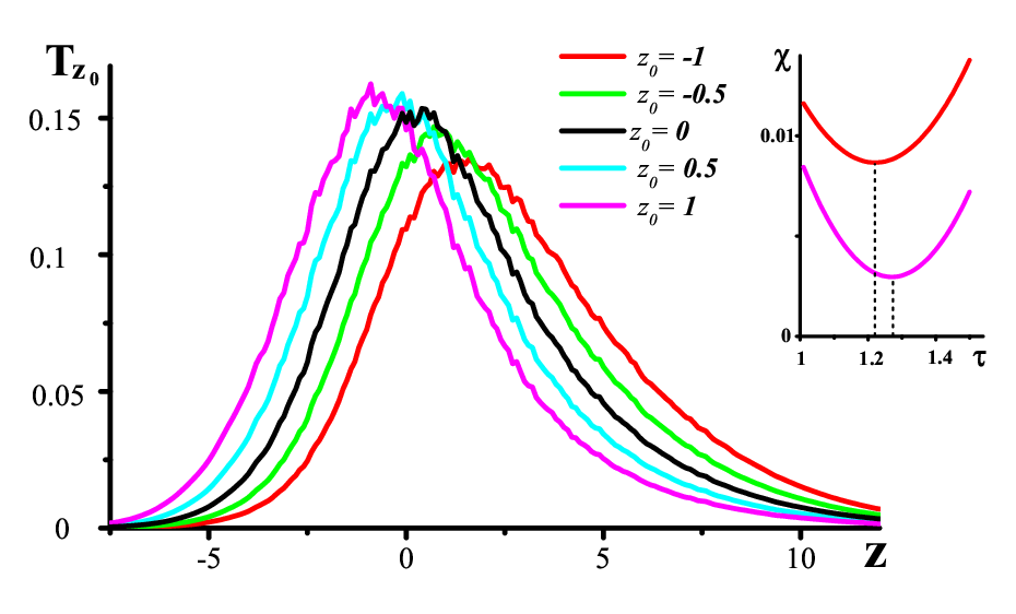
This expression is plotted in Fig. 6b with a green line. One can judge on the accuracy of the approximate solution Eq. (46) by substituting it into the right-hand side of Eq. (V.2). The result, black line in Fig. 6b, is indeed very close to Eq. (46).
The fixed point solution rises upon approaching and . This behavior is inherited from the classical percolation. Note that similar behavior was found in Refs. 23, 25 for the fixed point of the quantum bond percolation on the square lattice. Direct comparison with conductance distribution found in Refs. 23, 25 can be performed using the relation . This comparison indicates that, while numerically the fixed point distributions are close, Eq. (46) favors small values of . Qualitatively, this reflects the fact that at critical energy, , electron incident along (see Fig. 4) is more likely to proceed along rather than switch to . The asymmetry is seen more clearly if one interprets in terms of distribution, of heights of the effective saddle point. This height is determined by the relation , so that
| (47) |
The distribution is shown in Fig. 7 with a black line. It has an asymmetry towards large .
V.3 Critical exponent
To estimate the critical exponent, , which governs the divergence of localization radius, , as a function of energy, , we used the reasoning from Refs. 23, 25. Electron with finite energy, , “sees” the shifted distribution of the saddle point heights , where is proportional to . The key step of the reasoning [23, 25] is that, upon the RG transformation, the electron travels on the lattice with the lattice constant and sees the shifted distribution of heights, , where is some constant independent of . After subsequent RG steps this distribution evolves into . When the shift accumulates to reach , the electron becomes localized within the size of a unit cell of renormalized lattice. Then from the relations
| (48) |
we find
| (49) |
This definition of is a quantum generalization of Eq. (18). In Fig. 7 the result of calculation for four , , , is shown. We see that for these the shape of is only slightly affected by the shift. The curves are approximately equidistant, so that an estimate of can be obtained simply from the horizontal separation between the neighboring curves. This yields and, correspondingly, . For more accurate estimate we studied the variance,
| (50) |
as a function of for different values of the “energy shift” . The sum Eq. (50) was taken over discrete set for . In Fig. 7 we plot the variance for and . Both curves have pronounced minima at and , respectively. This translates into the values of and . Although these values are in good agreement with known value of , the accuracy of the above estimate is limited. The limitation is due to the fact that for the heights of maxima of the curves , shown in Fig. 7, differ from the height of . This deviation would not be a problem for smaller . However for the variance becomes small, and its dependence on becomes weak. Apparently, the variance Eq. (50) is affected by the wiggles at the top of the curves much stronger for than for , which makes the evaluation of for small ineffective.
VI conclusion
It is interesting to point out that, while the classical limit of the Chalker-Coddington model based on potential Eq. (2) reduces to the bond percolation, similar form of potential Eq. (16) leads to the site percolation. The reason is the symmetry of corresponding potentials. As seen from Fig. 2, the hexagons surrounding the nodes of potential Eq. (16) have common sides. On the other hand, the squares, drawn around the nodes of potential Eq. (2) share the vertices.
Both the bond percolation on a square lattice and the site percolation on triangular lattice have , which is insured by self-duality. The RG descriptions [22] of both cases, having fixed point, , effectively preserve this self-duality. As a result, the RG values for classical exponent come out close to in both RG schemes. In this paper we demonstrated that quantum extension of classical RG to the triangular lattice also yields the critical exponent close to the known value .
The fact that the simple RG scheme, considered in the present paper, describes the quantum Hall transition so accurately has a deep underlying reason. Delocalized state in the quantum Hall transition emerges as a result of competition of two trends: (i) quantum interference processes that survive in the presence of magnetic field (Hikami boxes, Ref. 29) tend to localize electron, while (ii) classical Lorentz force, by causing electron drift, prevents it from repeating closed diffusive trajectories. Both trends are incorporated into our RG scheme. Obviously, chiral motion is the consequence of the Lorentz force. Hikami boxes, on the other hand, are represented in the RG step in the form of figure-eight trajectories, as illustrated in Fig. 5.
VII Acknowledgements
We are grateful to I. Gruzberg and V. Kagalovsky for numerous discussions of the network models. This work was supported by the BSF grant No. 2006201.
Appendix A
Here we elaborate on the mapping of the problem of percolation over equipotential lines in the random potential Eq. (16) and the conventional site percolation problem. The easiest way to establish this mapping is to surround all sites of triangular lattice with hexagons, as shown in Fig. 2. If the site is occupied, then the hexagon is, say, black; if the site is vacant, it is white. The distinctive property of the triangular lattice is that, when two hexagons touch, they automatically have a common side. Note in passing, that this is not the case for a square lattice, where two squares, drawn around the sites, may touch by sharing a vertex but not share a side. In the site-percolation problem, the bond between two neighboring sites conducts if both of them are occupied. The same is to say that conduction is possible between two touching hexagons, if they are both black. Percolation threshold corresponds to the portion of black hexagons when conduction over entire sample becomes possible. The fact that is a direct consequence of geometrical arrangement of hexagons, due to which percolation over black hexagons rules out the percolation over white hexagons. Also, due to this arrangement, one of the colors always percolates.
Consider now the potential Eq. (16). Black sites are now those in which . Configuration of equipotentials around this site is the rightmost of three shown in Fig. 1b. Accordingly, configuration of equipotentials around the site with is the leftmost of three shown in Fig. 1b. Consider now two neighboring sites with . Fig. 2 makes it apparent that any two black points inside hexagons surrounding these sites, are connected via black color. Thus, it terms of connectivity over black, two neighboring sites with are completely similar to two neighboring black hexagons. Similarly, as can be seen from Fig. 2, for two neighboring sites with and , the centers of surrounding hexagons are disconnected. The same is true for two neighboring hexagons of opposite colors in the percolation problem. To complete the mapping, we note that, in percolation problem, the connectivity of two neighboring hexagons depends entirely on their colors, i.e., it does not depend on the color of the other neighbors. In the same way, in the problem of equipotentials, whether or not two neighboring sites are connected is determined exclusively by the signs of in these sites.
Appendix B
The form of the -matrix Eq. (31) can be established with the help of Fig. 4. Matrix relates the incident, , , , and outgoing, , , , amplitudes via transmission coefficients, , , and . The form Eq. (31) follows from the system of six equations, which include also the amplitudes , , and between the points of close contact of corresponding equipotentials. As seen from Fig. 4 the amplitudes and are related via as
| (51) |
The amplitudes and are related via
| (52) |
Finally, the amplitudes and are related via
| (53) |
In Eqs. (51)-(53), the phases , , and are the Aharonov-Bohm phases accumulated, respectively, by waves , , between the points of closed contact. Excluding , , from Eqs. (51)-(53) we recover -matrix Eq. (31), in which stands for and for .
In order to derive Eq. (40) we set in Eqs. (51)-(53) , as enforced by a contraction in Fig. 5a. Upon setting , we find the proportionality coeffcient between and . This recovers Eq. (40), in which . Similarly, Eq. (41) is recovered upon setting , as shown in Fig. 5b, and relating the amplitudes and .
Appendix C

In this Appendix we illustrate the transfer-matrix method in application to the network model on triangular lattice. Consider, by analogy to Ref. 6, a slice of length, , shown in Fig. 8. It contains incident links, , and outgoing links, . In general, the number of links must be , where is integer. The slice shown in Fig. 8 can be obtained from the general network Fig. 3 by two vertical cuts through the centers of triangles. The bottom links and in Fig. 8 are connected to the corresponding top links by dashed lines, reflecting the fact that these links must be identified with each other in order to impose a periodic boundary condition [6]. Scattering of waves at each node is described by the matrix , Eq. (I), which relates the amplitudes to . To adapt to the transfer-matrix algorithm, one has to recast Eq. III into the form
which connects the amplitudes to the left and to the right from the node. Direct calculation yields the following form of matrix in terms of elements, of .
For energies close to the critical , the -matrix is given by Eq. (I); . Making use of Eq. (I), it is straightforward to find the energy dependence of
Operators and act in ”white” and ”blue” stripes, respectively. Operator performs the transformation of the vector of amplitudes, , into , while performs the transformation of into . Matrix forms of and in terms of elements of matrix, , are the following
with dots standing for zeroes. Specific form of accounts for the cyclic boundary conditions in the vertical direction.
In addition to the scattering at the nodes (green dots in Fig. 8), propagation along the network links accumulates random phases. If we denote the phases on the links crossing vertical lines by and those crossing lines by , then all the random phases at the links can be taken into account by introducing diagonal phase matrices
| (91) |
and
| (92) |
Finally, the transfer matrix, , of the slice Fig. 8 is given by the product
| (93) |
which runs in the reverse order. This product is completely analogous to the transfer matrix of the slice in the Chalker-Coddington model.
References
- [1] B. Shapiro, Phys. Rev. Lett. 48, 823 (1982).
- [2] A. Altland and M. R. Zirnbauer, Phys. Rev. B 55, 1142 (1997).
- [3] R. Merkt, M. Janssen, and B. Huckestein Phys. Rev. B 58, 4394 (1998).
- [4] J. Cardy, Commun. Math. Phys. 258, 87 (2005).
- [5] B. Kramer, T. Ohtsuki, S. Kettemann, Phys. Rep. 417, 211 (2005).
- [6] J. T. Chalker and P. D. Coddington, J. Phys. C 21, 2665 (1988).
- [7] A. MacKinnon and B. Kramer, Phys. Rev. Lett. 47, 1546 (1981).
- [8] D.-H. Lee, Z. Wang, and S. Kivelson, Phys. Rev. Lett. 70, 4130 (1993).
- [9] D. K. K. Lee and J. T. Chalker, Phys. Rev. Lett. 72, 1510 (1994).
- [10] D. K. K. Lee, J. T. Chalker, and D. Y. K. Ko, Phys. Rev. B 50, 5272 (1994).
- [11] Z. Wang, D.-H. Lee, and X-G. Wen, Phys. Rev. Lett. 72, 2454 (1994).
- [12] I. M. Ruzin and S. Feng, Phys. Rev. Lett. 74, 154 (1995).
- [13] V. Kagalovsky, B. Horovitz, and Y. Avishai, Phys. Rev. B 52, R17044 (1995).
- [14] V. Kagalovsky, B. Horovitz, and Y. Avishai, Phys. Rev. B 55, 7761 (1997).
- [15] Z. Wang, B. Jovanović, and D.-H. Lee, Phys. Rev. Lett. 77, 4426 (1996).
- [16] S. Cho and M. P. A. Fisher, Phys. Rev. B 55, 1637 (1997).
- [17] R. Klesse and M. Metzler, Phys. Rev. Lett. 79, 721 (1997).
- [18] M. Janssen, M. Metzler, and M. R. Zirnbauer, Phys. Rev. B 59, 15836 (1999).
- [19] L. P. Pryadko and A. Auerbach, Phys. Rev. Lett. 82, 1253 (1999).
- [20] R. Klesse and M. R. Zirnbauer, Phys. Rev. Lett. 86, 2094 (2001),
- [21] R. A. Römer, P. Cain, Adv. Solid State Phys. 42, 237 (2003), Int. J. Mod. Phys. B 19, 2085 (2005); E. Shimshoni, Mod. Phys. Lett. B 18, 923 (2004).
- [22] P. J. Reynolds, W. Klein, and H. E. Stanley, J. Phys. C 10, L167 (1977).
- [23] A. G. Galstyan and M. E. Raikh, Phys. Rev. B 56, 1422 (1997).
- [24] D. P. Arovas, M. Janssen, and B. Shapiro, Phys. Rev. B 56, 4751 (1997).
- [25] P. Cain, R. A. Römer, M. Schreiber, and M. E. Raikh, Phys. Rev. B 64, 235326 (2001).
- [26] P. Cain, R. A. Römer, and M. E. Raikh, Phys. Rev. B 67, 075307 (2003).
- [27] U. Zülicke and E. Shimshoni, Phys. Rev. B 63, 241301(R) (2001).
- [28] M. F. Sykes and J. W. Essam, Phys. Rev. Lett. 10, 3 (1963).
- [29] S. Hikami, Phys. Rev. B 24, 2671 (1981).
- [30] V. Kagalovsky, B. Horovitz, Y. Avishai, and J. T. Chalker, Phys. Rev. Lett. 82, 3516 (1999).
- [31] T. Senthil, J. B. Marston, and M. P. A. Fisher, Phys. Rev. B 60, 4245 (1999).
- [32] I. A. Gruzberg, A. W. W. Ludwig, and N. Read, Phys. Rev. Lett. 82, 4524 (1999).
- [33] E. J. Beamond, J. Cardy, and J. T. Chalker, Phys. Rev. B 65, 214301 (2002).