ABSTRACT: We consider a number of combinatorial problems in which rational generating functions may be obtained, whose denominators have factors with certain singularities. Specifically, there exist points near which one of the factors is asymptotic to a nondegenerate quadratic. We compute the asymptotics of the coefficients of such a generating function. The computation requires some topological deformations as well as Fourier-Laplace transforms of generalized functions. We apply the results of the theory to specific combinatorial problems, such as Aztec diamond tilings, cube groves, and multi-set permutations.

Keywords: generalized function, Fourier transform, Fourier-Laplace, lacuna, multivariate generating function, hyperbolic polynomial, amoeba, Aztec diamond, quantum random walk, random tiling, cube grove.

Subject classification: Primary: 05A16 ; Secondary: 83B20, 35L99.

		Glossary of notation
page	symbol	meaning
2	${\rm ReLog\,}$	coordinatewise log-modulus
2.1	$\deg(f,{\bf z})$	degree of vanishing of $f$ at ${\bf z}$
2.1	$\mbox{\elevenss hom}(f,{\bf z})$	leading homogeneous part of $f$ at ${\bf z}$
2.1	${\cal V},{\cal V}_{F}$	variety where $F$ vanishes
2.1	${\mbox{\elevenss amoeba}}(F)$	amoeba of the Laurent polynomial $F$
2.2	$T_{\mathbb{R}}$	the torus ${\mathbb{R}}^{d}/{\mathbb{Z}}^{d}$
2.2	$\L^{*}$	dual cone to a cone ${\bf L}$
2.2	$\mbox{\elevenss tan}_{\bf x}(C)$	tangent cone to $C$ at ${\bf x}$
2.2	${\bf N}_{\bf x}^{*}(C)$	dual cone to $-\tan_{{\bf x}^{*}}(C)$
2.2	${{\bf x}_{\min}}$	the point of a given region where ${\bf r}\cdot{\bf x}$ is maximized
2.7	${\bf K}^{\bf v}(A)$	cone of hyperbolicity in direction ${\bf v}$ of a homogeneous polynomial $A$
2.9	${\bf K}^{A,B}({\bf x})$	cone of hyperbolicity of $A$ at ${\bf x}$ containing $B$
2.7	${\bf K}^{f,B}({\bf Z})$	cone of hyperbolicity in direction ${\bf v}$ of a polynomial $f$ at $B$
2.12	${\overline{f}}$	abbreviation for $\mbox{\elevenss hom}(f,{\bf x}+i{\bf y})$
2.13	${\bf N^{}}({\bf Z}),({\bf N^{}})^{f,B}({\bf Z})$	the normal cone to $f$ at ${\bf Z}$ that contains $B$
2.21	${\cal V}_{1}$	intersection of ${\cal V}$ with the torus whose image under ${\rm ReLog\,}$ is ${{\bf x}_{\min}}$
2.21	crit	set of minimal critical points in direction ${\bf r}$
2.21	${\mbox{\elevenss W}},{\mbox{\elevenss W}}({\bf r})$	logarithmic version of crit
2.5	${\nabla_{\log}}$	the logarithmic gradient
2.5	$o_{\exp}$	less by an exponential factor
2.6	$S$	the standard Lorentzian quadratic
2.6	$A^{*}$	dual to the quadratic form $A$
3.3	contrib	contribution to the Cauchy integral from the chain ${\cal C}_{\bf w}$ local to ${\bf w}$
3.4	$\kappa$	Gaussian curvature
5.1	$U_{\bf w}$	a neighborhood of ${\bf w}\in{\mbox{\elevenss W}}({\bf r})$
5.1	$U$	the union of all the $U_{\bf w}$
5.1	$\eta_{U^{c}}$	an outward vector field on $U^{c}$ that is a section of the cones ${\bf K}^{f,b}(\cdot)$
5.2	$\eta$	a section of ${\bf K}^{f,b}(\cdot)$ defined everywhere but pointing outward only on $U^{c}$
5.2	$\Phi,\Phi^{\epsilon,\eta}$	$\epsilon$ -scaled homotopy from a constant inward vector field to $C(\eta)$
5.2	${{\cal C}}(\eta)$	the cycle resulting from sliding along $\eta$
5.2	${{\cal C}}_{\bf w}$	restriction of ${{\cal C}}(\eta)$ to a neighborhood of ${\bf w}$
5.6	${\overline{{\cal C}}}$	projective chain
5.7	${\overline{{\cal C}}}^{(\delta)}$	projective chain lifted off ${\cal V}$ in the $\delta$ -ball
5.2	${{\cal C}_{\delta}}({\bf w})$	${{\cal C}}(\eta)$ for a particular $\eta$ , restricted to a neighborhood of ${\bf w}$
5.8	${{\cal C}_{\delta}}$	chain pieced together from local chains ${{\cal C}_{\delta}}({\bf w})$
6.2	$C_{0}({\mathbb{R}}^{d*})$	the space of test functions
6.2	${\cal G}^{*}$	the space of generalized functions
6.2	loc-int	the space of locally integrable functions
6.2	$C_{\rm RD}({\mathbb{R}}^{d})$	the space of rapidly decaying functions
6.6	${\cal F}^{-1}$	inverse Fourier transform
6.10	$\alpha$	the Leray cycle
6.10	$\gamma$	the Petrovsky cycle
6.6	${\rm Res}[\theta,\overline{{\cal V}_{H}}]$	the form $\omega/dH$
3.3, 6.6	${{\rm Res}}^{(2)}$	the second residue of $\omega/({\tilde{q}}{\tilde{h}})$ on the double pole ${\cal V}_{{\tilde{q}}}\cap{\cal V}_{{\tilde{h}}}$

1 Introduction

1.1 Background and motivation

Problems in combinatorial enumeration and discrete probability can often be attacked by means of generating functions. If one is lucky enough to obtain a closed form generating function, then the asymptotic enumeration formula, or probabilistic limit theorem is often not far behind. Recently, several problems have arisen to which can be associated very nice generating functions, in fact rational functions of several variables, but for which asymptotic estimates have not followed (although formulae were found in some cases by other means). These problems include random tilings (the so-called Aztec and Diabolo tilings) and other statistical mechanical ensembles (cube groves) as well as some enumerative and graph theoretic problems discussed later in the paper.

A series of recent papers PW [02]; PW [04]; BP [04] provides a method for asymptotic evaluation of the coefficients of multivariate generating functions. To describe the scope of this previous work, we set up some notation that will be in force for the rest of this article. Throughout, we will assume that the generating function converges in a domain defining there a quasirational function

F({\bf Z})=\frac{P({\bf Z})}{Q({\bf Z})^{s}\prod_{j=1}^{k}H_{j}({\bf Z})^{n_{j}}}=\sum_{{\bf r}}a_{\bf r}{\bf Z}^{\bf r}

(1.1)

with polynomial $P,Q$ , affine-linear $H_{j}$ ’s, integer $n_{j}$ ’s and real $s$ . (Here the quantities in boldface are vectors of dimension $d$ and the notation ${\bf Z}^{\bf r}$ is used to denote $\prod_{j=1}^{d}Z_{j}^{r_{j}}$ .) In dimension three and below, we use $X,Y,Z$ to denote $Z_{1},Z_{2}$ and $Z_{3}$ respectively. We let ${\cal V}:=\{{\bf Z}:Q({\bf Z})=0\}\subseteq{\mathbb{C}}^{d}$ denote the pole variety of $F$ , that is, the complex algebraic variety where $Q$ vanishes ( $Q$ will always be a polynomial). Analytic methods for recovering asymptotics of $a_{\bf r}$ from $F$ always begin with the multivariate Cauchy integral formula

a_{\bf r}=\frac{1}{(2\pi i)^{d}}\int_{T}{\bf Z}^{-{\bf r}}F\,\frac{d{\bf Z}}{{\bf Z}}\,.

(1.2)

Here $T$ is a $d$ -torus, i.e. the product of circles about the origin in each coordinate axis (importantly, choice of a torus affects the corresponding Laurent expansion (1.1)). The pole set ${\cal V}$ is of central importance because the contour $T$ may be deformed without affecting the integral as long as one avoids places where the integrand is singular.

When ${\cal V}$ is smooth or has singularities of self-intersection type (where locally ${\cal V}$ is the union of smooth divisors), a substantial amount is known. The case where ${\cal V}$ is smooth is analyzed in PW [02]; the existence under further hypotheses of a local central limit theorem dates back at least as far as BR [83]. The more general case where the singular points of ${\cal V}$ are all unions of smooth components with normal intersections is analyzed using explicit changes of variables in PW [04] and by multivariate residues in BP [04], the pre-cursor to which is BM [93]. Applications in which ${\cal V}$ satisfies these conditions are abundant, and a number of examples are worked in PW [08]. For bivariate generating functions, all rational generating functions we have seen fall within this class. Other local geometries are possible, namely those of irreducible monomial curve, e.g., $X^{p}-Y^{q}=0$ , but, as will become clear, they cannot contribute to the asymptotic expansions, being non-hyperbolic.

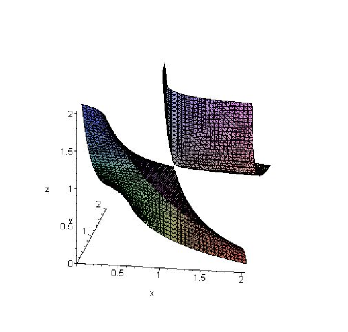
In dimension three and above, there are many further possibilities. The simplest case not handled by previous techniques is that of isolated quadratic singularity. The purpose of this paper is to address this type of generating function. All the examples Section 4 are of this type. In fact, all the rational 3-variable generating functions we know of, that are not one of the types previous analyzed, have isolated, usually quadratic, singularities. The simplest case is when the denominator is irreducible and its variety has a single, isolated quadratic singularity; a concrete example in dimension $d=3$ is the cube grove creation generating function, whose denominator $Q=1+XYZ-(X+Y+Z+XY+YZ+ZX)/3$ has the zero set illustrated in figure 1.

Refer to caption — Figure 1: an isolated quadratic singularity

The main results of this paper, Theorems 3.7 and 3.9 below, are asymptotic formulae for the coefficients of a generating function having a divisor with this geometry. In addition to one or more isolated quadratic singularities, our most general results allow $Q$ to be taken to an arbitrary real power and we allow the possibility of other smooth divisors passing through the singularities of $Q$ . These generalizations complicate the exposition somewhat but are necessary to handle some of the motivating examples.

As a preview of the behavior of the coefficients, consider the case $d=3$ and $F=1/Q$ illustrated in figure 1. The leading homogeneous term of $Q$ in the variables $(x,y,z)=(\log X,\log Y,\log Z)$ is $xy+xz+yz$ . The outward normal cone (dual cone) at this point is the cone ${\bf N^{*}}$ on which $Q^{*}\geq 0$ , where $Q^{*}(r,s,t)=(r+s+t)^{2}-2(r^{2}+s^{2}+t^{2})$ is the dual quadratic to $Q$ (see Section 2.6 for definitions). The asymptotics for $a_{\bf r}$ in this example are given by Corollary 3.8 for ${\bf r}$ in the interior of ${\bf N^{*}}$ and by an easier result (Proposition 2.23) when ${\bf r}\notin{\bf N^{*}}$ :

a_{\bf r}\sim\begin{cases}CQ^{*}({\bf r})^{-1/2}&\mbox{ if ${\bf r}$ is in the interior of }{\bf N^{*}}\\ \mbox{exponentially small }&\mbox{ if }{\bf r}\notin{\bf N^{*}}\end{cases}

The behavior of $a_{\bf r}$ near $\partial{\bf N^{*}}$ is more complicated and is not dealt with in this paper. The generating function $1/Q$ is the creation rate generating function for cube groves, discussed in Section 4.2. The edge placement generating function for cube groves (edge placement probabilities have more direct interpretations than do creation rates) has an extra factor of $(1-Z)$ in the denominator. Theorem 3.9 gives the asymptotics in this case, for ${\bf r}$ interior to ${\bf N^{*}}$ , as

a_{\bf r}\sim C\arctan\theta({\bf r})

where $\theta$ is a homogeneous degree $0$ function of ${\bf r}$ which can be expressed in terms of dual quadratic form $Q^{*}$ . Homogeneity of $\theta$ implies that that there is a limit theorem $a_{\lambda{\bf r}}\to\theta(\hat{{\bf r}})$ as $\lambda\to\infty$ , where $\hat{{\bf r}}:={\bf r}/|{\bf r}|$ is the unit vector in the direction ${\bf r}$ .

A total of five motivating applications will be discussed in detail in Section 4. All of these may be seen to have factors with isolated quadratic singularities. There are known trivariate rational generating functions with isolated singularities that are not quadratic. For example, the diabolo or fortress tiling ensemble has an isolated quartic singularity DGIP [11]. Some of our results apply to this case, but a detailed analysis will be left for another paper. The last example goes slightly beyond what we do in this paper, but we include it because the analysis follows largely the same methods.

Aztec diamond placement probability generating function JPS [98]

F(X,Y,Z)=\frac{Z/2}{(1-YZ)(1-\frac{Z}{2}(X+X^{-1}+Y+Y^{-1})+Z^{2})}\,.

(1.3)

Cube groves edge probability generating function PS [05]

F(X,Y,Z)=\frac{2Z^{2}}{3(1-Z)(1+XYZ-\frac{1}{3}(X+Y+Z+XY+XZ+YZ))}\,.\\

(1.4)

Quantum random walk space-time probability generating function ABN+ [01]; BBBP [08]

F(X,Y,Z)=\frac{XZ-(1+XY)Z^{2}+YZ^{3})}{(1-Z^{2})(1-(X+X^{-1}+Y+Y^{-1})Z/2+Z^{2})}\,.\\

(1.5)

Friedrichs-Lewy-Szegö graph polynomial SS [06]

F(X,Y,Z)=\left[(1-X)(1-Y)+(1-X)(1-Z)+(1-Y)(1-Z)\right]^{-\beta}

(1.6)

Multi-set permutation generating function Ges [92]

G(X,Y,Z)=\frac{1}{1-X-Y-Z+4XYZ}\,.

(1.7)

1.2 Methods and organization

Our methods of analysis owe a great debt to two bodies of existing theory. Our approach to harmonic analysis of cones is fashioned after the work of ABG [70]. We not only quote their results on generalized Fourier transforms, which date back somewhat farther to computations of Rie [49] and generalized function theory as described in GS [64], but we also employ their results on hyperbolic polynomials to produce homotopies of various contours. Secondly, our understanding of the existence of these homotopies has been greatly informed by Morse theoretic results of GM [88]. We do not quote these results directly because our setting does not satisfy all their hypotheses, but the idea to piece together deformations local to strata is really the central idea behind stratified Morse theory as explained in GM [88]; see also the discussion of stratified critical points in Section 2.5.

An outline our methods is as follows. The chain of integration in the multivariate Cauchy integral (1.2) is a $d$ -dimensional torus $T$ embedded in the complex torus $({\mathbb{C}}^{*})^{d}$ , where ${\mathbb{C}}^{*}:={\mathbb{C}}-\{0\}$ . Changing variables by $Z_{j}=\exp(z_{j})$ , the chain of integration becomes a chain ${\cal C}$ , the set of points with a fixed real part. Under this change of variables, the Cauchy integral (1.2) becomes

\int_{{\cal C}}\exp(-{\bf r}\cdot{\bf z})f({\bf z})\,d{\bf z}

(1.8)

where $f:=F\circ\exp$ . Letting ${\bf z}:={\bf x}+i{\bf y}$ , Morse theoretic considerations tell us we can deform the chain of integration so that it is supported by the region where $e^{-{\bf r}\cdot{\bf x}}$ is small (for large $|{\bf r}|$ ) except near certain critical points. To elaborate, we can accomplish most of the deformation by moving ${\bf x}$ . The allowable region for such deformations of ${\bf x}$ is a component of the complement to amoeba of $F$ (see Section 2.1 for definitions). Heuristically, we move ${\bf x}$ to the support point ${{\bf x}_{\min}}$ on the boundary of this region for a hyperplane orthogonal to ${\bf r}$ (see Sections 2.5 and those preceding for details). Unfortunately, when ${{\bf x}_{\min}}$ is on the boundary, (1.8) fails to be integrable. Ignoring this, however, and continuing with the heuristic, we let $q:=Q\circ\exp$ and $h_{j}:=H_{j}\circ\exp$ and we denote the leading homogeneous parts of $q$ and $h_{j}$ by ${\tilde{q}}$ and ${\tilde{h}}_{j}$ respectively. We then express $f$ near ${{\bf x}_{\min}}$ as a series in negative powers of ${\tilde{q}}$ and ${\tilde{h}}_{j}$ (this is carried out in Section 2.7). Integrating term by term, each integral has the form

\int_{\cal C}\exp(-{\bf r}\cdot{\bf z})\frac{{\bf z}^{\bf m}}{{\tilde{q}}({\bf z})^{s}{\tilde{h}}({\bf z})^{\bf n}}\,d{\bf z}

where ${\tilde{h}}^{\bf n}:=\prod_{j=1}^{k}h_{j}^{n_{j}}$ . Replacing ${\bf z}$ by $i{\bf z}$ , we recognize the Fourier transform of a product of a monomial with inverse powers of quadratics and linear functions. The Fourier transform of an inverse quadratic is the dual quadratic and the Fourier transform of a linear function is the Heaviside function. The Fourier transform of a product is a convolution. These facts tell us what result to expect.

Much of what has been described thus far is based on known methods and results, most of which are collected in the preliminary Section 2. The bulk of the work, however, is in making rigorous these identities which involve Fourier integrals that do not converge, taken over regions which are not obviously deformations of each other (the part above where we said, “ignoring this, $\ldots$ ”). For this purpose, some carefully chosen deformations are constructed, based largely on deformations found in Sections 5 and 6 of ABG [70]. Specifically, we use results on hyperbolic polynomials (see Section 2.3 for definitions) established in ABG [70] and elsewhere, to construct certain vector fields on ${\mathbb{C}}^{d}$ . These vector fields, based on the construction of [ABG, 70, Section 5] and described in our Section 5.1, then allow us to construct deformations in Section 5.2, which satisfy several properties. First, they enact what Morse theory has guaranteed: they push the chain of integration to where the integrand of (1.8) is very small, except near critical points, as in figure 2 below. Secondly, they do this without intersecting ${\cal V}$ , thereby allowing the integral to remain the same. This localizes the integral to the critical points, and allows us to concentrate on one critical point at a time. The resulting chain of integration is depicted in figure 2.

Thirdly, they allow us to “straighten out” the chain of integration. Figure 3 shows that the chains in figure 2, as well as the original chain, are homotopic near the critical point to a (slightly perturbed) conical chain.

Combined with the series expansion by homogeneous functions, this reduces all necessary integrals to a small class of Fourier-type integrals. Many of these are evaluated as generalized functions in ABG [70]; Rie [49]; GS [64] and elsewhere. In Section 6.2 and 6.3 we summarize the relevant facts about generalized functions. The above deformations allow us to show, in Sections 6.4 – 6.6, that these generalized functions, defined as integrals over the straight contour on the left of figure 3, do approximate the integrals we are interested in, which we must evaluate over the chains shown on the right of figure 2 and on figure 3 in order for the localizations to remain valid. Not all of the computations we need are available in the literature. In Section 6.6 we use a construction from ABG [70], the Leray cycle, along with a residue computation, to reduce the Fourier transform of $1/({\tilde{q}}\cdot{\tilde{h}})$ to an explicitly computable one-dimensional integral. It is this computation that is responsible for the explicit asymptotic formula for placement probabilities in the Aztec Diamond and Cube Grove problems.

To summarize, the organization of the rest of the paper is as follows. Section 2 defines some notation in use throughout the paper, and collects preliminary results on amoebas, convex duals, hyperbolicity, and expansions by powers of homogeneous polynomials. Section 3 states the main results. Section 4 has five subsections, each discussing one of the five examples. The next two sections are concerned with the proofs of the main results. Section 5 constructs homotopies that shift contours of integration, while Section 6 evaluates several classes of integrals via the theory of generalized Fourier transforms. Finally, Section 7 concludes with a discussion of open problems and further research directions.

1.3 Comparison with other techniques

One might ask, in a paper of this length, whether this is the best way to obtain these results. To answer this, we briefly review comparable published results and a relevant unpublished failure. The Arctic Circle Theorem for tilings of the Aztec diamond was proved in CEP [96] in two steps. First formulae for the coefficients of the simpler creation rate generating function $(1-(X+X^{-1}+Y+Y^{-1})Z/2+Z^{2})^{-1}$ were derived via a relation to Krawtchouk polynomials. Secondly, these were summed by means of contour integrals. The computation was quite specialized, and did not generalize even to the nearly formally equivalent case of cube groves. In fact, for the cube grove model, up to now only the easy half of the Arctic Circle theorem was proved (exponential decay outside of the circle).

The present paper takes the view that the work is justifiable if we can then crank out results with relatively little effort. The continuous setting clarifies matters considerably. Our fundamental result, Theorem 3.7 below, is that the asymptotics of a generating functions with irreducible quadratic denominator, such as in (1.6), are its Fourier transform, which is the dual quadratic. This is the continuous analogue of the Krawtchouk polynomials that appear when the computations are done in the discrete setting. Multiplying the denominator by $1/h$ where $h$ is smooth, corresponds to convolving the Fourier transform with a heavyside function; this is the analogue of summing and is made rigorous in Theorem 3.9. These two facts (Fourier transform of a cone is the dual cone, and Fourier transform of $1/(Qh)$ is the integral of the Fourier transform of $1/Q$ ) are well known, which makes the resulting computation predictable although a number of details need to be addressed.

As far as we know, the Aztec diamond result is the only one of the five results in Section 4 that was previously known; all five examples are easily handled once the machine is built. A sixth example, the fortress tiling ensemble, can be analyzed by our methods but explicit formulae in this case require further computations along the lines of Section 6.6. The limit theorem is known in this case, the result of a variational equation which is established and explicitly solved in the beautiful paper KO [07].

It should be emphasized that evaluating the integral (1.8) involves interplay between the form and the chain, and this interplay which is primarily responsible for failure of several earlier attempts to analyse the asymptotics of the integral. To be sure, resolution of singularities provides one with an efficient toolbox for reducing the integrand to a monomial form; see for instance [AGZV, 88, Chapter 7] or Jea [70]; the resolution is in principle effective BM [97] and the algorithm given in Var [77] suffices in most cases. However, it then becomes difficult to control the chain of integration. A few years ago, the second author in collaboration with H. Cohn attempted to resolve the singularity and compute the integral. The resolution was indeed computable. Unfortunately, as will be true in all such cases, the phase function becomes quite degenerate, being constant along the exceptional divisor of the resolution. The resulting integral was beyond Cohn and Pemantle’s ability to evaluate.

Another important aspect of the problem that is difficult to control using resolution of singularities is the real structure. Consequences of this include hyperbolicity of the tangent cones to the pole variety at critical points (see Section 2.4). As we will see, this hyperbolicity plays a critical role in the constructions of the deformations of the integration chains.

2 Notation and preliminaries

Several notions arising repeatedly in this paper are the logarithmic change of variables, duality between ${\bf r}$ and ${\bf z}$ , and the leading homogeneous part of a function. We employ some meta-notation designed for ease of keeping track of these. We use upper case letters for variables and functions in the complex torus $({\mathbb{C}}^{*})^{d}$ , and lower case letters in the logarithmic coordinates. We will never use the notations without defining them, but knowing that, for example, $F\circ\exp$ will always be denoted $f$ and ${\bf z}$ will always be $\log{\bf Z}$ , should help the reader quickly recognize the setting. We will always use ${\bf x}$ and ${\bf y}$ for the real and imaginary parts of the vector ${\bf z}\in{\mathbb{C}}^{d}$ . Boldface is reserved for vectors. The leading homogeneous part of a function is denoted with a bar. Rather than considering the index ${\bf r}$ of $a_{\bf r}$ to be an element of ${\mathbb{Z}}^{d}$ , we consider it to be an element of a space $({\mathbb{R}}^{d})^{*}$ that is dual to the domain ${\mathbb{C}}^{d}$ in which ${\bf z}$ lives, with respect to the pairing ${\bf r}\cdot{\bf z}$ (the space $({\mathbb{R}}^{d})^{*}$ is a subset of the full dual space $({\mathbb{C}}^{d})^{*}$ but all our dual vectors will be real). Many functions of ${\bf r}$ use in what follows are homogeneous degree $0$ ; letting $\hat{{\bf r}}$ denote the unit vector ${\bf r}/|{\bf r}|$ we will often write these as functions of $\hat{{\bf r}}$ . The logarithm and exponential functions are extended to act coordinatewise on vectors. Thus

	$\displaystyle\exp(z_{1},\ldots,z_{d})$	$\displaystyle:=$	$\displaystyle(\exp(z_{1}),\ldots,\exp(z_{d}))\,;$
	$\displaystyle\log(Z_{1},\ldots,Z_{d})$	$\displaystyle:=$	$\displaystyle(\log(Z_{1}),\ldots,\log(Z_{d}))\,.$

We also employ the slightly clunky notation

{\rm ReLog\,}{\bf Z}\,:=\,(\log|Z_{1}|,\ldots,\log|Z_{d}|)\,=\,{\rm Re\,}\{\log{\bf Z}\}

for the coordinatewise log-modulus map, having found that the notations in use in GKZ [94] do not allow for quick visual distinction between $\log$ and ${\rm ReLog\,}$ .

Our chief concern is with generating functions that are ordinary power series, convergent on the unit polydisk, and whose denominator is the product of smooth and quadratically singular factors that intersect the closed but not the open unit polydisk. It costs little, however, and there is some benefit to work in the greater generality of Laurent series representing functions with polynomial denominators. Indeed, Laurent series arise naturally in the examples (though these Laurent series have exponents in proper cones, and may therefore be reduced by log-affine changes of coordinates to Taylor series).

Definition 2.1 (homogeneous part).

For analytic germ $f:({\mathbb{C}}^{d},{\bf z})\to{\mathbb{C}}$ at a point ${\bf z}\in{\mathbb{C}}^{d}$ , we let $\deg(f,{\bf z})$ denote the degree of vanishing of $f$ at ${\bf z}$ . This is zero if $f({\bf z})\neq 0$ and in general is the greatest integer $n$ such that $f({\bf z}+{\bf w})=O(|{\bf w}|^{n})$ as ${\bf w}\to{\bf 0}$ . Also, $\deg(f,{\bf z})$ is the least degree of any monomial in the ordinary power series expansion of $f({\bf z}+\cdot)$ around ${\bf 0}$ . We let $\mbox{\elevenss hom}(f,{\bf z})$ denote the sum of all monomials of minimal degree in the power series for $f({\bf z}+\cdot)$ and we call this the homogeneous part of $f$ at ${\bf z}$ . Thus

f({\bf z}+{\bf w})=\mbox{\elevenss hom}(f,{\bf z})({\bf w})+O\left(|{\bf w}|^{\deg(f,{\bf z})+1}\right)\,

for small $|{\bf w}|$ .When ${\bf z}={\bf 0}$ , we may omit ${\bf z}$ from the notation: thus, $\mbox{\elevenss hom}(f):=\mbox{\elevenss hom}(f,{\bf 0})$ .

A number of connections between zeros of a Laurent polynomial $F$ , the Laurent series for $1/F$ , the Newton polytope for $F$ and certain dual cones to this polygon were worked out in the 1990’s by Gelfand, Kapranov and Zelivinsky. We summarize some relevant results from [GKZ, 94, Chapter 6].

2.1 The Log map and amoebas

Let $F$ be a Laurent polynomial in $d$ variables. Let $({\mathbb{C}}^{*})^{d}\subseteq{\mathbb{C}}^{d}$ denote the $d$ -tuples of nonvanishing complex numbers and let ${\cal V}_{F}$ denote the zero set of $F$ in $({\mathbb{C}}^{*})^{d}$ . Following GKZ [94] we define the amoeba of $F$ to be the image under ${\rm ReLog\,}$ of the zero set of $F$ :

{\mbox{\elevenss amoeba}}(F):=\{{\rm ReLog\,}{\bf z}:{\bf z}\in{\cal V}_{F}\cap({\mathbb{C}}^{*})^{d}\}\subseteq{\mathbb{R}}^{d}\,.

The simplest example is the amoeba of a linear function, such as $F=2-X-Y$ , shown in figure 4(a). The amoeba of a product is the union of amoebas, as shown in figure 4(b).

The rational function $1/F$ has, in general, a number of Laurent series expansions, each convergent on a different subset of ${\mathbb{C}}^{d}$ . Combining Corollary 1.6 in Chapter 6 of GKZ [94] with Cauchy’s integral theorem, we have the following result.

Proposition 2.2.

The connected components of ${\mathbb{R}}^{d}\setminus{\mbox{\elevenss amoeba}}(F)$ are convex open sets. The components are in bijective correspondence with Laurent series expansions for $1/F$ as follows. Given a Laurent series expansion of $1/F$ , its open domain of convergence is precisely ${\rm ReLog\,}^{-1}B$ where $B$ is a component of ${\mathbb{R}}^{d}\setminus{\mbox{\elevenss amoeba}}(F)$ . Conversely, given such a component $B$ , a Laurent series $1/F=\sum a_{\bf r}{\bf Z}^{\bf r}$ convergent on $B$ may be computed by the formula

a_{\bf r}=\frac{1}{(2\pi i)^{d}}\int_{\bf T}{\bf Z}^{-{\bf r}-{\bf 1}}\frac{1}{F({\bf Z})}\,d{\bf Z}

where ${\bf T}$ is the torus ${\rm ReLog\,}^{-1}({\bf x})$ for any ${\bf x}\in B$ . Changing variables to ${\bf Z}=\exp({\bf z})$ and $d{\bf Z}={\bf Z}\,d{\bf z}$ gives

a_{\bf r}=\frac{1}{(2\pi i)^{d}}\int_{{\bf x}+iT_{\mathbb{R}}}e^{-{\bf r}\cdot{\bf z}}\frac{1}{f({\bf z})}\,d{\bf z}

(2.1)

where $f=F\circ\exp$ and $T_{\mathbb{R}}$ is the torus $R^{d}/(2\pi{\mathbb{Z}})^{d}$ . $\hfill\Box$

2.2 Dual cones, tangent cones and normal cones

Let $({\mathbb{R}}^{d})^{*}$ denote the dual space to ${\mathbb{R}}^{d}$ and for ${\bf y}\in{\mathbb{R}}^{d}$ and ${\bf r}\in({\mathbb{R}}^{d})^{*}$ , use the notation ${\bf r}\cdot{\bf y}$ to denote the pairing. Let ${\bf L}$ be any convex open cone in ${\mathbb{R}}^{d}$ . The (closed) convex dual cone ${\bf L^{*}}\subseteq({\mathbb{R}}^{d})^{*}$ is defined to be the set of vectors ${\bf v}\in({\mathbb{R}}^{d})^{*}$ such that ${\bf v}\cdot{\bf x}\geq 0$ for all ${\bf x}\in{\bf L}$ . Familiar properties of the dual cone are

	$\displaystyle L\subseteq M$	$\displaystyle\Rightarrow$	$\displaystyle L^{}\supseteq M^{}\,;$		(2.2)
	$\displaystyle(L\cap M)^{*}$	$\displaystyle=$	$\displaystyle\mbox{\elevenss hull}\,(L^{}\cup M^{})\,.$		(2.3)

Suppose ${\bf x}$ is a point on the boundary of a convex set $C$ . Then the intersection of all halfspaces that contain $C$ and have ${\bf x}$ on their boundary is a closed convex affine cone with vertex ${\bf x}$ (a translation by ${\bf x}$ of a closed convex cone in ${\mathbb{R}}^{d}$ ) that contains $C$ . Translating by $-{\bf x}$ and taking the interior gives the (open) tangent cone to $C$ at ${\bf x}$ , denoted by $\mbox{\elevenss tan}_{\bf x}(C)$ . An alternative definition is

\mbox{\elevenss tan}_{\bf x}(C)=\{{\bf v}:{\bf x}+\epsilon{\bf v}\in C\mbox{ for all sufficiently small }\epsilon>0\}\,

(where $B$ is the unit ball). The (closed) normal cone to $C$ at ${\bf x}$ , denoted ${\bf N}_{\bf x}^{*}(C)$ , is the convex dual cone to the negative of the tangent cone:

{\bf N}_{\bf x}^{*}(C)=(-\mbox{\elevenss tan}_{\bf x}(C))^{*}\,.

Equivalently, it corresponds to the set of linear functionals on $C$ that are maximized at ${\bf x}$ , or to the set of outward normals to support hyperplanes to $C$ at ${\bf x}$ .

Definition 2.3 (proper dual direction).

Given a convex set $C$ , say that ${\bf r}$ is a proper direction for $C$ if the maximum of ${\bf r}\cdot{\bf x}$ on $L$ is achieved at a unique ${{\bf x}_{\min}}\in\overline{C}$ . We call ${{\bf x}_{\min}}$ the dual point for ${\bf r}$ . The set of directions ${\bf r}$ for which ${\bf r}\cdot{\bf x}$ is bounded on $C$ but ${\bf r}$ is not proper has measure zero.

The term tangent cone has a different meaning in algebraic contexts, which we will require as well. (The term normal cone has an algebraic meaning as well, which we will not need.) To avoid confusion, we define the algebraic tangent cone of $f$ at ${\bf x}$ to be ${\cal V}_{\mbox{\elevenss hom}(f,{\bf z})}$ . An equivalent but more geometric definition is that the algebraic tangent cone is the union of lines through ${\bf x}$ that are the limits of secant lines through ${\bf x}$ ; thus for a unit vector ${\bf u}$ , the line ${\bf x}+t{\bf u}$ is in the algebraic tangent cone if there are ${\bf x}_{n}\in{\cal V}_{f}$ distinct from but converging to ${\bf x}$ for which $({\bf x}_{n}-{\bf x})/||{\bf x}_{n}-{\bf x}||\to\pm{\bf u}$ . This equivalence and more is contained in the following results. We let $S_{1}$ denote the unit sphere $\{(z_{1},\ldots,z_{d}):|z_{1}|^{2}+\cdots+|z_{d}|^{2}=1\}$ and let $S_{r}:=rS_{1}$ denote the sphere of radius $r$ .

Lemma 2.4 (algebraic tangent cone is the limiting secant cone).

Let $q$ be a polynomial vanishing to degree $m\geq 1$ at the origin and let ${\tilde{q}}:=\mbox{\elevenss hom}(q)$ be its homogeneous part; in particular,

q({\bf z})={\tilde{q}}({\bf z})+R({\bf z})

where ${\tilde{q}}$ is a nonzero homogeneous polynomial of degree $m$ and $R({\bf z})=O(|{\bf z}|^{m+1})$ . Let $q_{\epsilon}$ denote the polynomial

q_{\epsilon}({\bf z}):=\epsilon^{-m}q(\epsilon{\bf z})={\tilde{q}}({\bf z})+R_{\epsilon}({\bf z})

where $R_{\epsilon}({\bf z})=\epsilon^{-m}R(\epsilon{\bf z})\to 0$ as $\epsilon\to 0$ . Let ${\cal V}_{\epsilon}:={\cal V}_{q_{\epsilon}}\cap S_{1}$ denote the intersection of $\{q_{\epsilon}=0\}$ with the unit sphere. Then ${\cal V}_{\epsilon}$ converges in the Hausdorff metric as $\epsilon\to 0$ to ${\cal V}_{{\tilde{q}}}\cap S_{1}$ .

Proof: On any compact set, in particular $S_{1}$ , $R_{\epsilon}\to 0$ uniformly. If ${\bf z}^{(n)}\to{\bf z}$ and ${\bf z}^{(n)}\in{\cal V}_{1/n}$ then for each $n$ ,

|{\tilde{q}}({\bf z}^{(n)})|=|q_{1/n}({\bf z}^{(n)})+R_{1/n}({\bf z}^{(n)})|=|R_{1/n}({\bf z}^{(n)})|\to 0\,.

Hence ${\tilde{q}}({\bf z})=0$ by continuity of ${\tilde{q}}$ and we see that any limit point of ${\cal V}_{\epsilon}$ as $\epsilon\to 0$ is in ${\cal V}_{{\tilde{q}}}\cap S_{1}$ . Conversely, fix a unit vector ${\bf z}\in{\cal V}_{{\tilde{q}}}$ . The homogenous polynomial ${\tilde{q}}$ is not identically zero, therefore there is a projective line through $\overline{{\bf z}}$ along which ${\tilde{q}}$ has a zero of finite order at $\overline{{\bf z}}$ . Back in affine space, there is a complex curve $\gamma$ in the unit sphere along which ${\tilde{q}}$ is holomorphic with a zero of some finite order $k$ at ${\bf z}$ . As $\epsilon\to 0$ , the holomorphic function $R_{\epsilon}$ goes to zero uniformly in a neighborhood of ${\bf z}$ in $\gamma$ ; hence there are $k$ zeros of $q_{\epsilon}$ converging to ${\bf z}$ as $\epsilon\to 0$ , and therefore ${\bf z}$ is a limit point of ${\cal V}_{\epsilon}$ as $\epsilon\to 0$ . $\hfill\Box$

2.3 Hyperbolicity for homogeneous polynomials

The notion of hyperbolic polynomials arose first in Går [50] in connection with solutions to wave-like partial differential equations. The same property turns out to be very important as well for convex programming, cf. Gül [97] from which much of the next several paragraphs is drawn.

Let $f$ be a complex polynomial in $d$ -variables and $f(D)$ denote the corresponding linear partial differential operator with constant coefficients, obtained by replacing each $x_{j}$ by $\partial/\partial x_{j}$ . For example, if $f$ is the standard Lorentzian quadratic $S({\bf x}):=x_{1}^{2}-\sum_{j=2}^{d}x_{j}^{2}$ then $S(D)$ is the wave operator $(\partial/\partial x_{1})^{2}-\sum_{j=2}^{d}(\partial/\partial x_{j})^{2}$ . Gårding’s object was to determine when the equation

f(D)u=g

(2.4)

with $g$ supported on a halfspace has a solution supported in the same halfspace. The wave operator has this property, and in fact there is a unique such solution for any such $g$ . It turns out that the class of $f$ such that (2.4) always has a solution supported on the halfspace is precisely characterized by the property of being hyperbolic, as defined by Gårding. In this case, it was later shown ([Hör, 90, Theorem 12.4.2] that the solution is in fact unique. The theory of hyperbolic polynomials serves in the present paper to prove the existence of deformations of chains of integration past points of the pole manifold at which the pole polynomial is locally hyperbolic.

We begin with hyperbolicity for homogeneous polynomials, which is a simpler and better developed theory. We use $A$ rather than $f$ for a homogeneous polynomial.

Definition 2.5 (hyperbolicity).

Say that a homogeneous complex polynomial $A$ of degree $m\geq 1$ is hyperbolic in direction ${\bf v}\in{\mathbb{R}}^{d}$ if $A({\bf v})\neq 0$ and the polynomial $A({\bf x}+t{\bf v})$ has only real roots when ${\bf x}$ is real. In other words, every line in real space parallel to ${\bf v}$ intersects ${\cal V}_{A}$ exactly $m$ times (counting multiplicities).

While seemingly weaker, the requirement of avoiding purely imaginary roots is in fact easily seen to be equivalent.

Proposition 2.6.

Hyperbolicity of the homogeneous polynomial $A$ in the direction ${\bf v}$ is equivalent to the condition that $A({\bf v}+i{\bf y})\neq 0$ for all ${\bf y}\in{\mathbb{R}}^{d}$ .

Proof: Because $A$ is homogeneous, when $\lambda\neq 0$ , we have $A(\lambda{\bf z})=0$ if and only if $A({\bf z})=0$ . With $\lambda=i\cdot s$ , a purely imaginary number not equal to zero, we see that $A({\bf v}+i{\bf y})\neq 0$ for all ${\bf y}\in{\mathbb{R}}^{d}$ is equivalent to $A({\bf y}+is{\bf v})\neq 0$ for all ${\bf y}\in{\mathbb{R}}^{d}$ and all nonzero real $s$ . This becomes $A({\bf y}+t{\bf u}+is{\bf u})\neq 0$ for all ${\bf y}\in{\mathbb{R}}^{d}$ and real $s\neq 0$ ; writing $z=t+is$ , this is equivalent to $A({\bf y}+z{\bf u})\neq 0$ when $z$ is not real, which is the definition of hyperbolicity. $\hfill\Box$

The further properties we need are well known and are proved, among other places, in [Gül, 97, Theorem 3.1].

Proposition 2.7.

The set of ${\bf v}$ for which $A$ is hyperbolic in direction ${\bf v}$ is an open set whose components are convex cones. Denote by ${\bf K}^{\bf v}(A)$ the connected component of this cone that contains a given ${\bf v}$ . Some multiple of $A$ is positive on ${\bf K}^{\bf v}(A)$ and vanishing on $\partial{\bf K}^{\bf v}(A)$ , and for ${\bf x}\in{\bf K}^{\bf v}(A)$ , the roots of $A({\bf x}+t{\bf v})$ will all be negative. $\hfill\Box$

Semi-continuity properties for cones of hyperbolicity play a large role in the construction of deformations. A lower semi-continuous function $f$ satisfies $f(x)\leq\liminf_{y\to x}f(y)$ . The property is important in elementary analysis because a lower semi-continuous function on a compact set achieves its infimum; generalizing to set-valued functions, the conclusion is roughly that the empty set is not a limit value and therefore that a continuous section can be defined. In this section, we develop semi-continuity properties for cones of hyperbolicity (a topic that occupies many pages of ABG [70]).

The following proposition and definition define a family of cones $\displaystyle{\{{\bf K}^{A,B}({\bf x})\}_{{\bf x}\in{\mathbb{R}}^{d}}}$ which will be used to prove two critical semi-continuity results for cones of hyperbolicity for log-Laurent polynomials (Theorem 2.14 below).

Proposition 2.8 (first semi-continuity result).

Let $A$ be any hyperbolic homogeneous polynomial, and let $m$ be its degree. Fix ${\bf x}$ with $A({\bf x})=0$ and let $\tilde{A}:=\mbox{\elevenss hom}(A,{\bf x})$ denote the leading homogeneous part of $A$ at ${\bf x}$ . If $A$ is hyperbolic in direction ${\bf u}$ then $\tilde{A}$ is also hyperbolic in direction ${\bf u}$ . Consequently, if $B$ is any cone of hyperbolicity for $A$ then there is some cone of hyperbolicity for $\tilde{A}$ containing $B$ .

Proof: This follows from the conclusion (3.45) of [ABG, 70, Lemma 3.42]. Because the development there is long and complicated, we give here a short, self-contained proof, provided by J. Borcea (personal communication). If $P$ is a polynomial whose degree at zero is $k$ , we may recover its leading homogeneous part $\mbox{\elevenss hom}(P)$ by

\mbox{\elevenss hom}(P)({\bf y})=\lim_{\lambda\to\infty}\lambda^{k}P(\lambda^{-1}{\bf y})\,.

The limit is uniform as ${\bf y}$ varies over compact sets. Indeed, monomials of degree $k$ are invariant under the scaling on the right-hand side, while monomials of degree $k+j$ scale by $\lambda^{-j}$ , uniformly over compact sets.

Apply this with $P(\cdot)=A({\bf x}+\cdot)$ and ${\bf y}+t{\bf u}$ in place of ${\bf y}$ to see that for fixed ${\bf x},{\bf y}$ and ${\bf u}$ ,

\tilde{A}({\bf y}+t{\bf u})=\lim_{\lambda\to\infty}\lambda^{k}A({\bf x}+\lambda^{-1}({\bf y}+t{\bf u}))

uniformly as $t$ varies over compact sub-intervals of ${\mathbb{R}}$ . Because $A$ is hyperbolic in direction ${\bf u}$ , for any fixed $\lambda$ , all the zeros of this polynomial in $t$ are real. Hurwitz’ theorem on the continuity of zeros [Con, 78, Corollary 2.6] says that a limit, uniformly on bounded intervals, of polynomials having all real zeros will either have all real zeros or vanish identically. The limit $\tilde{A}({\bf y}+t{\bf u})$ has degree $k\geq 1$ ; it does not vanish identically and therefore it has all real zeros. This shows $\tilde{A}$ to be hyperbolic in direction ${\bf u}$ . $\hfill\Box$

Definition 2.9 (family of cones in the homogeneous case).

Let $A$ be a hyperbolic homogeneous polynomial and let $B$ be a cone of hyperbolicity for $A$ . If $A({\bf x})=0$ , define

{\bf K}^{A,B}({\bf x})

to be the cone of hyperbolicity of $\mbox{\elevenss hom}(A,{\bf x})$ containing $B$ , whose existence we have just proved. If $A({\bf x})\neq 0$ we define ${\bf K}^{A,B}({\bf x})$ to be all of ${\mathbb{R}}^{d}$ .

As an example of a hyperbolic polynomial, let $S=x_{1}^{2}-x_{2}^{2}-\cdots-x_{d}^{2}$ be the standard Lorentzian quadratic. Then ${\bf K}^{e_{1}}(S)$ is the Lorentz cone $\{{\bf x}:x_{1}\geq\sqrt{x_{2}^{2}+\cdots+x_{d}^{2}}\}$ . Any quadratic of Lorentizan signature is obtained from this one by a real linear transformation; we see therefore that for any Lorentzian quadratic, the boundary of the cone of hyperbolicity is the algebraic tangent cone.

The class of hyperbolic polynomials in a given direction direction ${\bf v}$ is closed under products, and ${\bf K}^{\bf v}(AA^{\prime})={\bf K}^{\bf v}(A)\cap{\bf K}^{\bf v}(A^{\prime})$ . The class contains all linear polynomials not annihilating ${\bf v}$ and all real quadratic polynomials $p$ of Lorentzian signature for which $p({\bf v})>0$ ( ${\bf v}$ is time-like).

2.4 Hyperbolicity and semi-continuity for log-Laurent polynomials on the amoeba boundary

For a function that is not locally homogeneous, there are two natural generalizations of the definition of hyperbolicity. Both are equivalent to the notion of hyperbolicity already defined, in the case of a homogeneous polynomial. Useful features of the two definitions are revealed in the subsequent two propositions.

Definition 2.10.

Let $f:{\mathbb{C}}^{d}\to{\mathbb{C}}$ vanish at ${\bf z}$ and be holomorphic in a neighborhood of ${\bf z}$ . We say that $f$ is strongly hyperbolic at ${\bf z}$ in direction of the unit vector ${\hat{\bf v}}$ if there is an $\epsilon>0$ such that $f({\bf z}+t{\bf v}^{\prime}+i{\bf u})\neq 0$ for all real $t\in(0,\epsilon)$ , all ${\bf v}^{\prime}$ with $|{\bf v}^{\prime}-{\hat{\bf v}}|<\epsilon$ , and all ${\bf u}\in{\mathbb{R}}^{d}$ of magnitude at most $\epsilon$ . In this case we may say that $f$ is strongly hyperbolic at ${\bf z}$ in direction ${\hat{\bf v}}$ with radius $\epsilon$ . Say that $f$ is weakly hyperbolic in direction ${\bf v}$ if for every $M>0$ , there is an $\epsilon>0$ such that $f({\bf z}+t{\bf v}+i{\bf u})\neq 0$ for all real $0<t|{\bf v}|<\epsilon$ , and for all ${\bf u}\in{\mathbb{R}}^{d}$ of magnitude at most $\epsilon$ additionally satisfying $|{\bf u}|/(t|{\bf v}|)\leq M$ .

Proposition 2.11.

Let $A=\mbox{\elevenss hom}(f,{\bf z})$ . Then $A$ is hyperbolic in direction ${\bf u}$ if and only if $f$ is weakly hyperbolic in direction ${\bf u}$ at ${\bf z}$ .

Proof: The homogeneous polynomial $A$ fails to be hyperbolic at in direction ${\bf u}$ if and only if there is some real ${\bf y}$ such that $A({\bf u}+i{\bf y})=0$ . By Lemma 2.4, this happens if and only if $f({\bf z}+{\bf w}_{n})=0$ for some sequence $\{{\bf w}_{n}\}$ converging to ${\bf 0}$ with ${\bf w}_{n}/|{\bf w}_{n}|$ converging to $({\bf u}+i{\bf y})/|{\bf u}+i{\bf y}|$ . This is equivalent to failure of weak hyperbolicity of $f$ at ${\bf z}$ in direction ${\bf u}$ . $\hfill\Box$

Remark.

It is immediate from the definition that strong hyperbolicity is a neighborhood property: if $f$ is strongly hyperbolic at ${\bf x}+i{\bf y}$ in direction ${\hat{\bf v}}$ with radius $\epsilon$ , then for $|{\bf y}^{\prime}-{\bf y}|<\epsilon$ and $|{\hat{\bf v}}^{\prime}-{\hat{\bf v}}|<\epsilon$ , $f$ is strongly hyperbolic at ${\bf x}+i{\bf y}^{\prime}$ in direction ${\hat{\bf v}}^{\prime}$ with direction $\epsilon-\max\{|{\bf y}^{\prime}-{\bf y}|,|{\bf v}^{\prime}-{\hat{\bf v}}|\}$ . Weak hyperbolicity of $f$ at ${\bf z}$ in direction ${\bf v}$ extends to a neighborhood of ${\bf v}$ by Propositions 2.7 and 2.11. Extending weak hyperbolicity to neighboring ${\bf z}$ is much trickier.

Proposition 2.12.

Let $F$ be a Laurent polynomial in $d$ variables. Suppose that $B$ is a component of ${\mbox{\elevenss amoeba}}(F)$ and ${\bf x}\in\partial B$ , so that $f:=F\circ\exp$ vanishes at some point ${\bf x}+i{\bf y}$ . Let ${\overline{f}}:=\mbox{\elevenss hom}(f,{\bf x}+i{\bf y})$ denote the leading homogeneous part of $f({\bf x}+i{\bf y}+\cdot)$ . Then $f$ is strongly hyperbolic at ${\bf x}+i{\bf y}$ , some complex scalar multiple of ${\overline{f}}$ is real and hyperbolic, and some cone of hyperbolicity ${\bf K}^{\bf u}({\overline{f}})$ contains $\mbox{\elevenss tan}_{\bf x}(B)$ .

Proof: Strong hyperbolicity of $f$ in any direction ${\bf u}\in\mbox{\elevenss tan}_{\bf x}(B)$ follows from the definition of the amoeba. Strong hyperbolicity is stronger than weak hyperbolicity, hence hyperbolicity of ${\overline{f}}$ in direction ${\bf u}$ follows from Proposition 2.11. The vector ${\bf u}\in\mbox{\elevenss tan}_{\bf x}(B)$ is arbitrary, whence ${\bf K}^{\bf u}({\overline{f}})\supseteq\mbox{\elevenss tan}_{\bf x}(B)$ . To see that some multiple of ${\overline{f}}$ is real, let ${\bf u}$ be any real vector in $\mbox{\elevenss tan}_{\bf x}(B)$ , let $m$ denote the degree of ${\overline{f}}$ , and let $\gamma$ denote the coefficient of the $z^{m}$ term of $A({\overline{f}}{\bf u}+{\bf y})$ . Then $\gamma$ is the degree $m$ coefficient of ${\overline{f}}(z{\bf u})$ , hence is nonzero and does not depend on ${\bf y}$ . For any fixed ${\bf y}$ , the fact that ${\overline{f}}(z{\bf u}+{\bf y})$ has all real roots implies that the monic polynomial $\gamma^{-1}{\overline{f}}(z{\bf u}+{\bf y})$ has all real coefficients. $\hfill\Box$

Definition 2.13 (hyperbolicity and normal cones at a point of ${\cal V}_{f}$ ).

Let $F$ be a Laurent polynomial, $B$ a component of ${\mathbb{R}}^{d}\setminus{\mbox{\elevenss amoeba}}(F)$ , and ${\bf Z}=\exp({\bf x}+i{\bf y})\in{\cal V}_{f}$ with ${\bf x}\in\partial B$ . We let $f:=F\circ\exp$ and let

{\bf K}^{f,B}({\bf Z}):={\bf K}^{\bf u}(\mbox{\elevenss hom}(f,{\bf x}+i{\bf y}))\,,

(2.5)

denote the (open) cone of hyperbolicity of ${\overline{f}}:=\mbox{\elevenss hom}(f,{\bf x}+i{\bf y})$ that contains $B$ , whose existence is guaranteed by Proposition 2.12. Although it is a slight abuse of notation, we also write

{\bf K}^{f,B}({\bf y}):={\bf K}^{f,B}({\bf Z})

when ${\bf Z}=\exp({\bf x}+i{\bf y})$ and the specification of ${\bf x}$ is clearly understood. We also define the normal cone

{\bf N^{*}}({\bf Z}):=({\bf N^{*}})^{f,B}({\bf Z})=({\bf K}^{f,B}({\bf Z}))^{*}\,.

(2.6)

We see immediately from Proposition 2.12 that

{\bf K}^{f,B}({\bf Z})\supseteq\tan_{\bf x}(B)

(2.7)

and hence

{\bf N^{*}}({\bf Z})\subseteq{\bf N}_{\bf x}^{*}(B)\,.

In order to produce deformations, we will need to know that the cones ${\bf K}^{f,B}({\bf Z})$ vary semi-continuously as ${\bf Z}$ varies over the torus $\exp({\bf x}+i{\mathbb{R}}^{d})$ . We have seen already that all of these cones contain $\mbox{\elevenss tan}_{\bf x}(B)$ . What is needed, therefore, is an argument showing that ${\bf K}^{f,B}({\bf Z}^{\prime})$ contains any ${\bf u}\in{\bf K}^{f,B}({\bf Z})$ when ${\bf Z}^{\prime}$ is sufficiently close to ${\bf Z}$ and ${\bf u}\notin\mbox{\elevenss tan}_{\bf x}(B)$ . In fact, not every polynomial admits a semi-continuous choice of tangent subcone; a counterexample is $xy+z^{3}$ . However, in the case where ${\bf x}\in\partial B$ , we are able to use strong hyperbolicity in directions ${\bf v}\in\mbox{\elevenss tan}_{\bf x}(B)$ to prove semi-continuity even outside of $\mbox{\elevenss tan}_{\bf x}(B)$ . The main result of this section is exactly such an analogue of Proposition 2.8:

Theorem 2.14.

Suppose that an analytic function $f$ is strongly hyperbolic in direction ${\bf v}$ at the point ${\bf z}={\bf x}+i{\bf y}$ . Let ${\overline{f}}:=\mbox{\elevenss hom}({\overline{f}},{\bf z})$ . Let ${\bf u}\in{\bf K}^{\bf v}({\overline{f}})$ be any point in the cone of hyperbolicity of ${\overline{f}}$ containing ${\bf v}$ . Then $f$ is strongly hyperbolic in direction $\alpha{\bf v}+(1-\alpha){\bf u}$ for every $0\leq\alpha\leq 1$ .

Corollary 2.15.

$(i)$ If $B$ is a component of ${\mbox{\elevenss amoeba}}(F)^{c}$ and ${\bf x}\in\partial B$ , then ${\bf K}^{f,B}({\bf Z})$ is semi-continuous in ${\bf Z}$ as ${\bf y}$ varies with ${\bf Z}=\exp({\bf x}+i{\bf y})$ , meaning that ${\bf K}^{f,B}({\bf Z})\subseteq\liminf_{{\bf Z}^{\prime}}{\bf K}^{f,B}({\bf Z}^{\prime})$ .

$(ii)$ If $A$ is a homogeneous polynomial and $B$ is a cone of hyperbolicity for $A$ , then ${\bf K}^{A,B}({\bf y})$ is semi-continuous in ${\bf y}$ .

Proof: Pick any ${\bf v}\in\mbox{\elevenss tan}_{\bf x}(B)$ . The function $f$ is strongly hyperbolic in direction ${\bf v}$ , hence by Theorem 2.14, it is strongly hyperbolic at ${\bf x}+i{\bf y}$ in every direction ${\bf u}\in{\bf K}^{\bf v}({\overline{f}})$ . Because strong hyperbolicity is a neighborhood property, it follows that for every ${\bf y}^{\prime}$ in some neighborhood of ${\bf y}$ , some cone of hyperbolicity of ${\overline{f}}$ contains ${\bf K}^{\bf v}(f)$ . All these cones contain ${\bf v}$ , hence these are the cones ${\bf K}^{f,B}({\bf Z}^{\prime})$ (with ${\bf Z}^{\prime}:=\exp({\bf x}+i{\bf y}^{\prime})$ ), and hence all these cones contain ${\bf K}^{f,B}({\bf Z})$ . The proof in the homogeneous case is analogous, again because each $\tilde{A}:=\mbox{\elevenss hom}(A,{\bf y})$ is strongly hyperbolic in direction ${\bf v}$ for any ${\bf v}\in B$ . $\hfill\Box$

Proof of Theorem 2.14: The proof is based on a technique of Gårding [Går, 50, Theorem H 5.4.4] that is used in the proof of [ABG, 70, Lemma 3.22]. Let $f$ be strongly hyperbolic at ${\bf x}+i{\bf y}$ in direction ${\bf v}$ with radius $\epsilon$ and choose any ${\bf u}\in{\bf K}^{\bf v}(f)$ . For the remainder of this argument, we assume that ${\bf y}^{\prime}$ and ${\hat{\bf v}}^{\prime}$ satisfy

|{\bf y}^{\prime}-{\bf y}|,|{\hat{\bf v}}^{\prime}-{\hat{\bf v}}|<\frac{\epsilon}{2}\,;

a consequence is that $f$ is strongly hyperbolic in direction ${\hat{\bf v}}^{\prime}$ at ${\bf x}+i{\bf y}^{\prime}$ with radius $\epsilon/2$ . For any ${\bf b}\in{\mathbb{R}}^{d}$ , if $s$ is purely imaginary with $|s||{\bf b}|<\epsilon/2$ , then the imaginary vector $s{\bf b}+i({\bf y}^{\prime}-{\bf y})$ will have magnitude less than $\epsilon$ . By hypothesis, when $0<t<\epsilon$ , the function

s\mapsto f({\bf x}+i{\bf y}^{\prime}+s{\bf b}+t{\hat{\bf v}}^{\prime})

(2.8)

will therefore be nonzero.

As the complex argument $s$ tends to zero, there is an expansion

f({\bf x}+i{\bf y}+s(\alpha{\hat{\bf v}}^{\prime}+(1-\alpha){\bf u}))=s^{m}{\overline{f}}(\alpha{\hat{\bf v}}^{\prime}+(1-\alpha){\bf u})+s^{m+1}B(\alpha,s)

where $B$ is analytic. The homogeneous function ${\overline{f}}$ does not vanish on the convex hull of ${\bf u}$ and the $(\epsilon/2)$ -ball about ${\hat{\bf v}}$ , hence $|{\overline{f}}(\alpha{\hat{\bf v}}^{\prime}+(1-\alpha){\bf u})|$ is uniformly bounded away from zero for $\alpha\in[0,1]$ and $|{\hat{\bf v}}^{\prime}-{\hat{\bf v}}|\leq\epsilon/2$ . It follows that for a sufficiently small $\delta$ (which we take also to be less than $\epsilon$ ), the function

s\mapsto f({\bf x}+i{\bf y}^{\prime}+s(\alpha{\hat{\bf v}}^{\prime}+(1-\alpha){\bf u})+t{\hat{\bf v}}^{\prime})

has exactly $m$ roots bounded in absolute value by $\delta$ , as long as $|{\bf y}^{\prime}-{\bf y}|$ and $t$ are both bounded in magnitude by $\delta$ . Once $2\delta|\alpha{\hat{\bf v}}^{\prime}+(1-\alpha){\bf u}|<\epsilon$ for all $0\leq\alpha\leq 1$ , then, taking ${\bf b}=\alpha{\hat{\bf v}}^{\prime}+(1-\alpha){\bf u}$ in (2.8), we see that these $m$ roots cannot be purely imaginary, and their real parts must therefore retain the same sign as $\alpha,\beta$ and ${\bf y}^{\prime}$ vary. When $\alpha=1$ , these are the $m$ roots in $s$ of $f({\bf x}+i{\bf y}^{\prime}+(s+t){\hat{\bf v}}^{\prime})$ , so the real parts are $t$ less than the real parts of the roots of $f({\bf x}+i{\bf y}^{\prime}+s{\hat{\bf v}}^{\prime})$ which are all negative by strong hyperbolicity of $f$ at ${\bf x}+i{\bf y}^{\prime}$ in direction ${\hat{\bf v}}^{\prime}$ . We conclude that for all positive real $s$ in the interval $0<s<\delta$ , the function $f({\bf x}+i{\bf y}^{\prime}+s(\alpha{\hat{\bf v}}^{\prime}+(1-\alpha){\bf u}))$ does not vanish, finishing the proof of strong hyperbolicity with neighborhood size $\delta$ , for any $\alpha\in[0,1]$ . $\hfill\Box$

Corollary 2.16.

Let $F$ be a Laurent polynomial and $f:=F\circ\exp$ . Let ${\bf x}\in\partial B$ for some component $B$ of ${\mbox{\elevenss amoeba}}(F)^{c}$ . Let $\theta$ be a continuous unit section of ${\bf K}^{f,B}(\exp({\bf x}+i\cdot))$ . In other words, $\theta:({\mathbb{R}}/(2\pi{\mathbb{Z}}))^{d}\to S^{d-1}$ is continuous and $\theta({\bf y})\in{\bf K}^{f,B}(\exp({\bf x}+i{\bf y}))$ for each ${\bf y}$ . Then there is some $\epsilon_{0}>0$ such that for all $0<\epsilon<\epsilon_{0}$ , $f({\bf x}+i{\bf y}+\epsilon\theta({\bf y}))\neq 0$ .

Proof: For each ${\bf y}$ , let $\epsilon({\bf y})$ be a radius of strong hyperbolicity for $f$ at ${\bf x}+i{\bf y}$ in direction $\theta({\bf y})$ . Choosing a neighborhood ${\cal N}({\bf y})$ such that $|\theta({\bf y}^{\prime})-\theta({\bf y})|<\epsilon({\bf y})/2$ when ${\bf y}^{\prime}\in{\cal N}({\bf y})$ , we see that $\epsilon({\bf y})/2$ is a radius of strong hyperbolicity for $f$ at ${\bf x}+i{\bf y}^{\prime}$ for any ${\bf y}^{\prime}\in{\cal N}({\bf y})$ . Covering the compact set $({\mathbb{R}}/(2\pi{\mathbb{Z}}))^{d}$ with finitely many neighborhoods ${\cal N}({\bf y}^{(1)}),\ldots,{\cal N}({\bf y}^{(n)})$ , we may choose $\epsilon_{0}=\min_{n}\epsilon({\bf y}^{(n)})$ . $\hfill\Box$

Examples and counterexamples

It is important to understand how semi-continuity may fall short of continuity. This is illustrated in the following examples. To avoid misleading you with the pictures, we note that all of the upcoming figures show complex lines in ${\mathbb{C}}^{2}$ , but that for obvious dimensional reasons, only the intersection with the ${\mathbb{R}}\times{\mathbb{R}}$ subspace is shown.

Example 2.17 (cones drop down on a substratum).

Let $F=L_{1}L_{2}=(3-X-2Y)(3-2X-Y)$ . This differs from figure 6 in that now $l_{2}$ also passes through $(1,1)$ . However, since $L_{2}$ in this example is the inversion of $L_{2}$ in example 2.19, the amoeba is the same as in example 2.19. We will see that the cone ${\bf K}({\bf Z})$ drops discontinuously as ${\bf Z}\to(1,1)$ , in contrast to example 2.19.

The subset of ${\cal V}_{F}$ lying in ${\rm ReLog\,}^{-1}(B)$ is the union of two rays $\{(Y-1)=-(X-1)/2:X\leq 0\}\cup\{(Y-1)=-2(X-1):X\geq 0\}$ with the common endpoint $(1,1)$ . For any point ${\bf Z}$ in this set other than $(1,1)$ , the cone ${\bf K}({\bf Z})$ is equal to $\tan_{\log{\bf Z}}B$ which is a halfspace. For ${\bf Z}=(1,1)$ , the cone ${\bf K}({\bf Z})$ is still equal to $\tan_{\log{\bf Z}}(B)$ , but now this is a proper cone bounded by rays with slope $-1/2$ and $-2$ . This cone is the intersection of the two halfspaces that are possible values of the cone at nearby points, thus ${\bf K}(1,1)$ is equal to the lim inf of ${\bf K}({\bf Z})$ for nearby ${\bf Z}$ , but there is a discontinuity at $(1,1)$ .

Compare this to example 2.19. Here, ${\cal V}_{F}\cap{\rm ReLog\,}^{-1}(B)$ is the union of two rays with different endpoints $(1,1)$ and $(-1,-1)$ and ${\bf K}({\bf Z})$ is continuous, being constant on each ray and equal to a different halfspace on each ray.

The containment $\tan_{\bf x}(B)\subseteq{\bf K}^{f,B}({\bf Z})$ for ${\bf Z}=\exp({\bf x}+i{\bf y})\in{\cal V}_{f}$ may be strict. We will see later that this causes a headache, so we formulate a property allowing us to bypass this trouble in some cases.

Definition 2.18.

Say that ${\bf x}$ is a well covered point of $\partial B$ if ${\bf K}^{f,B}({\bf Z})=\tan_{\bf x}(B)$ for some ${\bf Z}=\exp({\bf x}+i{\bf y})$ .

We now give two examples of points that are not well covered.

Example 2.19 (two lines with ghost intersection).

Let $F=L_{1}L_{2}=(3-X-2Y)(3+2X+Y)$ . The variety ${\cal V}_{F}$ is shown on the left of figure 6. Its amoeba is identical to the amoeba on the right of figure 4. Indeed, it is the union of ${\mbox{\elevenss amoeba}}(3-X-2Y)$ and ${\mbox{\elevenss amoeba}}(3+2X+Y)$ , the latter of which is identical to ${\mbox{\elevenss amoeba}}(3-2X-Y)$ because the amoeba of $F(-X,-Y)$ is the same as the amoeba of $F(X,Y)$ .

The component $B$ of ${\mathbb{R}}^{d}\setminus{\mbox{\elevenss amoeba}}(F)$ containing the negative quadrant corresponds to the ordinary power series. An enlargement of this component is shown on the right of figure 6. For ${\bf x}\neq(0,0)\in\partial B$ , the only point ${\bf Z}=\exp({\bf x}+i{\bf y})$ of ${\cal V}_{f}$ is the real point ${\bf Z}=\pm\exp({\bf x})$ , the positive point being chosen for the part of $\partial B$ in the second quadrant and the negative point for the part of $\partial B$ in the fourth quadrant. In either case, ${\bf K}({\bf Z})$ is equal to the half space $\tan_{\bf x}(B)$ .

On the other hand, when ${\bf x}=(0,0)$ , the linearization of $f$ at ${\bf x}$ is just $\ell_{1}\ell_{2}:=(X+2Y)(2X+Y)$ . The zero set of which contains the two rays forming the boundary of

\tan_{\bf x}(B)=\{(u,v)\in{\mathbb{R}}^{2}:2u+v<0\mbox{ and }u+2v<0\}\,.

There are two points ${\bf Z}\in{\cal V}_{F}$ in ${\rm ReLog\,}^{-1}(0,0)$ , namely $(1,1)$ and $(-1,-1)$ . The first is in ${\cal V}_{L_{1}}$ and the second is in ${\cal V}_{L_{2}}$ . The cone ${\bf K}(1,1)$ is the halfspace $\{(u,v)\in{\mathbb{R}}^{2}:u+2v<0\}$ , while the cone ${\bf K}(-1,-1)$ is the halfspace $\{(u,v)\in{\mathbb{R}}^{2}:2u+v<0\}$ . Both of these cones strictly contain the cone $\tan_{\bf x}(B)$ . The term “ghost intersection” refers to the fact that the two curves ${\rm ReLog\,}{\cal V}_{L_{1}}$ and ${\rm ReLog\,}{\cal V}_{L_{2}}$ intersect at $(0,0)$ but the lines ${\cal V}_{L_{1}}$ and ${\cal V}_{L_{2}}$ have different imaginary parts and have no intersection on the unit torus (though they do intersect at $(-3,3)$ ).

Next we include an example which is the closest we can get in two dimensions to the amoeba of a quadratic point (which can occur only in dimensions three and higher).

Example 2.20 (critical set has large intersection with a torus).

Let $F=1-\sqrt{1/2}(1-X)Y-XY^{2}$ be the denominator for the generating function for a one-dimensional Hadamard quantum random walk (see BP [07]). The component $B$ of ${\mathbb{R}}^{d}\setminus{\mbox{\elevenss amoeba}}(F)$ corresponding to the ordinary power series is that component of the complement of the shaded region in figure 7 which contains the negative quadrant.

To illuminate this example a little more, observe that as we go around the boundary of the amoeba, starting at the origin and leaving to the northwest, the dual cone is a single projective direction $\lambda\in{\mathbb{R}}{\mathbb{P}}^{1}$ at every point other than the origin. Parametrizing ${\mathbb{R}}{\mathbb{P}}^{1}$ by $\lambda=y/x$ , we see $\lambda$ decreasing from $c:=(1-\sqrt{1/2})/2$ to zero as the tentacle goes to infinity, then from 0 to $-\infty$ coming back down the other side of tentacle and from $+\infty$ to 1 going up and out the northwest tentacle, and so forth. For each point of $\partial({\mbox{\elevenss amoeba}}(F))$ other than the origin, there is a unique ${\bf x}\in{\mathbb{R}}^{2}$ and ${\bf y}\in T^{2}$ with $f({\bf x}+i{\bf y})=0$ ; the cone ${\bf K}(\exp({\bf x}+i{\bf y}))$ is equal to the halfspace $\tan_{\bf x}(B)$ .

On the other hand, when ${\bf x}=(0,0)$ , the cone $\tan_{\bf x}(B)$ is bounded by the two rays $\lambda=c$ and $\lambda=1-c$ . This is noted in figure 7 by the arrow matching the interval $[c,1-c]$ to the single point at the origin. It is easy to check that if $(X,Y)\in{\cal V}_{F}$ then $|X|=1$ if and only if $|Y|=1$ . Thus the intersection of ${\cal V}_{F}$ with the unit torus is the smooth topological circle parametrized by $\{(\phi(e^{iy}),e^{iy}):y\in{\mathbb{R}}/(2\pi{\mathbb{Z}})\}$ .

As $(x,y)$ varies over this curve, the cone ${\bf K}(e^{ix},e^{iy})$ remains a halfspace, the slope of whose normal varies smoothly between $(1+\sqrt{1/2})/2$ and $(1-\sqrt{1/2})/2$ and back. All of these cones strictly contain $\tan_{\bf x}(B)$ . Thus the cone $\tan_{\bf x}(B)$ is the intersection of the cones $\{{\bf K}({\bf Z}):{\bf Z}\in{\cal V}_{F}\cap T^{2}\}$ but these all strictly contain $\tan_{\bf x}(B)$ .

2.5 Critical points

It is time to give further examination to the role of ${{\bf x}_{\min}}$ . The modulus of the term ${\bf Z}^{-{\bf r}}$ in the Cauchy integral is constant over tori, and among all tori in ${\rm ReLog\,}^{-1}(B)$ the infimum of $|{\bf Z}^{-{\bf r}}|$ occurs on the torus ${\rm ReLog\,}^{-1}({{\bf x}_{\min}})$ . This already indicates that this torus is a good choice, but we may get some more intuition from Morse theory. The space ${\cal V}$ is a Whitney stratified space: a disjoint union of smooth real manifolds, called strata, that fit together nicely. The axioms for this may be found in Section 1.2 of part I of GM [88], along with some consequences. We will use Morse theory only as a guide, quoting precisely one well known result, namely local product structure:

A point

{\bf p}

in a

k

-dimensional stratum

S

of a stratified space

{\cal V}

has a neighborhood in which

{\cal V}

is homeomorphic to some product

S\times X

(2.9)

This is needed only for the proof of second part of Proposition 2.22 below, which in turn is used only for classifying critical points when computing examples. According to GM [88], a proof may be found in mimeographed notes of Mather from 1970; it is based on Thom’s Isotopy Lemma which takes up fifty pages of the same mimeographed notes.

A point ${\bf Z}\in{\cal V}$ is a critical point for the smooth function $h$ if $dh|_{S}$ vanishes at ${\bf Z}$ , where $S$ is the stratum containing ${\bf Z}$ . Goresky and MacPherson show that in fact such points are the only possible topological obstacles to lowering the value of $h$ . Taking $h=-\hat{{\bf r}}\cdot{\rm ReLog\,}{\bf Z}$ , we see that $(i)$ if there is no critical point in ${\rm ReLog\,}^{-1}({{\bf x}_{\min}})$ then this torus is in fact not the best chain of integration, and $(ii)$ if there is a critical point in this torus then we may use this fact to help us compute ${{\bf x}_{\min}}$ . Because we do not give a rigorous development of stratified Morse theory here, we give a definition of the critical set in terms of cones of hyperbolicity, then indicate the relation to Morse theory.

Definition 2.21 (minimal critical points in direction ${\bf r}$ ).

Fix a Laurent polynomial $F$ in $d$ variables and a component $B$ of of ${\mathbb{R}}^{d}\setminus{\mbox{\elevenss amoeba}}(F)$ . For a proper direction ${\bf r}$ , let ${{\bf x}_{\min}}(\hat{{\bf r}})$ denote the unique point on $\partial B$ maximizing $\hat{{\bf r}}\cdot{\bf x}$ and let ${\cal V}_{1}={\cal V}_{1}(\hat{{\bf r}})={\cal V}_{1}({{\bf x}_{\min}})$ denote the intersection of ${\cal V}$ with ${\rm ReLog\,}^{-1}({{\bf x}_{\min}})$ . Recall the notation ${\bf N^{*}}({\bf Z})$ for the dual cone to the cone ${\bf K}^{f,B}({\bf Z})$ and define the set of minimal critical points by

{\mbox{\elevenss crit}}({\bf r}):=\{{\bf Z}\in{\cal V}_{1}({\bf r}):{\bf r}\in{\bf N^{*}}({\bf Z})\}\,.

A logarithmic version of crit is

{\mbox{\elevenss W}}({\bf r}):=\{{\bf y}\in T_{\mathbb{R}}:\exp({{\bf x}_{\min}}+i{\bf y})\in{\mbox{\elevenss crit}}({\bf r})\}\,.

The term “minimal” refers to the fact that ${\rm ReLog\,}{\bf Z}\in\partial B$ and follows the terminology of PW [02]; PW [04].

Proposition 2.22.

Fix a Laurent polynomial $F$ in $d$ variables, let $f:=F\circ\exp$ , and let $B$ be a component of ${\mathbb{R}}^{d}\setminus{\mbox{\elevenss amoeba}}(F)$ . If ${\bf Z}\in{\cal V}_{1}({\bf r})$ is not in ${\mbox{\elevenss crit}}({\bf r})$ then there is some ${\bf v}\in{\bf K}^{f,B}({\bf Z})$ with $\hat{{\bf r}}\cdot{\bf v}=1$ . Conversely, if ${\bf Z}\in{\mbox{\elevenss crit}}({\bf r})$ then ${\bf Z}$ is a critical point for the function $\phi:=\hat{{\bf r}}\cdot\log{\bf Z}$ on the stratified space ${\cal V}$ .

Proof: If ${\bf Z}\notin{\mbox{\elevenss crit}}({\bf r})$ then by definition of the dual cone, the maximum of $\hat{{\bf r}}\cdot{\bf x}$ on $\mbox{\elevenss tan}_{\bf x}(B)$ is strictly positive. Letting ${\bf v}^{\prime}$ denote a vector in $\mbox{\elevenss tan}_{\bf x}(B)$ for which ${\bf r}\cdot{\bf x}>0$ , we may take ${\bf v}$ to be the appropriate multiple of ${\bf v}^{\prime}$ .

For the converse, suppose that ${\bf Z}$ is not a critical point of the function $\phi$ on ${\cal V}$ . Then ${\bf z}:=\log{\bf Z}$ is not a critical point for $f:=F\circ\exp$ on $\log{\cal V}$ ; denoting $d(\phi\circ\exp)$ by ${\bf r}$ , we see, by definition of criticality in the stratified sense, that ${\bf r}|_{S}$ is not identically zero, where $S$ is the stratum of $\log{\cal V}$ in which ${\bf z}$ lies.

We claim that the linear space $T_{\bf z}(S)$ is what ABG [70] call a lineality for the function ${\overline{f}}:=\mbox{\elevenss hom}(f,{\bf z})$ , meaning that ${\overline{f}}({\bf w}+{\bf w}^{\prime})={\overline{f}}({\bf w})$ for any ${\bf w}^{\prime}\in T_{\bf z}(S)$ and any ${\bf w}\in{\mathbb{C}}^{d}$ . To see this, for any ${\bf w}\in{\mathbb{C}}^{d}$ , let ${\bf w}={\bf w}_{\parallel}+{\bf w}_{\perp}$ denote the decomposition into an element ${\bf w}_{\parallel}\in T_{\bf z}(S)$ and an element in the complementary space $T_{\bf z}(S)^{\perp}$ . Write $f$ as a power series $\sum c_{\bf r}{\bf w}_{\parallel}^{\bf r}$ in ${\bf w}_{\parallel}$ with coefficients that are power series in ${\bf w}_{\perp}$ . The coefficients $c_{\bf r}({\bf 0})$ vanish for $|{\bf r}|<m:=\deg(f,{\bf z})$ . By (2.9), the degree of vanishing of $f$ at any point of $S$ is the same, hence $c_{\bf r}({\bf w}_{\perp})$ vanish identically for ${\bf r}<m$ . This implies that the only degree $m$ terms in the power series for $f$ near ${\bf z}$ are those of degree $m$ in ${\bf w}_{\parallel}$ , which implies that ${\overline{f}}({\bf w})$ depends only on ${\bf w}_{\parallel}$ , proving the claim.

By Proposition 2.12 we know that ${\overline{f}}$ is hyperbolic. By [ABG, 70, Lemma 3.52], the real part of the linear space $T_{\bf z}(S)$ is in the edge of ${\bf K}^{f,B}({\bf Z})$ , is invariant under translation by vectors in $T_{\bf z}(S)$ meaning that such translations map ${\bf K}^{f,B}({\bf Z})$ into itself. Any real hyperplane not containing the edge of a cone intersects the interior of the cone. Applying this to the real hyperplane $\{{\bf x}:{\bf r}\cdot{\bf x}=0\}$ , (recall by assumption of noncriticality that this hyperplane does not contain $T_{\bf z}(S)$ ), we conclude that there is some point ${\bf p}\in{\bf K}^{f,B}({\bf Z})$ with ${\bf r}\cdot{\bf p}=0$ . This implies $Z\notin{\mbox{\elevenss crit}}({\bf r})$ . $\hfill\Box$

Showing that ${\mbox{\elevenss crit}}({\bf r})$ is contained in the set of critical points of the logarithmic gradient enables us to use algebraic computational methods, cf. the Aztec Diamond computations in Section 4.1. Some of this algebraic apparatus is detailed further in PW [04]; BP [04]; for the present purpose, the following observations will suffice. When ${\bf Z}$ is a smooth point of ${\cal V}_{F}$ , the homogeneous part ${\overline{f}}$ of $f:=F\circ\exp$ is a linear map vanishing on the tangent space to $f$ at $\log{\bf Z}$ . Hence the cone of hyperbolicity of ${\overline{f}}$ is an open halfspace, and the dual is the normal vector to this halfspace, which is the logarithmic normal to ${\cal V}_{F}$ at ${\bf Z}$ . (Thus in some sense, the dual cone ${\bf N^{*}}$ is a set-valued generalization of the logarithmic gradient map.) To compute the smooth points of ${\mbox{\elevenss crit}}({\bf r})$ , we observe that the gradient of ${\bf r}\cdot\log{\bf Z}$ is $(r_{1}/Z_{1}),\ldots,(r_{d}/Z_{d})$ . Thus, for ${\bf Z}$ to be a smooth critical point, on the divisor $\{H_{j}=0\}$ we must have

	$\displaystyle H_{j}$	$\displaystyle=$	$\displaystyle 0\,;$
	$\displaystyle\left(Z_{1}\frac{\partial H_{j}}{\partial Z_{1}},\ldots,Z_{d}\frac{\partial H_{j}}{\partial Z_{d}}\right)$	$\displaystyle\parallel$	$\displaystyle{\bf r}\,.$		(2.10)

Similarly, for a stratum which is the transverse intersection of $k$ smooth divisors $\{H_{j}:1\leq j\leq k\}$ with logarithmic normals ${\nabla_{\log}}H_{j}$ , the equations for critical points in direction ${\bf r}$ are $H_{1}=\cdots=H_{k}=0$ and

{\bf r}\in\langle{\nabla_{\log}}H_{1},\ldots,{\nabla_{\log}}H_{k}\rangle\,,

(2.11)

the linear span of the $k$ logarithmic gradients. Generically, this defines a zero-dimensional variety, meaning that the number of solutions is finite and nonzero.

For functions $f$ and $g$ , define the notation

f=o_{\exp}(g)\Leftrightarrow|f(x)|\leq e^{-\beta x}g(x)

for some $\beta>0$ and all sufficiently large $x$ .

Proposition 2.23.

Let $F$ be a Laurent polynomial and $\sum_{\bf r}a_{\bf r}{\bf Z}^{\bf r}$ be a Laurent series for $1/F$ , convergent on a domain ${\rm ReLog\,}^{-1}(B)$ where $B$ is a component of ${\mbox{\elevenss amoeba}}(F)$ . Let $-B^{*}$ denote the negative convex dual of the set $B$ .

(i)

If ${\bf r}\notin-B^{*}$ then $a_{\bf r}=O(e^{-\beta|{\bf r}|})$ for any $\beta$ .
(ii)

If ${\bf x}\in B$ then $a_{\bf r}=o_{\exp}(e^{-{\bf r}\cdot{\bf x}})$ for all ${\bf r}$ .
(iii)

If ${\bf x}\in\partial B$ but the dot product with ${\bf r}$ is not maximized over $\overline{B}$ at ${\bf x}$ . then $a_{\bf r}=o_{\exp}(e^{-{\bf r}\cdot{\bf x}})$ .
(iv)

If ${\bf r}$ is proper and ${\mbox{\elevenss crit}}({\bf r})$ is empty, then $a_{\bf r}=o_{\exp}(e^{-{\bf r}\cdot{\bf x}})$ .

Proof: The first three statements follow directly from the integral formula (2.1) by taking ${\bf x}\cdot{\bf r}$ to $+\infty$ in $(i)$ and taking ${\bf x}^{\prime}\cdot{\bf r}>{\bf x}+{\bf r}$ in $(ii)$ and $(iii)$ . The fourth conclusion is an immediate consequence of something we will prove in Section 5: under the hypotheses, the contour of integration in (2.1) may be deformed so that ${\rm Re\,}\{-{\bf r}\cdot{\bf y}\}<-{\bf r}\cdot{\bf x}$ for every ${\bf y}$ on the contour. $\hfill\Box$

2.6 Quadratic forms and their duals

Let $S$ denote the standard Lorentzian quadratic $x_{1}^{2}-x_{2}^{2}-\cdots-x_{d}^{2}$ . Any real quadratic form $A$ with signature $(1,d)$ may be written as $S\circ M^{-1}$ for some invertible linear map $M$ . We now define the dual quadratic form $A^{*}$ in two ways. The classical definition is that $A^{*}({\bf r})$ is the reciprocal of the unique critical value of $A$ on the set ${\bf r}^{(1)}:=\{{\bf x}:{\bf r}\cdot{\bf x}=1\}$ . It is easy to compute the dual $S^{*}$ to $S$ . The point ${\bf x}$ is critical for $S|_{{\bf r}^{(1)}}$ if and only if $\nabla S||{\bf r}$ , that is, if and only if ${\bf x}||(r_{1},-r_{2},\ldots,-r_{d})$ . Thus the unique critical point of $S|_{{\bf r}^{(1)}}$ is $(r_{1},-r_{2},\ldots,-r_{d})/(r_{1}^{2}-r_{2}^{2}-\cdots-r_{d}^{2})$ and the reciprocal of $S$ there is $S^{*}({\bf r}):=r_{1}^{2}-r_{2}^{2}-\cdots-r_{d}^{2}$ . In other words, $S^{*}$ in the dual basis $\{r_{1},\ldots,r_{d}\}$ looks exactly like $S$ in the original basis $\{x_{1},\ldots,x_{d}\}$ . For the second definition, note any real quadratic form $A$ with signature $(1,d)$ may be written as $S\circ M^{-1}$ for some invertible real linear map $M$ . Let $M^{*}$ denote the adjoint to $M$ , that is, $\langle M^{*}{\bf r},{\bf x}\rangle=\langle{\bf r},M{\bf x}\rangle$ ; in our coordinates, this is just the transpose. We see from the diagram below that $M{\bf x}$ is a critical point for $A|_{{\bf r}^{(1)}}$ if and only if ${\bf x}$ is a critical point for $S|_{(S^{*}{\bf r})^{*}}$ , leading to the alternative definition $A^{*}({\bf r})=S^{*}(M^{*}{\bf r})$ .

For computation, it is helpful to compute the matrix for the quadratic form $A^{*}$ . We have

A({\bf x})=S(M^{-1}{\bf x})={\bf x}^{T}(M^{-1})^{T}DM^{-1}{\bf x}

where $D$ is the diagonal matrix with entries $(1,-1,\ldots,-1)$ . Thus the matrix for $A$ is $(M^{-1})^{T}DM^{-1}$ . On the other hand, since $A^{*}({\bf r})=S^{*}(M^{T}{\bf r})={\bf r}MDM^{T}{\bf r}^{T}$ , we see that the matrix for $A^{*}$ is $MDM^{T}$ . In other words, the matrices for the quadratic forms $A$ and $A^{*}$ are inverse to each other.

Our definition of the dual quadratic is coordinate free in the following sense. Let $A=S\circ M^{-1}$ as above, and let ${\bf v}=(v_{1},\ldots,v_{d})$ denote coordinates in which $A$ is represented by the standard form; in other words, ${\bf v}=M^{-1}{\bf x}$ and

A=S(M^{-1}({\bf x}))=v_{1}^{2}-v_{2}^{2}-\cdots-v_{d}^{2}\,.

Suppose that an element $L\in({\mathbb{R}}^{d})^{*}$ is represented by $(\ell_{1},\ldots,\ell_{d})$ in ${\bf v}$ -coordinates, that is, $L$ maps $\sum a_{j}v_{j}$ to $\sum a_{j}\ell_{j}$ . Then $L{\bf x}=(\ell_{1},\ldots\ell_{d})M^{-1}{\bf x}$ , that is, $L$ is represented by the row vector $(\ell_{1},\ldots,\ell_{d})M^{-1}$ with respect to the ${\bf x}$ -basis. Computing in the ${\bf x}$ -basis, using this row vector for $L$ and the representation $MDM^{T}$ for $A$ computed above, we have

	$\displaystyle A^{*}(L,L)$	$\displaystyle=$	$\displaystyle(\ell_{1},\ldots\ell_{d})M^{-1}\left(M\,D\,M^{T}\right)(M^{-1})^{T}(\ell_{1},\ldots,\ell_{d})^{T}$
		$\displaystyle=$	$\displaystyle(\ell_{1},\ldots\ell_{d})\,D(\ell_{1},\ldots\ell_{d})^{T}\,.$

In the ${\bf v}$ coordinates, $A=S$ and $A^{*}=S^{*}$ , whence $A^{*}(L,L)=\ell_{1}^{2}-\ell_{2}^{2}-\cdots-\ell_{d}^{2}$ and we see that dualization indeed commutes with linear coordinate changes.

Dual quadratics are important because they and their partial derivatives appear in the asymptotic formulae for $a_{\bf r}$ given in Theorems 3.7, 3.9 and 6.9. In order to interpret such asymptotic estimates and series, it is good to know the size of $A^{*}$ and its partial derivatives. It is easy to see that if $F$ is homogeneous of degree $n$ then $\partial F/\partial r_{j}$ is homogeneous of degree $n-1$ . It follows that for any multi-index ${\bf m}\in({\mathbb{Z}}^{+})^{d}$ , the ${\bf m}$ -partial derivative of $(A^{*})^{\alpha}$ is homogeneous of degree $2\alpha-|{\bf m}|$ and hence that

\left(\frac{\partial}{\partial{\bf r}}\right)^{\bf m}[S^{*}({\bf r})^{\alpha}]=O\left(|{\bf r}|^{2\alpha-|{\bf m}|}\right)

(2.12)

The upper estimate is sharp, in the sense that the left-hand side is $\Theta(|{\bf r}|^{2\alpha-|{\bf m}|})$ except on a subset of positive codimension where the ${\bf m}$ -partial derivative may vanish.

2.7 Linearizations

The Fourier integral in (2.1) turns out to be much easier to evaluate if the function $f$ in the denominator is replaced by its leading homogenous part. Unfortunately, if $q$ is a polynomial with homogenous part ${\tilde{q}}$ , then the fact that $q-{\tilde{q}}$ is of smaller order at the origin than ${\tilde{q}}$ does not imply that $q\sim{\tilde{q}}$ , which would be necessary for a straightforward estimate of $q^{-1}$ by ${\tilde{q}}^{-1}$ . However, on any cone where ${\tilde{q}}$ does not vanish, we do have such an estimate, and in fact a complete asymptotic expansion of $q^{-s}$ in decreasing powers of ${\tilde{q}}$ .

Lemma 2.24 (expansion in decreasing powers of one function).

Suppose that $q({\bf x})={\tilde{q}}({\bf x})+R({\bf x})$ , where ${\tilde{q}}$ is homogeneous of degree $h$ , and $R$ is analytic in a neighborhood of the origin with $R({\bf x})=O(|{\bf x}|^{h+1})$ . Let $K$ be any closed cone on which ${\tilde{q}}$ does not vanish. Then on some neighborhood of the origin in $K$ , $q$ does not vanish and there is an expansion

q({\bf x})^{-s}=\sum_{n=0}^{\infty}{\tilde{q}}({\bf x})^{-s-n}\left[\sum_{|{\bf m}|\geq n(h+1)}c({\bf m},n){\bf x}^{\bf m}\right]\,.

(2.13)

Furthermore,

q({\bf x})^{-s}-\sum_{|{\bf m}|-hn<N}c({\bf m},n){\bf x}^{\bf m}{\tilde{q}}({\bf x})^{-s-n}=O(|{\bf x}|^{-hs+N})

(2.14)

on $K$ as ${\bf x}\to{\bf 0}$ . An expansion of the same type is possible for $p({\bf x})q({\bf x})^{-s}$ whenever $p$ is analytic in a neighborhood of the origin.

Proof: Let $R({\bf x})=\sum_{|{\bf m}|\geq h+1}b({\bf m}){\bf x}^{\bf m}$ be a power series for $R$ absolutely convergent in some ball $B_{\epsilon}$ centered at the origin. Let

M:=\frac{\sup_{|{\bf x}|\in B_{\epsilon}}\sum|b({\bf m})||{\bf x}|^{\bf m}}{\inf_{|{\bf x}|\in\partial B_{\epsilon}\cap K}{\tilde{q}}({\bf x})}\,.

Then by homogeneity,

\sum_{\bf m}\frac{|b({\bf m}){\bf x}^{\bf m}|}{|{\tilde{q}}({\bf x})|}\leq 1/2

on the $\epsilon/(2M)$ ball. The binomial expansion $(1+u)^{-s}=\sum_{n\geq 0}{-s\choose n}u^{n}$ converges for $|u|<1$ and in particular for $|U|=1/2$ . Therefore, plugging in $\sum_{\bf m}b({\bf m}){\bf x}^{\bf m}/{\tilde{q}}({\bf x})$ in for $u$ yields a series

\left(1+\frac{R({\bf x})}{{\tilde{q}}({\bf x})}\right)^{-s}=\sum_{n\geq 0}{-s\choose n}\left(\sum_{\bf m}b({\bf m})\frac{{\bf x}^{\bf m}}{{\tilde{q}}({\bf x})}\right)^{n}

that converges on $B_{\epsilon/(2M)}\cap K$ . Multiply through by ${\tilde{q}}^{-s}$ to get (2.13). Convergence on any neighborhood of the origin implies the estimate (2.14). $\hfill\Box$

3 Results

3.1 Cone point hypotheses and preliminary results

We are interested in the asymptotics of the power series coefficients $a_{\bf r}$ of a rational generating function $F_{0}$ , in cases where there is a cone singularity and previous known results do not apply. Among the properties of $F_{0}$ discussed in Section 2 there are a number of hypotheses and notations that will arise repeatedly. So as to be able to refer to these en masse, we state them here.

Hypotheses 3.1 (quadratic point hypotheses).

1.

Let $F$ be the product $P_{0}F_{1}^{s_{1}}\cdots F_{p}^{s_{\eta}}$ of an analytic function $P_{0}$ with nonzero real powers of Laurent polynomials $F_{j}$ with no common factor. Assume without loss of generality that $s_{j}\notin{\mathbb{Z}}^{+}$ (since otherwise we may absorb $F_{j}^{s_{j}}$ into $P_{0}$ ).
2.

Let $B$ be a component of the complement of ${\mbox{\elevenss amoeba}}(\prod_{j=1}^{\eta}F_{j})$ so that $F$ has a Laurent series expansion on $B$ .
3.

Let ${\bf r}$ be a dual vector in the dual cone $-B^{*}$ and assume ${\bf r}$ is proper with $-{\bf r}\cdot{\bf x}$ minimized at ${{\bf x}_{\min}}$ .
4.

Assume that ${\mbox{\elevenss W}}({\bf r})$ is finite and nonempty. Let ${\bf w}\in T_{\mathbb{R}}$ be an element of ${\mbox{\elevenss W}}({\bf r})$ and denote

${\bf z}:={{\bf x}_{\min}}+i{\bf w}\;,\,{\bf Z}:=\exp({\bf z})\,.$

The remaining assumptions enforce a particular set of degrees for the denominator, namely a real power of a quadratic together with positive integer powers of smooth divisors.
5.

With ${\bf Z}$ fixed, we let $P$ be the product of $P_{0}$ with all $F_{j}$ such that $F_{j}({\bf Z})\neq 0$ and collect terms, writing

$F=\frac{P}{Q^{s}\prod_{j=1}^{k}H_{j}^{n_{j}}}\,.$

Denote $q:=Q\circ\exp$ , $h_{j}:=H_{j}\circ\exp$ , $p:=P\circ\exp$ , and denote the homogeneous parts of $q$ and $h_{j}$ by ${\tilde{q}}:=\mbox{\elevenss hom}(q,{\bf z})$ and ${\tilde{h}}_{j}:=\mbox{\elevenss hom}(h_{j},{\bf z})$ .
6.

Assume that ${\tilde{q}}$ is an irreducible quadratic with signature $(1,-1,\ldots-1)$ and let $M$ be a linear map such that ${\tilde{q}}=S\circ M^{-1}$ . We allow $s=0$ , in which case there is no quadratic factor vanishing at ${\bf z}$ .
7.

Assume that ${\tilde{h}}_{j}$ are linear and that $n_{j}$ are a positive integers.

Remark.

We lose little generality in assuming ${\mbox{\elevenss W}}({\bf r})$ is non-empty in clause 4 above, for the following reason. If ${\mbox{\elevenss W}}({\bf r})$ is empty, then part $(iv)$ of Proposition 2.23 guarantees that $|a_{\bf r}|$ is less than ${\bf x}^{-{\bf r}}$ by a factor that grows exponentially with $|{\bf r}|$ .

In the Aztec and cube grove examples, at the point ${\bf Z}$ of interest, $s=1,k=1,n_{1}=1$ , in other words, the denominator of $F$ is a product of (the first power of) a quadratic and a smooth factor. In the QRW example, $\eta=2$ but $k=1$ (at each of the two quadratic points, only one of the other factors vanishes). There are contributions at the quadratic points (where $s=k=n_{1}=1$ ) but they turn out to be dominated by the contributions at smooth points ( $s=0$ ). In the superballot example, $\eta=2$ with $F_{1}=1-4xz$ , $F_{2}=1-x-y-z+4xyz$ , $s_{1}=-1/2$ and $s_{2}=-1$ . At the quadratic point, ${\bf Z}=(1/2,1/2,1/2)$ , $F_{2}$ is quadratic, $s=1$ , and $n_{1}=1/2$ . In the graph polynomial example, $\eta=1$ and $s=\beta$ .

We extend the expansion in Lemma 2.24 to the generality of the quadratic point hypotheses as follows.

Lemma 3.2 (general quadratic point expansion).

Assume the quadratic point hypotheses. Let $K$ be any closed cone on which ${\tilde{q}}\prod_{j=1}^{k}{\tilde{h}}_{j}$ is nonvanishing. Then there is some neighborhood of ${\bf 0}$ in $K$ such that for all $N\geq 1$ the following estimate holds uniformly:

f({{\bf x}_{\min}}+i{\bf w}+{\bf y})=\sum_{{\bf m},\ell,n:|{\bf m}|-2\ell-kn<N}c({\bf m},\ell,n){\bf y}^{\bf m}{\tilde{q}}({\bf y})^{-s-\ell}\prod_{j=1}^{k}{\tilde{h}}_{j}({\bf y})^{-n_{j}-n}+O\left(|{\bf y}|^{2\ell+|{\bf n}|+N}\right)\,.

(3.1)

The sum is finite because $c(|{\bf m}|,\ell,n)$ vanishes unless $|{\bf m}|\geq 3\ell+(k+1)n$ .

Proof: Apply Lemma 2.24 once with $q({\bf x}+\cdot)$ in place of $q$ , for the given value of $s$ , and once with $\prod_{j=1}^{k}h_{j}^{n_{j}}({\bf x}+\cdot)$ in place of $q$ , setting $s=1$ . This yields two convergent power series. Multiply the two series together and multiply as well by the power series for $p({\bf x}+\cdot)$ . $\hfill\Box$

The results in this paper can be summarized as follows. First, $a_{\bf r}$ is well approximated by a sum of contributions indexed by ${\mbox{\elevenss W}}({\bf r})$ , these contributions being integrals localized near points ${{\bf x}_{\min}}+i{\bf w}$ , for ${\bf w}\in{\mbox{\elevenss W}}({\bf r})$ . Secondly, depending on the geometry at ${{\bf x}_{\min}}+i{\bf w}$ , this contribution is well approximated by a certain explicit function of ${\bf r}$ . The result giving the decomposition as a sum is stated as Theorem 3.3 below, with the remaining theorems in this section giving the contributions in various special cases. It should be noted that Theorem 3.3 is like a trade for the proverbial “player to be named later”, in that it allows us to state a complete set of results even though the meaning will not be clear until the other results have been stated.

Theorem 3.3 (localization).

Assume the quadratic point hypotheses and notations. Then there is a conical neighborhood ${\cal N}$ of ${\bf r}$ in $({\mathbb{R}}^{d})^{*}$ and there are chains $\{{{\cal C}}({\bf w}):{\bf w}\in{\mbox{\elevenss W}}({\bf r}_{0})\}$ defined in the text surrounding Theorem 5.4 in Section 5 below, such that

a_{\bf r}=\sum_{{\bf w}\in{\mbox{\elevenss W}}({\bf r}_{0})}{\mbox{\elevenss contrib}}({\bf w})+o_{\exp}\left({{\bf x}_{\min}}^{-{\bf r}}\right)\,.

(3.2)

The estimate is uniform when $|{\bf r}|\to\infty$ while remaining within ${\cal N}$ . The summand is defined by

{\mbox{\elevenss contrib}}({\bf w}):=\left(\frac{1}{2\pi i}\right)^{d}\int_{{{\cal C}}({\bf w})}e^{-{\bf r}\cdot{\bf z}}\frac{p({\bf z})}{q({\bf z})^{s}\prod_{j=1}^{k}h_{j}({\bf z})^{n_{j}}}\,d{\bf z}\,.

(3.3)

Proof: This is an immediate consequence of Corollary 5.5 below. $\hfill\Box$

3.2 Asymptotic contributions from quadratic points

Next, we identify the contributions ${\mbox{\elevenss contrib}}({\bf w})$ . In the case where ${\bf w}$ is a smooth point ( $s=0,k=1,n_{1}=1$ ), these are already known. A formula involving the Hessian determinant for a parametrization of the singular variety ${\cal V}$ of $F$ was given in [PW, 02, Theorem 3.5], which was then given in more canonical terms in BBBP [08].

Theorem 3.4 (PW [02]; BBBP [08]).

Assume the quadratic point hypotheses and suppose that $s=0,k=1$ and $n_{1}=1$ , so ${\bf Z}$ is a simple pole for $F$ . Let

{\nabla_{\log}}:=\nabla f({\bf z})=\left(x_{1}\frac{\partial f}{\partial x_{1}},\ldots,x_{d}\frac{\partial f}{\partial x_{d}}\right)

denote the gradient of $H:=H_{1}$ in logarithmic coordinates and let $\kappa=\kappa({\bf z})$ denote the (possibly complex) Gaussian curvature of ${\cal V}_{f}$ at ${\bf z}$ . Suppose that $\kappa\neq 0$ . Letting $|\cdot|$ denote the euclidean norm, we have:

{\mbox{\elevenss contrib}}({\bf w})\sim\left(2\pi\,|{\bf r}|\right)^{(1-d)/2}\,\frac{p({\bf z})}{\sqrt{\kappa({\bf z})}|{\nabla_{\log}}|}{\bf z}^{-{\bf r}}

The estimate holds uniformly over a sufficiently small neighborhood of ${\bf r}$ such that: $(i)$ the quadratic point hypotheses are satisfied, $(ii)$ $\kappa\neq 0$ , and $(iii)$ the point ${\bf Z}={\bf Z}({\bf r})$ varies smoothly. The square root should be taken as the product of the principal square roots of the eigenvalues of the Gauss map. $\hfill\Box$

In the case where ${\bf w}$ is on the transverse intersection of smooth (local) divisors, formulae are also already known. There are a number of special cases, depending on the dimension of the space, the dimension of the intersection, and the number of intersecting divisors. We will not need these results in this paper (we need only the upper bound in Lemma 5.9) but statements may be found in [PW, 04, Theorems 3.1, 3.3, 3.6, 3.9, 3.11] and in BP [04]. The novel results in this paper concern the case at a quadratic point, that is, where $s\neq 0$ . Let ${\bf N}_{\bf x}^{*}(B)$ denote the dual to the tangent cone $\tan_{\bf x}(B)$ . The cone ${\bf N}_{\bf x}^{*}(B)$ will have nonempty interior. By contrast, in example 2.19 the cone $\tan_{\bf x}(B)$ is always a half space and ${\bf N}_{\bf x}^{*}(B)$ is always a single ray.

Definition 3.5 (obstruction).

Assume the quadratic point hypotheses and notations. Say that ${\bf r}$ is non-obstructed if ${\bf r}$ is in the interior of ${\bf N}_{\bf x}^{*}(B)$ and if for any ${\bf x}$ in the boundary of the cone of hyperbolicity of ${\tilde{q}}$ , the cone ${\bf K}^{{\tilde{q}},B}({\bf x})$ contains a vector ${\bf v}$ with ${\bf r}\cdot{\bf v}>0$ .

This condition is not transparent, so we pause to discuss it. First, note that the non-obstruction condition will turn out to be satisfied for all ${\bf r}$ in the interior of ${\bf N}_{\bf x}^{*}(B)$ when $k=0$ (locally, the denominator of $F$ is an irreducible quadratic). To see this, recall from Proposition 2.7 that the cone of hyperbolicity of ${\tilde{q}}$ is a component of its cone of positivity. At any point ${\bf v}$ on the boundary of this cone, other than the origin, ${\tilde{q}}$ is smooth and hence $\mbox{\elevenss hom}({\tilde{q}},{\bf v})$ is linear, vanishing on the tangent plane at ${\bf v}$ to $\{{\tilde{q}}=0\}$ . The normals to these planes are precisely the extreme points of the cone ${\bf N}_{\bf x}^{*}(B)$ . Therefore, for any ${\bf r}$ in the interior of ${\bf N}_{\bf x}^{*}(B)$ , ${\bf r}$ is not perpendicular to the tangent plane at to $\{{\tilde{q}}=0\}$ at any point ${\bf v}\neq 0$ , which implies that ${\bf r}$ is non-obstructed. An example where there are obstructed directions interior to ${\bf N}_{\bf x}^{*}$ is as follows.

Example 3.6 (obstruction).

Suppose the denominator of $F$ is $H:=H_{1}H_{2}H_{3}:=(1-X)(1-Y)(1-XY)$ . Then ${\tilde{h}}:=Cxy(x+y)$ . The cone $\tan_{(0,0)}(B)$ is the negative orthant. The dual cone ${\bf N}_{\bf x}^{*}(B)$ is the positive orthant. The vector ${\bf r}=(1,1)$ lies in the interior of the dual cone. Let ${\bf x}=(t,-t)$ for some $t\neq 0$ . Then ${\bf K}^{{\tilde{q}},B}({\bf x})$ is the halfspace $\{(x,y):x+y<0\}$ and $-{\bf r}\cdot(x,y)$ is minimized at zero on this cone.

Secondly, we see that the condition of non-obstruction is not merely technical, but is necessary for the conclusions we wish to draw. To elaborate, we would like our asymptotics to be uniform as ${\bf r}$ varies over the interior of ${\bf N}_{\bf x}^{*}(B)$ . Unfortunately, this is not always possible. In the previous example, if $F=1/H=1/[(1-X)(1-Y)(1-XY)]$ , then $a_{\bf r}=\min\{r_{1},r_{2}\}$ . Analytic expressions for $a_{\bf r}$ will not be uniform as ${\bf r}$ approaches the diagonal. This is in fact because movement of the contour of integration in (2.1) will be obstructed, requiring different deformations for ${\bf r}$ in the positive quadrant on different sides of the diagonal.

Theorem 3.7 (quadratic, no other factors).

Assume the quadratic point hypotheses 3.1, and suppose that $k=0$ , in other words, $F=P/Q^{s}$ with no further factors in the denominator and $s\neq 0,-1,-2,\ldots$ . Let $c({\bf m},n)$ be the coefficient of ${\bf x}^{\bf m}{\tilde{q}}({\bf x})^{-1-n}$ in the expansion (2.13). Let ${\bf K^{*}}$ be any compact subcone of the interior of ${\bf N^{*}}$ . Then, uniformly over ${\bf r}\in{\bf K^{*}}$ , when the Gamma functions in the denominator are finite, there is an expansion

{\mbox{\elevenss contrib}}({\bf w})\sim\frac{|M|}{2^{2s-1}\pi^{d/2-1}\Gamma(s)\Gamma(s+1-d/2)}{\bf Z}^{-{\bf r}}\sum_{n}\sum_{|{\bf m}|\geq 3n}c({\bf m},n)(-1)^{|{\bf m}|}\frac{\partial^{\bf m}}{\partial{\bf r}^{\bf m}}\left({\tilde{q}}^{*}({\bf r})^{s+n-d/2}\right)\,.

(3.4)

The series is asymptotic in the following sense. For any $N$ , restricting the series to terms with $|{\bf m}|-2n<N$ yields an approximation whose remainder term is $O(|{\bf r}|^{2s-d-N})$ , all of whose terms are generically of order $|{\bf r}|^{2s-d-N+1}$ . If $P({\bf Z})\neq 0$ then

{\mbox{\elevenss contrib}}({\bf w})\sim\frac{P({\bf Z})\,|M|}{2^{2s-1}\pi^{d/2-1}\Gamma(s)\Gamma(s+1-d/2)}{\bf Z}^{-{\bf r}}\left[{\tilde{q}}^{*}({\bf r})^{s-d/2}\right]\,.

(3.5)

When $s+1-d/2$ is a nonpositive integer, and thus the denominator of (3.4) is infinite, the conclusion should be understood to say that

{\mbox{\elevenss contrib}}({\bf w})=o\left(|{\bf Z}^{-{\bf r}}||{\bf r}|^{-N}\right)

for all $N>0$ .

Remark.

Comparing to equation 2.12, we see that the remainder terms are no larger than the first omitted term of (2.12). For a true asymptotic expansion, this should be smaller than the last term that was not omitted, but in general there may be directions ${\bf r}$ in which $(\partial^{\bf m}/\partial{\bf r}^{\bf m}){\tilde{q}}^{*}({\bf r})^{s-d/2}$ is of smaller order than $|{\bf r}|^{2s-d-|{\bf m}|}$ . This may occur after the first term in the expansion (3.4), though not in the leading term (3.5). Also, by Theorem 3.3, we may be adding up several of these formulae, thereby obtaining some cancellation. For example in the case of the Aztec diamond, $a_{\bf r}=0$ when $\sum r_{j}$ is odd. This manifests itself in the symmetry $F({\bf Z})=F(-{\bf Z})$ , and in two quadratic points at $(1,1,1)$ and $(-1,-1,-1)$ . Contributions from the two quadratic points will sum or cancel according to the parity of ${\bf r}$ .

As a corollary, for ease of application, we state the asymptotics in the three variable case for a single power of $Q$ in the denominator. Theorem 3.7 is proved in Section 6.4, while Corollary 3.8 follows immediately.

Corollary 3.8.

Assume the quadratic point hypotheses with $d=3,k=0$ and $s=1$ . Let $c({\bf m},n)$ be the coefficients in the expansion 2.13. Let ${\bf K^{*}}$ be any compact subcone of the interior of ${\bf N^{*}}$ , the dual cone to $\tan_{\bf x}(B)$ . Then, uniformly over ${\bf r}\in{\bf K^{*}}$ , there is an expansion

{\mbox{\elevenss contrib}}({\bf w})\sim\frac{|M|}{2\pi}{\bf Z}^{-{\bf r}}\sum_{n=0}^{\infty}\sum_{|{\bf m}|=n}c({\bf m},n)\frac{\partial^{\bf m}}{\partial{\bf r}^{\bf m}}\left[{\tilde{q}}^{*}({\bf r})^{-1/2}\right]\,.

(3.6)

Here, asymptotic development means that if one stops at the term $n=N-1$ , the remainder term will be $O(|{\bf r}|^{-1-N})$ , while the last term of the summation will be of order $|{\bf r}|^{-N}$ . In particular, if $P({\bf Z})\neq 0$ then

{\mbox{\elevenss contrib}}({\bf w})\sim\frac{P({\bf Z})\,|M|}{2\pi}{\bf Z}^{-{\bf r}}\left[{\tilde{q}}^{*}({\bf r})^{-1/2}\right]

(3.7)

uniformly on ${\bf K^{*}}$ . $\hfill\Box$

Remark.

Again, the leading term estimate (3.7) is a true asymptotic estimate, while the right-hand side of (3.6) may vanish for certain ${\bf m}$ and ${\bf r}$ .

3.3 The special case of a cone and a plane

Our last main result addresses the simplest case where the are both a quadratic and a linear factor. The case of a quadratic along with multiple linear factors is also interesting. We address this in Section 6.5. Because there are a great number of subcases and we have no motivating examples, we do not state here any theorems about that case, and instead describe in Section 6.5 a number of results that pertain to this case. In the case of a single factor of each type, in three variables, significant simplification of the general computation is possible. The remaining results concern this special case.

Assume the cone-point hypotheses with $d=3,s=1$ and $k=1$ . Because $k=1$ , we drop the subscript and denote $H:=H_{1}$ . We assume also that the linear factor $\ell:={\tilde{h}}_{1}$ of the homogeneous part of $(QH)\circ\exp$ shares two real, distinct projective zeros with the quadratic factor ${\tilde{q}}$ , and we denote these by $\alpha_{1}$ and $\alpha_{2}$ . The given component $B$ on which the Laurent series $\sum_{\bf r}a_{\bf r}{\bf Z}^{\bf r}$ converges is the intersection $B_{1}\cap B_{2}$ of a component of ${\mbox{\elevenss amoeba}}(Q)^{c}$ and ${\mbox{\elevenss amoeba}}(H)^{c}$ . By hyperbolicity, we know that the quadratic ${\tilde{q}}$ is a scalar multiple of a real hyperbolic quadratic; multiplying by $-1$ if necessary, we may assume the signature to be $(1,2)$ ; in particular, we may write

{\tilde{q}}(\lambda{\bf v}+{\bf w})=\lambda^{2}-|{\bf w}|^{2}

for some ${\bf v}\in\tan_{\bf x}(B_{1})$ and all ${\bf w}\in\tan_{\bf x}(B_{1})^{\perp}$ . The set $B_{1}$ is a cone over an ellipse ${\cal E}$ and its dual $-B_{1}^{*}$ is a component of positivity of the cone ${\tilde{q}}^{*}=0$ . The linear function ${\tilde{h}}$ may be viewed as a point of $({\mathbb{R}}^{3})^{*}$ . Figure 8 shows a plot of ${\tilde{q}}^{*}=0$ and of the point ${\tilde{h}}$ in $({\mathbb{R}}^{3})^{*}$ . Also shown is the line of points ${\bf r}$ for which ${\tilde{q}}^{*}({\bf r},{\tilde{h}})=0$ . These shapes in the projective $(r|s|t)$ -space $({\mathbb{R}}{\mathbb{P}}^{2})^{*}$ are shown via their slices at $t=1$ .

The assumption that $\alpha_{1},\alpha_{2}$ are real implies that the point ${\tilde{h}}$ lies outside $B_{1}^{*}$ . The normal cone ${\bf N}_{\bf x}^{*}(B)$ is the convex hull of the normal cone $B_{1}^{*}$ of $Q$ and the normal cone $\{{\tilde{h}}\}$ of $H$ . This teardrop-shaped is the entire shape shown in Figure 8. The tangent lines to $B^{*}$ from ${\tilde{h}}$ intersect $B^{*}$ in two projective points, namely those ${\bf r}$ for which ${\tilde{q}}^{*}({\bf r},{\tilde{h}})={\tilde{q}}^{*}({\bf r},{\bf r})=0$ . The non-obstructed set is a disjoint union $B_{1}^{*}\cup E$ , where the cone $E$ is the non-convex region ${\bf N}_{\bf x}^{*}(B)\setminus B_{1}^{*}$ . Observe that the dotted arc in figure 8 is obstructed and thus is in neither $B_{1}^{*}$ nor $E$ , these being the two components of the non-obstructed set.

To state the final theorem, we must define one more quantity. If $A$ is a homogeneous quadratic and $L$ is a linear function, define a quantity ${{\rm Res}}^{(2)}$ as follows. Let $\theta$ denote the form $(z\,dxdy-y\,dzdx+x\,dydz)/(A\cdot L)$ . The second iterated residue of $\theta$ is a 0-form, defined on the two lines $\alpha_{1},\alpha_{2}$ where $A=L=0$ . Because $\theta$ is homogeneous of degree zero, its second residue has a common value at any affine point in the line $\alpha_{j}$ . We let ${{\rm Res}}^{(2)}={{\rm Res}}^{(2)}_{A,L}(\alpha_{j})$ denote this value. In coordinates, we have a number of formulae for ${{\rm Res}}^{(2)}$ , one being

{{\rm Res}}^{(2)}(\alpha)=\left.\frac{\displaystyle{z}}{\displaystyle{\frac{\partial A}{\partial x}\frac{\partial L}{\partial y}-\frac{\partial A}{\partial y}\frac{\partial L}{\partial x}}}\right|_{(x,y,z)\in\alpha}\,.

(3.8)

Theorem 3.9 (quadratic and one smooth factor).

Assume the quadratic point hypotheses with $d=3,s=1$ and $k=1$ and let $\ell$ denote the linear factor, ${\tilde{h}}_{1}$ at the point ${\bf z}$ . Assume $p({\bf z})\neq 0$ and assume that the two projective solutions $\alpha_{1},\alpha_{2}$ to $\ell={\tilde{q}}=0$ are real and distinct, so that the non-obstructed set ${\bf N^{*}}$ is the union of an elliptic cone $B_{1}^{*}$ and a nonconvex cone $E$ as described above.

Let ${\tilde{q}}^{*}$ denote the dual to the quadratic ${\tilde{q}}$ . Let $\arctan$ denote the branch of the arctangent mapping $(0,\infty)$ to $(0,\pi/2)$ , while mapping $(-\infty,0)$ to $(\pi/2,\pi)$ rather than to $(-\pi/2,0)$ . Then

{\mbox{\elevenss contrib}}({\bf w})={\bf Z}^{-{\bf r}}P({\bf Z})\left[\frac{{{\rm Res}}^{(2)}}{\pi}\arctan\left(\frac{\sqrt{{\tilde{q}}^{*}({\bf r},{\bf r})}\sqrt{-{\tilde{q}}^{*}(\ell,\ell)}}{{\tilde{q}}^{*}({\bf r},\ell)}\right)+R\right]

(3.9)

where the remainder term satisfies $R=O(|{\bf r}|^{-1})$ uniformly as ${\bf r}$ ranges over compact subcones of $B_{1}^{*}$ . On the other hand, we have the estimate

{\mbox{\elevenss contrib}}_{\bf w}={{\rm Res}}^{(2)}P({\bf Z}){\bf Z}^{-{\bf r}}+R

where $R=O(|{\bf r}|^{-1})$ uniformly as ${\bf r}$ ranges over compact subcones of $E$ .

4 Five motivating applications

One feature is common to all but one of our applications, namely that ${\bf 0}$ is on the boundary of the amoeba of the denominator of the generating function. In this case, by part $(iii)$ of Proposition 2.23, the coefficients $a_{\bf r}$ decay exponentially as $|{\bf r}|\to\infty$ in directions $\hat{{\bf r}}$ for which $\sup_{{\bf y}\in\tan_{\bf 0}(B)}\hat{{\bf r}}\cdot{\bf y}>0$ , in other words for ${\bf r}\notin{\bf N^{*}}$ , the dual cone to $\tan_{\bf 0}(B)$ . In such a case, the only significant (not exponentially decaying) asymptotics are in directions in the dual cone $(\tan_{\bf 0}(B))^{*}$ . We therefore restrict our attention in every case but the superballot example to ${\bf r}\in(\tan_{\bf 0}(B))^{*}$ , and consequently, to ${{\bf x}_{\min}}={\bf 0}$ .

4.1 Tilings of the Aztec diamond

The model

The Aztec diamond of order $t$ is a union of lattice squares in ${\mathbb{Z}}^{2}$ . Its boundary is the polygon whose vertices are the pairs $(\pm r,\pm s)$ with $r,s\geq 1$ and $r+s=t$ or $t+1$ . Thus the order 1 Aztec diamond consists of the four squares adjacent to the origin and the order 2 diamond consists of these together with the square centered at $(3/2,1/2)$ and its seven images under the symmetries of the lattice rooted at the origin.

This was defined in EKLP [92], where questions were considered regarding the statistical ensemble of domino tilings of the Aztec diamonds. A domino tiling of a union of lattice squares is a representation of the region as the union of $1\times 2$ or $2\times 1$ lattice rectangles with disjoint interiors. Figure 9 shows an example of a domino tiling of an order 4 Aztec diamond. The set of domino tilings of the order $n$ Aztec diamond has cardinality $2^{{n\choose 2}}$ EKLP [92]. Let $\mu_{n}$ be the uniform measure on this set, that is, the probability measure giving each tiling a probability of $2^{-{n\choose 2}}$ . Limit theorems for characteristics of $\mu_{n}$ have been proved, the most notable of which is the Arctic Circle Theorem which states that outside a $(1+\epsilon)$ enlargement of the inscribed circle the orientations of the dominoes are converging in probability to a deterministic brick wall pattern, while inside a $(1-\epsilon)$ reduction of the inscribed circle the measure has positive entropy JPS [98]. A new proof and a distributional limit at rescaled locations inside the circle were given in [CEP, 96, Theorem 1].

Via an algorithm called domino shuffling Pro [03], the following generating function was found. Color the square centered at $(r-{\frac{1}{2}},s-{\frac{1}{2}})$ in the Aztec diamond of order $t$ black if $r+s+t$ is odd and white if $r+s+t$ is even. A domino is said to be northgoing if its white square is the $(0,1)$ -translate of its black square. For $r+s+t$ odd, let $p(r,s,t)$ denote the probability that the domino covering the square centered at $(r-{\frac{1}{2}},s-{\frac{1}{2}})$ is northgoing. The generating function (1.3), which we recall here, known in the 1990’s to users of the Domino Forum and is proved, for example, in DGIP [11]:

F:=\sum p(r,s,t)X^{r}Y^{s}Z^{t}=\frac{Z/2}{(1-YZ)[1-(X+X^{-1}+Y+Y^{-1})Z/2+Z^{2}]}\,.

(1.3)

The sum is taken over $t\geq 1$ and $-t<r,s\leq t$ with $|r-{\frac{1}{2}}|+|s-{\frac{1}{2}}|\leq t$ and $r+s+t-1\equiv 0$ modulo 2. The first results on these probabilities were derived using bijections and other algebraic combinatorial methods EKLP [92]. We will show that Theorem 3.9 implies the following asymptotic formula for $a_{rst}$ .

Theorem 4.1 ([CEP, 96, Theorem 1]).

Let $\hat{r}:=r/t,\hat{s}:=s/t$ . Let $U$ be the union of the two sets $\{\hat{r}^{2}+\hat{s}^{2}<1/2\}$ and $\{\hat{r}^{2}+\hat{s}^{2}>1/2\}\cap\{0<\hat{s}<1-|\hat{r}|\}$ (see figure 10). Then

a_{rst}\sim\frac{1}{\pi}\arctan\left(\frac{\sqrt{1-2\hat{r}^{2}-2\hat{s}^{2}}}{1-2\hat{s}}\right)

(4.1)

when $r+s+t$ is odd and zero when $r+s+t$ is even. Here, the arctangent is taken to lie in $[0,\pi]$ so that it varies continuously as $\hat{s}$ increases through $1/2$ . The asymptotic is uniform as $t\to\infty$ as long as $(\hat{r},\hat{s})$ remains in a compact subset of $U$ .

The amoeba and normal cone

We apply the results of Section 3. An outline is as follows. After verifying the quadratic point hypotheses, the localization Theorem 3.3 computes $a_{\bf r}$ asymptotically as a finite sum

\sum_{{\bf w}\in{\mbox{\elevenss W}}({\bf r})}{\mbox{\elevenss contrib}}({\bf w})\,.

The point $(0,0,0)$ is on the boundary of the component $B$ and is in fact a quadratic point. We will compute its normal cone ${\bf N^{*}}$ which is the teardrop shaped region shown in figure 8. Outside of ${\bf N^{*}}$ , the probabilities decay exponentially. When ${\bf r}\in\partial{\bf N^{*}}$ we cannot say anything, but for ${\bf r}$ interior to ${\bf N^{*}}$ we will obtain, via Theorem 3.9, a 2-periodic contribution at the critical points $\pm(1,1,1)$ . The leading term asymptotics (4.1) will follow once we show all other contributions to be negligible.

Corresponding to the notation in the quadratic point hypotheses, we write $F=P/(QH)$ where $Q:=1-(X+X^{-1}+Y+Y^{-1})Z/2+Z^{2}$ , $H:=1-YZ$ and $P:=Z/2$ . Using a computer algebra system to compute a Gröbner basis for $\{Q,Q_{X},Q_{Y},Q_{Z}\}$ , we find that ${\cal V}_{Q}$ is singular precisely at ${\bf Z}=\pm(1,1,1)$ . Letting $q:=Q\circ\exp$ and ${\tilde{q}}:=\hom(q,{\bf 0})$ , we find at the point $(1,1,1)$ that ${\tilde{q}}(x,y,z)=z^{2}-{\frac{1}{2}}x^{2}-{\frac{1}{2}}y^{2}$ ; the computations for the point $(-1,-1,-1)$ are analogous and are done at the end of the discussion. We see that near $(1,1,1)$ , $Q$ is an irreducible quadratic, while ${\tilde{h}}$ is linear, with linearization ${\tilde{h}}(x,y,z)=y+z$ . To specify $B$ , observe that the components of ${\mbox{\elevenss amoeba}}(f)^{c}$ are intersections of complements of ${\mbox{\elevenss amoeba}}(Q)$ with components of the complement of ${\mbox{\elevenss amoeba}}(H)$ . A glance at the series $\sum p(r,s,t)X^{r}Y^{s}Z^{t}$ shows that the series is convergent for any fixed $X$ and $Y$ as long as $Z$ is sufficiently small. Hence the component $B$ of the complement of ${\mbox{\elevenss amoeba}}(QH)$ corresponding to this series is the one containing $(0,0,-\lambda)$ for sufficiently large $\lambda$ . The amoeba of $1-YZ$ is just the line $y=-z$ in log space, and the component of ${\mbox{\elevenss amoeba}}(H)$ containing the ray $(0,0,-\lambda)$ is the halfspace $B_{1}:=\{y+z<0\}$ . Turning to $Q$ , we recall from [GKZ, 94, Chapter 6] that the components of the complement of the ${\mbox{\elevenss amoeba}}(Q)$ correspond to vertices of the Newton polytope ${\mbox{\elevenss P}}(Q)$ . The Newton polytope is an octahedron with vertices $(\pm 1,0,1),(0,\pm 1,1)$ and and $(0,0,1\pm 1)$ . There is one vertex, namely $(0,0,0)$ , for which $(0,0,-\lambda)$ is in the interior of the normal cone. Let $B_{2}$ to be the component of ${\mbox{\elevenss amoeba}}(Q)^{c}$ containing a translate of this cone. Let $B=B_{1}\cap B_{2}$ . This completes (1)–(2) of the quadratic point hypotheses.

As discussed at the beginning of Section 4, in the case where ${\bf 0}\in\partial B$ , we will be chiefly interested in asymptotics in directions ${\bf r}$ for which ${\bf r}\cdot{\bf x}\leq 0$ for ${\bf x}\in B$ . Let us verify that ${\bf 0}\in\partial B$ . Let $Z=UXY$ . Observe that if $X,Y,U<1$ then the series (1.3) is absolutely convergent. Sending $U,X,Y$ to 1 sends $(X,Y,Z)$ to $(1,1,1)$ which is therefore on the boundary of the domain of convergence of (1.3); hence ${\bf 0}=\log(1,1,1)$ is on the boundary of ${\mbox{\elevenss amoeba}}(QH)$ . We now compute ${\bf N^{*}}:=-(K^{{\tilde{q}}\cdot{\tilde{h}},B})^{*}$ . This was done in general in Section 3.3, so to complete the description, we need merely to identify the dual quadratic ${\tilde{q}}^{*}$ and the dual projective point ${\tilde{h}}$ . The quadratic ${\tilde{q}}$ is already diagonal: ${\tilde{q}}=z^{2}-(x^{2}+y^{2})/2$ ; hence ${\tilde{q}}^{*}=(1/2)t^{2}-r^{2}-s^{2}$ . Letting $(\hat{r},\hat{s},\hat{t})$ be the unit vector ${\bf r}/|{\bf r}|$ , we obtain the plot in figure 10.

The projective point ${\tilde{h}}$ is the point $(0|1|1)$ , which in the $t=1$ slice is given by $(0,1)$ ; this is outside the dual cone $B_{1}^{*}$ , reflecting the fact that ${\tilde{q}}$ and ${\tilde{h}}$ have two common real solutions.

Classifying critical points

When ${\bf r}$ is in the interior of ${\bf N^{*}}$ , ${{\bf x}_{\min}}={\bf 0}$ and ${\bf r}$ is obstructed only when ${\bf r}\in\partial B_{2}^{*}$ . To finish verifying quadratic point hypotheses (4)–(5), we need to identify ${\mbox{\elevenss W}}({\bf r})$ and check that it is finite. As noted before, it will turn out that $\sum_{{\bf w}\in{\mbox{\elevenss W}}({\bf r})}{\mbox{\elevenss contrib}}({\bf w})$ is dominated by the contributions from ${\bf w}={\bf 0}$ and ${\bf w}=(\pi,\pi,\pi)$ . We may therefore identify the remaining critical points somewhat less explicitly.

Finding the critical points requires an explicit stratification of ${\cal V}_{F}$ . The coarsest Whitney stratification is as follows.

$\displaystyle{\cal V}_{1}$	$\displaystyle:=$	$\displaystyle\{(1,1,1),(-1,-1,-1)\}$
$\displaystyle{\cal V}_{2}$	$\displaystyle:=$	$\displaystyle{\cal V}_{Q}\cap{\cal V}_{H}\setminus{\cal V}_{1}$
$\displaystyle{\cal V}_{3}$	$\displaystyle:=$	$\displaystyle{\cal V}_{H}\setminus({\cal V}_{1}\cup{\cal V}_{2})$
$\displaystyle{\cal V}_{4}$	$\displaystyle:=$	$\displaystyle{\cal V}_{Q}\setminus({\cal V}_{1}\cup{\cal V}_{2})$

defines a Whitney stratification of ${\cal V}_{F}$ . The points of ${\cal V}_{1}$ are isolated (quadratic) singularities of ${\cal V}_{Q}$ , while the remaining strata are ${\cal V}_{Q}$ , ${\cal V}_{H}$ and their intersection, which may be parametrized by $\{(z^{\pm 1},z^{-1},z):z\in{\mathbb{C}}^{*}\}$ . By definition, any function is critical on a zero-dimensional stratum, whence both points of ${\cal V}_{1}$ are critical for all ${\bf r}\in{\bf N^{*}}$ . Below, we will show that in fact ${\mbox{\elevenss contrib}}({\bf w})=\Theta(1)$ for $\exp(i{\bf w})\in{\cal V}_{1}$ . When ${\bf r}$ is in the interior of ${\bf N^{*}}$ , we will show that the remaining critical points break down as follows.

\begin{array}[]{cl}{\cal V}_{2}:&\mbox{No critical points}\\ {\cal V}_{3}:&\mbox{No critical points}\\ {\cal V}_{4}:&\mbox{Finitely many critical points}\end{array}

(4.2)

By Theorem 3.4, the critical points in ${\cal V}_{4}$ , which are smooth, each contribute $o(1)$ to the asymptotics, so we will be done once we evaluate the contributions from $\pm(1,1,1)$ and prove (4.2).

Turning to the issue of counting critical points, we begin with the easiest stratum ${\cal V}_{3}$ . Recall from (2.10) that on the smooth stratum ${\cal V}_{H}$ , the point ${\bf Z}$ is critical if and only if ${\nabla_{\log}}{\bf Z}$ is parallel to ${\bf r}$ . The logarithmic gradient of $H$ the constant vector $(0,1,1)$ , which is on the boundary of ${\bf N^{*}}$ , whence ${\cal V}_{3}$ contains no critical points interior to ${\bf N^{*}}$ . To compute critical points on ${\cal V}_{2}$ , we evaluate ${\nabla_{\log}}Q(z^{\pm 1},z^{-1},z)$ and find that independent of $z$ , we always obtain the projective point $(\mp{\frac{1}{2}},{\frac{1}{2}},1)$ . This shows that ${\cal V}_{Q}$ intersects ${\cal V}_{H}$ transversely, and by (2.11), that ${\cal V}_{2}$ produces critical points only when ${\bf r}$ is in the union of two projective lines, one joining $(0,1)$ to $({\frac{1}{2}},{\frac{1}{2}})$ and the other joining $(0,1)$ to $(-1/2,1/2)$ . This union does not intersect the interior of ${\bf N^{*}}$ .

To solve for critical points in ${\cal V}_{4}$ , fix ${\bf r}=(r,s,t)$ and solve the equations (2.10): $Q=0$ , $tXQ_{X}-rZQ_{Z}=0$ and $tYQ_{Y}-sZQ_{Z}=0$ . Multiplying each of these by $2xy$ clears denominators and allows us to use a computer algebra system to compute a Gröbner basis for the solution. With lexicographic term order ${\tt plex}(x,y,z)$ , the almost-elimination polynomial for $z$ is $yz(1+z)^{2}(1-z)^{2}$ times a quadratic polynomial in $r,s,t$ and $z^{2}$ :

			$\displaystyle({r}^{4}-2\,{r}^{2}{s}^{2}-2\,{t}^{2}{r}^{2}+{s}^{4}-2\,{t}^{2}{s}^{2}+{t}^{4})+\left(-2\,{s}^{4}+4\,{r}^{2}{s}^{2}-2\,{r}^{4}-4\,{t}^{2}{s}^{2}-4\,{t}^{2}{r}^{2}+2\,{t}^{4}\right){z}^{2}$
		$\displaystyle+$	$\displaystyle\left({r}^{4}-2\,{r}^{2}{s}^{2}-2\,{t}^{2}{r}^{2}+{s}^{4}-2\,{t}^{2}{s}^{2}+{t}^{4}\right){z}^{4}$

It is easy to check that for every $r,s,t$ , this polynomial is not identically zero, hence there are only finitely many solutions. The basis contains a polynomial in $y$ and $z$ (over ${\mathbb{C}}(r,s,t)$ ) that is linear and non-constant in $y$ , implying that for each $z$ there is at most one $y$ . The same is true for $x$ if we use the term order ${\tt plex}(y,x,z)$ . It follows that there are finitely many critical points in ${\cal V}_{4}$ for each ${\bf r}$ . Summing up, have verified (4)–(5) of the quadratic point hypotheses for ${\bf r}$ interior to ${\bf N^{*}}$ .

Computing the estimate

The computations for ${\bf w}=(\pi,\pi,\pi)$ (hence ${\bf Z}=(-1,-1,-1)$ ) are almost identical to those for ${\bf w}={\bf 0}$ and ${\bf Z}=(1,1,1)$ . We do the latter computation and indicate changes needed to do the former. We observe also that $Q$ and $H$ are invariant under $(X,Y,Z)\mapsto(-X,-Y,-Z)$ , while the numerator, $Z/2$ , is odd; this corresponds to the parity constraint of $p(r,s,t)$ vanishing when $r+s+t$ is even.

The quadratic point hypotheses have now been spelled out and verified. Let ${\bf w}:={\bf 0}$ and ${\bf Z}:=(1,1,1)$ . To check that we are in the case covered by Theorem 3.9, we need to check that the two projective solutions to ${\tilde{q}}={\tilde{h}}=0$ are real and distinct. This is easy: plugging in $y=-z$ , we get $z^{2}-{\frac{1}{2}}z^{2}-{\frac{1}{2}}x^{2}=0$ which has the two real solutions $y=-z=\pm x$ .

The quantity ${\tilde{q}}^{*}({\bf r},{\bf r})$ is the quadratic that is positive on the interior of the disk, reaching a maximum of 1 at $(0,0,1)$ and vanishing on the boundary of the disk. In coordinates, it is given by

{\tilde{q}}^{*}({\bf r},{\bf r})=t^{2}-2s^{2}-2r^{2}\,.

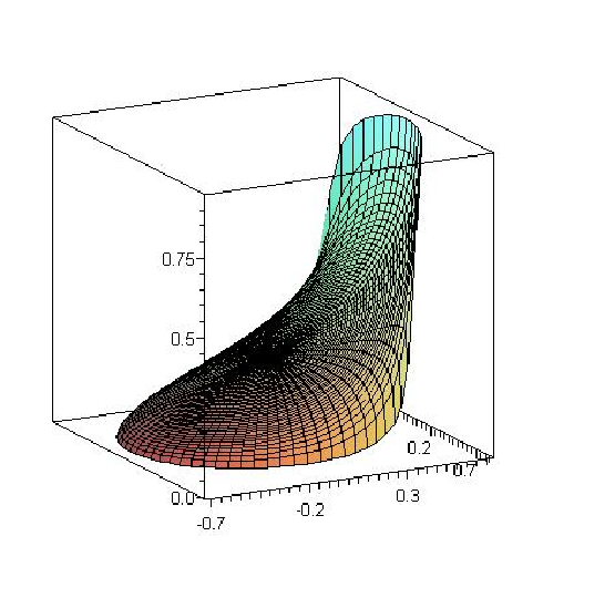
The quantity ${\tilde{q}}^{*}({\bf r},{\tilde{h}})$ is equal to $t-2s$ . This vanishes on the line shown in figure 8. The branch of the arctangent chosen in the conclusion of Theorem 3.9 varies continuously through $\pi/2$ as ${\tilde{q}}^{*}(-{\bf r},{\tilde{h}})$ varies through zero and the argument of the arctangent passes through $\pm\infty$ . The arctangent goes to zero where ${\tilde{q}}^{*}({\bf r},{\bf r})=0$ and ${\tilde{q}}^{*}({\bf r},{\tilde{h}})>0$ (the part of the boundary of the disk to the left of the vertical line) and to $\pi$ where ${\tilde{q}}^{*}({\bf r},{\bf r})=0$ and ${\tilde{q}}^{*}({\bf r},{\tilde{h}})<0$ (the part of the boundary of the disk to the right of the line). The residue ${{\rm Res}}^{(2)}$ is immediately computed from (3.8) and is equal to 1. Finally, we have $P({\bf z})=1/2$ and ${\tilde{q}}^{*}({\tilde{h}},{\tilde{h}})=-1$ . Thus, as ${\bf r}$ varies over the interior of the projective disk $B_{2}^{*}$ we have

{\mbox{\elevenss contrib}}({\bf 0})\sim\frac{1}{2\pi}\arctan\left(\frac{\sqrt{{\tilde{q}}^{*}({\bf r},{\bf r})}}{{\tilde{q}}^{*}({\bf r},{\tilde{h}})}\right)=\frac{1}{2\pi}\arctan\left(\frac{\sqrt{t^{2}-2r^{2}-2s^{2}}}{t-2s}\right)\,.

The computation for ${\bf w}=(\pi,\pi,\pi)$ is entirely analogous, leading to the same contribution but with an extra sign factor of $(-1)^{i+j+n+1}$ . We have already shown that all other contributions are of order $O(|{\bf r}|^{-1})$ . Therefore, we may sum these results to finish the proof of Theorem 4.1. A plot of this function is shown in figure 11; see [CEP, 96, Figure 2] for a contour plot of the same function. $\hfill\Box$

4.2 Cube groves

The model

After CS [04]; PS [05], we define a collection of lattice subgraphs known as cube groves. Let $L_{n}$ be the triangular lattice of order $n\geq 0$ , by which we mean the set of all triples of nonnegative integers $(r,s,t)\in({\mathbb{Z}}^{+})^{3}$ such that $r+s+t=n$ with edges between nearest neighbors (thus the degree of an interior vertex is 6). We depict this in the plane as a triangle with $n+1$ vertices in the top (zeroth) row, and so on down to 1 vertex in the $n^{th}$ row.

The cube groves of order $n$ are a subset $C_{n}$ of the subgraphs of $L_{n}$ . The set $C_{n}$ has a description where one begins with the unique cube grove of order zero, then produces sequentially groves of orders $1,2,\ldots,n$ , each produced from the previous by a “shuffle” which injects some information in a manner similar to the domino shuffling used by CEP [96] in studying and enumerating domino tilings of the Aztec diamond. The set $C_{n}$ has other, static definitions in terms of graphs that look like stacks of cubes and in terms of graphical realization of certain terms of generating functions (see PS [05]), but here we will take the shuffling procedure to define the set $C_{n}$ of order $n$ cube groves.

Define $C_{0}$ to be the singleton whose element is the one-point graph. If $T$ is a downward-pointing triangular face of $L_{n}$ , let $T^{\prime}$ be the rotation of $T$ by $180^{\circ}$ about its center. The union of the vertices of the triangles $T^{\prime}$ is a translation of the graph $L_{n+1}$ , provided that one adds in the three corner vertices of $L_{n+1}$ . The edge sets of the triangles $T^{\prime}$ are disjoint and their union is the edge set of $L_{n+1}$ , provided that one adds in the six edges adjacent to corner vertices.

Given a cube grove $G\in L_{n}$ and a downward-pointing triangular face $T$ of $L_{n}$ , let $G(T)$ be the collection of graphs on $T^{\prime}$ that have: no edges if $G$ has two edges in $T$ ; one edge if $G$ has one edge $e\in T$ , in which case the edge of $T^{\prime}$ must be the edge of $T^{\prime}$ parallel to $e$ ; two edges if $G$ has no edges in $T$ , in which case any two of the three edges of $T^{\prime}$ will do. Let $C(G)$ be the direct sum of $G(T)$ as $T$ varies over downward-pointing triangular faces of $L_{n}$ . That is, choose an element of $G(T)$ for each $T$ and take the union of these. Figure 12 shows an order 4 grove, $G$ and one of the 27 elements of $C(G)$ . Finally, let $C_{n+1}$ be the (disjoint) union of the collections $C(G)$ as $G$ runs over $L_{n}$ .

Looking at a picture of a uniformly chosen random cube grove of order 100, one sees regions of order and disorder similar to those of the Aztec Diamond.

Let $p_{n}(i,j)$ be the probability that the horizontal edge with barycentric coordinates $(i,j,n-i-j)$ is present in a uniformly chosen cube grove of order $n$ . The creation rates $E_{n}(i,j)$ may be defined in terms of the shuffling procedure but in this case they satisfy the simple relation $E_{n-1}(i,j)=\frac{3}{2}(p_{n}(i,j)-p_{n-1}(i,j))$ [PS, 05, Theorem 2]. We recall here the explicit generating function (1.4), which is derived in [PS, 05, Section 2.2]:

F(X,Y,Z)=\frac{2Z^{2}}{(1-Z)(3+3XYZ-(X+Y+Z+XY+XZ+YZ))}:=\frac{2Z^{2}}{HQ}\,.

It is quick to verify that longer factor, $Q$ , in the denominator has a quadratic cone singularity and that $F$ therefore is singular on the union of a quadratic cone with a smooth surface. The real part of this is pictured in figure 14. Application of Theorem 3.9 will yield the following result.

Theorem 4.2.

The quantity $p_{t}(r,s)$ , which is the coefficient $a_{rst}$ of $X^{r}Y^{s}Z^{t}$ in (1.4), is given asymptotically by

\frac{1}{\pi}\arctan\left(\frac{\sqrt{2(rs+rt+st)-(r^{2}+s^{2}+t^{2})}}{r+s-t}\right)

(4.3)

where the arctangent is taken in $(0,\pi)$ so that as we cross the line $t=r+s$ the arctangent varies continuously across $\pi/2$ .

The amoeba and the normal cone

All multi-indices in the generating function are nonnegative, so it is an ordinary generating function and $B$ will be the component of ${\mbox{\elevenss amoeba}}(F)^{c}$ containing the negative orthant. Again, we are chiefly interested in directions ${\bf r}$ for which ${{\bf x}_{\min}}({\bf r})={\bf 0}$ , these being the directions of non-exponential decay. The polynomial $Q$ has a single quadratic point at $(1,1,1)$ . To compute $\tan_{{{\bf x}_{\min}}}(B)$ , we intersect $B_{1}:=\{(x,y,z):z<0\}$ with the cone $B_{2}$ of hyperbolicity of $Q$ at $(1,1,1)$ . Changing to exponential coordinates via $q:=Q\circ\exp$ and computing the leading homogeneous term gives

	$\displaystyle q(x,y,z)$	$\displaystyle=$	$\displaystyle{\tilde{q}}(x,y,z)+O(\|{\bf z}\|^{3})$
	$\displaystyle\mbox{ where }\;\;\;{\tilde{q}}(x,y,z)$	$\displaystyle:=$	$\displaystyle 2xy+2xz+2yz\,.$

It follows that $B_{2}$ is the cone containing the negative orthant and bounded by $\{{\tilde{q}}=0\}$ . The dual quadratic is represented by the matrix

\left[\begin{array}[]{ccc}0&1&1\\ 1&0&1\\ 1&1&0\end{array}\right]^{-1}={\frac{1}{2}}\left[\begin{array}[]{ccc}-1&1&1\\ 1&-1&1\\ 1&1&-1\end{array}\right]\,,

hence

{\tilde{q}}^{*}(r,s,t)=rs+rt+st-{\frac{1}{2}}(r^{2}+s^{2}+t^{2})\,.

The dual cone $-B_{1}^{*}$ is the subcone of the positive orthant bounded by ${\tilde{q}}^{*}=0$ . Again, the point ${\tilde{h}}$ , which is equal to $(0,0,1)$ in the $(r,s,t)$ coordinates, lies outside this cone, and again the solutions to ${\tilde{q}}={\tilde{h}}=0$ are the solutions to $z=0=xy$ which are two distinct projective points, namely the $x$ -axis and the $y$ -axis. We could again depict this by the slice through $t=1$ , viewing $B_{2}^{*}$ as the interior of a parabola in the first quadrant, opening in the northeast direction and tangent to the axes at $(1,0)$ and $(0,1)$ , with ${\tilde{h}}$ at $(0,0)$ . It is easier to see what is going on if we change coordinates to ${\bf u}:=(1,1,1)/\sqrt{3}$ , letting $U^{\perp}$ denote the complementary space. For ${\bf r}=({\bf r}\cdot{\bf u}){\bf u}+{\bf r}^{\perp}$ with ${\bf r}^{\perp}\in U^{\perp}$ , we then have $|{\bf r}|^{2}=({\bf r}\cdot{\bf u})^{2}+|{\bf r}^{\perp}|^{2}$ , whence

|{\bf r}^{\perp}|^{2}=r^{2}+s^{2}+t^{2}-\frac{1}{3}(r+s+t)^{2}=\frac{1}{3}(r^{2}+s^{2}+t^{2})-\frac{2}{3}{\tilde{q}}^{*}(r,s,t)\,.

Thus ${\tilde{q}}^{*}(r,s,t)=0$ when $|{\bf r}|^{2}=3|{\bf r}^{\perp}|^{2}$ , or equivalently, $|{\bf r}\cdot{\bf u}|^{2}=2|{\bf r}^{\perp}|^{2}$ . Viewing projective space via the slice ${\bf r}\cdot{\bf u}=1$ , we see that ${\tilde{q}}^{*}$ vanishes on the circle centered at the origin of radius $\sqrt{1/2}$ . The projective point ${\tilde{h}}=(0,0,1)$ intersects the slice $|{\bf r}\cdot{\bf u}|=1$ at $(0,0,\sqrt{3})$ , whose projection to $U^{\perp}$ has squared norm $2$ . This is pictured in figure 15. In these coordinates, the only difference between this figure and that for the Aztec Diamond is that the distance from the origin to the point ${\tilde{h}}$ is twice the radius of the circle, rather than $\sqrt{2}$ times the radius, and the tangents subtend an arc of $120^{\circ}$ rather than $90^{\circ}$ .

Classifying the critical points

The stratification is similar to that for the Aztec Diamond generating function. There is just one singular point of $Q$ , namely $(1,1,1)$ . This is on ${\cal V}_{H}$ as well. The surfaces ${\cal V}_{H}$ and ${\cal V}_{Q}$ intersect in the set $\{x=z=1\}\cup\{y=z=1\}$ , which is smooth away from $(1,1,1)$ , leading to the following stratification.

$\displaystyle{\cal V}_{1}$	$\displaystyle:=$	$\displaystyle\{(1,1,1)\}$
$\displaystyle{\cal V}_{2}$	$\displaystyle:=$	$\displaystyle{\cal V}_{Q}\cap{\cal V}_{H}\setminus{\cal V}_{1}$
$\displaystyle{\cal V}_{3}$	$\displaystyle:=$	$\displaystyle{\cal V}_{H}\setminus({\cal V}_{1}\cup{\cal V}_{2})$
$\displaystyle{\cal V}_{4}$	$\displaystyle:=$	$\displaystyle{\cal V}_{Q}\setminus({\cal V}_{1}\cup{\cal V}_{2})$

The logarithmic gradient of $H$ is parallel to $(0,0,1)$ , which is not in ${\bf N^{*}}$ , so for ${\bf r}\in{\bf N^{*}}$ there are never any critical points on ${\cal V}_{3}$ . There are critical points on ${\cal V}_{4}$ , but we verify as before that there are only finitel many. They are smooth, so by Theorem 3.4, their contributions are $o(1)$ . On ${\cal V}_{2}$ , the logarithmic gradient of $Q$ is parallel to either $(1,0,1)$ or $(0,1,1)$ . The logarithmic gradient of $H$ is in the $t$ direction, so the span of the two logarithmic gradients is either the $r$ - $t$ plane or the $s$ - $t$ plane. Neither of these planes intersects the interior of ${\bf N^{*}}$ (the planes are tangent to ${\bf N^{*}}$ at the projective points $(1,0,1)$ and $(0,1,1)$ respectively). The for ${\bf r}$ interior to ${\bf N^{*}}$ , there are no contributions from ${\cal V}_{2}$ ; it remains to compute the contribution from ${\cal V}_{1}$ .

Computing the estimate

Completing the computation as in the Aztec case, we evaluate ${{\rm Res}}^{(2)}$ using (3.8) but switching the roles of $x$ and $z$ because only the $z$ -derivative of ${\tilde{h}}$ is non-vanishing. This gives ${{\rm Res}}^{(2)}={\frac{1}{2}}$ . With $P=2Z^{2}$ , and only one contributing point ${\bf w}=(0,0,0)$ , we have ${\tilde{q}}^{*}({\bf r},{\tilde{h}})=(r+s-t)/2$ and ${\tilde{q}}^{*}({\tilde{h}},{\tilde{h}})=-1/2$ , whence Theorem 3.9 gives

	$\displaystyle a_{\bf r}$	$\displaystyle\sim$	$\displaystyle\frac{1}{\pi}\arctan\left(\frac{\sqrt{{\frac{1}{2}}{\tilde{q}}^{*}({\bf r},{\bf r})}}{(r+s-t)/2}\right)$
		$\displaystyle=$	$\displaystyle\frac{1}{\pi}\arctan\left(\frac{\sqrt{2(rs+rt+st)-(r^{2}+s^{2}+t^{2})}}{r+s-t}\right)\,,$

finishing the proof of Theorem 4.2. $\hfill\Box$

4.3 Two-dimensional quantum random walk

The model

We begin with a brief review on one-dimensional quantum random walk (QRW). In the classical simple random walk, the law at time $n$ is a probability measure on ${\mathbb{Z}}$ and the evolution operator on this law is $(1/2)\sigma_{+}+(1/2)\sigma_{-}$ , where $\sigma_{+}$ is the right-shift operator $\sigma_{+}\mu(n)=\mu(n-1)$ and $\sigma_{-}$ is the left-shift operator $\sigma_{-}\mu(n)=\mu(n+1)$ . In the quantum world, the law at time $n$ is given by the values of $|\psi(n)|^{2}$ where the wave function $\psi$ is not a positive unit vector in $L^{1}({\mathbb{R}})$ but rather a unit vector in $L^{2}({\mathbb{C}})$ . Evolution operators must be unitary. While the shifts $\sigma_{\pm}$ are unitary, linear combinations of these such as $(1/2)\sigma_{+}+(1/2)\sigma_{-}$ are not.

An idea for constructing a quantum simple random walk, apparently due to Mey [96], is to enlarge the space to $:={\mathbb{Z}}\times\{U,D\}$ , adding a hidden “spin” variable. To take a step of the random walk, first the spin is randomized, then all particles with spin up move one step right and all particles with spin down move one step left. A number of choices are available for the operator that executes the evolution of spins. One common choice is the Hadamard coin-flip, $B:=\displaystyle{\frac{1}{\sqrt{2}}\left(\begin{array}[]{cc}1&1\\ 1&-1\end{array}\right)}$ . The terminology reflects the fact that the matrix is a multiple of an orthogonal matrix with $\pm 1$ entries, these being known as Hadamard matrices. Under this operator, either state $(1,0)$ or $(0,1)$ becomes an equal mix of U and D states. Let $A$ be the operator which maps state $(n,U)$ to $(n+1,U)$ and $(n,D)$ to $(n-1,D)$ . If we begin in state $(0,U)$ , then do ${\cal S}:=A\circ B$ , the particle is in an equal mix of states $(1,U)$ and $(-1,D)$ . If we measure the position, we will have executed a step of QRW.

The $n$ -step simple random walk is defined to be the operator ${\cal S}^{n}:=(AB)^{n}$ . If the position if this is measured at time $n$ , the probability of being at position $k$ is $|{\cal S}^{n}(k,U)|^{2}+|{\cal S}^{n}(k,D)|^{2}$ . Since no measurement is made until time $n$ , the various possible coin-flips and movements interfere, both positively and negatively, and the result is somewhat complicated. The analyses in NV [00]; ABN+ [01] show that unlike classical simple random walk, QRW spreads out linearly, with location distributed over the interval $[-n/\sqrt{2},n/\sqrt{2}]$ ; see also the review article Kem [05].

To define a two-dimensional QRW, we need a four-fold auxiliary state. Denote these four states by $\{N,S,E,W\}$ . Any $4\times 4$ unitary matrix may be used for the quantum coin-flip. The Hadamard matrix

U:=\frac{1}{2}\left(\begin{array}[]{cccc}1&-1&-1&-1\\ -1&1&-1&-1\\ -1&-1&1&-1\\ -1&-1&-1&1\end{array}\right)

is known (http://www.santafe.edu/ moore/gallery.html) as the Hadamard quantum coin-flip. N.B.: This is different from the Hadamard QRW in GJS [04], which also uses a Hadamard matrix, namely the tensor product of two copies of the one-dimensional Hadamard matrix. A step of the two-dimensional Hadamard QRW is the product $AU$ where $A$ maps $((r,s),N)$ to $((r,s+1),N)$ , and so forth. The following generating function for the probability amplitudes of a QRW in any dimension with any quantum coin-flip matrix is given in [BP, 07, Proposition 3.1]. Let $M$ be obtained from $U$ by multiplying the first row by $XZ$ , the second by $YZ$ , the third by $X^{-1}Z$ and the fourth by $Y^{-1}Z$ . We consider the rows and columns of $M$ as indexed by the ordered quadruple $(E,N,W,S)$ . Then an entry of $M^{t}$ such as $(M^{t})_{N,E}$ counts the number of $t$ -step paths from $N$ to $E$ , weighted by $M$ : the $X^{r}Y^{s}Z^{t}$ coefficient of this is the wave function at position $((r,s),N)$ and time $t$ starting from $((0,0),N)$ . Summing in $t$ shows that the components of $(I-M)^{-1}=\sum M(r,s,t)X^{r}Y^{s}Z^{t}$ are the generating functions for the wave function at all positions and times: each $M(r,s,t)$ is a matrix, whose $(\xi,\eta)$ -entry is the generating function $\sum_{r,s,t}c(\xi,\eta;r,s,t)X^{r}Y^{s}Z^{t}$ where $c(r,s,t)$ is the probability amplitude, starting from state $((0,0),\xi)$ at time zero, of being in state $((r,s),\eta)$ at time $t$ .

The entries of $(I-M)^{-1}$ have denominator $(1-Z^{2})Q$ where

Q:=1-2\frac{X+X^{-1}+Y+Y^{-1}}{4}Z+Z^{2}\,.

We recognize the same polynomial factor that occurred in the Aztec denominator. We know of no reason for this coincidence. This particular QRW is somewhat special, both because of the occurrence of a quadratic point and because the denominator is reducible. The numerators in the first row are half of the following.

$\displaystyle P_{1}$	$\displaystyle=$	$\displaystyle 2-(Y+Y^{-1}+X^{-1})Z+Z^{3}$
$\displaystyle P_{2}$	$\displaystyle=$	$\displaystyle XZ-(1+Y^{-1}X)Z^{2}+Y^{-1}Z^{3}$
$\displaystyle P_{3}$	$\displaystyle=$	$\displaystyle XZ-(YX+Y^{-1}X)Z^{2}+XZ^{3}$
$\displaystyle P_{4}$	$\displaystyle=$	$\displaystyle XZ-(1+XY)Z^{2}+YZ^{3}$

The chiralities $\{N,E,S,W\}$ and the location $(i,j)$ are simultaneously measurable, so the probability of a QRW started at $((0,0),N)$ to be found at $(r,s)$ at time $t$ is the sum over $1\leq k\leq 4$ of $|{\cal C}_{r,s,t}P_{k}|^{2}$ , the squared moduli of the probability amplitudes of going from $((0,0),N)$ to $((r,s),\xi)$ in time $t$ for $\xi\in\{N,E,S,W\}$ .

Results

A number of different two-dimensional QRW’s are analyzed in BBBP [08]. In these examples, the variety defined by the common denominator $\det(I-M)$ of the entries of $(I-M)^{-1}$ turns out to be smooth, and amplitudes may be computed from Theorem 3.4. Figure 16 shows an intensity plot for a quantum walk whose unitary matrix $U$ was generated at random without any symmetries.

The feasible region, where the probability amplitudes do not decay exponentially, is a well defined region of irregular shape. It is the image of the torus under the logarithmic Gauss map. The region is determined by the denominator $\det(I-M)$ of the the spacetime generating function.

We now restrict our attention to the Hadamard QRW. The methods of BBBP [08] did not suffice to analyze this QRW because of the quadratic point and the fact that the denominator $(1-Z^{2})Q$ is not irreducible. Two of the factors are binomials $(1\pm Z)$ and the third factor, $Q$ , has quadratic points at $\pm(1,1,1)$ , each of which is on one of the binomial varieties. The time-200 intensity plot for this QRW is shown in Figure 17, where the $x$ and $y$ axes are rescaled spatial variables $(r/t,s/t)$ , or in other words, velocities.

The feasible region is evidently highly symmetric. Within the feasible region, however, there is asymmetric variation in the intensities. This is due to the somewhat arbitrary choice of starting and ending states, which produce the numerators $P_{1},P_{2},P_{3}$ and $P_{4}$ , none of which possesses rotational symmetry in the $X$ - $Y$ plane. The following result rigorously establishes the picture in Figure 17.

Theorem 4.3 (feasible region for the two-dimensional Hadamard QRW).

When the velocity is outside the closed disk of radius $\sqrt{1/2}$ the amplitudes decay exponentially. Inside this disk, except possibly at the center, the amplitudes do not decay exponentially and are instead $\Theta(t^{-1})$ .

Remark.

It will turn out that the dominant contribution to the asymptotics of the probability amplitudes everywhere except possibly at the center and boundary are controlled by smooth points rather than by the two quadratic points. The reason we include this example in the present paper is that controlling the estimate at the quadratic points will require the big-O lemma.

The amoeba and the normal cone

Denoting $H_{1}=1-Z,H_{-1}=1+Z$ , we have $F_{j}=P_{j}/(QH_{1}H_{-1})$ , which is in the format of the quadratic point hypotheses with $\eta=2$ . The origin is on the boundary of a component $B$ of the complement of ${\mbox{\elevenss amoeba}}(QH_{1}H_{-1})$ containing the negative $z$ -axis. As before, the cone $\tan_{\bf 0}(B)$ is the intersection of components of ${\mbox{\elevenss amoeba}}(Q)^{c}$ , ${\mbox{\elevenss amoeba}}(H_{1})^{c}$ , and ${\mbox{\elevenss amoeba}}(H_{-1})^{c}$ . The latter two are just the halfspaces $\{(x,y,z):z<0\}$ , which are equal and contain the component $B_{0}:=\{(x,y,z):z<0,\;z^{2}>(x^{2}+y^{2})/2$ , which we recognize from the Aztec Diamond example. Therefore, $B=B_{0}$ and $B^{*}=\{t^{2}>2(r^{2}+s^{2})\}$ as in Section 4.1. An immediate consequence is that the amplitudes decay exponentially for velocities in directions outside the disk of radius $\sqrt{1/2}$ . This proves the first part of Theorem 4.3.

To understand the amplitudes inside the disk, we will first use the big-O lemma to show that the contribution from the quadratic points is $O(t^{-2})$ everywhere except possibly at the center (zero velocity). We will then deduce from Theorem 3.4 that the contribution from the smooth points anywhere in the range of the logarithmic Gauss map is $\Theta(t^{-1})$ . Finally, we will show that the range of the logarithmic Gauss map is precisely the disk of radius $\sqrt{1/2}$ .

Classification of critical points

The intersection of ${\cal V}_{Q}$ with ${\cal V}_{H_{j}}$ is the set

\left\{Z=j=\frac{X+X^{-1}+Y+Y^{-1}}{4}\right\}\,.

The varieties ${\cal V}_{H_{1}}$ and ${\cal V}_{H_{-1}}$ do not intersect. We therefore stratify by

$\displaystyle{\cal V}_{1}$	$\displaystyle:=$	$\displaystyle\{(1,1,1),(-1,-1,-1)\}$
$\displaystyle{\cal V}_{2+}$	$\displaystyle:=$	$\displaystyle{\cal V}_{Q}\cap{\cal V}_{H_{1}}\setminus{\cal V}_{1}$
$\displaystyle{\cal V}_{2-}$	$\displaystyle:=$	$\displaystyle{\cal V}_{Q}\cap{\cal V}_{H_{-1}}\setminus{\cal V}_{1}$
$\displaystyle{\cal V}_{3+}$	$\displaystyle:=$	$\displaystyle{\cal V}_{H_{1}}\setminus({\cal V}_{1}\cup{\cal V}_{2+})$
$\displaystyle{\cal V}_{3-}$	$\displaystyle:=$	$\displaystyle{\cal V}_{H_{-1}}\setminus({\cal V}_{1}\cup{\cal V}_{2-})$
$\displaystyle{\cal V}_{4}$	$\displaystyle:=$	$\displaystyle{\cal V}_{Q}\setminus({\cal V}_{1}\cup{\cal V}_{2\pm}\cup{\cal V}_{3\pm})$

Again, we are interested in the region of non-exponential decay, where ${{\bf x}_{\min}}={\bf 0}$ ; checking where the strata intersect the unit torus, we find that the strata ${\cal V}_{2\pm}$ do not intersect the unit torus. The strata ${\cal V}_{3\pm}$ intersect the unit torus on the set $\{|X|=|Y|=Z=1\}$ , and the logarithmic gradient is always in the $t$ direction. The factors $H_{1}$ and $H_{-1}$ cause this direction to be obstructed and we are therefore not able to say anything about asymptotics in the $(0,0,t)$ direction. This direction corresponds to the bright spot in the middle of the amplitude intensity plot in figure 17, where there appears to be a bound state (probability amplitude for being precisely at the origin does not decay with time).

Contributions from ${\cal V}_{1}$ occur for ${\bf r}$ interior to ${\bf N^{*}}$ . The big-O estimate, Lemma 5.9 below, allows us to bound the magnitude of these contributions. We first compute the homogeneous degree of $F$ at the point $(1,1,1)$ . The factor $1/Q$ has degree $-2$ here, the factor $1/H_{1}$ has degree $-1$ , and the factor $1/H_{2}$ has degree zero. The numerators $P_{j}$ vanish to order two at $(1,1,1)$ for all $1\leq j\leq 4$ . We therefore have $\deg(F,(1,1,1))=\deg(f,(0,0,0))=2-2-1=-2$ . Applying the lemma, we find that for the quadratic point ${\bf w}={\bf 0}$ , we have ${\mbox{\elevenss contrib}}({\bf w})=O(t^{-2})$ , proving the second part of Theorem 4.3.

It is shown in Bra [07], that the projective range of the logarithmic Gauss map is the disk of radius $\sqrt{1/2}$ , but because this is an unpublished Masters thesis, we will give an alternative derivation. Assuming this for the moment, it is evident that the contribution from the smooth points is $\Theta(t^{-1})$ . If more detail is desired, one can follow Brady Bra [07] to verify periodicity and the visually obvious Moire patterns as follows. Brady shows that for each ${\bf r}$ interior to ${\bf N^{*}}$ , there are precisely four smooth critical points on the unit torus, a conjugate pair and its negative: ${\bf Z}(\hat{{\bf r}}),\overline{{\bf Z}}(\hat{{\bf r}}),-{\bf Z}(\hat{{\bf r}}),-\overline{{\bf Z}}(\hat{{\bf r}})$ . Denoting $\log{\bf Z}(\hat{{\bf r}})={\bf z}=i{\bf w}$ , Theorem 3.4 tells us that

{\mbox{\elevenss contrib}}({\bf w})\sim C(\hat{{\bf r}})|{\bf r}|^{-1}\exp(-i{\bf r}\cdot{\bf w})

where the magnitude of $C(\hat{{\bf r}})$ is proportional to the $-1/2$ -power of the complex curvature of $\log{\cal V}_{Q}$ at ${\bf z}$ . Adding this to the contribution from $\overline{{\bf Z}}$ , namely ${\mbox{\elevenss contrib}}(-{\bf w})$ , we obtain a quantity whose magnitude is $2\cos\theta({\bf r})$ times the magnitude of ${\mbox{\elevenss contrib}}({\bf w})$ , where $\theta$ is the argument of ${\mbox{\elevenss contrib}}({\bf w})$ ; note that $\theta$ differs from ${\bf r}\cdot{\bf w}$ by $\pi/4$ because the curvature is complex and its $-1/2$ power has argument $-\sigma\pi/4$ , where $\sigma$ is the signature of ${\tilde{q}}$ , which in our case is $1-2=-1$ ; see [BBBP, 08, Section 2.3] for details on the phase of the curvature. Adding the contribution from the negatives of these two points kills the terms for which $r+s+t$ is odd and doubles the even terms. This corresponds to periodicity of the walk. For fixed $t$ , the phase term $\cos\theta({\bf r})$ varies rapidly (with period of order 1). Ignoring the Moiré pattern resulting from this term, the probabilities are of order $t^{-2}$ (amplitudes are of order $t^{-1}$ ) and are spread over the disk $r^{2}+s^{2}=t^{2}/2$ , which is the slice of the normal cone at the fixed value of $t$ . We now finish the proof of Theorem 4.3 by showing that the range of the logarithmic Gauss map on ${\cal V}_{4}$ is the disk of radius $\sqrt{1/2}$ .

Proof of the remainder of Theorem 4.3: Let $(x,y,z)$ be a point on ${\cal V}_{4}\cap{\mathbb{T}}^{3}$ , where ${\mathbb{T}}^{3}$ denote the 3-torus $\{|x|=|y|=|z|=1\}$ . The projective logarithmic Gauss map is the map $\gamma_{\mathbb{P}}$ that takes $(x,y,z)$ to the projective point $(a|b|c)$ where $(a,b,c)$ is the gradient of $Q\circ\exp$ at $\log(x,y,z)$ . We represent the class $(a|b|c)$ by the normalized vector $(a/c,b/c)\in{\mathbb{R}}^{2}$ . Because the domain is a subset of ${\mathbb{T}}^{3}$ we may use polar coordinates $x=\exp(i\phi),y=\exp(i\psi),z=\exp(i\theta)$ . In these coordinates, ${\cal V}\cap{\mathbb{T}}^{3}$ is given by

\Sigma=\left\{2\cos(\theta)=\cos(\phi)+\cos(\psi)\right\}\,,

where $(\phi,\psi,\theta)\in{\mathbb{T}}^{3}$ . The Gauss map takes $(\phi,\psi,\theta)\in\Sigma$ to $-(\sin(\phi),\sin(\psi),-2\sin(\theta))=:(a,b,c)$ . A simple computation shows that $c^{2}/2=a^{2}+b^{2}+(\cos(\phi)-\cos(\psi))^{2}/2$ , whence the image of the Gauss map is contained in the two space-like cones $\{c^{2}/2\geq a^{2}+b^{2}\}$ , and its projectivization is contained in the disk $D:=\{r^{2}+s^{2}\leq 1/2\}$ .

We first show that the boundary of the disk $D$ belongs to the closure of the range of $\gamma_{\mathbb{P}}$ . Near $(\phi,\psi,\theta)=(0,0,0)$ , the surface $\Sigma$ is given by

\Sigma=\{\theta^{2}-\frac{\phi^{2}}{2}-\frac{\psi^{2}}{2}+R_{3}(\theta,\phi,\psi)=0\}\,,

where $R_{3}$ denotes the terms of order three and higher in local coordinates. Therefore the projectivization of Gauss map takes vicinity of the point $(0,0,0)$ to vicinity of the image of the projectivization of the Gauss map of the conic $\{\theta^{2}-\phi^{2}/2-\psi^{2}/2=0\}$ , which is the boundary of $D$ .

To prove, finally, that all of the interior of $D$ is in the range of the projectivization of the Gauss map, we notice that were that not the case, this mapping would have some critical values in the interior of $D$ . Critical points of the projectivization of the Gauss map correspond to the parabolic points of $\Sigma$ (points where at least one of the principal curvatures of the second quadratic form of $\Sigma$ vanishes). To find those, we use the standard trick characterizing the locus of the parabolic points of the surface given by $\{f=0\}$ by the equation

\langle df,\det H\cdot H^{-1}df\rangle\,,

where $H$ is the Hessian of $f$ ; $df$ is the gradient (and the matrix $\det H\cdot H^{-1}$ is the adjunct matrix to $H$ ). In our case, quick computation implies that the parabolic points of $\Sigma$ lie on the intersection of $\Sigma$ with

\left\{\cos(\phi)\cos(\psi)\cos(\theta)\left(\frac{2\sin(\theta)^{2}}{\cos(\theta)}-\frac{\sin(\phi)^{2}}{\cos(\phi)}+\frac{\sin(\psi)^{2}}{\cos(\psi)}\right)=0\right\}\,,

which, as again a short computation shows, yields critical values only on the boundary of $D$ . Hence the interior of $D$ is contained in the range of $\gamma_{\mathbb{P}}$ . $\hfill\Box$

4.4 Friedrichs-Lewy-Szegö graph polynomials

In the the study of a discretized time-dependent wave equation in two spatial dimensions, Friedrichs and Lewy required a nonnegativity result for the coefficients of $Q^{-1}$ where $Q(X,Y,Z):=(1-X)(1-Y)+(1-X)(1-Z)+(1-Y)(1-Z)$ . To solve this problem, Szegö Sze [33] showed that the coefficients of $Q^{-\beta}$ are nonnegative for all $\beta\geq 1/2$ . Scott and Sokal SS [06] later observed that $Q$ is a special case of a spanning tree polynomial of a graph. They proved a generalization of Szegö’s result to all series-parallel graphs. Their results are proved via the stronger property of complete monotonicity and are related to the half-plane property. In order to investigate whether these results might hold for the polynomials of a larger class of graphs, Scott and Sokal needed a means of checking the asymptotics of the coefficients: asymptotic nonnegativity is a necessary condition for term-by-term nonnegativity. We will apply Theorem 3.7 to obtain:

Theorem 4.4.

Fix $\beta>1/2$ and let $\sum_{\bf r}a_{\bf r}{\bf Z}^{\bf r}$ be a Taylor expansion for $Q^{-\beta}$ . Then

a_{\bf r}\sim\frac{4^{1-\beta}}{\sqrt{\pi}\Gamma(\beta)\Gamma(\beta-1/2)}(2rs+2rt+2st-r^{2}-s^{2}-t^{2})^{-1/2}

as ${\bf r}$ varies over compact subsets of the cone $2(rs+rt+st)>r^{2}+s^{2}+t^{2}$ .

The simplest nontrivial case in which asymptotics may be worked out is the one above. Szegö’s 1933 proof of nonnegativity was, according to Scott and Sokal, “surprisingly indirect, exploiting Sonine-type integrals for products of Bessel functions.” It is evident that asymptotics in this case may be derived directly from Theorem 3.7. We remark that the connection between these coefficients and harmonic analysis of symmetric cones is known to Scott and Sokal, who exploit the connection and cite several results on the subject from the sources FK [94]; Ish [00].

Proof of Theorem 4.4: We first check that ${\bf 0}$ is on the boundary of the component $B$ of ${\mbox{\elevenss amoeba}}(Q)^{c}$ corresponding to the ordinary power series $1/Q=\sum_{\bf r}a_{\bf r}{\bf Z}^{\bf r}$ . This follows if we show that $Q(X,Y,Z)\neq 0$ for $X,Y,Z$ in the open unit disk. To see this, let $D_{1}$ denote the open unit disk, let $D_{2}$ denote the open disk $\{|z-1|<1\}$ , and let $D_{3}$ denote the halfspace $\{z:{\rm Re\,}\{z\}>1/2\}$ . The set $D_{3}$ is the image under $z\mapsto 1/z$ of $D_{2}$ and $D_{2}=1-D_{1}$ . Therefore, $Q$ has a zero on the open unit polydisk $D_{1}^{3}$ if and only if $XY+YZ+ZX$ has a zero on $D_{2}^{3}$ ; this is equivalent to $1/X+1/Y+1/Z$ having a zero on $D_{2}^{3}$ which is equivalent to $X+Y+Z$ having a zero on $D_{3}^{3}$ . This is impossible because $D_{3}$ is contained in the open right half-plane.

Composing with the exponential, then taking the leading homogeneous part, we obtain

{\tilde{q}}=\mbox{\elevenss hom}(Q\circ\exp,{\bf 0})=xy+xz+yz\,.

We recognize this as half the quadratic factor in Section 4.2. Therefore ${\tilde{q}}^{*}$ is twice what is was there:

{\tilde{q}}^{*}(r,s,t)=2(rs+rt+st)-(r^{2}+s^{2}+t^{2})\,.

Let $P(Z)\equiv 1$ . Recalling that $M$ is chosen so that the matrix for the quadratic form is $(M^{-1})^{T}DM^{-1}$ , we see that the determinant of $M$ is $\det(q)^{-1/2}$ ; plugging in the matrix $\displaystyle{\left[\begin{array}[]{ccc}0&\frac{1}{2}&\frac{1}{2}\\ \frac{1}{2}&0&\frac{1}{2}\\ \frac{1}{2}&\frac{1}{2}&0\end{array}\right]}$ for $q$ we obtain $|M|=2$ . Thus, for $\beta>1/2$ , equation (3.5) gives

a_{\bf r}\sim\frac{4^{1-\beta}}{\sqrt{\pi}\Gamma(\beta)\Gamma(\beta-1/2)}(2rs+2rt+2st-r^{2}-s^{2}-t^{2})^{-1/2}\,,

finishing the proof. $\hfill\Box$

To check this estimate, let $r=s=t=50$ and compute

a_{\bf r}\approx\frac{4^{1-\beta}7500^{\beta-3/2}}{\sqrt{\pi}\,\Gamma(\beta)\,\Gamma(\beta-1/2)}\approx 0.000222832\ldots

when $\beta=3/4$ . We then use Maple to crank out the true value of $a_{50,50,50}$ which is a rational number near $0.000223464$ , for a relative error of around $1/400$ .

4.5 Super ballot numbers and multiset permutations

Gessel Ges [92] defines the super ballot numbers by

g(n,k,r):=\frac{(k+2r)!\,(2n+k-1)!}{(k-1)!\,r!\,n!\,(n+k+r)!}\,.

These are a generalization of the ballot numbers $\displaystyle{\frac{k}{2n+k}{2n+k\choose n}}$ (obtained by setting $r=0$ ), which are in turn a generalization of the Catalan numbers (set $k=1$ ). The Catalan number and the ballot numbers are integral and have combinatorial interpretations. Gessel shows that the super ballot numbers are integers as well and sets as a goal to find a combinatorial interpretation.

After re-indexing via $B(a,b,c):=g(a,b-a-c,c)$ for $b>a+c$ , one may extend this definition to all nonnegative $(a,b,c)$ and obtain a generating function

F(X,Y,Z)=\sum_{a,b,c\geq 0}B(a,b,c)X^{a}Y^{b}Z^{c}=\frac{1-2X}{\sqrt{1-4XZ}}\,G(X,Y,Z)

where $G$ is the generating function from equation (1.7). The coefficients $N(a,b,c)$ of $G$ are of independent interest. They satisfy a similar recurrence to the super ballot numbers $B(a,b,c)$ but with different boundary conditions. The numbers $\{N(a,b,c)\}$ were shown in Ask [75] to have nonnegative coefficients. They count a difference of cardinalities of multi-set permutations AI [76]. Gessel goes on to find several more identities involving these numbers and their generating functions, but no asymptotics are derived. We will use Corollary 3.8 to obtain the following asymptotic estimate.

Theorem 4.5.

The numbers $N(a,b,c)$ are estimated asymptotically by

N(a,b,c)\sim 2^{a+b+c}\frac{4}{2\pi}(2ab+2ac+2bc-a^{2}-b^{2}-c^{2})^{-1/2}

uniformly on compact subcones of ${\bf N^{*}}=\{(a,b,c):2(ab+ac+bc)>a^{2}+b^{2}+c^{2}\}$ .

Our motivation for analyzing the numbers $\{N(a,b,c)\}$ is admittedly “because we can”. The coefficients of $F$ are of greater interest than the coefficients of $G$ , but the fractional power on the non-quadratic term takes this problem beyond the main results of this paper. The deformations in Section 5 still apply, but the further analysis in Section 6.6 via Leray cycles does not work when this factor is algebraic rather than a simple pole. We therefore do not state detailed asymptotics for $F$ , reserving this for future work.

Let $Q(X,Y,Z):=2-X-Y-Z+XYZ$ , so that $2/Q$ is the ordinary power series generating function for $2^{-a-b-c}N(a,b,c)$ . It is easy to check (e.g., via Gröbner bases) that $Q$ and its gradient vanish simultaneously exactly at the point ${\bf 1}$ . We have $q:=Q\circ\exp=xy+yz+xz+O(|(x,y,z)|^{3}$ , whose homogeneous part (at ${\bf 0}$ ) is given by ${\tilde{q}}=xy+yz+xz$ . Again,

{\tilde{q}}^{*}(r,s,t)=2(rs+rt+st)-(r^{2}+s^{2}+t^{2})

and $|M|=2$ .

There is a component $B$ of ${\mbox{\elevenss amoeba}}(Q)^{c}$ containing a translate of the negative orthant (corresponding to the ordinary power series expansion); let us check that ${\bf 0}\in\partial B$ . Proceeding as in Section 4.4, it suffices to verify that $Q$ has no zero in the open unit polydisk $D_{1}$ , which is equivalent to checking that $Q({\bf 1}+{\bf Z})$ has no zero in $-D_{2}^{3}$ where $D_{2}=\{z:|z+1|<1\}$ . We have

Q({\bf 1}+{\bf Z})=XYZ+XY+XZ+YZ=XYZ\left(1+\frac{1}{X}+\frac{1}{Y}+\frac{1}{Z}\right)\,,

whence this is further equivalent to $1+X+Y+Z$ having no zero in $-D_{3}^{3}$ , where $-D_{3}$ is the halfplane $\{z:{\rm Re\,}\{z\}<-1/2\}$ . This is obvious, because the real part of $X+Y+Z$ is bounded above by $-3/2$ on $D_{3}^{3}$ .

We now apply Corollary 3.8 to obtain the asymptotics of $2^{-a-b-c}N(a,b,c)$ inside the cone ${\bf N^{*}}$ , these asymptotics being exponentially small outside ${\bf N^{*}}$ . Letting $P(Z)\equiv 2$ , we plug $P$ , $|M|$ and ${\tilde{q}}^{*}$ into (3.7) to obtain the leading term asymptotics for the coefficients of $2/Q$ , which gives the expression in Theorem 4.5 and finishes the proof. As an example, if $a=1,b=20,c=30$ , then the approximation yields $N(a,b,c)\approx 2.595\times 10^{16}$ while the actual value of $N(10,20,30)$ to three decimal places is $2.547\times 10^{16}$ . $\hfill\Box$

5 Homotopy constructions

Recall from the heuristic discussion following (1.8) that moving the chain of integration in (1.2) to the torus ${\rm ReLog\,}^{-1}({{\bf x}_{\min}})$ is not enough. Our goal in this section is to construct homotopies moving this chain of integration, within the domain of holomorphy of the integrand (but not within the domain of convergence of the Laurent series) to a different chain on which the maximum modulus of the integrand is small except in a neighborhood of ${\mbox{\elevenss crit}}({\bf r})$ . While the Morse theoretic methods of GM [88] are in principle constructive, we follow ABG [70], taking advantage of hyperbolicity in order to produce vector fields along which chains may be shifted.

5.1 Vector fields

Let $T_{\mathbb{R}}:=({\mathbb{R}}/2\pi{\mathbb{Z}})^{d}$ denote the $d$ -dimensional flat torus. Given a Laurent polynomial $F$ and a component $B$ of the complement of ${\mbox{\elevenss amoeba}}(F)$ , pick a unit vector $\hat{{\bf r}}$ in the interior of the convex dual $-B^{*}$ . We suppose that ${\bf r}$ is a proper direction for $B$ . Let

U=\bigcup_{{\bf w}\in{\mbox{\elevenss W}}({\bf r})}U_{\bf w}

(5.1)

be the disjoint union of neighborhoods of each ${\bf w}\in{\mbox{\elevenss W}}({\bf r})$ , where ${\mbox{\elevenss W}}({\bf r})$ are the logarithmic critical sets from Definition 2.21.

Lemma 5.1 (Vector field away from the critical set).

Let $F$ be a Laurent polynomial with $f:=F\circ\exp$ , let $B$ be a component of ${\mathbb{R}}^{d}\setminus{\mbox{\elevenss amoeba}}(f)$ , and let $\hat{{\bf r}}$ be a unit vector in the interior of the convex dual $-B^{*}$ . Suppose $-\hat{{\bf r}}\cdot{\bf x}$ is minimized at a unique ${{\bf x}_{\min}}$ in $\partial B$ and define the neighborhood $U$ of ${\mbox{\elevenss W}}({\bf r})$ as in (5.1). Then there is a smooth vector-valued function $\eta_{U^{c}}:T_{\mathbb{R}}\setminus U\to{\mathbb{R}}^{d}$ such that:

(i)

$\eta_{U^{c}}({\bf y})\in{\bf K}^{f,B}(\exp({{\bf x}_{\min}}+i{\bf y}))$ ;
(ii)

$\hat{{\bf r}}\cdot\eta_{U^{c}}({\bf y})=1$ for all ${\bf y}\in T_{\mathbb{R}}\setminus U$ .

Proof: First, for each ${\bf y}\notin U$ , we will find a neighborhood ${\cal N}_{\bf y}$ and a vector ${\bf v}_{\bf y}$ such that $\eta_{U^{c}}\equiv{\bf v}_{\bf y}$ fulfills $(i)$ – $(ii)$ on ${\cal N}_{\bf y}$ .

Fix ${\bf y}\notin U$ . If $f({{\bf x}_{\min}}+i{\bf y})\neq 0$ then choose a neighborhood ${\cal N}_{\bf y}$ of ${\bf y}$ in ${\mathbb{R}}^{d}$ such that for ${\bf v}\in{\cal N}_{\bf y}$ , the quantity $f({{\bf x}_{\min}}+i{\bf v})$ does not vanish. Choose ${\bf v}_{\bf y}$ with $\hat{{\bf r}}\cdot{\bf v}_{\bf y}=1$ .

Alternatively, suppose that $f({{\bf x}_{\min}}+i{\bf y})=0$ . By Proposition 2.12, the homogeneous part, call it $A_{\bf y}$ , of the function ${\bf v}\mapsto f({{\bf x}_{\min}}+i{\bf y}+{\bf v})$ is real and hyperbolic, and by Proposition 2.8, there is a cone $K$ of hyperbolicity containing $\tan_{{{\bf x}_{\min}}}(B)$ . Also by the first part of Proposition 2.22, there is some ${\bf v}_{\bf y}\in K$ with $\hat{{\bf r}}\cdot{\bf v}_{\bf y}=1$ . By semi-continuity (part $(i)$ of Corollary 2.15), ${\bf v}_{\bf y}\in{\bf K}(\exp({{\bf x}_{\min}}+i{\bf u}))$ for every ${\bf u}$ in some neighborhood ${\cal N}_{\bf y}$ of ${\bf y}$ .

The collection $\{{\cal N}_{\bf w}:{\bf w}\notin U\}$ covers $U^{c}$ ; shrink it slightly if necessary so that the closure of its union does not intersect ${\mbox{\elevenss W}}({\bf r})$ . We may (shrinking some of the $\eta_{\bf w}$ slightly if necessary) choose a finite subcover $\{{\cal N}_{\bf w}:{\bf w}\in\Xi\}$ whose union has closure disjoint from ${\mbox{\elevenss W}}({\bf r})$ . Choose a partition of unity $\{\psi_{\bf w}:{\bf w}\in\Xi\}$ subordinate to the subcover. Define

\eta_{U^{c}}({\bf y}):=\sum_{{\bf w}\in\Xi}\psi_{\bf w}({\bf y}){\bf v}_{\bf w}({\bf y})\,.

Now $(i)$ is satisfied by convexity and $(ii)$ is satisfied by linearity. $\hfill\Box$

Corollary 5.2 (Vector field defined everywhere).

Under the conditions of Lemma 5.1 there is a smooth vector field $\eta$ satisfying

	$\displaystyle\eta({\bf y})$	$\displaystyle\in$	$\displaystyle{\bf K}^{f,B}(\exp({\bf x}+i{\bf y}))\,;$		(5.2)
	$\displaystyle\hat{{\bf r}}\cdot\eta({\bf y})$	$\displaystyle=$	$\displaystyle 1\;\;\mbox{ on }U^{c}\,.$		(5.3)

Proof: Let $\eta_{\bf w}:U_{\bf w}\to{\mathbb{C}}^{d}$ be any map for which $\eta_{\bf w}({\bf y})\in{\bf K}^{{\overline{f}},B}(\exp({\bf x}+i{\bf y}))$ . To see that we may choose such a map smoothly, note that the constant map $\eta_{\bf w}({\bf y})\equiv{\bf v}$ is such a map whenever ${\bf v}\in\tan_{\bf x}(B)$ . The reason for allowing a general function $\eta_{\bf w}$ in place of a constant is that later we will use (5.4) with functions $\eta_{\bf w}$ tailored to more specific needs. The collection $\{{\cal N}_{\bf w}:{\bf w}\in\Xi\}\cup\{U_{\bf w}:{\bf w}\in{\mbox{\elevenss W}}(\hat{{\bf r}})\}$ covers $T_{\mathbb{R}}$ . Choose a partition of unity $\{\psi_{\bf w}\}$ subordinate to this and define

\eta({\bf y}):=\sum_{{\bf w}\in\Xi}\psi_{\bf w}({\bf y}){\bf v}_{\bf y}({\bf w})+\sum_{{\bf w}\in{\mbox{\elevenss W}}(\hat{{\bf r}})}\eta_{\bf w}({\bf y})\,.

(5.4)

This proves the corollary. $\hfill\Box$

We remark for later use that if $\hat{{\bf r}}$ is replaced by a non-unit vector ${\bf r}$ , then applying the above constructions to $\hat{{\bf r}}$ replaces (5.3) by ${\bf r}\cdot\eta({\bf y})=|{\bf r}|$ on $U^{c}$ . Next, we give a projective version of the above construction. We say that a 1-homogeneous function $\phi$ is smooth if it is smooth away from the origin.

Lemma 5.3 (projective vector field).

Let $A$ be a real homogeneous polynomial in $d$ variables of degree $m\geq 1$ and let $B$ be a cone of hyperbolicity for $A$ whose dual $-B^{*}$ has nonempty interior. For each ${\bf y}\in{\mathbb{R}}^{d}$ , recall the cone ${\bf K}^{A,B}({\bf y})$ defined in Proposition 2.8. Let ${\bf r}$ be a non-obstructed vector in the interior of $-B^{*}$ . Then there is a 1-homogeneous, smooth vector field $\eta$ on ${\mathbb{R}}^{d}$ such that for all ${\bf y}\in{\mathbb{R}}^{d}$ and all ${\bf r}^{\prime}$ in a neighborhood of ${\bf r}$ ,

(i)

$\eta({\bf y})\in{\bf K}^{A,B}({\bf y})$ ;
(ii)

${\bf r}^{\prime}\cdot\eta({\bf y})\geq|{\bf r}^{\prime}||{\bf y}|$ .

Proof: This is a homogeneous version of the proof of Lemma 5.1. Assume first that $|{\bf y}|=1$ . We define $\eta$ locally and then piece these together via a partition of unity. When $A({\bf y})\neq 0$ we can find neighborhoods ${\cal N}_{\bf y}$ of ${\bf y}$ and ${\cal N}_{\bf y}^{*}$ of ${\bf r}$ such that $A$ vanishes nowhere on ${\cal N}_{\bf y}$ and there is a ${\bf v}$ for which ${\bf r}^{\prime}\cdot{\bf v}>|{\bf r}^{\prime}|$ on ${\cal N}_{\bf y}^{*}$ . By the trivial part of the definition, ${\bf v}_{\bf y}\in{\bf K}^{A,B}({\bf y})$ .

When $A({\bf y})=0$ , because ${\bf r}$ is non-obstructed, there is a vector ${\bf v}_{\bf y}\in{\bf K}^{A,B}({\bf y})$ with ${\bf r}\cdot{\bf v}_{\bf y}>0$ . By semi-continuity (part $(ii)$ of Corollary 2.15), ${\bf v}_{\bf y}\in{\bf K}^{A,B}({\bf u})$ for every ${\bf u}$ in some neighborhood ${\cal N}_{\bf y}$ of ${\bf y}$ . By continuity, ${\bf r}^{\prime}\cdot{\bf v}_{\bf y}>0$ for every ${\bf r}^{\prime}$ in some neighborhood ${\cal N}_{\bf y}^{*}$ of ${\bf r}$ . We may then replace ${\bf v}_{\bf y}$ by some positive multiple so that ${\bf r}^{\prime}\cdot{\bf v}_{\bf y}>|{\bf r}^{\prime}|$ for ${\bf r}\in{\cal N}_{\bf y}^{*}$ .

To define the 1-homogeneous function $\eta$ , it suffices to define it on the set $S_{1}$ of vectors ${\bf y}$ of norm 1. Cover $S_{1}$ by finitely many neighborhoods $\{{\cal N}_{\bf w}:{\bf w}\in\Xi\}$ and use a partition of unity subordinate to the cover to define $\eta$ via (5.4) on $S_{1}$ . Extending 1-homogeneously via $\eta(\lambda{\bf y}):=\lambda\eta({\bf y})$ finishes the construction. $\hfill\Box$

5.2 Homotopies

Any piecewise differentiable map from a compact manifold to another manifold defines a chain of integration. Let $\eta$ be any continuous vector field on $T_{\mathbb{R}}$ and fix any $\epsilon>0$ . Define the homotopy $\Phi=\Phi^{\epsilon,\eta}:T_{\mathbb{R}}\times[0,1]\to{\mathbb{C}}^{d}$ by

\Phi_{t}({\bf y}):=i{\bf y}+{\bf x}+\epsilon\left[(1-t){\bf u}+t\eta({\bf y})\right]

(5.5)

where ${\bf u}$ is fixed vector in $\tan_{\bf x}(B)$ . We specialize now to $\eta$ given by Corollary 5.2. Setting $t=0$ gives a cycle (thinking of the map as a chain of integration) whose range is the torus $T:={\bf x}+\epsilon{\bf u}+iT_{\mathbb{R}}$ . Setting $t=1$ gives another cycle, which we call ${{\cal C}}(\eta)$ , shown to be homotopic to $T$ in ${\mathbb{C}}^{d}$ via the homotopy $\{\Phi_{t}:0\leq t\leq 1\}$ .

Theorem 5.4 (The homotopy defined by $\eta$ avoids ${\cal V}_{f}$ ).

Let $\eta$ satisfy (5.2)–(5.3) and define $\Phi_{t}$ by (5.5). Then for $\epsilon>0$ sufficiently small and all $0\leq t\leq 1$ , $f(\Phi_{t}({\bf y}))\neq 0$ .

Proof: For fixed $t$ this follows from Corollary 2.16. To find $\epsilon$ that works for all $t$ simultaneously, use compactness of the interval in $t$ and continuity of the homotopy. $\hfill\Box$

Let $\{U_{\bf w}:{\bf w}\in{\mbox{\elevenss W}}({\bf r})\}$ be disjoint open neighborhoods of the points of ${\mbox{\elevenss W}}({\bf r})$ as before, and let ${{\cal C}}({\bf w})$ denote the restriction of ${{\cal C}}(\eta)$ to the closure of $U_{\bf w}$ . Let ${{\cal C}}(U^{c})$ denote the restriction of ${{\cal C}}(\eta)$ to the closure of $U^{c}$ . The chain ${{\cal C}}(\eta)$ is representable as a sum

{{\cal C}}(\eta)={{\cal C}}(U^{c})+\sum_{{\bf w}\in{\mbox{\elevenss W}}({\bf r})}{{\cal C}}({\bf w})\,.

An immediate consequence of the previous constructions is:

Corollary 5.5 (localization of the Cauchy integral).

The chain $T$ is homotopic in $({\mathbb{C}}/(2\pi{\mathbb{Z}}))^{d}\setminus{\cal V}_{f}$ to a sum of chains

{{\cal C}}(U^{c})+\sum_{{\bf w}\in{\mbox{\elevenss W}}({\bf r})}{{\cal C}}({\bf w})

where ${{\cal C}}(U^{c})$ and each $\partial{{\cal C}}({\bf w})$ are supported on the set of ${\bf z}$ such that ${\bf r}\cdot{\rm Re\,}\{{\bf z}\}-{\bf r}\cdot{\bf x}\geq\epsilon|{\bf r}|$ . Consequently, the integral (2.1) decomposes as

	$\displaystyle a_{\bf r}$	$\displaystyle=$	$\displaystyle\left(\frac{1}{2\pi i}\right)^{d}\int_{{\bf x}+\epsilon{\bf u}+iT_{\mathbb{R}}}e^{-{\bf r}\cdot{\bf z}}\frac{1}{f({\bf z})}\,d{\bf z}$
		$\displaystyle=$	$\displaystyle R+\sum_{{\bf w}\in{\mbox{\elevenss W}}({\bf r})}\left(\frac{1}{2\pi i}\right)^{d}\int_{{{\cal C}}({\bf w})}e^{-{\bf r}\cdot{\bf z}}\frac{1}{f({\bf z})}\,d{\bf z}$

where $R=O(e^{-\epsilon|{\bf r}|})$ , and Theorem 3.3 follows. $\hfill\Box$

While the above general construction, e.g., with $\eta_{\bf w}\equiv{\bf u}$ , suffices to localize the Cauchy integral, explicit computations for a cone and a plane, done in Section 6.6, will require specific choices of $\eta_{\bf w}$ , resulting in specific chains ${{\cal C}_{\delta}}({\bf w})$ which we will use in the decomposition from Corollary 5.5. Say that $\eta_{\bf w}$ is projective if $\eta_{\bf w}({\bf w}+\cdot)$ is homogeneous of degree 1 and smooth away from ${\bf 0}$ . The first of these two results follows immediately from Lemma 5.3.

Theorem 5.6.

Let $A$ be a hyperbolic homogeneous polynomial with cone of hyperbolicity $B$ . Let ${\bf r}$ in the interior of $-B^{*}$ be non-obstructed and let $\eta$ be the projective vector field of Lemma 5.3. Let $\{\Phi_{t}\}$ be the homotopy on ${\mathbb{R}}^{d}$ defined by (5.5) with ${\bf x}={\bf 0}$ . Then $A(\Phi_{t}({\bf y}))\neq 0$ for all $0\leq t\leq 1$ except when $t=1$ and ${\bf y}=0$ , and ${\bf r}\cdot\Phi_{1}({\bf y})\geq c|{\bf y}|$ . Consequently, for ${\bf u}\in\tan_{\bf x}(B)$ , the chain ${\bf u}+i{\mathbb{R}}^{d}$ is homotopic through the complement of ${\cal V}_{A}$ to the projective chain ${\overline{{\cal C}}}:=\Phi_{1}[{\mathbb{R}}^{d}]$ on which ${\bf r}\cdot{\bf y}$ grows linearly in $|{\bf y}|$ . This construction is uniform as ${\bf r}$ varies over some neighborhood ${\cal N}$ . $\hfill\Box$

The projective chain ${\overline{{\cal C}}}$ provides the concept we need, but this idealized chain has two problems: it is infinite, and it touches ${\cal V}_{A}$ at the origin. To take care of the second problem, we stop the homotopy early in a small ball about the origin.

Definition 5.7.

Let ${\overline{{\cal C}}}^{(\delta)}$ denote the chain parametrized by $T_{\mathbb{R}}$ defined by

{\bf y}\mapsto i{\bf y}+\epsilon[(1-t(1-(\delta-|{\bf y}|)^{+}))){\bf u}+t(1-(\delta-|{\bf y}|)^{+})\eta({\bf y})]\,.

This is obtained by replacing $t$ in the definition of the homotopy (5.5) by $t(1-(\delta-|{\bf y}|)^{+})$ where $\eta=\eta_{\bf w}$ is the projective vector field near ${\bf w}$ . The definition does not change the homotopy outside the ball of radius $\delta$ , but inside this ball the homotopy stops early, stopping at time $1-\delta$ at the origin and interpolating linearly in $|{\bf y}|$ .

Finally, we glue together pieces looking like ${\overline{{\cal C}}}^{(\delta)}$ near each point ${\bf w}\in{\mbox{\elevenss W}}$ to produce the chains we will use to prove all the remaining results.

Let $F$ be a Laurent polynomial and let $B$ be a component of ${\mathbb{R}}^{d}\setminus{\mbox{\elevenss amoeba}}(F)$ . Suppose ${\bf r}$ is proper with dual point ${{\bf x}_{\min}}$ , that ${\mbox{\elevenss W}}({\bf r})$ is finite, and that ${\bf r}$ is non-obstructed. For each ${\bf w}\in{\mbox{\elevenss W}}({\bf r})$ , let ${\overline{f}}_{\bf w}=\mbox{\elevenss hom}(f,{\bf w})$ and let $\eta_{\bf w}$ be the vector field constructed in Lemma 5.3 with ${\overline{f}}_{\bf w}$ in place of $A$ .

We piece these together into one locally projective vector field on the torus via a partition of unity as before. Let $\{U_{\bf w}:{\bf w}\in{\mbox{\elevenss W}}({\bf r})\}$ and $U$ be defined as in (5.1) and define $\eta$ by (5.4). Define $\{\Phi_{t}\}=\{\Phi_{t}^{\epsilon,\delta}\}$ by (5.5) with $t(1-[\delta-d({\bf y}))^{+}]$ replacing $t$ , where $d({\bf y}):=\min_{{\bf w}\in{\mbox{\elevenss W}}}|{\bf y}-{\bf w}|$ is the minimum distance from ${\bf y}$ to a point of W. We let ${{\cal C}}$ denote the chain $\Phi_{1}$ and for each ${\bf w}$ we let ${{\cal C}_{\delta}}({\bf w})$ denote the intersection of ${{\cal C}}$ with the radius- $\delta$ neighborhood of ${\bf w}$ .

Theorem 5.8 (locally projective homotopy).

If $\epsilon,\delta>0$ and the neighborhoods $\{U_{\bf w}\}$ are taken to be sufficiently small, then the homotopy $\{\Phi_{t}^{\epsilon,\delta}\}$ will avoid ${\cal V}_{f}$ . In particular, the chain ${\bf x}+\epsilon{\bf u}+iT_{\mathbb{R}}$ is homotopic in the complement of ${\cal V}_{f}$ to the chain

{{\cal C}_{\delta}}={{\cal C}}_{U^{c}}+\sum_{{\bf w}\in{\mbox{\elevenss W}}}{{\cal C}_{\delta}}({\bf w})

for which the inequality

{\bf r}^{\prime}\cdot\Phi_{1}({\bf y})-{\bf r}^{\prime}\cdot{\bf x}\geq c\min_{{\bf w}\in{\mbox{\elevenss W}}({\bf r})}|{\bf y}-{\bf w}|

(5.6)

will be satisfied for some $c>0$ , for every ${\bf y}\in T_{\mathbb{R}}$ and every ${\bf r}^{\prime}$ in some neighborhood of ${\bf r}$ .

Proof: We have constructed deformations using vector fields $\eta_{\bf w}$ defined in terms of local homogenizations ${\overline{f}}_{\bf w}$ , so the main content of the proof is to ensure that the homotopy avoids the actual zero set ${\cal V}_{f}$ and not only the homogeneous approximation to it. In any set bounded away from the critical points, this is automatic. It suffices to consider what happens in a neighborhood of a critical point ${\bf z}=\exp({\bf x}+i{\bf w})$ . Here, what we want is in fact true in considerable generality: moving the origin to ${\bf x}+i{\bf w}$ , any projective set avoiding ${\cal V}_{{\overline{f}}_{\bf w}}$ avoids ${\overline{f}}$ in a neighborhood of the origin. The range of the homotopy $\Phi_{t}^{\epsilon,\delta}$ is a projective set in a neighborhood of the origin, meaning that it is locally a closed conical set of the form

\{\lambda{\bf v}:{\bf v}\in K,\lambda\in[0,\epsilon]\}\,,

where $K$ is a closed subset of the unit sphere. The set ${\cal V}_{{\overline{f}}_{\bf w}}$ is a also a closed conical set. On the unit sphere, these two closed sets do not intersect and hence are separated sphere by a positive distance. When $\delta$ is small enough, the normalized points ${\bf u}/|{\bf u}|$ for ${\bf u}\in{\cal V}_{f}$ are within $\epsilon/2$ of the points of ${\cal V}_{{\overline{f}}_{\bf w}}$ on the unit sphere when $|{\bf u}|<\delta$ . Thus the homotopy $\Phi_{t}^{\epsilon,\delta}$ avoids ${\cal V}_{f}$ , and the theorem follows. $\hfill\Box$

5.3 Consequences and an example

As outlined in Section 1.2, the deformations constructed in Theorems 5.4 and 5.8 allows us to localize and then compute the Cauchy integral. These computations are carried out in the next section using Fourier apparatus. We record here a preliminary estimate that is useful in a more general context (see, e.g., Bra [07]). If

F:=\prod_{j=1}^{k}Q_{j}^{s_{j}}

(5.7)

is the product of $d$ -variate polynomials to arbitrary real powers and ${\bf Z}$ is any complex vector, the homogeneous degree $\deg(F,{\bf Z})$ of $F$ at ${\bf Z}$ is defined by

\deg(F,{\bf Z}):=\sum_{j=1}^{k}s_{j}\deg(Q_{j},{\bf Z})

(it is easy to check that this is independent of the representation of $F$ as such a product).

Lemma 5.9 (big-O estimate).

Let $F=\prod_{j=1}^{k}Q_{j}^{s_{j}}$ and let $H$ denote the product of all the $Q_{j}$ for which $s_{j}$ is not a positive integer, so that ${\cal V}_{H}$ is the singular locus of $F$ . Let $f:=F\circ\exp$ and let $\{a_{\bf r}\}$ be the coefficients of a Laurent series for $F$ corresponding to the component $B$ of ${\mathbb{R}}^{d}\setminus{\mbox{\elevenss amoeba}}(H)$ . Fix a proper, non-obstructed direction ${\bf r}$ in the interior of $-B^{*}$ and let ${{\bf x}_{\min}}\in\partial B$ be the minimizing point for ${\bf r}$ . For ${\bf w}\in{\mbox{\elevenss W}}({\bf r})$ , let ${\cal C}_{\bf w}$ denote any of the three chains ${\overline{{\cal C}}}({\bf w})$ , ${\overline{{\cal C}}}^{(\delta)}({\bf w})$ or ${{\cal C}_{\delta}}({\bf w})$ . Then

(i)

If $\phi({\bf z})=O(|{\bf z}|^{\beta})$ and $\beta+d>0$ then

|{\bf z}^{\bf r}|\int_{{\cal C}_{\bf w}}\exp(-{\bf r}\cdot{\bf z})\phi({\bf z})\,d{\bf z}=O\left(|{\bf r}|^{-d-\beta}\right)\,.

(5.8)

(ii)

Consequently, if $\deg(f,{\bf w})+d>0$ , then for any bounded function $\psi$ , the following integral is absolutely convergent and

|{\bf z}^{\bf r}|\int_{{\cal C}_{\bf w}}e^{-{\bf r}\cdot{\bf z}}\psi({\bf z})f({\bf z})\,d{\bf z}=O\left(|{\bf r}|^{-(d+\deg(f,{\bf w}))}\right)\,.

(iii)

It follows further that the Taylor coefficients $a_{\bf r}$ of $F$ satisfy $a_{\bf r}=O\left(|{\bf z}|^{-{\bf r}}|{\bf r}|^{-\alpha}\right)$ where

$\alpha=d+\max_{{\bf w}\in{\mbox{\elevenss W}}({\bf r})}\deg(f,{\bf w})\,.$

Proof: We prove $(i)$ and $(ii)$ first for ${\cal C}_{\bf w}={\overline{{\cal C}}}$ . The chain ${\overline{{\cal C}}}$ is a cone avoiding the singular locus of the homogeneous function $f$ except at zero. Everything is homogeneous, so it is just a matter of keeping track of degrees.

Let $S$ denote the section $\{{\bf z}:{\rm Re\,}\{\hat{{\bf r}}\cdot{\bf z}\}=1\}$ of this cone. We have ${\cal C}_{\bf w}=[0,\infty)\times S$ . Write $f({\bf z})=|{\bf z}|^{\deg(f,{\bf w})}F_{0}({\bf z}/|{\bf z}|)$ for some smooth function $F_{0}$ on $S$ and decompose $d{\bf z}=t^{d-1}\,dt\wedge dS$ for some form $dS$ on $S$ . Let $M:=\int_{S}|F_{0}({\bf u})|\,dS({\bf u})$ and $M^{\prime}:=\sup|\psi|$ . Integrating first over $S$ then over $[0,\infty)$ gives

	$\displaystyle\left\|{\bf z}^{\bf r}\int_{{\cal C}_{\bf w}}e^{-{\bf r}\cdot{\bf z}}\psi({\bf z})f({\bf z})\,d{\bf z}\right\|$	$\displaystyle=$	$\displaystyle\left\|\int_{0}^{\infty}t^{\deg(f,{\bf w})}t^{d-1}dte^{-\|{\bf r}\|t}\left[\int_{S}\psi({\bf u})F_{0}({\bf u})\,dS\right]\right\|$
		$\displaystyle\leq$	$\displaystyle\int_{0}^{\infty}e^{-\|{\bf r}\|t}t^{d+\deg(f,{\bf w})-1}\,M\,M^{\prime}\,dt$

which is absolutely convergent and $O(|{\bf r}|^{-(d+\deg(f,{\bf w}))})$ as desired.

For sufficiently small $\delta>0$ , the chains ${\overline{{\cal C}}}^{(\delta)}$ are homotopic in the domain of holomorphy of the integrand, whence the value of the integral is independent of the particular value of $\delta$ . As $\delta\downarrow 0$ the integrals over over the parts where ${\overline{{\cal C}}}^{(\delta)}\neq{\overline{{\cal C}}}$ converge to zero (by the same estimates) while the integrals over the parts where ${\overline{{\cal C}}}^{(\delta)}={\overline{{\cal C}}}$ converge to the integral over ${\overline{{\cal C}}}$ by the definition of the Lebesgue integral. This proves the result for ${\cal C}_{\bf w}={\overline{{\cal C}}}^{(\delta)}({\bf w})$ . For ${\cal C}_{\bf w}={{\cal C}_{\delta}}({\bf w})$ , observe that difference is the integral over a set where

{\rm Re\,}\{-{\bf r}\cdot{\bf z}\}<-{\bf r}\cdot{\bf x}-c

for some $c=c(\delta)>0$ . This exponentially small term is smaller than the remainder term in the conclusion, so the theorem holds for these chains as well.

The third conclusion now follows from localization (Theorem 3.3). $\hfill\Box$

We close the section with an example of the conclusion of Lemma 5.3 and Theorem 5.8 in the case of the product of a quadratic cone $Q$ and a linear function $H$ . We give an explicit construction a vector field $\eta$ satisfying the conclusion of the lemma; this explicit construction will be useful in computing an integral in Section 6.6.

We consider the case of $F=1/(QH)$ , where $q:=Q\circ\exp$ and $h:=H\circ\exp$ are respectively quadratic and smooth at the origin:

	$\displaystyle q$	$\displaystyle=$	$\displaystyle{\tilde{q}}+R_{1}$
	$\displaystyle h$	$\displaystyle=$	$\displaystyle{\tilde{h}}+R_{2}$

with ${\tilde{q}}$ homogeneous quadratic, ${\tilde{h}}$ linear, $R_{1}({\bf y})=O(|{\bf y}|^{2})$ , and $R_{2}({\bf y})=O(|{\bf y}|^{3})$ . The signature of ${\tilde{q}}$ is assumed to be $(1,2)$ whence the zero set of ${\tilde{q}}$ in real space is a cone over a circle. Suppose that the zero sets of ${\tilde{q}}$ and ${\tilde{h}}$ intersect transversally in real space. In other words, the plane $\{{\tilde{h}}=0\}$ intersects the cone $\{{\tilde{q}}=0\}$ in two lines; in projective space, the line $\{{\tilde{h}}=0\}$ intersects the circle $\{{\tilde{q}}=0\}$ in two points.

The construction of $\eta$ depends on the choice of the cone of hyperbolicity $B$ of ${\tilde{q}}{\tilde{h}}$ ; in the applications below, this is the component of ${\mbox{\elevenss amoeba}}(QH)^{c}$ containing the negative half of the $z$ -axis. Let us assume in this example that $A:={\tilde{q}}{\tilde{h}}$ is hyperbolic with respect to $-e_{3}$ . We also assume without loss of generality that ${\tilde{h}}(-e_{3})>0$ . We have seen in several of the examples that $B:=B_{1}\cap B_{2}$ where $B_{1}$ is a halfspace dual to ${\tilde{h}}$ and $B_{2}$ is the projective ellipse defined by ${\tilde{q}}$ . The dual cone is the cone over the teardrop pictured in figure 8: here the conic is the dual to $B_{1}$ , and the vertex is the line dual to the hyperplane $B_{2}$ ; as usual, the dual to the intersection of the convex sets is the convex hull of their respective duals.

We will construct the section $\eta$ guaranteed by Lemma 5.3 for which ${\bf r}\cdot\eta({\bf y})>0$ , along with a null section $\tilde{\eta}$ satisfying ${\bf r}\cdot\tilde{\eta}=0$ that is needed in Section 5.3.

Fix ${\bf r}\in{\bf N^{*}}$ . There are two nearly identical cases, depending on whether or not ${\bf r}\in B_{2}^{*}$ . Assume first that ${\bf r}\in B_{2}^{*}$ . In figure 18 below, height is the linear functional defined by $-{\bf r}$ , so the plane $X_{\bf r}:=\{{\bf r}\cdot{\bf x}=0\}$ is drawn as as horizontal, with ${\bf r}\cdot{\bf x}$ increasing as one goes downward. This plane intersects the real cone $\{{\tilde{q}}=0\}$ only at the origin, hence the cone has a positive (lower) and a negative (upper) half; we have assumed $-e_{3}$ is in the upper half. The construction of $\tilde{\eta}$ is automatic if we mandate that $\tilde{\eta}({\bf y})=-e_{3}|{\bf y}|+\lambda{\bf y}$ for some $\lambda$ . In order to obtain ${\bf r}\cdot\tilde{\eta}({\bf y})=0$ , we need to take

\lambda=|{\bf y}|\frac{{\bf r}\cdot e_{3}}{{\bf r}\cdot{\bf y}}\,.

(5.9)

Wherever ${\bf r}\cdot{\bf y}\neq 0$ , this is clearly smooth and 1-homogeneous. Setting aside the points where ${\bf r}\cdot{\bf y}=0$ , at every other point ${\bf y}$ where ${\tilde{q}}$ or ${\tilde{h}}$ vanishes but not both, the cone ${\bf K}^{A,B}({\bf y})$ is a halfspace bounded by the tangent plane at ${\bf y}$ to $\{A=0\}$ . This halfspace contains the vector ${\bf y}$ , making it obvious that of the two halfspaces bounded by this plane, $\tilde{\eta}({\bf y})$ is in the one containing $-e_{3}$ , thus is in ${\bf K}^{A,B}({\bf y})$ . When ${\bf y}$ is in the intersection ${\tilde{q}}={\tilde{h}}=0$ , again $\tilde{\eta}({\bf y})\in{\bf K}^{A,B}({\bf y})$ , because this cone is the intersection of two halfspaces, each of which we have seen to contain $\tilde{\eta}({\bf y})$ . Finally, to deal with the points where ${\bf r}\cdot{\bf y}=0$ , note that ${\tilde{q}}$ is nonvanishing (outside of the origin) on this set. In a neighborhood of the point ${\tilde{h}}=0$ , we use a smooth bump function $\psi_{\epsilon}:{\mathbb{R}}\to[0,1]$ that is one on $[-\epsilon,\epsilon]$ and zero outside $[-2\epsilon,2\epsilon]$ . Letting ${\bf x}$ be any vector with ${\bf x}\cdot{\bf r}=0$ and ${\tilde{h}}({\bf x})>0$ , we take

\tilde{\eta}({\bf y}):=|{\bf y}|\psi_{\epsilon}({\bf r}\cdot\hat{{\bf y}}){\bf x}+(1-\psi_{\epsilon})\left(-|{\bf y}|e_{3}+\lambda{\bf y}\right)

where $\lambda$ is defined by (5.9). This completes the construction of $\tilde{\eta}$ . When $A({\bf y})\neq 0$ , the cone ${\bf K}^{A,B}({\bf y})$ is all of ${\mathbb{R}}^{d}$ , so verification that $\eta({\bf y})\in{\bf K}^{A,B}({\bf y})$ is trivial; we conclude that $\tilde{\eta}$ is a 1-homogeneous section of ${\bf K}^{A,B}(\cdot)$ with ${\bf r}\cdot\eta\equiv 0$ .

What we have accomplished is to find a single formula for $\eta$ that works for all strata of $\{A=0\}$ , resorting to partitions of unity, only in one place, away from $\{{\tilde{q}}=0\}$ ; this will be useful in the sequel. For a pictorial description of the construction we have just completed, see figure 18. In the upper half of the cone, $\tilde{\eta}$ points inside, as does $-e_{3}$ . In the lower half (not shown), both $\tilde{\eta}$ and $-e_{3}$ point outside. To obtain the vector field of Lemma 5.3, we set $\eta({\bf y})=\tilde{\eta}({\bf y})+\epsilon|{\bf y}|e_{3}$ for a sufficiently small $\epsilon$ .

When ${\bf r}$ is outside the circle, but inside the teardrop, the plane orthogonal to ${\bf r}$ does intersect the real cone ${\tilde{q}}=0$ . In projective space, the analogue of figure 18 is figure 19. This case is in some ways simpler because one may choose a vector ${\bf v}$ in the cone $B_{2}$ for which ${\bf r}\cdot{\bf v}=0$ . Because $B_{2}\subseteq{\bf K}^{A,B}({\bf y})$ for every ${\bf y}$ where ${\tilde{q}}$ vanishes, setting $\eta({\bf y})\equiv{\bf v}$ works everywhere except where ${\tilde{h}}$ vanishes and ${\bf K}^{A,B}({\bf y})$ may be smaller. In a neighborhood of this projective line, we may instead take $\tilde{\eta}({\bf y})\equiv-{\bf y}-ce_{3}$ for some $c>0$ . Piecing these together, projectively, via a partition of unity, finishes the construction.

Finally, we note that when ${\bf r}$ is on the dashed boundary in figure 8, it is obstructed and the above construction does not work.

6 Evaluation of integrals

6.1 Reduction to integrals of meromorphic forms over projective cycles

In this section we prove Theorems 3.7 and 3.9. The first step is to show that the linearization in Lemma 3.2 may be integrated term by term. With ${{\cal C}_{\delta}}$ and the local pieces $\{{{\cal C}_{\delta}}({\bf w})\}$ defined as in Theorem 5.8, we recall from (3.3) the quantity

{\mbox{\elevenss contrib}}({\bf w}):=\left(\frac{1}{2\pi i}\right)^{d}\int_{{{\cal C}_{\delta}}({\bf w})}e^{-{\bf r}\cdot{\bf z}}\frac{p({\bf z})}{q({\bf z})^{s}\prod_{j=1}^{k}h_{j}({\bf z})^{n_{j}}}\,d{\bf z}\,.

The next step is to replace functions in the integrand by an appropriate series of homogeneous functions. Term by term integration follows immediately from the expansion 2.14 and the big-O estimate (Lemma 5.9).

Lemma 6.1.

Let $F$ satisfy the quadratic point hypotheses. Let ${{\cal C}_{\delta}}({\bf w})$ be as given in Theorem 5.8. Let $c({\bf m},l,n)$ be the coefficients of the expansion given in Lemma 3.2 for the function $f:=F\circ\exp$ at the point ${{\bf x}_{\min}}+i{\bf w}$ . Then for every $N\geq 1$ and sufficiently small $\delta>0$ ,

	$\displaystyle\frac{{\bf Z}^{\bf r}}{(2\pi i)^{d}}\;{\mbox{\elevenss contrib}}({\bf w})$	$\displaystyle=$	$\displaystyle\sum_{\|{\bf m}\|-h\ell-kn<N}\int_{{{\cal C}_{\delta}}({\bf w})}c({\bf m},\ell,n){\bf y}^{\bf m}{\tilde{q}}({\bf y})^{-s-l}\prod_{j=1}^{k}{\tilde{h}}_{j}({\bf y})^{n_{j}-n}\,d{\bf y}$		(6.1)
			$\displaystyle+O\left(\|{\bf r}\|^{2s-d-N}\right)\,.$		(6.1)

In the case $k=0$ , this reduces to

\frac{{\bf Z}^{\bf r}}{(2\pi i)^{d}}{\mbox{\elevenss contrib}}({\bf w})\;=\sum_{|{\bf m}|-h\ell<N}\int_{{{\cal C}_{\delta}}({\bf w})}c({\bf m},\ell){\bf y}^{\bf m}{\tilde{q}}({\bf y})^{-s-l}\,d{\bf y}+O\left(|{\bf r}|^{2s-d-N}\right)\,.

$\hfill\Box$

Remark.

The result is also true replacing ${{\cal C}_{\delta}}({\bf w})$ by the infinite chain ${\overline{{\cal C}}}^{(\delta)}({\bf w})$ defined in Definition 5.7 with $A={\overline{f}}_{\bf w}=\mbox{\elevenss hom}(f,{\bf w})$ , as the integrals over these chains differ by a term exponentially smaller than $|{\bf Z}^{-{\bf r}}|$ .

6.2 Generalized functions

The integrands in (6.1) are homogeneous and the chains of integration projective. Many such integrals are evaluated in ABG [70] but there is a hitch: the integral is evaluated not over ${{\cal C}_{\delta}}$ but over $i{\mathbb{R}}^{d}$ . The latter integral is in general not convergent over $i{\mathbb{R}}^{d}$ for two reasons. First, integrability will fail near the zeros of ${\tilde{q}}$ whenever $s$ is large. Secondly, because $|\exp({\bf r}\cdot{\bf x})|=1$ on $i{\mathbb{R}}^{d}$ (as opposed to the exponential decay on ${\cal C}_{\bf w}$ ), integrability at infinity will fail whenever $|{\bf m}|\geq 2s-d$ . These problems are solved respectively by moving the contour and by inserting compactly supported functions inside the integral. The apparatus to do this is the theory of generalized functions (distributions) and their Fourier transforms, developed in GS [64] and elsewhere. We summarize the facts needed from this literature.

We work with two linear spaces that are dual to each other. We call these ${\mathbb{R}}^{d}$ and ${\mathbb{R}}^{d*}$ . We fix bases dual to each other so that for ${\bf r}\in{\mathbb{R}}^{d*}$ and ${\bf x}\in{\mathbb{R}}^{d}$ , we have ${\bf r}\cdot{\bf x}=\sum_{j=1}^{d}r_{j}x_{j}$ . While all of the ensuing constructions could be defined on either space, our purposes require slightly different constructions the two spaces and we reduce confusion by developing these asymmetrically.

Let $C_{0}({\mathbb{R}}^{d*})$ denote the space of smooth complex valued functions on ${\mathbb{R}}^{d*}$ with compact support. These are called test functions in GS [64] and the closed support of a test function $g$ is denote by $\mbox{\elevenss supp}\,(g)$ . Topologize test functions by convergence of all derivatives; this may be metrized, for example, by

||g||:=\sum_{n}2^{-n}\sum_{|{\bf k}|=n}\phi\left(\sup\left|\frac{\partial^{\bf k}}{\partial{\bf r}^{\bf k}}\,g\right|\right)

where $\phi(x)=x/(x+1)$ . The space ${\cal G}^{*}$ of generalized functions (sometimes called distributions) is defined to be the dual of $C_{0}({\mathbb{R}}^{d*})$ , namely the space of continuous linear functions on $C_{0}({\mathbb{R}}^{d*})$ . Let loc-int be the space of locally integrable functions on ${\mathbb{R}}^{d*}$ , that is, functions $g$ such that $g\in L^{1}(B_{N})$ for the ball $B_{N}$ of every radius $N$ in ${\mathbb{R}}^{d*}$ . There is a natural embedding of loc-int into ${\cal G}^{*}$ mapping the function $f$ to the linear map $g\mapsto\int f({\bf r})g({\bf r})\,d{\bf r}$ . We denote by $\iota f$ the image of $f$ under this identification. Generalized functions in the image of this identification are called standard functions, but there are many nonstandard functions. One example is the function $\delta_{\bf r}$ defined by $\delta_{\bf r}(g)=g({\bf r})$ .

Sometimes a function is not standard but agrees with a standard function on some region. Let ${\cal D}$ be an open set in $({\mathbb{R}}^{d})^{*}$ and suppose that for any $g$ whose closed support is contained in ${\cal D}$ , the value of the generalized function ${\bf L}$ is given by $\int_{{\cal D}}f({\bf r})g({\bf r})\,d{\bf r}$ for some function $f\in L^{1}({\cal D})$ . We then say that ${\bf L}$ is partially identified with $f$ on ${\cal D}$ .

Differentiation may be defined on ${\cal G}^{*}$ by

\frac{\partial}{\partial r_{j}}{\cal L}:=g\mapsto-{\cal L}\left(\frac{\partial}{\partial r_{j}}g\right)\,.

(6.2)

This commutes with the identification map: integrating by parts,

$\displaystyle\left(\frac{\partial}{\partial r_{j}}\iota f\right)(g)$	$\displaystyle:=$	$\displaystyle-\iota f\left(\frac{\partial}{\partial r_{j}}g\right)$	(6.3)
	$\displaystyle:=$	$\displaystyle-\int f({\bf r})\frac{\partial}{\partial r_{j}}g({\bf r})\,d{\bf r}$
	$\displaystyle=$	$\displaystyle\int\frac{\partial}{\partial r_{j}}f({\bf r})g({\bf r})\,d{\bf r}$

which is evidently the embedded image of $\partial f/\partial r_{j}$ applied to $g$ . An example of this is the generalized function $(\partial/\partial r_{i})\delta_{\bf r}$ which maps $g$ to $(\partial g/\partial r_{j})({\bf r})$ . A famous result (not needed here) is that every generalized function is of this form: given ${\cal L}\in{\cal G}^{*}$ , there is a continuous $f\in\mbox{\elevenss loc-int}$ and a ${\bf k}$ for which ${\cal L}=\partial^{\bf k}f/\partial{\bf r}^{\bf k}$ . Restricting the integral to ${\cal D}$ , we see that differentiation also commutes with partial identification.

On ${\mathbb{R}}^{d}$ we define a slightly different space of test functions. Denote by $C_{\rm RD}({\mathbb{R}}^{d})$ the space of rapidly decaying smooth functions, meaning that they are $O(|{\bf x}|^{-N})$ at infinity for every $N>0$ . Again, topologize by convergence of all derivatives. Let ${\cal G}$ denote the dual of $C_{\rm RD}({\mathbb{R}}^{d})$ . This space of generalized functions is slightly smaller than the space ${\cal G}^{*}$ . Let poly-bd denote the space of functions $f$ on ${\mathbb{R}}^{d}$ satisfying $|f({\bf x})|\leq C(1+|{\bf x}|)^{N}$ for some $C,N>0$ . Then the space poly-bd embeds in ${\cal G}$ ; again, we denote the image of $f$ under this identification by $\iota f$ .

6.3 Inverse Fourier transforms

We now define Fourier transforms and their inverses. Fourier transforms will be defined for functions on the dual space, while inverse Fourier transforms will be defined for functions on ordinary space. Fourier transforms will be defined only for nice functions, while inverse Fourier transforms will be defined for generalized functions.

For $g\in C_{0}({\mathbb{R}}^{d*})$ , define the Fourier transform $\hat{g}$ by

\hat{g}({\bf x}):=\int_{{\mathbb{R}}^{d*}}g({\bf r})\exp(-i{\bf r}\cdot{\bf x})\,d{\bf r}\,.

(6.4)

Observe that $\hat{g}\in C_{\rm RD}({\mathbb{R}}^{d})$ (this is the Riemann-Lebesgue Lemma). In fact, we may extend $\hat{g}$ to a function on all of ${\mathbb{C}}^{d}$ . This is a holomorphic function and for every integer $N>0$ it is shown in [ABG, 70, (2.3)] to satisfy an estimate

|\hat{g}({\bf x}+i{\bf y})|\leq C(N)(1+|{\bf x}+i{\bf y}|)^{-N}\exp\left(\sup_{{\bf r}\in\mbox{\elevenss supp}\,(g)}{\bf r}\cdot{\bf y}\right)\,.

(6.5)

Let ${\cal L}$ be a generalized function in ${\cal G}$ . We define the inverse Fourier transform ${\cal F}^{-1}({\cal L})$ by

{\cal F}^{-1}({\cal L})(g):=(2\pi)^{-d}{\cal L}(\hat{g})\,.

(6.6)

This is well defined because we have just seen that $\hat{g}\in C_{\rm RD}({\mathbb{R}}^{d})$ and it is easy to see that it is continuous and therefore an element of ${\cal G}^{*}$ . Suppose that $f\in L^{1}({\mathbb{R}}^{d})$ . Then

	$\displaystyle{\cal F}^{-1}(\iota f)(g)$	$\displaystyle=$	$\displaystyle(2\pi)^{-d}\iota f(\hat{g})$
		$\displaystyle=$	$\displaystyle(2\pi)^{-d}\int_{{\mathbb{R}}^{d}}f({\bf x})\left(\int_{{\mathbb{R}}^{d*}}g({\bf r})\exp(i{\bf r}\cdot{\bf x})\,d{\bf r}\right)\,d{\bf x}\,.$

Since $|f|$ and $|g|$ are integrable, we may switch the order of integration to see that ${\cal F}^{-1}(\iota f)$ is the generalized function identified with the actual function

(2\pi)^{-d}\int f({\bf x})\exp(i{\bf r}\cdot{\bf x})\,d{\bf x}\,.

Although we do not need it here, we remark that ${\cal F}^{-1}$ inverts the Fourier transform: let $g\in C_{0}({\mathbb{R}}^{d*})$ so that $\hat{g}\in L^{1}({\mathbb{R}}^{d})$ ; then the above computation shows that ${\cal F}^{-1}(\hat{g})$ is equal to the standard function $(2\pi)^{-d}\int\hat{g}({\bf x})\exp(i{\bf r}\cdot{\bf x})\,d{\bf x}$ , which is equal to $g$ by the usual theorem on inverting Fourier transforms.

Boundaries of holomorphic functions

To evaluate the integrals arising in this paper, we must examine generalized functions arising as limits of holomorphic functions. Let $f$ be holomorphic in a domain ${\mathbb{R}}^{d}+i\Delta$ where ${\bf 0}$ is contained in the boundary of $\Delta$ . Suppose that $f$ satisfies an estimate

\left|f({\bf x}+i{\bf y})\right|\leq C|{\bf y}|^{-N}(1+|{\bf x}|)^{N}

for some $N>0$ . The estimate (6.5) shows that the integral

\int_{{\mathbb{R}}^{d}+i\eta}f({\bf x})\hat{g}({\bf x})\,d{\bf x}

exists and is independent of $\eta\in\Delta$ . The same is true for $\int_{{\mathbb{R}}^{d}+i\eta}f({\bf x})h({\bf x})\,d{\bf x}$ as long as the estimate (6.5) is satisfied with $h$ in place of $\hat{g}$ . In particular, this defines a generalized function in ${\cal G}$ (see [ABG, 70, (1.3)–(1.5)] and following). We denote by $\iota_{\Delta}f$ the generalized function this defines; if $f$ has a limit in $L^{1}$ as $\eta\to 0$ in $\Delta$ then $\iota_{\Delta}f$ is just this standard function. An example is the function $f({\bf x})=A({\bf x})^{-s}$ for some homogeneous polynomial, $A$ . If $\Delta$ is a cone of hyperbolicity for $A$ , then $f$ is holomorphic on ${\mathbb{R}}^{d}+i\Delta$ and blows up no worse than a power of the magnitude of the imaginary part of the argument. When $s$ is sufficiently large, this is not a standard function.

Two classical and useful results generalize the analogous well known results for ordinary Fourier transforms.

Proposition 6.2.

Let $f$ be a function satisfying $f({\bf x}+i{\bf y})=O(|{\bf y}|^{N})$ for some $N$ , as above. Let ${\bf x}^{\bf m}$ be any monomial and let $L$ be any linear transformation. Then the inverse Fourier transforms of ${\bf x}^{\bf m}f$ and $f\circ L^{-1}$ are given respectively by

	$\displaystyle{\cal F}^{-1}({\bf x}^{{\bf m}}f)({\bf r})$	$\displaystyle=$	$\displaystyle i^{\|{\bf m}\|}\frac{\partial^{\bf m}{\cal F}^{-1}(f)}{\partial{\bf r}^{\bf m}}\,;$		(6.7)
	$\displaystyle{\cal F}^{-1}(f\circ L^{-1})({\bf r})$	$\displaystyle=$	$\displaystyle\|L\|{\cal F}^{-1}(f)(L^{*}{\bf r})\,.$		(6.8)

Proof: Pick any $h\in C_{0}({\mathbb{R}}^{d*})(({\mathbb{R}}^{d})^{*})$ . Integrals in the following calculation will be over ${\mathbb{R}}^{d}+i{\mathbf{\xi}}$ in the ${\bf x}$ -domain and over $({\mathbb{R}}^{d})^{*}$ in the ${\bf r}$ -domain. Using the definition of Fourier transform in the first line, calculus in the second, integration by parts in the third line, Fubini’s Theorem in the fourth, and integration by parts once more, we see that

$\displaystyle\int_{\bf x}{\bf x}^{\bf m}f({\bf x}){\hat{h}}({\bf x})$	$\displaystyle=$	$\displaystyle\int_{\bf x}\int_{\bf r}{\bf x}^{\bf m}f({\bf x})h({\bf r})e^{i{\bf r}\cdot{\bf x}}\,d{\bf r}\,d{\bf x}$
	$\displaystyle=$	$\displaystyle\int_{\bf x}\int_{\bf r}f({\bf x})h({\bf r})\left(-i\frac{\partial}{\partial{\bf r}}\right)^{\bf m}e^{i{\bf r}\cdot{\bf x}}\,d{\bf r}\,d{\bf x}$
	$\displaystyle=$	$\displaystyle\int_{\bf x}\int_{\bf r}f({\bf x})e^{i{\bf r}\cdot{\bf x}}\left(i\frac{\partial}{\partial{\bf r}}\right)^{\bf m}h({\bf r})\,d{\bf r}\,d{\bf x}$
	$\displaystyle=$	$\displaystyle\int_{\bf r}\hat{f}({\bf r})\left(i\frac{\partial}{\partial{\bf r}}\right)^{\bf m}h({\bf r})\,d{\bf r}\,d{\bf x}$
	$\displaystyle=$	$\displaystyle\int_{\bf r}f({\bf r})\left(-i\frac{\partial}{\partial{\bf r}}\right)^{\bf m}\hat{h}({\bf r})\,d{\bf r}\,.$

The left-hand side of this is $(2\pi)^{d}{\cal F}^{-1}({\bf x}^{\bf m}f)(h)$ while the right-hand side is by definition (see (6.2)) equal to $(2\pi)^{d}i^{m}[(\partial/\partial{\bf r})^{\bf m}{\cal F}^{-1}(f)](h)$ , thus verifying (6.7).

The second assertion of the theorem is directly verified. Making the coordinate change ${\bf x}=L{\bf x}$ and using ${\bf r}\cdot L{\bf x}=(L^{*}{\bf r})\cdot{\bf x}$ recovers (6.8). $\hfill\Box$

Suppose the function $E$ on ${\mathbb{R}}^{d*}$ is not locally integrable. Then $\iota E$ is not a well defined generalized function. Nevertheless, $\iota E$ is defined as a partial function: if $g$ is a function supported on a set where $E$ is locally integrable then $\iota E(g)=\int E({\bf r})g({\bf r})\,d{\bf r}$ is perfectly well defined. We wish to conclude that an actual Fourier integral such as occurs in (6.1) of Lemma 6.1 is equal to the locally integrable function of ${\bf r}$ computed by ABG [70] as the generalized Fourier transform of the integrand in (6.1). We therefore require the following lemma.

Lemma 6.3.

Let $F$ satisfy the quadratic point hypotheses and let ${\overline{{\cal C}}}^{(\delta)}$ be as in Definition 5.7 with $A={\overline{f}}_{\bf w}$ for some ${\bf w}\in logcrit$ . Let

u({\bf x}):=\frac{{\bf x}^{\bf m}}{{\tilde{q}}^{s}\prod_{j=1}^{k}{\tilde{h}}_{j}^{n_{j}}}

be any of the terms in the series expansion $f$ at ${\bf x}+i{\bf w}$ as in Lemma 3.2. Suppose that the inverse Fourier transform ${\cal F}^{-1}(u)$ , defined relative to the domain $-i{\bf u}+{\mathbb{R}}^{d}$ , is given by a partial function $\iota{\cal F}^{-1}(u)$ on the set of non-obstructed dual vectors in the dual cone, ${\bf N^{*}}$ to $\tan_{\bf x}(B)$ . Let

	$\displaystyle\psi({\bf r})$	$\displaystyle:=$	$\displaystyle(2\pi)^{-d}\int_{-i{\overline{{\cal C}}}^{(\delta)}}e^{-i{\bf r}\cdot{\bf y}}u({\bf y})d{\bf y}\,\;$
	$\displaystyle E({\bf r})$	$\displaystyle:=$	$\displaystyle\iota{\cal F}^{-1}(u)(-{\bf r})\,.$

Then

\psi({\bf r})\;=\;E({\bf r})\hskip 101.17755pt

(6.9)

for any non-obstructed ${\bf r}$ in the dual cone ${\bf N^{*}}$ .

Proof: This is a matter of moving $-i{\overline{{\cal C}}}^{(\delta)}$ to $-i{\bf u}+{\mathbb{R}}^{d}$ while introducing appropriate smoothing functions to maintain integrability. We fix a neighborhood ${\cal N}$ of ${\bf r}$ of non-obstructed dual vectors in ${\bf N^{*}}$ , as in the conclusion of Theorem 5.6, whose closure is in the interior of $-B^{*}$ . We then see that

\left|e^{-i{\bf r}\cdot{\bf y}}\right|\to 0

(6.10)

exponentially fast in $|{\bf y}|$ as ${\bf y}\to\infty$ in $-i{\overline{{\cal C}}}^{(\delta)}$ , uniformly as ${\bf r}$ varies over ${\cal N}$ . It follows that if $g:({\mathbb{R}}^{d})^{*}\to{\mathbb{C}}$ is smooth and supported on some compact subset of ${\cal N}$ , then

|\hat{g}({\bf y})|\leq c||g||\exp(-c^{\prime}|{\bf y}|)

(6.11)

as ${\bf y}$ varies over ${\overline{{\cal C}}}^{(\delta)}$ , where $||g||:=\int|g|$ and $c$ and $c^{\prime}$ are positive constants not depending on $g$ . Now fix ${\bf r}\in{\cal N}$ and let $g_{n}$ be a sequence of smooth functions supported on ${\cal N}$ and converging to $\delta_{{\bf r}}$ . Note that the estimate (6.11) holds for the function $g=\delta_{\bf r}$ as well as for all $g_{n}$ , where in this case $\hat{g}({\bf x})=e^{-i{\bf r}\cdot{\bf x}}$ .

To establish (6.9), fix an $\epsilon>0$ . Nonvanishing of ${\tilde{q}}$ and each ${\tilde{h}}_{j}$ on $-i{\overline{{\cal C}}}^{(\delta)}$ , together with (6.11), implies that we may pick a compact set $K$ such that

\int_{-i{\overline{{\cal C}}}^{(\delta)}\setminus K}\left|\hat{g_{n}}({\bf y})u({\bf y})\right|\,d{\bf y}\leq\frac{\epsilon}{4}

(6.12)

for all $n$ , and also for $\delta_{{\bf r}}$ in place of $g_{n}$ . The sequence $\hat{g}_{n}$ converges to $\exp(i{\bf r}\cdot{\bf y})$ uniformly on $K$ , hence we may choose $N_{0}$ large enough so that for $n\geq N_{0}$ ,

\left|\int_{K}u({\bf y})\left|\exp(i{\bf r}\cdot{\bf y})-\hat{g}_{n}({\bf y})\right|\,d{\bf y}\right|\leq\frac{\epsilon}{4}\,.

(6.13)

Increasing $N_{0}$ if necessary, we may also ensure that

\left|E({\bf r})-\int E({\bf r}^{\prime})g_{n}({\bf r}^{\prime})\,d{\bf r}^{\prime}\right|\leq\frac{\epsilon}{4}

(6.14)

for all $n\geq N_{0}$ . We may now conclude that $n\geq N_{0}$ implies

\left|\psi({\bf r})-(2\pi)^{-d}\int_{-i{\overline{{\cal C}}}^{(\delta)}}\hat{g}_{n}({\bf y})u({\bf y})\,d{\bf y}\right|\leq\frac{3}{4}\epsilon\,.

(6.15)

Indeed, the two terms we have subtracted are integrals over $-i{\overline{{\cal C}}}^{(\delta)}$ of two integrands; denoting the integrands by $\beta$ and $\beta^{\prime}$ , we break $-i{\overline{{\cal C}}}^{(\delta)}$ into $K\cup K^{c}$ and use the triangle inequality, viz.,

\left|\int\beta-\int\beta^{\prime}\right|\leq\int_{K}|\beta-\beta^{\prime}|+\int_{K^{c}}|\beta|+\int_{K^{c}}|\beta^{\prime}|

and $(2\pi)^{-d}<1$ to obtain (6.15).

The homotopy $-i\Phi_{t}$ in Theorem 5.6 moves $-i{\overline{{\cal C}}}^{(\delta)}$ to $-i{\bf u}+{\mathbb{R}}^{d}$ while avoiding the singularities of $u$ (by homogeneity, term is singular at ${\bf y}$ if and only if it is singular at $i{\bf y}$ ). We have seen in (6.5) that $\hat{g}_{n}$ is rapidly decreasing on the image of this homotopy. Truncating at the boundary of a large ball and sending this to infinity shows that the integral in (6.15) is unaffected by applying the homotopy. Hence,

(2\pi)^{-d}\int_{-i{\overline{{\cal C}}}^{(\delta)}}\hat{g}_{n}({\bf y})u({\bf y})\,d{\bf y}=(2\pi)^{-d}\int_{-i{\bf u}+{\mathbb{R}}^{d}}\hat{g}_{n}({\bf y})u({\bf y})\,d{\bf y}=\int E({\bf r}^{\prime})g_{n}({\bf r}^{\prime})\,d{\bf r}^{\prime}

by the definition of the inverse Fourier transform. This identity allows us to apply the triangle inequality to (6.14) and (6.15), yielding

\left|\psi({\bf r})-E({\bf r})\right|\leq\epsilon\,.

Since $\epsilon>0$ was arbitrary, this proves the lemma. $\hfill\Box$

6.4 Proof of Theorem 3.7

We begin with a result from ABG [70], evaluating the Fourier transform of $S^{-s}$ where $S$ is the standard Lorentzian quadratic $x_{1}^{2}-x_{2}^{2}-\cdots-x_{d}^{2}$ . For this special case, we let $\Delta:=\{{\bf x}:x_{1}<0\mbox{ and }S({\bf x})>0\}$ be the cone of hyperbolicity containing the negative $x_{1}$ axis, we choose an element $\eta=-e_{1}$ of $\Delta$ , and we let ${\bf N^{*}}:=\{{\bf r}:r_{1}>0\mbox{ and }r_{1}^{2}-\sum_{k=2}^{d}r_{k}^{2}>0\}$ be the dual cone to $\Delta$ . In the case where $s$ is not an integer, we also need notation to specify what is meant by $S({\bf x})^{-s}$ . To specify a branch of this is the same as specifying a branch of the argument function ${\rm Arg\,}S({\bf x})$ . On any simply connected domain where $S\neq 0$ , this may be accomplished by specifying ${\rm Arg\,}S({\bf x})$ at any point in the domain. Therefore, we write $\displaystyle{S({\bf x})^{-s}|_{{\rm Arg\,}(S(\eta))=\theta}}$ to denote such a specification.

Theorem 6.4 ([ABG, 70, Equation (4.20)]).

Let $S({\bf x}):=x_{1}^{2}-x_{2}^{2}-\ldots-x_{d}^{2}$ , so that $S^{*}({\bf r})=r_{1}^{2}-r_{2}^{2}-\ldots-r_{d}^{2}$ . Then the inverse Fourier transform of $S^{-s}$ exists in a generalized sense and, if $s\neq 0,-1,-2,\ldots$ , it is given by

e^{i\pi s}\frac{S^{*}({\bf r})^{s-(d/2)}}{2^{2s-1}\pi^{(d-2)/2}\Gamma(s)\Gamma(s+1-(d/2))}.

(6.16)

To be precise, let $\Delta$ be the component of the real cone $\{S>0\}$ that contains the negative $x_{1}$ axis and let $\eta\in\Delta$ , for example, $\eta=e_{1}$ . Then if $g$ is supported on a compact subset of ${\bf N^{*}}$ ,

(2\pi)^{-d}\int_{{\mathbb{R}}^{d}+i\eta}S^{-s}({\bf x})\hat{g}({\bf x})=C\int S^{*}({\bf r})g({\bf r})\,d{\bf r}

(6.17)

where $C=e^{i\pi s}\,/\,[2^{2s-1}\pi^{(d-2)/2}\Gamma(s)\Gamma(s+1-d/2)]$ . When the Gamma function is infinite, the generalized Fourier transform vanishes on the open cone $\Delta$ (it is supported on $\partial\Delta$ ). $\hfill\Box$

Proof: This result is taken from ABG [70] but with definitions spread across several sections. So as to make the citation checkable (especially in light of some minor errors), we reference a number of passages of ABG [70]. Equation [ABG, 70, 4.13] defines a Fourier transform of $S^{-s}$ (their notation for $S$ is $a$ ). Then in [ABG, 70, 4.20] they give the following formula for this quantity, attributed to Rie [49]:

\frac{S^{*}({\bf r})^{2-d/2}}{\pi^{d/2-1}2^{2s-1}\Gamma(s)\Gamma(s+2-d/2)}\,.

(6.18)

The argument of the $\Gamma$ function the second time is wrong: it should be $s+1-d/2$ , agreeing with Rie [49]. They are also missing a factor of $e^{i\pi s}$ . To see that this factor should be present, note that their specification of the branch of $S^{-s}$ is given at the top of page 146: they specify this over the simply connected set $i\eta+{\mathbb{R}}^{d}$ by specifying that ${\rm Arg\,}S(i\eta)=\pi+{\rm Arg\,}(S(\eta))$ . Taking $\eta=e_{1}$ , we see that ${\rm Arg\,}(S(i\eta))$ must be an odd multiple of $\pi$ . For such a specification, the Fourier transform cannot be real for small real values of $s$ . Indeed, taking $s$ to be small and positive, and noting that $S$ is never positive real on $i\eta+{\mathbb{R}}^{d}$ , we see that all arguments of $S({\bf x})$ lie between $2n\pi$ and $2(n+1)\pi$ , hence all arguments of $S({\bf x})^{-s}$ lie between $2ns\pi$ and $(2n+2)s\pi$ . Let ${\bf x}=i\eta+{\bf y}$ . Then switching ${\bf y}$ and $-{\bf y}$ conjugates $e^{i{\bf r}\cdot{\bf x}}$ while reflecting $S({\bf x})^{-s}$ about the line ${\rm Arg\,}=(2n+1)s\pi$ . Therefore, the integrand of the Fourier transform

\int_{i\eta+{\mathbb{R}}^{d}}{\bf u}e^{i{\bf r}\cdot{\bf x}}S({\bf x})^{-s}\,d{\bf x}

is also reflected about the line ${\rm Arg\,}=(2n+1)s\pi$ implying that the integral must therefore lie on the line of reflection. For small values of $s$ this is not real, demonstrating the need for a correction. The corrected formula (6.18) implies (6.16). $\hfill\Box$

Corollary 6.5 (Fourier transform of a cone).

For any real quadratic $A$ having signature $(1,d-1)$ , any monomial ${\bf x}^{\bf m}$ , and any $s\neq 0,d/2-1$ , the inverse Fourier transform of ${\bf x}^{\bf m}A^{-s}$ is given by

e^{i\pi s}i^{|{\bf m}|}\,\frac{|M|(\partial/\partial{\bf r})^{\bf m}A^{*}({\bf r})^{s-(d/2)}}{2^{2s-1}\pi^{(d-2)/2}\Gamma(s)\Gamma(s+1-(d/2))}

(6.19)

where $M$ is any real linear transformation such that $A=S\circ M^{-1}$ .

Proof: Pick a linear transformation $M$ such that $A=S\circ M^{-1}$ . Recall that $A^{*}({\bf r})=S^{*}(L^{*}{\bf r})$ . Use the second part of Proposition 6.2 and then the first to obtain (6.19). $\hfill\Box$

Proof of Theorem 3.7: We are required to prove the given asymptotic expansion of ${\mbox{\elevenss contrib}}({\bf w})$ . We have assumed no linear factors, so the second, simpler formula from Lemma 6.1 applies, giving

{\mbox{\elevenss contrib}}({\bf w})=\left(\frac{1}{2\pi i}\right)^{d}{\bf Z}^{-{\bf r}}\int_{{{\cal C}_{\delta}}({\bf w})}e^{-{\bf r}\cdot{\bf y}}\sum_{|{\bf m}|-2n<N}c({\bf m},n){\bf y}^{\bf m}{\tilde{q}}({\bf y})^{-s-n}\;d{\bf y}\;+O\left(|{\bf r}|^{-(N+d-2s)}\right)

as long as $N>2s-d$ .

Now integrate term by term. We see that

{\mbox{\elevenss contrib}}({\bf w})={\bf Z}^{-{\bf r}}\left[O(|{\bf r}|^{-d+2s-N})+\sum_{|{\bf m}|-2n<N}\left[\left(\frac{1}{2\pi i}\right)^{d}\int_{{{\cal C}_{\delta}}({\bf w})}e^{-{\bf r}\cdot{\bf y}}c({\bf m},n){\bf y}^{\bf m}{\tilde{q}}({\bf y})^{-s-n}\right]\;d{\bf y}\right]\,.

(6.20)

The specification of $-s$ power for this generating function is that the argument of ${\tilde{q}}({\bf u})$ is zero. To turn this into a Fourier transform, the change of variables ${\bf y}=i{\bf y}^{\prime}$ is needed. Under this change of variables, $d{\bf y}=i^{d}\,d{\bf y}^{\prime}$ , and the summand in (6.20) becomes

c({\bf m},n)(2\pi)^{-d}\int_{-i{{\cal C}_{\delta}}({\bf w})}e^{-i{\bf r}\cdot{\bf y}^{\prime}}(i{\bf y}^{\prime})^{\bf m}{\tilde{q}}(i{\bf y}^{\prime})^{-s-n}\,d{\bf y}^{\prime}\,,

Now the argument of ${\tilde{q}}(i{\bf y}^{\prime})$ is still continued from initial data ${\rm Arg\,}({\tilde{q}}({\bf u}))=0$ , and this argument may also be written as $i\pi$ plus the argument of ${\tilde{q}}({\bf y}^{\prime})$ continued from initial data ${\rm Arg\,}({\tilde{q}}(-i{\bf u}))=-\pi$ as ${\bf y}^{\prime}$ varies over $-i{{\cal C}_{\delta}}({\bf w})$ . The summand in (6.20) now becomes

c({\bf m},n)(2\pi)^{-d}i^{|{\bf m}|}e^{-i\pi s}\int_{-i{{\cal C}_{\delta}}({\bf w})}e^{-i{\bf r}\cdot{\bf y}^{\prime}}|{\bf y}^{\prime}|^{\bf m}{\tilde{q}}({\bf y}^{\prime})^{-s-n}\,d{\bf y}^{\prime}\,.

Everything is now lined up. Lemma 6.3 shows that this integral, $\psi({\bf r})$ , is equal to the partial function $E$ defined by the Fourier transform of the integrand relative to the domain $-i{\bf u}+{\mathbb{R}}^{d}$ . Corollary 6.5 computes this partial function (recalling that the inverse Fourier transform builds in the factor $(2\pi)^{-d}$ ) and yields the summand

c({\bf m},n)(-1)^{|{\bf m}|}\frac{|M|(\partial/\partial{\bf r})^{\bf m}{\tilde{q}}^{*}(-{\bf r})^{s-(d/2)}}{2^{2s-1}\pi^{(d-2)/2}\Gamma(s)\Gamma(s+1-(d/2))}\,.

Multiplying by the ${\bf Z}^{-{\bf r}}$ in front of the right-hand side of (6.20) establishes desired conclusion (3.4), still under the assumption $N>2s-d$ , which was used to bound the remainder term.

Finally, if $N\leq 2s-d$ then the foregoing argument may be applied with $N$ replaced by the least integer $N^{\prime}$ greater than $2s-d$ . Each term in the sum with $|{\bf m}|-2n>N$ is $O(|{\bf r}|^{-d+2s-N})$ by (2.12); the remainder term satisfies this bound as well because it is $O(|{\bf r}|^{-d+2s-N^{\prime}})$ with $N^{\prime}>N$ . The theorem is therefore proved for every $N$ . $\hfill\Box$

6.5 Extra linear factors give rise to integral operators

Let $F$ satisfy the quadratic point hypotheses and let ${\bf r}$ be a non-obstructed vector in the dual cone to ${\bf N^{*}}:=\tan_{{{\bf x}_{\min}}}(B)$ . Equation (6.7) of Proposition 6.2 has a moral inverse: just as multiplication by ${\bf x}$ turns into differentiation in the ${\bf r}$ -domain, division by a linear function in ${\bf x}$ should turn into integration in the ${\bf r}$ -domain. This subsection proves a theorem along these lines. However, because anti-differentiation is not well defined, the resulting formula (6.21) fails to specify which iterated anti-derivative will result. We show that the correct choice can be determined under the additional assumption $2s>d+1$ . This is not, however, the case with the bulk of our examples, whence our alternative analysis in Section 6.6.

Let $L$ be any linear function, with coefficients $L({\bf x})=a_{1}x_{1}+\cdots+a_{d}x_{d}$ . We may view $L$ as a vector in $({\mathbb{R}}^{d})^{*}$ . The notation $\partial/\partial L$ will be used to denote the differential operator $\displaystyle{\sum_{j=1}^{d}a_{j}\frac{\partial}{\partial r_{j}}}$ on ${\bf r}$ -space. Also, $\displaystyle{\frac{\partial^{{\bf n}}}{\partial L^{\bf n}}:=\prod_{j=1}^{k}\left(\frac{\partial}{\partial L_{n}}\right)^{n_{j}}}$ denotes the corresponding sum of monomial operators $(\partial/\partial{\bf r})^{{\bf n}}$ .

Proposition 6.6.

Let $F=P/(Q^{s}\prod_{j=1}^{k}H_{j}^{n_{j}})$ with $n_{j}$ positive integers, ${\tilde{q}}$ quadratic and each ${\tilde{h}}_{j}$ linear. Let ${\bf n}=(n_{1},\ldots,n_{k})$ be the multiexponent of the functions $H_{1},\ldots,H_{k}$ in the denominator of $F$ and denote ${\bf p}:={\bf n}+n{\bf 1}=(n_{1}+n,\ldots,n_{k}+n)$ . Then

{\mbox{\elevenss contrib}}({\bf w})=\sum_{|{\bf m}|-2\ell-kn<N}{\bf z}^{-{\bf r}}(-1)^{|{\bf p}|+|{\bf m}|}c({\bf m},\ell,n)\frac{\partial^{\bf m}}{\partial{\bf r}^{\bf m}}u_{\ell,n}({\bf r})\,,

(6.21)

where $u_{\ell}$ is an iterated anti-derivative of ${\tilde{q}}^{-s-\ell}$ satisfying

	$\displaystyle i^{\|{\bf p}\|}\left(\frac{\partial^{\bf p}}{\partial{\tilde{h}}^{{\bf p}}}\right)\,u_{\ell,n}$	$\displaystyle=$	$\displaystyle{\cal F}^{-1}({\tilde{q}}^{-s-\ell})$		(6.22)
		$\displaystyle=$	$\displaystyle e^{i\pi(s+\ell)}i^{\|{\bf m}\|}\,\frac{\|M\|(\partial/\partial{\bf r})^{\bf m}A^{*}({\bf r})^{s+\ell-(d/2)}}{2^{2(s+\ell)-1}\pi^{(d-2)/2}\Gamma(s+\ell)\Gamma(s+\ell+1-(d/2))}\,.$		(6.22)

Proof: The proof proceeds analogously to the proof of Theorem 3.7. Using the full expansion, Lemma 3.2, instead of Lemma 2.24 leads to the following generalization of (6.20):

	$\displaystyle{\mbox{\elevenss contrib}}({\bf w})$	$\displaystyle=$	$\displaystyle{\bf Z}^{-{\bf r}}\left(\frac{1}{2\pi i}\right)^{d}\sum\int_{{{\cal C}_{\delta}}({\bf w})}e^{-{\bf r}\cdot{\bf y}}c({\bf m},\ell,n){\bf y}^{\bf m}{\tilde{q}}({\bf y})^{-s-\ell}\prod_{j=1}^{k}{\tilde{h}}_{j}({\bf y})^{-n_{j}-n}\;d{\bf y}$		(6.23)
			$\displaystyle+O\left(\|{\bf z}^{-{\bf r}}\|\|{\bf r}\|^{-d+2s-N}\right)$		(6.23)

where the sum is over the finitely many terms with $|{\bf m}|-h\ell-kn<N$ and terms with $|{\bf m}|-h\ell-kn\geq N^{\prime}$ are seen by the big-O lemma to contribute $O(|{\bf z}|^{-{\bf r}}|{\bf r}|^{-d+2s-N^{\prime}})$ . Again, changing variables to ${\bf y}=i{\bf y}^{\prime}$ shows the summand to be equal to

{\bf Z}^{-{\bf r}}i^{|{\bf m}|-|{\bf p}|}e^{-i\pi s}c({\bf m},\ell,n){\cal F}^{-1}\left(\frac{{\bf y}^{\bf m}}{{\tilde{q}}(y)^{-s-\ell}\prod_{j=1}^{k}{\tilde{h}}_{j}({\bf y})^{-n_{j}-n}}\right)\,.

The first conclusion of Proposition 6.2 identifies this inverse Fourier transform as an iterated derivative (introducing a factor of $i^{|{\bf m}|}$ ), hence the summand becomes

{\bf Z}^{-{\bf r}}e^{-i\pi s}i^{-|{\bf p}|}(-1)^{\ell+|{\bf m}|}c({\bf m},\ell,n)\frac{\partial^{\bf m}}{\partial{\bf r}^{\bf m}}{\cal F}^{-1}\left(\frac{1}{{\tilde{q}}(y)^{-s-\ell}\prod_{j=1}^{k}{\tilde{h}}_{j}({\bf y})^{-n_{j}-n}}\right)\,.

(6.24)

From Corollary 6.5 we have

{\cal F}^{-1}\left({\tilde{q}}^{-s-\ell}\right)=e^{i\pi s}(-1)^{\ell}\,\frac{|M|A^{*}({\bf r})^{s+\ell-(d/2)}}{2^{2(s+\ell)-1}\pi^{(d-2)/2}\Gamma(s+\ell)\Gamma(s+\ell+1-(d/2))}\,.

(6.25)

Multiplying the numerator and denominator of $1/{\tilde{q}}^{s+\ell}$ by $\prod_{j=1}^{k}{\tilde{h}}_{j}^{n_{j}+n}$ and applying once more the first part of Proposition 6.2, we see that

{\cal F}^{-1}({\tilde{q}}^{-s-\ell})=i^{|{\bf p}|}\,\frac{\partial^{\bf p}}{\partial{\tilde{h}}^{\bf p}}{\cal F}^{-1}\left(\frac{1}{{\tilde{q}}(y)^{-s-\ell}\prod_{j=1}^{k}{\tilde{h}}_{j}({\bf y})^{-n_{j}-n}}\right)\,,

proving the proposition. $\hfill\Box$

The rest of the work is in determining $h$ from the derivative (6.22). Begin with two classical regularity lemmas.

Lemma 6.7.

Let $f\in L^{1}(i\Delta+{\mathbb{R}}^{d})$ . Then ${\cal F}^{-1}(\iota_{\Delta}f)$ is standard and locally Lipschitz.

Proof: Let $g$ have compact support in $({\mathbb{R}}^{d})^{*}$ .

$\displaystyle{\cal F}^{-1}(\iota_{\Delta}f)(g)$	$\displaystyle:=$	$\displaystyle(2\pi)^{-d}(\iota_{\Delta}f)(\hat{g})$
	$\displaystyle:=$	$\displaystyle(2\pi)^{-d}\int_{i\eta+{\mathbb{R}}^{d}}f({\bf x})\hat{g}({\bf x})\,d{\bf x}$
	$\displaystyle:=$	$\displaystyle(2\pi)^{-d}\int_{i\eta+{\mathbb{R}}^{d}}f({\bf x})\left[\int_{({\mathbb{R}}^{d})^{*}}g({\bf r})e^{-i{\bf r}\cdot{\bf x}}\,d{\bf r}\right]\,d{\bf x}$
	$\displaystyle=$	$\displaystyle\int_{({\mathbb{R}}^{d})^{*}}g({\bf r})\left[(2\pi)^{-d}\int_{i\eta+{\mathbb{R}}^{d}}f({\bf x})e^{-i{\bf r}\cdot{\bf x}}\,d{\bf x}\right]\,d{\bf r}$

by Fubini’s theorem, since $e^{-i{\bf r}\cdot{\bf x}}$ is bounded as ${\bf r}$ varies over the support of $g$ and the imaginary part of ${\bf x}$ varies over any bounded subset of $\Delta$ . This shows that ${\cal F}^{-1}(\iota_{\Delta}f)$ is the standard function $\iota h$ where $h({\bf r})=(2\pi)^{-d}\int_{i\eta+{\mathbb{R}}^{d}}f({\bf x})e^{-i{\bf r}\cdot{\bf x}}\,d{\bf x}$ . To check the local Lipschitz condition on $h$ , note that

\left|h({\bf r})-h({\bf r}^{\prime})\right|=(2\pi)^{-d}\int_{i\eta+{\mathbb{R}}^{d}}f({\bf x})\left(e^{-i{\bf r}\cdot{\bf x}}-e^{-i{\bf r}^{\prime}\cdot{\bf x}}\right)\,d{\bf x}\,.

If ${\bf r},{\bf r}^{\prime}$ vary over a compact set $K$ , and ${\bf x}=i\eta+\xi$ then there is a bound independent of $\xi$ :

\left|e^{-i{\bf r}\cdot{\bf x}}-e^{-i{\bf r}^{\prime}\cdot{\bf x}}\right|\leq C_{K}|{\bf r}-{\bf r}^{\prime}|\,,

which implies $|h({\bf r})-h({\bf r}^{\prime})|\leq C_{K}\cdot||f||_{1}\cdot|{\bf r}-{\bf r}^{\prime}|$ . $\hfill\Box$

We also require the Paley-Wiener Theorem, stated as [ABG, 70, Theorem 2.5]. A generalized function is said to have support in a closed set $K$ if it annihilates test functions vanishing off of $K$ .

Lemma 6.8 (Paley-Wiener Theorem).

Suppose that $\Delta$ contains the convex cone $K$ . Then the support of ${\cal F}^{-1}(\iota_{\Delta}f)$ is contained in the negative dual cone $-K^{*}$ . $\hfill\Box$

With these in hand, let ${\bf K^{*}}$ be a connected component of the non-obstructed subset of ${\bf N^{*}}$ . Fix ${\bf r}\in{\bf K^{*}}$ . Suppose that for each $1\leq j\leq k$ , there is a line segment $\{{\bf r}+\lambda L_{j}:\lambda\in[0,\lambda_{*}]\}$ (where $\lambda_{*}$ could be negative) such that ${\bf r}+\lambda_{*}L_{j}$ is on the boundary of ${\bf N^{*}}$ and ${\bf r}+\beta\lambda^{*}L_{j}$ is in ${\bf K^{*}}$ for all $0\leq\beta<1$ . In other words, for each $j$ , traveling from ${\bf r}$ in the directions $\pm L_{j}$ , we come to the boundary of ${\bf K^{*}}$ at the same time as we come to the boundary of ${\bf N^{*}}$ . Define the integral operator $I_{j}$ on functions on ${\bf r}$ -space by

I_{j}(g)({\bf r})=\int_{\lambda_{*}}^{0}g({\bf r}+\lambda L_{j})\,d\lambda\,.

Let ${\bf I}^{\bf p}$ denote the composition over $j$ of powers $I_{j}^{p_{j}}$ . We then have the following result.

Theorem 6.9.

Under the above geometric conditions on the component ${\bf K^{*}}$ of the non-obstructed set of ${\bf N^{*}}$ , if $2s>d+1$ , then $h({\bf r})$ in (6.21) is given by

i^{-|{\bf p}|}\;{\bf I}^{\bf p}\;\left[{\cal F}^{-1}({\tilde{q}}^{-s-\ell})\right]

where ${\bf p}={\bf n}+n{\bf 1}$ as in Proposition 6.6.

Proof: Under the condition $2s>d+1$ , one has $|{\tilde{q}}({\bf x})^{-s}|=O(|{\bf x}|^{-d-\epsilon})$ for some $\epsilon>0$ . Hence the function ${\tilde{q}}^{-s}$ is integrable away from its poles, as is therefore ${\tilde{q}}^{-s-\ell}\prod_{j=1}^{k}{\tilde{h}}_{j}^{-n_{j}-n}$ . Moving to $i\eta+{\mathbb{R}}^{d}$ , we avoid all poles and hence ${\tilde{q}}^{-s-\ell}\,{\tilde{h}}^{{\bf p}}\in L^{1}$ . By Lemma 6.7, the Fourier transform is a standard, locally Lipschitz function, hence continuous. The domain of analyticity of $f$ contains every cone whose closure is in the interior of $\tan_{{{\bf x}_{\min}}}(B)$ . By the Paley-Wiener Theorem, therefore, the inverse Fourier transform vanishes outside of the closed negative dual cone, ${\bf N^{*}}$ . Each differential operator $\partial/\partial L_{j}$ in (6.22) may now be inverted uniquely, due to the boundary condition of vanishing at ${\bf r}+\lambda_{*}L_{j}$ . The unique inverse is $I_{j}$ . Together with (6.22), this proves the theorem. $\hfill\Box$ .

Remark.

Without the hypothesis $2s>d+1$ we still have

h({\bf r})=i^{-|{\bf p}|}\;{\bf\tilde{I}}^{\bf p}\;\left[{\cal F}^{-1}(A^{-s-\ell})\right]

where $\tilde{I}_{j}$ are anti-derivative operators whose boundary conditions are not determined by continuity from the Paley-Wiener Theorem.

6.6 Proof of Theorem 3.9

We have seen that a linear factor $L({\bf x})$ in the denominator corresponds to a convolution with a Heaviside function, or equivalently, to an integral operator $I_{L}$ . The integrability hypothesis in this result is unfortunately somewhat restrictive, ruling out, for example, the case $s=1,d=3$ . Moreover, from a computational viewpoint, it is not desirable to have the answer represented as an (iterated) integral. It is therefore worth exploring a general method for reducing the dimension of the integral in question. In ABG [70], homogeneity of the integrand is exploited: integrating out the radial part, the Fourier transform is reduced to an integral over a cycle in $(d-1)$ -dimensional projective space, which will be either the Leray cycle or the Petrovsky cycle. To this device, we add a residue computation that further reduces the dimension by one. Evaluation of the resulting one-dimensional integral leads to Theorem 3.9. Computations in projective space rely on some standard constructions and notational conventions which we now introduce.

Let $\pi:{\mathbb{C}}^{d}\setminus\{{\bf 0}\}\to{\mathbb{C}}{\mathbb{P}}^{d-1}$ be the projection map. Any meromorphic form $\omega$ on ${\mathbb{C}}{\mathbb{P}}^{d-1}$ pulls back to a form $\pi^{*}\omega$ on ${\mathbb{C}}^{d}\setminus\{{\bf 0}\}$ . The pullback $\pi^{*}$ is one to one onto its range. It is well known e.g., [GH, 78, page 409], that the range is the set of all meromorphic $(d-1)$ -forms on ${\mathbb{C}}^{d}$ whose contraction with the Euler vector field $\sum x_{i}\partial/\partial x_{i}$ is zero and that are homogenous of degree zero. Here, the degree of $fdx_{j_{1}}\wedge\cdots\wedge dx_{j_{k}}$ is $\deg f+k$ and for $(d-1)$ -forms, those forms killing the Euler field are in a one-dimensional subspace of the $(d-1)$ -dimensional cotangent space at each point. Forms on ${\mathbb{C}}{\mathbb{P}}^{d-1}$ have no natural names of their own, so we name them by identifying with their pullbacks to ${\mathbb{C}}^{d}$ , as is done in ABG [70] and elsewhere. For computational purposes, when integrating over a chain ${\cal C}$ in ${\mathbb{C}}{\mathbb{P}}^{d-1}$ , we usually use an elementary chart map from a slice of ${\mathbb{C}}^{d}$ , such as $\pi$ restricted to $(z_{1},\ldots,z_{d-1},1)$ . If $f_{j}$ are homogeneous of degree $1-d$ , for example, pulling back by this chart map yields

\int_{\cal C}\sum_{j=1}^{d}f_{j}({\bf z})\,dz_{1}\wedge\cdots\wedge\widehat{dz_{j}}\wedge\cdots\wedge dz_{d}=\int_{{\cal C}^{\prime}}f_{d}\,dz_{1}\wedge\cdots\wedge dz_{d-1}

where ${\cal C}^{\prime}$ is the (unique) lifting of ${\cal C}$ to the (simply connected) slice.

The proof of Theorem 3.9 begins analogously to the proof of Theorem 3.7. Use the general expansion in Lemma 3.2, just for the leading term, to write

\frac{p({{\bf x}_{\min}}+i{\bf w}+{\bf y})}{q({{\bf x}_{\min}}+i{\bf w}+{\bf y})h({{\bf x}_{\min}}+i{\bf w}+{\bf y})}=\frac{p({\bf z})}{{\tilde{q}}({\bf y}){\tilde{h}}({\bf y})}+R

where $R=O(|{\bf y}|^{-2})$ on ${\cal C}_{\bf w}$ . Use Lemma 6.1 and the big-O lemma to see that

{\mbox{\elevenss contrib}}({\bf w})=\frac{{\bf Z}^{-{\bf r}}P({\bf Z})}{(2\pi i)^{3}}\int_{{\overline{{\cal C}}}^{(\delta)}}\exp(-{\bf r}\cdot{\bf y})\frac{1}{{\tilde{q}}({\bf y}){\tilde{h}}({\bf y})}\,d{\bf y}\,+O(|{\bf r}|^{-1}).

Changing variables by ${\bf y}=i{\bf y}^{\prime}$ and noting that $d{\bf y}/[{\tilde{q}}({\bf y}){\tilde{h}}({\bf y})]=d{\bf y}^{\prime}/[{\tilde{q}}({\bf y}^{\prime}){\tilde{h}}({\bf y}^{\prime})]$ gives

	$\displaystyle{\mbox{\elevenss contrib}}({\bf w})$	$\displaystyle=$	$\displaystyle\frac{{\bf Z}^{-{\bf r}}P({\bf Z})}{(2\pi i)^{3}}\int_{-i{\bf u}+{\overline{{\cal C}}}^{(\delta)}}\exp(-i{\bf r}\cdot{\bf y})\frac{1}{{\tilde{q}}({\bf y}){\tilde{h}}({\bf y})}\,d{\bf y}\,+O(\|{\bf r}\|^{-1})$
		$\displaystyle=$	$\displaystyle{\bf Z}^{-{\bf r}}P({\bf Z})\,i^{-3}\,{\cal F}^{-1}\left(\frac{1}{{\tilde{q}}{\tilde{h}}}\right)\,+O(\|{\bf r}\|^{-1})\,.$

Comparing to (3.9), it suffices, therefore, to show that

{\cal F}^{-1}\left(\frac{1}{{\tilde{q}}{\tilde{h}}}\right)=i^{3}\,\frac{{{\rm Res}}^{(2)}}{\pi}\arctan\left(\frac{\sqrt{{\tilde{q}}^{*}({\bf r}){\tilde{q}}({\tilde{h}}^{*})}}{{\tilde{h}}^{*}({\bf r})}\right)\,.

(6.26)

The Leray and Petrovsky cycles

We are left to compute the inverse Fourier transform of $1/({\tilde{q}}{\tilde{h}})$ . The first part of this computation, reducing to the Leray cycle, is valid for any hyperbolic polynomial in any non-obstructed direction, so we do it in this generality. Let $P/H$ be the ratio of two homogeneous polynomials and assume $H$ is hyperbolic. Later we will specialize to the case where $H={\tilde{q}}{\tilde{h}}$ . Denote by $d_{*}:=\deg H-\deg P-d$ the inverse degree of homogeneity of the form $(P/H)\,d{\bf z}$ .

Let $B$ be a cone of hyperbolicity for $H$ and fix ${\bf u}\in B$ . Fix a non-obstructed vector ${\bf r}\in{\bf N^{*}}:=-B^{*}$ . Recall from our homotopy constructions that there is a vector field $\eta$ on ${\mathbb{R}}^{d}$ with the following properties.

1.

$\eta$ is homogeneous of degree $+1$ .
2.

There is a 1-homogeneous homotopy $\{\eta_{t}:0\leq t\leq 1\}$ between $\eta_{0}\equiv{\bf u}$ and $\eta_{1}=\eta$ such that for all $t$ and all nonzero ${\bf y}$ , $H(i{\bf y}+\eta_{t}({\bf y})\neq 0$ .
3.

For all $y\neq 0$ , ${\bf r}\cdot\eta({\bf y})=0$ .

Indeed, a similar homotopy with the third condition replaced by ${\bf r}\cdot\eta({\bf y})<0$ is constructed in Section 5. Stopping the homotopy at the instant, depending on ${\bf y}$ , that it crosses the hyperplane orthogonal to ${\bf r}$ , yields the desired $\eta$ along with a homotopy as prescribed.

Let $S_{+}$ denote the hemisphere $\{{\bf y}\in{\mathbb{R}}^{d}:|{\bf y}|=1,{\bf r}\cdot{\bf y}\geq 0\}$ . Let $S_{-}$ denote the other hemisphere, where ${\bf r}\cdot{\bf y}\leq 0$ . Let cycles $\sigma_{\pm}$ be (singular triangulations of) $S_{\pm}$ oriented in such a way that $\partial(\sigma_{+}+\sigma_{-})=0$ . Then $\sigma:=\sigma_{+}-\sigma_{-}$ is a $(d-1)$ -chain supported on $S^{d-1}$ whose boundary is supported on the equator $\{{\bf y}\in S^{d-1}:{\bf r}\cdot{\bf y}=0\}$ .

The map $\phi$ defined by $\phi({\bf y}):=i{\bf y}+\eta({\bf y})$ induces a covariant map $\phi_{*}$ on cycles and homology. The chain $\phi_{*}(\sigma)$ maps to a cycle in ${\mathbb{C}}^{d}$ with boundary in the complex hyperplane $X^{\bf r}:=\{{\bf z}:{\bf r}\cdot{\bf z}=0\}$ . Hence $\phi_{*}(\sigma)$ represents a homology class in $H_{d-1}({\mathbb{C}}^{d},X_{\bf r})$ . For any homogeneous set $W\subseteq{\mathbb{C}}^{d}$ , let $\overline{W}$ denote the projection $\pi W$ of $W$ to ${\mathbb{C}}{\mathbb{P}}^{d-1}$ . The sets ${\cal V}_{\tilde{q}}$ and $X_{\bf r}$ are homogenous, therefore the pair $({\mathbb{C}}^{d}-{\cal V}_{\tilde{q}},({\mathbb{C}}^{d}-{\tilde{q}})\cap X_{\bf r})$ projects radially under $\pi$ to $({\mathbb{C}}{\mathbb{P}}^{d-1}-\overline{{\cal V}_{\tilde{q}}},({\mathbb{C}}{\mathbb{P}}^{d-1}-\overline{{\cal V}_{\tilde{q}}})\cap\overline{X_{\bf r}})$ .⁴⁴ 4 The bars denoting projective varieties are about to proliferate; we apologize for the mess, but we tried dropping them but we became confused about which varieties were projective and which were affine.

Definition 6.10 (Leray and Petrovsky cycles).

The chain $\alpha=\alpha({\bf r}):=\pi\phi(\sigma)$ is called the Leray cycle and its class $\pi_{*}\phi_{*}[\sigma]\in H^{d-1}({\mathbb{C}}{\mathbb{P}}^{d-1}-\overline{{\cal V}_{\tilde{q}}},({\mathbb{C}}{\mathbb{P}}^{d-1}-\overline{{\cal V}_{\tilde{q}}})\cap\overline{X_{\bf r}})$ is called the Leray class.

The boundary of $\alpha$ is a cycle $\beta$ representing a class in $H_{d-2}({\mathbb{C}}{\mathbb{P}}^{d-1}-\overline{{\cal V}_{\tilde{q}}})\cap\overline{X_{\bf r}})$ . Define the Petrovsky cycle $\gamma$ to be a tubular neighborhood around $\beta$ orthogonal to $X_{\bf r}$ . This is the image under $\pi$ of a cycle supported on $\{{\bf y}:|{\bf r}\cdot{\bf y}|=\epsilon\}$ and avoiding ${\cal V}_{\tilde{q}}$ .

The following result is proved in [ABG, 70, Theorem 7.16]; here we correct a typo: the second appearance of $\chi_{q}^{0}$ , namely the one in ( $7.17^{\prime}$ ), should be just $\chi_{q}$ ; see equation (1.6) on page 122 of ABG [70]. Define a $(d-1)$ -form $\omega$ , killing the Euler vector field and having homogeneous degree $d$ , by

\omega:=\frac{1}{d}\sum_{j=1}^{d}(-1)^{j+1}z_{j}\,dz_{1}\wedge\cdots\wedge\widehat{dz_{j}}\wedge\cdots\wedge dz_{d}\,.

To explain what is about to appear in (6.27) – (6.28) below, we must see why the integral of a meromorphic 2-form on ${\mathbb{C}}{\mathbb{P}}^{2}$ over a relative homology class in $H_{2}({\mathbb{C}}{\mathbb{P}}^{2},{\cal M})$ is well defined. Indeed, integration over a relative homology class with respect of a complex submanifold of positive co-dimension is always well defined, for the following reason. Let ${\cal C}$ be a representing cycle for the class, that is a 2-chain with boundary in ${\cal M}$ . The integral over any other relative cycle differs from the integral over ${\cal C}$ by the integral over a relative boundary, a relative boundary being an absolute boundary plus something in ${\cal M}$ . Since $d\omega=0$ for any meromorphic 2-form on ${\mathbb{C}}{\mathbb{P}}^{2}$ , the integral over the boundary vanishes, and since ${\cal M}$ has positive complex co-dimension, the second part of the integral vanishes as well.

Theorem 6.11 (Reducing Fourier integrals to Leray/Petrovsky cycles).

Let $P/H$ be hyperbolic and fix ${\bf u}$ in a cone $B$ of hyperbolicity for $H$ as above. Let $d_{*}$ be the inverse degree of homogeneity of the form $(P/H)\omega$ , that is, $d_{*}=\deg H-\deg P-d$ . Let $\alpha$ be the Leray cycle and $\gamma$ be the Petrovsky cycle. If $d_{*}\geq 0$ then

{\cal F}^{-1}\left(\frac{P}{H}\right)=\frac{i^{d_{*}+1}}{(2\pi)^{d-1}d_{*}!}\int_{\alpha}({\bf r}\cdot{\bf z})^{d_{*}}\frac{P}{H}\,\omega\,,

(6.27)

while if $d_{*}<0$ then

{\cal F}^{-1}\left(\frac{P}{H}\right)=\frac{i^{d_{*}}}{(2\pi)^{d}(|d_{*}|-1)!}\int_{\gamma}({\bf r}\cdot{\bf z})^{d_{*}}\frac{P({\bf z})}{H({\bf z})}\,\omega\,.

(6.28)

$\hfill\Box$

Remarks.

$(i)$ Note that the introduction of the factor $({\bf r}\cdot{\bf z})^{d_{*}}$ makes the integrand 0-homogeneous, which is exactly what we need to interpret it as a form on ${\mathbb{C}}{\mathbb{P}}^{d-1}$ . $(ii)$ In the case $d_{*}<0$ , the integrand contains a negative power of ${\bf r}\cdot{\bf z}$ . Let ${\rm Res}(\omega)$ be $|d_{*}|^{th}$ residue of the integrand $({\bf r}\cdot{\bf z})^{d_{*}}(P/H)\,\omega$ along the projective hyperplane $\overline{X_{\bf r}}$ . The product structure in the Petrovsky cycle immediately reduces the integral one dimension further to $\int_{\beta}{\rm Res}(\omega)$ . In the case $d_{*}\geq 0$ , the integral does not localize to the boundary cycle $\beta$ and one must work harder to kill one more dimension.

Residue reduction

The second step is to reduce by one further dimension via a residue computation. The first half of this step still works in any dimension. Begin by observing:

Lemma 6.12.

The homology group $H_{d-1}({\mathbb{C}}{\mathbb{P}}^{d-1},\overline{X_{\bf r}})$ vanishes.

Proof: ${\mathbb{C}}{\mathbb{P}}^{d-1}\cap X_{\bf r}$ is homeomorphic to ${\mathbb{C}}{\mathbb{P}}^{d-2}$ . If $p\leq 2(d-2)$ then this inclusion induces an isomorphism $H_{p}({\mathbb{C}}{\mathbb{P}}^{d-1}\cap X_{\bf r})\to H_{p}({\mathbb{C}}{\mathbb{P}}^{d-1})$ , where both groups have rank 1 if $p$ is even and vanish otherwise. It follows that the first and last arrows are isomorphisms in the exact sequence

H_{d-1}({\mathbb{C}}{\mathbb{P}}^{d-1}\cap X_{\bf r})\to H_{d-1}({\mathbb{C}}{\mathbb{P}}^{d-1})\to H_{d-1}({\mathbb{C}}{\mathbb{P}}^{d-1},X_{\bf r})\to H_{d-2}({\mathbb{C}}{\mathbb{P}}^{d-1}\cap X_{\bf r})\to H_{d-2}({\mathbb{C}}{\mathbb{P}}^{d-1})

hence the middle group vanishes. $\hfill\Box$

We now make use of the Thom isomorphism to “pass $\alpha$ through $\overline{{\cal V}_{H}}$ ” and obtain a $(d-2)$ -chain, whose tubular neighborhood is homologous to $\alpha$ . The details are as follows. By Lemma 6.12 any chain representing the Leray class is a boundary of a $d$ -chain $\beta\in({\mathbb{C}}{\mathbb{P}}^{d-1},\overline{X_{\bf r}})$ . We may therefore choose a $d$ -chain $C$ in ${\mathbb{C}}{\mathbb{P}}^{d-1}$ whose boundary is $\alpha$ plus something in $\overline{X_{\bf r}}$ (because $\partial C$ is a cycle and $\alpha$ is not, the part in $\overline{X_{\bf r}}$ will be nonzero). Perturbing $C$ if necessary, we can assume that $C$ intersects $\overline{{\cal V}_{H}}$ transversely. The dimension of the intersection of the $d$ -chain $C^{\prime}$ with the surface $\overline{{\cal V}_{H}}$ having co-dimension 2 is a $(d-2)$ -chain ${\delta}$ , whose orientation is prescribed by the orientations of $C,{\mathbb{C}}{\mathbb{P}}^{d-1}$ and $\overline{{\cal V}_{H}}$ . The chain ${\delta}$ has boundary in $\overline{{\cal V}_{H}}\cap\overline{X_{\bf r}}$ , and is therefore a relative cycle in $(\overline{{\cal V}_{H}},\overline{{\cal V}_{H}}\cap\overline{X_{\bf r}})$ .

Now we are at a point where we require the dimension to be 3. The chain $C$ has (real) dimension 3 and the surface $\overline{{\cal V}_{H}}$ has dimension 4. The projective variety $\overline{{\cal V}_{H}}$ may not be smooth, but its singular set has complex co-dimension at least 1, hence has real dimension at most 2. Generically perturbed $C$ therefore does not intersect the singular set of $\overline{{\cal V}_{H}}$ , and hence ${\delta}$ is supported on the set of smooth points of $\overline{{\cal V}_{H}}$ . We may define the tubular neighborhood $T({\delta})$ supported on the set $\{|H|=\epsilon\}$ , which is locally a product of ${\delta}$ with a small circle about the origin in ${\mathbb{C}}^{1}$ with the standard orientation.

Integration around this circle is computed by taking a residue. We recall a definition of the residue form on any complex space. Let $\theta$ be a meromorphic form with a pole on the set $\overline{{\cal V}_{H}}$ , the pole being simple except on a proper subvariety $\overline{{\cal V}_{H}\cap{\cal V}_{K}}$ . Then the residue is defined as follows. Write $\theta=H\cdot\omega$ where $\omega$ is holomorphic away from on $\overline{{\cal V}_{K}}$ . Define ${\rm Res}[\theta,\overline{{\cal V}_{H}}]$ to be the unique form on $\overline{{\cal V}_{H}}$ that satisfies

{\rm Res}[\theta,\overline{{\cal V}_{H}}]\wedge dH=\omega

away from $\overline{{\cal V}_{K}}$ . In coordinates, the residue of $(G/H)dz_{1}\wedge\cdots\wedge dz_{d}$ is given by $(G/(\partial H/\partial z_{1}))dz_{2}\wedge\cdots\wedge dz_{d}$ ; (with $z_{j}$ in place of $z_{1}$ , we have the alternative expression $(-1)^{j-1}(G/\partial H/\partial z_{j})dz_{1}\wedge\cdots\wedge dz_{j-1}\wedge dz_{j+1}\wedge\cdots\wedge dz_{d}$ ). The following well known result may be demonstrated by expressing the integral over the tube as an iterated integral, first around a circle.

Lemma 6.13.

Suppose $d=3$ . The Leray class $\alpha$ is homologous to the tube $T({\delta})$ around ${\delta}$ . Consequently, for any meromorphic form $\theta$ on $H$ with a simple pole at $H$ ,

\int_{\alpha}\theta=\int_{T({\delta})}\theta=(2\pi i)\int_{{\delta}}{\rm Res}[\theta;\overline{{\cal V}_{H}}]\,.

In particular, when $d_{*}=0$ in Theorem 6.11, putting this together with (6.27) and specializing to $H={\tilde{q}}{\tilde{h}}$ and $\theta=\omega/({\tilde{q}}{\tilde{h}})$ yields

{\cal F}^{-1}\left(\frac{1}{{\tilde{q}}{\tilde{h}}}\right)=\frac{i}{(2\pi)^{2}}\int_{\alpha}\frac{\omega}{{\tilde{q}}{\tilde{h}}}=\frac{-1}{2\pi}\int_{\delta}\omega_{L}

where

\omega_{L}:={\rm Res}\left[\frac{\omega}{{\tilde{q}}{\tilde{h}}};\overline{{\cal V}_{{\tilde{q}}{\tilde{h}}}}\right]\,.

$\hfill\Box$

Remark.

In higher dimensions, it may happen that ${\delta}$ intersects the singular set of $\overline{{\cal V}_{H}}$ . In that case, one might expect a version of Lemma 6.13 showing the Leray cycle to be homologous to the sum of a tubular neighborhood of ${\delta}$ away from the singular set and a cycle supported on a neighborhood of the singular set.

The special case of a cone and a plane

For the remainder of this section, we specialize to the case in Theorem 3.9. In addition to $d=3$ , we suppose $k=s=1$ , whence the inverse degree, $d_{*}$ , of homogeneity is zero. We further specialize to the case where ${\cal V}_{\tilde{q}}\cap{\cal V}_{\tilde{h}}\cap{\mathbb{R}}^{d}\neq\emptyset$ and where the variety $\overline{{\cal V}_{{\tilde{q}}\cdot{\tilde{h}}}}$ has precisely two points, each of multiplicity one. Thus we are in the case of Section 5.3, which arises in several of our applications and is illustrated in figure 14. The normal cone is shaped as in figure 8 and the vector field $\eta_{1}$ constructed in Section 5.3 is one we can use to construct the Leray cycle. In this case ( $d=3$ ), since $\delta$ avoids $\overline{{\cal V}_{\tilde{h}}}$ , we may restrict to $\overline{{\cal V}_{\tilde{q}}}$ and write

\omega_{L}:={\rm Res}\left[\frac{\omega}{{\tilde{q}}{\tilde{h}}};\overline{{\cal V}_{\tilde{q}}}\right]\,.

Let $p$ be a common zero of ${\tilde{q}}$ and ${\tilde{h}}$ . The space of 2-forms on ${\mathbb{C}}{\mathbb{P}}^{2}$ is one-dimensional, hence at $p$ , the form $\omega$ is a multiple of the form $d{\tilde{q}}\wedge d{\tilde{h}}$ . The double residue

{{\rm Res}}^{(2)}:={\rm Res}\left[\frac{\omega}{{\tilde{q}}{\tilde{h}}},\overline{{\cal V}_{\tilde{q}}}\cap\overline{{\cal V}_{\tilde{h}}}\right]

is the value of this ratio, that is, $\omega={{\rm Res}}^{(2)}(p)\,d{\tilde{q}}\wedge d{\tilde{h}}$ at $p$ . We have the following explicit description of the residue form $\omega_{L}$ .

Lemma 6.14.

Let $t:{\mathbb{C}}{\mathbb{P}}^{1}\to\overline{{\cal V}_{\tilde{q}}}$ be any local parametrization. Then

	$\displaystyle\omega_{L}$	$\displaystyle=$	$\displaystyle{{\rm Res}}^{(2)}(t_{3})\,\cdot\,\left(\frac{dt}{t-t_{3}}-\frac{dt}{t-t_{4}}\right)$
		$\displaystyle=$	$\displaystyle{{\rm Res}}^{(2)}(t_{4})\,\cdot\,\left(\frac{dt}{t-t_{4}}-\frac{dt}{t-t_{3}}\right)$

where $t_{3}$ and $t_{4}$ are the values of the parameter $t$ for which ${\tilde{h}}$ vanishes.

Proof: The form $\omega_{L}$ is meromorphic on $\overline{{\cal V}_{\tilde{q}}}$ with precisely two simple poles. Therefore, it may be written as $C[dt/(t-t_{3})-dt/(t-t_{4})]$ . Taking the residue at $t=t_{3}$ yields ${\rm Res}(\omega_{L};t_{3})=C$ . But iterated resides are the same as multiple residues, hence

$\displaystyle C$	$\displaystyle=$	$\displaystyle{\rm Res}(\omega_{L};t_{3})$
	$\displaystyle=$	$\displaystyle{\rm Res}\left[{\rm Res}\left(\frac{\omega}{{\tilde{q}}{\tilde{h}}};\overline{{\cal V}_{\tilde{q}}}\right);\overline{{\cal V}_{\tilde{h}}}\right]$
	$\displaystyle=$	$\displaystyle{\rm Res}^{(2)}\left[\frac{\omega}{{\tilde{q}}{\tilde{h}}};\overline{{\cal V}_{\tilde{q}}\cap{\cal V}_{\tilde{h}}}\right]$
	$\displaystyle=$	$\displaystyle{{\rm Res}}^{(2)}\,.$

To carry out the rest of the computation, let us choose coordinates for ${\mathbb{C}}^{3}$ in which ${\tilde{q}}=x^{2}-y^{2}-z^{2}$ . Although these are unrelated to the coordinates in which ${\tilde{h}}$ and ${\bf r}$ are described, we will use them to compute a coordinate-free description of the integral.

The cones of hyperbolicity of ${\tilde{q}}$ are the two components of $x^{2}>y^{2}+z^{2}$ , one containing the negative $x$ -axis and one containing the positive $x$ -axis. Recall that the cones of hyperbolicity for ${\tilde{q}}{\tilde{h}}$ are these cones, bisected by the plane ${\tilde{h}}=0$ . Recall we have fixed ${\bf u}\in B$ , where $B$ is one of these sliced cones and its dual has a teardrop shape.

The space $\overline{{\cal V}_{\tilde{q}}}$ is a quadratic curve in ${\mathbb{C}}{\mathbb{P}}^{2}$ . We may choose the explicit parametrization $t:{\mathbb{C}}{\mathbb{P}}^{1}\to\overline{{\cal V}_{\tilde{q}}}$ by

\overline{(x,tx)}\mapsto\overline{(t^{2}+1,2t,t^{2}-1)}

in the $(x,y,z)$ -coordinate system. Topologically, ${\mathbb{C}}{\mathbb{P}}^{1}$ is a sphere with ${\mathbb{R}}{\mathbb{P}}^{1}$ as its equator, and our parametrization has the nice feature that the copy of ${\mathbb{R}}{\mathbb{P}}^{1}$ inside ${\mathbb{C}}{\mathbb{P}}^{1}$ maps to the real part of the quadric $\overline{{\cal V}_{\tilde{q}}}$ . Thus figure 20 depicts $\overline{{\cal V}_{\tilde{q}}}$ as a sphere and the real part as the equator. The points of $\overline{{\cal V}_{\tilde{q}}}$ where ${\bf r}\cdot{\bf x}$ vanishes are denote $t_{1}$ and $t_{2}$ and the points where ${\tilde{h}}$ vanishes are denoted by $t_{3}$ and $t_{4}$ . The assumption that ${\cal V}_{\tilde{h}}$ and ${\cal V}_{\tilde{q}}$ intersect in real space is equivalent to ${\tilde{h}}$ lying outside the dual cone, which is equivalent to $t$ having real roots. Thus $t_{3}$ and $t_{4}$ are shown on the equator in figure 20. Note that the two arcs into which $t_{3},t_{4}$ separate the equator differ in their position with regard to the cone of hyperbolicity: one of them bounds it (we will call this arc the active one), while the other not.

If ${\bf r}$ is in the dual cone then $t_{1}$ and $t_{2}$ will be complex conjugates, while if ${\bf r}$ is in the pointy region of the teardrop then $t_{1}$ and $t_{2}$ will be real.

Case 1: $t_{1}$ and $t_{2}$ are complex

We are nearly ready to evaluate the integral, but we need first to understand the cycle ${\delta}$ . The intersection class ${\delta}$ is a relative cycle in $(\overline{{\cal V}_{\tilde{q}}},\overline{{\cal V}_{\tilde{q}}}\cap\overline{X_{\bf r}})$ . Thus we may draw a representative of this class as a path, beginning and ending in the set $\{t_{1},t_{2}\}$ . The meromorphic residue form $\omega_{L}$ is holomorphic away from $t_{3}$ and $t_{4}$ where it has simple poles. The integral of this form over $\delta$ is therefore determined by combinatorial invariants of $\delta$ : the positions of the endpoints and the number of signed intersections with the two equatorial arcs bounded by $t_{3}$ and $t_{4}$ .

Lemma 6.15.

The homology class of ${\delta}$ in $({\cal V}_{\tilde{q}}\setminus\{t_{3},t_{4}\},\{t_{1},t_{2}\})$ is that of an oriented path from $t_{2}$ to $t_{1}$ , intersecting one equatorial arc exactly once.

Proof: It is shown in ABG [70] (see in particular figure 6b there and the paragraph preceding it) that one can find a representative of the Leray class such that its boundary (in $\overline{X_{\bf r}}-\overline{{\cal V}_{\tilde{q}}}\cap\overline{X_{\bf r}}$ ) is localized near the complex points of ${{\cal V}_{\tilde{q}}}\cap\overline{X_{\bf r}}$ , i.e. in our situation is the sum of small circles around the complex zeros of ${\tilde{q}}$ in $\overline{X_{\bf r}}$ , oriented according to their imaginary parts (note that ${\tilde{h}}$ has no non-real zeros there). It follows that the boundary of the (relative) cycle ${\delta}$ is given by

\partial\delta=[t_{1}]-[t_{2}]

where $t_{1}$ has the positive imaginary part, and $\delta$ is the claimed path, plus one or more absolute cycles (i.e. oriented closed loops) in ${{\cal V}_{\tilde{q}}}$ and ${{\cal V}_{\tilde{h}}}$ .

To find the homology classes represented by these arcs and loops, we recall the definition of the Leray class: the vector field $\eta$ constructed at the end of section 5.3 is restricted to the unit sphere, defining the relative class, the sum of oppositely oriented hemispheres separated by the hyperplane $X_{\bf r}$ . To evaluate ${\delta}$ we find a homotopy shrinking these hemispheres to a point, keeping their boundaries in $X_{\bf r}$ and tracking where the resulting 3-chain hits ${\cal V}_{\tilde{q}}$ and ${\cal V}_{\tilde{h}}$ . This homotopy proceeds in two stages: first we take the linear homotopy of (the restriction to the unit sphere of) $\eta$ , the vector field constructed in Section 5.3 to the (restriction to the unit sphere of the) constant vector field ${\bf x}$ defined in the same place. In the second stage we collapse the sphere to a point, keeping the constant vector field.

We note first that in ${{\cal V}_{\tilde{h}}}$ this deformation yields the empty set: at no instant are the deformed vectors tangent to ${\tilde{h}}$ , which would be necessary if the deformation were to intersect ${\tilde{h}}$ . This is not the case for ${\tilde{q}}$ , and indeed, we know already that the boundary of ${\delta}$ there is nontrivial. The class of ${\delta}$ is completely determined by the index of intersection with the active arc between $t_{3}$ and $t_{4}$ . The intersection number of ${\delta}$ with the active arc is just the number of points in the real part of ${\cal V}_{\tilde{q}}$ where our deformation results, at some instant of the homotopy, in a vector field tangent to the (real part of) the quadric. It is immediate that there is a single point and a single time in the homotopy where this occurs (in fact, the vector field vanishes at this place and time), and it is easy to check that this uniqueness survives small perturbations (see figure 21).

$\hfill\Box$

Having this geometric understanding of $\overline{{\cal V}_{\tilde{q}}},t_{1},t_{2},t_{3},t_{4}$ and $\delta$ , we may now compute the integral. We find that

	$\displaystyle\int_{{\delta}}{{\rm Res}}^{(2)}\,\cdot\,\left(\frac{dt}{t-t_{3}}-\frac{dt}{t-t_{4}}\right)$	$\displaystyle=$	$\displaystyle{{\rm Res}}^{(2)}\,.\,\log\frac{(t_{2}-t_{3})(t_{1}-t_{4})}{(t_{1}-t_{3})(t_{2}-t_{4})}$
		$\displaystyle=$	$\displaystyle i\,(\alpha+\beta)\,{{\rm Res}}^{(2)}\,.$

Here, the fact that $t_{1},t_{2}$ are complex conjugates while $t_{3},t_{4}$ are real implies that the numerator and denominator are complex conjugates and the logarithm is purely imaginary, being in fact $2i$ times the arctangent of the sum $\alpha+\beta$ of the angles shown in figure 22. The logarithm is therefore given by twice the arctangent of the ratio of imaginary to real parts in the numerator.

Whenever $t_{1},t_{2}$ satisfy a quadratic equation $t^{2}+at+b$ with real coefficients while $t_{3},t_{4}$ satisfy a quadratic equation $t^{2}+a^{\prime}t+b^{\prime}=0$ , also with real coefficients, then simple algebra shows the cross ratio to be given by

\frac{(t_{1}-t_{4})(t_{2}-t_{3})}{(t_{1}-t_{3})(t_{2}-t_{4})}=\frac{b+b^{\prime}-aa^{\prime}/2+i\sqrt{a^{2}-4b}\sqrt{4b^{\prime}-a^{\prime 2}}}{b+b^{\prime}-aa^{\prime}/2-i\sqrt{a^{2}-4b}\sqrt{4b^{\prime}-a^{\prime 2}}}\,.

(6.29)

The ratio of the imaginary to real parts simplifies considerably, so we obtain the equivalent expressions

2i\arctan\frac{\sqrt{a^{2}-4b}\sqrt{4b^{\prime}-a^{\prime 2}}}{b+b^{\prime}-aa^{\prime}/2}\,.

(6.30)

Here, we recall the definition of the range of the arctangent function in Theorem 3.9, namely $0\leq\arctan x<\pi$ .

Let $L=\ell_{1}x+\ell_{2}y+\ell_{3}z$ describe ${\tilde{h}}$ in our coordinate system. Then $t_{3},t_{4}$ solve ${\tilde{q}}=L=0$ . The minimal polynomial for $t_{3}$ and $t_{4}$ (produced, for example, in Maple as an elimination polynomial for the ideal $\langle x-(t^{2}+1),y-2t,z-(t^{2}-1),x^{2}-y^{2}-z^{2},\ell_{1}x+\ell_{2}y,\ell_{3}z$ ) is given by

t^{2}+\frac{2\ell_{2}}{\ell_{1}+\ell_{3}}t+\frac{\ell_{1}-\ell_{3}}{\ell_{1}+\ell_{3}}\,.

Similarly, let ${\bf r}=r_{1}x+r_{2}y+r_{3}z$ , giving the minimal polynomial for $t_{1}$ and $t_{2}$ as

t^{2}+\frac{2r_{2}}{r_{1}+r_{3}}t+\frac{r_{1}-r_{3}}{r_{1}+r_{3}}\,.

Plugging in $a=2r_{2}/(r_{3}+r_{1})$ , $b=(r_{1}-r_{3})/(r_{1}+r_{3})$ , $a^{\prime}=2\ell_{2}/(\ell_{3}+\ell_{1})$ and $b^{\prime}=(\ell_{1}-\ell_{3})/(\ell_{1}+\ell_{3})$ to (6.30) now gives

\int_{{\delta}}\omega_{L}=2i\,{{\rm Res}}^{(2)}\,\arctan\left(\frac{\sqrt{r_{1}^{2}-r_{2}^{2}-r_{3}^{2}}\sqrt{-\ell_{1}^{2}+\ell_{2}^{2}+\ell_{3}^{2}}}{r_{1}\ell_{1}-r_{2}\ell_{2}-r_{3}\ell_{3}}\right)

where the two quantities under the radical signs are both positive. Writing the right-hand side as a combination of coordinate-free quantities, this becomes

\int_{{\delta}}\omega_{L}=2i\,{{\rm Res}}^{(2)}\,\arctan\frac{\sqrt{{\tilde{q}}^{*}({\bf r},{\bf r})}\sqrt{-{\tilde{q}}^{*}({\tilde{h}},{\tilde{h}})}}{{\tilde{q}}^{*}({\bf r},{\tilde{h}})}\,.

(6.31)

Combining this with the result of Lemma 6.13 shows that

{\cal F}^{-1}\left(\frac{1}{{\tilde{q}}\cdot{\tilde{h}}}\right)=\frac{-i}{\pi}{{\rm Res}}^{(2)}\arctan\frac{\sqrt{{\tilde{q}}^{*}({\bf r},{\bf r})}\sqrt{-{\tilde{q}}^{*}({\tilde{h}},{\tilde{h}})}}{{\tilde{q}}^{*}({\bf r},{\tilde{h}})}\,,

and checking this against 6.26 proves Theorem 3.9 in the case where ${\bf r}$ is inside the dual cone.

Case 2: $t_{1}$ and $t_{2}$ are real

In this case, ${\bf r}$ is in the pointy region of the teardrop. The result (6.23) from ABG [70] tells us that the Leray cycle, which is by definition a relative cycle, is an absolute cycle. It follows that the intersection class $\delta$ is an absolute cycle in the twice punctured sphere. Thus $t_{1}=t_{2}$ when the roots are real, and the cycle $\delta$ is represented by a circle. Geometrically, in the previous case ( $t_{1},t_{2}$ complex), as ${\bf r}$ approaches the boundary of the dual to the conic, the points $t_{1}$ and $t_{2}$ converge to a single point on the equator and the arc $\delta$ closes up into a circle. Provided this point of convergence is not one of the poles, $t_{3}$ or $t_{4}$ , the integral will approach a well defined limit, which is the integral over the absolute intersection cycle. By continuity, the homology class of this absolute cycle cannot vary as the limit point varies over the common boundary of the two regions of the teardrop, nor can this class vary as ${\bf r}$ varies over the pointy region of the teardrop.

To summarize, there is a constant $c$ such that for all ${\bf r}$ in the pointy region, the integral is equal to $c$ . This is also the limiting value if ${\bf r}$ approaches any point of the common boundary from inside the other region, and thus coincides with the limit of the quantity in the previous case, as ${\bf r}$ approaches any ray in the common boundary; in the limit the arctangent is $\pi$ and we obtain simply $P({\bf Z}){{\rm Res}}^{(2)}{\bf Z}^{-{\bf r}}$ . $\hfill\Box$

Remark.

If ${\bf r}$ crosses out of the dual conic at a point $\alpha$ not on the boundary of the pointy region, it exits the normal cone. We know the integral must become zero in this case. Geometrically, this corresponds to $t_{1}$ and $t_{2}$ coming together in a cycle homologous to zero. There is a discontinuity if $\alpha$ is one of the two projective points of tangency in figure 10. Near these two points, $t_{1}$ and $t_{2}$ approach $t_{3}$ and $t_{4}$ respectively. Crossing out out of the dual cone on one side or the other will cause $\delta$ to close up to a null or non-null cycle, in the former case the integral is zero; the difference between the two integrals is the residue at the pole $t_{3}$ or $t_{4}$ .

7 Further questions

1.

It would be nice to remove the integrability hypothesis $2s>d+1$ from Theorem 6.9. Doing so would necessitate a specification of which antiderivative $\int_{\lambda_{*}}^{0}g({\bf r}+\lambda L_{j})\,d\lambda$ is meant when the integral in question is not convergent. There are cases when the is one “obvious” interpretation of this as a closed form function, but proving this to be correct requires better understanding of the generalized function partially identified as $g$ on the Paley-Wiener cone.
2.

When $d=3$ but $Q$ has an isolated singularity of degree greater than 2, the techniques of Section 6.6 are still applicable through Lemma 6.13. The representation in Lemma 6.14 must be replaced by one with four poles, and the intersection class in Lemma 6.15 correspondingly specified. Work is in progress on details of this computation and its application to the Fortress tiling ensemble.
3.

In principle, generalized Fourier transform theory should give us some information on asymptotics in scaling windows near the boundary or in obscured directions. An additional complication is that, because projective homotopies do not exist giving exponential decay of $\exp(-{\bf r}\cdot{\bf x})$ for these ${\bf r}$ , one must verify the existence of chains on which $\exp(-{\bf r}\cdot{\bf x})$ decays sufficiently rapidly to justify the exchanges of limits in Lemma 6.3 and elsewhere. This, together with the increased complexity of Fourier integrals with varying parameters, has kept us thus far from obtaining limit theorems near these boundaries. This is perhaps the most broad and challenging open problem pertaining to the results in this paper.

Acknowledgement

Thanks to J. Borcea for providing a self-contained proof of Proposition 2.8.

References

ABG [70] M. Atiyah, R. Bott, and L. Gårding. Lacunas for hyperbolic differential operators with constant coefficients, I. Acta Mathematica, 124:109–189, 1970.
ABN⁺ [01] A. Ambainis, E. Bach, A. Nayak, A. Vishwanath, and J. Watrous. One-dimensional quantum walks. In Proceedings of the 33rd Annual ACM Symposium on Theory of Computing, pages 37–49, New York, 2001. ACM Press.
AGZV [88] V. I. Arnol’d, S. M. Guseĭn-Zade, and A. N. Varchenko. Singularities of Differentiable Maps. Vol. II. Birkhäuser Boston Inc., Boston, MA, 1988. Monodromy and asymptotics of integrals, Translated from the Russian by Hugh Porteous, Translation revised by the authors and James Montaldi.
AI [76] R. Askey and M. Ismail. Permutation problems and special functions. Canadian Journal of Mathematics, 28:853–874, 1976.
Ask [75] R. Askey. Orthogonal Polynomials and Special Functions, volume 21 of Regional Conference Series in Applied Mathematics. SIAM, Philadelphia, 1975.
BBBP [08] Y. Baryshnikov, W. Brady, A. Bressler, and R. Pemantle. Two-dimensional quantum random walk. arXiv, http://front.math.ucdavis.edu/0810.5495: 34 pages, 2008.
BM [93] Andrea Bertozzi and James McKenna. Multidimensional residues, generating functions, and their application to queueing networks. SIAM Rev., 35(2):239–268, 1993.
BM [97] E. Bierstone and P. Millman. Canonical desingularization in characteristic zero by blowing up the maximum strata of a local invariant. Inventiones Mathematicae, 128:207–302, 1997.
BP [04] Y. Baryshnikov and R. Pemantle. Convolutions of inverse linear functions via multivariate residues. Preprint, 48 pages, 2004.
BP [07] A. Bressler and R. Pemantle. Quantum random walks in one dimension via generating functions. In Proceedings of the 2007 Conference on the Analysis of Algorithms, volume AofA 07, page 11. LORIA, Nancy, France, 2007.
BR [83] Edward A. Bender and L. Bruce Richmond. Central and local limit theorems applied to asymptotic enumeration. II. Multivariate generating functions. J. Combin. Theory Ser. A, 34(3):255–265, 1983.
Bra [07] W. Brady. Quantum random walks on ${{\mathbb{Z}}^{2}}$ . Master of Philosophy Thesis, The University of Pennsylvania, 2007.
CEP [96] Henry Cohn, Noam Elkies, and James Propp. Local statistics for random domino tilings of the Aztec diamond. Duke Math. J., 85(1):117–166, 1996.
Con [78] John B. Conway. Functions of One Complex Variable. Springer-Verlag, New York, second edition, 1978.
CS [04] G. Carroll and D. Speyer. The cube recurrence. Electronic Journal of Combinatorics, 11:paper 73, 31 pages, 2004.
DGIP [11] Peter Du, Ira M. Gessel, A. Ionescu, and J. Propp. The Aztec diamond edge-probability generating function. Preprint, 2011.
EKLP [92] N. Elkies, G. Kuperberg, M. Larsen, and J. Propp. Alternating sign matrices and domino tilings: I, II. Journal of Algebraic Combinatorics, 1:111–132 , 219–234, 1992.
FK [94] J. Faraut and A. Korányi. Analysis on Symmetric Cones. Oxford University Press, Oxford, 1994.
Går [50] L. Gårding. Linear hyperbolic partial differential equations with constant coefficients. Acta Math., 85:1–62, 1950.
Ges [92] Ira M. Gessel. Super ballot numbers. J. Symbolic Comput., 14(2-3):179–194, 1992.
GH [78] P. Griffiths and J. Harris. Principles of Algebraic Geometry. Wiley, 1978.
GJS [04] G. Grimmett, S. Janson, and P. Scudo. Weak limits for quantum random walks. Phys. Rev. E, 69:paper #026119, 6 pages, 2004.
GKZ [94] I. Gelfand, M. Kapranov, and A. Zelevinsky. Discriminants, Resultants and Multidimensional Determinants. Birkhäuser, Boston-Basel-Berlin, 1994.
GM [88] M. Goresky and R. MacPherson. Stratified Morse Theory. Ergebnisse der Mathematik und ihrer Grenzgebiete. Springer-Verlag, Berlin, 1988.
GS [64] I. Gelfand and G. Shilov. Generalized Functions, Volume I: Properties and Operations. Academic Press, New York, 1964.
Gül [97] O Gülen. Hyperbolic polynomials and interior point methods for convex programming. Math. Oper. Res., 22:350–377, 1997.
Hör [90] Lars Hörmander. An Introduction to Complex Analysis in Several Variables. North-Holland Publishing Co., Amsterdam, third edition, 1990.
Ish [00] H. Ishi. Positive Riesz distributions on homogeneous cones. J. Math. Soc. Japan, 52:161–186, 2000.
Jea [70] P. Jeanquartier. Développement asymptotique de la distribution de Dirac attachée à une fonction analytique. C. R. Acad. Sci. Paris., 271:1159–1161, 1970.
JPS [98] W. Jockusch, J. Propp, and P. Shor. Random domino tilings and the arctic circle theorem. arXiv, math.CO/9801068:37, 1998.
Kem [05] J. Kempe. Quantum random walks – an introductory overview. arXiv, quant-ph/0303081:20, 2005.
KO [07] R. Kenyon and A. Okounkov. Limit shapes and the complex Burgers equation. Acta Math., 199:263–302, 2007.
Mey [96] D. Meyer. From quantum cellular automata to quantum lattice gases. Journal Stat. Phys., 85:551–574, 1996.
NV [00] A. Nayak and A. Vishwanath. Quantum random walk on the line. arXiv, quant-ph/0010117:20, 2000.
Pro [03] J. Propp. Generalized domino shuffling. Theoretical Computer Science, 303:267–301, 2003.
PS [05] T.K. Petersen and D. Speyer. An arctic circle theorem for groves. J. Comb. Theory, ser. A, 111:137–164, 2005.
PW [02] R. Pemantle and M.C. Wilson. Asymptotics of multivariate sequences. I. Smooth points of the singular variety. J. Combin. Theory Ser. A, 97(1):129–161, 2002.
PW [04] R. Pemantle and M.C. Wilson. Asymptotics of multivariate sequences, II. Multiple points of the singular variety. Combin. Probab. Comput., 13:735–761, 2004.
PW [08] R. Pemantle and M.C. Wilson. Twenty combinatorial examples of asymptotics derived from multivariate generating functions. SIAM Review, 50:199–272, 2008.
Rie [49] M. Riesz. L’intégrale de Riemann-Liouville et le problème de Cauchy. Acta Mathematica, 81:1–223, 1949.
SS [06] D. Scott and A. Sokal. Complete monotonicity for inverse powers of some combinatorially defined polynomials. Preprint, 2006.
Sze [33] G. Szegö. Über gewisse Potenzreihen mit lauter positiven Koeffizienten. Math. Z., 37:674–688, 1933.
Var [77] A. N. Varchenko. Newton polyhedra and estimation of oscillating integrals. Functional Anal. Appl., 10:175–196, 1977.

	$\displaystyle\left\|{\bf z}^{\bf r}\int_{{\cal C}_{\bf w}}e^{-{\bf r}\cdot{\bf z}}\psi({\bf z})f({\bf z})\,d{\bf z}\right\|$	$\displaystyle=$	$\displaystyle\left\|\int_{0}^{\infty}t^{\deg(f,{\bf w})}t^{d-1}dte^{-\|{\bf r}\|t}\left[\int_{S}\psi({\bf u})F_{0}({\bf u})\,dS\right]\right\|$
		$\displaystyle\leq$	$\displaystyle\int_{0}^{\infty}e^{-\|{\bf r}\|t}t^{d+\deg(f,{\bf w})-1}\,M\,M^{\prime}\,dt$

1 Introduction

1.1 Background and motivation

Aztec diamond placement probability generating function JPS [98]

Cube groves edge probability generating function PS [05]

Quantum random walk space-time probability generating function ABN+ [01]; BBBP [08]

Friedrichs-Lewy-Szegö graph polynomial SS [06]

Multi-set permutation generating function Ges [92]

1.2 Methods and organization

1.3 Comparison with other techniques

2 Notation and preliminaries

Definition 2.1 (homogeneous part).

2.1 The Log map and amoebas

Proposition 2.2.

2.2 Dual cones, tangent cones and normal cones

Definition 2.3 (proper dual direction).

Lemma 2.4 (algebraic tangent cone is the limiting secant cone).

2.3 Hyperbolicity for homogeneous polynomials

Definition 2.5 (hyperbolicity).

Proposition 2.6.

Proposition 2.7.

Proposition 2.8 (first semi-continuity result).

Definition 2.9 (family of cones in the homogeneous case).

2.4 Hyperbolicity and semi-continuity for log-Laurent polynomials on the amoeba boundary

Definition 2.10.

Proposition 2.11.

Remark.

Proposition 2.12.

Definition 2.13 (hyperbolicity and normal cones at a point of 𝒱f{\cal V}_{f}).

Theorem 2.14.

Corollary 2.15.

Corollary 2.16.

Examples and counterexamples

Example 2.17 (cones drop down on a substratum).

Definition 2.18.

Example 2.19 (two lines with ghost intersection).

Example 2.20 (critical set has large intersection with a torus).

2.5 Critical points

Definition 2.21 (minimal critical points in direction 𝐫{\bf r}).

Proposition 2.22.

Proposition 2.23.

2.6 Quadratic forms and their duals

2.7 Linearizations

Lemma 2.24 (expansion in decreasing powers of one function).

3 Results

3.1 Cone point hypotheses and preliminary results

Hypotheses 3.1 (quadratic point hypotheses).

Remark.

Lemma 3.2 (general quadratic point expansion).

Theorem 3.3 (localization).

3.2 Asymptotic contributions from quadratic points

Theorem 3.4 (PW [02]; BBBP [08]).

Definition 3.5 (obstruction).

Example 3.6 (obstruction).

Theorem 3.7 (quadratic, no other factors).

Remark.

Corollary 3.8.

Remark.

3.3 The special case of a cone and a plane

Theorem 3.9 (quadratic and one smooth factor).

4 Five motivating applications

4.1 Tilings of the Aztec diamond

The model

Theorem 4.1 ([CEP, 96, Theorem 1]).

The amoeba and normal cone

Classifying critical points

Computing the estimate

4.2 Cube groves

The model

Theorem 4.2.

The amoeba and the normal cone

Classifying the critical points

Computing the estimate

4.3 Two-dimensional quantum random walk

The model

Results

Theorem 4.3 (feasible region for the two-dimensional Hadamard QRW).

Remark.

The amoeba and the normal cone

Classification of critical points

4.4 Friedrichs-Lewy-Szegö graph polynomials

Definition 2.13 (hyperbolicity and normal cones at a point of ${\cal V}_{f}$ ).

Definition 2.21 (minimal critical points in direction ${\bf r}$ ).

Theorem 5.4 (The homotopy defined by $\eta$ avoids ${\cal V}_{f}$ ).

Case 1: $t_{1}$ and $t_{2}$ are complex

Case 2: $t_{1}$ and $t_{2}$ are real