On Systems of Equations over Free Partially Commutative GroupsThanks: The first author is supported by Programa de Formación de Investigadores del Departamento de Educación, Universidades e Investigación del Gobierno VascoThanks: The second author is supported by Richard. H. Tomlinson Fellowship
Abstract.
Using an analogue of Makanin-Razborov diagrams, we give an effective description of the solution set of systems of equations over a partially commutative group (right-angled Artin group) . Equivalently, we give a parametrisation of , where is a finitely generated group.
Key words and phrases:
Equations in groups, partially commutative group, right-angled Artin group, Makanin-Razborov diagrams1991 Mathematics Subject Classification
Primary 20F10;Secondary 20F36
“Divide et impera”
Principle of government of Roman Senate
1. Introduction
Equations are one of the most natural algebraic objects; they have been studied at all times and in all branches of mathematics and lie at its core. Though the first equations to be considered were equations over integers, now equations are considered over a multitude of other algebraic structures: rational numbers, complex numbers, fields, rings, etc. Since equations have always been an extremely important tool for a majority of branches of mathematics, their study developed into a separate, now classical, domain - algebraic geometry.
The algebraic structures we work with in this paper are groups. We would like to mention some important results in the area that established the necessary basics and techniques and that motivate the questions addressed in this paper. Though this historical introduction is several pages long, it is by no means complete and does not give a detailed account of the subject. We refer the reader to [LS77] and to [Lyn80] and references there for an extensive survey of the early history of equations in groups.
It is hard to date the beginning of the theory of equations over groups, since even the classical word and conjugacy problems formulated by Max Dehn in 1911 can be interpreted as the compatibility problem for very simple equations. Although the study of equations over groups now goes back almost a century, the foundations of a general theory of algebraic geometry over groups, analogous to the classical theory over commutative rings, were only set down relatively recently by G. Baumslag, A. Miasnikov and V. Remeslennikov, [BMR99].
Given a system of equations, the two main questions one can ask are whether the system is compatible and whether one can describe its set of solutions. It is these two questions that we now address.
Nilpotent and solvable groups
The solution of these problems is well-known for finitely generated abelian groups. V. Roman’kov showed that the compatibility problem is undecidable for nilpotent groups, see [Rom77]. Furthermore, in [Rep83] N. Repin refined the result of Roman’kov and showed that there exists a finitely presented nilpotent group for which the problem of recognising whether equations in one variable have solutions is undecidable. Later, in [Rep84], the author showed that for every non-abelian free nilpotent group of sufficiently large nilpotency class the compatibility problem for one-variable equations in undecidable. The compatibility problem is also undecidable for free metabelian groups, see [Rom79b].
Equations from the viewpoint of first-order logic are simply atomic formulas. Therefore, recognising if a system of equations and inequations over a group has a solution is equivalent to the decidability of the universal theory (or, which is equivalent, the existential theory) of this group. This is one of the reasons why often these two problems are intimately related. In general, both the compatibility problem and the problem of decidability of the universal theory are very deep. For instance, in [Rom79a] Roman’kov showed that the decidability of the universal theory of a free nilpotent group of class 2 is equivalent to the decidability of the universal theory of the field of rational numbers - a long-standing problem which, in turn, is equivalent to the Diophantine problem over rational numbers. For solvable groups, O. Chapuis in [Ch98] shows that if the universal theory of a free solvable group of class greater than or equal to 3 is decidable then so is the Diophantine problem over rational numbers.
Free groups and generalisations
In the case of free groups, both the compatibility problem and the problem of describing the solution set were long-standing problems. In this direction, works of R. Lyndon and A. Malcev, which are precursors to the solution of these problems, are of special relevance.
One-variable equations
One of the first types of equations to be considered was one-variable equations. In [Lyn60] R. Lyndon solved the compatibility problem and gave a description of the set of all solutions of a single equation in one variable (over a free group). Lyndon proved that the set of solutions of a single equation can be defined by a finite system of “parametric words”. These parametric words were complicated and the number of parameters on which they depended was restricted only by the type of each equation considered. Further results were obtained by K. Appel [Ap68] and A.Lorents [Lor63], [Lor68], who gave the exact form of the parametric words, and Lorents extended the results to systems of equations with one variable. Unfortunately Appel’s published proof has a gap, see p.87 of [B74], and Lorents announced his results without proof. In the year 2000, I. Chiswell and V. Remeslennikov gave a complete argument, see [CR00]. Instead of giving a description in terms of parametric words, they described the structure of coordinate groups of irreducible algebraic sets (in terms of their JSJ-decompositions) and, thereby, using the basic theory of algebraic geometry over free groups, they obtained a description of the solution set (viewed as the set of homomorphisms from the coordinate group to a free group). Recently, D. Bormotov, R. Gilman and A. Miasnikov in their paper [BGM06], gave a polynomial time algorithm that produces a description of the solution set of one-variable equations.
The parametric description of solutions of one-variable equations gave rise to a conjecture that the solution set of any system of equations could be described by a finite system of parametric words. In 1968, [Ap68], Appel showed that there are equations in three and more variables that can not be defined by a finite set of parametric words. Therefore, the method of describing the solution set in terms of parametric words was shown to be limited.
Two-variable equations
In an attempt to generalise the results obtained for one-variable equations, a more general approach, involving parametric functions, was suggested by Yu. Hmelevskiĭ. In his papers [Hm71], [Hm72], he gave a description of the solution set and proved the decidability of the compatibility problem of some systems of equations in two variables over a free group. This approach was later developed by Yu. Ozhigov in [Oj83], who gave a description of the solution set and proved the decidability of the compatibility problem for arbitrary equations in two variables.
However, it turned out that this method was not general either. In [Raz84], A. Razborov showed that there are equations whose set of solutions cannot be represented by a superposition of a finite number of parametric functions.
Recently, in [T08], N. Touikan, using the approach developed by Chiswell and Remeslennikov for one-variable equations, gave a description (in terms of the JSJ-decomposition) of coordinate groups of irreducible algebraic sets defined by a system of equations in two variables.
Quadratic equations
Because of their connections to surfaces and automorphisms thereof, quadratic equations have been studied since the beginning of the theory of equations over groups.
The first quadratic equation to be studied was the commutator equation , see [Niel]. A description of the solution set of this equation was given in [Mal62] by A. Malcev in terms of parametric words in automorphisms and minimal solutions (with respect to these automorphisms).
Malcev’s powerful idea was later developed by L. Commerford and C. Edmunds, see [ComEd89], and by R. Grigorchuk and P. Kurchanov, see [GK89], into a general method of describing the set of solutions of all quadratic equations over a free group. A more geometric approach to this problem was given by M. Culler, see [Cul81] and A. Olshanskii [Ol89].
Quadratic equations and Malcev’s idea to use automorphisms and minimal solutions play a key role in the modern approach to describing the solution set of arbitrary systems of equations over free groups.
Because of their importance, quadratic equations were considered over other groups. The decidability of compatibility problem for quadratic equations over one relator free product of groups was proved by A. Duncan in [Dun07] and over certain small cancellation groups by Commerford in [Com81]. In [Lys88], I. Lysënok reduces the description of solutions of quadratic equations over certain small cancellation groups to the description of solutions of quadratic equations in free groups. Later, Grigorchuk and Lysënok gave a description of the solution set of quadratic equations over hyperbolic groups, see [GrL92].
Arbitrary systems of equations
A major breakthrough in the area was made by G. Makanin in his papers [Mak77] and [Mak82]. In his work, Makanin devised a process for deciding whether or not an arbitrary system of equations over a free monoid (over a free group) is compatible. Later, using similar techniques, Makanin proved that the universal theory of a free group is decidable, see [Mak84]. Makanin’s result on decidability of the universal theory of a free group together with an important result of Yu. Merzlyakov [Mer66] on quantifier elimination for positive formulae over free groups proves that the positive theory of a free group is decidable.
Makanin’s ideas were developed in many directions. Remarkable progress was made by A. Razborov. In his work [Raz85], [Raz87], Razborov refined Makanin’s process and used automorphisms and minimal solutions to give a complete description of the set of solutions of an arbitrary system of equations over a free group in terms of, what is now called, Makanin-Razborov diagrams (or -diagrams). In their work [KhM98b], O. Kharlampovich and A. Miasnikov gave an important insight into Razborov’s process and provided algebraic semantics for it. Using the process and having understanding of radicals of quadratic equations, the authors showed that the solution set of a system of equations can be canonically represented by the union of solution sets of a finite family of NTQ systems and gave an effective embedding of finitely generated fully residually free groups into coordinate groups of NTQ systems (-residually free towers), thereby giving a characterisation of such groups. Then, using Bass-Serre theory, they proved that finitely generated fully residually free groups are finitely presented and that one can effectively find a cyclic splitting of such groups. Analogous results were proved by Z. Sela using geometric techniques, see [Sela01]. Later, Kharlampovich and Myasnikov in [KhM05a] and Sela in [Sela01], developed Makanin-Razborov diagrams for systems of equations with parameters over a free group. These Makanin-Razborov diagrams encode the Makanin-Razborov diagrams of the systems of equations associated with each specialisation of the parameters. This construction plays a key role in a generalisation of Merzlyakov’s theorem, in other words, in the proof of existence of Skolem functions for certain types of formulae (for NTQ systems of equations), see [KhM05a], [Sela03].
These results are an important piece of the solution of two well-known conjectures formulated by A. Tarski around 1945: the first of them states that the elementary theories of non-abelian free groups of different ranks coincide; and the second one states that the elementary theory of a free group is decidable. These problems were recently solved by O. Kharlampovich and A. Miasnikov in [KhM06] and the first one was independently solved by Z. Sela in [Sela06].
In another direction, Makanin’s result (on decidability of equations over a free monoid) was developed by K.Schulz, see [Sch90], who proved that the compatibility problem of equations with regular constraints over a free monoid is decidable. Later V. Diekert, C. Gutiérrez and C. Hagenah, see [DGH01], reduced the compatibility problem of systems of equations over a free group with rational constraints to compatibility problem of equations with regular constraints over a free monoid.
Since then, one of the most successful methods of proving the decidability of the compatibility problem for groups (monoids) has been to reduce it to the compatibility problem over a free group (monoid) with constraints. The reduction of compatibility problem for torsion-free hyperbolic groups to free groups was made by E. Rips and Z. Sela in [RS95]; for relatively hyperbolic groups with virtually abelian parabolic subgroups by F. Dahmani in [Dahm05]; for partially commutative monoids by Yu. Matiasevich in [Mat97] (see also [DMM99]); for partially commutative groups by V. Diekert and A. Muscholl in [DM06]; for graph products of groups by V. Diekert and M. Lohrey in [DL04]; and for HNN-extensions with finite associated subgroups and for amalgamated products with finite amalgamated subgroups by M. Lohrey and G. Sénizergues in [LS08].
The complexity of Makanin’s algorithm has received a lot of attention. The best result about arbitrary systems of equations over monoids is due to W. Plandowski. In a series of two papers [Pl99a, Pl99b] he gave a new approach to the compatibility problem of systems of equations over a free monoid and showed that this problem is in PSPACE. This approach was further extended by Diekert, Gutiérrez and Hagenah, see [DGH01] to systems of equations over free groups. Recently, O. Kharlampovich, I. Lysënok, A. Myasnikov and N. Touikan have shown that solving quadratic equations over free groups is NP-complete, [KhLMT08].
Another important development of the ideas of Makanin is due to E. Rips and is now known as the Rips’ machine. In his work, Rips interprets Makanin’s algorithm in terms of partial isometries of real intervals, which leads him to a classification theorem of finitely generated groups that act freely on -trees. A complete proof of Rips’ theorem was given by D. Gaboriau, G. Levitt, and F. Paulin, see [GLP94], and, independently, by M. Bestvina and M. Feighn, see [BF95], who also generalised Rips’ result to give a classification theorem of groups that have a stable action on -trees. Recently, F. Dahmani and V. Guirardel announced the decidability of the compatibility problem for virtually free groups generalising Rips’ machine.
The existence of analogues of Makanin-Razborov diagrams has been proven for different groups. In [Sela02], for torsion-free hyperbolic groups by Z. Sela; in [Gr05], for torsion-free relatively hyperbolic groups relative to free abelian subgroups by D. Groves; for fully residually free (or limit) groups in [KhM05b], by O. Kharlampovich and A. Miasnikov and in [Al07], by E. Alibegović.
Other results
Other well-known problems and results were studied in relation to equations in groups. In analogy to Galois theory, the problem of adjoining roots of equations was considered in the first half of the twentieth century leading to the classical construction of an HNN-extension of a group introduced by B. Higman, B. Neumann and H. Neumann in [HNN49] as a construction of an extension of a group in which the “conjugacy” equation is compatible. Another example is the characterisation of the structure of elements for which an equation of the form is compatible, also known as the endomorphism problem. A well known result in this direction is the solution of the endomorphism problem for the commutator equation in a free group obtained in [Wic62] by M. Wicks in terms of, what now are called, Wicks forms. Wicks forms were generalised to free products of groups and to higher genus by A. Vdovina in [Vd97], to hyperbolic groups by S. Fulthorp in [Ful04] and to partially commutative groups by S. Shestakov, see [Sh05]. The endomorphism problem for many other types of equations over free groups was studied by P. Schupp, see [Sch69], C. Edmunds, see [Edm75], [Edm77] and was generalised to free products of groups by L. Comerford and C. Edmunds, see [ComEd81].
We now focus on equations over partially commutative groups. Recall that a partially commutative group is a group given by a presentation of the form , where is a subset of the set . This means that the only relations imposed on the generators are commutation of some of the generators. In particular, both free abelian groups and free groups are partially commutative groups.
As we have mentioned above, given a system of equations, the two main questions one can ask are whether the system is compatible and whether one can describe its set of solutions. It is known that the compatibility problem for systems of equations over partially commutative groups is decidable, see [DM06]. Moreover, the universal (existential) and positive theories of partially commutative groups are also decidable, see [DL04] and [CK07]. But, on the other hand, until now there were not even any partial results known about the description of the solution sets of systems of equations over partially commutative groups.
Nevertheless, in the case of partially commutative groups, other problems, involving particular equations, have been studied. We would like to mention two papers by S. Shestakov, see [Sh05] and [Sh06], where the author solves the endomorphism problem for the equations and correspondingly, and a result of J. Crisp and B. Wiest from [CW04] stating that partially commutative groups satisfy Vaught’s conjecture, i.e. that if a tuple of elements from is a solution of the equation , then , and pairwise commute.
In this paper, we effectively construct an analogue of Makanin-Razborov diagrams and use it to give a description of the solution set of systems of equations over partially commutative groups. It seems to the authors that the importance of the work presented in this paper lies not only in the construction itself but in the fact that it enables consideration of analogues of the (numerous) consequences of the classical Makanin-Razborov process in more general circumstances.
The classes of groups for which Makanin-Razborov diagrams have been constructed so far are generalisations of free groups with a common feature: all of them are CSA-groups (see Lemma 2.5 in [Gr08]). Recall that a group is called CSA if every maximal abelian subgroup is malnormal, see [MR96], or, equivalently, a group is CSA if every non-trivial abelian subgroup is contained in a unique maximal abelian subgroup. In Proposition 9 in [MR96], it is proved that if a group is CSA, then it is commutative transitive (the commutativity relation is transitive) and thus the centralisers of its (non-trivial) elements are abelian, it is directly indecomposable, has no non-abelian normal subgroups, has trivial centre, has no non-abelian solvable subgroups and has no non-abelian Baumslag-Solitar subgroups. This shows that the CSA property imposes strong restrictions on the structure of the group and, especially, on the structure of the centralisers of its elements. Therefore, numerous classes of groups, even geometric, are not CSA.
The CSA property is important in the constructions of analogues of Makanin-Razborov diagrams constructed before. The fact that partially commutative groups are not CSA, conceptually, shows that this property is not essential for constructing Makanin-Razborov diagrams and that the approach developed in this paper opens the possibility for other groups to be taken in consideration: graph products of groups, particular types of HNN-extensions (amalgamated products), partially commutative-by-finite, fully residually partially commutative groups, particular types of small cancellation groups, torsion-free relatively hyperbolic groups, some torsion-free CAT(0) groups and more.
On the other hand, as mentioned above, Schulz proved that Makanin’s process to decide the compatibility problem of equations carries over to systems of equations over a free monoid with regular constraints. In our construction, we show that Razborov’s results can be generalised to systems of equations (over a free monoid) with constraints characterised by certain axioms. Therefore, two natural problems arise: to understand for which classes of groups the description of solutions of systems of equations reduces to this setting, and to understand which other constraints can be considered in the construction of Makanin-Razborov diagrams.
In another direction, the Makanin-Razborov process is one of the main ingredients in the effective construction of the JSJ-decomposition for fully residually free groups and in the characterisation of finitely generated fully residually free groups as given by Kharlampovich and Myasnikov in [KhM05b] and [KhM98b], correspondingly. Therefore, the process we construct in this paper may be one of the techniques one can use to understand the structure of finitely generated fully residually partially commutative groups, or, which in this case is equivalent, of finitely generated residually partially commutative groups, and thus, in particular, the structure of all finitely generated residually free groups.
In the case of free groups, Rips’ machine leads to a classification theorem of finitely generated groups that have a stable action on -trees. Therefore, our process may be useful for understanding finitely generated groups that act in a certain way (that can be axiomatised) on an -tree. A more distant hope is that the process may lead to a classification of finitely generated groups that act freely on a (nice) CAT(0) space.
The structure of subgroups of partially commutative groups is very complex, see [HW08], and some of the subgroups exhibit odd finiteness properties, see [BB97]. Nevertheless, recent results on partially commutative groups suggest that the attempts to generalise some of the well-known results for free groups have been, at least to some extent, successful. We would like to mention here the recent progress of R. Charney and K. Vogtmann on the outer space of partially commutative groups, of M. Day on the generalisation of peak-reduction algorithm (Whitehead’s theorem) for partially commutative groups, and of a number of authors on the structure of automorphism groups of partially commutative groups, see [Day08a], [Day08b], [CCV07], [GPR07], [DKR08]. This and the current paper makes us optimistic about the future of this emerging area.
To get a global vision of the long process we describe in this paper, we would like to begin by a brief comparison of the method of solving equations over a free monoid (as the reader will see the setting we reduce the study of systems of equations over partially commutative groups is rather similar to it) to Gaussian elimination in linear algebra. Though, technically very different, we want to point out that the general guidelines of both methods have a number of common features. Given a system of linear equations in variables over a field , the algorithm in linear algebra firstly encodes this system as an matrix with entries in . Then it uses elementary Gauss transformations of matrices (row permutation, multiplication of a row by a scalar, etc) in a particular order to take the matrix to a row-echelon form, and then it produces a description of the solution set of the system of linear equations with the associated matrix in row-echelon form. Furthermore, the algorithm has the following property: every solution of the (system of equations corresponding to the) matrix in row-echelon form gives rise to a solution of the original system and, conversely, every solution of the original system is induced by a solution of the (system of equations corresponding to the) matrix in row-echelon form. Let us compare this algorithm with its group-theoretic counterpart, a variation of which we present in this paper.
Given a system of equations over a free monoid, we introduce a combinatorial object - a generalised equation, and establish a correspondence between systems of equations over a free monoid and generalised equations (for the purposes of this introduction, the reader may think of generalised equations as just systems of equations over a monoid). Graphic representations of generalised equations will play the role of matrices in linear algebra.
We then define certain transformations of generalised equations, see Sections 4.2 and 4.3. One of the differences is that in the case of systems of linear equations, applying an elementary Gauss transformation to a matrix one obtains a single matrix. In our case, applying some of the (elementary and derived) transformations to a generalised equation one gets a finite family of generalised equations. Therefore, the method we describe here, results in an oriented rooted tree of generalised equations instead of a sequence of matrices.
A case-based algorithm, described in Section 4.4, applies transformations in a specific order to generalised equations. The branch of the algorithm terminates, when the generalised equation obtained is “simple” (there is a formal definition of being “simple”). The algorithm then produces a description of the set of solutions of “simple” generalised equations.
One of the main differences is that a branch of the procedure described may be infinite. Using particular automorphisms of coordinate groups of generalised equations as parameters, one can prove that a finite tree is sufficient to give a description of the solution set. Thus, the parametrisation of the solutions set will be given using a finite tree, recursive groups of automorphisms of finitely many coordinate groups of generalised equations and solutions of “simple” generalised equations.
We now briefly describe the content of each of the sections of the paper.
In Section 2 we establish the basics we will need throughout the paper.
The goal of Section 3 is to present the set of solutions of a system of equations over a partially commutative group as a union of sets of solutions of finitely many constrained generalised equations over a free monoid. The family of solutions of the collection constructed of generalised equations describes all solutions of the initial system over a partially commutative group. The term “constrained generalised equation over a free monoid (partially commutative monoid)” can be misleading, since their solutions are not tuples of elements from a free monoid (partially commutative monoid), but tuples of reduced elements of the partially commutative group, that satisfy the equalities in a free monoid (partially commutative monoid).
This reduction is performed in two steps. Firstly, we use an analogue of the notion of a cancellation tree for free groups to reduce the study of systems of equations over a partially commutative group to the study of constrained generalised equations over a partially commutative monoid. We show that van Kampen diagrams over partially commutative groups can be taken to a “standard form” and therefore the set of solutions of a given system of equations over a partially commutative group defines only finitely many types of van Kampen diagram in standard form, i.e. finitely many different cancellation schemes. For each of these cancellation schemes, we then construct a constrained generalised equation over a partially commutative monoid.
We further show that to a given generalised equation over a partially commutative monoid one can associate a finite collection of (constrained) generalised equations over a free monoid. The family of solutions of the generalised equations from this collection describes all solutions of the initial generalised equation over a partially commutative monoid. This reduction relies on the ideas of Yu. Matiyasevich, see [Mat97], V. Diekert and A. Muscholl, see [DM06], that state that there are only finitely many ways to take a product of words in the trace monoid (written in normal form) into normal form. We apply these results to reduce the study of solutions of generalised equations over a partially commutative monoid to the study of solutions of constrained generalised equations over a free monoid.
In Section 4 in order to describe the solution set of a constrained generalised equation over a free monoid we describe a branching rewriting process for constrained generalised equations. For a given generalised equation, this branching process results in a locally finite, possibly infinite, oriented rooted tree. The vertices of this tree are labelled by (constrained) generalised equations over a free monoid. Its edges are labelled by epimorphisms of the corresponding coordinate groups. Moreover, for every solution of the original generalised equation, there exists a path in the tree from the root vertex to another vertex and a solution of the generalised equation corresponding to such that the solution is a composition of the epimorphisms corresponding to the edges in the tree and the solution . Conversely, to any path from the root to a vertex in the tree, and any solution of the generalised equation labelling , there corresponds a solution of the original generalised equation.
The tree described is, in general, infinite. In Lemma 4.19 we give a characterisation of the three types of infinite branches that it may contain: namely linear, quadratic and general. The aim of the remainder of the paper is, basically, to define the automorphism groups of coordinate groups that are used in the parametrisation of the solution sets and to prove that, using these automorphisms all solutions can be described by a finite tree.
In Section 5 we use automorphisms to introduce a reflexive, transitive relation on the set of solutions of a generalised equation. We use this relation to introduce the notion of a minimal solution and describe the behaviour of minimal solutions with respect to transformations of generalised equations.
In Section 6 we introduce the notion of periodic structure. Informally, a periodic structure is an object one associates to a generalised equation that has a solution that contains subwords of the form for arbitrary large . The aim of this section is two-fold. On one hand, to understand the structure of the coordinate group of such a generalised equation and to define a certain finitely generated subgroup of its automorphism group. On the other hand, to prove that, using automorphisms from the automorphism group described, either one can bound the exponent of periodicity or one can obtain a solution of a proper generalised equation.
Section 7 contains the core of the proof of the main results. In this section we deal with the three types of infinite branches and construct a finite oriented rooted subtree of the infinite tree described above. This tree has the property that for every leaf either one can trivially describe the solution set of the generalised equation assigned to it, or from every solution of the generalised equation associated to it, one gets a solution of a proper generalised equation using automorphisms defined in Section 6.
The strategy for the linear and quadratic branches is common: firstly, using a combinatorial argument, we prove that in such infinite branches a generalised equation repeats thereby giving rise to an automorphism of the coordinate group. Then, we show that such automorphisms are contained in a recursive group of automorphisms. Finally, we prove that minimal solutions with respect to this recursive group of automorphisms factor through sub-branches of bounded height.
The treatment for the general branch is more complex. We show that using automorphisms defined for quadratic branches and automorphisms defined in Section 6, one can take any solution to a solution of a proper generalised equation or to a solution of bounded length.
In Section 8.1 we prove that the number of proper generalised equations through which the solutions of the leaves of the finite tree factor is finite and this allows us to extend and obtain a tree with the property that for every leaf either one can trivially describe the solution set of the generalised equation assigned to it, or the edge with an end in the leaf is labelled by a proper epimorphism. Since partially commutative groups are equationally Noetherian and thus any sequence of proper epimorphisms of coordinate groups is finite, an inductive argument, given in Section 8.3, shows that we can construct a tree with the property that for every leaf one can trivially describe the solution set of the generalised equation assigned to it.
In the last section we construct a tree as an extension of the tree with the property that for every leaf the coordinate group of the generalised equation associated to it is a fully residually partially commutative group and one can trivially describe its solution set.
The following theorem summarises one of the main results of the paper.
Theorem.
Let be the free partially commutative group with the underlying commutation graph and let be a finitely generated (-)group. Then the set of all (-)homomorphisms (, correspondingly) from to can be effectively described by a finite rooted tree. This tree is oriented from the root, all its vertices except for the root and the leaves are labelled by coordinate groups of generalised equations. The leaves of the tree are labelled by -fully residually partially commutative groups (described in Section 9).
Edges from the root vertex correspond to a finite number of (-)homomorphisms from into coordinate groups of generalised equations. To each vertex group we assign a group of automorphisms. Each edge (except for the edges from the root and the edges to the final leaves) in this tree is labelled by an epimorphism, and all the epimorphisms are proper. Every (-)homomorphism from to can be written as a composition of the (-)homomorphisms corresponding to the edges, automorphisms of the groups assigned to the vertices, and a (-)homomorphism , into , where and is the free partially commutative subgroup of defined by some full subgraph of .
A posteriori remark.
In his work on systems of equations over a free group [Raz85], [Raz87], A. Razborov uses a result of J. McCool on automorphism group of a free group (that the stabiliser of a finite set of words is finitely presented), see [McC75], to prove that the automorphism groups of the coordinate groups associated to the vertices of the tree are finitely generated. When this paper was already written M. Day published two preprints, [Day08a] and [Day08b] on automorphism groups of partially commutative groups. The authors believe that using the results of this paper and techniques developed by M. Day, one can prove that the automorphism groups used in this paper are also finitely generated.
2. Preliminaries
2.1. Graphs and relations
In this section we introduce notation for graphs that we use in this paper. Let be an oriented graph, where is the set of vertices of and is the set of edges of . If an edge has origin and terminus , we sometimes write . We always denote the paths in a graph by letters and , and cycles by the letter . To indicate that a path begins at a vertex and ends at a vertex we write . If not stated otherwise, we assume that all paths we consider are simple. For a path by we denote the reverse (if it exists) of the path , that is a path from to , , where is the inverse of the edge , .
Usually, the edges of the graph are labelled by certain words or letters. The label of a path is the concatenation of labels of the edges .
Let be an oriented rooted tree, with the root at a vertex and such that for any vertex there exists a unique path from to . The length of this path from to is called the height of the vertex . The number is called the height of the tree . We say that a vertex of height is above a vertex of height if and only if and there exists a path of length from to .
Let be an arbitrary finite set. Let be a symmetric binary relation on , i.e. and if then . Let , then by we denote the following set:
2.2. Elements of algebraic geometry over groups
In [BMR99] G. Baumslag, A. Miasnikov and V. Remeslennikov lay down the foundations of algebraic geometry over groups and introduce group-theoretic counterparts of basic notions from algebraic geometry over fields. We now recall some of the basics of algebraic geometry over groups. We refer to [BMR99] for details.
Algebraic geometry over groups centers around the notion of a -group, where is a fixed group generated by a set . These -groups can be likened to algebras over a unitary commutative ring, more specially a field, with playing the role of the coefficient ring. We therefore, shall consider the category of -groups, i.e. groups which contain a designated subgroup isomorphic to the group . If and are -groups then a homomorphism is a -homomorphism if for every . In the category of -groups morphisms are -homomorphisms; subgroups are -subgroups, etc. By we denote the set of all -homomorphisms from into . A -group is termed finitely generated -group if there exists a finite subset such that the set generates . It is not hard to see that the free product is a free object in the category of -groups, where is the free group with basis . This group is called the free -group with basis , and we denote it by .
For any element the formal equality can be treated, in an obvious way, as an equation over . In general, for a subset the formal equality can be treated as a system of equations over with coefficients in . In other words, every equation is a word in . Elements from are called variables, and elements from are called coefficients or constants. To emphasize this we sometimes write .
A solution of the system over a group is a tuple of elements such that every equation from vanishes at , i.e. in , for all . Equivalently, a solution of the system over is a -homomorphism induced by the map such that . When no confusion arises, we abuse the notation and write , where , instead of .
Denote by the normal closure of in . Then every solution of in gives rise to a -homomorphism , and vice-versa. The set of all solutions over of the system is denoted by and is called the algebraic set defined by .
For every system of equations we set the radical of the system to be the following subgroup of :
It is easy to see that is a normal subgroup of that contains . There is a one-to-one correspondence between algebraic sets and radical subgroups of . This correspondence is described in Lemma 2.1 below. Notice that if , then .
It follows from the definition that
In the lemma below we summarise the relations between radicals, systems of equations and algebraic sets. Note the similarity of these relations with the ones in algebraic geometry over fields, see [Eis99].
For a subset define the radical of to be
Lemma 2.1.
- (1)
The radical of a system contains the normal closure of .
- (2)
Let and be subsets of and , subsets of . If then . If then .
- (3)
For any family of sets , , we have
- (4)
A normal subgroup of the group is the radical of an algebraic set over if and only if .
- (5)
A set is algebraic over if and only if .
- (6)
Let be two algebraic sets, then
Therefore the radical of an algebraic set describes it uniquely.
The quotient group
is called the coordinate group of the algebraic set (or of the system ). There exists a one-to-one correspondence between the algebraic sets and coordinate groups . More formally, the categories of algebraic sets and coordinate groups are equivalent, see Theorem 4, [BMR99].
A -group is called -equationally Noetherian if every system with coefficients from is equivalent over to a finite subsystem , where , i.e. the system and its subsystem define the same algebraic set. If is -equationally Noetherian, then we say that is equationally Noetherian. If is equationally Noetherian then the Zariski topology over is Noetherian for every , i.e., every proper descending chain of closed sets in is finite. This implies that every algebraic set in is a finite union of irreducible subsets, called irreducible components of , and such a decomposition of is unique. Recall that a closed subset is irreducible if it is not a union of two proper closed (in the induced topology) subsets.
If and are algebraic sets, then a map is a morphism of algebraic sets if there exist such that, for any ,
Occasionally we refer to morphisms of algebraic sets as word mappings.
Algebraic sets and are called isomorphic if there exist morphisms and such that and .
Two systems of equations and over are called equivalent if the algebraic sets and are isomorphic.
Proposition 2.2.
Let be a group and let and be two algebraic sets over . Then the algebraic sets and are isomorphic if and only if the coordinate groups and are -isomorphic.
The notions of an equation, system of equation, solution of an equation, algebraic set defined by a system of equations, morphism between algebraic sets and equivalent systems of equations are categorical in nature. These notion carry over, in an obvious way, from the case of groups to the case of monoids.
2.3. Formulas in the languages and
In this section we recall some basic notions of first-order logic and model theory. We refer the reader to [ChKe73] for details.
Let be a group generated by the set . The standard first-order language of group theory, which we denote by , consists of a symbol for multiplication , a symbol for inversion -1, and a symbol for the identity . To deal with -groups, we have to enrich the language by all the elements from as constants. In fact, as is generated by , it suffices to enrich the language by the constants that correspond to elements of , i.e. for every element of we introduce a new constant . We denote language enriched by constants from by , and by constants from by . In this section we further consider only the language , but everything stated below carries over to the case of the language .
A group word in variables and constants is a word in the alphabet . One may consider the word as a term in the language . Observe that every term in the language is equivalent modulo the axioms of group theory to a group word in variables and constants . An atomic formula in the language is a formula of the type , where is a group word in and . We interpret atomic formulas in as equations over , and vice versa. A Boolean combination of atomic formulas in the language is a disjunction of conjunctions of atomic formulas and their negations. Thus every Boolean combination of atomic formulas in can be written in the form , where each has one of following form:
It follows from general results on disjunctive normal forms in propositional logic that every quantifier-free formula in the language is logically equivalent (modulo the axioms of group theory) to a Boolean combination of atomic ones. Moreover, every formula in with free variables is logically equivalent to a formula of the type
where , and is a Boolean combination of atomic formulas in variables from . Introducing fictitious quantifiers, if necessary, one can always rewrite the formula in the form
A first-order formula is called a sentence, if does not contain free variables.
A sentence is called universal if and only if is equivalent to a formula of the type:
where is a Boolean combination of atomic formulas in variables from . We sometimes refer to universal sentences as to universal formulas.
A quasi identity in the language is a universal formula of the form
where and are terms.
2.4. First order logic and algebraic geometry
The connection between algebraic geometry over groups and logic has been shown to be very deep and fruitful and, in particular, led to a solution of the Tarski’s problems on the elementary theory of free group, see [KhM06], [Sela06].
In [Rem89] and [MR00] A. Myasnikov and V. Remeslennikov established relations between universal classes of groups, algebraic geometry and residual properties of groups, see Theorems 2.3 and 2.4 below. We refer the reader to [MR00] and [Kaz07] for proofs.
In order to state these theorems, we shall make us of the following notions. Let and be -groups. We say that a family of -homomorphisms -separates (-discriminates) into if for every non-trivial element (every finite set of non-trivial elements ) there exists such that ( for every ). In this case we say that is -separated by or that is -residually (-discriminated by or that is -fully residually ). In the case that , we simply say that is separated (discriminated) by .
Theorem 2.3.
Let be an equationally Noetherian (-)group. Then the following classes coincide:
- •
the class of all coordinate groups of algebraic sets over (defined by systems of equations with coefficients in );
- •
the class of all finitely generated (-)groups that are (-)separated by ;
- •
the class of all finitely generated (-)groups that satisfy all the quasi-identities (in the language (or )) that are satisfied by ;
- •
the class of all finitely generated (-)groups from the (-)prevariety generated by .
Furthermore, a coordinate group of an algebraic set is (-)separated by by homomorphisms , , corresponding to solutions.
Theorem 2.4.
Let be an equationally Noetherian (-)group. Then the following classes coincide:
- •
the class of all coordinate group of irreducible algebraic sets over (defined by systems of equations with coefficients in );
- •
the class of all finitely generated (-)groups that are -discriminated by ;
- •
the class of all finitely generated (-)groups that satisfy all universal sentences (in the language (or )) that are satisfied by .
Furthermore, a coordinate group of an irreducible algebraic set is (-)discriminated by by homomorphisms , , corresponding to solutions.
2.5. Partially commutative groups
Partially commutative groups are widely studied in different branches of mathematics and computer science, which explains the variety of names they were given: graph groups, right-angled Artin groups, semifree groups, etc. Without trying to give an account of the literature and results in the field we refer the reader to a recent survey [Char07] and to the introduction and references in [DKR07].
Recall that a (free) partially commutative group is defined as follows. Let be a finite, undirected, simplicial graph. Let be the set of vertices of and let be the free group on . Let
The partially commutative group corresponding to the (commutation) graph is the group with presentation . This means that the only relations imposed on the generators are commutation of some of the generators. When the underlying graph is clear from the context we write simply .
From now on always stands for a finite alphabet and its elements are called letters. We reserve the term occurrence to mean an occurrence of a letter or of its formal inverse in a word. In a more formal way, an occurrence is a pair (letter (or its inverse), its placeholder in the word).
Let be a full subgraph of and let be its set of vertices. In [EKR05] it is shown that is the subgroup of the group generated by , . Following [DKR07], we call a canonical parabolic subgroup of .
We denote the length of a word by . For a word , we denote by a geodesic of . Naturally, is called the length of an element . An element is called cyclically reduced if the length of is twice the length of or, equivalently, the length of is minimal in the conjugacy class of .
Let be a geodesic word in . We say that is a left (right) divisor of an element , if there exists a geodesic word and a geodesic word , , such that (, respectively) and . In this case, we also say that left-divides (right-divides , respectively). Let be geodesic words in . If we sometimes write to stress that there is no cancellation between and .
For a given word denote by the set of letters occurring in . For a word define to be the subgroup of generated by all letters that do not occur in and commute with . The subgroup is well-defined (independent of the choice of a geodesic ), see [EKR05]. Let be so that and , or, which is equivalent, and . In this case we write .
Let be arbitrary subsets of . We denote by the set (not to confuse with the more usual notation for the subgroup generated by the set ). Naturally, the notation means that for all . Analogously, given a set of words we denote by the set of letters that occur in a word , i.e. , and by the intersection of the subgroups for all , i.e. . Similarly, we write whenever and .
We say that a word is written in the lexicographical normal form if the word is geodesic and minimal with respect to the lexicographical ordering induced by the ordering
of the set . Note that if is written in the lexicographical normal form, the word is not necessarily written in the lexicographical normal form, see Remark 32, [DM06].
Henceforth, by the symbol ‘’ we denote graphical equality of words, i.e. equality in the free monoid.
For a partially commutative group consider its non-commutation graph . The vertex set of is the set of generators of . There is an edge connecting and if and only if . Note that the graph is the complement graph the graph . The graph is a union of its connected components . In the above notation
| (1) |
Consider and the set . For this set, just as above, consider the graph (it is a full subgraph of ). This graph can be either connected or not. If it is connected we will call a block. If is not connected, then we can split into the product of commuting words
| (2) |
where is the number of connected components of and the word is a word in the letters from the -th connected component. Clearly, the words pairwise commute. Each word , is a block and so we refer to presentation (2) as the block decomposition of .
An element is called a least root (or simply, root) of if there exists an integer such that and there does not exists and such that . In this case we write . By a result from [DK93], partially commutative groups have least roots, that is the root element of is defined uniquely.
The next result describes centralisers of elements in partially commutative groups.
Theorem 2.5 (Centraliser Theorem, Theorem 3.10, [DK93], see also [Ser89]).
Let be a cyclically reduced word and be its block decomposition. Then, the centraliser of is the following subgroup of :
Corollary 2.6.
For any the centraliser of is an isolated subgroup of , i.e. .
In Section 3.1 we shall need an analogue of the definition of a cancellation scheme for a free group. We gave a description of cancellation schemes for partially commutative groups in [CK07]. We shall use the following result.
Proposition 2.7 (Lemma 3.2, [CK07]).
Let be a partially commutative group and let be geodesic words in such that . Then, there exist geodesic words , such that for any there exists the following geodesic presentation for :
where .
This result is illustrated in Figure 1. In fact, Proposition 2.7 states that there exists a normal form for van Kampen diagrams over partially commutative groups and that, structurally, there are only finitely many possible normal forms of van Kampen diagrams for the product corresponding to the different decompositions of the word as a product of the non-trivial words . We usually consider van Kampen diagrams in normal forms and think of them in terms of their structure. It is, therefore, natural to refer to van Kampen diagrams in normal forms as to cancellation schemes. We refer the reader to [CK07] for more details.

Figure 1 (on the right), shows a cancellation scheme for the product of words . All cancellation schemes for can be constructed from the one shown on Figure 1 (on the right) by making some of the bands trivial.
In the last section of this paper we use Proposition 2.12 to prove that certain partially commutative -groups are -fully residually . Proposition 2.12 is a generalisation of a result from [CK07] that states that if is a non-abelian, directly indecomposable partially commutative group, then is -fully residually . The next two lemmas were used in the proof of this result in [CK07] and are necessary for our proof of Proposition 2.12.
Lemma 2.8 (Lemma 4.11, [CK07]).
There exists an integer such that the following statements hold.
- (1)
Let be a cyclically reduced block and let be so that does not left-divide and right-divide . Then one has .
- (2)
Let be a cyclically reduced block and let , where is cyclically reduced. Suppose that does not left-divide , , and , and . Then one has .
Remark 2.9.
Lemma 2.10 (Lemma 4.17, [CK07]).
Let be a cyclically reduced block element and let be geodesic words of the form
Then the geodesic word has the form .
Corollary 2.11.
Let be a partially commutative group and let , , where , . Suppose that there exists a cyclically reduced block element such that , . Then there exists a positive integer such that for all the homomorphism induced by the map maps the word to a non-trivial element of .
Proof.
Let be the cyclic decomposition of . Taking to be a large enough power of the block element , we may assume that does not left-divide the elements , , .
Note that satisfies the assumptions of Lemma 2.8.
Proposition 2.12.
Let be a partially commutative group and let be a directly indecomposable canonical parabolic subgroup of . Then the group
where is the centraliser of in , is a -discriminated by partially commutative group.
Proof.
Firstly, note that by Theorem 2.5, the subgroup is a canonical parabolic subgroup of the group . It follows that the group is a partially commutative group.
Consider an element written in the normal form induced by an ordering on , so that precedes any element ,
where , , . Since , we get that . Fix a block element from , such that for all . Clearly, such exists, since is directly indecomposable. If we treat the word as an element of , then by Corollary 2.11, there exists a positive integer such that for all , the family of homomorphisms induced by the map , maps to a non-trivial element of .
Since, by the choice of , the element belongs to , it follows that the relations are satisfied. Therefore, the family of homomorphisms induces a -approximating family of homomorphisms from the group to , see the diagram below.
Considering, instead of one element , a finite family of elements from and choosing the block element in an analogous way, we get that the group is -discriminated by . ∎
The property of a group to be equationally Noetherian plays an important role in algebraic geometry over groups, see Theorems 2.3 and 2.4. It is known that every linear group (over a commutative, Noetherian, unitary ring) is equationally Noetherian (see [Guba86], [Br77], [BMR99]). Partially commutative groups are linear, see [Hum94], hence equationally Noetherian.
In Section 9 we shall use the notion of a graph product of groups. The idea of a graph product, introduced in [Gr90], is a generalisation of the concept of a partially commutative group. Let , , be groups. Let be a finite, undirected, simplicial graph, .
A graph product of the groups with respect to the graph , is a group with a presentation of the form
where .
2.6. Partially commutative monoids and DM-normal forms
The aim of this section is to describe a normal form for elements of a partially commutative monoid. For our purposes, it is essential that the normal form be invariant with respect to inversion. As mentioned above, natural normal forms, such as the lexicographical normal form or the normal form arising from the bi-automatic structure on , see [VW94], do not have this property and hence can not be used. In [DM06] V. Diekert and A. Muscholl specially designed a normal form that has this property. We now define this normal form and refer the reader to [DM06] for details.
Let be a partially commutative group given by the presentation . Let be the free monoid on the alphabet and let be the partially commutative monoid with involution given by the presentation:
The involution on is induced by the operation of inversion in and does not have fixed points. We refer to it as to the inversion in and denote it by -1.
Following [DM06], we call the maximal subset of such that if and only if for all and , a clan. A clan is called thin if there exist and such that and is called thick otherwise. It follows that there is at most one thick clan and that the number of thin clans never equals 1.
It is convenient to encode an element of the partially commutative monoid as a finite labelled acyclic oriented graph , where is the set of vertices, is the set of edges and is the labelling. Such a graph induces a labelled partial order . For an element , , , we introduce the graph as follows. The set of vertices of is in one-to-one correspondence with the letters of , . For the vertex we set . We define an edge from to if and only if both and . The graph thereby obtained is called the dependence graph of . Up to isomorphism, the dependence graph of is unique, and so is its induced labelled partial order, which we further denote by .
Let be the linearly ordered subset of containing all vertices with label in the clan . For the vertex , we define the source point and and the target point as follows:
By convention and . Thus, , and for all . Note that we have if and only if the label of belongs to .
For , we define the median position . For we let . For , by Lemma 1 in [DM06], there exist unique and such that , and
Then we define and we call the median position. Define the global position of to be .
We define the normal form of an element by introducing new edges into the dependence graph of . Let be such that and . We define a new edge from to if , otherwise we define a new edge from to . The new dependence graph defines a unique element of the trace monoid , where is obtained from by omitting the commutativity relations of the form for any and any . Note that the number of thin clans of is strictly less than the number of thin clans of . We proceed by designating a thin clan in and introducing new edges in the dependence graph .
It is proved in Lemma 4, [DM06], that the normal form is a map from the trace monoid to the free monoid , which is compatible with inversion, i.e. it satisfies that and , where and is the canonical epimorphism from to .
We refer to this normal form as to the DM-normal form or simply as to the normal form of an element .
3. Reducing systems of equations over to constrained generalised equations over
The notion of a generalised equation was introduced by Makanin in [Mak77]. A generalised equation is a combinatorial object which encodes a system of equations over a free monoid. In other words, given a system of equations over a free monoid, one can construct a generalised equation . Conversely, to a generalised equation , one can canonically associate a system of equations over the free monoid . The correspondence described has the following property. Given a system the system is equivalent to , i.e. the set of solutions defined by and by are isomorphic; and vice-versa, given a generalised equation , one has that the generalised equations and are equivalent, see Definition 3.2 and Lemma 3.3.
The motivation for defining a generalised equation is two-fold. One the one hand, it gives an efficient way of encoding all the information about a system of equations and, on the other hand, elementary transformations, that are essential for Makanin’s algorithm, see Section 4.2, have a cumbersome description in terms of systems of equations, but admit an intuitive one in terms of graphic representations of combinatorial generalised equations. In this sense graphic representations of generalised equations can be likened to matrices. In linear algebra there is a correspondence between systems of equations over a field and matrices with elements from . To describe the set of solutions of a system of equations, one uses Gauss elimination which is usually applied to matrices, rather than systems of equations.
In [Mak82], Makanin reduced the decidability of equations over a free group to the decidability of finitely many systems of equations over a free monoid, in other words, he reduced the compatibility problem for a free group to the compatibility problem for generalised equations. In fact, Makanin essentially proved that the study of solutions of systems of equations over free groups reduces to the study of solutions of generalised equations in the following sense: every solution of the system of equations factors trough one of the solutions of one of the generalised equations and, conversely, every solution of the generalised equation extends to a solution of .
A crucial fact for this reduction is that the set of solutions of a given system of equations over a free group, defines only finitely many different cancellation schemes (cancellation trees). By each of these cancellation trees, one can construct a generalised equation.
The goal of this section is to generalise this approach to systems of equations over a partially commutative group .
In Section 3.1, we give the definition of a generalised equation over a monoid . Then, along these lines, we define the constrained generalised equation over a monoid . Informally, a constrained generalised equation is simply a system of equations over a monoid with some constrains imposed onto its variables. In our case, the monoid we work with is either a trace monoid (alias for a partially commutative monoid) or a free monoid and the constrains that we impose on the variables are -commutation, see Section 2.5.
Our aim is to reduce the study of solutions of systems of equations over partially commutative groups to the study of solutions of constrained generalised equations over a free monoid. We do this reduction in two steps.
In Section 3.2, we show that to a system of equations over a partially commutative group one can associate a finite collection of (constrained) generalised equations over a partially commutative monoid. The family of solutions of the collection of generalised equations constructed describes all solutions of the initial system over a partially commutative group, see Lemma 3.16.
This reduction is performed using an analogue of the notion of a cancellation tree for free groups. Let be an equation over . Then for any solution of , the word represents a trivial element in . Thus, by van Kampen’s lemma there exists a van Kampen diagram for this word. In the case of partially commutative groups van Kampen diagrams have a structure of a band complex, see [CK07]. We show in Proposition 2.7 that van Kampen diagrams over a partially commutative group can be taken to a “standard form”. This standard form of van Kampen diagrams can be viewed as an analogue of the notion of a cancellation scheme. By Proposition 2.7, it follows that the set of solutions of a given system of equations over a partially commutative group defines only finitely many van Kampen diagrams in standard form, i.e. finitely many different cancellation schemes. For each of these cancellation schemes one can construct a constrained generalised equation over the partially commutative monoid .
In Section 3.3 we show that for a given generalised equation over one can associate a finite collection of (constrained) generalised equations over the free monoid . The family of solutions of the generalised equations from this collection describes all solutions of the initial generalised equation over , see Lemma 3.21.
This reduction relies on the ideas of Yu. Matiyasevich, see [Mat97] (see also [DMM99]) and V. Diekert and A. Muscholl, see [DM06]. Essentially, it states that there are finitely many ways to take the product of words (written in DM-normal form) in to DM-normal form, see Proposition 3.18 and Corollary 3.19. We apply these results to reduce the study of the solutions of generalised equations over the trace monoid to the study of solutions of constrained generalised equations over a free monoid.
Finally, in Section 3.4 we give an example that follows the exposition of Section 3. We advise the reader unfamiliar with the terminology, to read the example of Section 3.4 simultaneously with the rest of Section 3.
We would like to mention that in [DM06] V. Diekert and A. Muscholl give a reduction of the compatibility problem of equations over a partially commutative group to the decidability of equations over a free monoid with constraints. The reduction given in [DM06] provides a solution only to the compatibility problem of systems of equations over and uses the theory of formal languages. In this section we employ the machinery of generalised equations in order to reduce the description of the set of solutions of a system over to the same problem for constrained generalised equations over a free monoid and obtain a convenient setting for a further development of the process.
3.1. Definition of (constrained) generalised equations
Let be a set of variables and let be the partially commutative group generated by and .
Further by we always mean either or .
Definition 3.1.
A combinatorial generalised equation over (with coefficients from ) consists of the following objects:
- (1)
A finite set of bases . Every base is either a constant base or a variable base. Each constant base is associated with exactly one letter from . The set of variable bases consists of elements . The set comes equipped with two functions: a function and an involution (i.e. is a bijection such that is the identity on ). Bases and are called dual bases.
- (2)
A set of boundaries . The set is a finite initial segment of the set of positive integers .
- (3)
Two functions and . These functions satisfy the following conditions: for every base ; if is a constant base then .
- (4)
A finite set of boundary connections . A (-)boundary connection is a triple where , such that , We assume that if then . This allows one to identify the boundary connections and .
Though, by the definition, a combinatorial generalised equation is a combinatorial object, it is not practical to work with combinatorial generalised equations describing its sets and functions. It is more convenient to encode all this information in its graphic representation. We refer the reader to Section 3.4 for the construction of a graphic representation of a generalised equation. All examples given in this paper use the graphic representation of generalised equations.
To a combinatorial generalised equation over a monoid , one can associate a system of equations in variables , and coefficients from (variables are sometimes called items). The system of equations consists of the following three types of equations.
- (1)
Each pair of dual variable bases provides an equation over the monoid :
These equations are called basic equations. In the case when and , i.e. the corresponding basic equation takes the form:
- (2)
For each constant base we write down a coefficient equation over :
where is the constant associated to .
- (3)
Every boundary connection gives rise to a boundary equation over , either
if , or
if .
Conversely, given a system of equations over a monoid , one can construct a combinatorial generalised equation over .
Let be a system of equations over a monoid . Write as follows:
where . The set of boundaries of the generalised equation is
For all , we introduce a pair of dual variable bases , so that
For any pair of distinct occurrences of a variable as , , , where precedes in left-lexicographical order, we introduce a pair of dual bases , , where so that
Analogously, for any two occurrences of a variable in as , or as , , we introduce the corresponding pair of dual bases.
For any occurrence of a constant in as we introduce a constant base so that
Similarly, for any occurrence of a constant as , we introduce a constant base so that
The set of boundary connections is empty.
Definition 3.2.
Introduce an equivalence relation on the set of all combinatorial generalised equations over as follows. Two generalised equations and are equivalent, in which case we write , if and only if the corresponding systems of equations and are equivalent (recall that two systems are called equivalent if their sets of solutions are isomorphic).
Lemma 3.3.
There is a one-to-one correspondence between the set of -equivalence classes of combinatorial generalised equations over and the set of equivalence classes of systems of equations over . Furthermore, this correspondence is given effectively.
Proof.
Define the correspondence between the set of -equivalence classes of combinatorial generalised equations over and the set of equivalence classes of systems of equations over as follows. To a combinatorial generalised equation over we assign the system of equations associated to and to a system of equations over we assign the combinatorial generalised equation associated to it. We now prove that this correspondence is well-defined.
Let and be two -equivalent generalised equations and let and be the corresponding associated systems of equations over . Then, by definition of the equivalence relation ‘’, one has that and are equivalent.
Conversely, let and be two equivalent systems of equations over and let and be the corresponding associated combinatorial generalised equations over . By definition, and are equivalent if and only if the systems and are. By construction, it is easy to check, that the system of equations associated to is equivalent to and the system is equivalent to , thus, by transitivity, is equivalent to . ∎
Abusing the language, we call the system associated to a generalised equation generalised equation over , and, abusing the notation, we further denote it by the same symbol .
Definition 3.4.
A constrained generalised equation over is a pair , where is a generalised equation and is a symmetric binary relation on the set of variables of the generalised equation that satisfies the following condition.
- ()
Let . If in there is an equation of the form
and there exists such that for all , then for all .
Definition 3.5.
Let be a generalised equation over in variables with coefficients from . A tuple of non-empty words from in the normal form (see Section 2.5) is a solution of if:
- (1)
all words are geodesic (treated as elements of );
- (2)
in the monoid for all .
Definition 3.6.
Let be a generalised equation over in variables with coefficients from . A tuple of non-empty geodesic words from is a solution of if:
- (1)
all words are geodesic (treated as elements of );
- (2)
in for all .
The notation means that is a solution of the generalised equation .
Definition 3.7.
Let be a constrained generalised equation over in variables with coefficients from . A tuple of non-empty geodesic words in is a solution of if is a solution of the generalised equation and if .
The length of a solution is defined to be
The notation means that is a solution of the constrained generalised equation .
The term “constrained generalised equation over ” can be misleading. We would like to stress that solutions of a constrained generalised equations are not solutions of the system of equations (associated to the generalised equation) over . They are tuples of non-empty geodesic words from such that substituting these words in to the equations of a generalised equation, one gets equalities in .
Nota Bene.
Further we abuse the terminology and call simply “generalised equation”. However, we always use the symbol for constrained generalised equations and for generalised equations.
We now introduce a number of notions that we use throughout the text. Let be a generalised equation.
Definition 3.8 (Glossary of terms).
A boundary intersects the base if . A boundary touches the base if or . A boundary is said to be open if it intersects at least one base, otherwise it is called closed. We say that a boundary is tied in a base (or is -tied) if there exists a boundary connection such that or . A boundary is free if it does not touch any base and it is not tied by a boundary connection.
An item belongs to a base or, equivalently, contains , if (in this case we sometimes write ). An item is called a constant item if it belongs to a constant base and is called a free item if it does not belong to any base. By we denote the number of bases which contain , in this case we also say that is covered times. An item is called linear if and is called quadratic if .
Let be a pair of dual bases such that and in this case we say that bases and form a pair of matched bases. A base is contained in a base if . We say that two bases and intersect or overlap, if . A base is called linear if there exists an item so that is linear.
A set of consecutive items is called a section. A section is said to be closed if the boundaries and are closed and all the boundaries between them are open. If is a base then by we denote the section and by we denote the product of items . In general for a section by we denote the product . A base belongs to a section if . Similarly an item belongs to a section if . In these cases we write or .
Let be a solution of a generalised equation in variables . We use the following notation. For any word in set . In particular, for any base (section ) of , we have (, respectively).
We now formulate some necessary conditions for a generalised equation to have a solution.
Definition 3.9.
A generalised equation is called formally consistent if it satisfies the following conditions.
- (1)
If , then the bases and do not intersect, i.e. none of the items is contained in .
- (2)
Given two boundary connections and , if , then in the case when , and in the case when . In particular, if then .
- (3)
Let be a base such that , in other words, let and be a pair of matched bases. If is a -boundary connection then .
- (4)
A variable cannot occur in two distinct coefficient equations, i.e., any two constant bases with the same left end-point are labelled by the same letter from .
- (5)
If is a variable from some coefficient equation and are boundary connections, then .
- (6)
If then .
Lemma 3.10.
- (1)
If a generalised equation over a monoid has a solution, then is formally consistent;
- (2)
There is an algorithm to check whether or not a given generalised equation is formally consistent.
Proof.
We show that condition (1) of Definition 3.9 holds for the generalised equation in the case . Assume the contrary, i.e. and the bases and intersect. Let be a solution of . Without loss of generality we may assume that and . Then has the following basic equation:
Since the bases and intersect, the words and right-divide the word . This derives a contradiction with the fact that is a geodesic word in , see [EKR05].
Proof follows by straightforward verification of the conditions in Definition 3.9. ∎
Remark 3.11.
We further consider only formally consistent generalised equations.
3.2. Reduction to generalised equations: from partially commutative groups to monoids
In this section we show that to a given finite system of equations over a partially commutative group one can associate a finite collection of (constrained) generalised equations over with coefficients from . The family of solutions of the generalised equations from describes all solutions of the system , see Lemma 3.16.
3.2.1. -partition tables
Write the system in the form
| (3) |
where are letters of the alphabet .
We aim to define a combinatorial object called a -partition table, that encodes a particular type of cancellation that happens when one substitutes a solution into and then reduces the words in to the empty word.
Informally, Proposition 2.7 describes all possible cancellation schemes for the set of all solutions of the system in the following way: the cancellation scheme corresponding to a particular solution, can be obtained from the one described in Proposition 2.7 by setting some of the words ’s (and the corresponding bands) to be trivial. Therefore, every -partition table (to be defined below) corresponds to one of the cancellation schemes obtained from the general one by setting some of the words ’s to be trivial. Every non-trivial word corresponds to a variable and the word to the variable . If a variable that occurs in the system is subdivided into a product of some words ’s, i.e. the variable is a word in the ’s, then the word from the definition of a partition table is this word in the corresponding ’s. If the bands corresponding to the words and cross, then the corresponding variables and commute in the group .
The definition of a -partition table is rather technical, we refer the reader to Section 3.4 for an example.
A pair (a finite set of geodesic words from , a -partially commutative group), of the form:
is called a -partition table of the system if the following conditions are satisfied:
- (1)
Every element occurs in the words only once;
- (2)
The equality holds in ;
- (3)
;
- (4)
if , then .
Here the designated copy of in is the natural one and is generated by .
Since then at most different letters can occur in a partition table of . Therefore we always assume that .
Remark 3.12.
In the case that and are free groups, the notion of a -partition table coincides with the notion of a partition table in the sense of Makanin, see [Mak82].
Lemma 3.13.
Let be a finite system of equations over . Then
- (1)
the set of all -partition tables of is finite, and its cardinality is bounded by a number which depends only on the system ;
- (2)
one can effectively enumerate the set .
Proof.
Since the words have bounded length, one can effectively enumerate the finite set of all collections of words in which satisfy the conditions (1), (3), (4) above. Now for each such collection , one can effectively check whether the equalities hold in one of the finitely many (since ) partially commutative groups or not. This allows one to list effectively all partition tables for . ∎
3.2.2. Associating a generalised equation over to a -partition table
By a partition table we construct a generalised equation in the following way. We refer the reader to Section 3.4 for an example.
Consider the following word in :
where is the free monoid on the alphabet ; and is the length of . Then the generalised equation has boundaries and variables which are denoted by .
Now we define the bases of and the functions .
Let . For the (unique) pair of distinct occurrences of in :
we introduce a pair of dual variable bases such that . Put
The basic equation that corresponds to this pair of dual bases is .
Let . For any two distinct occurrences of in :
so that precedes in left-lexicographical order, we introduce a pair of dual bases and , . Now suppose that and occur in the word as subwords
Then we put
The basic equation over which corresponds to this pair of dual bases can be written in the form
Let . In this case we introduce a constant base with the label . If occurs in as , then we put
The corresponding coefficient equation is . The set of boundary connections of the generalised equation is empty. This defines the generalised equation .
We define the binary relation to be the minimal subset of which contains the pairs such that in and , is symmetric and satisfies condition () of Definition 3.4. This defines the constrained generalised equation .
Put
Then is a finite collection of generalised equations over which can be effectively constructed for a given system of equations over .
3.2.3. Coordinate groups of systems of equations and coordinate groups of generalised equations
Definition 3.15.
For a generalised equation in variables over a monoid we can consider the same system of equations over the partially commutative group (not in the monoid). We denote this system by . In other words, if
is an arbitrary system of equations over with coefficients from , then by we denote the system of equations
over the group .
Similarly, for a given constrained generalised equation in variables over a monoid we can consider the system of equations over the partially commutative group (not in the monoid). Let
where is the free group with basis . We call the coordinate group of the constrained generalised equation .
Note that the definition of the coordinate group of a constrained generalised equation over is independent of the monoid .
Obviously, each solution of over gives rise to a solution of in the partially commutative group . The converse does not hold in general even in the case when : it may happen that is a solution of in but not in , i.e. some equalities hold only after a reduction in (and, certainly, the equation does not imply the -commutation for the solution).
Now we explain the relation between the coordinate groups and .
For a letter in we choose an arbitrary occurrence of in as
Let , be a base that corresponds to this occurrence of . Then occurs in as the subword
Notice that the word does not depend on the choice of the base corresponding to the occurrence . Define a word (where ) as follows
and put
The word depends on the choice of occurrence in .
It follows from the construction above that the map defined by gives rise to a -homomorphism
| (4) |
Indeed, if then . It follows from condition (2) of the definition of partition table that in , thus . Therefore and is a homomorphism.
Observe that the image in does not depend on a particular choice of the occurrence of in (the basic equations of make these images equal). Hence depends only on . Thus, every solution of a generalised equation gives rise to a solution of so that .
3.2.4. Solutions of systems of equations over and solutions of generalised equations over
Our goal in this section is to prove that every solution of the system of equations over factors through one of the solutions of one of the finitely many generalised equations from , i.e. for a solution of there exists a generalised equation and a solution of so that , where is defined in (4). In order to do so, we need an analogue of the notion of a cancellation scheme for free groups. The results of this section rely on the techniques developed in Section 3 of [CK07].
Since every product is trivial, we can construct a van Kampen diagram for . Denote by the subwords , of , where are defined as in Proposition 2.7. As, by Proposition 2.7, , so every can be written as a freely reduced word in variables so that if we set , then we have that the following equality holds in :
Observe that if then and we have . By Proposition 2.7, is a product of at most words , thus we have that . Denote by . Take the partially commutative group whose underlying commutation graph is defined as follows:
- •
two elements in commute whenever they commute in ;
- •
an element commutes with whenever ;
- •
two elements commute whenever .
By construction, the set along with the group is a partition table for the system and the solution . Obviously,
is the solution of the generalised equation induced by . From the construction of the map we deduce that .
The following lemma shows that to describe the set of solutions of a system of equations over is equivalent to describe the set of solutions of constrained generalised equations over the trace monoid . This lemma can be viewed as the first “divide” step of the process.
Lemma 3.16.
For a given system of equations over , one can effectively construct a finite set
of generalised equations over such that
- (1)
if the set is empty, then has no solutions in ;
- (2)
for each and for each one can effectively find a word of length at most such that the map gives rise to a -homomorphism (in particular, for every solution of the generalised equation one has that is a solution of the system , where );
- (3)
for any solution of the system there exists and a solution of such that , where , and this equality holds in the partially commutative monoid ;
Corollary 3.17.
In the notation of Lemma 3.16 for any solution of the system there exist a generalised equation and a solution of such that the following diagram commutes
Conversely, for every generalised equation and a solution of there exists a solution of the system such that the above diagram commutes.
3.3. Reduction to generalised equations: from partially commutative monoids to free monoids
In this section we show that to a given generalised equation over one can associate a finite collection of (constrained) generalised equations over with coefficients from . The family of solutions of the generalised equations from describes all solutions of the generalised equation , see Lemma 3.21.
We shall make use of the proposition below, which is due to V. Diekert and A. Muscholl. Essentially, it states that for a given partially commutative monoid , there are finitely many ways to take the product of two words (written in DM-normal form) in to DM-normal form. More precisely, given a trace monoid there exists a global bound such that the words and can be written as a product of subwords in such a way that the product written in the normal form is obtained by concatenating these subwords in some order.
Proposition 3.18 (Theorem 8, [DM06]).
Let be words in DM-normal form in the trace monoid , such that in . Then there exists a positive integer bounded above by a computable function of (recall that ) such that
for some permutation of and words written in DM-normal form satisfying
Corollary 3.19.
Let be words in DM-normal form in the trace monoid , such that in . Then there exists a positive integer bounded above by a computable function of and such that
for some permutations , of and some words written in DM-normal form satisfying
Proof.
The proof is by induction on and is left to the reader. ∎
3.3.1. Generalised equations over and generalised equations over
Let be a generalised equation over and let . To every word (correspondingly, ) (in the alphabet ) we associate a set (correspondingly, ) constructed below.
We explain the idea behind this construction. By Corollary 3.19, for every solution the word (correspondingly, ) can be taken to the DM-normal form by using appropriate permutations and setting some of the words to be trivial. The system of equations in , (correspondingly, ), see below for definition, is obtained from the equations
see Corollary 3.19, setting some of the words to be trivial and applying the appropriate permutations .
The word , (correspondingly, , ) is the DM-normal form of the word (correspondingly, ) obtained from the equation
see Corollary 3.19, setting some of the words to be trivial and applying the appropriate permutations .
The relations (correspondingly, ) are the ones induced by Corollary 3.19.
We treat the constant items (see below) separately, since, for every solution every item in corresponds to an element from and, therefore does not need to be subdivided to be taken to the normal form.
The formalisation of the above ideas is rather involved and technical. We refer the reader to Section 3.4 for an example.
Let
Given , an element of is a triple:
Suppose first that the length of (treated as a word in ) is greater than . Then the system of equations is defined as follows:
where , , is a permutation on symbols, , see Corollary 3.19.
The word is a product of all the variables . The variable is to the left of in if and only if precedes in the right lexicographical order.
The symmetric subset of is defined as follows (cf. Corollary 3.19):
Suppose now that , then the system of equations is: , the word and .
If is just a constant , we define , .
The construction of the set is analogous.
Remark 3.20.
Notice that the sets and of can be effectively constructed and that their cardinality is bounded above by a computable function of , and .
Given a generalised equation over , where we construct a finite set of generalised equations over
and is constructed as follows. The generalised equation in variables consists of the following equations:
- (a)
Equating the normal forms of and :
- (b)
Equating different decompositions (as words in the ’s) of the same variable of :
- •
, for any two occurrences and of in equations of and , respectively, ;
- •
, for any two occurrences and of in equations of and respectively, ;
- •
, for any two occurrences and of in equations of and respectively, ;
- •
The set of boundary connections of is empty.
3.3.2. Coordinate groups of generalised equations over and over
We now explain the relation between the coordinate group of the generalised equation over and the coordinate group of the generalised equation over . For any variable we choose an arbitrary equation in , (or , ) of the form and define a word as follows:
The word depends on the choice of the equation in and on . It follows from the construction above, that the map
gives rise to a -homomorphism . Observe that the image does not depend on a particular choice of and of the equation in (or in ), since equations in make all of them identical. Hence, depends only on .
If is an arbitrary solution of the generalised equation , then is a solution of .
The converse also holds. From Corollary 3.19, the fact that DM-normal form is invariant with respect to inversion and definition of solution of a generalised equation, it follows that any solution of induces a solution of . Furthermore, if then .
The following lemma shows that to describe the set of solutions of a constrained generalised equation over is equivalent to describe the set of solutions of constrained generalised equations over . This lemma can be viewed as the second “divide” step of the process.
Lemma 3.21.
Let be a generalised equation in variables over , one can effectively construct a finite set of constrained generalised equations over such that
- (1)
if the set is empty, then has no solutions;
- (2)
for each and for each one can effectively find a word of length at most such that the map () gives rise to a -homomorphism (in particular, for every solution of the generalised equation one has that is a solution of the generalised equation , where );
- (3)
for any solution of there exists and a solution of such that , where , and this equality holds in the free monoid .
3.4. Example
The aim of Section 3 is to show that to a given finite system of equations over a partially commutative group one can associate a finite collection of (constrained) generalised equations over with coefficients from such that for any solution of there exists a generalised equation over and a solution of such that
The family of solutions of the generalised equations from describes all solutions of the system , see Lemma 3.16.
In this section for a particular equation over a given partially commutative group and one of its solutions, following the exposition of Section 3, we first construct the constrained generalised equation over and then the generalised equation over such that the above diagram commutes.

Let be the free partially commutative group whose underlying commutation graph is a pentagon, see Figure 2. Let be a system consisting of a single equation over in variables , and . Since the word
is trivial in , the tuple , , is a solution of . Construct a van Kampen diagram for the word and consider the underlying cancellation scheme as in Proposition 2.7, see Figure 3.
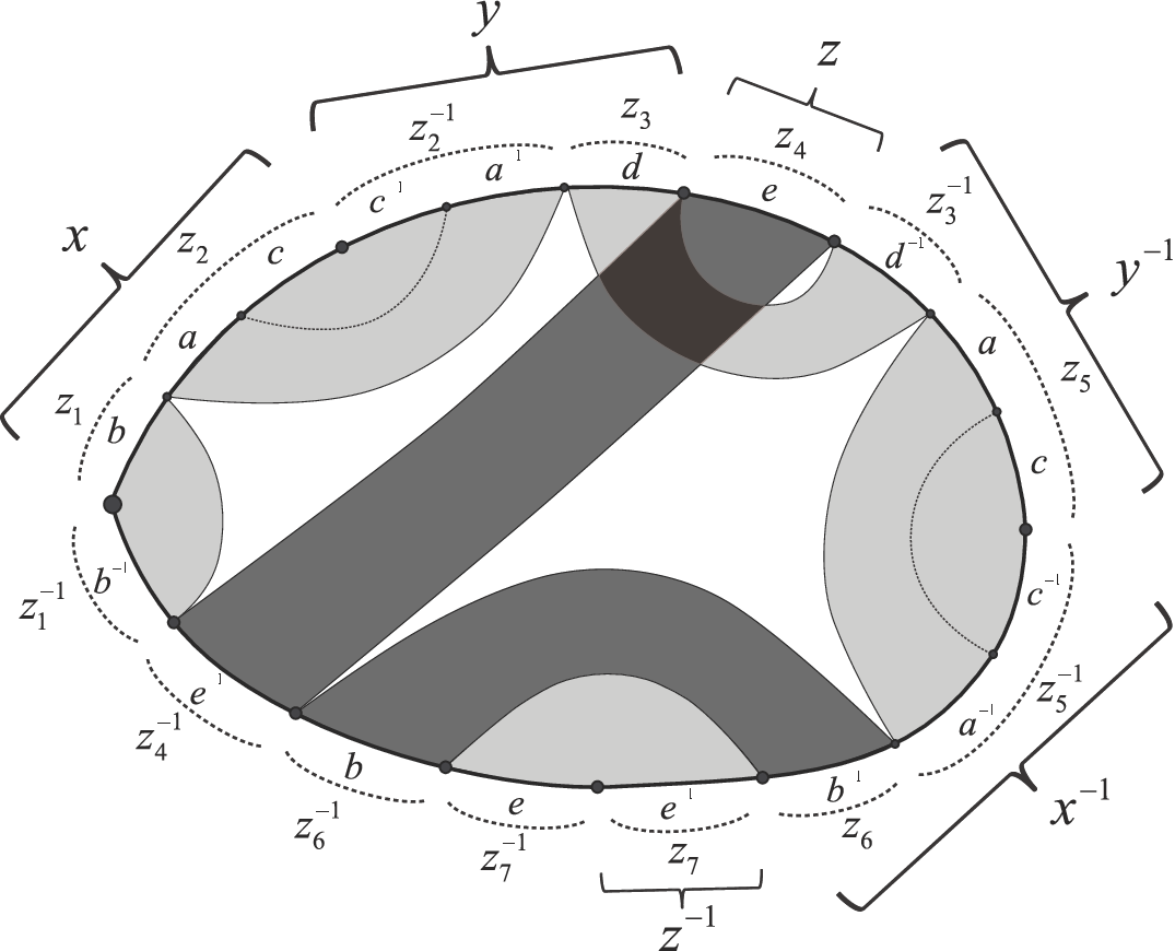
Content of Section 3.2.1
Write the equation in the form , see Equation (3).
By the cancellation scheme shown on Figure 3, we construct a partition table . To every end of a band on Figure 3, we associate a variable or its inverse . We can write the variables as words in the variables ’s. Two variables and commute if and only if the corresponding bands cross. Thus, the partition table associated to the equation and its solution , , is given below
In the above notation, it is easy to see that every variable , occurs in the words precisely once, and that .
Content of Section 3.2.2
We now construct the generalised equation associated to the partition table . Consider the word in the free monoid :
The variables of the generalised equation are (equivalently, the set of boundaries of the combinatorial generalised equation is ).
For every pair of distinct occurrences of in we construct a pair of dual variable bases and the corresponding basic equation. For example, and . We introduce a pair of dual bases , and so that
The corresponding basic equation is , see Figure 4. The following table describes all basic equations thus constructed.
| pair of occurrences | pair of dual bases | corresponding basic equation |
|---|---|---|
| , | ||
| , | ||
| , | ||
| , | ||
| , | ||
| , | ||
| , |
For every pair of distinct occurrences of (correspondingly, of , or of ) in , we construct a pair of dual variable bases and the corresponding basic equation. For example, , . We introduce a pair of dual bases , , where so that
The corresponding basic equation is , see Figure 4. The following table describes all basic equations thus constructed.
| pair of occurrences | pair of dual bases | corresponding basic equation |
|---|---|---|
| , | ||
| , | ||
| , |
Here , , .
For , we construct a constant base and a coefficient equation. For example, . We introduce a constant base so that
The corresponding coefficient equation is , see Figure 4. The following table describes all coefficient equations.
| an occurrence | constant base | corresponding coefficient equation |
|---|---|---|
The set of boundary connections of is empty. This defines the generalised equation shown on Figure 4.
The set of pairs such that in and consists of:
To define the relation we have to make sure that the set is symmetric and satisfies condition () of Definition 3.4. Since we have the equations , , we get that
Clearly, the relation has to be symmetric, but, in this section, we further write only one of the two symmetric pairs. This defines the constrained generalised equation .
We represent generalised equations graphically in the way shown on Figure 4.

Content of Section 3.3.1
By Corollary 3.22 for every pair there exists a pair such that the diagram given in Corollary 3.22 is commutative. We now construct the set that defines a generalised equation over . We construct the elements of the sets that correspond to the solution , , .
Recall that the partially commutative group is defined by the commutation graph shown on Figure 2. The definition of DM-normal form in the partially commutative monoid is given by induction on the number of thin clans. In our example thin clans of are , , , and .
Consider the DM-normal form in with respect to the thin clan . Note that for , we have that is not written in the DM-normal form. We introduce a new variable and write , (here the corresponding permutation on is trivial) and . Notice that is in the DM-normal form.
Below we describe all the elements for the solution , , .
Analogously, we describe all the elements for the solution , , .
For the tuple we construct the generalised equation . Equations corresponding to , are:
Equations that equate different decompositions of the same variable are obtained as follows:
This defines the generalised equation (by the definition, the set of boundary connections of is empty).
Set
- •
, , if ;
- •
if for some ;
- •
if for some ;
We define to be the minimal subset of that is symmetric and satisfies condition () of Definition 3.4.
Remark 3.23.
Observe, that the initial system of equations contains a single equation in three variables. The generalised equation is a system of equations in variables. The generalised equation is a system of equations in at least variables. (Note that for , we constructed the system of equations over the monoid . We still should have constructed a combinatorial generalised equation associated to this system, see Lemma 3.3.)
Notice that, the above considered example describes only one generalised equation (which was traced by a particular solution of ). Consideration of all the finite collection of the generalised equations corresponding to the “simple” system of equations , can only be done on a computer.
This picture is, in fact, general. The size of the systems grows dramatically and makes difficult to work with examples.
4. The process: construction of the tree
“Es werden aber bei uns in der Regel keine aussichtslosen Prozesse geführt.”
Franz Kafka, “Der Prozess”
In the previous section we reduced the study of the set of solutions of a system of equations over a partially commutative group to the study of solutions of constrained generalised equations over a free monoid. In order to describe the solutions of constrained generalised equations over a free monoid, in this section we describe a branching rewriting process for constrained generalised equations.
In his important papers [Mak77] and [Mak82], G. Makanin devised a process for proving that the compatibility problem of systems of equations over a free monoid (over a free group) is decidable. This process was later developed by A. Razborov. In his work [Raz85], [Raz87], gave a complete description of all solutions of a system of equations. A further step was made by O. Kharlampovich and A. Miasnikov. In [KhM05a], in particular, the authors extend Razborov’s result to systems of equations with parameters. In [KhM05b] the authors establish a correspondence between the process and the JSJ decomposition of fully residually free groups.
In another direction, Makanin’s result (on decidability of equations over a free monoid) was developed by K.Schulz, see [Sch90], who proved that the compatibility problem of equations with regular constraints over a free monoid is decidable.
It turns out to be that the compatibility problem of equations over numerous groups and monoids can be reduced to the compatibility problem of equations over a free monoid with constraints. This technique turned out to be rather fruitful. G. Makanin was the first to do such a reduction. In [Mak82], in particular, he reduced the compatibility problem of equations over a free group to the decidability of the compatibility problem for free monoids. Later V. Diekert, C. Gutiérrez and C. Hagenah, see [DGH01], reduced the compatibility problem of systems of equations over a free group with rational constraints to compatibility problem of equations with regular constraints over a free monoid.
The reduction of compatibility problem for hyperbolic groups to free group was made in [RS95] by E. Rips and Z. Sela; for relatively hyperbolic groups with virtually abelian parabolic subgroups in [Dahm05] by F. Dahmani, for HNN-extensions with finite associated subgroups and for amalgamated products with finite amalgamated subgroups in [LS08] by M. Lohrey and G. Sénizergues, for partially commutative monoids in [Mat97] by Yu. Matiasevich, for partially commutative groups in [DM06] by V. Diekert and A. Muscholl, for graph product of groups in [DL04] by V. Diekert and M. Lohrey.
The complexity of Makanin’s algorithm has received a great deal of attention. The best result about arbitrary systems of equations over monoids is due to W. Plandowski. In a series of two papers [Pl99a, Pl99b] he gave a new approach to the compatibility problem of systems of equations over a free monoid and showed that this problem is in PSPACE. An important ingredient of Plandowski’s method is data compression in terms of exponential expressions. This approach was further extended by Diekert, Gutiérrez and Hagenah, see [DGH01] to systems of equations over free groups. Recently, O. Kharlampovich, I. Lysënok, A. Myasnikov and N. Touikan have shown that solving quadratic equations over free groups is NP-complete, [KhLMT08].
Another important development of the ideas of Makanin is due to E. Rips and is now known as the Rips’ machine. In his work Rips interprets Makanin’s algorithm in terms of partial isometries of real intervals, which leads him to a classification theorem of finitely generated groups that act freely on -trees. A complete proof of Rips’ theorem was given by D. Gaboriau, G. Levitt, and F. Paulin, see [GLP94], and, independently, by M. Bestvina and M. Feighn, see [BF95], who also generalised Rips’ result to give a classification theorem of groups that have a stable action on -trees.
The process we describe is a rewriting system based on the “divide and conquer” algorithm design paradigm (more precisely, “divide and marriage before conquest” technique, [Bl99]).
For a given generalised equation , this branching process results in a locally finite and possibly infinite oriented rooted at tree , . The vertices of the tree are labelled by (constrained) generalised equations over . The edges of the tree are labelled by epimorphisms of the corresponding coordinate groups. Moreover, for every solution of , there exists a path in the tree from the root vertex to a vertex and a solution of such that the solution is a composition of the epimorphisms corresponding to the edges in the tree and the solution . Conversely, every path from the root to a vertex in and any solution of give rise to a solution of , see Proposition 4.13.
The tree is constructed by induction on the height. Let be a vertex of height . One can check under the assumptions of which of the 15 cases described in Section 4.4 the generalised equation falls. If falls under the assumptions of Case 1 or Case 2, then is a leaf of the tree . Otherwise, using the combination of elementary and derived transformations (defined in Sections 4.2 and 4.3) given in the description of the corresponding (to ) case, one constructs finitely many generalised equations and epimorphisms from the coordinate group of to the coordinate groups of the generalised equations constructed.
We finish this section (see Lemma 4.19) by proving that infinite branches of the tree , as in the case of free groups, correspond to one of the following three cases:
- (A)
Case 7-10: Linear case (Levitt type, thin type);
- (B)
Case 12: Quadratic case (surface type, interval exchange type);
- (C)
Case 15: General case (toral type, axial type).
4.1. Preliminary definitions
In this section we give some definitions that we use throughout the text.
Definition 4.1.
Let be a generalised equation. We partition the set of all closed sections of into a disjoint union of two subsets
The sections from and , are called correspondingly, variable, and constant sections.
To organise the process properly, we partition the closed sections of in another way into a disjoint union of two sets, which we refer to as parts:
Sections from are called active, and sections from are called non-active. We set
If not stated otherwise, we assume that all sections from belong to the active part .
If , then every item (or base) from is called active or non-active, depending on the type of .
Definition 4.2.
We say that a generalised equation is in the standard form if the following conditions hold.
- (1)
All non-active sections are located to the right of all active sections. Formally, there are numbers such that and are, correspondingly, unions of all active and all non-active sections.
- (2)
All constant bases belong to , and for every letter there is at most one constant base in labelled by .
- (3)
Every free variable of belongs to a section from .
We will show in Lemma 4.12 that every generalised equation can be taken to the standard form.
4.2. Elementary transformations
In this section we describe elementary transformations of generalised equations. Recall that we consider only formally consistent generalised equations. In general, an elementary transformation associates to a generalised equation a finite set of generalised equations , and a collection of surjective homomorphisms such that for every pair there exists a unique pair such that the following diagram commutes.
Since the pair is defined uniquely, we have a well-defined map .
Every elementary transformation is first described formally and then we give an example using graphic representations of generalised equations, the latter being much more intuitive. It is a good exercise to understand what how the elementary transformations change the system of equations corresponding to the generalised equation.
: Cutting a base
Suppose that contains a boundary connection .
The transformation carries into a single generalised equation which is obtained from as follows. To obtain from we
- •
replace (cut in ) the base by two new bases and , and
- •
replace (cut in ) by two new bases and ,
so that the following conditions hold.
If , then
If , then
Put
Let be a boundary connection in . If , then we replace by . If , then we replace by . Notice that from property (2) of Definition 3.9, it follows that (or ) is a boundary connection in the new generalised equation.
We define the new generalised equation , by setting . The resulting generalised equation is also formally consistent. Put , see Figure 5.

: Transferring a base
Let a base of a generalised equation be contained in the base , i.e., . Suppose that the boundaries and are -tied, i.e. there are boundary connections of the form and . Suppose also that every -tied boundary is -tied.
The transformation carries into a single generalised equation which is obtained from as follows. To obtain from we transfer from the base to the base and adjust all the basic and boundary equations (see Figure 6). Formally, we replace by a new base such that and replace each -boundary connection with a new one where and are related by a -boundary connection .
By definition, set . We therefore defined a generalised equation , set .

: Removing a pair of matched bases
Let and be a pair of matched bases in . Since is formally consistent, one has , and every -boundary connection is of the form .
The transformation applied to results in a single generalised equation which is obtained from by removing the pair of bases with all the -boundary connections and setting , see Figure 7.

Remark 4.3.
Observe that for , the set consists of a single generalised equation , such that and have the same set of variables and . The identity isomorphism , where is the free group on , trivially induces a -isomorphism from to and an -isomorphism from to .
Moreover, if is a solution of , then the tuple is a solution of , since the substitution of into the equations of result in graphical equalities.
: Removing a linear base
Suppose that in a variable base does not intersect any other variable base, i.e. the items are contained only in one variable base . Moreover, suppose that all boundaries that intersect are -tied, i.e. for every , there exists a boundary such that is a boundary connection in . Since is formally consistent, we have and if , and and if .
The transformation carries into a single generalised equation which is obtained from by deleting the pair of bases and ; deleting all the boundaries , deleting all -boundary connections, re-enumerating the remaining boundaries and setting .
We define the epimorphism , where is the free group on and is the set of variables of , as follows:
It is not hard to see that induces a -isomorphism and an -isomorphism from to . Furthermore, if is a solution of the tuple (obtained from in the same way as is obtained from ) is a solution of .

Remark 4.4.
Every time when we transport or delete a closed section (see , , , ), we re-enumerate the boundaries as follows.
The re-enumeration of the boundaries is defined by the correspondence , :
Naturally, in this case we write meaning that
: Introducing a new boundary
Suppose that a boundary intersects a base and is not -tied.
The transformation -ties the boundary in all possible ways, producing finitely many different generalised equations. To this end, let be a boundary intersecting . Then we perform one of the following two transformations (see Figure 9):

- (1)
Introduce the boundary connection in , provided that the resulting generalised equation is formally consistent. Define the set to be the minimal subset that contains , is symmetric and satisfies condition (), see Definition 3.4. This defines the generalised equation .
The identity isomorphism , where is the free group on , trivially induces a -epimorphism from to and an -epimorphism from to .
Observe that is not necessarily an isomorphism. More precisely, is not an isomorphism whenever the boundary equation corresponding to the boundary connection does not belong to . In this case is a proper epimorphism. Moreover, if is a solution of , then the tuple is a solution of .
- (2)
Introduce a new boundary between and ; introduce a new boundary connection in . Denote the resulting generalised equation by . Set (below we assume that the boundaries of are labelled ):
We then make the set symmetric and complete it in such a way that it satisfies condition (), see Definition 3.4. This defines the generalised equation .
We define the -monomorphism , where is the free group on and is the set of variables of , as follows:
Observe that the -monomorphism induces a -isomorphism and an -isomorphism from to . Moreover, if is a solution of , then the tuple (obtained from in the same way as is obtained from ) is a solution of .
Lemma 4.5.
Let be a generalised equation obtained from by an elementary transformation and let be the corresponding epimorphism. There exists an algorithm which determines whether or not the epimorphism is a proper epimorphism.
Proof.
The only non-trivial case is when and no new boundaries were introduced. In this case is obtained from by adding a new boundary equation , which is effectively determined by and . In this event, the coordinate group
is a quotient of the group . The homomorphism is an isomorphism if and only if , or, equivalently, . The latter condition holds if and only if vanishes on all solutions of the system of equations in , i.e. if the following universal formula (quasi identity) holds in :
This can be verified effectively, since the universal theory of is decidable, see [DL04]. ∎
Lemma 4.6.
Let be a generalised equation obtained from by an elementary transformation and let be the corresponding epimorphism. Then there exists a homomorphism
such that induces an epimorphism
and the epimorphism . In other words, the following diagram commutes:
Proof.
Follows by examining the definition of for every elementary transformation . ∎
4.3. Derived transformations
In this section we describe several useful transformations of generalised equations. Some of them are finite sequences of elementary transformations, others result in equivalent generalised equations but cannot be presented as a composition of finitely many elementary transformations.
In general, a derived transformation associates to a generalised equation a finite set of generalised equations , and a collection of surjective homomorphisms such that for every pair there exists a unique pair such that the following diagram commutes.
Since the pair is defined uniquely, we have a well-defined map .
Closing a section
Let be a section of . The transformation makes the section closed. To perform , using , we -tie the boundary (the boundary ) in every base containing (, respectively). Using , we cut all the bases containing (or ) in the boundary (or in ), see Figure 10.

Transporting a closed section
Let be a closed section of a generalised equation . The derived transformation takes to a single generalised equation obtained from by cutting out from the interval together with all the bases, and boundary connections on and moving to the end of the interval or between two consecutive closed sections of , see Figure 11. Then we re-enumerate all the items and boundaries of the generalised equation obtained as appropriate, see Remark 4.4. Clearly, the original equation and the new one have the same solution sets and their coordinate groups are isomorphic (the isomorphism is induced by a permutation of the variables ).

Completing a cut
Let be constrained a generalised equation. The derived transformation carries into a single generalised equation by applying to all boundary connections in . Formally, for every boundary connection in we cut the base in applying . Clearly, the generalised equation does not depend on the choice of a sequence of transformations . Since, by Remark 4.3, induces the identity isomorphism between the coordinate groups, equations and have isomorphic coordinate groups and the isomorphism is induced by the identity map .
Kernel of a generalised equation
The derived transformation applied to a generalised equation results in a single generalised equation constructed below.
Applying , if necessary, one can assume that a generalised equation does not contain boundary connections. An active base is called eliminable if at least one of the following holds:
- a)
contains an item with ;
- b)
at least one of the boundaries is different from and it does not touch any other base (except ).
An elimination process for consists of consecutive removals (eliminations) of eliminable bases until there are no eliminable bases left in the generalised equation. The resulting generalised equation is called the kernel of and we denote it by . It is easy to see that does not depend on the choice of the elimination process. Indeed, if has two different eliminable bases , , and elimination of results in a generalised equation then by induction on the number of eliminations is defined uniquely for . Obviously, is still eliminable in , as well as is eliminable in . Now eliminating and from and respectively, we get the same generalised equation . By induction hence the result.
We say that a variable belongs to the kernel, if either belongs to at least one base in the kernel, or is constant.
For a generalised equation we denote by the generalised equation which is obtained from by deleting all free variables in and setting to be the restriction of to the set of variables in . Obviously,
where is the set of free variables in and is a variable of (in particular, may be one of the free variables ).
Let us consider what happens in the elimination process on the level of coordinate groups.
We start with the case when just one base is eliminated. Let be an eliminable base in . Denote by the generalised equation obtained from by eliminating and let , where .
- (1)
Suppose and , i.e. falls under the assumption a) of the definition of an eliminable base. Then the variable occurs only once in (in the equation corresponding to the base , denote this equation by ). Therefore, in the coordinate group the relation can be written as , where does not contain . Consider the generalised equation obtained from by deleting the equation and the item . The presentation of the coordinate group of is obtained from the presentation of the coordinate group of using a sequence of Tietze transformations, thus these groups are isomorphic. We define the relation as the restriction of to the set , and .
It follows that
We therefore get that
and
(5) where are the free variables of distinct from . Note that all the groups and equations which occur above can be found effectively.
- (2)
Suppose now that falls under the assumptions of case b) of the definition of an eliminable base, with respect to a boundary . Then in all the equations of the generalised equation but , the variable occurs as a part of the subword . In the equation the variable either occurs once or it occurs precisely twice and in this event the second occurrence of (in ) is a part of the subword . It is obvious that the tuple
forms a basis of the ambient free group generated by . We further assume that is a system of equations in these variables. Notice, that in the new basis, the variable occurs only once in the generalised equation , in the equation . Hence, as in case (1), the relation can be written as , where does not contain .
Therefore, if we eliminate the relation , then the set is a generating set of . In the coordinate group the commutativity relations rewrite as follows:
This shows that
where is the generalised equation obtained from by deleting the boundary and is the restriction of to the set . Denote by the generalised equation obtained from by adding a free variable . It now follows that
(6) where are the free variables of distinct from . Notice that all the groups and equations which occur above can be found effectively.
By induction on the number of steps in the elimination process we obtain the following lemma.
Lemma 4.7.
In the above notation,
where is a set of free variables of , and is a certain computable set of commutators of words in .
Proof.
Let
where is obtained from by eliminating an eliminable base, . It is easy to see (by induction on ) that for every
Moreover, if is obtained from as in case (2) above, then (in the above notation)
The statement of the lemma now follows from the remarks above and Equations (5) and (6). Note that the cardinality of the set is the number of free variables of minus . ∎
Entire transformation
In order to define the derived transformation we need to introduce several notions. A base of the generalised equation is called a leading base if . A leading base is called a carrier if for any other leading base we have . Let be a carrier base of . Any active base with is called a transfer base (with respect to ).
Suppose now that is a generalised equation with for each in the active part of . The entire transformation is the following sequence of elementary transformations.
We fix a carrier base of . For any transfer base we -tie (applying ) all boundaries that intersect . Using we transfer all transfer bases from onto . Now, there exists some such that belong to only one base while belongs to at least two bases. Applying we cut in the boundary . Finally, applying , we delete the section , see Figure 16.
Let be the boundary between the active and non-active parts of , i.e. is the active part of and is the non-active part of .
Definition 4.8.
For a pair , we introduce the following notation
| (7) |
| (8) |
where is the set of all variable bases for which either or belongs to the active part of .
We call the number the excess of the solution of the generalised equation .
Every item of the section belongs to at least two bases, each of these bases belongs to , hence .
Notice, that if for every item of the section one has , for every solution of the excess . Informally, in some sense, the excess of measures how far the generalised equation is from being quadratic (every item in the active part is covered twice).
Lemma 4.9.
Let be a generalised equation such that every item from the active part of is covered at least twice. Suppose that and the carrier base of and its dual belong to the active part of . Then the excess of the solution equals the excess of the solution , i.e. .
Proof.
By the definition of the entire transformation , it follows that the word is a terminal subword of the word , i.e.
On the other hand, since , the non-active parts of and coincide. Therefore, is the terminal subword of the word , i.e. the following graphical equality holds:
So we have
| (9) |
where, in the above notation, if (and thus has been completely eliminated in ), then ; otherwise, .
Identifying closed constant sections
Let and be two constant bases in with labels and , where and , . Suppose that the sections and are closed.
The transformation applied to results in a single generalised equation which is obtained from in the following way, see Figure 12. Introduce a new variable base with its dual such that
Then we transfer all bases from onto using , remove the bases and , remove the item , re-enumerate the remaining items and adjust the relation as appropriate, see Remark 4.4.
The corresponding homomorphism is induced by the composition of the homomorphisms defined by the respective elementary transformations. Obviously, is an isomorphism.
Lemma 4.10.
Let be a generalised equation and be a solution of so that
Then one has . Furthermore, in the case that or this inequality is strict .
Proof.
Proof is by straightforward examination of descriptions of elementary and derived transformations. ∎
Lemma 4.11.
Let be a generalised equation obtained from by a derived transformation and let be the corresponding epimorphism. Then there exists a homomorphism
such that induces an epimorphism
and the epimorphism . In other words, the following diagram commutes:
Proof.
Follows by examining the definition of for every derived transformation and Lemma 4.6. ∎
Lemma 4.12.
Using derived transformations, every generalised equation can be taken to the standard form.
Let be obtained from by an elementary or a derived transformation and let be in the standard form. Then is in the standard form.
Proof.
Proof is straightforward. ∎
4.4. Construction of the tree
In this section we describe a branching process for rewriting a generalised equation . This process results in a locally finite and possibly infinite tree . In the end of the section we describe infinite paths in . We summarise the results of this section in the proposition below.
Proposition 4.13.
For a (constrained) generalised equation over , one can effectively construct a locally finite, possibly infinite, oriented rooted at tree , , such that:
- (1)
The vertices of are labelled by generalised equations over .
- (2)
The edges of are labelled by epimorphisms
The edges , where is a leaf of and , are labelled by proper epimorphisms. All the other epimorphisms are isomorphisms, in particular, edges that belong to infinite branches of the tree are labelled by isomorphisms.
- (3)
Given a solution of , there exists a path and a solution of such that
Conversely, for every path in and every solution of the homomorphism
gives rise to a solution of .
Definition 4.14.
Denote by the number of bases in the active sections of and by the number of open boundaries in the active sections.
For a closed section denote by the number of bases in . The complexity of a generalised equation is defined as follows
Remark 4.15.
We use the following convention. Let be a generalised equation. By a function of a generalised equation we mean a function of the parameters , , and .
We begin with a general description of the tree and then construct it using induction on its height. For each vertex in there exists a generalised equation associated to . Recall, that we consider only formally consistent generalised equations. The initial generalised equation is associated to the root , . For each edge there exists a unique surjective homomorphism associated to .
If
is a path in , then by we denote the composition of corresponding homomorphisms
We call this epimorphism the canonical homomorphism from to
There are two kinds of edges in : principal and auxiliary. Every edge constructed is principal, if not stated otherwise. Let be an edge of , we assume that active (non-active) sections in are naturally inherited from . If is a principal edge, then there exists a finite sequence of elementary and derived transformations from to and the homomorphism is a composition of the homomorphisms corresponding to these transformations.
Since both elementary and derived transformations uniquely associate a pair to :
a solution of defines a path in the tree . We call such a path the path defined by a solution in .
Let be a generalised equation. We construct an oriented rooted tree . We start from the root and proceed by induction on the height of the tree.
Suppose, by induction, that the tree is constructed up to height , and let be a vertex of height . We now describe how to extend the tree from . The construction of the outgoing edges from depends on which of the case described below takes place at the vertex . We always assume that:
If the generalised equation satisfies the assumptions of Case , then does not satisfy the assumptions of all the Cases , with .
The general guideline of the process is to use the entire transformation to transfer bases to the right of the interval. Before applying the entire transformation one has to make sure that the generalised equation is “clean”. The stratification of the process into 15 cases, though seemingly unnecessary, is convenient in the proofs since each of the cases has a different behaviour with respect to “complexity” of the generalised equation, see Lemma 4.18.
Preprocessing
In we transport closed sections using in such a way that all active sections are at the left end of the interval (the active part of the generalised equation), then come all non-active sections.
Termination conditions: Cases 1 and 2
Case 1: The homomorphism is not an isomorphism, or, equivalently, the canonical homomorphism , where is an edge of , is not an isomorphism.
The vertex , in this case, is a leaf of the tree . There are no outgoing edges from .
Case 2: The generalised equation does not contain active sections.
Then the vertex is a leaf of the tree . There are no outgoing edges from .
Moving constant bases to the non-active part: Cases 3 and 4
Case 3: The generalised equation contains a constant base in an active section such that the section is not closed.
In this case, we make the section closed using the derived transformation .
Case 4: The generalised equation contains a constant base such that the section is closed.
In this case, we transport the section to using the derived transformation . Suppose that the base is labelled by a letter . Then we identify all closed sections of the type , which contain a constant base with the label , with the transported section , using the derived transformation . In the resulting generalised equation the section becomes a constant section, and the corresponding edge is auxiliary, see Figure 12 (note that produces a finite set of generalised equations, Figure 12 shows only one of them).

Moving free variables to the non-active part: Cases 5 and 6
Case 5: The generalised equation contains a free variable in an active section.
Using , we transport the section to the very end of the interval behind all the items of . In the resulting generalised equation the transported section becomes a constant section, and the corresponding edge is auxiliary.
Case 6: The generalised equation contains a pair of matched bases in an active section.
In this case, we perform and delete it, see Figure 13.

Remark 4.16.
If does not satisfy the conditions of any of the Cases 1-6, then the generalised equation is in the standard form.
Eliminating linear variables: Cases 7-10
Case 7: There exists an item in an active section of such that and such that both boundaries and are closed.
Then, we remove the closed section together with the linear base using .
Case 8: There exists an item in an active section of such that and such that one of the boundaries , is open, say , and the other is closed.
In this case, we first perform and -tie by the only base it intersects; then using we cut in ; and then we delete the closed section using , see Figure 14.

Case 9: There exists an item in an active section of such that and such that both boundaries and are open. In addition, there is a closed section such that contains exactly two bases and , and is not a pair of matched bases, i.e. ; moreover, in the generalised equation all the bases obtained from by when constructing from , do not belong to the kernel of .
In this case, using we -tie all the boundaries that intersect ; using , we transfer onto ; and remove together with the closed section using , see Figure 15.
Case 10: There exists an item in an active section of such that and such that both boundaries and are open.
In this event we close the section using and remove it using , see Figure 15.

Tying a free boundary: Case 11
Case 11: Some boundary in the active part of is free.
Since the assumptions of Case 5 are not satisfied, the boundary intersects at least one base, say, .
In this case, we -tie using .
Quadratic case: Case 12
Case 12: For every item in the active part of we have .
We apply the entire transformation , see Figure 16.

Removing a closed section: Case 13
Case 13: For every item in the active part of we have , and for at least one item in the active part. Moreover, for some active base the section is closed.
In this case, using , we transport the section to the beginning of the interval (this makes a carrier base). We then apply the entire transformation (note that in this case the whole section is removed).
Tying a boundary: Case 14
Case 14: For every item in the active part of we have , and for at least one item in the active part. Moreover, some boundary in the active part touches some base , intersects some base , and is not -tied.
In this case, using , we -tie .
General case: Case 15
Case 15: For every item in the active part of we have , and for at least one item in the active part. Moreover, every active section is not closed and every boundary is -tied in every base it intersects.
We first apply the entire transformation . Then, using , we -tie every boundary in the active part that intersects a base and touches at least one base. This results in finitely many new vertices connected to by principal edges.
If, in addition, satisfies the assumptions of Case 15.1 below, then besides the principal edges already constructed, we construct a few more auxiliary edges outgoing from the vertex .
Case 15.1: The carrier base of the generalised equation intersects with its dual .
We first construct an auxiliary generalised equation (which does not appear in the tree ) as follows. Firstly, we add a new constant section to the right of all the sections in (in particular, is a new free variable). Secondly, we introduce a new pair of dual variable bases so that
Notice that can be obtained from if we apply to and delete the base together with the closed section . Let
be the isomorphism induced by . The assumptions of Case 15 still hold for . Note that the carrier base of is the base . Applying the transformations described in Case 15 to (first and then ), we obtain a set of new generalised equations and the set of corresponding epimorphisms of the form:
Now for each generalised equation we add a vertex and an auxiliary edge in the tree . The edge is labelled by the homomorphism which is the composition of homomorphisms and , . We associate the generalised equation to the vertex .
The tree is therefore constructed. Observe that, in general, is an infinite locally finite tree.
If the generalised equation satisfies the assumptions of Case , then we say that the vertex has type and write .
Lemma 4.17.
For any vertex of the tree there exists an algorithm to decide whether or not is of type , .
Proof.
The statement of the lemma is obvious for all cases, except for Case 1.
To decide whether or not the vertex is of type 1 it suffices to show that there exists an algorithm to check whether or not the canonical epimorphism associated to an edge in is a proper epimorphism. This can be done effectively by Lemma 4.5. ∎
Lemma 4.18 (cf. Lemma 3.1, [Raz87]).
Let be a principal edge of the tree . Then the following statements hold.
- (1)
If , then , moreover if , then this inequality is strict;
- (2)
If , then ;
- (3)
If and , then ;
- (4)
If , then .
Proof.
Straightforward verification. ∎
The following lemma gives a description of the infinite branches in the tree .
Lemma 4.19 (cf. Lemma 3.2, [Raz87]).
Let
| (10) |
be an infinite path in the tree . Then there exists a natural number such that all the edges of this path with are principal edges, and one of the following conditions holds:
Proof.
Firstly, note that Cases 1 and 2 can only occur once in the path (10).
Secondly, note Cases 3 and 4 can occur only finitely many times in the path (10), namely, at most times where is the number of constant bases in the original generalised equation . Therefore, there exists a natural number such that for all .
Now we show that the number of vertices () for which is bounded above by the minimal number of generators of the group , in particular, it cannot be greater than , where . Indeed, if a path from the root to a vertex contains vertices of type 5, then has at least free variables in the non-active part. This implies that the coordinate group has the free group of rank as a free factor, hence it cannot be generated by less than elements. Since is a surjective homomorphism, the group cannot be generated by less then elements. This shows that . It follows that there exists a number such that for every .
Since the path (10) is infinite, by Lemma 4.18, we may assume that for every one has , i.e. the complexity stabilises.
If is an auxiliary edge, where , then and satisfies the assumption of Case 15.1. In the notation of Case 15.1, we analyse the complexity of the generalised equation obtained from . As both bases and are transferred from the carrier base of to the non-active part, so the complexity decreases by at least two, i.e. . Observe also that . Hence , which derives a contradiction. Hence, if the edge is principal.
Suppose that . If , then the closed section containing the matched bases , does not contain any other bases (otherwise ). But then deriving a contradiction. We therefore get that for all one has .
If , then it is easy to see that or . Therefore, if we get that for every and we have case (B) of the lemma.
Suppose that for all .
Notice that the only elementary (derived) transformation that may produce free boundaries is and that is applied only in Case 6. Since for we have , we see that there are no new free boundaries in the generalised equations for . It follows that there exists a number such that for every .
Suppose now that for some , . It is easy to see from the description of Cases 13, 14 and 15 that . Since , this implies that for every . Then, by Lemma 4.18, we have that , for every . Furthermore, if , then . Hence there exists a number such that for all .
Suppose that . Note that there can be at most vertices of type 14 in a row starting at the vertex , hence there exists such that . From the description of Case 15 it follows that , thus , and we have case (C) of the lemma.
Finally, we are left with the case when for all the vertices of the path. We then have case (A) of the lemma. ∎
Remark 4.20.
5. Minimal solutions
In this section we introduce a reflexive, transitive relation on the set of solutions of a generalised equation. We use this relation to introduce the notion of a minimal solution with respect to a group of automorphisms of the coordinate group of the generalised equation. In the end of the section we describe the behaviour of minimal solutions with respect to the elementary transformations.
Let and be two geodesic words from . Consider the product of and . The geodesic of the element can be written as follows , where , and is the greatest (left) common divisor of and (in the sense of [EKR05]). Notice that if the word is not geodesic, then it follows that is non-trivial. We call the cancellation divisor of and and we denote it by .
Definition 5.1.
Let be a partially commutative -group, let be a generalised equation with coefficients from over the free monoid . Let be an arbitrary group of -automorphisms of . For solutions and of the generalised equation we write if there exists a -endomorphism of the group and an automorphism such that the following conditions hold:
- (1)
;
- (2)
for any , , if the word , , is geodesic as written, then the word is geodesic as written;
- (3)
for any , such that the word , , is not geodesic, if
(11) for some , then either the word is geodesic as written or
(12) where .
Obviously, the relation ‘’ is transitive. We would like to draw the reader’s attention to the fact that the relation does not imply relations on the lengths of the solutions and .
The motivation for property (3) in the above definition is the following lemma.
Lemma 5.2.
Let be a partially commutative -group, let be a generalised equation with coefficients from over the free monoid . Let be an arbitrary group of -automorphisms of and let and be two solutions of the generalised equation such that . Then for any word such that the is geodesic as written (treated as an element of ), the word is geodesic as written (treated as an element of ).
Proof.
We use induction on the length of . If , then the statement follows, since by the definition of a solution of the generalised equation, the words and are both geodesic.
Let , , , be a word such that is geodesic and assume that is not geodesic. By induction hypothesis, the word is geodesic. Consider the cancellation divisor . Analogously, by induction hypothesis, the word is geodesic. Using the fact that the word is geodesic, we get that the cancellation divisor is, in fact, , and, in particular, no left divisor of the word left-divides . We thereby have that
- (a)
on one hand, the word is not geodesic and,
- (b)
on the other hand, by Proposition 3.18 of [EKR05], that .
Lemma 5.3.
Let the generalised equation be obtained from the generalised equation by one of the elementary transformation , i.e. for some . Let be a solution of and be a solution of so that the following diagram commutes
Let be another solution of so that , where is arbitrary. The -tuple of geodesic words of defined by the homomorphism is a solution of the generalised equation .
Proof.
Proof is by examination of the definitions of elementary transformations. We further use the notation introduced in the definitions of elementary transformations.
Suppose first that is obtained from by . Since, in this case, , we have that is a tuple of non-trivial geodesic words in . The elementary transformation is invariant on all the bases but the pair , . Therefore, we are left to prove that the words and are geodesic and that the equality is graphical.
Since is a geodesic word and , by Lemma 5.2 it follows that is geodesic. Similarly, is also geodesic. Since is a solution of , we have that
From the equalities
and the fact that the words and are geodesic, we obtain that the equality is graphical.
The other cases are similar and left to the reader. ∎
Definition 5.4.
Let be a generalised equation in variables and let be a solution of . Consider a matrix , constructed by the solution in the following way. The elements of the matrix are -vectors with entries from the set . We enumerate (in an arbitrary way) the set of all subsets of . Abusing the notation, in this definition if , then by we mean .
The vector has all of its components equal to if and only if the word is geodesic as written. The first component of the vector equals if and only if the word is not geodesic. The -th component of equals , , if for the -th set of Equation (11) is satisfied. Otherwise the -th component of equals .
We call the matrix , the cancellation matrix of the solution .
Definition 5.5.
A solution of is called minimal with respect to the group of automorphisms if there exist no solutions of the generalised equation so that and for all , and for at least one , .
Since the length of a solution is a positive integer, every strictly descending chain of solutions
is finite. It follows that for every solution of there exists a minimal solution such that .
Remark 5.6.
Note that given a solution , there exists a minimal solution (perhaps more than one) so that . Furthermore, there may exist minimal solutions and so that and . In this case one has for some and for some .
Remark 5.7.
Note that every generalised equation with coefficients from can be considered as a generalised equation with coefficients from for any partially commutative -group . Therefore, any solution of induces a solution of such that the following diagram commutes:
A solution of is minimal if so is any induced solution .
The reason for extending the generating set from to in the definition above, becomes clear in the proof of Lemma 6.19
Lemma 5.8.
Let the generalised equation be obtained from the generalised equation by one of the elementary transformation , i.e. for some and assume that is isomorphic to . Let be a solution of and be a solution of so that the following diagram commutes
If is a minimal solution of with respect to a group of automorphisms of , then is a minimal solution of with respect to the group of automorphisms .
Proof.
Assume the converse, i.e. is not minimal with respect to . Then there exists a solution of so that , for all and for some .
Let be a solution of the system of equations so that . By Lemma 5.3, is a solution of .
By Lemma 5.2, condition (2) from Definition 5.1 holds for the pair and . We now show that and derive a contradiction with the minimality of .
We now show that condition (3) from Definition 5.1 holds. Assume that for the pair , the word is not geodesic and that there exists a set such that Equation (12) fails, i.e. there exists a set and a letter such that and is a left divisor of . Without loss of generality, we further assume that . Write and as words in the ’s:
It follows that is a left divisor of for some and , and that
Therefore, Equation (12) fails for the solution and the set , where the set is a union of words that appear in the decomposition of a word and the set . Since , by condition (3) from Definition 5.1, Equation (11) fails for the solution and the corresponding set , i.e. there exists a letter such that and is a left divisor of .
Since , we get that is a left divisor of . Furthermore, since -commutes with the words ’s that appear in the decomposition of a word (where is the set corresponding to ), we get that . It follows that Equation (11) fails for the solution and the set . Hence, condition (3) from Definition 5.1 holds for the solutions and .
Furthermore, by condition (1) from Definition 5.1, we have , where , hence , and thus condition (1) from Definition 5.1 holds for the pair and . We thereby have proven that .
Finally, since , and for all and for some , we get that for all and for some , contradicting the minimality of . ∎
6. Periodic structures
Informally, the aim of this section is to prove the following strong version of the so-called Bulitko’s Lemma, [Bul70]:
Applying automorphisms from a finitely generated subgroup of the group of automorphisms of the coordinate group to a periodic solution either one can bound the exponent of periodicity of the solution (regular case, see Lemma 6.20), or one can get a solution of a proper equation (strongly singular case, see Lemma 6.17, and singular case, see Lemma 6.18).
Above, by a solution of a proper equation we mean a homomorphism from a proper quotient of the coordinate group of to .
This approach for free groups was introduced by A. Razborov. In [Raz85], he defines a combinatorial object, called a periodic structure on a generalised equation and constructs a finite set of generators for the group .
In Section 6.2 we give an example that follows the exposition of Section 6.1. We advise the reader unfamiliar with the definitions, to consult this example while reading Section 6.1.
6.1. Periodic structures
We fix till the end of this section a generalised equation in the standard form. Suppose that some boundary (between and ) in the active part of does not touch bases. Since the generalised equation is in the standard form, the boundary intersects at least one base . Using we -tie the boundary . Applying , if necessary, we may assume that the set of boundary connections in is empty and that each boundary of touches a base.
A cyclically reduced word in is called a period if is geodesic (in ) and is not a proper power treated as an element of the ambient free monoid. A word is called -periodic if is geodesic (treated as an element of ), and, is a subword of for some . Every -periodic word can be presented in the form
| (13) |
where is a cyclic permutation of , , and . The number is called the exponent of . A maximal exponent of a -periodic subword in a word is called the exponent of -periodicity of . We denote it by .
Definition 6.1.
Let be a generalised equation in the standard form. A solution of is called periodic with respect to a period , if for every closed variable section of one of the following conditions holds:
- (1)
is -periodic with exponent ;
- (2)
;
- (3)
is -periodic and ;
Moreover, condition (1) holds for at least one closed variable section of .
Let be a -periodic solution of . Then a section satisfying condition (1) of the above definition is called -periodic (with respect to ).
The following lemma gives an intuition about the kind of generalised equations that have periodic solutions.
Lemma 6.2.
Let be a generalised equation such that every closed section of is either constant or there exists a pair of dual bases , such that and intersect but do not form a pair of matched bases, and . Let be a solution of . Then there exists a period such that is -periodic.
Proof.
Consider a section . The boundary intersects the base , since the bases and overlap. We -tie the boundary , i.e. we introduce a boundary connection in such a way that is a solution of the generalised equation obtained. It follows that .
Repeating this argument, we obtain a finite set of boundaries , such that do and does not intersect , there is a boundary connection for all and induces a solution of the generalised equation obtained. This set of boundaries is finite, since the length of the solution is finite.
Let , , where and is a period. Then the section is -periodic. Indeed,
Using the boundary equations, we get that
thus , where .
Set , where . By definition, is -periodic. ∎
Below we introduce the notion of a periodic structure. The idea of considering periodic structures on is to subdivide the set of periodic solutions into subsets so that any two solutions from the same subset have the same set of “long items”, i.e. -periodic solutions that factor through the generalised equation and a periodic structure on satisfy the following property:
One can regard Lemma 6.5 below as a motivation for the definition of a periodic structure.
Definition 6.3.
Let be a generalised equation in the standard form without boundary connections. A periodic structure on is a pair , where
- (1)
is a non-empty set consisting of some variables , some variable bases , and some closed sections from such that the following conditions are satisfied:
- (a)
if and , then ;
- (b)
if , then ;
- (c)
if and , then ;
- (d)
there exists a function mapping the set of closed sections from into such that for every , the condition that and implies ;
- (a)
- (2)
is an equivalence relation on a certain set (defined in (e)) such that condition (f) is satisfied.
- (e)
Notice, that for every boundary belonging to a closed section in either there exists a unique closed section in containing , or there exist precisely two closed sections in containing . The set of boundaries of the first type we denote by , and of the second type by . Put
here are two “formal copies” of . We will use the following agreement: for any base if then by we mean and, similarly, if then by we mean .
- (f)
If then
- (e)
Remark 6.4.
For a given generalised equation , there exists only finitely many periodic structures on , and all of them can be constructed effectively. Indeed, every periodic structure is uniquely defined by the subset of items, bases and sections of that belong to and the relation .
Now we will show how to a -periodic solution of one can associate a periodic structure on . We define as follows. A closed section is in if and only if is -periodic. A variable is in if and only if for some and . A variable base is in if and only if either or contains an item from .
Put depending on whether in (13) the word is conjugate to or to .
Now let and . Then one can write in such a way that if , then the word is the terminal subword of the word , where is the infinite word obtained by concatenating the powers of , and is the initial subword of the word ; and if , then the word is the terminal subword of the word and is the initial subword of . By Lemma 1.2.9 [Ad75], the decomposition with these properties is unique; denote this decomposition by . We define the relation as follows:
Every periodic solution of induces a periodic structure on .
Lemma 6.5.
Let be a periodic solution of . Then is a periodic structure on .
Proof.
Let . Obviously, satisfies conditions (a) and (b) from Definition 6.3.
We now prove that satisfies condition (c) from Definition 6.3. Let and . There exists an item such that or . If , then, by construction, . If and , then , and hence, the word can be written in the form , where is a cyclic permutation of the word and . Since and from Definition 6.1, it follows that is an -periodic section, where . Then , where is a cyclic permutation of the word , , , and . From the equality and Lemma 1.2.9 [Ad75] it follows that is a cyclic permutation of the word . Consequently, is a cyclic permutation of the word . Therefore, is a -periodic section of with respect to , in other words, the length of is greater than or equal to and so .
If , and , then the equality = follows from the fact that given and , the word cannot be a cyclic permutation of the word , hence condition (d) of Definition 6.1 holds.
Since , from Lemma 1.2.9 in [Ad75] it follows that condition (f) also holds for the relation . ∎
Remark 6.6.
Now let us fix a non-empty periodic structure on a generalised equation . Item (d) of Definition 6.3 allows us to assume (after replacing the variables by on those closed sections for which ) that for all . Therefore, we may assume that for every item , the word is a subword of the word .
The rest of this section is devoted to defining the group of automorphisms . The idea is as follows. We change the set of generators of the coordinate group by and we use the new set of generators to give an explicit description of the generating set of the group of automorphisms .
To construct the set of generators of , the following definitions are in order. We refer the reader to Section 6.2 for an example.
Definition 6.7.
We construct the graph of a periodic structure . The set of vertices of the graph is the set of -equivalence classes. For a boundary , denote by the equivalence class of the relation to which it belongs. For each variable that belongs to a certain closed section from , we introduce an oriented edge from to , and an inverse edge . We label the edge by (correspondingly, ). For every path in the graph , we denote its label by , , .
The periodic structure is called connected, if its graph is connected.
Let be an arbitrary periodic structure of a generalised equation . Let be the connected components of the graph . The labels of edges of the component form (in the generalised equation ) a union of labels of closed sections from . Moreover, if a base belongs to a section from , then its dual , by condition (f) of Definition 6.3, also belongs to a section from . Define to be the union of the following three sets: the set of labels of edges from that belong to , closed sections to which these labels belong, and bases that belong to these sections. Define to be the restriction of the relation to . We thereby obtain a connected periodic structure whose graph is .
We further assume that the periodic structure is connected.
Let be the graph of a periodic structure and let be a path in , be its label, , . To simplify the notation we write instead of .
Lemma 6.8.
Let be a -periodic solution of a generalised equation , let be a periodic structure on and let be a cycle in the graph at the vertex , . Then there exists such that .
Proof.
If is an edge in the graph , and , are two decompositions corresponding to the boundaries from and respectively. Then, obviously, , . The statement follows if we multiply the values for all the edges in the cycle . ∎
Definition 6.9.
A generalised equation is called periodised with respect to a given periodic structure , if for every two cycles and based at the same vertex in the graph , there is a relation in . Note that, in particular in .
Let and .
Let be the subgraph of the graph having the same set of vertices as and the set of edges . Choose a maximal subforest in the graph and extend it to a maximal subforest of the graph . Since the periodic structure is connected by assumption, it follows that is a tree. Fix an arbitrary vertex of the graph and denote by the (unique) path in from to . For every edge not lying in , we introduce a cycle . Then the fundamental group is generated by the cycles (see, for example, the proof of Proposition III.2.1, [LS77]). This and the decidability of the universal theory of imply that the property of a generalised equation “to be periodised with respect to a given periodic structure” is algorithmically decidable. Indeed, it suffices to check if the following universal formula (quasi-identity) holds in (for every pair of cycles , ):
Furthermore, the set of elements
| (14) |
forms a basis of the free group generated by
If , then , by property (f) from Definition 6.3 and, consequently, the word is the label of a cycle from . Let . Then
| (15) |
where is the label of the path . Since , it follows that , where is a certain word in the indicated generators that can be constructed effectively (see Proposition III.2.1, [LS77]).
Let denote the image of the word in the abelianisation of . Denote by the free abelian group consisting of formal linear combinations , , and by its subgroup generated by the elements , and the elements , , .
By the classification theorem of finitely generated abelian groups, one can effectively construct a basis of such that
| (16) |
where is a basis of and is a basis of .
By Proposition I.4.4 in [LS77], one can effectively construct a basis , of the free (non-abelian) group such that , are the natural images of the elements , in .
Remark 6.10.
Notice that any equation in of the form
lifts to an equation in of the form
where is an element of the derived subgroup of . If the generalised equation is periodised, for any two cycles , we have that in . Hence, in .
Lemma 6.11.
Let be a periodised generalised equation. Then the basis can be chosen in such a way that for every either , where , , or for any solution we have .
Proof.
The set is a subset of the set of generators of contained in . Thus, this set can be extended to a basis of . Since, by (16), , for every there exists such that
It follows that the set which completes the set to a basis of , can be chosen so that the following equality holds:
Hence, by Remark 6.10, for any solution we have . Since is torsion-free, we have . ∎
Let be the set of edges of . Since is the spanning forest of the graph , it follows that ; in particular, .
Let be the free group generated by the variables of . Consider in the group a new set of generators defined below (we prove that the set is in fact a set of generators of in part (1) of Lemma 6.14).
Let be the origin of the edge . We introduce new variables
| (17) |
as follows
| (18) |
We denote by the union and by the union . Denote by the family of variables that do not belong to closed sections from . Let
Remark 6.12.
Note that without loss of generality we may assume that corresponds to the beginning of the period . Indeed, it follows from the definition of the periodic structure that for any cyclic permutation of , we have .
Lemma 6.13.
Let be a generalised equation periodised with respect to a periodic structure . Then for any cycle such that and for any solution of periodic with respect to a period , such that one has , where . In particular, one can choose a basis in such a way that for any one has , where .
Proof.
Let be a cycle such that the edges of are labelled by variables , . Observe that , where and are paths in the tree . Since , it follows that the origin and the terminus of the edge lie in the same connected component of the graph and, consequently, are connected by a path in the forest . Furthermore, and are paths in the tree connecting the same vertices; therefore, . Hence, , where is a certain cycle based at the vertex in the graph .
From the equality and by Lemma 6.8, we get that , where , , , . Hence and thus . From the construction of , it follows that the inequality holds for every item . Since the cycle is simple, we have that .
In particular, one has that for every , . By Lemma 6.11 one can choose a basis such that for every either and , or . ∎
The following lemma describes a generating set and the group of automorphisms of the coordinate group .
Lemma 6.14.
Let be a generalised equation periodised with respect to a periodic structure . Then the following statements hold.
- (1)
The system is equivalent to the union of the following two systems of equations:
and a system:
such that neither , , nor occurs in .
- (2)
If is a cycle based at the origin of , then the transformation which is identical on all the other elements from , extends to a -automorphism of .
- (3)
If and , , then the transformation defined by , which is identical on all the other elements from , extends to a -automorphism of .
Proof.
We first prove (1). It is easy to check that (in the above notation):
From Equation (14) and the discussion above it follows that
| (19) |
i.e. the sets and generate the same free group .
We now rewrite the equations from in terms of the new set of generators .
We first consider the relations induced by bases which do not belong to , i.e. basic equations of the form , where is a variable base, . By construction of the generating set , all the items which appear in these relations belong to the set
The elements of the sets and are generators in both basis. We now study how elements of rewrite in the new basis. Let , , . We have and
| (20) |
where is a path in and is a path in (see proof of Lemma 6.13). The variables , can occur in the right-hand side of Equation (20) (written in the basis ) only in and at most once. Moreover, the sign of this occurrence (if it exists) depends only on the orientation of the edge with respect to the root of the tree . If , then all the occurrences of the variable in the words written in the basis , with , are contained in the subwords of the form , i.e. in the subwords of the form , where is a certain cycle in the graph based at the origin of the edge . So the variable rewrites as a word in the generators , , .
Summarising, the basic equations corresponding to variable bases which do not belong to rewrite in the new basis as words in , , and .
In the new basis, the relations of the form , where , are, modulo commutators, words in , see Remark 6.10.
Since is periodised with respect to , we have
| (21) |
It follows that the system is equivalent to the union of the following two systems of equations in the new variables, a system
and a system (defined by the equations from ):
such that neither , , nor occurs in .
The transformations from statements (2) and (3) extend to an automorphism of . Indeed, by the universal property of the quotient, the following diagram commutes
It is easy to check that and that . Therefore, since by statement (1) of the lemma the system is equivalent to , we get that is an automorphism of . ∎
Definition 6.15.
Let be a generalised equation and let be a connected periodic structure on . We say that the generalised equation is strongly singular with respect to the periodic structure if one of the following conditions holds.
- (a)
The generalised equation is not periodised with respect to the periodic structure .
- (b)
We say that the generalised equation is singular with respect to the periodic structure if is not strongly singular with respect to the periodic structure and one of the following conditions holds
- (a)
The set has more than one element.
- (b)
The set has exactly one element, and (in the above notation) there exists a cycle , such that in .
Otherwise, we say that is regular with respect to the periodic structure . In particular if is singular or regular with respect to the periodic structure then is periodised.
When no confusion arises, instead of saying that is (strongly) singular (or regular) with respect to the periodic structure we say that the periodic structure is (strongly) singular (or regular).
Definition 6.16.
Let be a generalised equation and let be a periodic structure on . If is strongly singular with respect to , then we define the group of automorphisms of to be trivial.
Otherwise, i.e. if is singular or regular, we set to be the group of automorphisms of generated by the automorphisms induced by the automorphisms of described in statements (2) and (3) of Lemma 6.14. Note that by definition of singular and regular periodic structures, every such automorphism of induces an automorphism of and, therefore the group is finitely generated.
6.2. Example
In this section we give an example of a generalised equation , a periodic structure on the generalised equation and some of the constructions used in Section 6.1.
Let be a generalised equation shown on Figure 16 (the one to which the entire transformation is applied). Let be a periodic structure on defined as follows. Set . From part (a) of Definition 6.3 it follows that
From part (c) of Definition 6.3 we get that then . The set in part (e) of Definition 6.3 is defined to be . For the bases and their duals, we have
Therefore, there are three -equivalence classes: .
Suppose that is not strongly singular with respect to the periodic structure . Note that, using the decidability of the universal theory of , one could check if is strongly singular or not.
We construct the graph of the periodic structure as in Definition 6.7. The graph is shown on Figure 17. The edges of the graph are labelled by the corresponding items . In this example the set equals . We take the subgraph of whose edges are elements of and choose a maximal subtree of as shown on Figure 17. We extend the tree to a maximal subtree of , which is also shown on Figure 17.

We fix a vertex in . Then the fundamental group of with respect to is generated by the cycles :
Since, by definition, for any base one has that , the word labels a cycle in the graph . For the bases , we construct the corresponding cycles as in Equation (15):
Since the cycles belong to , these cycles can be written as words in the generators , as follows:
Let be the free abelian group generated by the images of the cycles , in the abelianisation of :
Consider the subgroup of generated by the images of and in the abelianisation of :
By the classification theorem of finitely generated abelian groups, there exist free abelian groups and such that and . To construct this decomposition (see Equation (16)), we construct a matrix with rows corresponding to the decomposition of the generators of in terms of the generators of and then apply the elementary transformations:
It follows that
The basis of and are and , respectively.
It is easy to see that the sets
form a base of and their images in are the sets and , correspondingly. Since , is singular with respect to the periodic structure .
Note that for every solution of we have . Indeed, since, by assumption, is periodised with respect to , the following equalities hold in the coordinate group :
The statement follows, since for any cycle , one has for any solution .
We construct the set of generators of used in Lemma 6.14. The set is a union of , (since ), , (since ), , and .
6.3. Strongly singular and singular cases
The next lemma states that if a generalised equation is strongly singular with respect to a periodic structure, then every periodic solution of is in fact a solution of a proper quotient, which can be effectively constructed. In other words, every periodic solution of the generalised equation can be obtained as a composition of a proper epimorphism and a solution of a proper generalised equation.
Lemma 6.17.
Let be a generalised equation without boundary connections, strongly singular with respect to the periodic structure . Then there exists a finite family of elements , so that for any solution of periodic with respect to a period , such that , one has that in for some and for all .
Proof.
Suppose that is strongly singular of type (a) with respect to . Since is not periodised with respect to there exist two cycles such that in . Then, by Lemma 6.8, for every -periodic solution of one has . In this case we set the family of elements to be the finite set of commutators of the form , where .
Suppose that is strongly singular of type (b) with respect to . Notice that by the universal property of the quotient, for every automorphism of the coordinate group , the following diagram commutes
where . Note that is an automorphism of if and only if . Since is strongly singular of type (b) with respect to , there exists an automorphism of described in statements (2) or (3) of Lemma 6.14 and a commutator such that , thus is non-trivial in . In this case, the finite set of elements of the form , where and is a generator of the group , satisfies the required properties.
Since the automorphism is identical on , , where , , , , and on , it follows that is identical on the set . Therefore, from and , we get that or . Without loss of generality, we may assume that .
By part (1) of Lemma 6.14, is a generating set of . The item can be written in the generators as a word . From the above discussion, it follows that .
Let be a solution of periodic with respect to a period such that . Since
| (22) |
by the definition of the automorphism , we get that
| (23) |
Therefore, .
The next lemma states that if a generalised equation is singular with respect to a periodic structure, then one can construct finitely many proper quotients of the coordinate group , such that for every periodic solution there exists an -automorphic image such that this image is in fact a solution of one of the quotients constructed. In other words, every solution of the generalised equation can be obtained as a composition of an automorphism from and a solution of a proper generalised equation.
Lemma 6.18.
Let be a generalised equation without boundary connections, singular with respect to the periodic structure . Then there exists a finite family of cycles in the graph such that the following conditions hold:
- (1)
, in ;
- (2)
for any solution of periodic with respect to a period , such that , there exists an -automorphic image of such that for some ;
- (3)
for any , ; and for any if , then , where , .
Proof.
Suppose that . Let be a solution of a generalised equation periodised with respect to the period such that . Let . By Lemma 6.8, , .
Without loss of generality we may assume that . Write , where either or . Applying the automorphism , , we get , hence the exponent of periodicity is reduced.
Applying the Euclidean algorithm, we get that there exists an automorphism from such that or . Set . Then the set satisfies conditions (1) and (2) of the lemma.
In the notation of Lemma 6.14, the automorphism is identical on all the elements of except for , hence, in particular, it is identical on such that or , and on , i.e. , for any or and for any .
If , , , then , where are paths in . Therefore, . Since lies in the subgroup generated by and , then and lie in the cyclic group generated by . This proves statement (3) of the lemma.
Suppose that . Since the periodic structure is singular, there exists a cycle such that , and in .
We define the set of cycles to be
We want to show that the elements of the set just defined are non-trivial. In order to do so we show that if in , then . Suppose . Let be an automorphism from such that and . Hence in , and so . Since is torsion-free, this implies that either or . Since , we have . Then and, since is torsion-free, so .
Let be a -periodic solution of the generalised equation such that . By Lemma 6.13, we have , . Let , .
If , we can take , and the set of cycles .
Let , , and . Let and define to be the image of under . Set , then , and . An analogous argument to the one given in the case shows that if , and if and . ∎
6.4. Example
Let be the generalised equation shown on Figure 16. The associated system of equations is as follows:
Consider the periodic structure defined in Section 6.2. We have shown in the example given in Section 6.2, that this periodic structure is singular. Let be defined as follows:
It is easy to see that for the tuple is a -periodic solution of .
6.5. Regular case
The aim of this section is to prove that if a generalised equation is regular with respect to a periodic structure, then periodic solutions of minimal with respect to the group of automorphisms have bounded exponent of periodicity. In other words, the length of such a solution is bounded above by a function of and the length of its period .
Lemma 6.19.
Let be a generalised equation with no boundary connections, periodised with respect to a connected periodic structure . Let be a periodic solution of such that and minimal with respect to the trivial group of automorphisms. Then, either for all , we have
| (24) |
or there exists a cycle so that , where .
Proof.
Let be a -periodic solution of the generalised equation minimal with respect to the trivial group of automorphisms.
Suppose that there exists a variable such that . We then prove that there exists a cycle so that , where .
Construct a chain
| (25) |
in which for all , is obtained from using : by -tying a free boundary that intersects a certain base . Chain (25) is constructed once all the boundaries intersecting bases from are -tied. This chain is finite, since, by the definition, boundaries that are introduced when applying are not free.
By construction, the generalised equations ’s in (25) have boundary connections. Our definition of periodic structure is given for generalised equations without boundary connections, see Definition 6.3. For this reason we define to be the generalised equation obtained from by omitting all boundary connections (here we do not apply ). It is obvious that the solution of is also a solution of the generalised equation and is periodic with respect to the period . Denote by the periodic structure on the generalised equation restricted to the closed sections from , and by the corresponding graph.
If , , is a boundary connection of the generalised equation , , then . Therefore, all the graphs , have the same set of vertices, whose cardinality does not exceed . By Lemma 5.8, the solution of the generalised equation is also minimal with respect to the trivial group of automorphisms.
Suppose that for some variable belonging to a section from the inequality holds.
Let . Consider the partially commutative -group , where is a new letter and , for all (see Section 2.5 for definition), where for some .
In the solution , replace all the components such that or by the letter or , correspondingly (see Definition 5.5). Denote the resulting -tuple of words by .
We show that is in fact a solution of (considered as a generalised equation with coefficients from , see Remark 5.7). Obviously, by definition, every component of is non-empty and geodesic. Since in the generalised equation all the boundaries from are -tied, , there is a one-to-one correspondence between the items that belong to and the items that belong to . Therefore, satisfies all basic equations , and all the boundary equations of the generalised equation .
If, on the other hand, , then for every item of the generalised equation lying on a closed section from , we have and, consequently, . In particular, this inequality holds for every item , of the generalised equation . Therefore, such items have not been replaced in the solution , thus satisfies all basic equations , . From the construction of it follows that satisfies the constraints from .
Let be a map that sends to and fixes . Since is a solution of , one has , where , . Therefore, , where and , . These are the relations that, by construction, are satisfied by , hence is a -endomorphism. This contradicts the minimality of the solution . Indeed, one has . By construction, it is easy to check that conditions (2) and (3) of Definition 5.1 hold. Therefore, . Obviously, for all and . We thereby have shown that , if belongs to a closed section from .
In the construction of chain (25) we introduced new boundaries, so every item from can be expressed as a product of items from . Consequently, since for every , if the component of the solution of the generalised equation does not satisfy inequality (24), then is a product of at least distinct items of , , where .
Since the graph contains at most vertices, there exist boundaries , so that . The word is a label of a cycle of the graph for which .
Recall that by we denote the homomorphism induced by the elementary transformations. It remains to prove the existence of a cycle of the graph for which . To do this, it suffices to show that for every path in the graph there exists a path in the graph such that . In turn, it suffices to verify the latter statement in the case when is an edge .
The generalised equation is obtained from by -tying a boundary . Below we use the notation from the definition of the elementary transformation .
- (1)
Either we introduce a boundary connection . In this case every variable of the generalised equation is also a variable of the generalised equation and the statement is obvious;
- (2)
Or we introduce a new boundary between the boundaries and , and a boundary connection . Using the boundary equations we get
(26) Moreover, for any other variable. Notice that since , the right-hand sides of Equations (26) are labels of paths in .
Thus, we have deduced that there exists a cycle so that . ∎
Lemma 6.20.
Let be a generalised equation with no boundary connections. Suppose that is regular with respect to a periodic structure . Then there exists a computable function such that, for every -periodic solution of such that and such that is minimal with respect to , the following inequality holds
Proof.
Let be a -periodic minimal solution with respect to the group of automorphisms . Notice that is also minimal with respect to the trivial group of automorphisms.
We first prove that for any regular periodic structure and any -periodic solution of minimal with respect to the group of automorphisms , the exponent of periodicity of the label of every simple cycle , is bounded by a certain computable function .
If for every we have , the statement follows. We further assume that there exists such that .
Since the periodic structure is regular, either and for all so that we have , or .
Assume first that, . Since the periodic structure is regular, it follows that for all , . Since is a solution of , it follows that , . Therefore, for all such that . By (16), we have that , hence we get that for all such that . Consequently, since the only non-trivial cycle at is , by Lemma 6.19, we get that . Using factorisation (16), one can effectively express , in terms of the elements of the basis:
Hence , and we finally obtain
| (27) |
where is a certain computable function.
Suppose next that , i.e. . As we have already seen in the proof of Lemma 6.13, , where , . Hence, for all such that . Since , for every one can effectively construct the following equality
Hence,
Thus, .
We now address the statement of the lemma. The way we proceed is as follows. For a -periodic solution minimal with respect to the group of automorphisms , we show that the vector that consists of exponents of periodicity of each of the components of is bounded by a minimal solution of a linear system of equations whose coefficients depend only on the generalised equation. Since by Lemma 1.1 from [Mak77], the components of a minimal solution of a linear system of equations are bounded above by a recursive function of the coefficients of the system, we then get a recursive bound on the exponents of periodicity of the components of the solution .
Let . Denote by the algebraic sum of occurrences of the edge with the label in the cycle , (i.e. edges with different orientation contribute with different signs). For every item that belongs to a closed section from one can write
Note that in the case that , the above equality is graphical. However, in the case that and is a subword of there is cancellation. Direct calculations show that
| (28) |
By Lemma 6.19, can be chosen in such a way that . Let , where . Equation (28) implies that the vector is a solution of the following system of Diophantine equations in variables :
| (29) |
Note that the number of variables of the system (29) is bounded. Furthermore, as we have proven above, free terms of this system are also bounded above, and so are the coefficients for .
A solution of a system of linear Diophantine equations is called minimal, see [Mak77], if and there is no other solution such that for all , and at least one of the inequalities is strict. Let us verify that the solution of system (29) is minimal.
Indeed, let be another solution of system (29) such that for all , and at least for one the inequality is strict. Let . Define a vector as follows: if , and if .
We now show that is a solution of the generalised equation which can be obtained from by an automorphism from .
The vector satisfies all the coefficient equations and all the basic equations of . Indeed, since is a solution of system (29), . Therefore, for every cycle we have and, in particular, . Thus the vector is a solution of the system .
By construction every component of the solution is non-empty and the words , are geodesic. On the other hand, for every we have
Since if , then the words and are -periodic, it follows that
From the definition of it is obvious that satisfies the commutation constraints induced by . Thus, is a solution of the generalised equation .
Denote by an element from the group of automorphisms defined in the following way. For every , set
Therefore, if and , then , and all the other components of are the same as in , , . Denote by , where , . Let us verify the equality
| (30) |
Let . Then, by construction, for all such that is the label of an edge from . If the edge labelled by belongs to , or does not belong to a closed section from , then and . Finally, for every we have . As , where , are paths in the tree , and for every item which labels an edge from , the equality has already been established, so it follows that . This proves (30).
Since is a solution of , since by construction satisfies conditions (2) and (3) from Definition 5.1 and by (30), it follows that . We arrive to a contradiction with the minimality of the solution . Consequently, the solution of system (29) is minimal.
Lemma 1.1 from [Mak77] states that the components of the minimal solution are bounded by a recursive function of the coefficients, the number of variables and the number of equations of the system. Since, as shown above, all of these parameters of system (29) are bounded above by a computable function, the lemma follows. ∎
7. The finite tree and minimal solutions
In Section 4 we constructed an infinite tree . Though for every solution the path in
defined by the solution is finite, in general, there is no global bound for the length of these paths.
Informally, the aim of this section is to prove that the set of solutions of the generalised equation can be parametrised by a finite subtree (to be constructed below) of the tree , automorphisms from a recursive group of automorphisms of the coordinate group , and solutions of the generalised equations associated to leaves of . In other words, we prove that there exists a global bound , such that for any solution of one can effectively construct a path in of length bounded above by and such that for all , where is the group of automorphisms of defined in Section 7.2, see Definition 7.15 (note the abuse of notation: and are solutions of different generalised equations; in fact this relation is between two solutions of : a solution induced by and ; see below for a formal definition).
We summarise the results of this section in the proposition below.
Proposition 7.1.
For a (constrained) generalised equation , one can effectively construct a finite oriented rooted at tree , , such that:
- (1)
The tree is a subtree of the tree .
- (2)
To the root of we assign a recursive group of automorphisms (see Definition 7.15).
- (3)
For any solution of a generalised equation there exists a leaf of the tree , , and a solution of the generalised equation such that
- •
;
- •
if and the generalised equation contains non-constant non-active sections, then there exists a period such that is periodic with respect to the period and the generalised equation is either singular of strongly singular with respect to the periodic structure .
- •
This section is organised in three subsections. The aim of Section 7.1 is to define the recursive group of automorphisms of the coordinate group of the generalised equation associated to , .
In Section 7.2, we define a finite subtree of the tree . In order to define we introduce the notions of prohibited paths of type 7-10, 12 and 15. Using Lemma 4.19, we prove that any infinite branch of the tree contains a prohibited path. The tree is defined to be a subtree of that does not contain prohibited paths and, by construction, is finite. We then define a recursive group of automorphisms that we assign to the root vertex of the tree . The group is generated by conjugates of the groups , , .
Finally, in Section 7.3 for any solution of we construct the path from the root to , prove that is a leaf of the tree and show that the leaf satisfies the properties required in Proposition 7.1.
7.1. Automorphisms
One of the features of our results in this paper is that all the constructions we give are effective. Since, we do not have control over the automorphism groups of -residually groups, we are led to narrow the group of automorphisms in such a way that on one hand they are effectively described and, on the other hand, Proposition 7.1 stated above still holds.
Informally, we will see that the automorphisms that we consider (besides the ones already defined in Section 6 for periodic structures) are, in a sense, induced by the canonical epimorphisms in the infinite branches of the tree . Therefore, these automorphisms are compositions of epimorphisms induced by elementary and derived transformations. This will allow us to prove that the automorphisms are completely induced: come from word mappings that, in turn, induce automorphisms of residually free groups considered by Razborov in [Raz87]. Since the group of automorphisms considered by Razborov are tame and finitely generated, using the decidability of the universal theory of , we will get that our groups of automorphisms are recursive.
In his work on systems of equations over a free group [Raz85], [Raz87], to prove that the groups of automorphisms are finitely generated, Razborov uses a result of McCool, see [McC75]. When this paper was already written M. Day published two preprints, [Day08a] and [Day08b] on automorphisms of partially commutative groups. The authors believe that using ideas of A. Razborov and techniques developed by M. Day, one can prove that the automorphisms groups of the coordinate groups we consider are, in fact, finitely generated.
Definition 7.2.
Let be a generalised equation. An automorphism of the coordinate group is called completely induced if there exist an -homomorphism from to , where is the free group on and an -automorphism of the coordinate group , such that the following diagram commutes:
In this case, the automorphisms and are called dual.
To every vertex of the tree , we assign a recursive group of automorphisms of .
If , set to be the group generated by all the groups of automorphisms corresponding to regular periodic structures on , see Definition 6.16.
Remark 7.3.
The definition of the automorphism groups in the case when (or, ) given below may seem unnatural. In fact, for the purposes of this paper, the automorphism group could be defined as the group of automorphisms of that are induced by -homomorphisms of the free group such that for all that belong to the kernel of (or, such that for all that belong to the non-quadratic part of , see below for definition). If defined in this way, the groups of automorphisms are recursive and all the proofs in the paper work in the same way.
However, we chose to define the groups as below because the groups of automorphisms defined by Razborov are well understood (in the case that the corresponding coordinate group is fully residually free they correspond to the canonical group of automorphisms associated to its JSJ decomposition, see [KhM98b] and [KhM05b]) and we hope that establishing relations between and the groups defined by Razborov will help understanding the structure of and, consequently, of the splittings of fully residually groups.
For the time being, the only consequences of our definition are that the group of automorphisms is “induced” by a subgroup of the automorphism groups defined by Razborov and that automorphisms from are tame. Recall that an automorphism of a group is tame if it is induced by an automorphism of the free group.
Let . An automorphism of the coordinate group is called invariant with respect to the kernel if it is completely induced (see Definition 7.2) and its dual is invariant with respect to the kernel in the sense of Razborov, [Raz87]. We now recall the definition of an automorphism invariant with respect to the kernel in the sense of Razborov.
Let be a non-constrained generalised equation over the free monoid , and be its coordinate group over , where is the free group with basis . Let be obtained from by removing all coefficient equations and all bases from the kernel of . Let be the natural homomorphism from to .
An automorphism of the coordinate group is called invariant with respect to the kernel, see [Raz87], if it is induced by an automorphism of the coordinate group identical on the kernel of , i.e. there exists an -automorphism of the coordinate group so that for every variable and the following diagram commutes
Lemma 7.4 (Lemma 2.5, [Raz87]).
There exists a finitely presented subgroup of the group of automorphisms of a free group such that every automorphism from induces an automorphism of , which, in turn, induces an automorphism of the coordinate group . The finitely generated group of all automorphisms of induced by automorphisms from contains all the automorphisms invariant respect to the kernel of .
We use the notation of Lemma 7.4. Every automorphism of invariant with respect to the kernel is completely induced and, by definition, its dual belongs to . For every automorphism from , there exists an algorithm to decide whether or not induces an automorphism of . Indeed, in order to do so it suffices to check if the following finite family of universal formulas (quasi-identities) holds in :
for every equation of the system and every pair such that . This can be done effectively, since the universal theory of the group is decidable, see [DL04]. We therefore get the following lemma.
Lemma 7.5.
The group of all automorphisms of invariant with respect to the kernel of is tame and recursive.
In this case, we define to be the group of automorphisms of invariant with respect to the kernel.
Let . Apply derived transformation and consider the generalised equation . Notice that, since every boundary in the active part of that touches a base and intersects another base is -tied (i.e. assumptions of Case 14 do not hold), the function is constant on closed sections of , i.e. whenever and belong to the same closed section of . Applying , we can assume that every item in the section is covered exactly twice (i.e. for every ) and for all we have . In this case we call the section the quadratic part of . We sometimes refer to the set of non-quadratic sections of the generalised equation as to the non-quadratic part of .
Let . Then the quadratic part of is the whole active part of .
A variable base of the generalised equation is called a quadratic base if and its dual both belong to the quadratic part of . A base of the generalised equation is called a quadratic-coefficient base if belongs to the quadratic part of and its dual does not belong to the quadratic part of .
Let or and let be the quadratic part of . An automorphism of the coordinate group is called invariant with respect to the non-quadratic part if it is completely induced (see Definition 7.2) and its dual is invariant with respect to the non-quadratic part in the sense of Razborov, [Raz87]. We now recall the definition of an automorphism invariant with respect to the non-quadratic part in the sense of Razborov.
Let be a non-constrained generalised equation over the free monoid , and be its coordinate group over , where is the free group with basis . Denote by the generalised equation obtained from by removing all non-quadratic bases, all quadratic-coefficient bases and all coefficient equations. Let be the natural homomorphism from to .
An automorphism of the coordinate group is called invariant with respect to the non-quadratic part, see [Raz87], if there exists an automorphism of the group so that for every quadratic-coefficient base of one has , for every , (recall that is the quadratic part of ) one has , and the following diagram commutes:
Lemma 7.6 (Lemma 2.7, [Raz87]).
There exists a finitely presented subgroup of the group of automorphisms of a free group such that every automorphism from induces an automorphism of , which, in turn, induces an automorphism of the coordinate group . The finitely generated group of all automorphisms of induced by automorphisms from contains all the automorphisms invariant with respect to the non-quadratic part of .
We use the notation of Lemma 7.6. Every automorphism of invariant with respect to the non-quadratic part is completely induced and, by definition, its dual belongs to . An argument analogous to the one in the case of automorphisms invariant with respect to the kernel shows that for every automorphism from , there exists an algorithm to decide whether or not induces an automorphism of . We thereby get the following lemma.
Lemma 7.7.
The group of all automorphisms of invariant with respect to the non-quadratic part of is tame and recursive.
In this case, set to be the group of automorphisms of invariant with respect to the non-quadratic part.
In all other cases set .
7.2. The finite subtree
As mentioned above, the aim of this section is to construct the finite subtree of as the subtree that does not contain prohibited paths.
The definition of a prohibited path is designed in such a way that the paths in the tree associated to the solution do not contain them. Therefore, the nature of the definition of a prohibited path will become clearer in Section 7.3.
By Lemma 4.19, infinite branches of the tree correspond to the following cases: for all , or for all , or for all . We now define prohibited paths of types 7-10, 12 and 15.
Definition 7.8.
We call a path in prohibited of type 7-10 if for all and some generalised equation with variables occurs among at least times.
Similarly, a path in is called prohibited of type 12 if for all and some generalised equation with variables occurs among at least times.
We now prove that an infinite branch of of type 7-10 or 12 contains a prohibited path of type 7-10 or 12, correspondingly.
Lemma 7.9.
Let be an infinite path in the tree , where for all , and let be the sequence of corresponding generalised equations. Then among some generalised equation occurs infinitely many times. Furthermore, if , then is a -automorphism of invariant with respect to the kernel of .
Proof.
By Lemma 4.18, we have that and for all . We, therefore, may assume that and for all . It follows that all the transformations introduce a new boundary.
For all , the generalised equations have the same set of bases, recall that . Indeed, consider the generalised equations and . Since , the active part of does not contain constant bases.
If , then is obtained from by cutting some base which is eliminable in and then deleting one of the new bases, which is also eliminable, since it falls under the assumption a) of the definition of an eliminable base. Since every transformation introduces a new boundary, the remaining part of the base falls under the assumption b) of the definition of an eliminable base. Therefore, in this case, the set of bases that belong to the kernel does not change.
Let . It suffices to show that, in the notation of Case 9, all the bases of obtained by cutting the base do not belong to the kernel. Without loss of generality we may assume that is a closed section of . Indeed, if is not closed, instead, we can consider one of its closed subsections in the generalised equation .
Notice that, since is closed, every boundary that intersects and in , touches exactly two bases in . Thus, for every boundary connection in either the boundary or the boundary touches exactly two bases in .
Construct an elimination process (see description of the derived transformation ) for the generalised equation and take the first generalised equation in this elimination process, such that the base eliminated in this equation was obtained from either or or or by applying to . The base could not be obtained from or , since every item in the section is covered twice and every boundary in this section touches two bases.
If falls under the assumption of case b) of the definition of an eliminable base, then
We now construct an elimination process for the generalised equation . The first steps of the elimination process for coincide with the first steps of the elimination process constructed for the generalised equation . Then the eliminable base of corresponds to a base obtained from either or by applying to . The base is eliminable.
Notice that one of the boundaries , , or touches just two bases. Therefore, after eliminating , this boundary touches just one base that was obtained from or . The base falls under the assumptions b) of the definition of an eliminable base. Repeating this argument, one can subsequently eliminate all the other bases obtained from or . It follows that all the bases of the generalised equation , obtained from or do not belong to the kernel.
We thereby have shown that the set of bases is the same for all the generalised equations and thus the set of bases is the same for all the generalised equations . We denote the cardinality of this set by .
We now prove that the number of bases in the active sections of , for all , is bounded above by a function of :
| (31) |
Indeed, assume the contrary and let be minimal for which inequality (31) fails. Then
| (32) |
By Lemma 4.18, . It follows that . Therefore, every active section of either contains at least three bases or contains some base of the generalised equation . Let and be the number of active sections of that contain one base and more than one base, respectively. Hence . It is easy to see that
Then, , which contradicts (32).
Furthermore, the number of items in the active part of is bounded above:
Since the number of bases and number of items is bounded above, the set is finite and thus some generalised equation occurs in this set infinitely many times.
Let . Since, by assumption, the edges , are labelled by isomorphisms, the homomorphism is an automorphism of the coordinate group .
By Lemma 4.6 and Lemma 4.11, there exists an epimorphism from to . Since is a finitely generated residually free group and therefore is residually finite, by a theorem of Mal’cev, is Hopfian. Thus the epimorphism is an automorphism of . This shows that the automorphism is completely induced and is its dual. We are left to show that is invariant with respect to the kernel (in the sense of Razborov, [Raz87]).
As shown above,
From the above, it follows that is obtained from by introducing new boundaries and removing some of the items that do not belong to the kernel of . Therefore, the number of items that belong to the kernel can only increase. As , so this number is the same for all , . It follows that for all that belong to the kernel of .
Since the transformations that take the generalised equation to do not involve bases that belong to the kernel of , the same sequence of transformations can be applied to the generalised equation , where is obtained from by removing all coefficient equations and all bases that belong to the kernel of .
Since, by assumption, every time we -tie a boundary a new boundary is introduced, we get that the epimorphism from to is, in fact, an isomorphism. We therefore get the following commutative diagram (see the definition of an automorphism invariant with respect to the kernel, Section 7.1):
It follows that the automorphism is invariant with respect to the kernel in the sense of Razborov and thus the automorphism is invariant with respect to the kernel of . ∎
Corollary 7.10.
Let be an infinite path in the tree , and for all . Then contains a prohibited subpath of type 7-10.
Lemma 7.11.
Let be an infinite path in the tree , where for all , and be the sequence of corresponding generalised equations. Then among some generalised equation occurs infinitely many times. Furthermore, if , then is a -automorphism of the coordinate group invariant with respect to the non-quadratic part.
Proof.
Notice that since is a quadratic generalised equation, quadratic-coefficient bases of are bases whose duals belong to the non-active part.
Let be the carrier base of the generalised equation . Consider the sequence of carrier bases. By Lemma 4.18, if , then . Furthermore, if the carrier base is quadratic-coefficient, then this inequality is strict. Hence, it suffices to consider the case when all carrier bases are quadratic.
The number of consecutive quadratic bases in the sequence is bounded above. Indeed, by Lemma 4.18, when the entire transformation is applied, the complexity of the generalised equation does not increase. Furthermore, since the generalised equation is quadratic and does not contain free boundaries, the number of items does not increase. The number of constrained generalised equations with a bounded number of items and bounded complexity is finite and thus some generalised equation occurs in the sequence infinitely many times.
Obviously, if , then is a -automorphism of .
By Lemma 4.6 and Lemma 4.11, there exists an epimorphism from to . Since is a finitely generated residually free group and therefore is residually finite, by a theorem of Mal’cev, is Hopfian. Thus the epimorphism is an automorphism of . This shows that the automorphism is completely induced and is its dual. We are left to show that is invariant with respect to the non-quadratic part (in the sense of Razborov, [Raz87]).
From the definition of the entire transformation , it follows that the number of items that belong to a given quadratic-coefficient base can only increase. As , so this number is the same for all , . It follows that for all that belong to a quadratic-coefficient base.
Since the transformations that take the generalised equation to involve only quadratic bases of , the same sequence of transformations can be applied to the generalised equation , where is the generalised equation obtained from by removing all non-quadratic bases, all quadratic-coefficient bases and all coefficient equations.
Since, by assumption, every time we -tie a boundary a new boundary is introduced, we get that the epimorphism from to is, in fact, an isomorphism. We therefore get the following commutative diagram (see the definition of an automorphism invariant with respect to the non-quadratic part, Section 7.1):
It follows that the automorphism is invariant with respect to the non-quadratic part of in the sense of Razborov and thus the automorphism is invariant with respect to the non-quadratic part of . ∎
Corollary 7.12.
Let be an infinite path in the tree , and for all . Then contains a prohibited subpath of type 12.
Below we shall define prohibited paths of type 15 in . In this case, the definition of a prohibited path is much more involved.
We need some auxiliary definitions. Recall that the complexity of a generalised equation is defined as follows:
where is the number of bases in . Let , where is the number of variables in the initial generalised equation and is the number of free variables belonging to the non-active sections of the generalised equation . We have (see the proof of Lemma 4.19), hence . If, in addition, is an auxiliary edge, then .
We use induction on to construct a finite subtree of , and the function .
The tree is a rooted tree at and consists of some of the vertices and edges of that lie above .
Suppose that . It follows that . Then in there are no auxiliary edges. Furthermore, since , it follows that every closed active section contains at most two bases and so no vertex of type 15 lies above . We define the subtree as follows. The set of vertices of consists of all vertices of that lie above , and so that the path from to does not contain prohibited subpaths of types 7-10 and 12. By Corollary 7.10 and Corollary 7.12, is finite.
Let
| (33) |
where is taken over all the vertices of for which and contains non-active sections; is taken over all regular periodic structures such that the generalised equation is regular with respect to ; and is the function from Lemma 6.20.
Suppose now that . By induction, we assume that for all such that the finite tree and are already defined. Furthermore, we assume that the full subtree of whose set of vertices consists of all vertices that lie above does not contain prohibited paths of type 7-10 and of type 12. Consider a path in :
| (34) |
where , and all the edges are principal. We have .
Denote by the carrier base of the generalised equation . Path (34) is called -reducing if and either there are no auxiliary edges from the vertex and occurs in the sequence at least twice, or there are auxiliary edges , and occurs in the sequence at least times. We will show later, see Equation (52), that, informally, in any -reducing path the length of the solution is reduced by at least of the length of , hence the terminology.
Definition 7.13.
Path (34) is called prohibited of type 15, if it can be represented in the form
| (35) |
where for some sequence of bases the following three conditions are satisfied:
- (1)
the path is -reducing;
- (2)
every base that occurs at least once in the sequence , occurs at least times in the sequence , where is the number of all bases in the generalised equation , and is the function from Lemma 7.18; in other words, in a prohibited path of type 15, for every carrier base there exists at least many -reducing paths.
- (3)
every transfer base of some generalised equation of the path is a transfer base of some generalised equation of the path .
Note that for any path of the form (34) in , there is an algorithm to decide whether this path is prohibited of type 15 or not.
We now prove that any infinite branch of the tree of type 15 contains a prohibited subpath of type 15.
Lemma 7.14.
Let be an infinite path in the tree , and for all . Then contains a prohibited subpath of type 15.
Proof.
Let be the set of all bases occurring in the sequence of carrier bases infinitely many times, and be the set of all bases that are transfer bases of infinitely many equations . Considering, if necessary, a subpath of of the form , one can assume that all the bases in the sequence belong to and every base which is a transfer base of at least one generalised equation belongs to . Then for any the path contains infinitely many non-intersecting -reducing finite subpaths. Hence there exists a subpath of the form (35) of which satisfies conditions (1) and (2) of the definition of a prohibited path of type 15, see Definition 7.13. Taking a long enough subpath of , we obtain a prohibited subpath of . ∎
We now construct the tree . Let be the subtree of consisting of the vertices such that the path from to in does not contain prohibited subpaths and does not contain vertices such that . Thus, the leaves of are either vertices such that or leaves of .
The subtree can be effectively constructed. The tree is obtained from by attaching (gluing) (which is already constructed by the induction hypothesis) to those leaves of for which . The function is defined by (33). Set , which is finite by construction.
Definition 7.15.
Denote by , , the group of automorphisms of , generated by all the groups , , (thus is an isomorphism). Note that by construction the group is recursive.
We adopt the following convention. Given two solutions of and of , by we mean .
Lemma 7.16.
Let
be the path defined by the solution . If is a minimal solution with respect to the group of automorphisms , then is a minimal solution of with respect to the group for all .
Proof.
Follows from Lemma 5.8 ∎
7.3. Paths are in
The goal of this section is to give a proof of the proposition below.
Proposition 7.17.
For any solution of a generalised equation there exists a leaf of the tree , , and a solution of the generalised equation such that
- (1)
;
- (2)
if and the generalised equation contains non-constant non-active sections, then there exists a period such that is periodic with respect to the period , and the generalised equation is singular or strongly singular with respect to the periodic structure .
The proof of this proposition is rather long and technical. We now outline the organisation of the proof.
In part (A), for any solution of we describe a path , where .
In part (B) we prove that all vertices of the paths belong to the tree . In order to do so we show that they do not contain prohibited subpaths. In steps (I) and (II) we prove that the paths do not contain prohibited paths of type 7-10 and 12, correspondingly. The proof is by contradiction: if is not in , the fact that a generalised equation repeats enough times, allows us to construct an automorphism that makes the solution shorter, contradicting its minimality.
To prove that the paths do not contain prohibited paths of type 15 (step (III)) we show, by contradiction, that on one hand, the length of minimal solutions is bounded above by a function of the excess (see Definition 4.8 for definition of excess), see Equation (44) and, on the other hand the length of a minimal solution such that contains a prohibited path of type 15 fails inequality (44).
Finally, in part (C) we prove that the pair , where is a leaf of type 2, satisfies the properties required in Proposition 7.17.
(A): Constructing the paths
To define the path we shall make use of two functions and that assign to the pair a pair , where either or there is an edge in . The function can be applied to any pair , where and the function can only be applied to a pair , where and there are auxiliary edges outgoing from the vertex .
We now define the functions and .
Let or and let be the list of all principal outgoing edges from , then the generalised equations are obtained from by a sequence of elementary transformations. For every solution the path defined by is unique, i.e. for the pair there exists a unique pair such that the following diagram commutes:
Define a function that assigns the pair to the pair , .
Let or . In these cases there is a single edge outgoing from and this edge is auxiliary. We set .
If and there are auxiliary outgoing edges from the vertex , then the carrier base of the generalised equation intersects with . Below we use the notation from the description of Case 15.1. For any solution of the generalised equation one can construct a solution of the generalised equation as follows: . We define the function as follows .
To construct the path
| (36) |
we use induction on its length .
Let , we define to be a solution of the generalised equation minimal with respect to the group of automorphisms , such that . Let and suppose that the term of the sequence (36) is already constructed. We construct
If , , we set .
If or and there exists a minimal solution of such that and , then we set . Note that, since is a minimal solution of with respect to the group of automorphisms , by construction and by Lemma 7.16, we have that the solution is minimal with respect to the group of automorphism for all . Although is a minimal solution, in this step we take a minimal solution of minimal total length, see Remark 5.6.
Let , and be the auxiliary edges outgoing from (the carrier base intersects with its dual ). If there exists a period such that
| (37) |
then we set and declare the section non-active.
In all the other cases (when ) we set .
The path (36) ends if .
A leaf of the tree is called final if there exists a solution of and a path such that ends in .
(B): Paths belong to
We use induction on to show that every vertex of the path (see Equation (36)) belongs to , i.e. . Suppose that and let be the least among such numbers. It follows from the construction of that there exists such that the path from to contains a prohibited subpath . From the minimality of it follows that the prohibited path goes from , to .
(I): Paths do not contain prohibited subpaths of type 7-10
Suppose first that the prohibited path is of type 7-10, i.e. . By definition, there exists a generalised equation that repeats times, i.e.
Since the path is prohibited, we may assume that for all and for all , i.e. .
We now prove that there exist and , such that .
Since, the number of different cancellation matrices (see Definition 5.4) is bounded above by , if the generalised equation repeats times, there exist and such that and have the same cancellation matrix, i.e. satisfy conditions (2) and (3) from Definition 5.1. Moreover, by Lemma 7.9, is an automorphism of invariant with respect to the kernel of .
(II): Paths do not contain prohibited subpaths of type 12.
(III): Paths do contain prohibited subpaths of type 15.
Finally, suppose that the path is prohibited of type 15, i.e. . Abusing the notation, we consider a subpath of (36)
where are vertices of the tree , and the edges are principal for all . Notice, that by construction the above path is the path defined by the solution :
| (38) |
To simplify the notation, below we write for .
Let be the set of carrier bases of the generalised equations ’s and let denote the set of bases which are transfer bases for at least one generalised equation in (38). By we denote the set of all bases of , so that . Let
where is the boundary between the active part and the non-active part.
For every element of the sequence (38), using , if necessary, we make the section of the generalised equation closed and set to be the non-active part of the generalised equation for all .
Recall that by we denote the set of all variable bases for which either or belongs to the active part of the generalised equation , see Definition 4.8.
(III.1): Lengths of minimal solutions are bounded by a function of the excess
Let be a solution of the generalised equation and let be the quadratic part of . Set
where is a quadratic-coefficient base.
Lemma 7.18.
Let be a vertex of , . There exists a recursive function such that for any solution minimal with respect to one has
Proof.
Since , every boundary that touches a base is -tied in every base which it intersects. Instead of below we consider the generalised equation which does not have any boundary connections. Then is isomorphic to . We abuse the notation and denote by .
Consider the sequence
where is obtained from by applying the entire transformation in the quadratic part of . Denote by the carrier base of the generalised equation and consider the sequence
We use an argument analogous to the one given in the proof of Lemma 7.11 to show that the number of consecutive quadratic bases in the sequence is bounded above. The entire transformation applied in the quadratic part of a generalised equation, does not increase the complexity and the number of items. The number of constrained generalised equations with a bounded number of items and bounded complexity is finite.
We now prove that if a generalised equation repeats times, then there exist and such that .
Since, the number of different cancellation matrices (see Definition 5.4) is bounded above by , if the generalised equation repeats times, there exist and such that and have the same cancellation matrix, i.e. satisfy conditions (2) and (3) from Definition 5.1.
Moreover, by Lemma 7.11, the automorphism of is invariant with respect to the non-quadratic part of .
By Remark 4.20, we have . We, therefore, have that , contradicting the minimality of . Thus, we have proven that the number of consecutive quadratic carrier bases is bounded.
Furthermore, since whenever the carrier base is a quadratic-coefficient base the number of bases in the quadratic part decreases, there exists an integer bounded above by a computable function of the generalised equation, such that the quadratic part of is empty.
We prove the statement of the lemma by induction on the length of the sequence. If , since the application of the entire transformation to results in a generalised equation with the empty quadratic part, the carrier is a quadratic-coefficient base and all the other bases are transfer bases and are transferred from the carrier to its dual. Since the length of every transferred base is less than the length of the carrier, we get that
By induction, we may assume that , where is a certain computable function. We prove that the statement holds for .
Suppose that the carrier base is quadratic and let be the transfer bases of . Then
where , are bases of . Thus, by induction hypothesis, we get
Notice that the sets of quadratic-coefficient bases of and coincide, thus . Therefore,
Suppose now that the carrier base is a quadratic-coefficient base and let be the transfer bases of the generalised equation . Since the duals of the transferred quadratic bases become quadratic-coefficient and since , , we get that
where and the sum is taken over all bases that are quadratic-coefficient in both and . Therefore,
The statement of the lemma follows. ∎
Recall, that by we denote the generalised equation obtained from applying . Consider the section of of the form . The section lies in the quadratic part of . Let be the set of quadratic bases that belong to and let be the group of automorphisms of that are invariant with respect to the non-quadratic part of and act identically on all the bases which do not belong to . By definition, . Thus the solution minimal with respect to is also minimal with respect to . By Lemma 7.18 we have
| (39) |
Recall that (see Definition 4.8)
| (40) |
Our next goal is, using inequality (39), to give an upper bound of the length of the interval in terms of the excess and the function , see inequality (45).
Let be a pair of variable quadratic-coefficient bases of the generalised equation , where belongs to the non-quadratic part of . When we apply to thereby obtaining , the pair is obtained from bases . There are two types of quadratic-coefficient bases.
- Type 1:
variable bases such that . In this case, since belongs to the non-quadratic part of , it is a product of items and thus . Thus the sum of the lengths of quadratic-coefficient bases of Type 1 and their duals is bounded above by , where is the number of bases in .
- Type 2:
variable bases such that . The sum of the lengths of quadratic-coefficient bases of the second type is bounded above by .
We have
| (43) |
Then from (40) and (41) it follows that
| (44) |
From Equation (42), using inequalities (39), (43), (44) we get
| (45) |
(III.2): Minimal solutions such that contains a prohibited subpath of type 15 fail inequality (44).
Let the path corresponding to the sequence (38) be -reducing, that is and, either there are no outgoing auxiliary edges from and occurs in the sequence at least twice, or does have outgoing auxiliary edges and the base occurs in the sequence at least times.
Set . We give a lower bound for , i.e. we estimate by how much the length of a solution is reduced in a -reducing path.
We first prove that if , and for , then
| (46) |
Indeed, if then
If , then and is a transfer base in the generalised equation and thus
| (47) |
Since is the carrier base of we have
| (48) |
We want to show that every -reducing path reduces the length of a solution by at least , see inequality (52). To prove this we consider the two cases from the definition of a -reducing path.
Suppose first that does not have any outgoing auxiliary edges, i.e. the bases and do not intersect in the generalised equation , then (46) implies that
which, in turn, implies that
| (49) |
Suppose now that there are auxiliary edges . Let , and be a period such that for some , then and are initial subwords of the word , which, in turn, is an initial subword of .
By construction of the sequence (36), relation (37) fails for the vertex , i. e. (in the notation of (37)):
| (50) |
Let , and for . If
| (51) |
since is a -periodic subword ( is a cyclic permutation of ) of the -periodic word of length greater than , it follows by Lemma 1.2.9 in [Ad75], that . As ( and do not form a pair of matched bases), so . Together with (46) this gives that . The base occurs in the sequence at least times, so either (51) fails for some or .
Notice that for , inequality (46) implies that ; so . Together with (50) this implies that
Finally,
| (52) |
Comparing (49) and (52), we see that for the -reducing path inequality (52) always holds. We thereby have shown that in any -reducing path the length of the solution is reduced by at least of the length of the carrier base .
Notice that by property (3) from Definition 7.13, we can assume that the carrier bases and their duals belong to the active part . Then, by Lemma 4.9 and by construction of the path (38), we have that We denote this number by .
We now prove that there exists a base such that
| (53) |
where is the number of bases in . Since, by assumption, the path corresponding to the path (38) is prohibited, it can be presented in the form (35). From the definition of , see (40), we get that , hence the inequality holds for at least one base . Since , we may assume that . Let be the length of the path in (35).
If , then inequality (53) trivially holds.
If , then by the third condition in the definition of a prohibited path of type 15 (see Definition 7.13) there exists such that is a transfer base of . Hence, .
Finally, from conditions (1) and (2) in the definition of a prohibited path of type 15, from the inequality , , and from (52) and (53), it follows that
| (54) |
By Equation (9), the sum in the left part of the inequality (54) equals , hence
| (55) |
which contradicts (45).
Therefore, the assumption that there are prohibited subpaths (38) of type 15 in the path (36) led to a contradiction. Hence, the path (36) does not contain prohibited subpaths. This implies that for all in (36).
In particular, we have shown that final leaves of the tree are, in fact, leaves of the tree . Naturally, we call such leaves the final leaves of .
(C): The pair , where , satisfies the properties required in Proposition 7.17
For all , either and , or is an edge of a finite tree . Hence the sequence (36) is finite. Let be its final term. We show that satisfies the properties required in the proposition.
Property (1) follows directly from the construction of .
We now prove that property (2) holds. Let and suppose that has non-constant non-active sections. It follows from the construction of (36) that if is an active section of and is a non-active section of then . Therefore, (37) and the definition of imply that the word can be subdivided into subwords , such that for any either has length , or the word does not appear in basic and coefficient equations, or
| (56) |
where is a period, and the maximum is taken over all regular periodic structures of . Therefore, if we choose of maximal length, then is singular or strongly singular with respect to the periodic structure . Indeed, suppose that it is regular with respect to this periodic structure. Then, as in one has , so (56) implies that there exists such that . By Lemma 6.20, this contradicts the minimality of the solution .
This finishes the proof of Proposition 7.17.
8. From the coordinate group to proper quotients:
the decomposition tree and the extension tree .
8.1. The decomposition tree
We proved in the previous section that for every solution of a generalised equation , the path associated to the solution ends in a final leaf of the tree , . Furthermore, if and the generalised equation contains non-constant non-active sections, then the generalised equation is singular or strongly singular with respect to the periodic structure , see Proposition 7.17.
The essence of the decomposition tree is that to every solution of one can associate the path in such that either all sections of the generalised equation corresponding to the leaf of are non-active constant sections or the coordinate group of is a proper quotient of .
We summarise the results of this section in the proposition below.
Proposition 8.1.
For a (constrained) generalised equation , one can effectively construct a finite oriented rooted at tree , , such that:
- (1)
The tree is a subtree of the tree .
- (2)
To every vertex of we assign a recursive group of automorphisms .
- (3)
For any solution of a generalised equation there exists a leaf of the tree , , and a solution of the generalised equation such that
- •
, where ;
- •
if , then all non-active sections of are constant sections.
- •
To obtain we add some edges labelled by proper epimorphisms (to be described below) to the final leaves of type of so that the corresponding generalised equations contain non-constant non-active sections.
The idea behind the construction of this tree is the following. Lemmas 6.18 and 6.17 state that given a generalised equation singular or strongly singular with respect to a periodic structure , there exist finitely many proper quotients of the coordinate group such that for every -periodic solution of the generalised equation such that , an -automorphic image of is a solution of a proper equation. In other words, the -homomorphism factors through one of the finitely many proper quotients of .
Recall that given a coordinate group of a system of equations, the homomorphisms from this coordinate group to the coordinate groups of constrained generalised equations determined by partition tables (see Equation (4) and discussion in Section 3.2.3), are, in general, just homomorphisms (neither injective nor surjective). Our goal here is to prove that in fact, the solution is a solution of one of the finitely many proper generalised equations such that the homomorphism from the coordinate group of the system of equations to the coordinate group of the generalised equation is an epimorphism.
Let be a final leaf of type of such that contains non-constant non-active sections. For every periodic structure on such that is either singular or strongly singular with respect to , we now describe the vertices that we introduce in the tree (these vertices will be leaves of ), the generalised equations associated to these new vertices and the epimorphisms corresponding to the edges that join the leaf with these vertices. We then prove that for every -periodic solution of the generalised equation such that is singular or strongly singular with respect to , there exists an -automorphic image of so that is a solution of one of the generalised equations associated to the new vertices.
We first consider the case when is strongly singular of type (b) with respect to the periodic structure (see Definition 6.15).
In Lemma 6.17, we proved that every -periodic solution of a generalised equation strongly singular (of type ) with respect to a periodic structure such that , is a solution of a system of equations obtained from by adding new equations. We now explicitly construct a single generalised equation so that every -periodic solution of a generalised equation strongly singular (of type ) with respect to a periodic structure such that , is a solution of .
Let be an element of the family constructed in Lemma 6.17. As shown in the proof of Lemma 6.17, the element is a commutator of the form , where is a generator of the automorphism group , see parts (2), (3) of Lemma 6.14 and Definition 6.16. Let . Define the generalised equation as follows. Set and define to be the minimal subset of that contains , for all , is symmetric and satisfies the condition () from Definition 3.4.
The natural homomorphism is surjective. Moreover, by construction, for all , and therefore is a proper epimorphism.
We introduce a new vertex and associate the generalised equation to it. The vertex is a leaf of the tree and is joined to the vertex by an edge labelled by the epimorphism .
We now show that every -periodic solution of such that is strongly singular of type (b) with respect to , is a solution of the generalised equation . Obviously, is a solution of . We are left to prove that if , then .
In the proof of Lemma 6.17, on one hand we have shown that and that , thus . On the other hand, we have shown that for every generator of the automorphism group , the image is a word in variables . Since for every solution on has and , we get that and the statement follows.
Let us consider the case when is strongly singular of type (a) with respect to the periodic structure (see Definition 6.15).
In Lemma 6.17, we proved that every -periodic solution of a generalised equation strongly singular (of type ) with respect to a periodic structure such that , is a solution of the proper system of equations . Notice that, a priori, is a solution of the system of equations over . Our goal is to construct a generalised equation in such a way that is a solution of the generalised equation and the homomorphism from to is a proper epimorphism.
Below we use the notation of Section 3.2. For the system of equations , where the elements are defined in Lemma 6.17, consider the subset of the set of all -partition tables of the system , of the form that satisfy the following condition
| (57) |
For any generalised equation , , the homomorphism induced by the map (see Section 3.2.3 for definition) is surjective. Consider the set of generalised equations over the free monoid . Note that in general, this set of generalised equations should be considered over . However, we will show that for -periodic solutions it suffices to consider the set of generalised equations over .
Construct the generalised equation as follows. The set of items of is the disjoint union of the items of and ; the set of coefficient equations of is the disjoint union of the coefficient equations of and . The set of basic equations of consists of: the basic equations of , the basic equations of , and basic equations of the form , where in the left hand side of this equation is treated as a variable of and is a label of a section of .
The natural homomorphism , induced by the map
is surjective, since is.
The set of relations is defined as follows. Let and . If , then we set for all and . The set is defined as the minimal subset of that contains the above defined set, the set , is symmetric and satisfies the condition () from Definition 3.4. Note that by condition (), the set is independent of the choice of the map .
The natural homomorphism is surjective, since is. Moreover, by construction, for all , and therefore is a proper epimorphism.
For every partition table as above, we introduce a new vertex and associate the generalised equation to this vertex. The vertex is a leaf of the tree and is joined to by an edge labelled by the epimorphism .
We now show that every -periodic solution of such that is strongly singular of type (a) with respect to factors through one of the solutions of generalised equations for some choice of . By Lemma 6.8, the solution is a solution of the system of equations . It follows that if we write the system in the form (3), and if is an equation of this system and are the respective components of , then the word is trivial in the free group , and in the product of two consecutive subwords and either there is no cancellation, or one of these words cancels completely, that is or, vice-versa . This shows that the -partition table of the system for which the solution factors through satisfies condition (57).
Finally, we consider the case when is singular with respect to the periodic structure (see Definition 6.15).
In Lemma 6.18, we proved that for every -periodic solution of a generalised equation singular with respect to a periodic structure such that there exists an -automorphic image of that is a solution of a proper equation. Though is a solution of , it may be not a solution of , see the example given in Section 6.4. We construct the generalised equation in such a way that induces a solution of and the homomorphism from to is a proper epimorphism.
More precisely, consider a triple , where
- •
is singular with respect to the periodic structure ,
- •
is a cycle in , , where is the set of cycles from Lemma 6.18,
- •
and is a partition table from the set defined below.
For every such triple, we construct a generalised equation and a proper epimorphism , put an edge , and show that every solution of is a solution of one of the generalised equations for some and . The vertex is a leaf of .
The way we proceed is the following. By part (3) of Lemma 6.18, we know that is a solution of the generalised equation . This fact pilots the construction of the generalised equation below. On the other hand, we consider the system of equations over corresponding to the bases from and the cycle (see below). Since the solution satisfies statement (3) of Lemma 6.18, we can prove that the -partition table associated to satisfies property (57). For the partition tables that satisfy condition (57) and the corresponding generalised equations , the homomorphism is surjective. We construct the generalised equation from and by identifying the items they have in common. We refer the reader to Section 8.2 for an example of the constructions given below.
We now formalise the construction of and .
Let be as above and suppose that . Consider the system of equations over :
Below we use the notation of Section 3.2. For the system of equations consider the subset of the set of all -partition tables of of the form that satisfy condition (57). Consider the set of generalised equations over the free monoid . Note that, in general, this set of generalised equations should be considered over . However, we will show that for the minimal solution it suffices to consider the set of generalised equations over . For any generalised equation , , since the partition table satisfies condition (57), it follows that the homomorphism induced by the map (see Section 3.2.3 for definition) is surjective.
Let the generalised equation be obtained from by removing all bases and items that belong to .
Construct the generalised equation as follows. The set of items of is the disjoint union of the items of and ; the set of coefficient equations of is the disjoint union of the coefficient equations of and . The set of basic equations of consists of: the basic equations of , the basic equation of , and basic equations of the form , , where in the left hand side of this equation is treated as a variable of and , is a label of a section of .
The natural homomorphism , induced by a map :
is surjective, since is.
The relation is defined as follows. Let and . If , then we set for all and . The set is defined as the minimal subset of that contains the above defined set, the set (the restriction of the relation onto the set of items of ), is symmetric and satisfies the condition () from Definition 3.4. Note that, by condition (), the set is independent of the choice of the map .
The natural homomorphism is surjective, since is. Moreover, by construction, , and therefore is a proper epimorphism.
We now show that for every -periodic solution of such that is singular with respect to the periodic structure , there exists an -automorphic image of such that factors through one of the solutions of the generalised equations , for some choice of and . Indeed, let be the solution constructed in Lemma 6.18 and be one of the cycles from Lemma 6.18 for which . The solution is a solution of the system . All equations of have the form , where is a cycle in the graph of the periodic structure . From condition (3) of Lemma 6.18, it follows that, on one hand, the word , , is geodesic, and, on the other hand, that if is an equation of the system and are the respective components of , then the word is trivial in the free group . Furthermore, in the product of two consecutive subwords and either there is no cancellation, or one of these words cancels completely, that is either or . Let be the partition table corresponding to the cancellation scheme of the system . The argument above shows that satisfies condition (57).
Let , .
The solution induces a solution of the system . By Lemma 3.21, there exists a solution of the generalised equation such that the following diagram
is commutative.
As satisfies condition (3) of Lemma 6.18, and the ’s are geodesic, so the ’s are geodesic. In particular, is a solution of the generalised equation over the free monoid .
On the other hand, using again part (3) of Lemma 6.18, if we remove the components of the solution , we get a solution of the generalised equation .
Combining the solutions and we get a solution of the generalised equation . By part (3) of Lemma 6.18, the solution satisfies the commutation constraints from . Therefore, from the construction it follows that is a solution of and
We thereby have shown that for every -periodic solution of such that is singular with respect to the periodic structure , there exists an -automorphic image of such that factors through one of the solutions of the generalised equations .
To the root vertex of the decomposition tree we associate the group of automorphisms of the coordinate group , see Definition 7.15. To the vertices such that is a leaf of but not of (those vertices to which we added edges), we associate the group of automorphisms generated by the groups , see Definition 6.16, corresponding to all periodic structures on with respect to which is singular or strongly singular. To all the other vertices of we associate the trivial group of automorphisms. We denote the automorphism group associated to a vertex of the tree by .
Naturally, we call leaves such that the paths associated to solutions of end in , final leaves of .
8.2. Example
Let be the generalised equation shown on Figure 16:
Consider the periodic structure on defined in Section 6.2. We have shown in the example given in Section 6.2 that this periodic structure is singular.
In the example given in Section 6.4, we considered the solution :
In Section 6.4, for the solution we constructed its automorphic image that satisfies conditions (2) and (3) of Lemma 6.18:
Obviously, is a solution of . Notice, however, that is not a solution of . Indeed, for the equation , the word is not geodesic as written.
We construct the system of equations over . The system consists of all the equations of that correspond to the bases that belong to the periodic structure , see Example 6.2, and the equation :
In the example given in Section 6.4, we showed that and therefore, is a solution of . The cancellation scheme for the solution is shown on Figure 18.

Notice that the partition table corresponding to the cancellation scheme shown on Figure 18 satisfies condition (57).
We then construct the generalised equation associated to the system and the generalised equation obtained from by removing all bases and items that belong to . Using these two equations we construct as shown on Figure 19.
We would like to draw the reader’s attention to the fact that, though (for simplicity) the generalised equation shown on Figure 19 has not been constructed using the procedure described in Section 3.2.2, but the constructed generalised equation is -equivalent to the one described there.
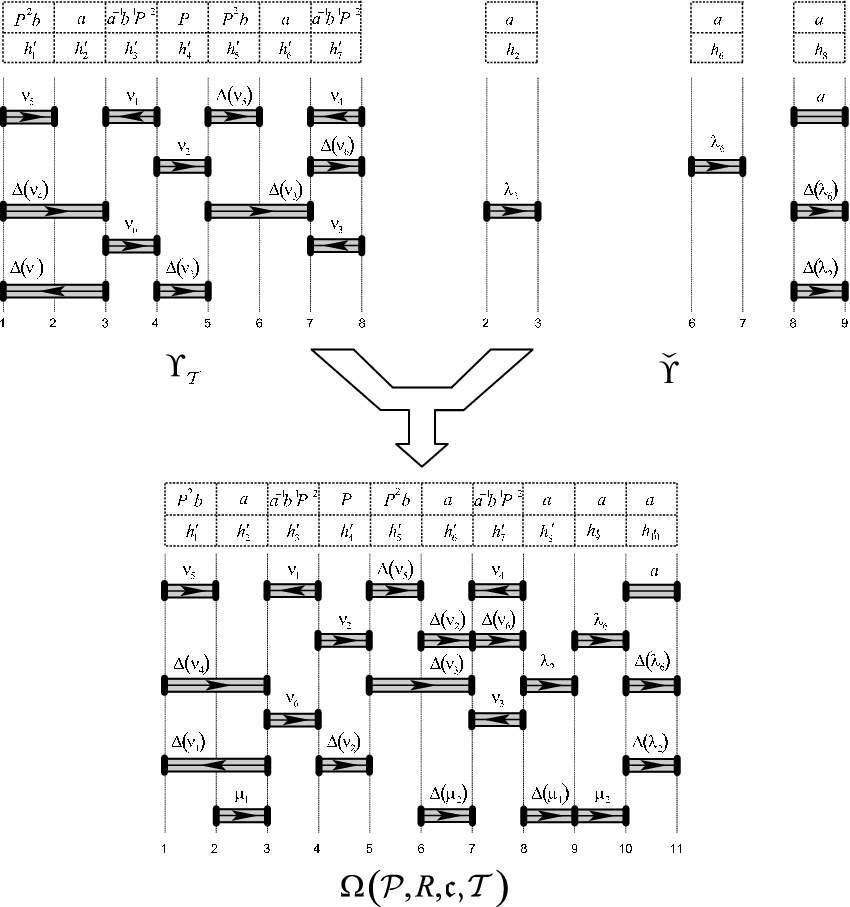
8.3. The extension tree
Recall that the coordinate group associated to a final leaf of is either a proper epimorphic image of or all the sections of the corresponding generalised equation are non-active constant sections. Since partially commutative groups are equationally Noetherian and thus any sequence of proper epimorphisms of coordinate groups is finite, an inductive argument for those leaves of that are proper epimorphic image of shows that we can construct a tree with the property that for every leaf of all the sections of the generalised equation are non-active constant sections.
We summarise the results of this section in the proposition below.
Proposition 8.2.
For a (constrained) generalised equation , one can effectively construct a finite oriented rooted at tree , , such that:
- (1)
The tree is a subtree of the tree .
- (2)
To every vertex of we assign a recursive group of automorphisms .
- (3)
For any solution of a generalised equation there exists a leaf of the tree , , and a solution of the generalised equation such that
- •
, where ;
- •
the sections of are non-active constant sections.
- •
We define a new transformation , which we call a leaf-extension of the tree at the leaf in the following way. If there are active sections in the generalised equation , we take the union of two trees and and identify the leaf of with the root of the tree , i.e. we extend the tree by gluing the tree to the vertex . If all the sections of the generalised equation are non-active, then the vertex is a leaf and consists of a single vertex, namely . We call such a vertex terminal.
We use induction to construct the extension tree . Let be a non-terminal leaf of . Apply the transformation to obtain a new tree . If in there exists a non-terminal leaf , we apply the transformation , and so on. By induction we construct a strictly increasing sequence of finite trees
| (58) |
Sequence (58) is finite. Indeed, assume the contrary, i.e. the sequence is infinite and hence the union of this sequence is an infinite tree locally finite tree. By König’s lemma, has an infinite branch. Observe that along any infinite branch in one has to encounter infinitely many proper epimorphisms. This derives a contradiction with the fact that is equationally Noetherian.
Denote by the last term of the sequence (58).
The groups of automorphisms associated to vertices of are induced, in a natural way, by the groups of automorphisms associated to vertices of the decomposition trees.
Naturally, we call leaves such that the paths associated to solutions of end in , final leaves of .
9. The solution tree and the main theorem.
In the previous section we have shown that the generalised equations associated to the final leaves of contain only non-active constant sections. In other words, the coordinate group is isomorphic to
In general, the coordinate group may be not fully residually , see the example given in Section 9.1.
The solution tree is constructed from the tree by adding some edges, labelled by homomorphisms of the coordinate groups, to final leaves of the tree . The new vertices connected to a final leaf of by an edge have the coordinate groups associated to them and satisfy the following properties.
- (1)
For every solution of , there exist a vertex and a solution such that the following diagram commutes:
- (2)
For every solution solution there exists a homomorphism such that the following diagram commutes:
- (3)
The coordinate group is a fully-residually free partially commutative group.
The idea behind this construction is the following.
Let be a final leaf of the tree and be the constrained generalised equation associated to . By definition, for any , such that , one has that for any solution of , i.e. and , see Section 2.5. Therefore, any solution of the generalised equation maps and into disjoint canonical parabolic subgroups of that -commute.
We encode all canonical parabolic subgroups of the group and the -commutativity relation between them in the graph . There are only finitely many tuples of canonical parabolic subgroups, where the solution of may map the tuple of variables . The choice of the tuple of canonical parabolic subgroups is encoded by the graph homomorphism defined below. There is a vertex in the tree for every such homomorphism .
Using the homomorphism , we construct the coordinate group that we associate to the vertex and define solutions corresponding to this vertex.
We refer the reader to Section 9.1 for an example of the constructions described in this section.
Define a non-oriented graph as follows. The set of vertices is the set of all full subgraphs of the commutation graph of (or, which is equivalent, canonical parabolic subgroups of the group ). There is an edge between two vertices and if and only , .
Let be the generalised equation associated to a final leaf of the tree . Define a non-oriented graph as follows. The set of vertices is . There is an edge between two vertices and if and only
Consider the set of all graph homomorphisms from to that satisfy the following conditions:
- (I)
, for all ;
- (II)
for every we have , i.e. does not collapse edges.
Note that the set of all such homomorphisms is finite and can be effectively constructed.
For every homomorphism we construct a new leaf in the tree and an edge joining and .
The coordinate group associated to the vertex is obtained as follows. Let be the graph product of groups with the underlying commutation graph .
The group associated to the vertex of is defined as follows. For every vertex of we consider the partially commutative group , where is the canonical parabolic subgroup of corresponding to the full subgraph of associated to . Consider the decomposition of of the form (1):
Let be the set of vertices such that . We treat every as a tuple of variables , . Consider the group
| (59) |
where if is free abelian, then , where is the free abelian group with basis , and if is non-abelian, then . The group we associate to the vertex is the group given in (59). It follows, since the graph product of partially commutative groups is again a partially commutative group, that is a free partially commutative group.
We now turn the group into a -group as follows
where the relations in identify the subgroups with the corresponding subgroups of . This is the group that we associate to the leaf of the tree . Note that, since is a partially commutative group and the centraliser of a canonical parabolic subgroup is again a canonical parabolic subgroup, the group is a free partially commutative group.
A -homomorphism from to such that for every one has is termed a solution associated to the vertex . In other words, by taking restrictions, every solution associated to the vertex , induces a tuple of homomorphisms , where is a -homomorphism from to . Conversely, any -tuple of -homomorphisms from to uniquely defines a solution associated to the vertex . The homomorphisms are called components of .
Every homomorphism , in turn, induces an -tuple of -homomorphisms from to , . Conversely, any -tuple of -homomorphisms from to uniquely defines a component of a solution .
The map induces a -homomorphism from to . Indeed, by Proposition 9.1 below, is -discriminated by . Then, by Theorem 2.4, is the coordinate group of an irreducible algebraic set. Since every equation from the system is mapped to the trivial element of and since is a coordinate group, is a homomorphism.
It follows, therefore, that property (2) described in the beginning of this section holds, i.e. that for every solution solution there exists a homomorphism such that the following diagram commutes:
It suffices to take to be the composition of and .
We now prove that property (1) described in the beginning of this section holds, i.e. that for every solution of there exists and a solution associated to the vertex such that the following diagram is commutative:
Given a solution of , we construct a non-oriented graph . There are two types of vertices in . For every , we add a vertex labelled by . For all distinct sets , we introduce a vertex of labelled by a full subgraph of generated by . There is an edge between two vertices corresponding to the sets and if and only if . There is an edge between two vertices corresponding to and if and only if . There is an edge between two vertices , corresponding to the set , and , corresponding to , if and only if . By construction, the graph is a full subgraph of .
The map , where is labelled by the full subgraph of generated by and , where extends, to an epimorphism from to . Since is a solution of , if , then . Thus, the homomorphism satisfies the property (II) above and hence, for some . Setting , it follows that the above diagram is commutative.
The proposition below proves that property (3) described in the beginning of this section holds.
Proposition 9.1.
In the above notation, the groups are -discriminated by by the family of solutions associated to the vertex .
Proof.
We use induction on the number of vertices of the underlying graph of the graph product to prove that the group is obtained from by a chain of extension of centralisers of directly indecomposable canonical parabolic subgroups. It then follows, by Proposition 2.12, that the group is -discriminated by .
If , then
where the relations in identify the subgroups with the corresponding subgroups of .
We use induction on to prove that the group is obtained from by a chain of extension of centralisers of directly indecomposable canonical parabolic subgroups. If , then the statement is trivial.
Let
Without loss of generality we may assume that , . It suffices to show that is isomorphic to
| (60) |
Since, by induction, is a partially commutative group, by Theorem 2.5,
Comparing the presentations of and the one given in (60), the statement follows in the case when .
Take a graph with vertices and consider a full subgraph of such that . By induction, the -group constructed by the graph is a partially commutative group obtained from by a sequence of extensions of centralisers of directly indecomposable canonical parabolic subgroups.
Suppose first that is directly indecomposable. Without loss of generality we may assume that , . We now prove that is isomorphic to
Since, by induction, is a partially commutative group, by Theorem 2.5,
Comparing the presentations of and , the statement follows.
If the group is directly decomposable, the proof is analogous to the base of induction and the previous case. ∎
The solution tree is obtained from the extension tree by extending every final leaf of as above. To each non-leaf vertex of the tree , we associate the same group of automorphisms as in the extension tree . For every leaf of we associate the trivial group of automorphisms.
We are now ready to formulate the main result of this paper.
Theorem 9.2.
Let be a constrained generalised equation in variables . Let be the solution tree for . Then the following statements hold.
- (1)
For any solution of the generalised equation there exist: a path in from the root vertex to a leaf , a sequence of automorphisms , where and a solution associated to the vertex , such that
(61) - (2)
For any path in from the root vertex to a leaf , any sequence of automorphisms , , and any solution associated to the vertex , the homomorphism is a solution of . Moreover, every solution of can be obtained in this way.
Proof.
The statement follows from the construction of the tree . ∎
We call leaves of the tree such that there exists a path from to as in statement (1) of Theorem 9.2 final leaves of the tree .
Theorem 9.3.
Let be the free partially commutative group with the underlying commutation graph and let be a finitely generated (-)group. Then the set of all (-)homomorphisms (, correspondingly) from to can be effectively described by a finite rooted tree. This tree is oriented from the root, all its vertices except for the root and the leaves are labelled by coordinate groups of generalised equations. The final leaves of the tree are labelled by fully residually partially commutative groups .
Edges from the root vertex correspond to a finite number of (-)homomorphisms from into coordinate groups of generalised equations. To each vertex group we assign the group of automorphisms . Each edge (except for the edges from the root and the edges to the final leaves) in this tree is labelled by an epimorphism, and all the epimorphisms are proper. Every (-)homomorphism from to can be written as a composition of the (-)homomorphisms corresponding to the edges, automorphisms of the groups assigned to the vertices, and a (-)homomorphism , into , where and is the free partially commutative subgroup of defined by some full subgraph of .
Proof.
Suppose first that is the finitely generated -group -generated by , i.e. is generated by . Let be the set of defining relations of . We treat as a system of equations (possibly infinite) over (with coefficients from ). Since is equationally Noetherian, there exists a finite subsystem such that . Since every -homomorphism from to factors through , it suffices to describe the set of all homomorphisms from to . We now run the process for the system of equations . Since there is a one-to-one correspondence between solutions of the system and homomorphisms from to , by Theorem 9.2, we obtain a description of .
Suppose now that is not a -group, (note that the set may be infinite). We treat as a coefficient-free system of equations over . Though, formally, coordinate groups are -groups, in this case, we consider instead the group , where and the intersection is taken over all homomorphisms from to such that . It is clear that is a residually group. Since is equationally Noetherian, there exists a finite subsystem such that . Every homomorphism from to factors through , it suffices to describe the homomorphisms from to . We now run the process for the system of equations and construct the solution tree, where to each vertex instead of we associate and the corresponding epimorphisms, homomorphisms and automorphisms are defined in a natural way. We thereby obtain a description of the set . ∎
9.1. Example
Let be the partially commutative group whose commutation graph is a path of length , . Consider the following coordinate group, that, a priori, could be associated to the leaf of the extension tree:
We show that the group is not fully residually . We first show that the elements and are non-trivial in . By the definition of the radical, it suffices to show that there exist homomorphisms , from to such that and . It is easy to check that the map , , and induces a homomorphism such that . Similarly, the map , , and induces a homomorphism such that .
We claim that the family of elements from can not be discriminated into , i.e. for every homomorphism from to either or . In the proof we make a substantial use of the Centraliser Theorem, see Theorem 2.5.
Indeed, since and , we have that . There are three cases to consider: either or (and ) or .
Suppose that (or, , ). Since (correspondingly, ), it follows that . Similarly, we get that , and therefore .
Suppose that . Then either or or . If or , then and thus . Finally, assume that . It follows that either or or . If , then . If or , then since , it follows that , therefore, .
Therefore, the group is not -discriminated by .
Note that the set of solutions of the generalised equation is empty, while there are solutions of the system . Indeed, if is a solution of , then , therefore . On the other hand, since , we get that . This derives a contradiction since .
Let be the partially commutative group whose commutation graph is a path of length , . Consider the following coordinate group:
We now construct one of the groups . The corresponding graphs and constructed by and are shown on Figure 20.

The set of all homomorphisms from to that satisfy properties (I) and (II) are listed in the table below:
Consider the homomorphism then the corresponding graph is a path of length , whose vertices , and are labelled by the subgroups of generated by , and correspondingly, see Figure 21. The partially commutative groups , and are directly indecomposable (the first one is free, and the latter two are cyclic), thus their decompositions of the form (1) are trivial. The set of vertices such that is . Analogously, and . The corresponding group is a graph product whose underlying graph is a path of length two and the corresponding vertex groups are , and , see Figure 21.

We then construct the coordinate group
The coordinate group is the fully residually partially commutative group, whose underlying commutation graph is shown on Figure 22.
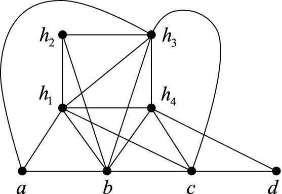
References
- [Ad75] S. I. Adian, Burnside problem and identities in groups, Science, Moscow, 1975.
- [Al07] E. Alibegović, Makanin-Razborov diagrams for limit groups, Geom. Topol. 11 (2007) pp. 643-666.
- [Ap68] K. I. Appel, One-variable equations in free groups, Proc. Amer. Math. Soc. 19 (1968), pp. 912-918.
- [Bass91] H. Bass, Groups acting on non-archimedian trees, Arboreal group theory, 1991, pp. 69-130.
- [B74] G. Baumslag, Reviews on infinite groups as printed in Mathematical Reviews 1940 through 1970, volumes 1-40 inclusive, Part 1, American Mathematical Society 1974.
- [BMR99] G. Baumslag, A. G. Myasnikov, V. N. Remeslennikov, Algebraic geometry over groups I. Algebraic sets and Ideal Theory, J. Algebra 219 (1999), pp. 16-79.
- [BMR02] G. Baumslag, A. G. Myasnikov, V. N. Remeslennikov, Discriminating Completions of Hyperbolic Groups, Geom. Dedicata 92 (2002), pp. 115-143.
- [BB97] M. Bestvina, N. Brady, Morse theory and finiteness properties of groups, Invent. Math. 129 (1997), pp. 445-470.
- [BF95] M. Bestvina, M. Feighn, Stable actions of groups on real trees, Invent. Math., 121 (1995), no. 2, pp. 287-321.
- [Bl99]
P. E. Black, ed. Algorithms and Theory of Computation Handbook, CRC Press LLC, 1999, “divide and marriage before conquest”, in Dictionary of Algorithms and Data Structures, U.S. National Institute of Standards and Technology, Available from:
http://www.nist.gov/dads/HTML/dividemarrig.html - [BGM06] D. Bormotov, R. Gilman, A. Myasnikov, Solving One-Variable Equations in Free Groups, arXiv:math/0607176v1 [math.GR]
- [Br77] R. Bryant, The verbal topology of a group, J. Algebra, 48 (1977), pp. 340-346.
- [Bul70] V. K. Bulitko, Equations and inequalities in a free group and a free semigroup. (Russian), Tul. Gos. Ped. Inst. Učen. Zap. Mat. Kaf. no. 2 Geometr. i Algebra (1970), pp. 242-252.
- [CK07] M. Casals-Ruiz, I. Kazachkov, Elements of Algebraic Geometry and the Positive Theory of Partially Commutative Groups, Canad. J. Math., to appear, arXiv:0710.4077v1 [math.GR]
- [ChKe73] C. C. Chang, H. J. Keisler, Model Theory, North-Holland, London, N.Y, 1973.
- [Ch98] O. Chapuis, On the theories of free solvable groups, J. Pure Appl. Algebra 131 (1998), pp. 13-24.
- [Char07] R. Charney, An introduction to right-angled Artin groups, Geom. Dedicata 125 (2007), pp. 141-158.
- [CCV07] R. Charney, J. Crisp, K. Vogtmann, Automorphisms of 2-dimensional right-angled Artin groups, Geom. Topol. 11 (2007), pp. 2227-2264.
- [CR00] I.M.Chiswell, V.N.Remeslennikov, Equations in Free Groups with One Variable: I, J. Group Theory 3 (2000), pp. 445-466.
- [Com81] L. P. Comerford, Quadratic equations over small cancellation groups, J. Algebra 69 (1981), no. 1, pp. 175-185.
- [ComEd81] L. P. Comerford, C. C. Edmunds, Quadratic equations over free groups and free products, J. Algebra 68 (1981), no. 2, pp. 276-297.
- [ComEd89] L. P. Comerford, C. C. Edmunds, Solutions of equations in free groups, Walter de Gruyter, Berlin, New York, 1989.
- [CW04] J. Crisp and B. Wiest, Embeddings of graph braid groups and surface groups in right-angled Artin groups and braid groups, Algebr. Geom. Topol. 4 (2004), pp. 439-472.
- [Cul81] M. Culler, Using surfaces to solve equations in free groups, Topology 20 (1981), no. 2, pp. 133-145.
- [Dahm05] F. Dahmani, Existential questions in (relatively) hyperbolic groups, arXiv:math/0505345v4 [math.GR]
- [Day08a] M. Day, Peak reduction and finite presentations for automorphism groups of right-angled Artin groups, arXiv:0807.4799v1 [math.GR]
- [Day08b] M. Day, Symplectic structures on right-angled Artin groups: between the mapping class group and the symplectic group, arXiv:0807.4801v1 [math.GR]
- [DGH01] V. Diekert, C. Gutiérrez, C. Hagenah, The existential theory of equations with rational constraints in free groups is PSPACE-complete, Inform. and Comput. 202 (2005), pp. 105-140.
- [DL04] V. Diekert, M. Lohrey, Existential and Positive Theories of Equations in Graph Products, Theory Comput. Syst. 37 (2004), pp. 133-156.
- [DMM99] V. Diekert, Yu. Matiyasevich, A. Muscholl Solving word equations modulo partial commutations, Theoret. Comput. Sci. 224 (1999), pp. 215-235.
- [DM06] V. Diekert, A. Muscholl Solvability of Equations in Graph Groups is Decidable, Internat. J. Algebra Comput. 16 (2006), pp. 1047-1069.
- [DK93] G. Duchamp, D. Krob, Partially Commutative Magnus Transformations, Internat. J. Algebra Comput. 3 (1993), 15-41.
- [Dun07] A. J. Duncan, Exponential genus problems in one-relator products of groups, Mem. Amer. Math. Soc. no. 873 (2007).
- [DKR06] A. J. Duncan, I. V. Kazachkov, V. N. Remeslennikov, Centraliser dimension and universal classes of groups, SEMR 3 (2006), pp. 197-215.
- [DKR07] A. Duncan, I. Kazachkov, V. Remeslennikov, Parabolic and quasiparabolic subgroups of free partially commutative groups, J. Algebra, 318 (2007), pp. 918-932.
- [DKR08] A. J. Duncan, I. V. Kazachkov, V. N. Remeslennikov, Automorphisms of Partially Commutative Groups I: Linear Subgroups, arXiv:0803.2213v1 [math.GR]
- [Edm75] C. C. Edmunds, On the endomorphism problem for free groups, Comm. Algebra 3 (1975), pp. 1-20.
- [Edm77] C. C. Edmunds, On the endomorphism problem for free groups II, Proc. London Math. Soc. 38 (1979), pp. 153-168.
- [Eis99] D. Eisenbud, Commutative Algebra with a View Toward Algebraic Geometry, Springer, 1999.
- [EKR05] E. S. Esyp, I. V. Kazachkov and V. N. Remeslennikov, Divisibility Theory and Complexity of Algorithms for Free Partially Commutative Groups, In: Groups, Languages, Algorithms. Contemp. Math. 378 (2005), 319-348.
- [Ful04] S. Fulthorp, Genus n Forms over Hyperbolic Groups, M.Sc. Thesis, University of Newcastle upon Tyne, 2004.
- [GLP94] D. Gaboriau, G. Levitt, F. Paulin, Pseudogroups of isometries of and Rips’ theorem on free actions on -trees, Israel J. Math., 87 (1994), 403-428.
- [Gr90] E. R. Green Graph products of groups, PhD Thesis, University of Leeds, 1990.
- [GK89] R. I. Grigorchuk, P. F. Kurchanov, On quadratic equations in free groups, Proceedings of the International Conference on Algebra, Part 1 (Novosibirsk, 1989), pp. 159-171; Contemp. Math. 131, Part 1, Amer. Math. Soc., Providence, RI, 1992.
- [GrL92] R. I. Grigorchuk, I. G. Lysënok, A description of solutions of quadratic equations in hyperbolic groups, Internat. J. Algebra Comput. 2 (1992), no. 3, pp. 237-274.
- [GPR07] M. Gutierrez, A. Piggott, K. Ruane On the automorphisms of a graph product of abelian groups, arXiv:0710.2573v1 [math.GR]
- [Gr05] D. Groves, Limit groups for relatively hyperbolic groups, II: Makanin-Razborov diagrams, Geom. Topol. 9 (2005), pp. 2319-2358.
- [Gr08] D. Groves, Limit groups for relatively hyperbolic groups, I: The basic tools, arXiv:0412492v2 [math.GR].
- [Guba86] V. Guba Equivalence of infinite systems of equations in free groups and semigroups to finite subsystems. Mat. Zametki, 40 (1986), pp. 321-324.
- [HW08] F. Haglund, D. Wise, Special Cube Complexes, Geom. Funct. Anal. 17 (2008), pp. 1551-1620.
- [HNN49] G. Higman, B. Neumann, H. Neumann, Embedding Theorems for Groups, J. London Math. Soc. s1-24 (1949), no.4, pp. 247-254
- [Hm71] Yu. I. Hmelevskiĭ, Systems of equations in a free group. I, (Russian), Izv. Akad. Nauk. Ser. Mat., 35 (1971), no. 6, pp. 1237-1268; translation in Math. USSR Izv. 5 (1971), pp. 1245-1276.
- [Hm72] Yu. I. Hmelevskiĭ, Systems of equations in a free group. II, (Russian), Izv. Akad. Nauk. Ser. Mat., 36 (1972), no. 1, pp. 110-179, translation in Math. USSR Izv. 6 (1972), pp. 109-180.
- [Hum94] S. Humphries, On representations of Artin groups and the Tits conjecture, J. Algebra 169 (1994), pp. 847-862.
- [Kaz07] I. Kazachkov, Algebraic Geometry over Lie Algebras, Surveys in Contemporary Mathematics, LMS Lecture Notes, Volume 347 (2007), 34-81
- [KhLMT08] O. Kharlampovich, I. G. Lysënok, A. G. Myasnikov, N. W. M. Touikan, Quadratic equations over free groups are NP-complete, arXiv:0802.3839v1 [math.GR]
- [KhM98a] O. Kharlampovich, A. Myasnikov, Irreducible affine varieties over a free group I: Irreducibility of quadratic equations and Nullstellensatz, J. Algebra, 200 (1998), pp. 472-516.
- [KhM98b] O. Kharlampovich, A. Myasnikov, Irreducible affine varieties over a free group II: Systems in triangular quasi-quadratic form and description of residually free groups, J. of Algebra, 200 (1998), pp. 517-570.
- [KhM05a] O. Kharlampovich, A. Myasnikov, Implicit function theorem over free groups, J. Algebra, 290 (2005), pp. 1-203.
- [KhM05b] O. Kharlampovich, A. Myasnikov, Effective JSJ Decompositions, In: Groups, Languages, Algorithms. Contemp. Math. 378 (2005), pp. 87-212.
- [KhM06] O. Kharlampovich, A. Miasnikov, Elementary theory of free non-abelian groups, J.Algebra, 302 (2006), pp. 451-552.
- [LS08]
M. Lohrey, G. Sénizergues, Equations in HNN extensions, preprint,
http://inf.informatik.uni-stuttgart.de/fmi/ti/personen/Lohrey/HNN.html - [Lor63] A. A. Lorents, The solution of systems of equations in one unknown in free groups, Dokl. Akad. Nauk 148 (1963), pp. 1253-1256.
- [Lor68] A. A. Lorents, Representations of sets of solutions of systems of equations with one unknown in a free group, Dokl. Akad. Nauk 178 (1968), pp. 290-292.
- [Lyn60] R. C. Lyndon, Equations in free groups, Trans. Amer. Math. Soc. 96 (1960), pp.445-457.
- [Lyn80] R. Lyndon, Equations in groups, Bull. Braz. Math. Soc. (N.S.) 11 (1980), pp. 79-20
- [LS77] R. C. Lyndon, P. E. Schupp, Combinatorial group theory, Springer, 1977.
- [Lys88] I. G. Lysënok, Solutions of quadratic equations in groups with the small cancellation condition, (Russian) Mat. Zametki 43 (1988), no. 5, pp. 577-592; translation in Math. Notes 43 (1988), no. 5-6, pp. 333-341
- [Mak77] G. S. Makanin, The problem of solvability of equations in a free semigroup, Mat. Sb. (N.S.), 1977, 103(145):2(6), pp. 147-236.
- [Mak82] G. S. Makanin, Equations in a free group (Russian), Izv. Akad. Nauk SSSR, Ser. Mat., 46 (1982), pp. 1199-1273, transl. in Math. USSR Izv., 21 (1983)
- [Mak84] G. S. Makanin, Decidability of the universal and positive theories of a free group (Russian), Izv. Akad. Nauk SSSR, Ser. Mat., 48 (1985), pp. 735-749, transl. in Math. USSR Izv., 25 (1985).
- [Mal62] A. I. Malcev. On the equation in a free group Algebra i Logika Sem. 1 (1962), no. 5, pp. 45-50.
- [Mat97] Yu. Matiyasevich, Some decision problems for traces, In S. Adian and A. Nerode, editors, Proceedings of the 4th International Symposium on Logical Foundations of Computer Science (LFCS’97), Yaroslavl, Russia, July 6-12, 1997, number 1234 in Lecture Notes in Computer Science, pp. 248-257, Berlin Heidelberg, 1997, Springer-Verlag, Invited lecture.
- [McC75] J. McCool, Some finitely presented subgroups of the automorphism group of a free group, J. Algebra 35 (1975), pp. 205-213.
- [Mer66] Yu. I. Merzlyakov. Positive formulae on free groups. Algebra i Logika 5 (1966), pp. 25-42.
- [MR96] A. G. Myasnikov, V. N. Remeslennikov, Exponential groups 2: extension of centralizers and tensor completion of CSA-groups, Internat. J. Algebra Comput., 6 (1996), pp. 687-711.
- [MR00] A. G. Myasnikov, V. N. Remeslennikov, Algebraic geometry over groups II. Logical Foundations. J. Algebra 234 (2000), pp. 225-276.
- [Niel] J. Nielsen, Die Isomorphismen der allgemeinen, unendlichen Gruppe mit zwei Erzeugenden, Math. Ann. 78 (1918), pp. 385-397.
- [Oj83] Yu. I. Ozhigov, Equations in two variables over a free group, Dokl. Akad. Nauk, 268 (1983), no. 4, pp. 809-813.
- [Ol89] A. Yu. Ol’shanskii, Diagrams of homomorphisms of surface groups, (Russian) Sibirsk. Mat. Zh. 30 (1989), no. 6, pp. 150-171; translation in Siberian Math. J. 30 (1989), no. 6, pp. 961-979.
- [Pl99a] W. Plandowski, Satisfiability of word equations with constants is in NEXPTIME, In Theory of Computing (STOC 99), pp. 721-725. ACM 49. Press.
- [Pl99b] W. Plandowski, Satisfiability of word equations with constants is in PSPACE, In Foundations of Computer Science (FOCS 99), pp. 495-500. IEEE Computer Society Press.
- [Raz84] A. A. Razborov, An equation in a free group whose set of solutions does not allow a representation as a superposition of a finite number of parametric functions, In: Proceedings of the 9th All-Union Symposium on Group Theory, Moscow, 1984, p. 54.
- [Raz85] A. A. Razborov, On systems of equations in a free group, Math. USSR, Izvestiya, 25 (1985), pp. 115-162.
- [Raz87] A. A. Razborov, On systems of equations in a free group, PhD thesis, Steklov Math. Institute, Moscow, 1987.
- [Raz95] A. A. Razborov On systems of equations in free groups, in Combinatorial and geometric group theory. Edinburgh 1993, pp. 269-283, Cambridge University Press, 1995.
- [Rem89] V. N. Remeslennikov, -free groups, Siberian Math. J., 30 (1989), no. 6, pp. 153-157.
- [Rep83] N. N. Repin, Equations with one unknown in nilpotent groups, (Russian) Mat. Zametki 34 (1983), no. 2, pp. 201-206, English translation in Math. Notes 34 (1983), no. 1-2, pp. 582-585.
- [Rep84] N. N. Repin, Solvability of equations with one indeterminate in nilpotent groups (Russian) Izv. Akad. Nauk SSSR Ser. Mat. 48 (1984), no. 6, pp. 1295-1313.
- [RS95] E. Rips, Z. Sela, Canonical representatives and equations in hyperbolic groups, Invent. Math. 120, pp. 489-512.
- [RS97] E. Rips, Z. Sela, Cyclic splittings of finitely presented groups and the canonical JSJ decomposition, Ann. of Math., 146 (1997), pp. 53-109.
- [Rom77] V. A. Roman’kov, Unsolvability of the endomorphic reducibility problem in free nilpotent groups and in free rings (Russian) Algebra i Logika 16 (1977), no. 4, pp. 457-471; English translation in: Algebra and Logic, 16 (1977), no. 4, pp. 310-320.
- [Rom79a] V. A. Roman’kov, Universal theory of nilpotent groups, (Russian), Mat. Zametki 25 (1979), no. 4, pp. 487-495.
- [Rom79b] V. A. Roman’kov, On equations in free metabelian groups, Siberian Math. J. 20 (1979), no. 3, pp. 671-673.
- [Sch90] K. Schulz, Makanin’s Algorithm for Word Equations - Two Improvements and a Generalization, Proceedings of the First International Workshop on Word Equations and Related Topics, pp. 85-150, 1990.
- [Sch69] P. E. Schupp, On the substitution problem for free groups, Proc. Amer. Math. Soc. 23 (1969), pp. 421-24.
- [Sela97] Z. Sela, Structure and rigidity in (Gromov) hyperbolic groups and discrete groups in rank 1 Lie groups, II, Geom. Funct. Anal. 7 (1997), 561-593.
- [Sela01] Z. Sela, Diophantine geometry over groups I: Makanin-Razborov diagrams, Publ. Math. Inst. Hautes Études Sci. 93 (2001), pp. 31-105.
- [Sela03] Z. Sela, Diophantine geometry over groups II: Completions, closures and formal solutions, Israel J. Math. 134 (2003), pp. 173-254.
- [Sela06] Z. Sela, Diophantine geometry over groups VI: The elementary theory of a free group, Geom. Funct. Anal. 16 (2006), 707-730.
- [Sela02]
Z. Sela, Diophantine geometry over groups VII: The elementary theory of a hyperbolic group, preprint,
http://www.ma.huji.ac.il/~zlil/hyp.dvi - [Ser89] H. Servatius, Automorphisms of Graph Groups, J. Algebra, 126 (1989), no. 1, pp. 34-60.
- [Sh05] S. L. Shestakov, The equation in partially commutative groups, Siberian Math. J., 46 (2005), pp. 364-372; translation in Siberian Math. J., 46 (2005), no. 2, pp. 364-372.
- [Sh06] S. L. Shestakov, The equation in partially commutative groups, Sibirsk. Mat. Zh., 47 (2006), no.2, pp. 463-472; translation in Siberian Math. J., 47 (2006), no. 2, pp. 383-390.
- [T08] N. Touikan, On the coordinate groups of irreducible systems of equations in two variables over free groups, arXiv:0810.1509v1 [math.GR]
- [VW94] L. Van Wyk, Graph groups are biautomatic, J. Pure Appl. Algebra 94 (1994), no.3, pp. 341-352.
- [Vd97] A. Vdovina, Products of Commuators in Free Products, Inter. Jour. of Alg. and Computation, 7 (1997), no. 4, pp. 471-485.
- [Wic62] M. J. Wicks, Commutators in Free Products, J. London Math. Soc. 37 (1962), pp. 433-444.
Index
- algebraic set §2.2
- automorphism
- completely induced Definition 7.2
- dual Definition 7.2
- invariant with respect to the kernel §7.1
- invariant with respect to the kernel in the sense of Razborov §7.1
- invariant with respect to the non-quadratic part §7.1
- invariant with respect to the non-quadratic part in the sense of Razborov §7.1
- tame Remark 7.3
- base
- active Definition 4.1
- belongs to a section Definition 3.8
- carrier §4.3
- constant item 1
- contained in another base Definition 3.8
- contains an item Definition 3.8
- dual item 1
- eliminable §4.3
- intersects another base Definition 3.8
- leading §4.3
- linear Definition 3.8
- non-active Definition 4.1
- of a generalised equation item 1
- overlaps with another base Definition 3.8
- quadratic §7.1
- quadratic-coefficient §7.1
- transfer §4.3
- variable item 1
- block §2.5
- boundary
- closed Definition 3.8
- free Definition 3.8
- intersects a base Definition 3.8
- of a generalised equation item 2
- open Definition 3.8
- tied Definition 3.8
- touches a base Definition 3.8
- -tied Definition 3.8
- boundary connection item 4
- cancellation divisor §5
- cancellation matrix Definition 5.4
- canonical homomorphism of coordinate groups of generalised equations §4.4
- canonical parabolic subgroup §2.5
- carrier §4.3
- clan §2.6
- complexity of the generalised equation Definition 4.14
- coordinate group
- of a system of equations §2.2
- of an algebraic set §2.2
- of the (constrained) generalised equation Definition 3.15
- cyclically reduced element §2.5
- dependence graph §2.6
- -discriminated group §2.4
- divisor of an element §2.5
- elimination of a base §4.3
- elimination process for a generalised equation §4.3
- equation of a generalised equation
- equation over a group §2.2
- -equationally Noetherian group §2.2
- equivalence
- of generalised equations Definition 3.2
- of systems of equations §2.2
- excess of the solution Definition 4.8
- exponent
- formula
- -fully residually group §2.4
- generalised equation §3.1
- combinatorial Definition 3.1
- constrained Definition 3.4
- formally consistent Definition 3.9
- periodised Definition 6.9
- quadratic §4.3
- regular with respect to a periodic structure Definition 6.15
- singular with respect to a periodic structure Definition 6.15
- strongly singular with respect to a periodic structure Definition 6.15
- geodesic §2.5
- global position §2.6
- graph
- commutation, of a partially commutative group §2.5
- non-commutation, of a partially commutative group §2.5
- of a periodic structure Definition 6.7
- graph group §2.5
- graph product of groups §2.5
- -group §2.2
- finitely generated §2.2
- height
- -homomorphism §2.2
- irreducible
- isomorphism of algebraic sets §2.2
- item
- active Definition 4.1
- belongs to a base Definition 3.8
- belongs to a section Definition 3.8
- belongs to the kernel §4.3
- constant Definition 3.8
- covered times Definition 3.8
- free Definition 3.8
- linear Definition 3.8
- non-active Definition 4.1
- of a generalised equation §3.1
- quadratic Definition 3.8
- kernel of a generalised equation §4.3
- leaf
- left-divide §2.5
- length §2.5
- of a solution of the generalised equation Definition 3.7
- letter §2.5
- median position §2.6
- morphism of algebraic sets §2.2
- normal form §2.6
- occurrence §2.5
- pair of matched bases Definition 3.8
- part of a generalised equation
- active Definition 4.1
- non-active Definition 4.1
- non-quadratic §7.1
- quadratic §7.1
- partially commutative group §2.5
- -partition table §3.2.1
- path
- defined by a solution in the tree §4.4
- §7, §7.3
- prohibited of type 12 Definition 7.8
- prohibited of type 15 Definition 7.13
- prohibited of type 7-10 Definition 7.8
- -reducing §7.2
- period §6.1
- (-)periodic word §6.1
- periodic structure Definition 6.3
- connected §6.1
- regular Definition 6.15
- singular Definition 6.15
- strongly singular
- of type (a) Definition 6.15
- of type (b) Definition 6.15
- quasi identity §2.3
- radical
- -residually group §2.4
- right-angled Artin group §2.5
- right-divide §2.5
- section Definition 3.8
- (-)periodic §6.1
- active Definition 4.1
- closed Definition 3.8
- constant Definition 4.1
- non-active Definition 4.1
- variable Definition 4.1
- sentence §2.3
- -separated group §2.4
- solution
- associated to the vertex §9
- of a constrained generalised equation Definition 3.7
- of a generalised equation
- minimal with respect to the group of automorphisms Definition 5.5
- over Definition 3.6
- over Definition 3.5
- periodic with respect to a period Definition 6.1
- of a system of equations §2.2
- source point §2.6
- standard form of a generalised equation Definition 4.2
- -subgroup §2.2
- system of equations over a group §2.2
- target point §2.6
- terminal vertex §8.3
- transformation of a generalised equation
- type
- variable of a generalised equation §3.1
Glossary of notation
- :
-
the automorphism group associated to a vertex of the trees , and , 98, 101, 105
- :
-
the active part of a generalised equation, 39
- :
-
finitely generated group of automorphisms of associated with a periodic structure on , 67
- :
-
recursive group of automorphisms associated to the root of , 85
- :
-
the subgroup of generated by all letters that do not occur in and commute with for every , 14
- :
-
the subgroup of generated by all letters that do not occur in and commute with , 14
- :
-
function from the set of bases to the set of boundaries of a generalised equation that determines the left-most boundary of a base, 20
- :
-
the set of letters that occur in a word , 14
- :
-
the set of letters that occur in , 14
- :
-
a finite alphabet, the generating set of , 14
- :
-
the set of boundary connections of a generalised equation, 20
- :
-
the set of boundaries of a generalised equation, 20
- :
-
the set of bases of a generalised equation, 20
- :
-
function from the set of bases to the set of boundaries of a generalised equation that determines the right-most boundary of a base, 20
- :
-
the set of all constant sections of a generalised equation, 38
- :
-
“short” cycles in , 64
- :
-
“free” cycles in , 64
- :
-
the set of commutators of elements of sets and , 14
- :
-
elements of sets and commute pairwise, 14
- , :
-
complexity of a generalised equation, 49
- :
-
the cancellation divisor of and , 56
- :
-
derived transformation , 44
- :
-
derived transformation , 44
- :
-
derived transformation , 44
- :
-
derived transformation , 45
- :
-
derived transformation , 47
- :
-
length of the active part of the solution, , 47
- :
-
derived transformation , 48
- :
-
involution on the set of variable bases of a generalised equation that determines the dual of a base, 20
- :
-
decomposition of the period defined by the boundary , 61
- :
-
length of the “quadratic part of the solution” , 88
- :
-
length of the “quadratic-coefficient part of the solution” , 88
- :
-
elementary transformation , 39
- :
-
elementary transformation , 40
- :
-
elementary transformation , 40
- :
-
elementary transformation , 41
- :
-
elementary transformation , 42
- :
-
exponent of periodicity of the word , 60
- :
-
a function that assigns a pair to the pair , , 86
- :
-
a function that assigns a pair to the pair , , 86
- :
-
function from the set of variable bases of a generalised equation to that determines orientation of the base, 20
- , :
-
free monoid on the alphabet , 18
- :
-
coordinate group of the system over , 11
- :
-
the set of all constrained generalised equations over constructed by -partition tables for the system , 26
- :
-
the set of all constrained generalised equations over constructed for the constrained generalised equation over , 30
- :
-
partially commutative group, 14
- :
-
partially commutative group with underlying commutation graph , 14
- :
-
coordinate group of the generalised equation , 26
- :
-
fully residually partially commutative group associated to the leaf of the solution tree , 103
- :
-
graph of a periodic structure, 62
- :
-
the subgraph of all of whose edges are “short”, , 63
- :
-
a non-oriented graph that encodes all canonical parabolic subgroups of the group and the -commutativity relation between them, 102
- , :
-
the number of bases which contain , 23
- :
-
the number of bases from that contain , 90
- :
-
a non-oriented graph that describes the canonical parabolic subgroups associated to the solution of a generalised equation, 103
- :
-
commutation graph of a partially commutative group, 14
- :
-
length of a solution of a (constrained) generalised equation, , 23
- :
-
if is a solution of a generalised equation, , 23
- , :
-
if is a solution of a generalised equation, , 23
- :
-
set of -homomorphisms from to , 10
- :
-
labels of the “short” edges of , , 63
- :
-
the product of items , 23
- :
-
the product of items , 23
- , :
-
kernel of a (constrained) generalised equation, 45
- :
-
first-order language of groups, 12
- :
-
first-order language of groups enriched by constants from , 12
- :
-
first-order language of groups enriched by constants from , 12
- :
-
free or partially commutative monoid, or , 20
- :
-
the non-active part of a generalised equation, 39
- :
-
normal closure of , 11
- :
-
the number of bases in the section , 49
- , :
-
the number of bases in the active sections of a generalised equation, 49
- :
-
is a solution of the constrained generalised equation , 23
- :
-
constrained generalised equation, 23
- :
-
constrained generalised equation, 22
- :
-
the set of all variable bases for which either or belongs to the active part of a generalised equation, 47
- , :
-
the generalised equation obtained from (or ) by , 44
- :
-
the generalised equation treated as a system of equations over the partially commutative group , 26
- :
-
excess of the solution, , 47
- :
-
non-empty set of variables, variable bases, and closed sections that belong to the periodic structure , 61
- :
-
a non-oriented graph that encodes coefficient equations of and the relation , 102
- :
-
periodic structure, 61
- :
-
homomorphism defined by the solution , 11
- :
-
periodic structure associated to a -periodic solution , 61
- :
-
radical of the system , 11
- :
-
radical of a set , 11
- :
-
set of elements related with , 10
- , , :
-
the number of items of a generalised equation, 21
- :
-
the boundary between active and non-active parts of a generalised equation, 39
- :
-
the number of free variables that belong to the non-active sections of , 83
- :
-
the cardinality of , 14
- :
-
system of equations associated to the generealised equation, 21
- :
-
section of a generalised equation, 23
- , :
-
the set of “short” edges of the graph of a periodic structure, 63
- , :
-
the set of all closed sections of a generalised equation , 38
- :
-
the section , 23
- :
-
a function that bounds the length of a minimal solution, 84
- :
-
the infinite, locally finite tree of the process, 49
- :
-
the finite subtree of that does not contain prohibited paths, 80, 85
- :
-
the decomposition tree of , 94
- :
-
the extension tree of , 99
- :
-
the solution tree of a generalised equation, 105
- , :
-
partially commutative monoid monoid on the alphabet corresponding to the group , 18
- , :
-
function of the generalised equation, 83
- :
-
type of the vertex of the tree , , , or , 54
- :
-
is a solution of the generalised equation , 23
- :
-
generalised equation, 23
- :
-
combinatorial generalised equation associated to a system of equations over a monoid, 21
- :
-
a subset of the set of generators of the coordinate group of a periodised generalised equation, 64
- :
-
generalised equation treated as a system of equations over the partially commutative group , 26
- :
-
the set of all variable sections of a generalised equation, 38
- :
-
algebraic set defined by over , 11
- :
-
a recursive group of automorphisms of that we associate to a vertex of the tree , 77
- :
-
for any word in and any solution of a generalised equation, , 23
- :
-
a geodesic of a word , , 14
- :
-
a set of generators of the coordinate group of a periodised generalised equation, 64
- :
-
the number of open boundaries in the active sections of a generalised equation, 49
- :
-
a subset of the set of generators for the coordinate group of a periodised generalised equation, 64
- ‘’:
-
reflexive, transitive relation on the set of solutions of a generalised equation, 56
- ‘’:
-
if is a solution of and is a solution of , , then if and only if , 85
- ‘’:
-
graphical equality of words, 15
- ‘’:
-
disjoint commutation of elements or sets, 14
- ‘’:
-
no cancellation in the product of and , 14