Pairing in fermionic systems: A quantum information perspective
Abstract
The notion of ”paired” fermions is central to important condensed matter phenomena such as superconductivity and superfluidity. While the concept is widely used and its physical meaning is clear there exists no systematic and mathematical theory of pairing which would allow to unambiguously characterize and systematically detect paired states. We propose a definition of pairing and develop methods for its detection and quantification applicable to current experimental setups. Pairing is shown to be a quantum correlation different from entanglement, giving further understanding in the structure of highly correlated quantum systems. In addition, we will show the resource character of paired states for precision metrology, proving that the BCS states allow phase measurements at the Heisenberg limit.
I Introduction
The notion of pairing in fermionic systems is at least as old as the seminal work of Bardeen, Cooper and Schrieffer explaining superconductivity [1]. The formation of fermionic pairs with opposite spin and momentum is not only the source for the vanishing resistance in solid state systems, but it can also explain many other interesting phenomena, like superfluidity in helium-3 or inside a neutron star.
For instance, with recent progress in the field of ultracold quantum gases fermionic pairing has gained again a lot of attention [2, 3, 4, 5, 6, 7, 8, 9]. These experiments allow an excellent control over many parameters inherent to the system, offering a unique testing ground for existing theories and an exploration of new and exotic phases. However, the notion of pairing in these systems is less clear and sometimes even controversial. Recent experiments on the BEC-BCS crossover have caused a heated debate whether or not the obtained data was in agreement with pairing [7, 10, 11, 12]. In addition, pairing without superfluidity [13] has been observed in these experiments, raising fundamental questions on quantum correlations in fermionic many-body systems.
Motivated by these exciting experiments and the central role pairing plays in many physical phenomena, and by the perceived lack of accepted criteria to verify the presence of pairing in a quantum state, we propose a clear and unambiguous definition of pairing intended to capture its two-particle nature and to allow a systematic study of the set of paired states and its properties. We employ methods and tools from quantum information theory to gain a better understanding of the set of fermionic states that display pairing. In particular, we develop tools for the systematic detection and for the quantification of pairing, which are applicable to current experiments. Our approach is inspired by concepts and methods from entanglement theory, thus building a bridge between quantum information science and condensed matter physics.
Since they contain non-trivial quantum correlations, paired states belong to the set of entangled many-body states. However, pairing will turn out to be not equivalent to any known concept of entanglement in systems of indistinguishable particles [14, 15, 16, 17, 18, 19, 20, 21, 22, 23, 24, 25, 26, 27, 28, 29] but to represent a particular type of quantum correlation of its own. We will show that these correlations can be exploited for quantum phase estimation. Hence pairing constitutes a resource in state estimation using fermions as much as entangled states with spins.
This article is organized as follows: After the introduction of the language necessary for the description of fermionic systems in Sec. II, we will introduce the general framework of pairing theory in Sec. III. This part includes our definition of pairing and methods for its detection and quantification. In order to fill the theory with life we will apply it to two different classes of fermionic states in Secs. IV and V. We start out with pairing in fermionic Gaussian states in Sec. IV. The interest in this family of states is two-fold. First, the pairing problem can be solved completely in this case, so that Gaussian states are particularly interesting from a conceptual point of view. Second, there exists a relation between pure fermionic Gaussian states and the BCS states of superconductivity (see Sec. II.4 for the details) which are examples of paired states par excellence. This enables us to translate methods developed for the detection and quantification of pairing for Gaussian states to the BCS-states. The reader interested in the application of our pairing theory to experimental application is referred to Sec. V. There we study pairing for number conserving states, i.e. states commuting with the number operator. This class includes the states appearing in the BEC-BCS crossover, and we will develop tools for the detection of pairing tailored for these systems. In VI we will show that certain classes of paired states constitute a resource for quantum phase estimation, proving that pairing is a resource similar to entanglement.
II Fermionic states
In this chapter we review the basic concepts needed for the understanding of fermionic systems. We start out with some notation used for the description of fermionic systems in second quantization in Sec. II.1. As pairing is a special sort of correlation, we continue with a review on quantum correlations and entanglement in systems of indistinguishable particles in Sec. II.2. This general part is followed by the introduction of fermionic Gaussian states and number conserving states in Secs. II.3 and II.4. The latter includes the introduction of BCS-states and their relation to the Gaussian states. As this part is only necessary for the application of the pairing theory to these concrete examples in Secs. IV and V, it is possible to skip this part at the beginning, and then refer to it later on.
II.1 Basic notation
We consider fermions on an -dimensional single particle Hilbert space . All observables are generated by the creation and annihilation operators and , which satisfy the canonical anti-commutation relations (CAR) and . We say creates a particle in mode (or single particle state) , where denotes the canonical orthonormal basis of . In general, for any normalized , we define , the annihilation operator for mode .
Sometimes a description using the hermitian Majorana operators , , which satisfy , is more convenient.
The Hilbert space of the many-body system, the antisymmetric Fock space over modes, , is spanned by the orthonormal Fock basis defined by
| (1) |
where the vacuum state fulfills . The are the eigenvalues of the the mode occupation number operators . The -particle subspace spanned by vectors of the form (1) satisfying is denoted by . The set of density operators on the Hilbert space is denoted by .
Linear transformations of the fermionic operators which preserve the CAR are called canonical transformations. They are of the form where is an element of the real orthogonal group. These transformations can be implemented by unitary operations on which are (for ) generated by quadratic Hamiltonians in the (see, e.g. [30]). The subclass of canonical operations which commute with the total particle number are called passive transformations. They take a particularly simple form in the complex representation , where is unitary on the single-particle Hilbert space , i.e., they describe (quasi)free time-evolution of independent particles. Canonical transformations which do not commute with are called active. They mix creation and annihilation operators.
II.2 Quantum correlations of fermionic states
The notion of ”pairing” used in the description of superconducting solids, superfluid liquids, baryons in nuclei, etc. is always associated with a correlated fermionic system. The subject of quantum correlations in fermionic systems is vast [31]. In recent years, there has been renewed interest from the perspective of quantum information theory. There quantum correlations (aka entanglement) of distinguishable systems (qubits) play a crucial role as a resource enabling certain state transformations or information processing tasks. The detailed quantitative analysis of quantum correlations motivated by this has proven to be valuable also in the understanding of condensed matter systems (see [32] for a review).
In contrast to the usual quantum information setting which studies the entanglement of distinguishable particles, the indistinguishable nature of the fermions is of utmost importance in the settings of our interest. The existing concepts for categorizing entanglement in systems of indistinguishable particles fall into two big classes: Entanglement of modes [14, 15, 16, 17, 18, 19, 20, 21, 22] and entanglement of particles. Entanglement of particles has been considered e.g. in [23, 24, 25, 26, 27, 28, 29], leading to the concept of Slater rank [24, 25], being the generalization of the Schmidt rank to indistinguishable particles. We show in Sec. III that our definition of pairing does not coincide with any of the existing ideas. We refrain from giving an exhaustive review on the existing concepts referring the interested reader to the mentioned literature and references therein, and restrict to the following definition:
Definition II.1.
A pure fermionic state is called a product state, if there exists a passive transformation such that
| (2) |
A state is called separable, if it can be written as the convex combination of product states, i.e.
| (3) |
where , and all are product states. All other states are said to have ”Slater number larger than 1” and are called entangled (in the sense of [24, 25]).
We denote the set of all separable states by and by the set of all separable states of particle number .
Note that the sets of separable
states are convex and invariant under passive transformations. Both properties
will be useful later on.
Separable states have only correlations resulting from
their anti-symmetric nature and classical correlations due to mixing. In the
terminology of Refs. [24, 25] they
have Slater number one and describe unentangled particles. These states will
certainly not contain correlations associated with pairing. (Note that they
can be mode-entangled for an appropriate partition of modes.)
Besides basis change, there are other operations, which do not create quantum correlations and it is useful to see that the set of separable states is invariant under them.
Lemma II.2.
Let be a separable state. Then
the state after measuring the particle number in some mode
is separable for both possible outcomes .
Furthermore, , the reduced state
obtained by tracing out the mode , is also separable.
Proof.
As is convex, it is sufficient to prove the claim for product states . Let be the vector in Hilbert space corresponding to . Our aim is to show that , where are product states and eigenstates of the occupation number operator . If is in the span of or orthogonal to it, the state already is a eigenstate and we are done. Otherwise, define orthogonal to the such that and define another orthonormal basis for the span with and [here denotes the inner product on the single particle Hilbert space]. Then we can write for some . Hence, with and which both clearly are product states. The reduced state is the statistical mixture of and and therefore clearly separable. ∎
II.3 Fermionic Gaussian states
Fermionic Gaussian states are represented by density operators that are exponentials of a quadratic form in the Majorana operators. A general multi-mode Gaussian state is of the form
| (4) |
where , is a normalization constant and is a real anti-symmetric matrix. Every anti-symmetric matrix can be brought to a block diagonal form
| (5) |
by a special orthogonal matrix .
From eq. (4) it is clear that Gaussian states have an interpretation as thermal (Gibbs) states corresponding to a Hamiltonian that is a quadratic form in the , i.e., and the form eq. (5) shows that every Gaussian state has a normal-mode decomposition in terms of single-mode “thermal states” of the form . From this one can see that the state is fully determined by the expectation values of quadratic operators and . These are collected in a convenient form in the real and anti-symmetric covariance matrix which is defined via
| (6) |
It can be brought into block diagonal form by a canonical transformation:
| (7) |
For every valid density operator, , and the
eigenvalues of are given by . Hence,
every corresponding to a physical state has to fulfill
or, equivalently,
and to each such corresponds a valid Gaussian density
operator where the relation between and is given by
. The covariance matrix of the
ground state of is obtained in the limit
i.e., . In fact, this shows
that every pure Gaussian state is the ground state to some
quadratic Hamiltonian. The purity of the state can be easily
determined from the covariance matrix as a Gaussian state is pure
if and only if
(see, e.g., [33]).
As mentioned, Gaussian states are fully characterized by their covariance
matrix and all higher correlations can be obtained from by Wick’s
theorem (see, e.g., [33]) via
| (8) |
where and is the corresponding submatrix of . is called the Pfaffian.
In some cases it is more appropriate to use a different ordering of the Majorana operators, the so-called q-p-ordering , opposed to the mode-ordering introduced at the beginning. When using the q-p-ordering, the relation between the real and complex representation is given by
| (9) |
where . The
transformation matrix fulfills .
In the q-p-ordering the covariance matrix obtains the following
block structure:
| (10) |
Finally, for some purposes it is more convenient to use the complex representation, where the covariance matrix is of the form
| (11) |
where , and denotes the complex conjugate. Note that and and hence . The condition takes the form .
The description of by its covariance matrix is especially convenient to describe the effect of canonical transformations, i.e. time evolutions generated by quadratic Hamiltonians: if in the Heisenberg picture then in the Schrödinger picture. For a passive transformation , the q-p-ordered Majorana operators transform as
| (12) |
where is the real part of the unitary , and the imaginary part. Note that is both orthogonal and symplectic. The behaviour of under a passive transformation is particularly simple: and transform according to and .
Passive transformations can be used to transform pure fermionic states to a simple standard form, the so-called Bloch-Messiah reduction [34]. The q-p ordered CM takes the form (10) where
In Hilbert space, the state in standard form is given by
| (19) |
where , , . This comprises the kind of ”paired” states appearing in the BCS theory of superconductivity [1] with , . We will refer to these states as Gaussian BCS states. We would like to stress the fact that every pure Gaussian state is a Gaussian BCS state in some basis.
II.4 Number conserving fermionic states
For the application to physical systems we are interested in states for which the particle number is a conserved quantity. We call a number conserving state if where denotes the total number operator. Thus, the density operator of a number conserving state can be written as a mixture of -eigenstates. In particular, all separable states as defined in Def. II.1 are number conserving.
The Gaussian BCS wave function (19) is not number conserving (except for the case that either or vanishes for every mode), but a relation to these states can be established via the identity
| (20) |
where the number conserving -particle BCS state is given by
| (21) |
where we have introduced the pair creation operator . The coefficients are related to and via , is a normalization constant which is seen to be
by rewriting Eq. (21) as
| (22) |
The coefficients can be interpreted as the probability amplitude
of being in state since =1. We will in general drop the term number
conserving and refer to
states of the form (21) as BCS states.
Whenever the distribution of the is sharply peaked
around some average particle number , expectation values of
relevant observables for the number conserving BCS states
are approximated well by the
expectation values of the Gaussian BCS state. This relation will
turn out very useful later on, as results on Gaussian states can
be translated into results on number conserving BCS states.
III Pairing theory
In this section we introduce a precise definition of pairing as a property of quantum states.
III.1 Motivation and statement of the definition
The simplest system in which we can find pairing consists of two particles and four modes11 1 For three modes, all pure two-particle states are of product form.. The prototypical paired state, for example the spin-singlet of two electrons with opposing momenta, is of the form
| (23) |
The states describing many Cooper pairs in BCS theory are generalizations of .
The state describes correlations between the two particles that cannot be reproduced by any uncorrelated state and it can be completely characterized by one- and two-particle expectations (consisting of no more than two creation and annihilation operators each). This is a characteristic of the two-particle property “pairing” that we propose to make the central defining property of paired states in the general case of many modes, many particles and mixed states. Since, moreover, we would call the state paired no matter what basis the mode operators refer to and we want it to comprise all BCS states, we are led to the following list of requirements that a sensible definition of pairing should fulfill:
- 1.
States that have no internal quantum correlation must be unpaired. These are the separable states (3).
- 2.
Pairing must reveal itself by properties related to one-and two-particle expectations only.
- 3.
Pairing should be a basis-independent property.
- 4.
The standard ”paired” states appearing in the description of solid state and condensed matter systems, i.e., the BCS states with wave function (21) must be captured by our definition.
Further, it would be desirable that there exist examples of paired states that
are a resource for some quantum information
application.
Let us define:
Definition III.1.
The set of all operators on which are the product of at most two creation and two annihilation operators is called the set of two-particle operators. We denote it by .
These operators capture all one- and two-particle properties of a state and should therefore contain all information about pairing. We will call a state paired, if it can be distinguished from separable states by looking at observables in alone. This is formalized in the following definition:
Definition III.2.
A fermionic state is called paired if there exists a set of operators
such that the expectation
values cannot be reproduced
by any separable state .
States that are not paired are called unpaired.
This definition automatically fulfills our first two requirements
by definition. The third, basis independence, clearly holds, since
the set of separable states is invariant under passive
transformations. We will show that the last requirement is met,
both for Gaussian and number conserving BCS states, i.e. all of
them are paired (see Lemma V.3 and Subsec.
IV.2). Moreover, in Sec.VI we
can show that there exist paired states
that are a resource for quantum metrology.
For states with a fixed particle number, i.e. it is sufficient to compare with
expectation values on -particle separable states , as for all other states the
expectation values of and differ due to the particle
number constraint. For number conserving states, only number
conserving observables lead to non-vanishing expectation values
and one can thus restrict to linear combinations of , .
For Gaussian states pairing must reveal itself by properties of
the covariance matrix, as all higher correlations can be obtained
from it via Eq. (8). This important fact enables us to
give a complete solution of the pairing problem for fermionic
Gaussian states, which we present in
Sec. IV.
III.2 Relation of pairing and entanglement
Paired states are fermionic states exhibiting non-trivial quantum correlations. In particular, by definition paired states are inseparable i.e., entangled in the sense of [24, 25]. This raises immediately the question: Is pairing equivalent to entanglement? Below, we provide examples of entangled, but unpaired states that demonstrate that pairing is not equivalent to entanglement (of particles) but represents a special type of quantum correlation22 2 Note that our basis-independent definition clearly has no relation to entanglement of modes, which is basis-dependent. The product states of Def. II.1 can be mode-entangled for some choice of partition of modes, e.g. is entangled in modes and ..
Lemma III.3.
There exist states that are entangled according to the Slater rank concept, but not paired.
Proof.
Consider the state , which is entangled according to the Slater rank definition. However, one sees immediately that the one-and two-particle expectations for are the same as for where . Since is a product state, is not paired. One can construct further examples in a similar manner using e.g. other states with higher Slater rank. ∎
Since pairing is defined via expectation values of one-and two-particle operators only, one might wonder whether pairing is related to entanglement of the two-particle reduced state. To study this relation, we recall the definition of the two-particle density operator and the closely related two-particle density matrix (see eg. [35]):
Definition III.4.
Let be the density operator of a fermionic state. Then
is called
the two-particle reduced density matrix (RDM). It is usually not
normalized and fulfills .
The operator is called
reduced two-particle density operator (RDO).
Note the crucial difference between the two-particle RDM and the RDO. While the RDM contains all two-particle correlations of , the RDO corresponds to the two-particle state of any two particles when the rest of the system is discarded. We would like to emphasize, that pairing is not equivalent to entanglement of the RDO, and therefore it is a property of the one- and two-particle expectations:
Lemma III.5.
The proof is given in Appendix E.
We would like to stress the point that Lemma III.5 shows the existence of paired states that are not entangled. Having assured that our definition of pairing does not coincide with entanglement, we now turn to methods of detecting and quantifying pairing.
III.3 Methods for detecting pairing
Taking Def. III.2, we aim at finding tools that can be used for the detection and quantification of pairing. These will be applied to systems of Gaussian states and number conserving states in Secs. IV and V respectively. In this section, we exploit the convexity of the set of unpaired states to introduce witness operators and obtain a geometrical picture of the set. The quantification of pairing via pairing measures will be discussed in Sec. III.4.
Given a fermionic density operator, we are interested in an operational method to determine whether it is paired or not. As in the case of separability, this simple-sounding question will turn out to be rather difficult to answer in general.
Starting from Def. III.2, it is clear that the set of unpaired states is convex. This suggests the use of the Hahn-Banach separation theorem as a means to certify that a given density operator is not in the set of paired states. In analogy to the entanglement witnesses in quantum information theory [36] we define
Definition III.6.
A pairing witness is a Hermitian operator that fulfills for all unpaired states , and for which there exists a paired state such that . We then say that detects the paired state .
The witness defines a hyperplane in the space of density operators such that
the convex set of unpaired states lies wholly on that side of the plane
characterized by . According to the Hahn-Banach theorem
[37], for every unpaired state there exists a witness operator which
detects it.
In principle, a witness operator can be an operator involving an
arbitrary number of creation and annihilation operators. However,
since definition of pairing refers only to expectation values of operators in
, it is enough to restrict to operators from that set.
This represents a significant simplification both mathematically (witness
operators from a finite dimensional set) and experimentally, since
operators involving more than two-body correlations are typically very
difficult to measure.
The construction of entanglement witnesses detecting all entangled
states is an unsolved problem in entanglement theory, and we will
not be able to give a complete solution to the problem of finding
all pairing witnesses either. However, in Section
V we will construct witnesses for a
large subclass of BCS-states by using the correspondence betweenF
number conserving and Gaussian BCS states.
Whether a state is paired or not can be determined from a finite set of real numbers, namely the expectation values of a hermitian basis of . This allows us to reformulate the pairing problem as a geometric question on convex sets in finite-dimensional Euclidean space, describe a complete set of pairing witnesses, and deduce a relation to the ground state energies of quadratic Hamiltonians.
Consider a set of hermitian operators in that are not necessarily a basis. Denote by the vector with components . We define the set of all expectation values of for separable states
| (24) |
For a state let . By definition, is paired if . As the set of separable states is convex, so is . Hence, we can use a result of convex analysis to check if (see e.g. [38]):
Lemma III.7.
Let be a closed convex set, and let . Then
| (25) |
For our purposes, this translates in the following result:
Lemma III.8.
For a vector of observables let and . Then is a pairing witness, whenever .
If form a basis of , then is a complete set of witnesses in the sense that all paired states are detected by some , i.e., is unpaired iff .
Proof.
The witness property of is obvious from the definition of
.
For the second part, “if” is clear and “only if” is seen as
follows: By Lemma III.7, if then , i.e. the
expectation values can be reproduced by a separable state. But
since all expectation values of operators can be
computed from this implies all two-particle
expectations of can be thus reproduced, i.e. is
unpaired.
∎
For an -mode system with annihilation operators , a standard choice of is, e.g., given by the real and imaginary parts of , i.e., the dimension of (as a real vector space) is .
Thus Lemma III.8 gives a necessary and sufficient criterion of pairing and provides a geometrical picture of the pairing problem. While the proof that a state is unpaired will in general be difficult as it requires knowledge of all and experimentally the measurement of a complete set of observables, practical sufficient conditions for pairing can be obtained by restricting to a subset . We will show in Sec. V.1 that for a certain choice of the set has a very simple form and allows a good visualization of the geometry of paired states and the detection of all BCS states up to passive transformations.
To provide a way to determite used in Lemma III.8, we point out an interesting connection to the covariance matrices (cf. Eq. (11)) of Gaussian states: even for number conserving states, is given by a quadratic minimization problem in terms of .
Lemma III.9.
Let and be as in Lemma III.8 and let and group the components of in two subsets and corresponding to the one- and two-particle observables, respectively. Then is given by a quadratic minimization problem over complex covariance matrices Eq. (11), in particular the off-diagonal block of . We have
| (26) |
where and the -dependent quantities are
and
.
The minimization can be extended over all (not necessarily pure
separable) CMs without changing the result.
Proof.
The minimum is attained for pure separable states,
i.e., product states. All pure fermionic product states are Gaussian; then
by Wick’s theorem the expectation values of the
factorize as . Since product states are also
number conserving, the first term vanishes. For the other two we use that
, i.e., they only
depend on the off-diagonal block . The pure state condition
translates into for product states .
We could extend over all CMs since only the block appears in
the expression to be minimized over and since if is a valid
CM then so is .
∎
This lemma provides a systematic way to construct pairing witnesses.
III.4 Pairing measures
It would be desirable if a theory of pairing not only answers the question whether a state is paired or not, but also quantifies the amount of pairing inherent in a state. For this purpose, we introduce the notion of a pairing measure:
Definition III.10.
Let be an -mode fermionic state. A pairing measure is a map
which is invariant under passive transformations and fulfills for every unpaired state .
In addition, it is often useful to normalize such that defines the “unit of pairing”. The pair state of Eq. (23) would be an obvious choice for this unit, but as we see in Sec. IV.4 for Gaussian states a different unit is more natural, therefore we do not include normalization in the above definition.
In the geometric picture of the previous section, a candidate for a pairing measure that immediately comes to mind is the distance of from the set . This measure is positive, and it is invariant under passive transformations, as those correspond to a basis change in the space of expectation vectors.
The computation of this distance is, in general, very difficult and there is no evident operational meaning to this quantity. In the following sections we will introduce a different measure that can be computed for relevant families of states and allow a physical interpretation in terms of quantifying a resource for precision measurements.
IV Pairing for Gaussian states
In this section we study pairing of fermionic Gaussian states. We start with the construction of pairing witnesses in Sec. IV.1 which will later be a useful guideline for the construction of pairing witnesses for number conserving states. Then we derive a simple necessary and sufficient criterion for pairing of Gaussian states. In Sec. IV.3 we show how pure fermionic Gaussian states can be connected to an angular momentum representation. This picture will guide us to the construction of a pairing measure.
IV.1 Pairing witnesses for Gaussian states
Pairing witnesses for pure Gaussian states emerge naturally from the property that every such state is the ground state of a quadratic Hamiltonian (see Sec. II.3). This leads to the following theorem:
Theorem IV.1.
Let and let and . Then the operator
| (27) | |||||
is a pairing witness, detecting
Proof.
Every Gaussian state is the ground state of a quadratic Hamiltonian. In particular, is seen to be the ground state of
with the help of (II.3)-(II.3), as the Hamiltonian matrix of and can be brought simultaneously to the standard forms (5) resp. (7). Subtracting the minimal energy for separable states, (note that for separable states), we arrive at the Hamiltonian (27). For separable states , the expectation values of vanish, so that . For the Gaussian BCS state, however, . ∎
IV.2 Complete solution of the pairing problem for fermionic Gaussian states
Every Gaussian state is completely characterized by its covariance matrix, so that the solution of the pairing problem must be related to it. The pairing problem is completely solved by the following theorem:
Theorem IV.2.
Let be the density operator of a fermionic Gaussian state with covariance matrix defined in (11). Then is paired iff .
Proof.
First, note that the condition is independent of the choice
of basis. If is not paired, then there exists a separable
state having the same covariance matrix as . This implies
, as separable states are convex combinations of states with
fixed particle number, and thus .
Now, let be the covariance matrix of a paired Gaussian
state, and assume that . As is anti-hermitian, there
exists a passive transformation such that , and is unchanged. But such a covariance matrix
can be realized by a separable state fulfilling in contradiction to the assumption.
∎
Note that Thm. IV.2 implies that a Gaussian state is unpaired iff it is number conserving.
IV.3 Angular momentum algebra for Gaussian states

In this section we will show that pairing of Gaussian states can be understood in terms of an angular momentum algebra. The expectation values of the angular momentum operators can be visualized using a Bloch sphere, giving us further understanding of the structure of pairing in Gaussian states. It later leads to the construction of a pairing measure for these states. Define the operators [39, 40]
They fulfill , , forming an angular momentum algebra. For pure Gaussian states in the standard form (19) the expectation values of the angular momentum operators are given by , , and . As independent of and , the expectation values for every pure Gaussian state lie on the surface of a sphere with radius . As we have shown in Thm. IV.2, every unpaired state fulfills , so that these states are located on the -axis. The states on the equator have , i.e. they correspond to . The situation is depicted in Fig. 1. Referring to the states on the equator as maximally paired is suggested by the fact that they have maximal distance from the set of separable states. This intuitive picture is further borne out by two observations: first, the states on the equator display maximal entanglement between the involved modes [30]. Second, they have the property33 3 Maximally entangled states of two qubits share an analogous property about entanglement witnesses [41]. that they achieve the minimal expectation value of any quadratic witness operator (up to basis change). To see this, recall from Sec. II.3 that any quadratic Hamiltonian of two modes is (up to a common factor and basis change) of the form . It is a witness (i.e., has positive expectation for all product states), if and does detect some paired state as long as . The minimum eigenvalue is and the minimum is attained for .
The pairing measure which is the topic of the next section will confirm the characterization as maximally paired.
IV.4 A pairing measure for Gaussian states
The angular momentum representation of paired states depicted in Fig. 1 suggests the introduction of a pairing measure via a quantity related to :
Definition IV.3.
Let be a fermionic state, and let . Then we define
| (28) |
Lemma IV.4.
as defined in Eq. (IV.3) is a pairing measure fulfilling for every -mode Gaussian state.
Proof.
Under a passive transformation , and hence
is invariant. Further, we know by Thm.
IV.2 that for unpaired states.
It remains to show that for an -mode Gaussian state we
have . Let be the covariance matrix of defined in (11).
We show first that is maximized for pure
Gaussian states. To do so, recall that an admissible covariance
matrix for a Gaussian state in the real representation has to
fulfill with equality iff is the
covariance matrix of a pure Gaussian state. This translates into
with equality iff
belongs to a pure Gaussian state. Using the form of
given in (11), this implies . Hence,
. It follows that for fixed value of
the value of is maximal for a pure
Gaussian state. Further, the standard form (19)implies
that for every value of such a state exists, and that the
maximal value is given by , as .
∎
Hence, for every pure Gaussian state with standard form (19) the value of the pairing measure is given by . Since the measure attains its maximum value for , i.e., for the states already identified as maximally paired.
will appear again when we study the use of paired states for metrology applications, linking the pairing measure to the usefulness of a state for quantum phase estimation and giving support to the “resource” character of paired states.
V Pairing of number conserving states
In the last section we gave a complete solution to the pairing problem for fermionic Gaussian states. There, Wick’s theorem lead to a reduction of the problem to properties of the covariance matrix. For number conserving systems, the situation is more complicated, as now also operators of the form have to be taken into account. However, we will derive pairing witnesses capable of detecting all number conserving BCS states in Sec. V.1 using the concept of convex sets. For certain classes of BCS states we will construct a family of improved witnesses using the analogy to the Gaussian states. Witnesses have the drawback that they depend on the choice of basis. I.e. even if a witness detects , it does not detect all states related to by a passive transformation. We will show that the eigenvalues of the reduced two-particle density matrix can be used to obtain a sufficient criterion for pairing in Sec. V.2 which is basis independent. We close the section with the construction of a pairing measure in Sec. V.3.
V.1 Pairing of all BCS states and geometry of paired states

In a realistic physical setup it may not be practical to perform all the measurements needed according to Lemma III.8 to check the necessary and sufficient condition for pairing. Having access only to a restricted set of measurements, necessary criteria for pairing can be derived. In this section we consider the simplest case of a symmetric measurement involving four modes, i.e. we are looking at the following vector of operators:
| (29) |
Remarkably, these expectation values will turn out to be
sufficient to detect all BCS states as paired.
We are interested in
, the set of all expectation values
of which correspond to separable states. If for some
the vector is found
outside of then it follows
from Lemma III.8 that is paired.
Membership in can be easily
checked by the following Lemma.
Lemma V.1.
A number conserving state has expectation values of (see Eq. (29)) compatible with separability if and only if for , where
| (30) | |||||
| (31) | |||||
| (32) | |||||
Hence, the extremal points of the set
are given by
for three of the witnesses
(30)-(32). The faces of
consist of points for which at
least one of the expectation values vanishes.
and are also pairing witnesses,
while is non-negative on all number conserving
states.
Lemma V.2.
Every number conserving fermionic state fulfills , where
| (33) | |||||
| (34) | |||||
The extremal points of the set are given by for three of the witnesses (33)-(). The faces of consist of points for which at least one of the expectation values vanishes.
The proofs of the two lemmas can be found in Appendix B. We denote by and the polytopes containing all expectation vectors corresponding to unpaired states or all number conserving states, respectively. They are bounded by 6 resp. 5 planes defined through the witnesses given in Lemmas V.1 and V.2. The situation is depicted in Fig. 2.
The witnesses given in Eqs. (30) allow to detect all number conserving BCS states as paired:
Lemma V.3.
The number conserving BCS state given in Eq. (21) is (except for the trivially unpaired cases and ) detected by the witness by choosing any two modes .
Proof.
The first two terms in are designed such that
their expectation value vanishes for states such as
: Since we either have a pair or no
particles in the modes we are in an
eigenstate with eigenvalue 0 of the operators .
The expectation value of the third term is found using the
representation Eq. (22) as
,
which is nonzero unless or all but one . The
sign can be adjusted by a passive transformation to give .
∎
This shows that indeed all BCS states are paired, as desired.
The witnesses , while detecting every BCS state as
paired, are in general far from optimal. As the number conserving
BCS states appear in many physical setting, like in the BEC-BCS
crossover [42], it is desirable to construction improved
witnesses tailored for this class of states. For BCS states
realized in nature it is often appropriate to assume some symmetry
of the wave function For
example, if , and if we are
dealing with an isotropic setting, will
hold. It is further often appropriate to assume that the number of
modes is much bigger than the number of particles, i.e. .
For this kind of states we will construct pairing witnesses via
the correspondence to the Gaussian picture. We sketch the idea of
this construction leading to Thm. V.4, and give the
details in the appendix.
We have shown in Sec. II.4 the connection of the
Gaussian wave function and the number conserving wave function via
. Consider a number conserving
observable and denote by and
its expectation value for the Gaussian and
-particle BCS wave function respectively. If the distribution
of is sharply peaked around some average particle
number with width , then for any integer . In Thm. IV.1 we have
constructed witnesses for all Gaussian BCS states. As these
witnesses are optimal, they suggest to constitute an improved
witness detecting the corresponding number conserving BCS state.
But includes terms of the form that do not conserve
the particle number. Hence, this witness cannot be applied
directly to the number conserving case. Using Wick’s theorem,
holds under our symmetry assumption. This
suggests that we replace the non-number conserving operator
by the number conserving operator . We define operators
| (36) | |||||
| (37) |
where for . Further, we introduce the notation , and we denote by the biggest integer fulfilling . Then the following holds:
Theorem V.4.
Let and let . If the Hamiltonian is a pairing witness detecting
The proof is given in Appendix C.
V.2 Eigenvalues of the two-particle reduced density matrix
In this section we derive a basis independent condition for detecting pairing. The two-particle reduced density matrix contains all two-particle correlations. As a change of basis, leaves the spectrum of unchanged since
we are lead to the following theorem:
Theorem V.5.
Let be an unpaired state, and let be its two-particle RDM . Then , where denotes the maximal eigenvalue.
Proof.
If is unpaired, then there exists a separable state having the same two-particle RDM. Any separable state is of the form , where and . Here, denotes some basis of mode operators. The RDM is of the form , where is the RDM for the state . The RDM is calculated in the basis , and the different bases are related by a unitary transformation , so that , where . In the basis of the the expectation value is of the simple form . Hence, the spectrum of the is given by The two-particle RDM is hermitian as Then Weyl’s theorem [43] implies . ∎
An example of a state detected as paired via criterion is the BCS-state (21) with and all equal. The largest eigenvalue of its two-particle RDM is given by .
V.3 A pairing measure for number conserving states
In Sec. IV.4 we have derived a pairing measure for Gaussian states. The correspondence with number conserving BCS states will be a guideline to derive a measure for number conserving states. However, the measure of Def. IV.3 involves expectation values of the form that vanish for states with fixed particle number. Yet, Wick’s theorem suggests that a quantity involving expectation values of the form will lead to a pairing measure. This is indeed the case, which is the content of the following theorem:
Theorem V.6.
Let be a number conserving pure fermionic state. Then the following quantity defines a pairing measure:
where and the maximum is taken over all possible bases of modes . For mixed states , a measure can be defined via
| (39) |
where the minimum is taken over all possible decompositions of into pure states .
Proof.
The positivity of and its invariance under passive transformations follow directly from the definition. It remains to show that is zero for separable states. We will prove in Lemma D.1 Appendix D that any separable state of particles fulfills , and that this bound can always be achieved, which concludes the proof. ∎
We close the section by calculating the value of the pairing measure for two easy examples. Let
| (40) | |||||
| (41) |
the tensor product of spin-singlet states and the BCS state with equal weights, respectively. These states have a pairing measure resp. . Thus, for the spin singlet the pairing measure has in addition the property that it is normalized to 1 and additive, while it is subadditive for . Further, this example suggests that the pairing of is stronger than for . We will see indeed in Subsec. VI.2 that states of the form allow interferometry at the Heisenberg limit.
VI Interferometry
The goal of quantum phase estimation is to determine an unknown parameter of a Hamiltonian at highest possible accuracy. The value of is inferred by measuring an observable on a known input state that has evolved under . In a region where the expectation value is bijective, can be inferred by inverting . In a realistic setup, however, cannot be determined, as this would require an infinite number of measurements. Instead, one uses the mean value of the measurement results, , as an estimate of . This will result in an error for the parameter to be estimated, as for a given value of we have . Linearizing around the real value of , it follows that the uncertainty of is given by [44, 45]
| (42) |
where , and we have used the fact that . Further, it can be shown that the minimal uncertainty of is bounded by [46, 47]
| (43) |
where is the number times the estimation is repeated. Eq.
(43) derives from the Cramér-Rao bound and is
asymptotically achievable in the limit of large .
For a given measurement scheme, i.e. for a given input state and a
given observable , the uncertainty in can be reduced
by using identical input states and average over the
measurement outcomes. As the preparation of a quantum state is
costly, a precision gain which has a strong dependence on is
highly desirable. If these probe states are independent of each
other, the precision scales like . This is the
so-called standard quantum limit (SQL). Using distinguishable or
bosonic systems, this limit can be beaten by a factor of
by using number-squeezed input states
[48, 49, 50, 51], -particle NOON states
or maximally entangled GHZ-states [45, 52, 53, 54]. Achieving this so-called
Heisenberg-limit is
the big goal of quantum metrology.
Less is known for fermionic states where number squeezing and
coherent -particle states are prohibited by statistics.
Nevertheless, there exist fermionic -particle state which can
achieve the Heisenberg limit for phase measurements in a
Mach-Zehnder interferometer setup [55].
Taking the existence of such states as a starting point, we show
that paired fermionic states can be used as a resource for phase
estimation beyond the SQL. We will consider two different
settings. The first setting will be the standard
Ramsey-interferometer setup of metrology, where the coupling
Hamiltonian is proportional to the number operator. Here, we will
see that paired states lead to a precision gain of a factor of 2
compared to separable states. The second setup involves a more
complex coupling. Here it will turn out that by using paired
states the Heisenberg limit, i.e. a phase sensitivity , can be achieved.
VI.1 Ramsey interferometry with fermions
VI.1.1 General setup

We consider the standard Ramsey interferometer setup where a state in the modes undergoes mode mixing at a beam splitter,
| (44) | |||||
| (45) |
before evolving under the action of the Hamiltonian
| (46) |
Finally, a particle number measurement is performed on the system, to compute the parity
| (47) |
where and . According to eq. (42), the phase sensitivity is given by
| (48) |
where we have exploited Due to the fermionic statistics the parity operator can be written in the form
| (49) |
In the next section we will derive the best possible precision obtainable by using unpaired states, and compare this result to the precision achievable by using paired states. It will turn out that already at two-particle level paired states have more power than the unpaired states for our setup.
VI.1.2 Bound on unpaired states for the standard interferometer
In this section we derive a lower bound on the phase sensitivity when using an unpaired state of particles as input states.
Theorem VI.1.
For the Ramsey interferometer described above the phase sensitivity is bounded by
| (50) |
when an unpaired state of particles is used as input state.
Proof.
We will use (43) to derive the bound. Hence, we have to estimate an upper bound for the variance of the Hamiltonian defined in (46). As as well as contain operators from the set only, it is sufficient to proof the bound for product states, as for every unpaired state there exists a product state having the same expectations. In Lemma A.2 of Appendix A we have shown that for pure separable states , where is a projector of rank . We arrange the indices as and partition the projector such that where . Then
| (51) |
as only involves the modes . In the last step we have used , implying . As , there exists some unitary such that , where . Partitioning the unitary , where , , the projector is of the form
Using the the above representation of and the cyclicity of the of the trace, we can write with hermitian matrices , . The trace can be interpreted as a scalar product maximized for linearly dependent and . Exploiting the unitarity of , one sees immediately that the variance is maximized for , for some constant . Hence, Inserting this into eq. (43), we find that . ∎
VI.1.3 Interferometry with two particles
In this section we will show that already a two-particle paired state can beat the bound for the phase sensitivity using unpaired states (50). Hence pairing manifests itself as useful quantum correlation already at the two-particle level. We show the following:
Theorem VI.2.
Using the paired state
| (52) |
with normalization as input state for the Ramsey interferometer, the optimal phase sensitivity is given by
| (53) |
Proof.
VI.1.4 Interferometry with -particle BCS states
Generalizing the result obtained in the last section, it follows immediately that states of the form , will lead to a phase sensitivity . In this section we will show that the same result can be achieved using BCS states.
Theorem VI.3.
Let the paired state
| (55) |
where we use the normalization condition be the input state for the Ramsey type interferometer defined above. Then the optimal phase sensitivity is given by
| (56) |
Proof.
Like in previous sections we will use the correspondence to the Gaussian state
where for the calculation. After the state has passed through the interferometer, the expectation value of the parity operator is readily computed to be . As only number operators are involved, where denotes the expectation value of for the state . Expanding (48) for small value of and using , one obtains (56), which has minimal value . This result is obtained when ∎
The above result shows that paired states result in a precision gain
of up to a factor of compared to the best precision obtainable
for unpaired states (50).
The pairing measure derived in Sec. IV.4
and V.3 quantifies the precision gain obtainable
by the use of paired states. To see this, denote by the state after the beam
splitter transformation. Then the pairing measure
(IV.3) for this state evaluates to
so that
| (57) |
The above relation demonstrates that is indeed quantifying a useful resource present in paired states. Whether this interpretation can be extended to mixed states will not be explored here.
VI.2 Interferometry involving a pair-interaction Hamiltonian
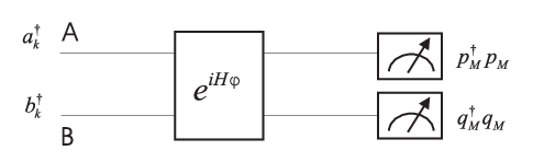
So far we have seen that paired states lead to a gain of a factor of
2 in precision compared to unpaired states in a Ramsey-type
interferometer. This section will show that paired states are even
more powerful and can lead to a precision gain of a factor of
when measuring the phase of a pair-interaction Hamiltonian.
We consider a setup where two fermionic states enter the ports A
and B of an interferometer. The particles entering port A can
occupy the modes , while the particles
entering through port B can occupy the modes
. Then the two states evolve under the
Hamiltonian to be defined below and a particle number
measurement is performed at the end. The situation is depicted in
Fig 4. We will compare the power of paired
states over unpaired ones for two different settings. We start by
introducing some basic notation:
VI.2.1 Prerequisites
We define pair operators and and their equally weighted superpositions
| (58) |
The operators and fulfill the commutation relations
| (59) | |||||
| (60) |
where so that , and
with and being the number operators for particles in
modes and
respectively.
We will compare the power of two paired states and two unpaired
states entering through port A and B. The bound for unpaired
states will be derived again via (43). As and
will be elements of , it is like in the last section
sufficient to compare the power of paired states to those of
sparable states. The paired states will be of the form
| (61) | |||||
with normalization constant , while the separable states are given by
| (63) |
where are separable states in the
modes
and respectively.
After the input state has evolved under the Hamiltonian
into the state an observable is used as
an estimator to determine the parameter to a precision
given by (42). Instead of working in the Schrödinger
picture of state evolution it turns out to be more convenient to
tackle the problem in the Heisenberg picture, where evolves
according to . We are interested in
the phase sensitivity for small , so that we can expand
(42) in powers of , arriving at
| (64) | |||||
If the input state is an eigenvector of with eigenvalue , we obtain the following simple expressions for and
| (65) | |||||
| (66) |
so that the phase fluctuation simplifies to
| (67) |
An observable fulfilling this property is ,
where
The commutation relations for and (59)
imply that in the limit of infinitely many modes the operators and become bosonic. We will thus
start out with a scenario where the input states are in the bosonic
limit and then turn our attention to a setting which is far from the
bosonic limit.
VI.2.2 Bosonic limit
In this section we will consider the scenario , i.e. we are in the bosonic limit, where the limit is taken for the expectation values of the operators. We will consider a coupling of the form where
| (68) |
and measure .
We start deriving the best precision for unpaired states using
(43). We will use a finite for input state,
coupling Hamiltonian and measurement and then take the limit . To be precise, the calculation will be done
for
and . Then due to the conservation of
particle number. Hence, as , where the last inequality results from the bound of the
pairing measure on unpaired states Thm.
V.6. The same holds for . Hence, in the limit the
variance of vanishes. For the setting of paired
states, however, we can obtain the following result:
Theorem VI.4.
For paired input states, the interferometer depicted in Fig 4 allows to estimate the coupling parameter to a precision
| (69) |
Proof.
Consider an interferometric setup depicted in Fig. 4, where the -particle input state and the coupling Hamiltonian are defined in eqs. (61) and (68) respectively. We will again use a finite for input state, coupling Hamiltonian and measurement and then take the limit , i.e. we use and . Making use of the relations
| (70) | |||||
| (71) |
where , a lengthy but straightforward calculation leads to using (67). Taking the limit leads to the result of the theorem. ∎
VI.2.3 Interferometry far from the bosonic limit
In the preceding section we have
studied the power of paired states in the bosonic limit. As the
power of bosonic particles for interferometry has been known for
quite a while, the use of paired states where the fermionic nature
of the particles survives might be a more interesting question. In
this section we will show that even far from the bosonic limit
paired states can achieve a precision gain of
order for quantum metrology.
We will study a coupling Hamiltonian of the form where
| (72) |
First, we will give a bound for the phase sensitivity achievable by using product states at the input:
Theorem VI.5.
Proof.
This bound can be beaten by a factor of using paired states. A lengthy but straightforward calculation leads to the following result:
Theorem VI.6.
This theorem implies for all . In conclusion we have shown that paired states are a resource for quantum metrology. Theorem VI.6 is the main result of this section. We have remarked already at the beginning of this chapter that it has been proven before that the Heisenberg limit can be achieved using fermionic particles [55]. However, these states were constructed in an abstract way, while we prove that the BCS states that can be created easily in an experimental setup are a very powerful resource for quantum metrology.
VII Application to experiments and conclusion
In summary, we have developed a pairing theory for fermionic states. We have given a precise definition of pairing based on a minimal list of natural requirements. We have seen that pairing is not equivalent to entanglement of the whole state nor of its two-particle reduced density operator but represents a different kind of quantum correlation. Within the framework of fermionic Gaussian states we could solve the pairing problem completely. For number conserving states we have given sufficient conditions for the detection of pairing that can be verified by current experimental techniques, e.g. via spatial noise correlations [56, 57, 58] and prescribed a systematic way to construct complete families of pairing witnesses.
To shed some light on the pairing debate [7, 10, 11, 12], we would need access to the proportionality factor linking the quantity plotted in Fig. 4 of [7] to the local pair correlation correlation function .
Another important point of our work is the utility of fermionic states for
quantum metrology. While it has been shown that, in principle, fermionic
states can achieve the Heisenberg limit for precision measurements in a
Ramsey-type interferometer [55], we could prove the
usefulness of states that are available in the laboratory. Furthermore, the
optimal precision for the Ramsey-type setup is proportional to the pairing
measure introduced from an intuitive picture in Secs. II.3
and V. This endows the measure with an
operational meaning.
The results we have presented are just a first step in understanding pairing
and its relation to other types of quantum correlations.
We hope that the pairing theory we have developed will help to get a better understanding of correlated many-body systems, and can provide a new perspective on quantum correlationsa and may serve as a starting point for further inquiries.
For example, one might attempt a finer characterization of pairing, e.g., and represent paired states of rather different nature: it would be interesting to develop witnesses or measures which allow to determine over how many modes the pairs in a given states extend and to relate these differences to applications in metrology ore elsewhere?. Moreover, the theory we developed has been concerned with finitely many modes only and it is an obvious question whether generalizing to an infinite dimensional single-particle space gives rise to new phenomena.
Up to now we have concentrated on fermionic states. But the question of pairing in bosonic systems might be equally interesting and relevant for recent experiments [59].
What about higher-order correlations? The set of unpaired states contains both separable and highly correlated states. This is, for example, reflected in the fact that there are unpaired states which can be transformed to paired ones by single-mode particle number measurements (e.g., by measuring particle number in mode ). A theory of higher-order correlated states could be developed along the lines discussed here, e.g., by changing the set of observables on which the states are compared to uncorrelated ones and defining as th-order correlated those states whose expectation values on th-order observables cannot be reproduced by -correlated states.
Tools and methods from entanglement theory have been very useful in analyzing pairing. One very important such tool, however, is missing: positive maps, that is, transformations which do not correspond to a physical operations but nevertheless, when applied to a subsystem in a separable state with the rest, map density operators to (unnormalized) density operators and thus provides strong necessary conditions for separability. Finding an analogy might prove very useful for the analysis of many-body correlations. Another importat object in the theory of entanglement is the set of LOCC operations (local operations and classical communication), i.e., the operations that cannot create entanglement. In the case of pairing, the analogous set would contain passive operations and discarding modes. Are there other physical transformations that cannot create pairing? Do paired states, then, possibly allow to implement such transformations similar to entanglement enabling non-LOCC operations?
Acknowledgements.
We acknowledge support by the Elite Network of Bavaria QCCC, the DFG within SFB 631, the DFG Cluster of Excellence Munich-Centre for Advanced Photonics, QUANTOP and the Danish Natural Science Research Council (FNU).Appendix A Useful properties of separable states
We give two technical lemmas which involve useful properties of product states.
A.1 Bound of on separable states
In this section we prove a bound of a some special two-body operator on product states:
Lemma A.1.
Let be a separable state. Then
| (74) |
Proof.
Let be the Hilbert space spanned by and define . Then , where is a mixed separable state according to Lemma II.2, and denotes the occupation number basis for the subspace . It is easily checked that can have non-vanishing expectation value only for the two-particle state Using for any complex numbers and the normalization conditions , one arrives at . ∎
A.2 Expectation values of one-and two-body operators for separable states
In this section we will prove that the one-and two-body operators for separable states can be expressed in terms of matrix elements of projectors.
Lemma A.2.
Let be a pure separable state. Then
| (75) | |||||
where is a projector of rank .
Proof.
Consider modes. We go into the basis where the pure separable state is of the form In this basis , i.e. for , where . Now let . Then
and is a projector of rank .
For the one-particle operators, we obtain as .
∎
Appendix B Proof of Lemmas V.1 and V.2
B.1 Proof of Lemma V.1
Proof.
As are built up
of operators that are the product of at most two creation and
annihilation operators, we can prove the lemma for separable
states. In the first step, we will show that the three operators
are positive on all separable states. Then we will show that all
states within the set bounded by correspond to a separable state. Finally we will
show there exist states that are detected as paired by
and . Positivity of
on all number conserving states will be shown in
the proof of Lemma V.1 following below.
To show positivity of it is sufficient to show the positivity for pure
separable states, as the result for mixed states follows from
convexity. From now on, let
In Lemma A.2 (see appendix A) we have
shown that the expectation values of number conserving one-and
two-body operators can be expressed in terms of matrix elements of
projectors. Let be the rank projector such that , and let the
principal submatrix of where the indices run over Then we have the following inequalities:
| (77) | |||||
| (79) | |||||
These results imply
| (80) |
We use the inclusion principle [43], stating that the eigenvalues of a principal submatrix of a Hermitian matrix fulfill where the eigenvalues are arranged in increasing order. As is a projector, we have . Hence,
| (81) |
Define , . Then
and as we
conclude that .
We will need the lemma II.2:
where ,
and are separable -particle states. Let
Then a straightforward calculation leads to , ,
and . Linearity of the trace implies
Hence, all separable states lie within the set bounded by the
planes defined by the witness operators
Next, we show that each point within the polytope
corresponds to a separable state. As
is convex, it is sufficient to check that for every
extreme point of there exists a separable
state. This is indeed the case: The extreme points of
are , , ,
which correspond for example to the separable
states , , and
respectively.
It remains to show that and are
pairing witnesses. Define Then
.
∎
B.2 Proof of Lemma V.2
Proof.
It is sufficient to prove the lemma for , as the result for a general number
conserving state follows from convexity.
Shown in the proof of Thm. V.2.
Let be the reduced
density operator in the modes We can rewrite
in the form Defining we obtain . This implies
As in the proof of Lemma V.1 it remains to show that
the extreme points of correspond to some
fermionic state. It has been shown in the proof of Lemma
V.1 that , and can be
reached by some separable state. The remaining two extreme points,
correspond for example to the state
.
∎
Appendix C Proof of Thm. V.4
In this section we will provide all the details leading to Thm. V.4, starting with the bound on separable states:
Lemma C.1.
Let with and let be as in Thm. V.4. Then .
Proof.
The operator acts non-trivially only on the modes . Denote by the reduced density operator obtained when tracing out all but these four modes. According to Lemma II.2, is a convex combination of separable -particle states . We proved in Lemma A.1 that . Hence . Now and so that . Due to the particle number constraint this value can be taken for . Hence, so that . ∎
To show the witness character of we also have to prove that there exists a BCS state that is detected by the Hamiltonian. We will need the following theorem about the distribution described by the in (20):
Theorem C.2.
Proof.
For the proof we will need a theorem from probability theory known as Lyapunov’s central limit theorem [60]:
Theorem C.3.
(Lyapunov’s central limit theorem)
Let be independent random variables with
distribution functions , respectively, such that and , with
at least one . Let and
If the Lyapunov condition
is satisfied for some then the normalized partial sums converge in distribution to a random variable with normal distribution
Consider the observables , where is the number of particles with quantum numbers respectively. The can be considered as classical random variables since they commute mutually. In the variational BCS-state the random variable is distributed according to the probability distribution
| (83) | |||||
| (84) | |||||
With the help of Thm. C.3 applied to the random variable we can now complete the proof of Thm. C.2, i.e. show that converges to a normal distribution for large . We start calculating the expectation value of . For a BCS-state, , as particles with quantum numbers always appear in pairs. As , we get and . For calculating the variance, note that , and . Hence
| (85) |
To apply the central limit theorem, we consider . Using , , and we arrive at
| (86) | |||||
Setting in the Lyapunov condition, we obtain
| (87) |
where we have applied the assumption of the theorem in the last step. The central limit theorem implies that converges to a normal distribution with expectation values and variance . ∎
With this result at hand we can prove the following:
Lemma C.4.
Let and be defined as in Thm. V.4. If , then
Proof.
We will use the correspondence of variational and number
conserving BCS states, deriving first a bound for , where
with
like in Thm. V.4. To do so, we will need that the
are normally distributed. From where
and , it follows that . Hence, we know from Thm.
C.2 that the describe a normal
distribution around with standard deviation .
Now, write ,
where
We start with a bound for , where
A bound for can be easily derived noting that
| (89) |
and for we have as . Hence,
| (90) | |||||
where we have approximated the sum by an integral in the second step. For bounding , we will show first that for where we have . Expanding the BCS wave function
| (91) |
the expectation value of the number operator is easily calculated to be , where
| (92) |
If , there exists a lower bound on the coefficients . Then and are related via
In the proof of Thm. C.2 we show that
| (93) |
resulting in
For and the normal distribution of the implies . Hence, . For , this is equivalent to , which can be achieved for . The last condition is satisfied, as we are considering dilute systems, where . Thus, , implying , as . Using (89) and a telescope sum, we conclude that
| (95) | |||||
Next, we derive the bound for the operator . Its expectation value is given by
| (96) |
For , we use the same argumentation we have used for bounding , to obtain
| (97) |
Further, due to the symmetry . Hence, . Thus, up to a factor of 2 we obtain the same bound as for . Putting all the pieces together we find that
In the limit of large , the error function can be approximated by the following formula:
| (99) |
As , we conclude
for . A straightforward calculation results in , leading immediately to the statement of the theorem. ∎
Appendix D Lemma for the proof of Thm. V.6
Lemma D.1.
Every pure separable state fulfills , and this bound is tight.
Proof.
Using Lemma A.2, we obtain
| (100) |
where and . Using the triangle-inequality we get
In the last step we have used the property that the sum of the
squares of a normal matrix is equal to the sum of squares of its
eigenvalues. Taking the square root we obtain
the bound of our claim.
The bound is tight, as implies
which is obtained for
.
∎
Appendix E Proof of Lemma III.5
Proof.
Let and consider the subspace spanned by the states In this basis, the two-particle RDO of is of the form
| (101) |
where . The witness operator
of Thm. V.1 has a negative expectation
value on , hence the state is paired in these modes.
For solving the entanglement question we will use the following
theorem [25] applicable to mixed fermionic
states of two particles each living on a single-particle Hilbert
space of dimension four:
Theorem E.1.
Let the mixed state acting on have a spectral decomposition where is the rank of , and the eigenvectors belonging to nonzero eigenvalues are normalized as Let in some basis, and define the complex symmetric matrix by
| (102) |
which can be represented using a unitary matrix as with diagonal and The state has Slater number 1 if and only if
| (103) |
The spectral decomposition of is given by
where , and . Here and . Defining one obtains
| (104) |
with spectrum . For the state is separable, so we can take . Hence, is the eigenvalue with biggest absolute value. According to Thm. E.1, the reduced state in the subspace of the four modes is entangled iff . For our example, this holds iff . ∎
References
- [1] J. Bardeen, L. N. Cooper, and J. R. Schrieffer, Phys. Rev. 108, 1175 (1957).
- [2] M. Greiner, C. Regal, and D. Jin, Nature 426, 537 (2003).
- [3] S. Jochim, M. Bartenstein, A. Altmeyer, G. Hendl, S. Riedl, C. Chin, J. H. Denschlag, and R. Grimm, Science 302, 2101 (2003).
- [4] M. W. Zwierlein, C. A. Stan, C. H. Schunck, S. M. F. Raupach, S. Gupta, Z. Hadzibabic, and W. Ketterle, Phys. Rev. Lett. 91, 250401 (2003).
- [5] M. Zwierlein, J. Abo-Shaeer, A. Schirotzek, C. Schunck, and W. Ketterle, Nature 435, 1047 (2005a).
- [6] M. Zwierlein, C. Schunck, A. Schirotzek, and W. Ketterle, Nature 442, 154 (2005b).
- [7] G. B. Partridge, K. E. Strecker, R. I. Kamar, M. W. Jack, and R. G. Hulet, Physical Review Letters 95, 020404 (pages 4) (2005).
- [8] M. W. Zwierlein, C. A. Stan, C. H. Schunck, S. M. F. Raupach, A. J. Kerman, and W. Ketterle, Physical Review Letters 92, 120403 (pages 4) (2004).
- [9] C. A. Regal, M. Greiner, and D. S. Jin, Physical Review Letters 92, 040403 (pages 4) (2004).
- [10] G. B. Partridge, W. Li, R. I. Kamar, Y. Liao, and R. G. Hulet, Science 27, 120403 (2006a).
- [11] M. W. Zwierlein and W. Ketterle, Science 314, 54a (2006).
- [12] G. B. Partridge, W. Li, R. I. Kamar, Y. Liao, and R. G. Hulet, Science 314, 54b (2006b).
- [13] C. Schunck, Y. Shin, A. Schirotzek, M. Zwierlein, and W. Ketterle, Science 316, 867 (2007).
- [14] P. Zanardi, Phys. Rev. A 65, 042101 (2002).
- [15] P. Zanardi and X. Wang, J. Phys. A:Math. Gen. 35, 7947 (2002).
- [16] D. Larsson and H. Johannesson, Physical Review A (Atomic, Molecular, and Optical Physics) 73, 042320 (pages 4) (2006).
- [17] M. M. Wolf, Physical Review Letters 96, 010404 (pages 4) (2006).
- [18] D. Gioev and I. Klich, Physical Review Letters 96, 100503 (pages 4) (2006).
- [19] M. Cramer, J. Eisert, and M. B. Plenio, Physical Review Letters 98, 220603 (pages 4) (2007).
- [20] Y. Shi, Phys. Rev. A 67, 024301 (2003).
- [21] R. Paškauskas and L. You, Phys. Rev. A 64, 042310 (2001).
- [22] M.-C. Banuls, J. I. Cirac, and M. M. Wolf, Physical Review A (Atomic, Molecular, and Optical Physics) 76, 022311 (pages 13) (2007).
- [23] H. M. Wiseman and J. A. Vaccaro, Phys. Rev. Lett. 91, 097902 (2003).
- [24] J. Schliemann, J. I. Cirac, M. Kuś, M. Lewenstein, and D. Loss, Phys. Rev. A 64, 022303 (2001a).
- [25] K. Eckert, J. Schliemann, D. Bruss, and M. Lewenstein, Annals of Physics 299, 88 (2002).
- [26] M. R. Dowling, A. C. Doherty, and H. M. Wiseman, Physical Review A (Atomic, Molecular, and Optical Physics) 73, 052323 (pages 12) (2006).
- [27] J. Schliemann, D. Loss, and A. H. MacDonald, Phys. Rev. B 63, 085311 (2001b).
- [28] N. Schuch, F. Verstraete, and J. I. Cirac, Phys. Rev. A 70, 042310 (2004a).
- [29] N. Schuch, F. Verstraete, and J. I. Cirac, Phys. Rev. Lett. 92, 087904 (2004b).
- [30] S. Bravyi, Quantum Inf. and Comp. 5, 216 (2005).
- [31] G. D. Mahan, Many-Particle Physics (Kluwer Academic, 2000), 3rd ed.
- [32] L. Amico, R. Fazio, A. Osterloh, and V. Vedral, Rev. Mod. Phys. 80, 517 (pages 60) (2008), URL http://link.aps.org/abstract/RMP/v80/p517.
- [33] V. Bach, E. Lieb, and J. Solovej, Journal of Statistical Physics 76, 3 (1994).
- [34] C. Bloch and A. Messiah, Nuclear Physics 39, 95 (1962).
- [35] A. Coleman and V. Yukalov, Reduced Density Matrices (Springer-Verlag, 2000).
- [36] M. Horodecki, P. Horodecki, and R. Horodecki, Phys. Lett. A 223, 1 (1996), eprint quant-ph/9605038.
- [37] W. Rudin, Functional Analysis (McGraw-Hill, 1991), 2nd ed.
- [38] R. Rockafellar, Convex Analysis (Princeton University Press, 1970).
- [39] P. W. Anderson, Phys. Rev. 112, 1900 (1958).
- [40] R. A. Barankov and L. S. Levitov, Phys. Rev. Lett. 93, 130403 (2004).
- [41] R. A. Bertlmann, K. Durstberger, B. C. Hiesmayr, and P. Krammer, Physical Review A (Atomic, Molecular, and Optical Physics) 72, 052331 (pages 9) (2005), URL http://link.aps.org/abstract/PRA/v72/e052331.
- [42] A. Leggett, Modern Trends in the Theory of Condensed Matter (A. Pekalsky, R. Przystawa (Springer-Verlag, Berlin), 1980).
- [43] R. Horn and C. Johnson, Matrix Analysis (Cambridge University Press, 1985).
- [44] D. J. Wineland, J. J. Bollinger, W. M. Itano, and D. J. Heinzen, Phys. Rev. A 50, 67 (1994).
- [45] J. J. Bollinger, W. M. Itano, D. J. Wineland, and D. J. Heinzen, Phys. Rev. A 54, R4649 (1996).
- [46] S. L. Braunstein and C. M. Caves, Phys. Rev. Lett. 72, 3439 (1994).
- [47] S. L. Braunstein, C. M. Caves, and G. Milburn, Annals of Physics 247, 135 (1996).
- [48] K. Eckert, P. Hyllus, D. Bruss, U. V. Poulsen, M. Lewenstein, C. Jentsch, T. Muller, E. M. Rasel, and W. Ertmer, Physical Review A (Atomic, Molecular, and Optical Physics) 73, 013814 (pages 10) (2006).
- [49] B. Yurke, S. L. McCall, and J. R. Klauder, Phys. Rev. A 33, 4033 (1986).
- [50] M. J. Holland and K. Burnett, Phys. Rev. Lett. 71, 1355 (1993).
- [51] P. Bouyer and M. A. Kasevich, Phys. Rev. A 56, R1083 (1997).
- [52] C. C. Gerry, Phys. Rev. A 61, 043811 (2000).
- [53] W. J. Munro, K. Nemoto, G. J. Milburn, and S. L. Braunstein, Phys. Rev. A 66, 023819 (2002).
- [54] S. F. Huelga, C. Macchiavello, T. Pellizzari, A. K. Ekert, M. B. Plenio, and J. I. Cirac, Phys. Rev. Lett. 79, 3865 (1997).
- [55] B. Yurke, Phys. Rev. Lett. 56, 1515 (1986).
- [56] E. Altman, E. Demler, and M. D. Lukin, Phys. Rev. A 70, 013603 (2004).
- [57] T. Rom, T. Best, D. van Oosten, U. Schneider, S. Foelling, B. Paredes, and I. Bloch, Nature 444, 733 (2006).
- [58] M. Greiner, C. A. Regal, J. T. Stewart, and D. S. Jin, Physical Review Letters 94, 110401 (pages 4) (2005).
- [59] S. Riedl, E. R. S. Guajardo, C. Kohstall, A. Altmeyer, M. J. Wright, J. H. Denschlag, R. Grimm, G. M. Bruun, and H. Smith (2008), eprint arXiv:0809.1814v1 [cond-mat.other].
- [60] P. Billingsley, Probability and Measure (Wiley-Interscience, 1995), 3rd ed.