UCLA/08/TEP/29
CPHT-RR079.1008
23 October 2008
Exact Half-BPS Flux Solutions in M-theory II:
Global solutions asymptotic to 22
2
This work was supported in
part by NSF grants PHY-04-56200 and PHY-07-57702.
E-mail addresses:
dhoker@physics.ucla.edu; johnaldonestes@gmail.com; gutperle@physics.ucla.edu;
dk320@physics.ucla.edu.
Eric D’Hokera, John Estesb, Michael Gutperlea and Darya Kryma
Department of Physics and Astronomy
University of California, Los Angeles, CA 90095, USA
Centre de Physique Th«eorique, Ecole Polytechnique,
FÐ91128 Palaiseau, France
Abstract
General local half-BPS solutions in M-theory, which have symmetry and are asymptotic to , were constructed in exact form by the authors in [arXiv:0806.0605]. In the present paper, suitable regularity conditions are imposed on these local solutions, and corresponding globally well-defined solutions are explicitly constructed. The physical properties of these solutions are analyzed, and interpreted in terms of the gravity duals to extended 1+1-dimensional half-BPS defects in the 6-dimensional CFT with maximal supersymmetry.
1 Introduction
One realization of the AdS/CFT correspondence [2, 3, 4] in M-theory is the duality of the vacuum and the 6-dimensional CFT which is obtained by a decoupling limit of the M5 brane world-volume theory [5, 6, 7]. The nonabelian world-volume theory of multiple M5-branes is presently unknown and the 6-dimensional CFT has been formulated in the light cone gauge [8]. One interesting class of deformations in this theory is given by the insertion of local half-BPS chiral operators, where half-BPS means the operators preserve sixteen of the thirty-two supersymmetries. The gravitational duals of these operators are the half-BPS solutions of Lin, Lunin, and Maldacena [9].
In our recent paper [10] (see also [11, 12, 13, 14] for earlier work), new exact solutions of 11-dimensional supergravity were constructed which preserve sixteen of the thirty-two supersymmetries. In addition, the solutions preserve a bosonic symmetry. Correspondingly, the 11-dimensional metric is constructed as a warped product of over a 2-dimensional base space . These solutions can be interpreted as the gravity duals of extended supersymmetric defects in the CFT. The solutions are local in the sense that for a bosonic background, the vanishing of gravitino variation as well as the bosonic equations of motion and Bianchi identities are satisfied point wise, except at possible singularities.
In general, the local solutions of [10] contain a large variety of solutions many of which contain singularities. An important problem is to pick out solutions which are asymptotic to either or and everywhere regular so that the supergravity approximation is valid. In particular this requires one to examine the global structure of the solutions. Similar analysis have been carried out in Type IIB supergravity in [9, 16, 19]. An amazing result in all cases is that the regularity conditions in addition to the general local solution admit a superposition principle for the half-BPS objects in the theory. We expect such a principle to emerge from the analysis here. There are two distinct classes of solutions which were found in [10]:
Case I contains solutions asymptotic to . The superalgebra of symmetries is . The super Lie algebra is a particular real form of . In the classification of [18] this solution is case IV of table 11. M-theory on is dual to a 3-dimensional CFT which is obtained by a decoupling limit of the world-volume theory of M2 branes. The local BPS solution is dual to -dimensional conformal defects in the 3-dimensional CFT, analogous to the half-BPS defect solutions obtained in type IIB string theory [15, 16] (see also [17] for earlier work).
Case II contains solutions asymptotic to . The bosonic isometries together with the supersymmetries form a superalgebra which is given by . The supergroup is a different real form of than the one appearing in case I. In the classification of [18] this solution is case VII of table 12. M-theory on is dual to a 6-dimensional CFT which is obtained by a decoupling limit of the world-volume theory of M5 branes. The local BPS solution is dual to -dimensional conformal defects in the 6-dimensional CFT, analogous to the half-BPS Wilson loop solutions obtained in type IIB string theory [19] (see also [13, 20] for earlier work).
The local solutions presented in [10] are very similar for the case I and II as the underlying integrable system is the same. However, the analysis of the regularity and the global structure is quite different. In this paper we will focus on the solution of case II. The analysis of the regularity and global structure for case I will be analyzed in a separate paper [21].
The structure of the paper is as follows. In section 2 the features of the local solution for case II which are important for the present paper will be reviewed. In section 3 the boundary conditions on the solution implied by regularity are analyzed. A general solution which satisfies suitable boundary condition is constructed and it is shown that the solution is regular everywhere. In section 4 the global structure of the solutions as well as its interpretation in terms of the dual 6-dimensional conformal field theory is discussed. In appendix A detailed proof of the regularity of our solution is presented.
2 Summary of local solution
In this section we review the local half-BPS solution of [10]. Derivations and more calculational details can be found in that paper. The 11-dimensional metric is a fibration of over a 2-dimensional Riemann surface ,
| (2.1) |
The four form field strength is given by
| (2.2) |
Here and are the volume forms on and respectively. In addition is the vielbein on . It is always possible to choose local complex coordinates on the Riemann surface such that the 2-dimensional metric in (2.1) is given by
| (2.3) |
The metric factors , as well as the flux fields , and only depend on .
The Ansatz respects symmetry which can be interpreted as the symmetries of a 1+1-dimensional conformal defect in the 6-dimensional M5 brane CFT. The condition that 16 supersymmetries are unbroken is equivalent, for a purely bosonic background, to the statement that the gravitino supersymmetry variation vanishes for 16 linearly independent supersymmetry variation parameters.
In [10] the BPS conditions were solved, and it was shown that the half-BPS solution is completely determined by the choice of a 2-dimensional Riemann surface , a real harmonic functions on and a complex function which is a solution of the following linear equation,
| (2.4) |
In order to express the local half-BPS solution in terms of and it is useful to define the following quantity
| (2.5) |
The metric factors in (2.1) are then given by
| (2.6) |
The metric factor in (2.3) is given by
| (2.7) |
The fluxes are defined by conserved currents as follows
| (2.8) |
where the conserved currents can be expressed in a compact way by defining
| (2.9) |
and are given by
| (2.10) |
It was shown in [10] that the equations of motion of as well as the Bianchi identities are satisfied for a harmonic and a which solves (2.4).
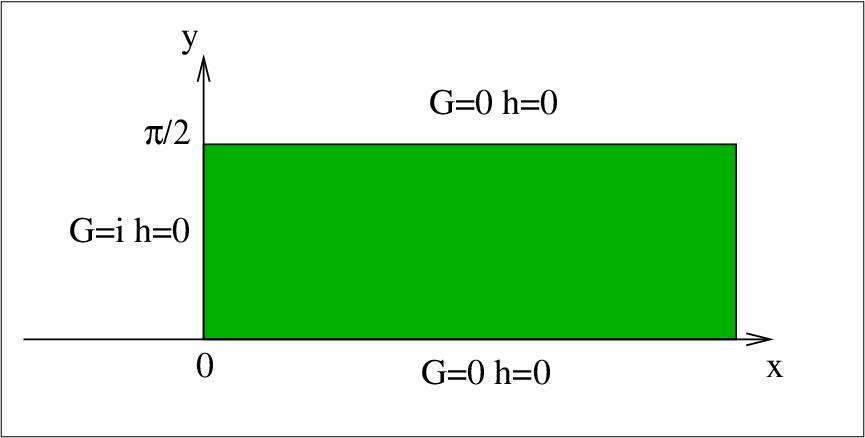
The simplest solution is the maximally symmetric itself. The Riemann surface is the half strip . Denoting the holomorphic coordinate as , the functions and are given by
| (2.11) |
Plugging this into (2.6) the metric factors become
| (2.12) |
Note that the Riemann surface has three boundary components. The boundary is characterized by the vanishing of the harmonic function . Furthermore, taking or , we find , while taking , we find . So takes the values and on the boundary of . The boundary of on the other hand is located at .
3 Regularity
In this section, we analyze the regularity conditions and the global structure of the solution. We look for solutions which are everywhere regular and which are asymptotic to . This leads to the following three assumptions for the geometry.
- 1.
The boundary of the 11-dimensional geometry is asymptotic to .
- 2.
The metric factors are finite everywhere, except at points where the geometry becomes asymptotically , in which case the metric factor and one of the sphere metric factors diverge.
- 3.
The metric factors are everywhere non-vanishing, except on the boundary of , in which case at least one sphere metric factors vanishes. In addition, both sphere metric factors may vanish only at isolated points.
The second requirement guarantees that all singularities in the geometry are of the same type as . The third requirement guarantees that the boundary of corresponds to an interior line in the 11-dimensional geometry.
It follows from (2.6) that a particular combination of metric factors is very simple
| (3.1) |
The metric factor is positive definite and cannot vanish [10]. Hence the condition (which defines a 1-dimensional subspace in ) occurs if and only if at least one of the metric factors for the spheres or vanishes. It follows from assumption , that defines the boundary of .
Note that the equation for (2.4) is covariant under conformal reparamaterizations. This freedom allows one to choose local conformal coordinates11 1 We use a slightly different notation: the coordinate in this paper was called in [10].
| (3.2) |
Here, is the harmonic function dual to so that is holomorphic, i.e. . The domain of the new conformal coordinate is the right half plane and the boundary of is at , i.e. the vertical axis.
In the coordinates , it is useful to decompose into its real and imaginary parts,
| (3.3) |
for real functions. The real and imaginary parts of equation (2.4) are respectively,
| (3.4) | |||||
| (3.5) |
Equation (3.5) can be solved in terms of a single real potential
| (3.6) |
Equation (3.4) becomes a second order partial differential equation on ,
| (3.7) |
The general local solution of (3.7) can be obtained by a Fourier transformation with respect to , which produces an ordinary differential equation which can be solved by [10]
| (3.8) |
Here is the modified Bessel function of the second kind. There is a second linearly independent solution of the form (3.8) which involves the modified Bessel function of the first kind . However this solution has the wrong behavior for large and fails to obey the regularity condition . In [10] an explicit expression for and was found by defining
| (3.9) |
and using the following integral representation of
| (3.10) |
Using (3.8)- (3.10) can be expressed in terms of
| (3.11) |
and (3.6) can be used to write as follows
| (3.12) |
3.1 Boundary conditions on
In this section we analyze the boundary conditions has to satisfy at or in the coordinates at in order for the solution to be regular near the boundary. It will be useful to have the following expressions for the metric factors obtainable from (2.6)
| (3.13) |
The behavior near the boundary (the regularity in the bulk of will be discussed in the next section) is exhibited by expanding , at fixed , in a power series in ,
| (3.14) |
where the are all functions of . Note that the reality of the solution implies that is bounded and hence no negative powers of can appear in the series expansion (3.14). Equation (3.4) and (3.5) impose the vanishing of even/odd powers of in respectively. Furthermore these equations impose differential equations in between the different but these relations will not be needed in the following. The following power series expansions will be useful in the following analysis,
| (3.15) |
When , we have as . From (3.13), the product goes to zero as and the geometry will be singular unless . It follows from (3.15) that one has to choose in order to avoid a singularity. If this is the case, will remain finite, while so that the volume of the sphere tends to zero. Comparing with the solution, this behavior is associated with the boundary component of (2.11).
When , we will have while will remain finite, as long as the conditions and are satisfied. If this is the case, the volume of the sphere will tend to zero. Comparing with the solution, this behavior is associated with the boundary component of (2.11).
In summary we have the following boundary conditions on G and the metric factors
| (3.16) |
3.2 General regular solution
We first parameterize the boundary conditions for at which leads to solutions satisfying regularity conditions 1 to 3, listed at the beginning of section 3. As we shall see, a further condition needs to be imposed to guarantee the absence of singularities in the bulk, namely the values of in the second line of (3.16) will be restricted to be either all positive or all negative.
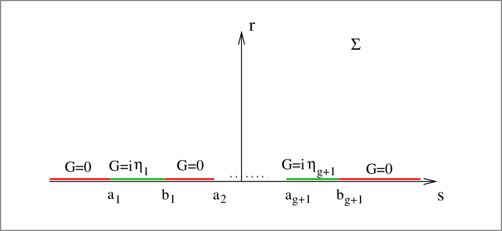
General boundary conditions for are given by the choice of points on the axis,
| (3.17) |
The solution corresponds to . There are two kinds of intervals which are distinguished by the boundary condition for .
| (3.18) |
where . The boundary conditions can be implemented as follows:
| (3.19) |
where is the step function. Since on each segment, can take only the values , no two bumps can “overlap”, and this forces the and to alternate as in (3.17).
It remains to calculate from the boundary condition in (3.19). To this end, we first take the Fourier transform in with , of (3.6) with (3.8) plugged in
| (3.20) |
whose limit is simply obtained using the asymptotics of , and we find,
| (3.21) |
Using the boundary condition of (3.19), we thus have
| (3.22) |
The Fourier transform can be done exactly
| (3.23) |
The expression for may then be obtained using the integral representation (3.12)
| (3.24) |
After some simplifications, we obtain,
| (3.25) |
where the quantities and are defined as
| (3.26) |
are both real. Next we use the integral formula
| (3.27) |
The result is an algebraic expression for which solves (3.4) and satisfies the boundary condition (3.19) and is given by
| (3.28) |
It is easy to see that (3.28) is equal to (3.19) in the limit .
3.3 Regularity in the bulk
In the remainder of this section we give an argument that the general solution (3.28) is regular everywhere. Note that the general solution was constructed in section 3.2 by demanding that the geometry is regular at the boundary of .
The general solution (3.28) should also approach the boundary asymptotically as . The expression for . given in (2.11) can be recovered from the general regular solution (3.28) by setting , , and .
| (3.29) | |||||
where we have used the coordinates and . The boundary of is reached by taking . Using the same coordinate change for the general solution it is easy to see that (3.28) approaches in the limit .
It remains to show that the geometry is regular in the interior for . Since in the chosen coordinate system the regularity of the solution requires that away from the boundary is required to satisfy the strict inequality . Note that this condition automatically guarantees that we also have . Furthermore the relation
| (3.30) |
shows that if then individually and . Examining the explicit formula for the metric factors (2.6) one can see that they are then finite and the geometry is thus regular. It is shown in Appendix A if the obey the ordering (3.17) and the are all either or , that in the upper half plane and hence the solution is regular everywhere.
To see the converse, that is if in the bulk then the solutions is singular, we first note that for to vanish, either or must vanish. Taking the ratio of and in (2.6) we see that one of them must either be vanishing or be infinite resulting in a singular geometry.
3.4 The solution
In this section, we examine the solution in detail, specifically we choose the parameters for the general solution (3.28) as follows:
| (3.31) |
In Figure 3, we show the behavior of the metric factors. The sphere metric factors alternatingly vanish as . While as , the metric factors flatten out to those of .

For there are singularities as we approach , but these are coordinate singularities and are due to the conformal transformation we made in order to map the half-strip to the upper half plane.

An important feature of the solutions with is that there are additional nontrivial four cycles in the geometry. We can illustrate this feature for the solution (3.31). In addition to the four cycle which is already present in the solution, there are two additional nontrivial four cycles and .
The behavior of the fluxes for the solution is very interesting. For comparison purposes we first plot the fluxes (2.8) for the solution given by (3.28) with
| (3.32) |

Note that the fluxes and vanish identically and the only nontrivial flux is . There is only one nontrivial topological cycle forming a four sphere. The integrated flux is nothing but the non-vanishing four form flux through the four sphere in .

In Figure 6, we plot the fluxes for the solution (3.31). Due to the complicated form of the currents (2.8) we have not been able to integrate them to analytically obtain a closed form of the fluxes. However it is clear from figure 6 that the solution has indeed nontrivial flux through the cycles and for and respectively.
4 Discussion
In the previous section we found a family of regular half-BPS solutions labelled by an integer and real moduli. In this section we discuss the interpretation of these solutions from the point of view of the AdS/CFT correspondence. The spacetime is obtained as the near horizon limit of a large number of M5 branes. The AdS/CFT duality relates M-theory on this background to the decoupling limit of the M5-brane world-volume theory which defines a 6-dimensional CFT with supersymmetry [6, 5].
A first step towards interpreting the solution is to understand the boundary structure. The only region on where the spacetime becomes asymptotically is . There is however another boundary component since the factor also has a boundary. This can be seen by rewriting the metric (2.1).
| (4.1) |
The boundary of is reached as and the boundary metric is obtained by stripping off the (divergent) conformal factor . The factor in front of the metric factors of the spheres and implies that the boundary in the limit is -dimensional space extending in the plane. The isometry of the factor corresponds to the conformal symmetry of the -dimensional defect, which is contained in the supergroup of preserved superconformal symmetries. Note that for all values of and the moduli there is only one defect.
The interpretation of the 1+1-dimensional half-BPS defect from the perspective of the dual CFT is the supersymmetric self dual string solution of the 6-dimensional supersymmetric M5-brane world-volume theory [22, 23, 24] which was constructed in [25]. The selfdual string in the theory can also be interpreted as the boundary of an open M2 brane which ends on the M5-brane [26, 27] Unfortunately the action for multiple membranes is not well understood and the selfdual string soliton solution has only been derived for the abelian case of a single 5-brane.
There is a strong analogy of the selfdual string defect with the BPS-Wilson loop in Type IIB string theory. While the details of the supergravity solution are somewhat different the general structure of the half-BPS flux solution and its moduli space presented in section 3.2 is intriguingly similar to the Type IIB supergravity flux solutions dual to BPS Wilson loops which was found in [19].
The BPS Wilson loop in also has a probe description. The original proposal [36, 37] identified the Wilson loop in the fundamental representation with a fundamental string with world-volume inside . BPS-Wilson loops in higher rank symmetric representation and are identified with a probe D3 brane with electric flux with world-volume inside . BPS-Wilson loops in higher rank anti-symmetric representation and are identified with a probe D5 brane with electric flux with world-volume inside [28, 29].
The 1+1-dimensional BPS defect in the 6-dimensional CFT can be viewed as the insertion “Wilson surface”-operator [30, 31, 32, 33]. In the probe approximation one can use a analogy between the Wilson loop in SYM and the Wilson surface operators: The fundamental string is related to M2-brane probe. The D3 brane with electric flux and world-volume is related to a probe M5 brane with 3-form flux on its world-volume (with the embedded in the ). The D5 brane with electric flux and world-volume is related to a probe M5 brane with three form flux on its world-volume (with the embedded in the ). These probe branes and their supersymmetry where analyzed in [34, 35, 14]
The supergravity solutions we have obtained are the analog of the “bubbling” Wilson loop solutions [19, 13, 29]. They are fully backreacted and replace the probe branes by geometry and flux. In particular as the discussion of the solution in section 3.4 showed there are two new nontrivial four cycles in the solution. The fluxes through these cycles are the remnants of the probe M5-branes in the backreacted solution.
Unfortunately the theory for multiple M5-branes is not as well understood as SYM theory. It is possible that the bubbling solutions can be useful in the understanding of the M5-brane theory. It would be interesting to see whether there is an analog of the matrix model description of the BPS-Wilson loops (and its relation to the bubbling supergravity solution) for the Wilson surfaces.
The general solution we have obtained has only one asymptotic region. It would be interesting to investigate whether its possible to have more than one asymptotic region, this would presumably correspond to a harmonic function with multiple poles. A similar phenomenon occurs in the case of half-BPS solutions which are asymptotic to which we are currently investigating [21].
Acknowledgments
MG gratefully acknowledges the hospitality of the International Center for Theoretical Science at the Tata Institute, Mumbai and the Department of Physics and Astronomy, Johns Hopkins University during the course of this work.
Appendix A Proof of the regularity condition
In this appendix we shall prove a theorem which is central to establishing the regularity of the general solution constructed in section 3.2.
Theorem 1 When all are equal to one another, the function , defined by
| (A.1) |
satisfies , for all subject to the ordering condition
| (A.2) |
Numerical analysis suggests that this property holds, and also shows that, when not all are equal to one another, the condition is violated for some range of and . We shall prove Theorem 1 for for all ; the theorem for the opposite case then follows immediately.
We begin by simplifying the condition as follows,
| (A.3) |
The second factor on the right hand side of the last equality is manifestly positive for all , and may be dropped in the inequality. Thus, the condition becomes equivalent to the condition , which is equivalent to the following quadratic inequality
| (A.4) |
where are real. In the sequel, it will be convenient to introduce the following notations,
| (A.5) |
In terms of these functions, we define the following partial sums, for ,
| (A.6) |
so that the real and imaginary parts of , defined in (A.4), are given by .
The first key ingredient in the proof of Theorem 1 will be the fact that, for , the functions and are strictly monotonically increasing as increases.
A.1 The case
We begin by proving Theorem 1 for the following special ordering,
| (A.7) |
Using the fact that and are monotonically increasing with for , it is immediate that and . Both bounds are sharp, as they can be saturated at the boundary of the domain (A.2) in the limit where . A lower bound for and an upper bound for may be obtained by letting (with ). Putting all together, we obtain the following double-sided bounds,
| (A.8) |
To prove , we proceed recursively. Using the definition (A.6), we have,
| (A.9) |
where we use the abbreviations , and . Notice that we have and . The quantity of interest is
| (A.10) |
Here, we have suppressed the absolute value sign on , as we already know that . To show that holds, it will suffice to show that . Thus, we need to derive an optimal upper bound for , and show that this bound is less than .
We first derive an upper bound on as a function of and , subject to the condition that . To this end, express as follows,
| (A.11) |
The bounds established earlier, namely and , guarantee that and for all values of . We now search for the maximum of as a function of over the interval , with viewed as fixed. To determine it, we investigate the derivative with respect to ,
| (A.12) |
This derivative can vanish in the interval if and only if . If this is the case, the corresponding point is , which should satisfy .
Hence, the extrema of as a function of may be attained either at , or at either one of the extremities of the interval . These three values are given by,
| (A.13) |
Since , it is manifest that . Thus, cannot be the optimal upper bound for . Comparing the remaining two possible values, we find,
| (A.14) |
Given that and , it follows that the right hand side is positive and so that is the optimal upper bound. In summary,
| (A.15) |
for all values of such that .
Since and , it is straightforward to derive an upper bound for the right hand side of (A.15). Indeed, both terms increase as decreases. Thus, the optimal bound for the right hand side is attained when assumes its smallest possible value, which is . Hence, we have
| (A.16) |
But, using the definitions of and in terms of and , we see that the quantity admits a drastic simplification,
| (A.17) |
Combining all, we get a recursive series of bounds,
| (A.18) |
From their definitions, , we readily find , so that . This concludes the demonstration of Theorem 1 for the case .
A.2 The case
Next, we proceed to proving Theorem 1 for the following special ordering,
| (A.19) |
It is not necessary to repeat the steps analogous to the proof for the case , since we can reduce the present case to the case by changing variables,
| (A.20) |
The and are now all positive and satisfy the following ordering,
| (A.21) |
Denoting the corresponding function by , and its real and imaginary parts by and , we have by definition,
| (A.22) |
where and are given by (A.6) but with and . From the proof of the case , it now follows that also for this special case.
A.3 The general case
Next, we shall prove Theorem 1 for the cases whose ordering is given by
| (A.23) |
for . (The proof for the case with the ordering follows the same steps, or may be derived by taking the limit in the ordering of (A.23), and need not be detailed here.)
It remains only to prove Theorem 1 for the ordering (A.23). To do so, we use the fact that the behaviors of the variables larger than 0 and those smaller than zero are independent of one another. Concretely, we define the following partial sums,
| (A.24) |
so that the full sums are given by
| (A.25) | |||||
To the sums , we apply the results derived for case , while to the sums , we apply the results derived for case , namely
| (A.26) |
From the fact that and have opposite sign, and the fact that and have opposite sign, it follows immediately that
| (A.27) |
so that , and thus , which completes the proof of Theorem 1 in the general case. Note that the range of in the general case is all of the disc .
References
- [2] J. M. Maldacena, “The large N limit of superconformal field theories and supergravity,” Adv. Theor. Math. Phys. 2 (1998) 231 [Int. J. Theor. Phys. 38 (1999) 1113] [arXiv:hep-th/9711200].
- [3] S. S. Gubser, I. R. Klebanov and A. M. Polyakov, “Gauge theory correlators from non-critical string theory,” Phys. Lett. B 428 (1998) 105 [arXiv:hep-th/9802109].
- [4] E. Witten, “Anti-de Sitter space and holography,” Adv. Theor. Math. Phys. 2 (1998) 253 [arXiv:hep-th/9802150].
- [5] O. Aharony, Y. Oz and Z. Yin, “M-theory on AdS(p) x S(11-p) and superconformal field theories,” Phys. Lett. B 430 (1998) 87 [arXiv:hep-th/9803051].
- [6] R. G. Leigh and M. Rozali, “The large N limit of the (2,0) superconformal field theory,” Phys. Lett. B 431 (1998) 311 [arXiv:hep-th/9803068].
- [7] S. Minwalla, “Particles on AdS(4/7) and primary operators on M(2/5) brane world-volumes,” JHEP 9810 (1998) 002 [arXiv:hep-th/9803053].
- [8] O. Aharony, M. Berkooz and N. Seiberg, “Light-cone description of (2,0) superconformal theories in six dimensions,” Adv. Theor. Math. Phys. 2 (1998) 119 [arXiv:hep-th/9712117].
- [9] H. Lin, O. Lunin and J. M. Maldacena, “Bubbling AdS space and 1/2 BPS geometries,” JHEP 0410 (2004) 025 [arXiv:hep-th/0409174].
- [10] E. D’Hoker, J. Estes, M. Gutperle and D. Krym, “Exact Half-BPS Flux Solutions in M-theory I, Local Solutions,” JHEP 0808 (2008) 028 [arXiv:0806.0605 [hep-th]].
- [11] H. J. Boonstra, B. Peeters and K. Skenderis, “Brane intersections, anti-de Sitter spacetimes and dual superconformal theories,” Nucl. Phys. B 533 (1998) 127 [arXiv:hep-th/9803231].
- [12] J. de Boer, A. Pasquinucci and K. Skenderis, “AdS/CFT dualities involving large 2d N = 4 superconformal symmetry,” Adv. Theor. Math. Phys. 3 (1999) 577 [arXiv:hep-th/9904073].
- [13] S. Yamaguchi, “Bubbling geometries for half-BPS Wilson lines,” Int. J. Mod. Phys. A 22 (2007) 1353 [arXiv:hep-th/0601089].
- [14] O. Lunin, “1/2-BPS states in M theory and defects in the dual CFTs,” JHEP 0710 (2007) 014 [arXiv:0704.3442 [hep-th]].
- [15] E. D’Hoker, J. Estes and M. Gutperle, “Exact half-BPS Type IIB interface solutions I: Local solution and supersymmetric Janus,” JHEP 0706 (2007) 021 [arXiv:0705.0022 [hep-th]].
- [16] E. D’Hoker, J. Estes and M. Gutperle, “Exact half-BPS type IIB interface solutions. II: Flux solutions and multi-janus,” JHEP 0706 (2007) 022 [arXiv:0705.0024 [hep-th]].
- [17] J. Gomis and C. Romelsberger, “Bubbling defect CFT’s,” JHEP 0608, 050 (2006) [arXiv:hep-th/0604155].
- [18] E. D’Hoker, J. Estes, M. Gutperle, D. Krym and P. Sorba, “Half-BPS supergravity solutions and superalgebras,” arXiv:0810.1484 [hep-th].
- [19] E. D’Hoker, J. Estes and M. Gutperle, “Gravity duals of half-BPS Wilson loops,” JHEP 0706 (2007) 063 [arXiv:0705.1004 [hep-th]].
- [20] O. Lunin, “On gravitational description of Wilson lines,” JHEP 0606, 026 (2006) [arXiv:hep-th/0604133].
- [21] E. D’Hoker, J. Estes, M. Gutperle and D. Krym, “Exact Half-BPS Flux Solutions in M-theory III: Global solutions asymptotic to ”, to appear.
- [22] P. S. Howe, E. Sezgin and P. C. West, “Covariant field equations of the M-theory five-brane,” Phys. Lett. B 399 (1997) 49 [arXiv:hep-th/9702008].
- [23] M. Aganagic, J. Park, C. Popescu and J. H. Schwarz, “World-volume action of the M-theory five-brane,” Nucl. Phys. B 496 (1997) 191 [arXiv:hep-th/9701166].
- [24] I. A. Bandos, K. Lechner, A. Nurmagambetov, P. Pasti, D. P. Sorokin and M. Tonin, “Covariant action for the super-five-brane of M-theory,” Phys. Rev. Lett. 78 (1997) 4332 [arXiv:hep-th/9701149].
- [25] P. S. Howe, N. D. Lambert and P. C. West, “The self-dual string soliton,” Nucl. Phys. B 515 (1998) 203 [arXiv:hep-th/9709014].
- [26] A. Strominger, “Open p-branes,” Phys. Lett. B 383 (1996) 44 [arXiv:hep-th/9512059].
- [27] R. Dijkgraaf, E. P. Verlinde and H. L. Verlinde, “BPS spectrum of the five-brane and black hole entropy,” Nucl. Phys. B 486 (1997) 77 [arXiv:hep-th/9603126].
- [28] J. Gomis and F. Passerini, “Wilson loops as D3-branes,” JHEP 0701, 097 (2007) [arXiv:hep-th/0612022].
- [29] J. Gomis and F. Passerini, “Holographic Wilson loops,” JHEP 0608, 074 (2006) [arXiv:hep-th/0604007].
- [30] O. J. Ganor, “Six-dimensional tensionless strings in the large N limit,” Nucl. Phys. B 489 (1997) 95 [arXiv:hep-th/9605201].
- [31] D. E. Berenstein, R. Corrado, W. Fischler and J. M. Maldacena, “The operator product expansion for Wilson loops and surfaces in the large N limit,” Phys. Rev. D 59 (1999) 105023 [arXiv:hep-th/9809188].
- [32] R. Corrado, B. Florea and R. McNees, “Correlation functions of operators and Wilson surfaces in the d = 6, (0,2) theory in the large N limit,” Phys. Rev. D 60 (1999) 085011 [arXiv:hep-th/9902153].
- [33] A. Gustavsson, “Conformal anomaly of Wilson surface observables: A field theoretical computation,” JHEP 0407 (2004) 074 [arXiv:hep-th/0404150].
- [34] D. S. Berman and P. Sundell, “AdS(3) OM theory and the self-dual string or membranes ending on the five-brane,” Phys. Lett. B 529, 171 (2002) [arXiv:hep-th/0105288].
- [35] B. Chen, W. He, J. B. Wu and L. Zhang, “M5-branes and Wilson Surfaces,” JHEP 0708, 067 (2007) [arXiv:0707.3978 [hep-th]].
- [36] J. Maldacena, “Wilson loops in large N field theories,” Phys. Rev. Lett. 80, 4859 (1998) [arXiv:hep-th/9803002].
- [37] S. J. Rey and J. T. Yee, “Macroscopic strings as heavy quarks in large N gauge theory and anti-de Sitter supergravity,” Eur. Phys. J. C 22 (2001) 379 [arXiv:hep-th/9803001].