Exit and Occupation times for Brownian Motion on Graphs with General Drift and Diffusion Constant

Olivier Bénichou Jean Desbois

Abstract

We consider a particle diffusing along the links of a general graph possessing some absorbing vertices. The particle, with a spatially-dependent diffusion constant $D(x)$ is subjected to a drift $U(x)$ that is defined in every point of each link.

We establish the boundary conditions to be used at the vertices and we derive general expressions for the average time spent on a part of the graph before absorption and, also, for the Laplace transform of the joint law of the occupation times. Exit times distributions and splitting probabilities are also studied and several examples are discussed.

¹ Laboratoire de Physique Théorique de la Matière Condensée, Université Pierre et Marie Curie, 4, place Jussieu, 75005 Paris, France.

² Laboratoire de Physique Théorique et Modèles Statistiques. Université Paris-Sud, Bât. 100, F-91405 Orsay Cedex, France.

1 Introduction

For many years, graphs have interested physicists as well as mathematicians. For instance, equilibrium statistical physics widely uses model systems defined on lattices, the most popular being certainly the Ising model [1]. On another hand, in solid-state physics, tight-binding models (see, for instance, [2]) involve discretized versions of Schrödinger operators on graphs. For all those models, the thermodynamic properties of the system heavily depend on geometrical characteristics of the lattice such as the connectivity and the dimensionality of the embedding space. However, in general, they don’t depend explicitly on the lengths of the edges. Random walks on graphs, where a particle hops from one vertex to one of its nearest-neighbours, have also been studied by considering discrete Laplacian operators on graphs [3].

Such Laplacian operators can also be useful if they are defined on each link of the graph. For example, in the context of organic molecules [4], they can describe free electrons on networks made of one-dimensional wires. Many other applications can be found in the physical literature. Let us simply cite the study of vibrational properties of fractal structures such as the Sierpinski gasket [5] or the investigation of quantum transport in mesoscopic physics [6, 7]. Weakly disordered systems can also be studied in that context [8]. It appears that weak localization corrections in the presence of an eventual magnetic field are related to a spectral determinant on the graph. This last quantity is actually of central importance and interesting by itself [9, 10]. In particular, it allows to recover a trace formula that was first derived by Roth [11]. Moreover, the spectral determinant, when computed with generalized boundary conditions at the vertices, is useful to enumerate constrained random walks on a general graph [12], a problem that has been addressed many times in the mathematical literature [13].

Brownian motion on graphs is also worthwhile to be investigated from, both, the physical and mathematical viewpoints. For instance, the probability distribution of the time spent on a link (the so-called occupation time) was first studied by P Levy [14] who considered the time spent on an infinite half-line by a one-dimensional brownian motion stopped at some time $t$ . This work allowed Levy to discover in 1939 one of his famous arc-sine laws [15]. Since that time, this result has been generalized to a star-graph [16] and also to a quite general graph [17]. Local time distributions have also been obtained in [18].

It has been pointed out since a long time that first-passage times and, more generally, occupation times are of special interest in the context of reaction-diffusion processes [19, 20]. Computations of such quantities in the presence of a constant external field have already been performed for one-dimensional systems with absorbing points (see, for example, [21]). This was done with the help of a linear Fokker-Planck equation [19, 22].

The purpose of the present work is to extend those results on a general graph with some absorbing vertices. We will consider a brownian particle diffusing with a spatially-dependent diffusion constant and subjected to a drift that is defined in every point of each link. The paper is organized as follows. In section 2, we present the notations that will be used throughout the paper. We discuss the boundary conditions to be used at each vertex in section 3 and, also, in the Appendices. More precisely, we analyse in details specific graphs in the Appendices A and B. The obtained results allow to deal with a general graph in Appendix C. Section 4 is devoted to the computation of the average time spent, before absorption, by a brownian particle on a part of the graph. In this section, we also calculate the Laplace transform of the joint law of the occupation times on each link. In the following section, we present additional results, especially concerning conditional and splitting probabilities. Various examples are discussed all along the different sections. Finally, a brief summary is given in section 6.

2 Definitions and notations

Let us consider a general graph $\cal G$ made of $V$ vertices linked by $B$ bonds of finite lengths. On each bond [ $\alpha\beta$ ], of length $l_{\alpha\beta}$ , we define the coordinate $x_{\alpha\beta}$ that runs from $0$ (vertex $\alpha$ ) to $l_{\alpha\beta}$ (vertex $\beta$ ). (We have, of course, $x_{\beta\alpha}=l_{\alpha\beta}-x_{\alpha\beta}$ ).

Moreover, we suppose that, among all the vertices, $N$ of them are absorbing. (A particle gets trapped if it reaches such a vertex).

We will study the motion on $\cal G$ of a brownian particle that starts at $t=0$ from some non-absorbing point $x$ . The particle with a spatially-dependent diffusion constant $D(x)$ is subjected to a drift $U(x)$ defined on the bonds of $\cal G$ . More precisely, $D(x)$ and $U(x)$ are differentiable functions of $x$ on each link. In particular, on each link [ $\alpha\beta$ ], the following limits $D_{(\alpha\beta)}\equiv\lim_{x_{\alpha\beta}\to 0}D(x_{\alpha\beta})$ , $D^{\prime}_{(\alpha\beta)}\equiv\lim_{x_{\alpha\beta}\to 0}\frac{\partial}{\partial x_{\alpha\beta}}D(x_{\alpha\beta})$ , $U_{(\alpha\beta)}\equiv\lim_{x_{\alpha\beta}\to 0}U(x_{\alpha\beta})$ , …, are well defined. Such notations will be used extensively throughout the paper.

The continuity properties of $D(x)$ and $U(x)$ at each vertex will be discussed in the following section.

We also specify the motion of the particle when it reaches some vertex $\alpha$ . Let us call $\beta_{i}$ ( $i=1,\ldots,m_{\alpha}$ ) the nearest neighbours of $\alpha$ . We assume that the particle will come out towards $\beta_{i}$ with some arbitrary probability $p_{\alpha\beta_{i}}$ ( $\sum_{i}p_{\alpha\beta_{i}}=1$ – see [16] for a rigourous mathematical definition). Of course, $p_{\lambda\mu}=0$ if $\lambda$ is an absorbing vertex or if $[\lambda\mu]$ is not a bond of $\cal G$ .

Let $P(yt|x0)$ be the probability density to find the particle at point $y$ at time $t$ ( $P(y0|x0)=\delta(y-x)$ ). It satisfies on each link [ $\alpha\beta$ ] the backward and forward Fokker-Planck equations:

	$\displaystyle\frac{\partial P(yt\|x_{\alpha\beta}0)}{\partial t}$	$\displaystyle=$	$\displaystyle D(x_{\alpha\beta})\frac{\partial^{2}P}{\partial x_{\alpha\beta}^{2}}-\frac{\partial U(x_{\alpha\beta})}{\partial x_{\alpha\beta}}\frac{\partial P}{\partial x_{\alpha\beta}}\equiv L^{+}(x_{\alpha\beta})P(yt\|x_{\alpha\beta}0)$		(1)
	$\displaystyle\frac{\partial P(y_{\alpha\beta}t\|x0)}{\partial t}$	$\displaystyle=$	$\displaystyle\frac{\partial}{\partial y_{\alpha\beta}}\left[\frac{\partial}{\partial y_{\alpha\beta}}(D(y_{\alpha\beta})P)+\frac{\partial U(y_{\alpha\beta})}{\partial y_{\alpha\beta}}P\right]\equiv L(y_{\alpha\beta})P(y_{\alpha\beta}t\|x0)$		(2)

$P_{(\alpha\beta)}$ will mean $\lim_{x_{\alpha\beta}\to 0}\;P(yt|x_{\alpha\beta}0)$ when we use the backward Fokker-Planck equation and $\lim_{y_{\alpha\beta}\to 0}\;P(y_{\alpha\beta}t|x0)$ when we use the forward equation. The derivatives $P^{\prime}_{(\alpha\beta)}$ will be defined in a similar way.

3 Boundary conditions

Let us define the following two situations that can occur at some non absorbing vertex $\alpha$ :

(A) : $D(x)$ is continuous but $U(x)$ is not

(B) : $U(x)$ is continuous but $D(x)$ is not

The main purpose of this section is to establish the boundary conditions for $P$ and its derivatives that result from those discontinuities. We will not consider the case when both $U(x)$ and $D(x)$ are discontinuous at the same vertex because, in our opinion, it is ill-defined.

3.1 Backward Fokker-Planck equation

Let us start by considering a graph ${\cal G}$ with $U(x)$ and $D(x)$ constant (standard brownian motion). In Figure 1, we display a given vertex $\alpha$ and its nearest-neighbours $\beta_{i}$ , $i=1,...,m_{\alpha}$ on ${\cal G}$ .

Refer to caption — Figure 1: The vertex $\alpha$ with its nearest-neighbours $\beta_{i}$ , $i=1,...,m_{\alpha}$ ; each link is discretized with steps of lengths $\Delta x$ .

The transition probabilities from $\alpha$ , $p_{\alpha}\beta_{i}$ , are not supposed to be all equal. In order to establish the boundary conditions for the backward equation, we discretize all the links $[\alpha\beta_{i}]$ (and also the time) with steps of length $\Delta x$ (resp. $\Delta t$ ). It is easy to realize that:

	$\displaystyle P(y,(N+1)\Delta t\|\alpha,0)$	$\displaystyle=$	$\displaystyle\sum_{i=1}^{m_{\alpha}}\;p_{\alpha\beta_{i}}\;P(y,N\Delta t\|x_{i},0)$		(3)
	$\displaystyle P(y,(N+1)\Delta t\|x_{i},0)$	$\displaystyle=$	$\displaystyle\frac{1}{2}P(y,N\Delta t\|\alpha,0)+\frac{1}{2}P(y,N\Delta t\|x^{\prime}_{i},0)$		(4)

Taking the limit $\Delta x\to 0$ , $\Delta t\propto(\Delta x)^{2}$ , $N\to\infty$ , $N\Delta t\equiv t$ , we obtain, with (4):

P_{(\alpha\beta_{i})}=\frac{1}{2}P(y,t|\alpha,0)+\frac{1}{2}P_{(\alpha\beta_{i})}

(5)

Thus

P_{(\alpha\beta_{i})}=P(y,t|\alpha,0)\qquad\forall i

(6)

This shows that $P$ is continuous in $\alpha$ .

Moreover, expanding (3) at order $\Delta x$ , we get:

P(y,t|\alpha,0)=\sum_{i=1}^{m_{\alpha}}p_{\alpha\beta_{i}}\;P_{(\alpha\beta_{i})}\;+\;\Delta x\left(\sum_{i=1}^{m_{\alpha}}p_{\alpha\beta_{i}}\;P^{\prime}_{(\alpha\beta_{i})}\right)\;+\;O((\Delta x)^{2})

(7)

With (6) and $\sum_{i=1}^{m_{\alpha}}p_{\alpha\beta_{i}}=1$ , we show that:

\sum_{i=1}^{m_{\alpha}}\;p_{\alpha\beta_{i}}\;P^{\prime}_{(\alpha\beta_{i})}\;=\;0

(8)

On the other hand, for $p_{\alpha\beta_{1}}=p_{\alpha\beta_{2}}=...=1/m_{\alpha}$ , the equation (1) on the link $[\alpha\beta]$ can be written in the form:

	$\displaystyle\frac{\partial}{\partial t}\left(\frac{1}{D(x_{\alpha\beta})}e^{-\Phi(x_{\alpha\beta})}P(yt\|x_{\alpha\beta}0)\right)$	$\displaystyle=$	$\displaystyle\frac{\partial}{\partial x_{\alpha\beta}}\left(e^{-\Phi(x_{\alpha\beta})}\frac{\partial}{\partial x_{\alpha\beta}}P(yt\|x_{\alpha\beta}0)\right)$		(9)
	$\displaystyle\mbox{with}\qquad\Phi(x_{\alpha\beta})$	$\displaystyle=$	$\displaystyle\int_{x_{0}}^{x_{\alpha\beta}}\frac{\partial U(x^{\prime})}{\partial x^{\prime}}\frac{{\rm d}x^{\prime}}{D(x^{\prime})}$		(10)

$x_{0}$ is some point on the graph.

We are aware that $\Phi(x_{\alpha\beta})$ could be multi-valued because, in general, a graph is multiply-connected¹¹ 1 It can also occur that $\Phi(x)$ is not well defined, for instance, when $U(x)$ and $D(x)$ are both discontinuous at the same point $x_{1}$ . Indeed, $\displaystyle\frac{1}{D(x^{\prime})}\frac{\partial U(x^{\prime})}{\partial x^{\prime}}$ is then proportional to $\delta(x^{\prime}-x_{1})/D(x_{1})$ ; thus, this quantity is not defined if $D(x)$ is discontinuous at $x_{1}$ .. However, this is not the case if we restrict ourselves to the vicinity of the given vertex $\alpha$ . Choosing $x_{0}$ located on a link starting from $\alpha$ , the integral in (10) involves in a unique way, at most, two integrals along links starting from $\alpha$ . It is well defined if $U(x)$ and $D(x)$ are not discontinuous at the same point. So, with this definition of $\Phi(x_{\alpha\beta})$ , the equation (9) is well-suited to study the boundary conditions at vertex $\alpha$ .

Let us consider the case (A).

We assume, first, that the $p_{\alpha\beta_{i}}$ ’s are all equal.

Integrating (9) in the vicinity of $\alpha$ , we get, with $D(x)$ continuous at $\alpha$ :

\sum_{i=1}^{m_{\alpha}}\;e^{-U_{(\alpha\beta_{i})}/D(\alpha)}\;P^{\prime}_{(\alpha\beta_{i})}\;=\;0

(11)

Moreover, $P$ must be continuous at $\alpha$ if we want the quantity $\displaystyle e^{-\Phi}\frac{\partial P}{\partial x}$ to be properly defined.

In the Appendix A, those boundary conditions are directly established, for the Laplace Transform of $P$ , on a simple graph.

Still for the case (A), let us now assume that the $p_{\alpha\beta_{i}}$ ’s are not all equal.

In Appendix C, we establish the following boundary condition that must hold for a general graph:

\sum_{i=1}^{m_{\alpha}}\;p_{\alpha\beta_{i}}\;e^{-U_{(\alpha\beta_{i})}/D(\alpha)}\;P^{\prime}_{(\alpha\beta_{i})}\;=\;0

(12)

We also show in this Appendix that $P$ is continuous in $\alpha$ .

Turning to the case (B), we can follow the same line as for (A) and use (9) and also the Appendices A and B.

Remark that, when the $p_{\alpha\beta_{i}}$ ’s ( $i=1,2,...,m_{\alpha}$ ) are all equal, the integration of (9) on the vicinity of $\alpha$ will not produce an exponential factor as in (11). This is because, this time, $U(x)$ is continuous in $\alpha$ . This fact is confirmed by the direct computations performed in the Appendices. Finally, with the $p_{\alpha\beta_{i}}$ ’s not all equal, we get:

\sum_{i=1}^{m_{\alpha}}\;p_{\alpha\beta_{i}}\;P^{\prime}_{(\alpha\beta_{i})}\;=\;0

(13)

Moreover, $P$ is continuous for the cases (A) and (B).

In summary, for the backward Fokker-Planck equation, the condition on the derivatives can be written:

\sum_{i=1}^{m_{\alpha}}\;p^{\prime}_{\alpha\beta_{i}}P^{\prime}_{(\alpha\beta_{i})}\;=\;0

(14)

	$\displaystyle\mbox{with}\qquad p^{\prime}_{\alpha\beta_{i}}$	$\displaystyle=$	$\displaystyle p_{\alpha\beta_{i}}e^{-\frac{U_{(\alpha\beta_{i})}}{D(\alpha)}}\hskip 14.22636pt\qquad\mbox{case \ (A)}$		(15)
		$\displaystyle=$	$\displaystyle p_{\alpha\beta_{i}}\hskip 5.69046pt\qquad\qquad\qquad\mbox{case \ (B)}$		(16)

This notation will show especially useful in the following sections where the backward Fokker-Planck equation is widely used.

3.2 Forward Fokker-Planck equation

Coming back to Figure 1 (with $x_{i}$ , $x^{\prime}_{i}$ and $\Delta x$ replaced by $y_{i}$ , $y^{\prime}_{i}$ and $\Delta y$ ), we consider the discretized version of the forward equation with $D(x)$ and $U(x)$ constant and, also, the $p_{\alpha\beta_{i}}$ ’s not all equal. We have, on the link $[\alpha\beta_{i}]$

	$\displaystyle P(y_{i},(N+1)\Delta t\|x,0)$	$\displaystyle=$	$\displaystyle p_{\alpha\beta_{i}}P(\alpha,N\Delta t\|x,0)+\frac{1}{2}P(y^{\prime}_{i},N\Delta t\|x,0)$		(17)
	$\displaystyle P(\alpha,(N+1)\Delta t\|x,0)$	$\displaystyle=$	$\displaystyle\frac{1}{2}\sum_{i=1}^{m_{\alpha}}\;P(y_{i},N\Delta t\|x,0)$		(18)

With the limit $\Delta y\to 0$ , $\Delta t\propto(\Delta y)^{2}$ , $N\to\infty$ , $N\Delta t\equiv t$ , (17) leads to:

P_{(\alpha\beta_{i})}=p_{\alpha\beta_{i}}P(\alpha,t|x,0)+\frac{1}{2}P_{(\alpha\beta_{i})}

(19)

Thus

\frac{P_{(\alpha\beta_{1})}}{p_{\alpha\beta_{1}}}\;=\;\frac{P_{(\alpha\beta_{2})}}{p_{\alpha\beta_{2}}}\;=\quad...\quad=\;\frac{P_{(\alpha\beta_{m_{\alpha}})}}{p_{\alpha\beta_{m_{\alpha}}}}=2P(\alpha,t|x,0)

(20)

We see that, in general, $P$ is not continuous in $\alpha$ .

Moreover, expanding (18) at order $\Delta y$ , we get:

P(\alpha,t|x,0)=\frac{1}{2}\sum_{i=1}^{m_{\alpha}}\left(\;P_{(\alpha\beta_{i})}\;+\;\Delta yP^{\prime}_{(\alpha\beta_{i})}\right)\;+\;O((\Delta y)^{2})

(21)

With (20), we can write:

\sum_{i=1}^{m_{\alpha}}\;P^{\prime}_{(\alpha\beta_{i})}\;=\;0

(22)

So, the current conservation doesn’t involve the $p_{\alpha\beta_{i}}$ ’s.

Now, for $p_{\alpha\beta_{1}}=p_{\alpha\beta_{2}}=...=1/m_{\alpha}$ , the equation (2) on the link $[\alpha\beta]$ can be written:

	$\displaystyle\frac{\partial}{\partial t}P(y_{\alpha\beta}t\|x0)$	$\displaystyle=$	$\displaystyle\frac{\partial}{\partial y_{\alpha\beta}}\left(e^{-\Phi(y_{\alpha\beta})}\frac{\partial}{\partial y_{\alpha\beta}}\left(D(y_{\alpha\beta})e^{\Phi(y_{\alpha\beta})}P(y_{\alpha\beta}t\|x0)\right)\right)$		(23)
	$\displaystyle\mbox{with}\qquad\Phi(y_{\alpha\beta})$	$\displaystyle=$	$\displaystyle\int_{y_{0}}^{y_{\alpha\beta}}\frac{\partial U(y^{\prime})}{\partial y^{\prime}}\frac{{\rm d}y^{\prime}}{D(y^{\prime})}$		(24)

$y_{0}$ is some point on the graph; the discussion of section 3.1 for the definition of $\Phi$ is, of course, still relevant.

Following the same lines as in section 3.1, we get the current conservation at each non absorbing vertex $\alpha$ :

\sum_{i=1}^{m_{\alpha}}\left((DP)^{\prime}+U^{\prime}P\right)_{(\alpha\beta_{i})}=\;0

(25)

if $\alpha$ is not the starting point. Otherwise, the right-hand side of (25) should be replaced by $-\delta(t)$ .

(25) doesn’t depend on the continuity properties of $D(x)$ and $U(x)$ .

Now, let us consider the case (A) and call $D(\alpha)$ the diffusion constant at $\alpha$ .

When $p_{\alpha\beta_{1}}=...=p_{\alpha\beta_{m_{\alpha}}}$ , following [22], we can show that

e^{\frac{U_{(\alpha\beta_{1})}}{D(\alpha)}}P_{(\alpha\beta_{1})}\;=\;e^{\frac{U_{(\alpha\beta_{2})}}{D(\alpha)}}P_{(\alpha\beta_{2})}\;=\quad...\quad=\;e^{\frac{U_{(\alpha\beta_{m_{\alpha}})}}{D(\alpha)}}P_{(\alpha\beta_{m_{\alpha}})}

(26)

When the $p_{\alpha\beta_{i}}$ ’s are not all equal, we use the same approach as the one of Appendix C and get:

\mbox{(A)}\quad\mbox{:}\qquad e^{\frac{U_{(\alpha\beta_{1})}}{D(\alpha)}}\frac{P_{(\alpha\beta_{1})}}{p_{\alpha\beta_{1}}}\;=\;e^{\frac{U_{(\alpha\beta_{2})}}{D(\alpha)}}\frac{P_{(\alpha\beta_{2})}}{p_{\alpha\beta_{2}}}\;=\quad...\quad=\;e^{\frac{U_{(\alpha\beta_{m_{\alpha}})}}{D(\alpha)}}\frac{P_{(\alpha\beta_{m_{\alpha}})}}{p_{\alpha\beta_{m_{\alpha}}}}

(27)

Similarly, for the case (B), we obtain:

\mbox{(B)}\quad:\qquad D_{(\alpha\beta_{1})}\frac{P_{(\alpha\beta_{1})}}{p_{\alpha\beta_{1}}}\;=\;D_{(\alpha\beta_{2})}\frac{P_{(\alpha\beta_{2})}}{p_{\alpha\beta_{2}}}\;=\quad...\quad=\;D_{(\alpha\beta_{m_{\alpha}})}\frac{P_{(\alpha\beta_{m_{\alpha}})}}{p_{\alpha\beta_{m_{\alpha}}}}

(28)

When $p_{\alpha\beta_{1}}=...=p_{\alpha\beta_{m_{\alpha}}}$ , it is worth to notice that the conditions (27) and (28) are simply obtained if we want the quantity $\displaystyle\frac{\partial}{\partial y_{\alpha\beta}}\left(D(y_{\alpha\beta})e^{\Phi(y_{\alpha\beta})}P(y_{\alpha\beta}t|x0)\right)$ , that appears in (23), to be properly defined.

In the following section, we will check the consistency of those boundary conditions (for the Backward and the Forward equations) on several examples.

4 Occupation times

4.1 Mean residence time

Let us first study the average time, $\left\langle\tau(x)\right\rangle$ , spent on a part $\cal D$ of $\cal G$ by the particle before absorption. We have [21]:

\left\langle\tau(x)\right\rangle=\;\int_{0}^{\infty}\;{\rm d}t\;\int_{\cal D}\;{\rm d}y\;P(yt|x0)

(29)

( $\left\langle\tau(x)\right\rangle$ is the sum of the infinitesimal residence times weighted by the probability of presence in ${\cal D}$ at time $t$ ).

With (1), we get for $\left\langle\tau(x)\right\rangle$ the equation:

L^{+}(x_{\alpha\beta})\left\langle\tau(x_{\alpha\beta})\right\rangle=-{\bf 1}_{\cal D}(x_{\alpha\beta})

(30)

${\bf 1}_{\cal D}(x)$ is the characteristic function of the domain $\cal D$ : ${\bf 1}_{\cal D}(x)\;=\;1$ if $x\in{\cal D}$ , $=\;0$ otherwise.

The solution writes:

\left\langle\tau(x_{\alpha\beta})\right\rangle=\int_{0}^{x_{\alpha\beta}}{\rm d}u_{\alpha\beta}\;\phi(u_{\alpha\beta})+A_{\alpha\beta}\int_{0}^{x_{\alpha\beta}}{\rm d}u_{\alpha\beta}\;I(u_{\alpha\beta})+B_{\alpha\beta}

(31)

with

	$\displaystyle\phi(x_{\alpha\beta})$	$\displaystyle=$	$\displaystyle\;-\;I(x_{\alpha\beta})\left(\int_{0}^{x_{\alpha\beta}}\frac{{\rm d}z_{\alpha\beta}}{D(z_{\alpha\beta})}\;\frac{{\bf 1}_{\cal D}(z_{\alpha\beta})}{I(z_{\alpha\beta})}\right)$		(32)
	$\displaystyle I(x_{\alpha\beta})$	$\displaystyle=$	$\displaystyle\exp\left(\int_{0}^{x_{\alpha\beta}}\frac{{\rm d}z_{\alpha\beta}}{D(z_{\alpha\beta})}\frac{\partial U}{\partial z_{\alpha\beta}}\right)$		(33)

The constants $A_{\alpha\beta}$ and $B_{\alpha\beta}$ are determined by imposing the boundary conditions at each vertex. Continuity implies:

	$\displaystyle\lim_{{x_{\alpha\beta_{i}}}\to 0}\left\langle\tau(x_{\alpha\beta_{i}})\right\rangle$	$\displaystyle\equiv$	$\displaystyle\left\langle\tau_{\alpha}\right\rangle=B_{\alpha\beta_{i}}$		(34)
	$\displaystyle\mbox{and}\qquad\lim_{{x_{\alpha\beta_{i}}}\to l_{\alpha\beta_{i}}}\left\langle\tau(x_{\alpha\beta_{i}})\right\rangle$	$\displaystyle\equiv$	$\displaystyle\left\langle\tau_{\beta_{i}}\right\rangle=K_{(\alpha\beta_{i})}+A_{\alpha\beta_{i}}J_{(\alpha\beta_{i})}+B_{\alpha\beta_{i}}$		(35)

where

	$\displaystyle K_{(\alpha\beta)}$	$\displaystyle=$	$\displaystyle\int_{0}^{l_{\alpha\beta}}{\rm d}u_{\alpha\beta}\;\phi(u_{\alpha\beta})$		(36)
	$\displaystyle J_{(\alpha\beta)}$	$\displaystyle=$	$\displaystyle\int_{0}^{l_{\alpha\beta}}{\rm d}u_{\alpha\beta}\;I(u_{\alpha\beta})$		(37)

In general, $K_{(\alpha\beta)}\neq K_{(\beta\alpha)}$ , $J_{(\alpha\beta)}\neq J_{(\beta\alpha)}$ .

Of course, $\displaystyle\left\langle\tau_{\lambda}\right\rangle=0$ if $\lambda$ is absorbing. So, we will determine $\displaystyle\left\langle\tau_{\alpha}\right\rangle$ only for $\alpha$ non-absorbing. In such a vertex, the current conservation leads to (14-16):

\sum_{i}\;p^{\prime}_{\alpha\beta_{i}}\;A_{\alpha\beta_{i}}\;=\;0

(38)

The equations for the $\displaystyle\left\langle\tau_{\alpha}\right\rangle$ ’s can be written in a matrix form and finally the average time spent on ${\cal D}$ , before absorption, by a particle starting from $\alpha$ is given by:

\left\langle\tau_{\alpha}\right\rangle=\frac{\det M_{1}}{\det M}

(39)

$M$ and $M_{1}$ are two $(V-N)\times(V-N)$ matrices with the elements:

	$\displaystyle M_{ii}$	$\displaystyle=$	$\displaystyle\sum_{m}\frac{p^{\prime}_{im}}{J_{(im)}}$		(40)
	$\displaystyle M_{ij}$	$\displaystyle=$	$\displaystyle\;-\;\frac{p^{\prime}_{ij}}{J_{(ij)}}$		(41)

(In (40,41), $i$ and $j$ run only over non-absorbing vertices but $m$ labels all kinds of vertices).

$M_{1}=M$ except for the $\alpha^{\mbox{th}}$ column:

\left(M_{1}\right)_{i\alpha}=\;-\;\sum_{m}p^{\prime}_{im}\frac{K_{(im)}}{J_{(im)}}

(42)

We observe that, for a graph without any absorbing vertex, we have $\sum_{j}M_{ij}=0$ $\forall i$ . Thus, $\det M$ vanishes and $\displaystyle\left\langle\tau_{\alpha}\right\rangle$ becomes infinite as expected.

Remark also that, when ${\cal D}={\cal G}$ , $\tau$ becomes the survival time or, accordingly, the first-passage time in any absorbing vertex.

4.1.1 Examples

EXAMPLE 1.

As a first example, let us consider the case ${\cal D}={\cal G}$ for the graphs of Figure 2:

– in a), the vertex $1$ is absorbing and the particle starts from $0$ . We get

\left\langle\tau_{0}\right\rangle=\;-\;K_{(01)}

(43)

– in b), $1$ is still absorbing and the particle starts from $\lambda$ . Its probability transition in $0$ is $p_{01}=q$ ( $p_{0\lambda}=1-q$ ). Moreover, we assume that $l_{01}=l_{0\lambda}$ , $U(x_{01})=U(x_{0\lambda})+\Delta U$ (a step of magnitude $\Delta U$ occurs in $0$ , see Figure 3) and $D(x_{01})=D(x_{0\lambda})$ . The mean survival time is given by:

\left\langle\tau_{\lambda}(q)\right\rangle\;=\;-\;\left(\frac{K_{(01)}+K_{(10)}}{q}\right)\left(q+(1-q)e^{\frac{\Delta U}{D(0)}}\right)

(44)

– c) represents a symmetric star with $n$ legs of length $l$ originating from $0$ ( $\displaystyle p_{0i}=\frac{1}{n}$ and $U(x_{0i})=U(x_{0j})$ (no step in $0$ this time) , $D(x_{0i})=D(x_{0j})$ $\forall i,j=1,\ldots,n$ ). Let us compute the average covering time $\displaystyle\left\langle\tau_{c}\right\rangle$ (smallest time necessary to reach all the points of the star at least once). With the notations of (43) and (44), we get, with $\Delta U=0$ :

$\displaystyle\left\langle\tau_{c}\right\rangle$	$\displaystyle=$	$\displaystyle\left\langle\tau_{0}\right\rangle+\sum_{k=1}^{n-1}\left\langle\tau_{\lambda}(1-k/n)\right\rangle=$	(45)
	$\displaystyle=$	$\displaystyle-K_{(01)}-(K_{(01)}+K_{(10)})\;\;n\;\sum_{k=1}^{n-1}\frac{1}{k}$	(46)
	$\displaystyle\sim$	$\displaystyle-(K_{(01)}+K_{(10)})\;\;n\;\ln n\qquad\mbox{when}\ n\to\infty$	(47)

(Recall that for random walks on a star, $\displaystyle\left\langle\tau_{c}\right\rangle\sim 2\;n\;\ln n$ [23])

EXAMPLE 2.

Let us consider the graph of Figure 4. Among the five vertices, two are absorbing (3 and 4). The starting point is 0. $U(x)$ is discontinuous in vertices 1 and 2, $D(x)$ is discontinuous in vertex 0. All the links have the same length $l$ . With the backward equation, we get the mean survival time (39):

\left\langle\tau_{0}\right\rangle\;=\;l^{2}\;\left(\frac{p_{01}}{D_{1}}+\frac{p_{02}}{D_{2}}\right)\bigg/\left(\frac{p_{01}p_{13}}{p_{13}+p_{10}e^{(U_{1}-U)/D_{1}}}+\frac{p_{02}p_{24}}{p_{24}+p_{20}e^{(U_{2}-U)/D_{2}}}\right)

(48)

Let us now compute $\left\langle\tau_{0}\right\rangle$ with the forward equation. Defining ${\cal P}(y)\equiv\int_{0}^{\infty}{\rm d}t\;P(yt|00)$ , we have

$\displaystyle\mbox{on the link }[31]\;:\qquad{\cal P}(y_{31})$	$\displaystyle=$	$\displaystyle a_{1}\;y_{31}+a_{2}$	(49)
$\displaystyle\mbox{on the link }[10]\;:\qquad{\cal P}(y_{01})$	$\displaystyle=$	$\displaystyle b_{1}\;y_{01}+b_{2}$	(50)
$\displaystyle\mbox{on the link }[02]\;:\qquad{\cal P}(y_{02})$	$\displaystyle=$	$\displaystyle c_{1}\;y_{02}+c_{2}$	(51)
$\displaystyle\mbox{on the link }[24]\;:\qquad{\cal P}(y_{42})$	$\displaystyle=$	$\displaystyle d_{1}\;y_{42}+d_{2}$	(52)

with the boundary conditions

$\displaystyle{\cal P}_{(31)}=0\qquad{\cal P}_{(42)}=0\qquad$	$\displaystyle\frac{D_{1}{\cal P}_{(01)}}{p_{01}}=\frac{D_{2}{\cal P}_{(02)}}{p_{02}}$	(53)
$\displaystyle\frac{e^{U_{1}/D_{1}}{\cal P}_{(13)}}{p_{13}}=\frac{e^{U/D_{1}}{\cal P}_{(10)}}{p_{10}}\qquad$	$\displaystyle\frac{e^{U_{2}/D_{2}}{\cal P}_{(24)}}{p_{24}}=\frac{e^{U/D_{2}}{\cal P}_{(20)}}{p_{20}}$	(54)
$\displaystyle{\cal P}^{\prime}_{(13)}+{\cal P}^{\prime}_{(10)}=0\qquad$	$\displaystyle{\cal P}^{\prime}_{(24)}+{\cal P}^{\prime}_{(20)}=0\qquad\qquad D_{2}{\cal P}^{\prime}_{(02)}+D_{1}{\cal P}^{\prime}_{(01)}=-1\qquad$	(55)

Solving those conditions and computing $\left\langle\tau_{0}\right\rangle=\int_{{\cal G}}{\cal P}(y){\rm d}y=(b_{2}+c_{2})l$ , we recover the result equation (48).

EXAMPLE 3.

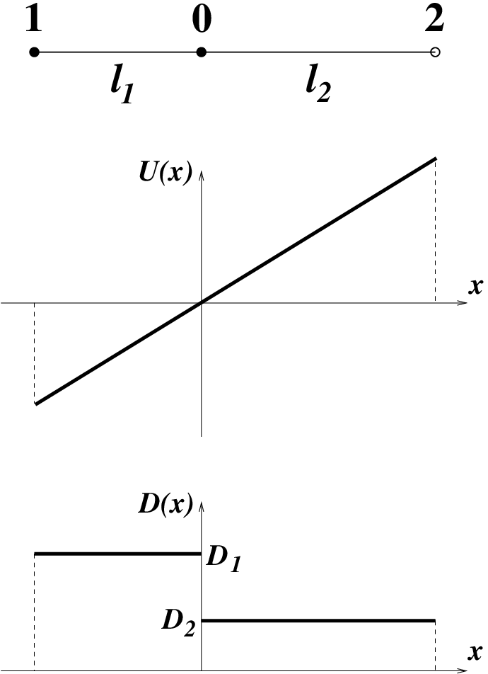
For the graph of Figure 5, the starting point is $0$ , a pure reflection occurs in $1$ ( $p_{10}=1$ ) and the vertex $2$ is absorbing. The potential is $U(x_{02})=a\;x_{02}$ , $U(x_{01})=-a\;x_{01}$ . With the notations of the Figure and using the backward result (39), we get the mean residence time:

	$\displaystyle\mbox{ on the link}\quad[10]\qquad\left\langle\tau_{0}\right\rangle$	$\displaystyle=$	$\displaystyle\frac{p_{01}}{p_{02}}\frac{D_{2}}{a^{2}}\left(e^{al_{2}/D_{2}}-1\right)\left(e^{al_{1}/D_{1}}-1\right)$		(56)
	$\displaystyle\mbox{ on the link}\quad[02]\qquad\left\langle\tau_{0}\right\rangle$	$\displaystyle=$	$\displaystyle\frac{D_{2}}{a^{2}}\left(e^{al_{2}/D_{2}}-1-\frac{al_{2}}{D_{2}}\right)$		(57)

Taking the limit $a\to 0$ (no drift), we obtain:

	$\displaystyle\mbox{ on the link}\quad[10]\qquad\left\langle\tau_{0}\right\rangle$	$\displaystyle=$	$\displaystyle\frac{p_{01}}{p_{02}}\frac{l_{1}l_{2}}{D_{1}}$		(58)
	$\displaystyle\mbox{ on the link}\quad[02]\qquad\left\langle\tau_{0}\right\rangle$	$\displaystyle=$	$\displaystyle\frac{l_{2}^{2}}{2D_{2}}$		(59)

Turning to the forward equation, still with ${\cal P}(y)\equiv\int_{0}^{\infty}{\rm d}t\;P(yt|00)$ , we have

	$\displaystyle\mbox{on the link }[10]\;:\qquad{\cal P}(y_{01})$	$\displaystyle=$	$\displaystyle c_{1}\;e^{ay_{01}/D_{1}}+c_{2}$		(60)
	$\displaystyle\mbox{on the link }[02]\;:\qquad{\cal P}(y_{02})$	$\displaystyle=$	$\displaystyle c_{3}\;e^{-ay_{02}/D_{2}}+c_{4}$		(61)

with the conditions

	$\displaystyle{\cal P}_{(20)}=0\qquad\frac{D_{1}{\cal P}_{(01)}}{p_{01}}=\frac{D_{2}{\cal P}_{(02)}}{p_{02}}\qquad$		$\displaystyle D_{1}{\cal P}^{\prime}_{(10)}+a\;{\cal P}_{(10)}=0$		(62)
	$\displaystyle D_{2}{\cal P}^{\prime}_{(02)}+D_{1}{\cal P}^{\prime}_{(01)}+a\;\left({\cal P}_{(02)}-{\cal P}_{(01)}\right)=-1$				(63)

Computing $\left\langle\tau_{0}\right\rangle=\int_{{\cal D}}{\cal P}(y)\;{\rm d}y$ $\;=c_{1}\frac{D_{1}}{a}\left(e^{al_{1}/D_{1}}-1\right)+c_{2}l_{1}\;$ for the link $[10]$ , $\;=c_{3}\frac{D_{2}}{a}\left(1-e^{-al_{2}/D_{2}}\right)+c_{4}l_{2}\;$ for the link $[02]$ , we recover the solution (56,57).

4.2 Occupation times distribution

Still with the same conditions (drift, spatially-dependent diffusion constant, absorbing vertices,…), we now study a Brownian motion stopped at $t$ and call $T_{\alpha\beta}$ the time spent up to $t$ on the link [ $\alpha\beta$ ].

$T_{\alpha\beta}$ is, of course, a random variable depending on $t$ and we will call ${\cal P}_{t}(\{T_{\alpha\beta}\})$ the joint distribution of the $T_{\alpha\beta}$ ’s.

In the following, we will focus our attention on the quantity

	$\displaystyle S(t\|x0)$	$\displaystyle=$	$\displaystyle\int\prod_{[\alpha\beta]}{\rm d}T_{\alpha\beta}\;{\cal P}_{t}(\{T_{\alpha\beta}\})\;e^{-\sum_{[ij]}\xi_{ij}T_{ij}}$		(64)
		$\displaystyle\equiv$	$\displaystyle\left\langle e^{-\sum_{[ij]}\xi_{ij}T_{ij}}(x)\right\rangle$		(65)

where the $\xi_{ij}$ ’s are positive constants and $\displaystyle\left\langle\ldots(x)\right\rangle$ stands for averaging over all the brownian trajectories starting from $x$ and developing up to $t$ in the presence of the drift.

In order to stick to $S(t|x0)$ , we slightly modify the backward equation (1) by adding, on each link [ $\alpha\beta$ ], a loss term proportional to $\xi_{\alpha\beta}$ ( $\xi_{\alpha\beta}$ may be interpreted as a reaction rate per unit length and time). Thus, we consider the equation:

\frac{\partial Q}{\partial t}=\left(L^{+}(x_{\alpha\beta})-\xi_{\alpha\beta}\right)Q

(66)

where $Q(yt|x0)$ represents the probability of finding the particle in $y$ at time $t$ , each path from $x$ to $y$ being, this time, weighted by a factor $\displaystyle e^{-\sum_{[\alpha\beta]}\xi_{\alpha\beta}T_{\alpha\beta}}$ . (Notice that $Q(yt|x0)=\delta(y-x)$ if $x$ is absorbing).

It is now easy to realize that we have the relationship:

S(t|x0)=\int_{\cal G}{\rm d}y\;Q(yt|x0)

(67)

In the following, we will be especially interested in the Laplace Transform of $S(t|x0)$ :

\widehat{S}(\gamma|x0)\equiv\widehat{S}(x)=\int_{0}^{\infty}{\rm d}t\;e^{-\gamma t}\;S(t|x0)

(68)

On the bond [ $\alpha\beta$ ], $\widehat{S}(x_{\alpha\beta})$ satisfies the following equation ( $\gamma_{\alpha\beta}\equiv\gamma+\xi_{\alpha\beta}$ ):

\left(L^{+}(x_{\alpha\beta})-\gamma_{\alpha\beta}\right)\widehat{S}=-1

(69)

Setting $\displaystyle\widehat{S}(x_{\alpha\beta})=\frac{1}{\gamma_{\alpha\beta}}+\Phi(x_{\alpha\beta})$ and performing the transformation

\Phi(x_{\alpha\beta})=\sqrt{I(x_{\alpha\beta})}\;\chi(x_{\alpha\beta})

(70)

( $I$ is defined in (33)), we are left with the following equation for $\chi$ :

-D\frac{\partial^{2}\chi}{\partial x_{\alpha\beta}^{2}}+\left[\frac{1}{4D}\left(\frac{\partial U(x_{\alpha\beta})}{\partial x_{\alpha\beta}}\right)^{2}-D\frac{\partial}{\partial x_{\alpha\beta}}\left(\frac{1}{2D}\frac{\partial U(x_{\alpha\beta})}{\partial x_{\alpha\beta}}\right)+\gamma_{\alpha\beta}\right]\chi\;=\;0

(71)

Let us call $\chi_{\alpha\beta}$ and $\chi_{\beta\alpha}$ two solutions of (71) such that $\chi_{\alpha\beta}(\alpha)=\chi_{\beta\alpha}(\beta)=1$ , $\chi_{\beta\alpha}(\alpha)=\chi_{\alpha\beta}(\beta)=0$ . So, $\displaystyle\widehat{S}$ writes:

	$\displaystyle\widehat{S}=\frac{1}{\gamma_{\alpha\beta}}$	$\displaystyle+$	$\displaystyle A_{\alpha\beta}\exp\left(\int_{0}^{x_{\alpha\beta}}\frac{{\rm d}z_{\alpha\beta}}{2D(z_{\alpha\beta})}\frac{\partial U(z_{\alpha\beta})}{\partial z_{\alpha\beta}}\right)\chi_{\alpha\beta}(x_{\alpha\beta})$		(72)
		$\displaystyle+$	$\displaystyle A_{\beta\alpha}\exp\left(\int_{l_{\alpha\beta}}^{x_{\alpha\beta}}\frac{{\rm d}z_{\alpha\beta}}{2D(z_{\alpha\beta})}\frac{\partial U(z_{\alpha\beta})}{\partial z_{\alpha\beta}}\right)\chi_{\beta\alpha}(x_{\alpha\beta})$		(72)

The constants $A_{ij}$ are determined by imposing the boundary conditions. Continuity of $\widehat{S}$ at each vertex $\alpha$ implies:

\lim_{{x_{\alpha\beta_{i}}}\to 0}\widehat{S}(x_{\alpha\beta_{i}})\equiv\widehat{S}_{\alpha}=\frac{1}{\gamma_{\alpha\beta_{i}}}+A_{{\alpha\beta_{i}}}

(73)

Moreover, if $\alpha$ is absorbing then $T_{\lambda\mu}=0\ \forall\ [\lambda\mu]$ and, from (64) and (68), we get:

\widehat{S}_{\alpha}=\frac{1}{\gamma}=\frac{1}{\gamma_{\alpha\beta_{i}}}+A_{{\alpha\beta_{i}}}

(74)

Following the same lines as for $\displaystyle\left\langle\tau_{\alpha}\right\rangle$ , it is easy to show that the $\widehat{S}_{\alpha}$ ’s ( $\alpha$ non-absorbing) satisfy a matrix equation with the solution:

\widehat{S}_{\alpha}=\frac{\det R_{1}}{\det R}

(75)

$R$ and $R_{1}$ are again $(V-N)\times(V-N)$ matrices with elements

	$\displaystyle R_{ii}$	$\displaystyle=$	$\displaystyle\sum_{m}p^{\prime}_{{im}}C_{{im}}$		(76)
	$\displaystyle R_{ij}$	$\displaystyle=$	$\displaystyle p^{\prime}_{ij}W_{ij}$		(77)

the quantities $C_{im}$ and $W_{ij}$ being given by:

	$\displaystyle C_{im}$	$\displaystyle=$	$\displaystyle\lim_{{x_{im}}\to 0}\left(\frac{\partial\chi_{im}}{\partial x_{im}}+\frac{\frac{\partial U}{\partial x_{im}}}{2D(x_{im})}\right)$		(78)
	$\displaystyle W_{ij}$	$\displaystyle=$	$\displaystyle\exp\left(\int_{l_{ij}}^{0}\frac{\frac{\partial U}{\partial x_{ij}}}{2D(x_{ij})}{\rm d}x_{ij}\right)\lim_{{x_{ij}}\to 0}\frac{\partial\chi_{ji}}{\partial x_{ij}}$		(79)

$R_{1}=R$ except for the $\alpha^{\mbox{th}}$ column:

\left(R_{1}\right)_{i\alpha}=\sum_{j}\frac{p^{\prime}_{ij}}{\gamma_{ij}}\left(C_{ij}+W_{ij}\right)-\frac{1}{\gamma}\;\sum_{k\;\mbox{abs.}}\;p^{\prime}_{ik}W_{ik}

(80)

(The last summation is performed only over absorbing vertices).

Setting $\xi_{ij}\equiv 0$ , we establish that $\displaystyle\det R_{1}=\frac{1}{\gamma}\det R$ , showing that the probability distribution ${\cal P}_{t}(\{T_{\alpha\beta}\})$ is properly normalized (see (64) and (68)).

Now, let us call $T_{\alpha\beta}^{\prime}$ the time spent on [ $\alpha\beta$ ] before absorption. Thus, for a particle starting from $\alpha$ , we can write

\left\langle e^{-\sum_{[ij]}\xi_{ij}T_{ij}^{\prime}}(\alpha)\right\rangle=\lim_{t\to\infty}\left\langle e^{-\sum_{[ij]}\xi_{ij}T_{ij}}(\alpha)\right\rangle

(81)

and from (65,68) we deduce

\left\langle e^{-\sum_{[ij]}\xi_{ij}T_{ij}^{\prime}}(\alpha)\right\rangle=\lim_{\gamma\to 0}\left(\gamma\widehat{S}_{\alpha}\right)

(82)

Finally, we get:

\left\langle e^{-\sum_{[ij]}\xi_{ij}T_{ij}^{\prime}}(\alpha)\right\rangle=\frac{\det R_{1}^{(0)}}{\det R^{(0)}}

(83)

with $\displaystyle R^{(0)}=\lim_{\gamma\to 0}R$ and $R_{1}^{(0)}=R^{(0)}$ except for the $\alpha^{\mbox{th}}$ column that is given by

\left(R_{1}^{(0)}\right)_{i\alpha}=-\lim_{\gamma\to 0}\;\sum_{k\;\mbox{abs.}}\;p^{\prime}_{ik}W_{ik}

(84)

(84) holds because

\displaystyle\lim_{\gamma\to 0}\left(\frac{\gamma}{\gamma_{ij}}p^{\prime}_{ij}\left(C_{ij}+W_{ij}\right)\right)=0

This is obvious when $\xi_{ij}\neq 0$ . But when $\xi_{ij}=0$ , this is still true because, in that case, $\displaystyle\lim_{\gamma\to 0}\left(C_{ij}+W_{ij}\right)=0$ .

Remark that (84) implies that $\displaystyle\left\langle e^{-\sum_{[ij]}\xi_{ij}T_{ij}^{\prime}}(\alpha)\right\rangle\;=\;0$ if $\cal G$ has no absorbing vertex (in that case, $T^{\prime}_{ij}=\infty$ ).

Setting $\xi_{ij}\equiv\xi$ and $\displaystyle\sum_{[ij]}T^{\prime}_{ij}\equiv\tau$ (survival time), (83) gives the expression of the Laplace Transform of the probability distribution of $\tau$ .

4.2.1 Example

To illustrate this work, let us go back to the example of Figure 2 and study the survival time (parts a) and b) – with $\Delta U=0$ ) and covering time (part c)) distributions.

With a), we get

\left\langle e^{-\xi\tau_{0}}\right\rangle=\;-\;\frac{W_{01}}{C_{01}}

(85)

( $W_{\alpha\beta}$ , $C_{\alpha\beta}$ ,…are computed with $\gamma_{\alpha\beta}=\xi$ ).

b) leads to

\left\langle e^{-\xi\tau_{\lambda}}(q)\right\rangle=\;-\;\frac{q}{Z-1+q}

(86)

with $\displaystyle Z=\frac{C_{01}C_{10}}{W_{01}W_{10}}$

For the covering time $\tau_{c}$ in c) we get (with the notations of (85) and (86)):

	$\displaystyle\left\langle e^{-\xi\tau_{c}}\right\rangle$	$\displaystyle=$	$\displaystyle\;-\;\left\langle e^{-\xi\tau_{0}}\right\rangle\;\prod_{k=1}^{n-1}\left\langle e^{-\xi\tau_{\lambda}}(1-k/n)\right\rangle$		(87)
		$\displaystyle=$	$\displaystyle\;-\;\frac{W_{01}}{C_{01}}\;\frac{(n-1)!}{n^{n-1}}\;\prod_{k=1}^{n-1}\;\frac{1}{Z-\frac{k}{n}}$		(88)

Computation of the first moments shows that when $n\to\infty$ :

	$\displaystyle\left\langle\tau_{c}\right\rangle$	$\displaystyle\propto$	$\displaystyle n\ln n\qquad\mbox{in agreement with }\ (\ref{c3})$		(89)
	$\displaystyle\left\langle\tau_{c}^{2}\right\rangle-\left\langle\tau_{c}\right\rangle^{2}$	$\displaystyle\propto$	$\displaystyle n^{2}$		(90)

Then the probability distribution of the scaling variable $\tau_{c}/\left\langle\tau_{c}\right\rangle$ becomes more and more peaked at its mean value when $n\to\infty$ :

P\left(\frac{\tau_{c}}{\left\langle\tau_{c}\right\rangle}=X\right)\;\to_{n\to\infty}\;\delta(X-1)

(91)

5 First passage times

This section is essentially devoted to a detailed study of exit (or survival) times. First, we will compute exit times distributions and, after, in the last parts, we will focus on quantities concerning exit through a given absorbing vertex.

5.1 Exit times distribution

The density of exit time ${\cal P}(t|x0)$ (without specifying the absorbing vertex) is defined through the loss of probability:

	$\displaystyle{\cal P}(t\|x0)\;{\rm d}t$	$\displaystyle=$	$\displaystyle\int_{{\cal G}}\;{\rm d}y\;P(yt\|x0)-\int_{{\cal G}}\;{\rm d}y\;P(y,t+{\rm d}t\|x0)$		(92)
	$\displaystyle\mbox{Thus:}\quad{\cal P}(t\|x0)$	$\displaystyle=$	$\displaystyle-\frac{\partial}{\partial t}\int_{{\cal G}}\;{\rm d}y\;P(yt\|x0)\;\equiv\;\sum_{\mu\;\mbox{abs.}}{\cal P}_{\mu}(t\|x0)$		(93)

$\displaystyle{\cal P}_{\mu}(t|x0)$ is the density of exit time by the absorbing vertex $\mu$ .

With the forward Fokker-Planck equation, (93) leads to:

$\displaystyle{\cal P}(t\|x0)$	$\displaystyle=$	$\displaystyle-\int_{{\cal G}}\;{\rm d}y\;L(y)P(yt\|x0)=\sum_{\mu\;\mbox{abs.},\;i}J_{\mu\beta_{i}}$	(94)
$\displaystyle J_{\mu\beta_{i}}$	$\displaystyle=$	$\displaystyle\lim_{y_{\mu\beta_{i}}\to 0}\left(\frac{\partial}{\partial y_{\mu\beta_{i}}}(DP)+\frac{\partial U}{\partial y_{\mu\beta_{i}}}P\right)$	(95)
	$\displaystyle=$	$\displaystyle\lim_{y_{\mu\beta_{i}}\to 0}\left(D\frac{\partial P}{\partial y_{\mu\beta_{i}}}\right)$	(96)

because $P_{(\mu\beta_{i})}=0$ when $\mu$ is absorbing. (The $\beta_{i}$ ’s are the nearest-neighbours of $\mu$ on ${\cal G}$ .)

We deduce that $\displaystyle{\cal P}_{\mu}(t|x0)$ is the probability current at vertex $\mu$ : $\displaystyle{\cal P}_{\mu}(t|x0)=\sum_{i}J_{\mu\beta_{i}}$ .

Let us compute the Laplace transform, $\displaystyle\widehat{{\cal P}}(\gamma|x0)$ , of ${\cal P}(t|x0)$ . With (93), we get:

	$\displaystyle\widehat{{\cal P}}(\gamma\|x0)$	$\displaystyle=$	$\displaystyle\int_{0}^{\infty}{\rm d}te^{-\gamma t}\left(-\frac{\partial}{\partial t}\int_{{\cal G}}\;{\rm d}y\;P(yt\|x0)\right)\equiv\sum_{\mu\;\mbox{abs.}}\widehat{{\cal P}}_{\mu}(\gamma\|x0)$		(97)
		$\displaystyle=$	$\displaystyle 1-\gamma\int_{0}^{\infty}{\rm d}te^{-\gamma t}\int_{{\cal G}}\;{\rm d}y\;P(yt\|x0)$		(98)

The backward Fokker-Planck equation gives:

	$\displaystyle L^{+}\widehat{{\cal P}}(\gamma\|x0)$	$\displaystyle=$	$\displaystyle\gamma\widehat{{\cal P}}(\gamma\|x0)$		(99)
	$\displaystyle\mbox{and}\quad L^{+}\widehat{{\cal P}_{\mu}}(\gamma\|x0)$	$\displaystyle=$	$\displaystyle\gamma\widehat{{\cal P}}_{\mu}(\gamma\|x0)$		(100)

Defining $\displaystyle\widehat{{\cal P}}_{\mu,\alpha}=\lim_{x_{\alpha i}\to 0}\widehat{{\cal P}}_{\mu}(\gamma|x_{\alpha i}0)$ , we remark that

\displaystyle\mbox{ for an absorbing vertex }\lambda:\qquad\widehat{{\cal P}}_{\mu,\lambda}\;=\;\delta_{\mu\lambda}

(101)

	$\displaystyle\mbox{This is because}\qquad{\cal P}_{\mu}(t\|\lambda 0)$	$\displaystyle=$	$\displaystyle\delta(t)\qquad\mbox{ if }\quad\lambda=\mu$		(102)
		$\displaystyle=$	$\displaystyle 0\qquad\mbox{ otherwise }$		(103)

Following section 4.2, we readily find, for a particle starting from $\alpha$ (non absorbing), the Laplace transform of the exit (by the vertex $\mu$ ) time distribution:

\widehat{{\cal P}}_{\mu,\alpha}=\frac{\det R_{2}^{(\mu,\alpha)}}{\det R}

(104)

where $R_{2}^{(\mu,\alpha)}=R$ except for the $\alpha^{\mbox{th}}$ column:

\left(R_{2}^{(\mu,\alpha)}\right)_{i\alpha}=\;-p^{\prime}_{i\mu}W_{i\mu}

(105)

$R$ and $W_{i\mu}$ are defined in (76-79) and computed, here, with $\xi_{\alpha\beta}\equiv 0$ . ( $p^{\prime}_{i\mu}$ is defined in (15-16)).

5.2 Splitting probabilities

For a particle starting at $x$ , we define the splitting probability $\Pi_{\mu}(x)$ as the probability of ever reaching the absorbing vertex $\mu$ (rather than any other absorbing vertex). Such a quantity has already been considered for one-dimensional systems [24] (see also [25] for extensions to higher-dimensional systems).

We have, obviously:

\Pi_{\mu}(x)=\int_{0}^{\infty}{\rm d}t\;{\cal P}_{\mu}(t|x0)=\widehat{{\cal P}}_{\mu}(\gamma=0|x0)

(106)

Setting $\gamma=0$ in (100) we see that $\Pi_{\mu}(x)$ satisfies, on $[\alpha\beta]$ , the backward equation:

L^{+}(x_{\alpha\beta})\Pi_{\mu}(x_{\alpha\beta})=0

(107)

The probability, $\Pi_{\mu,\alpha}$ , for a particle starting from the vertex $\alpha$ to be absorbed by $\mu$ , is defined as $\displaystyle\Pi_{\mu,\alpha}=\lim_{x_{\alpha i}\to 0}\Pi_{\mu}(x_{\alpha i})$ .

With (106) and (101), it is easy to realize that

\displaystyle\mbox{ for an absorbing vertex }\lambda:\qquad\Pi_{\mu,\lambda}\;=\;\delta_{\mu\lambda}

(108)

Following the same lines as previously (see section 4.1), we find that $\Pi_{\mu,\alpha}$ ( $\alpha$ non absorbing) is again written as the ratio of two determinants:

\Pi_{\mu,\alpha}=\frac{\det M_{2}^{(\mu,\alpha)}}{\det M}

(109)

where $M_{2}^{(\mu,\alpha)}=M$ except for the $\alpha^{\mbox{th}}$ column:

\left(M_{2}^{(\mu,\alpha)}\right)_{i\alpha}=\;\frac{p^{\prime}_{i\mu}}{J_{(i\mu)}}

(110)

( $M$ is defined in (40,41) and $J_{(i\mu)}$ in (37)).

With simple manipulations on determinants, we check the normalization condition $\displaystyle\sum_{i\;\mbox{abs.}}\Pi_{i,\alpha}=1$ .

Let us, for one moment, comment the case when there is no drift ( $U(x)$ constant but $D(x)$ variable, eventually discontinuous at some vertices). In that case $p^{\prime}_{ij}=p_{ij}$ and, also, $J_{(ij)}=l_{ij}$ . We conclude that the splitting probabilities don’t depend on the varying diffusion constant when there is no drift. This fact can be understood in the following way. Let us consider a discretization of each link and a continuous time. Modifying the diffusion constant amounts to change the waiting time at each site of the discretized graph. But, this would not change the trajectories if there is no drift. Only the time spent is changed. Finally, the splitting probabilities remain unaffected²² 2 For a graph ${\cal G}$ without drift, we could expect, with the same argument, that the average time spent on a part ${\cal D}$ of ${\cal G}$ would not depend on the diffusion constant on the rest, ${\cal G}\backslash{\cal D}$ , of the graph. This is exactly what can be checked with the formulae (39-42) of section 4.1 and, also, with the formulae (58,59) of the example 3 of section 4.1.1. by a change of $D(x)$ .

5.2.1 Example

Let us consider a star-graph without drift. The root $0$ has $m_{0}$ neighbours, all absorbing. The $m_{0}$ links have lengths $l_{0i}$ , $i=1,...,m_{0}$ . With (109), we obtain

\Pi_{i,0}=\left(\frac{p_{0i}}{l_{0i}}\right)\bigg/\left(\sum_{m=1}^{m_{0}}\frac{p_{0m}}{l_{0m}}\right)

(111)

5.3 Conditional mean first passage times

We now turn to the study of the conditional mean first passage time $\left\langle t_{\mu}(x)\right\rangle$ , which is defined as the mean exit time, given that exit is through the absorbing vertex $\mu$ (rather than any other absorbing vertex). We set $\displaystyle\left\langle t_{\mu,\alpha}\right\rangle=\lim_{x_{\alpha i}\to 0}\left\langle t_{\mu}(x_{\alpha i})\right\rangle$ .

Actually, it is simpler to first compute the quantity $\displaystyle\theta_{\mu}(x)\equiv\Pi_{\mu}(x)\left\langle t_{\mu}(x)\right\rangle$ .

Indeed, we have:

$\displaystyle\theta_{\mu}(x)$	$\displaystyle=$	$\displaystyle\int_{0}^{\infty}{\rm d}t\;t\;{\cal P}_{\mu}(t\|x0)$	(112)
$\displaystyle L^{+}\theta_{\mu}(x)$	$\displaystyle=$	$\displaystyle\int_{0}^{\infty}{\rm d}t\;t\;\frac{\partial}{\partial t}{\cal P}_{\mu}(t\|x0)=-\int_{0}^{\infty}{\rm d}t\;{\cal P}_{\mu}(t\|x0)$	(113)
$\displaystyle\mbox{So, we get: }\quad L^{+}\theta_{\mu}(x)$	$\displaystyle=$	$\displaystyle-\;\Pi_{\mu}(x)$	(114)

Moreover, for any absorbing vertex $\lambda$ , we get: $\displaystyle\theta_{\mu,\lambda}=\Pi_{\mu,\lambda}\left\langle t_{\mu,\lambda}\right\rangle=\delta_{\mu,\lambda}\left\langle t_{\mu,\mu}\right\rangle=0$ because $\displaystyle\left\langle t_{\mu,\mu}\right\rangle=0$ .

Thus, comparing this equation with eq.(30), we find for a particle starting from the vertex $\alpha$

\Pi_{\mu,\alpha}\left\langle t_{\mu,\alpha}\right\rangle=\frac{\det M_{3}^{(\mu,\alpha)}}{\det M}

(115)

where $M_{3}^{(\mu,\alpha)}=M$ except for the $\alpha^{\mbox{th}}$ column:

\left(M_{3}^{(\mu,\alpha)}\right)_{i\alpha}\;=\;\sum_{m}p^{\prime}_{im}\frac{\widetilde{K}^{(\mu)}_{(im)}}{J_{(im)}}

(116)

with

\displaystyle\widetilde{K}^{(\mu)}_{(ij)}

\displaystyle=

\displaystyle\int_{0}^{l_{ij}}{\rm d}u_{ij}\;I(u_{ij})\left(\int_{0}^{u_{ij}}{\rm d}z_{ij}\;\frac{\Pi_{\mu}(z_{ij})}{D(z_{ij})I(z_{ij})}\right)\

(117)

In this last equation, $\Pi_{\mu}(z_{ij})$ has to be computed by equation

\Pi_{\mu}(z_{ij})=\Pi_{\mu,i}+\frac{\Pi_{\mu,j}-\Pi_{\mu,i}}{J_{(ij)}}\;\int_{0}^{z_{ij}}{\rm d}u_{ij}\;I(u_{ij})

(118)

with $\Pi_{\mu,i}$ given by eq.(109).

5.3.1 Example

With the same star-graph as in section 5.2.1 (no drift) and a diffusion constant equal to $D_{0i}$ on each link $[0i]$ , we get (111,115)

\left\langle t_{\mu,0}\right\rangle\;=\;\frac{1}{6}\frac{l_{0\mu}^{2}}{D_{0\mu}}\;+\;\frac{1}{3}\left(\sum_{m=1}^{m_{0}}p_{0m}\frac{l_{0m}}{D_{0m}}\right)\bigg/\left(\sum_{m=1}^{m_{0}}\frac{p_{0m}}{l_{0m}}\right)

(119)

6 Summary

We have used the Fokker-Planck Equation (mainly the backward one) to compute some quantities relevant for the study of a Brownian particle moving on a graph. This particle, moving with a varying diffusion constant, is also subjected to a drift.

Being aware that this point is somewhat controversial (see, for instance, [26]), we have discussed in great details the boundary conditions in vertices where either $U(x)$ or $D(x)$ is discontinuous. Two Appendices support the study of those boundary conditions.

Those preliminaries allowed us to deal with various quantities such as the mean residence time, the occupation times probabilities, the splitting probabilities and the conditional mean first passage time. In each case, we have established general formulae that can be used for all kinds of graphs.

Finally, we have checked, on several examples, the consistency of the boundary conditions we have put forward.

Appendix A Backward Equation: boundary conditions when $p_{01}=p_{02}$

For a direct computation of the boundary conditions, it is simpler to consider the Laplace Transform:

\widehat{S}(\gamma|x0)\;=\;\int_{0}^{\infty}{\rm d}t\;e^{-\gamma t}\int_{{\cal G}}{\rm d}yP(yt|x0)

(120)

that satisfies the backward equation ( $\widehat{S}(\gamma|x0)\equiv\widehat{S}(x)$ ):

(L^{+}-\gamma)\widehat{S}(x)\;=\;-1

(121)

First, we want to study the case (A)

For the simple graph of Figure 6 a), $D(x)$ is continuous and $U(x)$ is discontinuous at the vertex $0$ . In particular $U_{(01)}\equiv U_{1}\neq U_{(02)}\equiv U_{2};D(0)\equiv D$ . Moreover, vertices $1$ and $2$ are absorbing and, in $0$ , the transition probabilities are equal: $p_{01}=p_{02}=1/2$ .

Now, let us add to this graph, the link $[03]$ of length $L$ (see Figure 6 b)) in such a way that nothing is changed for the rest (for example, the potential on the link $[02]$ of the original graph is the same as the one on the link $[32]$ of the modified graph, …). On $[03]$ , we define $U(x_{03})=\left(\frac{U_{2}-U_{1}}{L}\right)x_{03}+U_{1}$ and $D(x_{03})\equiv D$ . When $L\to 0$ , we recover Figure 6 a).

Working with this modified graph, the solution of (121) writes:

$\displaystyle\mbox{on the link }\;[10]\qquad\widehat{S}(x_{10})$	$\displaystyle=$	$\displaystyle 1/\gamma+a_{1}\phi_{1}(x_{10})+a_{2}\phi_{2}(x_{10})$	(122)
$\displaystyle\mbox{on the link }\;[03]\qquad\widehat{S}(x_{03})$	$\displaystyle=$	$\displaystyle 1/\gamma+c_{1}e^{r_{+}x_{03}}+c_{2}e^{r_{-}x_{03}}$	(123)
$\displaystyle\mbox{on the link }\;[32]\qquad\widehat{S}(x_{32})$	$\displaystyle=$	$\displaystyle 1/\gamma+b_{1}\psi_{1}(x_{32})+b_{2}\psi_{2}(x_{32})$	(124)

with

	$\displaystyle r_{\pm}$	$\displaystyle=$	$\displaystyle\frac{A\pm\sqrt{A^{2}+4\gamma D}}{2D}$		(125)
	$\displaystyle A$	$\displaystyle=$	$\displaystyle\frac{U_{2}-U_{1}}{L}$		(126)

$\phi_{1,2}$ and $\psi_{1,2}$ are solutions of the equation $(L^{+}-\gamma)\phi=0$ that satisfy ( $\phi_{(\alpha\beta)}\equiv\lim_{x_{\alpha\beta}\to 0}\phi(x_{\alpha\beta})$ ):

	$\displaystyle\phi_{1\;(10)}=0\quad\phi_{1\;(01)}=1$		$\displaystyle\phi_{2\;(10)}=1\quad\phi_{2\;(01)}=0$		(127)
	$\displaystyle\psi_{1\;(32)}=1\quad\psi_{1\;(23)}=0$		$\displaystyle\psi_{2\;(32)}=0\quad\psi_{2\;(23)}=1$		(128)

$U(x)$ and $D(x)$ are continuous everywhere on the graph. So, we write standard boundary conditions at the vertices (continuity of $\widehat{S}$ and its derivative at vertices $0$ and $3$ ; $\widehat{S}=0$ at vertices $1$ and $2$ ). We obtain ( $\phi^{\prime}_{(\alpha\beta)}\equiv\lim_{x_{\alpha\beta}\to 0}\frac{\partial\phi(x_{\alpha\beta})}{\partial x_{\alpha\beta}}$ ):

$\displaystyle a_{2}=b_{2}=-\frac{1}{\gamma}\qquad a_{1}=c_{1}+c_{2}$		$\displaystyle b_{1}=c_{1}e^{r_{+}L}+c_{2}e^{r_{-}L}$	(129)
$\displaystyle a_{1}\phi^{\prime}_{1\;(01)}+a_{2}\phi^{\prime}_{2\;(01)}+c_{1}r_{+}+c_{2}r_{-}$	$\displaystyle=$	$\displaystyle 0$	(130)
$\displaystyle b_{1}\psi^{\prime}_{1\;(32)}+b_{2}\psi^{\prime}_{2\;(32)}-c_{1}r_{+}e^{r_{+}L}-c_{2}r_{-}e^{r_{-}L}$	$\displaystyle=$	$\displaystyle 0$	(131)

After some algebra, we get the results:

	$\displaystyle\frac{\widehat{S}_{(32)}}{\widehat{S}_{(01)}}$	$\displaystyle=$	$\displaystyle\frac{\frac{1}{\gamma}+b_{1}}{\frac{1}{\gamma}+a_{1}}\to_{L\to 0}\;1$		(132)
	$\displaystyle\frac{\widehat{S}^{\prime}_{(32)}}{\widehat{S}^{\prime}_{(01)}}$	$\displaystyle=$	$\displaystyle\frac{b_{1}\psi^{\prime}_{1\;(32)}+b_{2}\psi^{\prime}_{2\;(32)}}{a_{1}\phi^{\prime}_{1\;(01)}+a_{2}\phi^{\prime}_{2\;(01)}}\to_{L\to 0}\;-\;e^{(U_{2}-U_{1})/D}$		(133)

When $L\to 0$ , the vertex $3$ moves to $0$ and equations (132) and (133) give, for the original graph:

	$\displaystyle\widehat{S}_{(01)}$	$\displaystyle=$	$\displaystyle\widehat{S}_{(02)}$		(134)
	$\displaystyle\widehat{S}^{\prime}_{(01)}e^{-U_{(01)}/D(0)}$	$\displaystyle+$	$\displaystyle\widehat{S}^{\prime}_{(02)}e^{-U_{(02)}/D(0)}=0$		(135)

In particular, we observe that $\widehat{S}$ is continuous at $0$ and that exponential factors appear in the condition involving the derivatives.

Let us now turn to the case (B), still with the same graph and $p_{01}=p_{02}=1/2$ .

This time (Figure 7 a)), $D(x)$ is discontinuous at $0$ and $U(x)$ is continuous. We set: $D_{(01)}\equiv D_{1}\neq D_{(02)}\equiv D_{2}$ , $U(0)\equiv U$ .

As we already did for the case (A), we modify the graph and obtain Figure 7 b). Between vertices $0$ and $3$ , we choose: $U(x_{03})=U$ and $\displaystyle D(x_{03})=\left(\left(\frac{\sqrt{D_{2}}-\sqrt{D_{1}}}{L}\right)x_{03}+\sqrt{D_{1}}\right)^{2}\;\equiv\;(ax_{03}+b)^{2}$ . Thus, in the modified graph, $D(x)$ and $U(x)$ are continuous everywhere on the graph.

On the links $[10]$ and $[32]$ , the solution of equation (121) is still given by (122) and (124) (with the conditions (127) and (128)). But, on the link $[03]$ , (123) has to be replaced by

$\displaystyle\qquad\widehat{S}(x_{03})$	$\displaystyle=$	$\displaystyle 1/\gamma+c_{1}\;(a\;x_{03}+b)^{\lambda_{+}}+c_{2}\;(a\;x_{03}+b)^{\lambda_{-}}$	(136)
$\displaystyle\mbox{with:}\qquad\lambda_{\pm}$	$\displaystyle=$	$\displaystyle\frac{1}{2}\pm\frac{1}{2}\sqrt{1+\frac{4\gamma}{a^{2}}}$	(137)
$\displaystyle a$	$\displaystyle=$	$\displaystyle\frac{\sqrt{D_{2}}-\sqrt{D_{1}}}{L}$	(138)

Standard boundary conditions imply:

$\displaystyle a_{2}=b_{2}=-\frac{1}{\gamma}\qquad a_{1}=c_{1}D_{1}^{\lambda_{+}/2}+c_{2}D_{1}^{\lambda_{-}/2}\qquad b_{1}=c_{1}D_{2}^{\lambda_{+}/2}+c_{2}D_{2}^{\lambda_{-}/2}$			(139)
$\displaystyle a_{1}\phi^{\prime}_{1\;(01)}+a_{2}\phi^{\prime}_{2\;(01)}+a\left(c_{1}\lambda_{+}D_{1}^{(\lambda_{+}-1)/2}+c_{2}\lambda_{-}D_{1}^{(\lambda_{-}-1)/2}\right)$	$\displaystyle=$	$\displaystyle 0$	(140)
$\displaystyle b_{1}\psi^{\prime}_{1\;(32)}+b_{2}\psi^{\prime}_{2\;(32)}-a\left(c_{1}\lambda_{+}D_{2}^{(\lambda_{+}-1)/2}+c_{2}\lambda_{-}D_{2}^{(\lambda_{-}-1)/2}\right)$	$\displaystyle=$	$\displaystyle 0$	(141)

Finally, we get:

	$\displaystyle\frac{\widehat{S}_{(32)}}{\widehat{S}_{(01)}}$	$\displaystyle=$	$\displaystyle\frac{\frac{1}{\gamma}+b_{1}}{\frac{1}{\gamma}+a_{1}}\to_{L\to 0}\;\;1$		(142)
	$\displaystyle\frac{\widehat{S}^{\prime}_{(32)}}{\widehat{S}^{\prime}_{(01)}}$	$\displaystyle=$	$\displaystyle\frac{b_{1}\psi^{\prime}_{1\;(32)}+b_{2}\psi^{\prime}_{2\;(32)}}{a_{1}\phi^{\prime}_{1\;(01)}+a_{2}\phi^{\prime}_{2\;(01)}}\to_{L\to 0}\;\;-\;1$		(143)

When $L\to 0$ , we get, for the original graph, $\widehat{S}$ continuous in $0$ and

\widehat{S}^{\prime}_{(01)}\;+\;\widehat{S}^{\prime}_{(02)}\;=\;0

(144)

Appendix B Backward Equation: boundary conditions when $p_{01}\neq p_{02}$

We want to study the case (A) ( $U(x)$ discontinuous in $0$ ) for the graph of Figure 8 a) with, this time, $p_{01}\neq p_{02}$ .

Modifying this graph, we obtain a new one, consisting in five vertices, displayed in Figure 8 b). Vertices $1$ and $2$ are still absorbing. We set $p_{41}=p_{40}=p_{30}=p_{32}=1/2$ but $p_{04}\neq p_{03}$ ( $p_{04}=p_{01}$ (original graph) and $p_{03}=p_{02}$ (original graph)).

$U(x)$ (resp. $D(x)$ ) is set equal to some constant $U$ (resp. $D$ ) on the added links $[40]$ and $[03]$ . $U(x)$ is discontinuous at vertices $4$ and $3$ . With the modified graph, we can take advantage of the computations of the boundary conditions performed at the beginning of section 3 and also in Appendix A.

The solution of equation (121) writes:

$\displaystyle\mbox{on the link }\;[14]\qquad\widehat{S}(x_{14})$	$\displaystyle=$	$\displaystyle 1/\gamma+a_{1}\phi_{1}(x_{14})+a_{2}\phi_{2}(x_{14})$	(145)
$\displaystyle\mbox{on the link }\;[40]\qquad\widehat{S}(x_{40})$	$\displaystyle=$	$\displaystyle 1/\gamma+b_{1}\sinh(\sqrt{\gamma/D}x_{40})+b_{2}\sinh(\sqrt{\gamma/D}(L-x_{40}))$	(146)
$\displaystyle\mbox{on the link }\;[03]\qquad\widehat{S}(x_{03})$	$\displaystyle=$	$\displaystyle 1/\gamma+c_{1}\sinh(\sqrt{\gamma/D}x_{03})+c_{2}\sinh(\sqrt{\gamma/D}(L^{\prime}-x_{03}))$	(147)
$\displaystyle\mbox{on the link }\;[32]\qquad\widehat{S}(x_{32})$	$\displaystyle=$	$\displaystyle 1/\gamma+d_{1}\psi_{1}(x_{32})+d_{2}\psi_{2}(x_{32})$	(148)

As before, $\phi_{1,2}$ and $\psi_{1,2}$ are solutions of the equation $(L^{+}-\gamma)\phi=0$ that satisfy:

	$\displaystyle\phi_{1\;(14)}=0\quad\phi_{1\;(41)}=1$		$\displaystyle\phi_{2\;(14)}=1\quad\phi_{2\;(41)}=0$		(149)
	$\displaystyle\psi_{1\;(32)}=1\quad\psi_{1\;(23)}=0$		$\displaystyle\psi_{2\;(32)}=0\quad\psi_{2\;(23)}=1$		(150)

The boundary conditions in $0$ are given by the beginning of section 3.1. $\widehat{S}$ is continuous and

p_{04}\;\widehat{S}^{\prime}_{(04)}\;+\;p_{03}\;\widehat{S}^{\prime}_{(03)}\;=\;0

(151)

For vertices $4$ and $3$ , we use the result of Appendix A (case (A)). $\widehat{S}$ is again continuous and

	$\displaystyle\widehat{S}^{\prime}_{(41)}e^{-U_{1}/D}\;+\;\widehat{S}^{\prime}_{(40)}e^{-U/D}$	$\displaystyle=$	$\displaystyle 0$		(152)
	$\displaystyle\widehat{S}^{\prime}_{(30)}e^{-U/D}\;+\;\widehat{S}^{\prime}_{(32)}e^{-U_{2}/D}$	$\displaystyle=$	$\displaystyle 0$		(153)

We get the relationships:

$\displaystyle a_{2}=d_{2}=-\frac{1}{\gamma}\qquad a_{1}=b_{2}\sinh(\sqrt{\gamma/D}L)\qquad d_{1}=c_{1}\sinh(\sqrt{\gamma/D}L^{\prime})$			(154)
$\displaystyle b_{1}\sinh(\sqrt{\gamma/D}L)=c_{2}\sinh(\sqrt{\gamma/D}L^{\prime})$			(155)
$\displaystyle p_{04}\left(-b_{1}\cosh(\sqrt{\gamma/D}L)+b_{2}\right)\;+\;p_{03}\left(c_{1}-c_{2}\cosh(\sqrt{\gamma/D}L^{\prime})\right)$	$\displaystyle=$	$\displaystyle 0$	(156)
$\displaystyle\left(a_{1}\phi^{\prime}_{1\;(41)}+a_{2}\phi^{\prime}_{2\;(41)}\right)e^{-U_{1}/D}\;+\;\sqrt{\gamma/D}\left(b_{1}-b_{2}\cosh(\sqrt{\gamma/D}L)\right)e^{-U/D}$	$\displaystyle=$	$\displaystyle 0$	(157)
$\displaystyle\left(d_{1}\psi^{\prime}_{1\;(32)}+d_{2}\psi^{\prime}_{2\;(32)}\right)e^{-U_{2}/D}\;-\;\sqrt{\gamma/D}\left(c_{1}\cosh(\sqrt{\gamma/D}L^{\prime})-c_{2}\right)e^{-U/D}$	$\displaystyle=$	$\displaystyle 0$	(158)

Solving and taking the limit $L,L^{\prime}\to 0$ , we are left with:

	$\displaystyle\frac{\widehat{S}_{(32)}}{\widehat{S}_{(41)}}=\frac{\frac{1}{\gamma}+d_{1}}{\frac{1}{\gamma}+a_{1}}\to_{L,L^{\prime}\to 0}$		$\displaystyle 1$		(159)
	$\displaystyle\frac{\widehat{S}^{\prime}_{(32)}}{\widehat{S}^{\prime}_{(41)}}=\frac{d_{1}\psi^{\prime}_{1\;(32)}+d_{2}\psi^{\prime}_{2\;(32)}}{a_{1}\phi^{\prime}_{1\;(41)}+a_{2}\phi^{\prime}_{2\;(41)}}\to_{L,L^{\prime}\to 0}$		$\displaystyle e^{\frac{U_{2}-U_{1}}{D}}\left(\;-\;\frac{p_{04}}{p_{03}\;}\right)$		(160)

When $L,L^{\prime}\to 0$ , the vertices $3$ and $4$ move to $0$ and we get³³ 3 Recall that $p_{04}=p_{01}$ (original graph) and $p_{03}=p_{02}$ (original graph).:

	$\displaystyle\widehat{S}_{(02)}$	$\displaystyle=$	$\displaystyle\widehat{S}_{(01)}$		(161)
	$\displaystyle p_{02}\;\widehat{S}^{\prime}_{(02)}\;e^{-U_{(02)}/D(0)}\;+\;p_{01}\;\widehat{S}^{\prime}_{(01)}\;e^{-U_{(01)}/D(0)}$	$\displaystyle=$	$\displaystyle 0$		(162)

We also observe that:

	$\displaystyle\frac{\widehat{S}_{(03)}}{\widehat{S}_{(30)}}\to_{L,L^{\prime}\to 0}$		$\displaystyle 1$		(163)
	$\displaystyle\frac{\widehat{S}^{\prime}_{(03)}}{\widehat{S}^{\prime}_{(30)}}\to_{L,L^{\prime}\to 0}$		$\displaystyle-\;1$		(164)

Those relationships will show useful in Appendix C.

The solution for the case (B) (Figure 9 a), $p_{01}\neq p_{02}$ ) is immediate.

Indeed, we see that for the modified graph (Figure 9 b)), we have, formally, the same solution as equations (145)-(148) and the same boundary conditions but, this time, with $U_{1}=U_{2}=U$ . It amounts to drop the exponential factors in (152) and in all the equations that follow. Finally, we get that $\widehat{S}$ is continuous and

p_{02}\;\widehat{S}^{\prime}_{(02)}\;+\;p_{01}\;\widehat{S}^{\prime}_{(01)}=0

(165)

Moreover, (163) and (164) still hold.

Appendix C Backward Equation: general boundary conditions

For the case (A), let us assume that the $p_{\alpha\beta_{i}}$ ’s are not all equal. In Figure 10 a), where a given vertex $\alpha$ and its $m_{\alpha}$ nearest-neighbours are shown, we suppose that $U(x)$ is discontinuous in $\alpha$ ( $D(x)$ is continuous, $D(x)\equiv D(\alpha)$ in $\alpha$ ) .

In part b), we slightly modify the graph along the same lines as in Appendix B. We add vertices $\mu_{i}$ in such a way that each new link $[\mu_{i}\beta_{i}]$ is identical to the original link $[\alpha\beta_{i}]$ (same length, same potential and diffusion constant). Moreover, in the added subgraph (Figure 10 b), heavy lines of lengths $L$ ) the potential and the diffusion constant are assumed to be constant (respectively equal to some value $U$ and to $D(\alpha)$ ). So, in the vicinity of $\alpha$ , the discontinuities of $U(x)$ will occur at the $\mu_{i}$ ’s ( $D(x)$ will be continuous in the same domain). Of course, for the transition probabilities from $\alpha$ , we choose $p_{\alpha\mu_{i}}=p_{\alpha\beta_{i}}$ . By taking the limit $L\to 0$ , we will recover the original graph.

Now, for the small subgraph where $U(x)$ and $D(x)$ are constant, we can take advantage of the result, equation (8), to write:

\sum_{i=1}^{m_{\alpha}}\;p_{\alpha\mu_{i}}\;P^{\prime}_{(\alpha\mu_{i})}\;=\;0

(166)

Moreover, for the vertex $\mu_{i}$ , where $p_{\mu_{i}\alpha}=p_{\mu_{i}\beta_{i}}=1/2$ , we can use (11) and also (135) (directly established in Appendix A) to get:

e^{-U/D(\alpha)}P^{\prime}_{(\mu_{i}\alpha)}\;+\;e^{-U_{(\mu_{i}\beta_{i})}/D(\alpha)}P^{\prime}_{(\mu_{i}\beta_{i})}\;=\;0

(167)

Weighting with $p_{\alpha\beta_{i}}(\equiv p_{\alpha\mu_{i}})$ and summing over $i$ , we deduce:

\sum_{i=1}^{m_{\alpha}}\;p_{\alpha\beta_{i}}e^{-U_{(\mu_{i}\beta_{i})}/D(\alpha)}P^{\prime}_{(\mu_{i}\beta_{i})}\;=\;-\;e^{-U/D(\alpha)}\left(\sum_{i=1}^{m_{\alpha}}p_{\alpha\mu_{i}}\;P^{\prime}_{(\mu_{i}\alpha)}\right)

(168)

Now, taking the limit $L\to 0$ , we have from (164) (Appendix B):

\frac{P^{\prime}_{(\mu_{i}\alpha)}}{P^{\prime}_{(\alpha\mu_{i})}}\to_{L\to 0}\;-\;1

(169)

In this limit, the vertex $\mu_{i}$ moves to $\alpha$ and we recover the original graph. Finally, with (166,168,169), we obtain, for the case (A), the boundary condition⁴⁴ 4 Remark that (170) is unchanged when we add a constant to $U(x)$ . Now, if we want to consider the case when $U(x)$ and $D(x)$ are both discontinuous at some vertex $\alpha$ , we must add, on each link, vertices $\mu_{i}$ and $\mu^{\prime}_{i}$ where either $D(x)$ or $U(x)$ are discontinuous. The resulting boundary condition will depend on the repartition of those additional vertices. Moreover, inconsistencies will appear when we add a constant to $U(x)$ . This is why we say that, in our opinion, this problem is ill-defined.:

\sum_{i=1}^{m_{\alpha}}\;p_{\alpha\beta_{i}}\;e^{-U_{(\alpha\beta_{i})}/D(\alpha)}\;P^{\prime}_{(\alpha\beta_{i})}\;=\;0

(170)

Moreover, for the modified graph, $P$ is continuous in $\alpha$ and in $\mu_{i}$ . From Appendix B, we know that (163):

\frac{P_{(\mu_{i}\alpha)}}{P_{(\alpha\mu_{i})}}\to_{L\to 0}\;1

(171)

That’s enough to conclude that, for the original graph, $P$ is continuous in $\alpha$ .

References

[1] Baxter R J 1982 Exactly Solved Models in Statistical Mechanics (London: Academic Press)
[2] Economou E N 1983 Green’s Functions in Quantum Physics (Berlin: Springer)
[3] Cvetkovic D M, Doob M, and Sachs H 1980 Spectra of Graphs, Theory and Application (Academic, New York)
[4] Rudenberg K and Scherr C 1953 J. Chem. Phys. 21 1565
[5] Rammal R 1984 J. Phys. I (France) 45 191
[6] Avron J E and Sadun L 1991 Ann. Phys. (N.Y.) 206 440
[7] C. Texier and G. Montambaux 2001 J. Phys. A Math.Gen. 34 10307
[8] Pascaud M and Montambaux G 1999 Phys. Rev. Lett. 82 4512
[9] Akkermans E, Comtet A, Desbois J, Montambaux G and Texier C 2000 Annals of Physics 284 10
[10] Desbois J 2000 J. Phys. A: Math. Gen. 33 L63
[11] Roth J P 1983 C. R. Acad. Sc. Paris 296 793
[12] Desbois J 2001 Eur. Phys. J. B 24 261
[13] Ihara Y 1966 J. Math. Soc. Japan 18 219 Stark H M and Terras A A 1996 Adv. in Math. 121 124 Wu F Y and Kunz H 1999 Ann. Combin. 3 475
[14] Levy P 1948 Processus Stochastiques et Mouvement Brownien (Paris: Editions Jacques Gabay)
[15] Levy P 1939 Compositio Math. 7 283
[16] Barlow M, Pitman J and Yor M 1989 Sém. Probabilités XXIII (Lecture Notes in Maths vol 1372) (Berlin: Springer) p 294
[17] Desbois J 2002 J. Phys. A: Math. Gen. 35 L673
[18] Comtet A, Desbois J and Majumdar S N 2002 J. Phys. A: Math. Gen. 35 L687
[19] van Kampen N G 1981 Stochastic processes in Physics and Chemistry (Amsterdam: Elsevier)
[20] Redner S 2001 A Guide to First-Passage Processes (Cambridge: Cambridge University Press) Bénichou O, Coppey M, Klafter J, Moreau M and Oshanin G 2005 J. Phys. A: Math. Gen. 38 7205 Bénichou O, Coppey M, Moreau M and Oshanin G 2005 J. Chem. Phys. 123 194506 Condamin S, Bénichou O and Moreau M 2005 Phys. Rev. Lett. 95 260601 Condamin S, Bénichou O and Moreau M 2007 Phys. Rev. E 75 021111
[21] Agmon N 1984 J. Chem. Phys. 81 3644
[22] Risken H 1996 The Fokker-Planck Equation (Berlin: Springer)
[23] Aldous D and Fill J 1999 Reversible Markov chains and random walks on graphs (http://www.stat.berkeley.edu/users/aldous/RWG/book.html)
[24] Gardiner CW 2004 Handbook of Stochastic Methods for Physics, Chemistry and Natural Sciences (Berlin: Springer).
[25] Condamin S, Tejedor V, Voituriez R, Bénichou O and Klafter J 2008 Proc. Natl. Acad. Sci. USA 105 5675
[26] Kim I C and Torquato S 1990 J. Appl. Phys. 68 3892 Torquato S, Kim I C and Cule D 1999 J. Appl. Phys. 85 1560

Exit and Occupation times for Brownian Motion on Graphs with General Drift and Diffusion Constant

Abstract

1 Introduction

2 Definitions and notations

3 Boundary conditions

3.1 Backward Fokker-Planck equation

3.2 Forward Fokker-Planck equation

4 Occupation times

4.1 Mean residence time

4.1.1 Examples

4.2 Occupation times distribution

4.2.1 Example

5 First passage times

5.1 Exit times distribution

5.2 Splitting probabilities

5.2.1 Example

5.3 Conditional mean first passage times

5.3.1 Example

6 Summary

Appendix A Backward Equation: boundary conditions when p01=p02p_{01}=p_{02}

Appendix B Backward Equation: boundary conditions when p01≠p02p_{01}\neq p_{02}

Appendix C Backward Equation: general boundary conditions

References

Appendix A Backward Equation: boundary conditions when $p_{01}=p_{02}$

Appendix B Backward Equation: boundary conditions when $p_{01}\neq p_{02}$