跳到论文正文
W Papers独立论文阅读器 arXiv:0810.4545 论文正文 计算阅读时间 · 0%
引用这篇论文根据当前论文元数据生成,正式投稿前建议核对。


License: arXiv.org perpetual non-exclusive license
arXiv:0810.4545v3 [hep-ph] 12 Feb 2009

t​b​WtbW vertex in the
Littlest Higgs Model with T-parity

F. Peñuñuri 1,  F. Larios 2 Affiliation: 1 Facultad de Ingenieria, Universidad Autónoma de Yucatán, A.P. 150, Cordemex, Mérida, Yucatan, México.
2Departamento de Física Aplicada, CINVESTAV-Mérida, A.P. 73, 97310 Mérida, Yucatán, México
Abstract

A study of the effective t​b​WtbW vertex is done in the littlest Higgs model with T parity that includes the one loop induced weak dipole coefficient f2​Rf_{2R}. The top’s width, the W-boson helicity in the t→b​W+t\to bW^{+} decay as well as the t-channel and the s-channel modes of single top quark production at the LHC are then obtained for the t​b​WtbW coupling. Our calculation is done in the Feynman-’t Hooft gauge, and we provide details of the analysis, like exact formulas (to all orders of the expansion variable v/fv/f) of masses and mixing angles of all the particles involved. Also, a complete and exact diagonalization (and normalization) of the scalar sector of the model is made.

pacs
 12.60.Cn, 12.60.Fr

I Introduction

The Top quark plays a major role in the research program of the LHC. The top is the only quark that decays Weakly before hadronization, therefore we have an opportunity to study bare quark properties like spin, mass and couplings[1, 2]. Recent measurements of the single top quark production as well as the W-helicity in the t→b​W+t\to bW^{+} decay have been made by the D0 and CDF groups at the Tevatron and these have (for the first time) set direct constraints on the effective t​b​WtbW vertex[3]. On the other hand, the high production of top quarks at the LHC will make it possible to probe directly this vertex down to a few percent deviation level for the left handed coefficient f1​Lf_{1L}, and to set limits of order 10−210^{-2} for f2​Rf_{2R}, and of order 10−110^{-1} for the right handed f1​Rf_{1R} and f1​Lf_{1L}[4]. From the theoretical standpoint, observables that depend directly on the t​b​WtbW coupling like single top production, the top’s width and the W-helicity in top’s decay have been studied in models beyond the SM like the minimal supersymmetric standard model [5] and the Topcolor assisted Technicolor (TC2) model[6].

In the Standard Model (SM) the Higgs boson receives large quadratic divergent corrections from the heavy gauge bosons and from this fermion. Models beyond the SM are studied that alleviate this problem, two important examples are Supersymmetry and Technicolor (and TC2)[7]. Another possible solution is provided by the recently proposed Little Higgs Models[8, 9] (for a review see Ref. [10]). In these models the quadratic divergent Higgs mass corrections get canceled at the one loop level via the contribution from certain (very heavy) partners of the gauge bosons and the top quark (i.e. the WH±W_{H}^{\pm} boson, the ZHZ_{H} boson and the TT quark). One explicit model has become well known, and it is called the “Littlest Higgs Model” (LH)[9]. The LH model is based on a non-linear sigma model of an S​U​(5)/S​O​(5)SU(5)/SO(5) global symmetry breaking. It consists of two S​U​(2)×U⁡(1)SU(2)\times U(1) gauge symmetries that break down to the SM gauge symmetry at a certain scale ff. The phenomenology of the model deals with heavy partners of the SM gauge bosons, like WH±W_{H}^{\pm}, ZHZ_{H} and a heavy photon AHA_{H}, as well as a heavy partner of the top quark TT[11]. These heavy partners mix with the lighter SM gauge bosons and this gives rise to tree level contributions to precision electroweak observables. Therefore, strong constraints have greatly limited the parameter range of the model (for instance: f≥4f\geq 4 TeV)[12]. A way out of this obstacle is given by implementing a new symmetry called T-parity, where T-parity even and T-parity odd particles do not mix[13]. There is one model that is often studied in the literature; it is based on the previous LH model and is known as the Littlest Higgs Model with T-parity (LHT)[14]. Electroweak precision constraints for the LHT model allow the scale ff to be as low as ∼500\sim 500 GeV[15]. This model has therefore received more attention recently, with many phenomenological studies on production and decays of the new heavy particles[16] as well as theoretical studies such as T-parity violation[17], top quark induced vacuum alignment[18], and two vacuum expectation value (VEV) scales ff in LH models[19].

In this paper we study the t​b​WtbW vertex in the context of the Littlest Higgs Model with T-parity (LHT). We will often refer to and will use the notation of Ref. [20]. A detailed explanation of the model can be found in Refs. [20, 21]. In this work we focus on the interactions that are relevant to the study of the effective t​b​WtbW vertex.

In the literature an expansion in powers of ϵ=v/f\epsilon=v/f is usually made for the masses and mixing angles derived from the Lagrangian of the model. Here, we have obtained the exact (all powers in ϵ≡v/f\epsilon\;\equiv v/f) formulas for masses and mixings. Similar expressions have already appeared in Ref. [22] and we have found agreement. Moreover, we provide in detail the diagonalization procedure of the scalar sector, including the Goldstone bosons that are eaten by the gauge bosons and that participate in the one-loop calculation as is done in the Feynman-t’Hooft gauge. We provide Feynman rules that are not found in previous studies of the model.

The next section has the brief presentation of the LHT Lagrangians (Kinetic and Yukawa) and the definition of mass eigenstate fields in terms of the original interaction eigenstates. Then, in the following section, we will discuss the effective t​b​WtbW vertex obtained from tree and one-loop level contributions. From this effective vertex we compute some of the observables associated to the top quark, like the top’s decay width, the W-boson helicity in the t→b​W+t\to bW^{+} decay, the single top production process in the two most important modes: the t-channel and the s-channel.

II The Littlest Higgs Model with T-parity.

The LHT model is based on a non-linear sigma model for an S​U​(5)/S​O​(5)SU(5)/SO(5) symmetry breaking. The non-linear Σ\Sigma field is given as[15]

Σ=e2​i​Π/f​Σ0,withΣ0=(𝟎2×2𝟎2×1𝟏2×2𝟎1×21𝟎1×2𝟏2×2𝟎2×1𝟎2×2).\displaystyle\Sigma=e^{2i\Pi/f}\Sigma_{0}\;\;,\;\;{\rm with}\;\;\;\;\Sigma_{0}=\left(\begin{array}[]{ccc}{\bf 0}_{2\times 2}&{\bf 0}_{2\times 1}&{\bf 1}_{2\times 2}\\ {\bf 0}_{1\times 2}&1&{\bf 0}_{1\times 2}\\ {\bf 1}_{2\times 2}&{\bf 0}_{2\times 1}&{\bf 0}_{2\times 2}\\ \end{array}\right).

where f∼𝒪⁡(1)f\sim{\cal O}(1) TeV is the symmetry breaking scale known as the “pion decay constant”. The “pion matrix” contains a total of 14 pion fields[15]:

Π=(−ω0/2−η/20−ω+/2−iπ+/2−i​ϕ+⁣+−iϕ+/2−ω−/2ω0/2−η/20(v+h+i​π0)/2−iϕ+/2(−i​ϕ0+ϕP0)/2i​π−/2(v+h−i​π0)/24/5​η−iπ+/2(v+h+i​π0)/2i​ϕ−⁣−i​ϕ−/2i​π−/2−ω0/2−η/20−ω−/2i​ϕ−/2(i​ϕ0+ϕP0)/2(v+h−i​π0)/2−ω+/2ω0/2−η/20),\displaystyle\Pi\,=\left(\!\!\begin{array}[]{ccccc}-\omega^{0}/2-\eta/\sqrt{20}&-\omega^{+}/\sqrt{2}&-i\pi^{+}/\sqrt{2}&-i\phi^{++}&-i{\phi^{+}}/{\sqrt{2}}\\ -\omega^{-}/\sqrt{2}&\omega^{0}/2-\eta/\sqrt{20}&(v+h+i\pi^{0})/2&-i{\phi^{+}}/{\sqrt{2}}&(-i\phi^{0}+\phi_{P}^{0})/{\sqrt{2}}\\ i\pi^{-}/\sqrt{2}&(v+h-i\pi^{0})/2&\sqrt{4/5}\eta&-i\pi^{+}/\sqrt{2}&(v+h+i\pi^{0})/2\\ i\phi^{--}&i{\phi^{-}}/{\sqrt{2}}&i\pi^{-}/\sqrt{2}&-\omega^{0}/2-\eta/\sqrt{20}&-\omega^{-}/\sqrt{2}\\ i{\phi^{-}}/{\sqrt{2}}&(i\phi^{0}+\phi_{P}^{0})/{\sqrt{2}}&(v+h-i\pi^{0})/{2}&-\omega^{+}/\sqrt{2}&\omega^{0}/2-\eta/\sqrt{20}\end{array}\!\!\right),

Seven of these fields get eaten by the gauge bosons of the model. The other seven become physical, in particular the hh field becomes the (little) Higgs field whose mass is protected from quadratic divergencies by the collective symmetry breaking mechanism of the Little Higgs model[9]

An [S​U​(2)×U⁡(1)]2[SU(2)\times U(1)]^{2} subgroup of the global S​U​(5)SU(5) symmetry is gauged. The gauged generators have the form

Q1a\displaystyle Q_{1}^{a} =\displaystyle= (σa/20   000   000   0),Y1=diag⁡(3,3,−2,−2,−2)/10,\displaystyle\left(\begin{array}[]{ccc}\sigma^{a}/2&0&\;\;\;0\\ 0&0&\;\;\;0\\ 0&0&\;\;\;0\end{array}\right),\;\;\;\;Y_{1}={\rm diag}(3,3,-2,-2,-2)/10\,,
Q2a\displaystyle Q_{2}^{a} =\displaystyle= (  000  000  00−σa∗/2),Y2=diag⁡(2,2,2,−3,−3)/10.\displaystyle\left(\begin{array}[]{ccc}\;\;0&0&0\\ \;\;0&0&0\\ \;\;0&0&-\sigma^{a*}/2\end{array}\right),\;\;\;Y_{2}={\rm diag}(2,2,2,-3,-3)/10~.

The kinetic term for the Σ\Sigma field can be written as

ℒkin=f28​Tr​Dμ​Σ​(Dμ​Σ)†,\displaystyle{\cal L}_{\rm kin}\,=\,\frac{f^{2}}{8}\mathrm{Tr}D_{\mu}\Sigma(D^{\mu}\Sigma)^{\dagger}, (19)

where

Dμ​Σ=∂μΣ−i​∑j[gj​Wja​(Qja​Σ+Σ​Qja​T)+gj′​Bj​(Yj​Σ+Σ​Yj)],D_{\mu}\Sigma=\partial_{\mu}\Sigma-i\sum_{j}\left[g_{j}W_{j}^{a}(Q_{j}^{a}\Sigma+\Sigma Q_{j}^{aT})+g^{\prime}_{j}B_{j}(Y_{j}\Sigma+\Sigma Y_{j})\right]\,, (20)

with j=1,2j=1,2. Here, BjB_{j} and WjaW^{a}_{j} are the U​(1)jU(1)_{j} and S​U​(2)jSU(2)_{j} gauge fields, respectively, and gj′g^{\prime}_{j} and gjg_{j} are the corresponding coupling constants. The vev Σ0\Sigma_{0} breaks the extended gauge group [S​U​(2)×U⁡(1)]2\left[SU(2)\times U(1)\right]^{2} down to the diagonal subgroup, which is identified with the standard model electroweak group S​U​(2)L×U​(1)YSU(2)_{L}\times U(1)_{Y}.

The field HH has the appropriate quantum numbers to be identified with the SM Higgs; after electroweak symmetry breaking (EWSB), it can be decomposed as H=(−i​π+,v+h+i​π02)TH=(-i\pi^{+},\frac{v+h+i\pi^{0}}{\sqrt{2}})^{T}, where v=246v=246 GeV is the EWSB scale.

The Lagrangian in Eq. (19) is invariant under T-parity provided that g1=g2(≡2​g)g_{1}=g_{2}\;(\equiv\sqrt{2}g) and g1′=g2′(≡2​g′)g^{\prime}_{1}=g^{\prime}_{2}\;(\equiv\sqrt{2}g^{\prime}). The T-parity gauge boson eigenstates (before EWSB) have the simple form, W±=(W1±W2)/2W_{\pm}=(W_{1}\pm W_{2})/\sqrt{2}, B±=(B1±B2)/2B_{\pm}=(B_{1}\pm B_{2})/\sqrt{2}, where W+W_{+} and B+B_{+} are the standard model gauge bosons and are T-even, whereas W−W_{-} and B−B_{-} are the additional, heavy, T-odd states. From now on we will denote W−W_{-} and B−B_{-} as WHW_{H} and BHB_{H}, whereas W+W_{+} and and B+B_{+} will be written simply as WW and BB. After EWSB, the T-even neutral states W3W^{3} and BB mix to produce the SM ZZ boson and the photon. Since they do not mix with the heavy T-odd states, the Weinberg angle is given by the usual SM relation, tan⁡θw=g′/g\tan\theta_{w}=g^{\prime}/g, and no corrections to precision electroweak observables occur at tree level. The mixing for the neutral gauge boson mass eigenstates is written as

(ZA)=(cw−swswcw)​(W3B),(ZHAH)=(cHsH−sHcH)​(WH3BH),\displaystyle\left(\begin{array}[]{c}Z\\ A\end{array}\right)=\left(\begin{array}[]{cc}c_{w}&-s_{w}\\ s_{w}&c_{w}\end{array}\right)\left(\begin{array}[]{c}W^{3}\\ B\end{array}\right)\;\;,\;\;\;\;\left(\begin{array}[]{c}Z_{H}\\ A_{H}\end{array}\right)=\left(\begin{array}[]{cc}c_{H}&s_{H}\\ -s_{H}&c_{H}\end{array}\right)\left(\begin{array}[]{c}W_{H}^{3}\\ B_{H}\end{array}\right)\;,

where sw=sin⁡θw≃0.223s_{w}=\sin{\theta_{w}}\;\simeq\sqrt{0.223} refers to the SM mixing angle, and sH=sin⁡θHs_{H}=\sin{\theta_{H}} refers to the heavy boson mixing angle. TanθH\theta_{H} (≡tH\equiv t_{H}) must satisfy the equation:

tH2+2​aH​tH−1= 0,with​aH= 4​(1tw−tw5)/sv2−(1tw−tw)/2,\displaystyle t_{H}^{2}+2a_{H}t_{H}-1\;=\;0\;,\;\;\;{\rm with}\;\;\;a_{H}\;=\;4(\frac{1}{t_{w}}-\frac{t_{w}}{5})/s_{v}^{2}\;-\;(\frac{1}{t_{w}}-t_{w})/2\;, (34)

where tw=sw/cw≃0.536t_{w}=s_{w}/c_{w}\;\simeq 0.536 and

sv≡sin⁡2​ϵ,cv≡cos⁡2​ϵwith​ϵ≡vf.\displaystyle s_{v}\;\equiv\;\sin{\sqrt{2}\epsilon}\;\;\;\;,\;\;c_{v}\;\equiv\;\cos{\sqrt{2}\epsilon}\;\;\;\;\;{\rm with}\;\;\epsilon\equiv\frac{v}{f}\;. (35)

With this value of twt_{w} we obtain

tan⁡θH=aH2+1−aH≃ 0.142​ϵ2−0.068​ϵ4\displaystyle\tan{\theta_{H}}\;=\;\sqrt{a_{H}^{2}+1}-a_{H}\;\;\simeq\;0.142\epsilon^{2}-0.068\epsilon^{4} (36)

The gauge boson mass terms obtained from Eq. (19) are as follows:

MW2\displaystyle M^{2}_{W} =\displaystyle= (f​g2)2​(1−cv)\displaystyle(\frac{fg}{2})^{2}(1-c_{v})
MZ2\displaystyle M^{2}_{Z} =\displaystyle= (f​g2​cw)2​(1−cv)\displaystyle(\frac{fg}{2c_{w}})^{2}(1-c_{v})
MWH2\displaystyle M^{2}_{W_{H}} =\displaystyle= (f​g2)2​(3+cv)\displaystyle(\frac{fg}{2})^{2}(3+c_{v})
MZH2\displaystyle M^{2}_{Z_{H}} =\displaystyle= (f​g)2​( 1−sv28+δH)\displaystyle(fg)^{2}\;(\;1-\frac{s^{2}_{v}}{8}+\delta_{H}\;) (37)
MAH2\displaystyle M^{2}_{A_{H}} =\displaystyle= (f​g)2​(tw2​(15−sv28)−δH)\displaystyle(fg)^{2}\;(\;t^{2}_{w}(\frac{1}{5}-\frac{s^{2}_{v}}{8})-\delta_{H}\;)
δH\displaystyle\delta_{H} ≡\displaystyle\equiv tH​cH28​(2​sv2​tw+tH​[−8+tw2​(85−sv2)+sv2])\displaystyle\frac{t_{H}c^{2}_{H}}{8}\left(2s^{2}_{v}t_{w}\;+\;t_{H}[\;-8+t^{2}_{w}(\frac{8}{5}-s^{2}_{v})+s^{2}_{v}\;]\right)

Similar expressions are given in Ref. [22]; our formulas are presented differently but agree with theirs (our mixing angle θH\theta_{H} differs in sign).

II.1 The Yukawa couplings for quarks

The Little Higgs model introduces a heavy partner of the top quark (the heavy Top quark) with the purpose of cancelling out the one loop quadratic divergent radiative corrections to the Higgs mass[9]. When T-parity is implemented in the fermion sector of the model we require the existence of mirror partners for each of the original fermions. This means that for the third family we have, in addition to the usual bottom and top quarks, the mirror bottom, the mirror top; as well as the heavy Top quark with its own mirror quark.

The T-parity invariant Yukawa Lagrangian of the LHT model is separated into four parts that generate masses for mirror quarks, down type quarks, first two generations of up type quarks and finally the top quark and its heavy partner. It is the latter that is defined in such a way that the top quark quadratic radiative corrections to the Higgs mass are canceled. We are only interested in the Yukawa Lagrangian of the third family. A presentation that includes first two families and the corresponding Cabibbo-Kobayashi-Maskawa mixing can be found in Ref. [23]. For the purpose of our work we consider only the mirror and top quark Yukawa Lagrangians[20]:

ℒκ\displaystyle{\cal L}_{\kappa} =\displaystyle= −κ​f​(Ψ¯2​ξ​Ψc+Ψ¯1​Σ0​Ω​ξ†​Ω​Ψc)+h.c.\displaystyle-\kappa f\left(\bar{\Psi}_{2}\xi\Psi_{c}\;+\;\bar{\Psi}_{1}\Sigma_{0}\Omega\xi^{\dagger}\Omega\Psi_{c}\right)\;+\;{\rm h.c.}
ℒd​o​w​n\displaystyle{\cal L}_{down} =\displaystyle= i​λd2​2​f​ϵi​j​ϵx​y​z​[Ψ¯2′​Σi​y​Σj​z​X−(Ψ¯1′​Σ0)x​Σ~i​y​Σ~j​z​X~]​dR+\displaystyle\frac{i\lambda_{d}}{2\sqrt{2}}f\epsilon_{ij}\epsilon_{xyz}\left[\bar{\Psi}^{\prime}_{2}\Sigma_{iy}\Sigma_{jz}X-\left(\bar{\Psi}^{\prime}_{1}\Sigma_{0}\right)_{x}\tilde{\Sigma}_{iy}\tilde{\Sigma}_{jz}\tilde{X}\right]d^{+}_{R}
ℒt\displaystyle{\cal L}_{t} =\displaystyle= −λ1​f2​2​ϵi​j​k​ϵx​y​[(Q¯1)i​Σj​x​Σk​y−(Q¯2​Σ0)i​Σ~j​x​Σ~k​y]​uR+\displaystyle-\frac{\lambda_{1}f}{2\sqrt{2}}\epsilon_{ijk}\epsilon_{xy}\left[(\bar{Q}_{1})_{i}\Sigma_{jx}\Sigma_{ky}\;-\;(\bar{Q}_{2}\Sigma_{0})_{i}\tilde{\Sigma}_{jx}\tilde{\Sigma}_{ky}\right]u^{+}_{R} (38)
−\displaystyle- λ2​f​(U¯L1​UR1+U¯L2​UR2)+h.c.,\displaystyle\lambda_{2}f\left(\bar{U}_{L_{1}}U_{R_{1}}+\bar{U}_{L_{2}}U_{R_{2}}\right)\;\;+\;{\rm h.c.}\;,

where ξ≡ei​Π/f\xi\equiv e^{i\Pi/f}, Ω≡d​i​a​g​{1,1,−1,1,1}\Omega\equiv diag\{1,1,-1,1,1\} and Σ~≡Σ0​Ω​Σ†​Ω​Σ0\tilde{\Sigma}\equiv\Sigma_{0}\Omega\Sigma^{\dagger}\Omega\Sigma_{0}. ϵi​j​k\epsilon_{ijk} and ϵx​y\epsilon_{xy} are antisymmetric tensors where i​j​k=1,2,3{ijk}=1,2,3 and x​y=4,5{xy}=4,5. The Lagrangian ℒd​o​w​n{\cal L}_{down} that gives mass to the bottom quark will be not be used in our calculation as we take λd≡0\lambda_{d}\equiv 0. The details of this Lagrangian can be found in Ref. [20]. Nevertheless, we provide Feynman rules for λd≠0\lambda_{d}\neq 0.

In order to obtain the (exact) expressions for masses and mixings we will use the vev of the field Σ\Sigma as given in Eq. (A), as well as the vev of the ξ\xi field:

⟨ξ⟩0=(1000001+cv′2i2​sv′0cv′−120i2​sv′cv′0i2​sv′000100cv′−12i2​sv′01+cv′2),\displaystyle\langle\xi\rangle_{0}\,=\,\left(\begin{array}[]{ccccc}1&0&0&0&0\\ 0&\frac{1+c^{\prime}_{v}}{2}&\frac{i}{\sqrt{2}}s^{\prime}_{v}&0&\frac{c^{\prime}_{v}-1}{2}\\ 0&\frac{i}{\sqrt{2}}s^{\prime}_{v}&c^{\prime}_{v}&0&\frac{i}{\sqrt{2}}s^{\prime}_{v}\\ 0&0&0&1&0\\ 0&\frac{c^{\prime}_{v}-1}{2}&\frac{i}{\sqrt{2}}s^{\prime}_{v}&0&\frac{1+c^{\prime}_{v}}{2}\\ \end{array}\right),

Where cv′≡cos⁡(ϵ/2)c^{\prime}_{v}\equiv\cos{(\epsilon/\sqrt{2})} and sv′≡sin⁡(ϵ/2)s^{\prime}_{v}\equiv\sin{(\epsilon/\sqrt{2})}. The uR+u^{+}_{R}, UR1U_{R_{1}} and UR2U_{R_{2}} quark fields are right handed S​U​(2)SU(2) singlets. The upper plus sign in uR+u^{+}_{R} denotes that it is a T-even (T-parity eigenstate) fermion. With the other two (UR1U_{R_{1}} and UR2U_{R_{2}}) we can define T-even and T-odd linear combinations: UR±≡(UR1∓UR2)/2U^{\pm}_{R}\equiv(U_{R_{1}}\mp U_{R_{2}})/\sqrt{2}[20].

On the other hand, the Ψ\Psi and QQ fields are left handed S​U​(5)SU(5) multiplets defined as:

Ψ1=(i​d1−i​u1000),Ψ2=(000i​d2−i​u2),Q1=(i​d1−i​u1UL100)Q2=(00UL2i​d2−i​u2)\displaystyle\Psi_{1}=\left(\begin{array}[]{c}id_{1}\\ -iu_{1}\\ 0\\ 0\\ 0\end{array}\right)\;\;\;\;\;\Psi_{2}=\left(\begin{array}[]{c}0\\ 0\\ 0\\ id_{2}\\ -iu_{2}\end{array}\right)\;\;\;\;\;Q_{1}=\left(\begin{array}[]{c}id_{1}\\ -iu_{1}\\ U_{L_{1}}\\ 0\\ 0\end{array}\right)\;\;\;\;\;Q_{2}=\left(\begin{array}[]{c}0\\ 0\\ U_{L_{2}}\\ id_{2}\\ -iu_{2}\end{array}\right)

From these we define the T-parity eigenstates uL±≡(u1∓u2)/2u^{\pm}_{L}\equiv(u_{1}\mp u_{2})/\sqrt{2}, dL±≡(d1∓d2)/2d^{\pm}_{L}\equiv(d_{1}\mp d_{2})/\sqrt{2}, and UL±≡(UL1∓UL2)/2U^{\pm}_{L}\equiv(U_{L_{1}}\mp U_{L_{2}})/\sqrt{2}.

The Ψc\Psi_{c} multiplet is composed of 5 right handed T-odd quark fields:

Ψc≡(i​b−,−i​a−,χ−,i​n−,−i​p−)T\displaystyle\Psi_{c}\equiv(\;ib^{-}\,,\,-ia^{-}\,,\,\chi^{-}\,,\,in^{-}\,,\,-ip^{-}\;)^{T} (66)

It turns out that two linear combinations of these become the right handed mass eigenstates of the mirror top and mirror bottom quarks. The other three linear combinations are extra T-odd fermions that are assumed to have very large Dirac masses, so that they decouple from the main theory[14, 21].

Below we write down the mass eigenstates that arise from the Lagrangian in Eq. (38) for the top and its heavy partner:

(tL⁡(R)+TL⁡(R)+)=(cL⁡(R)−sL⁡(R)cL⁡(R)sL⁡(R))​(uL⁡(R)+UL⁡(R)+),\displaystyle\left(\begin{array}[]{c}t^{+}_{L(R)}\\ T^{+}_{L(R)}\end{array}\right)=\left(\begin{array}[]{cc}c_{L(R)}&-s_{L(R)}\\ c_{L(R)}&s_{L(R)}\end{array}\right)\left(\begin{array}[]{c}u^{+}_{L(R)}\\ U^{+}_{L(R)}\end{array}\right)\;,

where cL⁡(R)=cos⁡θL⁡(R)c_{L(R)}=\cos{\theta_{L(R)}}, sL⁡(R)=sin⁡θL⁡(R)s_{L(R)}=\sin{\theta_{L(R)}}, and θL⁡(R)\theta_{L(R)} is the mixing angle of the left (right) top and heavy Top quarks.

The mixing angles must satisfy two equations, which we write in terms of tan⁡θL⁡(R)\tan{\theta_{L(R)}}:

r(1+cv)+2rsvtanθL−2tanθR\displaystyle r(1+c_{v})+\sqrt{2}\,rs_{v}\tan{\theta_{L}}-2\tan{\theta_{R}} =\displaystyle= 0\displaystyle 0
2rsvtanθR−2tanθL−r(1+cv)tanθLtanθR\displaystyle\sqrt{2}\,rs_{v}\tan{\theta_{R}}-2\tan{\theta_{L}}-r(1+c_{v})\tan{\theta_{L}}\tan{\theta_{R}} =\displaystyle= 0,\displaystyle 0\;, (74)

with r≡λ1/λ2r\equiv\lambda_{1}/\lambda_{2}.

The solutions of these equations are:

tan⁡θL\displaystyle\tan{\theta_{L}} =\displaystyle= am2+1−am,\displaystyle\sqrt{a^{2}_{m}+1}-a_{m}\;,
tan⁡θR\displaystyle\tan{\theta_{R}} =\displaystyle= r2(1+cv+2svtanθL),\displaystyle\frac{r}{2}\left(1+c_{v}+\sqrt{2}s_{v}\tan{\theta_{L}}\right)\;,
am\displaystyle a_{m} ≡\displaystyle\equiv 1+cv−3​sv2/2+2/r22​sv​(1+cv).\displaystyle\frac{1+c_{v}-3s^{2}_{v}/2+2/r^{2}}{\sqrt{2}s_{v}(1+c_{v})}\;.

The masses of the top and its heavy partner are:

mt+\displaystyle m_{t^{+}} =\displaystyle= 12fλ2cLcR[2tanθLtanθR+r(2sv−(1+cv)tanθL)]\displaystyle\frac{1}{2}f\lambda_{2}c_{L}c_{R}\left[2\tan{\theta_{L}}\tan{\theta_{R}}+r(\sqrt{2}s_{v}-(1+c_{v})\tan{\theta_{L}})\right]
mT+\displaystyle m_{T^{+}} =\displaystyle= 12fλ2cLcR[2+rtanθR(1+cv+2svtanθL)]\displaystyle\frac{1}{2}f\lambda_{2}c_{L}c_{R}\left[2+r\tan{\theta_{R}}(1+c_{v}+\sqrt{2}s_{v}\tan{\theta_{L}})\right]

Expanding in powers of ϵ\epsilon:

tan⁡θL\displaystyle\tan{\theta_{L}} ≃\displaystyle\simeq r21+r2​ϵ+r4+2​r2−56​(1+r2)3​r2​ϵ3,\displaystyle\frac{r^{2}}{1+r^{2}}\;\epsilon\;+\;\frac{r^{4}+2r^{2}-5}{6(1+r^{2})^{3}}\;r^{2}\epsilon^{3}\;,
tan⁡θR\displaystyle\tan{\theta_{R}} ≃\displaystyle\simeq r+r2−11+r2​r2​ϵ2.\displaystyle r\;+\;\frac{r^{2}-1}{1+r^{2}}\;\frac{r}{2}\epsilon^{2}\;.
mt+\displaystyle m_{t^{+}} ≃\displaystyle\simeq f​λ11+r2​(ϵ−2+r2+2​r46​(1+r2)2​ϵ3)\displaystyle\frac{f\lambda_{1}}{\sqrt{1+r^{2}}}\left(\epsilon-\frac{2+r^{2}+2r^{4}}{6(1+r^{2})^{2}}\epsilon^{3}\right)
mT+\displaystyle m_{T^{+}} ≃\displaystyle\simeq f​λ2​1+r2​(1−r22​(1+r2)2​ϵ2)\displaystyle f\lambda_{2}\sqrt{1+r^{2}}\left(1-\frac{r^{2}}{2(1+r^{2})^{2}}\epsilon^{2}\right)
cos⁡θL\displaystyle\cos{\theta_{L}} ≡\displaystyle\equiv cL≃ 1−r42​(1+r2)2​ϵ2.\displaystyle c_{L}\;\simeq\;1-\frac{r^{4}}{2(1+r^{2})^{2}}\;\epsilon^{2}\;. (75)

Our formulas for the mixing angles and masses are in agreement with those of Ref. [22], where α≡θR\alpha\equiv\theta_{R} and β≡θL\beta\equiv\theta_{L}.

The T-odd top and heavy Top quarks are defined as:

tL−=uL−,\displaystyle t^{-}_{L}\;=\;u^{-}_{L}\;,\;\;\; TL−=UL−,\displaystyle\;\;\;\;T^{-}_{L}\;=\;U^{-}_{L}\;,
tR−=pR′⁣−,\displaystyle t^{-}_{R}\;=\;p^{\prime-}_{R}\;,\;\;\; TR−=UR−.\displaystyle\;\;\;\;T^{-}_{R}\;=\;U^{-}_{R}\;. (76)

Where the p′⁣−p^{\prime-} field comes from the redefinition of the right handed T-odd fields of Eq. (66):

(pR′⁣−aR′⁣−χR′⁣−)=(1+cv′2cv′−12−12​sv′cv′−121+cv′2−12​sv′12​sv′12​sv′cv′)​(p−a−χ−).\displaystyle\left(\begin{array}[]{c}p^{\prime-}_{R}\\ a^{\prime-}_{R}\\ \chi^{\prime-}_{R}\end{array}\right)=\left(\begin{array}[]{ccc}\frac{1+c^{\prime}_{v}}{2}&\frac{c^{\prime}_{v}-1}{2}&\frac{-1}{\sqrt{2}}s^{\prime}_{v}\\ \frac{c^{\prime}_{v}-1}{2}&\frac{1+c^{\prime}_{v}}{2}&\frac{-1}{\sqrt{2}}s^{\prime}_{v}\\ \frac{1}{\sqrt{2}}s^{\prime}_{v}&\frac{1}{\sqrt{2}}s^{\prime}_{v}&c^{\prime}_{v}\end{array}\right)\left(\begin{array}[]{c}p^{-}\\ a^{-}\\ \chi^{-}\end{array}\right)\;.

Notice that the mass of t−t^{-} comes from the mirror fermion Lagrangian, whereas the mass of T−T^{-} comes from the top quark Lagrangian (see Eq. (38) ):

mt−\displaystyle m_{t^{-}} =\displaystyle= 2​f​κ\displaystyle\sqrt{2}\,f\,\kappa
mT−\displaystyle m_{T^{-}} =\displaystyle= f​λ2.\displaystyle f\,\lambda_{2}\;.

For the calculations in this work we will set κ=1\kappa=1 so that the masses of mirror fermions are just 2​f\sqrt{2}f. The presence of the LHT mirror fermions is vital for the good high energy behaviour of the model, in particular they play an essential role in the scattering process u​u¯→WH+​WH−u\bar{u}\to W^{+}_{H}W^{-}_{H} [20]. Our choice of κ=1\kappa=1 and the corresponding values of the T-odd fermion mass respects the unitarity bounds of this process, as well as the limits coming from the contributions to the four fermion contact interaction e+​e−→q​q¯e^{+}e^{-}\to q\bar{q} [21].

For completeness, let us write down the masses of the T-even and T-odd bottom quarks. The mass of b+b^{+} is given by the down type Yukawa Lagrangian given in Eq. (38). (See Ref. [20]):

mb+\displaystyle m_{b^{+}} =\displaystyle= f2λdsvcv−1/4\displaystyle\frac{f}{\sqrt{2}}\,\lambda_{d}\,s_{v}\,c_{v}^{-1/4}
mb−\displaystyle m_{b^{-}} =\displaystyle= 2​f​κ.\displaystyle\sqrt{2}\,f\,\kappa\;.

Notice that the formulas we have obtained are exact (to all orders in the ϵ\epsilon expansion); in particular, the mirror fermion masses are equal for t−t^{-} and b−b^{-} quarks. We remind the reader that in our calculation we take the mass of b+b^{+} as zero (λd≡0\lambda_{d}\equiv 0). Feynman rules with the mass eigenstates can be found in Appendix B.

III The t¯​b​W+\bar{t}bW^{+} coupling in the LHT model.

Let us define the effective t¯​b​W+\bar{t}bW^{+} coupling as follows:

ℒt​b​W\displaystyle\mathcal{L}_{\mathrm{t}bW} =\displaystyle= g2​Wμ−​b¯​γμ​(f1​L​PL+f1​R​PR)​t\displaystyle\frac{g}{\sqrt{2}}\,W^{-}_{\mu}\,\bar{b}\,\gamma^{\mu}\left(f_{1L}P_{L}+f_{1R}P_{R}\right)\,t (87)
−\displaystyle- g2​MW​∂νWμ−​b¯​σμ​ν​(f2​L​PL+f2​R​PR)​t+h.c.,\displaystyle\frac{g}{\sqrt{2}M_{W}}\,\partial_{\nu}W^{-}_{\mu}\,\bar{b}\,\sigma^{\mu\nu}\left(f_{2L}P_{L}+f_{2R}P_{R}\right)\,t\;\;\;+\;h.c.\,,

where we have used the mass scale mWm_{W} that is also used in the literature [24, 25, 26].

Refer to caption
Figure 1: Some Feynman diagrams that give rise to the f2​Rf_{2R} coupling of the t​b​WtbW vertex in the LHT model.

In the SM the values of the form factors at tree level are f1​L=Vt​b≃1f_{1L}=V_{tb}\simeq 1, f1​R=f2​L=f2​R=0f_{1R}=f_{2L}=f_{2R}=0. Radiative corrections to the factors f1​Rf_{1R} and f2​Lf_{2L} must be zero if we neglect the mass of the bottom quark. We take mb≡0m_{b}\equiv 0 in this work, so we set f1​R=f2​L≡0f_{1R}=f_{2L}\equiv 0 for this study. These couplings can be probed by studying the top decay t→b​W+t\to bW^{+} and the single top production processes[24, 27]. The dimension five coupling f2​Rf_{2R} is different from zero at one loop: we obtain f2​RSM=0.00201f^{\rm SM}_{2R}=0.00201 (0.002140.00214) for mH=120m_{H}=120 (150150) GeV. This value seems to be too small to be probed at the LHC[4]. In fact, the dominant radiative corrections for the top width or single top production comes from QCD[27]. We would like to know if the coeficient f2​Rf_{2R} predicted by the LHT model could be large enough to be measured at the LHC.

In the LHT model, the coefficient f1​Lf_{1L} is modified at tree level by the t​TtT mixing angle θL\theta_{L} (f1​L=cLf_{1L}=c_{L}). The tree level t​b​WtbW vertex is reduced by the factor cLc_{L} and this translates into a lower production at the LHC [28].

We have performed the one loop contribution to f2​Rf_{2R} in the LHT model. We have worked in the Feynman-t’Hooft gauge, where there are a total of 47 diagrams to compute if we take the bottom quark mass as zero. Some of the diagrams are shown in Figure (1). (We provide the Feynman rules necessary for such a calculation in Appendix B.) Notice that the Goldstone bosons in the original Lagrangian have to be diagonalized and normalized. We have done all this exactly (at all orders in powers of ϵ\epsilon) in Appendix A. The exponential expansion in the Lagrangians of Eqs. (19) and (38) generate vertices of dimension 4 and higher that contribute at one loop to f2​Rf_{2R}. As it turns out, the contribution from the dimension 4 terms to the t​b​WtbW vertex are finite, whereas the contribution from the higher dimension terms is divergent. This is no surprise because the LHT model is a non-renormalizable effective low energy model with a cut-off scale (Λ∼4​π​f\Lambda\sim 4\pi f). In principle, all the operators that are consistent with the symmetries of the LHT model should be considered[15]. In our study, we disregard effects from higher dimension terms and keep only the contribution from the dimension 4 couplings that render a finite result[29].

Concerning the specific numerical values used for the parameters of the model, we have chosen values from the allowed region of ff vs λ2\lambda_{2} that is shown in Fig. 1 of Ref. [22]. The mass of the top quark is taken mt=173m_{t}=173 GeV, and this sets the value of λ1≃1\lambda_{1}\simeq 1 (with a very small dependence on the value of ff). The masses of the t−t^{-} and b−b^{-} mirror quarks is taken as 2​f\sqrt{2}f. The masses of the physical T-odd scalars ϕ′⁣±\phi^{\prime\pm}, ϕ′0\phi^{\prime 0}, and ϕP′0\phi^{\prime 0}_{P} are taken as 2​mH​f/v\sqrt{2}m_{H}f/v (=0.69​f=0.69f for mH=120m_{H}=120 GeV) as it is done in the literature[11, 21]. As it is well known, in the Feynman-t’Hooft gauge the masses of Goldstone bosons (π′⁣±\pi^{\prime\pm}, π′0\pi^{\prime 0}, ω′⁣±\omega^{\prime\pm}, ω′0\omega^{\prime 0} and η′\eta^{\prime}) are equal to the masses of their corresponding gauge bosons which are given in Eq. (37). We have chosen a range of the scale ff between 550550 GeV and 15501550 GeV. Smaller values of ff are prohibited by the low energy data[15]. Higher values are allowed but not interesting as the value of f2​Rf_{2R} remains essentially constant above the 1.51.5 TeV scale.

Refer to caption
Figure 2: The f2​Rf_{2R} variation for mH=120m_{H}=120 GeV.
Refer to caption
Figure 3: The f2​Rf_{2R} variation for several values of mHm_{H}.

The variation of f2​Rf_{2R} from f2​RSMf^{\rm SM}_{2R} as predicted by the LHT model turns out to be of the order expected by a one loop correction. In fact, Δ​f2​R/f2​RSM\Delta f_{2R}/f^{\rm SM}_{2R} is under 20%20\% for the allowed values of the scale ff and the Yukawa coefficient λ2\lambda_{2}. We show the variation of f2​Rf_{2R} as a function of the scale ff in Fig. (2). We also show in Fig. (3) how the variation in f2​Rf_{2R} diminishes with higher values of the Higgs mass. In contrast to the SM the LHT model allows for higher values of mHm_{H} and is still compatible with the electroweak precision data[15], however we have found that for bigger mHm_{H} the deviation in f2​Rf_{2R} gets smaller and thus less interesting. (Observe in Fig. 1 that the Higgs field also appears in the contributions from the LHT heavy states.) From now on we will assume a fixed value mH=120m_{H}=120 GeV.

It is possible to obtain the variation in the top width, the W-helicity in the t→b​W+t\to bW^{+} decay, as well as the s and t channels of the single top production processes once we have the effective t​b​WtbW coupling. A general analysis of this coupling and the observables mentioned has been done in Ref. [24]. Let us apply this approach to the effective t​b​WtbW coupling as predicted by the LHT model. The total t→b​W+t\to bW^{+} decay width of the top quark can be written as a sum of the contributions from each of the three polarizations of the W+W^{+} boson:

Γt\displaystyle\Gamma_{t} =\displaystyle= Γ0+Γ−+Γ+\displaystyle\Gamma_{0}+\Gamma_{-}+\Gamma_{+}
=\displaystyle= g2​mt64​π​(at2−1)2at4​(at2​L02+2​Tm2+2​Tp2),\displaystyle\frac{g^{2}m_{t}}{64\pi}\;\frac{(a_{t}^{2}-1)^{2}}{a_{t}^{4}}\left(a_{t}^{2}L_{0}^{2}+2T_{m}^{2}+2T_{p}^{2}\right)\,,
L02\displaystyle L_{0}^{2} =\displaystyle= (f1​L+f2​R/at)2+(f1​R+f2​L/at)2,\displaystyle(f_{1L}+f_{2R}/a_{t})^{2}+(f_{1R}+f_{2L}/a_{t})^{2}\,,
Tm2\displaystyle T_{m}^{2} =\displaystyle= (f1​L+at​f2​R)2,\displaystyle(f_{1L}+a_{t}f_{2R})^{2}\,,
Tp2\displaystyle T_{p}^{2} =\displaystyle= (f1​R+at​f2​L)2,\displaystyle(f_{1R}+a_{t}f_{2L})^{2}\,, (88)
at\displaystyle a_{t} =\displaystyle= mtmW.\displaystyle\frac{m_{t}}{m_{W}}\,.

From this expression we define the W-helicity ratios

f0≡Γ0Γt,f−≡Γ−Γt,and​f+≡Γ+Γt.f_{0}\equiv\frac{\Gamma_{0}}{\Gamma_{t}}\;,\;\;\;\;\;f_{-}\equiv\frac{\Gamma_{-}}{\Gamma_{t}}\;,\;\;\;{\rm and}\;\;\;f_{+}\equiv\frac{\Gamma_{+}}{\Gamma_{t}}\;.

Notice that the TpT_{p} coefficient is zero for mb=0m_{b}=0. However, we are including it here for the sake of completeness. For f+=0f_{+}=0 we have that f0+f−f_{0}+f_{-} must be equal to one. Therefore, it is only necessary to study one of them. In this work we show the deviation in f−f_{-} predicted by the LHT model.

It is convenient to define the following effective terms:

x0\displaystyle x_{0} =\displaystyle= L02−1,x5=at2​(f2​R+f2​L)2,\displaystyle L_{0}^{2}-1\,,\;\;\;\;\;\;\;x_{5}\;=\;a_{t}^{2}(f_{2R}+f_{2L})^{2}\,,
xm\displaystyle x_{m} =\displaystyle= Tm2−1,xp=Tp2.\displaystyle T_{m}^{2}-1\,,\;\;\;\;\;\;x_{p}\;=\;T_{p}^{2}\,. (89)

Then, the W-helicity ratios and the single top production cross section for the s and t channels are given by

f0\displaystyle f_{0} =\displaystyle= at2​(1+x0)at2​(1+x0)+2​(1+xm+xp),\displaystyle\frac{a^{2}_{t}(1+x_{0})}{a^{2}_{t}(1+x_{0})+2(1+x_{m}+x_{p})}\,,
f+\displaystyle f_{+} =\displaystyle= 2​xpat2​(1+x0)+2​(1+xm+xp),\displaystyle\frac{2x_{p}}{a^{2}_{t}(1+x_{0})+2(1+x_{m}+x_{p})}\,,
f−\displaystyle f_{-} =\displaystyle= 2​(1+xm)at2​(1+x0)+2​(1+xm+xp),\displaystyle\frac{2(1+x_{m})}{a^{2}_{t}(1+x_{0})+2(1+x_{m}+x_{p})}\,,
σt\displaystyle\sigma_{t} =\displaystyle= σtSM+a0​x0+am​xm+ap​xp+a5​x5,\displaystyle\sigma^{\rm SM}_{t}\,+\,a_{0}x_{0}+a_{m}x_{m}+a_{p}x_{p}+a_{5}x_{5}\,,
σs\displaystyle\sigma_{s} =\displaystyle= σsSM+b0​x0+bm​xm+bp​xp+b5​x5.\displaystyle\sigma^{\rm SM}_{s}\,+\,b_{0}x_{0}+b_{m}x_{m}+b_{p}x_{p}+b_{5}x_{5}\,. (90)

The numerical values of the aja_{j} and bjb_{j} coefficients are given in Ref. [24] for a mass of the top quark mt=178m_{t}=178 GeV. In Table (1) we show their values for mt=173m_{t}=173 GeV. We have used the CTEQ6L1 parton distribution function when integrating over the parton luminosities[30].
Refer to caption
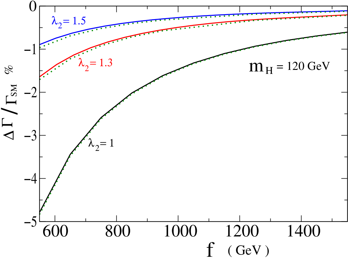
Figure 4: The variation in the top width. Solid lines contain the contribution from both the f1​Lf_{1L} and f2​Rf_{2R} couplings. Dotted lines are for f2​R=0f_{2R}=0.
Refer to caption
Figure 5: The variation in the W-boson helicity ratio f−f_{-}. It would require a deviation of f2​Rf_{2R} much bigger than 20%20\% in order to have a significant change in f−f_{-}.
t-channel: a0a_{0} ama_{m} apa_{p} a5a_{5} σtSM\sigma^{\rm SM}_{t}
Tevatron 0.995 -0.089 -0.181 0.336 0.906
LHC (tt) 174.2 -22.2 -38.1 78.2 151.99
LHC (t¯\bar{t}) 111.9 -23.4 -14.6 48.7 88.46
s-channel: b0b_{0} bmb_{m} bpb_{p} b5b_{5} σsSM\sigma^{\rm SM}_{s}
Tevatron -0.094 0.040 0.040 0.263 0.306
LHC (tt) -1.58 6.30 6.30 7.02 4.716
LHC (t¯\bar{t}) -0.944 3.83 3.83 3.76 2.884
Table 1: The single top production cross section coefficients of Eq. (90) for mt=173m_{t}=173 GeV. Last column is the Born level production cross section in the SM. All in units of pb.

As mentioned above, the LHT model predicts a tree level reduction of the t​b​WtbW coupling. Therefore, an important feature of this model is that at tree level all single top production modes as well as the total decay width show the same proportional deviation from the SM prediction[28]. In our study, we want to consider the additional effect from the dimension-5 f2​Rf_{2R} coupling that arises at the one loop level in LHT.

The SM born level prediction of the t→b​W+t\to bW^{+} width of the top quark is Γ⁡(t→b​W+)=1.5\Gamma(t\to bW^{+})=1.5 GeV for mt=173m_{t}=173 GeV. There is a 10%10\% decrease when QCD and electroweak corrections as well as non-zero mbm_{b} and finite W-boson width effects are considered[31, 27]. In Fig. (4) we show the deviation in the total width of the top quark coming from the LHT model. The solid lines in Fig. (4) give the reduction in Γt\Gamma_{t} as a funtion of the scale ff and three different values of λ2\lambda_{2}. For these lines both the effective f1​Lf_{1L} and f2​Rf_{2R} couplings are considered. Nonetheless, we also show in dotted lines the same curves obtained when only the f1​Lf_{1L} coupling is considered. Dotted and solid lines almost overlap: as expected, the change in Γt\Gamma_{t} is driven mainly by the tree level mixing with the heavy top. We conclude that the small changes in f2​Rf_{2R} cannot be seen by measuring Γt\Gamma_{t}. Also, notice that the (%\%) reduction in Fig. (4) is entirely due to the cosine of the t​TtT mixing angle cLc_{L}, which according to formula (75) tends to 1 when either ϵ→0\epsilon\to 0 or r=λ1/λ2→0r=\lambda_{1}/\lambda_{2}\to 0.

As for the W-boson helicity ratios f0f_{0} and f−f_{-}, in principle, these observables are more sensitive to the f2​Rf_{2R} coupling. Notice that L0L_{0} and TmT_{m} in equation (88) get exactly the same correction if only the f1​Lf_{1L} is modified (we have set f1​R=f2​L=0f_{1R}=f_{2L}=0). This means that the ratios f0f_{0} and f−f_{-} do not change at all from their SM values when we consider only the tree level t​b​WtbW coupling of the LHT model. However, when we consider the change in the f2​Rf_{2R} coupling we do observe a deviation that (unfortunately) turns out to be very small (of order less than 0.1%0.1\%) as it is shown in Fig. (5). We conclude that the W-boson helicity ratios f0f_{0} and f−f_{-} require a substantial deviation in the dimension five coupling f2​Rf_{2R} in order to show significant changes from their SM values.

Refer to caption
Figure 6: The variation in the σt\sigma_{t} cross section. Solid lines contain the contribution from both the f1​Lf_{1L} and f2​Rf_{2R} couplings. Dotted lines are for f2​R=0f_{2R}=0.

As mentioned above, the effective couplings f1​Lf_{1L} and f2​Rf_{2R} can also be probed with single top production. In comparison with the top decay width Γt\Gamma_{t} and the W-helicity ratio f−f_{-}, the cross section could be more sensitive to the f2​Rf_{2R} coupling. We show the deviation in the t-channel cross section in Fig. (6). Notice that the change when we go from considering the deviation in f1​Lf_{1L} only (dotted lines), to considering both the deviations in f1​Lf_{1L} and f2​Rf_{2R} (solid lines) is hardly visible. This change is slightly more pronounced for the s-channel cross section as shown in Fig. (7). We can observe from the values of the effective coefficients in Table (1) that for this channel the f2​Rf_{2R} coupling has a somewhat bigger effect through the x5x_{5} and x0x_{0} terms defined in equation (89). For instance, for a scale f=550f=550 GeV and λ2=1.5\lambda_{2}=1.5 the tree level f1​Lf_{1L} reduction expected in the LHT model brings about a 1.0%1.0\% reduction in σs\sigma_{s} (dotted line), whereas the combined f1​Lf_{1L} and f2​Rf_{2R} deviations bring a smaller 0.8%0.8\% reduction in σs\sigma_{s} (solid line). The reason for this can be seen in Fig. (2). The LHT contribution, on the one hand, decreases the value of f1​Lf_{1L}, and on the other hand increases the (positive) value of f2​Rf_{2R} with respect to the SM. We thus have a small compensation in the value of the xx terms in Eq. (89).

Refer to caption
Figure 7: The variation in the σs\sigma_{s} cross section. Solid lines contain the contribution from both the f1​Lf_{1L} and f2​Rf_{2R} couplings. Dotted lines are for f2​R=0f_{2R}=0.

IV Conclusions

Besides the SM electroweak parameters, the LHT model adds three more free parameters: κ\kappa, λ2\lambda_{2} and the scale ff (which is associated with an estimated cut-off Λ∼4​π​f\Lambda\sim 4\pi f). We have chosen a value of the mirror fermion yukawa κ=1\kappa=1 that for our range of ff gives T-odd fermion masses that are consistent with bounds from four fermion contact interactions e+​e−​q​q¯e^{+}e^{-}q\bar{q} and from unitarity in u​u¯→WH+​WH−u\bar{u}\to W^{+}_{H}W^{-}_{H} scattering processes. Our study concentrates on the two other parameters: λ2\lambda_{2} (which drives mT+m_{T^{+}}) and the scale ff. As for the values of λ2\lambda_{2} and ff we have chosen λ2=1\lambda_{2}=1, 1.31.3 and 1.51.5 and 550≤f≤1550550\leq f\leq 1550 GeV as suggested by Ref. [22].

Because of the mixing between the top quark and its heavy partner T+T^{+}, the LHT model predicts a tree level reduction of the dim 4 f1​Lf_{1L} coupling that implies an expected proportional reduction in the top width and single top production. Changes in f1​Lf_{1L} by themselves do not vary the predicted W helicity fractions in the t→b​Wt\to bW decay. However, the contribution from the f2​Rf_{2R} coupling could modify these fractions. The dim 5 weak dipole coupling f2​Rf_{2R} arises at the one loop level in the SM and in the LHT model. It is somewhat increased in size by the LHT model. However, the contribution to fmf_{m} (and f0f_{0}) is negligible. The increase in f2​Rf_{2R} predicted by the LHT tends to counteract the effects of the reduction in f1​Lf_{1L}. In any case, the effects from f2​Rf_{2R} are very small. We have found that the tree level analysis of the top’s width and the single top cross section remains valid for the LHT model. Top quark observables like total width, and single top production are sensitive to the mixing with the heavy T+T^{+} partner. In particular, the LHC may probe deviations of the f1​Lf_{1L} t​b​WtbW coupling down to a few percent[4] and this would imply an indirect probe of the scale ff (and the yukawa λ2\lambda_{2}) of the LHT model ( see Eq. (75) ). Of course, there are direct tests of the new heavy states at the LHC that will give more precise determination of these parameters. A recent study (see Ref. [22]) has shown that signal events from T+T^{+} and T−T^{-} production can be distinguished from SM backgrounds so that the mass and mixings of the top partners can be obtained with relatively good accuracies. Furthermore, other studies have shown that, since the mass of the T-odd fermions cannot be too heavy to be consistent with low energy data, they can be produced at high enough rates at the LHC[20].

Acknowledgments    We thank C.-P. Yuan, Chuan-Ren Chen, M.A. Pérez and R. Martinez for useful discussions. We thank Conacyt for support.

Appendix A The Goldstone boson sector in the ’t Hooft-Feynman gauge.

In the LHT model, the charged fields ω±\omega^{\pm} and ϕ±\phi^{\pm} as well as the neutral fields ω0\omega^{0}, η\eta and ϕP0\phi^{0}_{P}, mix at order (vf)2(\frac{v}{f})^{2}. It is a linear combination of these that is eaten by the heavy gauge bosons when the extended gauge group is broken down to S​U​(2)L×U​(1)YSU(2)_{L}\times U(1)_{Y}. On the other hand, the π\pi fields are T-parity even and do not mix with the other scalars. They are absorbed by the standard model W/ZW/Z bosons as usual. The fields hh, ϕ0\phi^{0}, ϕP0\phi^{0}_{P} and ϕ±\phi^{\pm} remain in the spectrum (after diagonalization). The basis of the kinetic Lagrangian of Eq. (19) is an exponential matrix that is usually computed up to the first few leading terms. However, it is possible to obtain the exact expressions for the kinetic (∂μϕ​∂μϕ\partial^{\mu}\phi\partial_{\mu}\phi) scalar, the scalar-boson mixing (Wμ+​∂μπ−W_{\mu}^{+}\partial^{\mu}\pi^{-}) and boson mass terms. (It is from the latter that the boson masses of Eq. (37) were obtained.)

In obtaining the following formulas it is convenient to notice that the vev value of the field matrix Π\Pi Eq. (II) is proportional to a matrix M0M_{0}:

M0=(0000000100010010000000100),\displaystyle M_{0}\,=\left(\begin{array}[]{ccccc}~0&~0&~0&~0&~0\\ 0&0&1&0&0\\ 0&1&0&0&1\\ 0&0&0&0&0\\ 0&0&1&0&0\end{array}\right),

for which is easy to prove that M02​n+1=2n​M0M_{0}^{2n+1}=2^{n}M_{0} and M02​(n+1)=2n​M02M_{0}^{2(n+1)}=2^{n}M_{0}^{2} with n=0,1,2,3,..n=0,1,2,3,... With these identities it can be shown that the vev of Σ\Sigma is[15]:

⟨Σ⟩0=(000100−1−cv2i2​sv01+cv20i2​svcv0i2​sv1000001+cv2i2​sv0−1−cv2),\displaystyle\langle\Sigma\rangle_{0}\,=\,\left(\begin{array}[]{ccccc}0&0&0&1&0\\ 0&-\frac{1-c_{v}}{2}&\frac{i}{\sqrt{2}}s_{v}&0&\frac{1+c_{v}}{2}\\ 0&\frac{i}{\sqrt{2}}s_{v}&c_{v}&0&\frac{i}{\sqrt{2}}s_{v}\\ 1&0&0&0&0\\ 0&\frac{1+c_{v}}{2}&\frac{i}{\sqrt{2}}s_{v}&0&-\frac{1-c_{v}}{2}\\ \end{array}\right),

where sv=sin⁡2​ϵs_{v}=\sin{\sqrt{2}\epsilon} and ϵ≡v/f\epsilon\equiv v/f as defined in Eq. 35. This expression can be used in the kinetic Lagrangian Eq. (19) to obtain the (exact) mixing and mass terms of the LHT model. The diagonalization and normalization of Goldstone boson fields has been discussed at order ϵ2\epsilon^{2} for the charged sector in Ref. [15] and for the neutral sector in Ref. [32]. Below, we will make the same analysis for charged and neutral bosons exactly (at all orders in ϵ\epsilon).

A.1 The charged W±W^{\pm} bosons.

Let us write down the part of the kinetic Lagrangian Eq. (19) that involves the charged bosons of the LHT model. It is convenient to put it in a matricial form:

ℒkin\displaystyle{\cal L}_{\rm kin} =\displaystyle= ∂μϕ+⁣+​∂μϕ−⁣−+ 2​κ~​∂μπ+​∂μπ−+f​g​1−cv2​y​(Wμ+​∂μπ−+Wμ−​∂μπ+)\displaystyle\partial^{\mu}\phi^{++}\partial_{\mu}\phi^{--}\;+\;2\tilde{\kappa}\;\partial^{\mu}\pi^{+}\partial_{\mu}\pi^{-}\;+\;fg\frac{1-c_{v}}{\sqrt{2}\;y}(W^{+}_{\mu}\partial^{\mu}\pi^{-}\;+\;W^{-}_{\mu}\partial^{\mu}\pi^{+})
+\displaystyle+ (∂μω−∂μϕ−)​B​(∂μω+∂μϕ+)+f​g​WH​μ+​(1+κ02i​1−κ02)​(∂μω−∂μϕ−)\displaystyle(\;\partial_{\mu}\omega^{-}\;\;\;\;\partial_{\mu}\phi^{-}\;)\;B\;\left(\begin{array}[]{c}\partial^{\mu}\omega^{+}\\ \partial^{\mu}\phi^{+}\end{array}\right)\;+\;fgW^{+}_{H\mu}(\;\frac{1+\kappa_{0}}{2}\;\;\;\;i\frac{1-\kappa_{0}}{2}\;)\;\left(\begin{array}[]{c}\partial^{\mu}\omega^{-}\\ \partial^{\mu}\phi^{-}\end{array}\right)
+\displaystyle+ f​g​WH​μ−​(1+κ02−i​1−κ02)​(∂μω+∂μϕ+)\displaystyle fgW^{-}_{H\mu}(\;\frac{1+\kappa_{0}}{2}\;\;\;\;-i\frac{1-\kappa_{0}}{2}\;)\;\left(\begin{array}[]{c}\partial^{\mu}\omega^{+}\\ \partial^{\mu}\phi^{+}\end{array}\right)

with

B\displaystyle B =\displaystyle= (12+κ~−i⁡(12−κ~)i⁡(12−κ~)12+κ~)\displaystyle\left(\begin{array}[]{cc}\frac{1}{2}+\tilde{\kappa}&-i(\frac{1}{2}-\tilde{\kappa})\\ i(\frac{1}{2}-\tilde{\kappa})&\frac{1}{2}+\tilde{\kappa}\end{array}\right)
κ0\displaystyle\kappa_{0} =\displaystyle= sv2​ϵ= 1−2​ϵ23!+4​ϵ45!−…\displaystyle\frac{s_{v}}{\sqrt{2}\epsilon}\;=\;1-\frac{2\epsilon^{2}}{3!}+\frac{4\epsilon^{4}}{5!}-...
κ~\displaystyle\tilde{\kappa} =\displaystyle= 1−cv2​ϵ2=12!−2​ϵ24!+4​ϵ46!−…\displaystyle\frac{1-c_{v}}{2\epsilon^{2}}\;=\;\frac{1}{2!}-\frac{2\epsilon^{2}}{4!}+\frac{4\epsilon^{4}}{6!}-... (114)

We then redefine the T-even charged scalar π±\pi^{\pm} as well as the T-odd ω±\omega^{\pm} and ϕ±\phi^{\pm} to diagonalize the Lagrangian. The new T-even π′⁣±\pi^{\prime\pm} field is given by:

π±\displaystyle\pi^{\pm} ≡\displaystyle\equiv ±i2​κ~​π′⁣±\displaystyle\;\frac{\pm\,i}{\sqrt{2\tilde{\kappa}}}\;\pi^{\prime\pm} (115)

An extra phase ii multiplies the π′⁣±\pi^{\prime\pm} field so that the W±​π′⁣±W^{\pm}\pi^{\prime\pm} mixing and the S​U​(2)SU(2) gauge-fixing terms become identical to the usual SM expressions[33]. The other two charged scalars are redefined as:

(ω+ϕ+)≡T⁡(i​ω′⁣+ϕ′⁣+),T=m^WH2​κ~+κ02​(2​κ~+κ0i⁡(1−κ0)​2​κ~i⁡(2​κ~−κ0)(1+κ0)​2​κ~)\displaystyle\left(\begin{array}[]{c}\omega^{+}\\ \phi^{+}\end{array}\right)\;\equiv\;\;T\;\left(\begin{array}[]{c}i\omega^{\prime+}\\ \phi^{\prime+}\end{array}\right)\;\;\;\;\;\;T\;=\;\frac{\hat{m}_{W_{H}}}{2\tilde{\kappa}+\kappa_{0}^{2}}\left(\begin{array}[]{cc}2\tilde{\kappa}+\kappa_{0}&i(1-\kappa_{0})\sqrt{2\tilde{\kappa}}\\ i(2\tilde{\kappa}-\kappa_{0})&(1+\kappa_{0})\sqrt{2\tilde{\kappa}}\end{array}\right)

where m^WH=MWHf​g=3+cv2\hat{m}_{W_{H}}=\frac{M_{W_{H}}}{fg}\;=\frac{\sqrt{3+c_{v}}}{2}. Notice that the new ω′⁣±\omega^{\prime\pm} field has an extra phase factor ±i\pm i that is convenient to use so that the Feynman rules of this T-odd Goldstone boson resemble the rules of its T-even counterpart (the π′⁣±\pi^{\prime\pm} boson). On the other hand, for the physical heavy T-odd ϕ′⁣±\phi^{\prime\pm} boson we choose not to insert the phase factor. The Feynman rules in appendix B stand for the new π′⁣±\pi^{\prime\pm}, ω′⁣±\omega^{\prime\pm}, ϕ′⁣±\phi^{\prime\pm}, etc. fields, but we have dropped the ′\prime symbol for simplicity.

In terms of the new (mass eigenstates) fields the Lagrangian becomes:

ℒkin\displaystyle{\cal L}_{\rm kin} =\displaystyle= ∂μϕ′⁣+​∂μϕ′⁣−\displaystyle\partial^{\mu}\phi^{\prime+}\partial_{\mu}\phi^{\prime-} (123)
+\displaystyle+ ∂μπ′⁣+​∂μπ′⁣−+i​MW​(Wμ−​∂μπ′⁣+−Wμ+​∂μπ′⁣−)\displaystyle\partial^{\mu}\pi^{\prime+}\partial_{\mu}\pi^{\prime-}\;+\;iM_{W}\left(W^{-}_{\mu}\partial^{\mu}\pi^{\prime+}-W^{+}_{\mu}\partial^{\mu}\pi^{\prime-}\right)
+\displaystyle+ ∂μω′⁣+​∂μω′⁣−+i​MWH​(WH​μ−​∂μω′⁣+−WH​μ+​∂μω′⁣−)\displaystyle\partial^{\mu}\omega^{\prime+}\partial_{\mu}\omega^{\prime-}\;+\;iM_{W_{H}}\left(W^{-}_{H\mu}\partial^{\mu}\omega^{\prime+}-W^{+}_{H\mu}\partial^{\mu}\omega^{\prime-}\right)

where the WH​μ+​∂μω′⁣−W^{+}_{H\mu}\partial^{\mu}\omega^{\prime-} mixing term is canceled (after integration by parts) when we add the usual gauge-fixing term:

Δ​ℒ=−1ξL​|∂μWμ±−i​MW​ξL​π′⁣±|2−1ξH​|∂μWH​μ±−i​MWH​ξH​ω′⁣±|2.\Delta{\cal L}=\frac{-1}{\xi_{L}}\left|\partial^{\mu}W_{\mu}^{\pm}-iM_{W}\xi_{L}\pi^{\prime\pm}\right|^{2}\;-\;\frac{1}{\xi_{H}}\left|\partial^{\mu}W_{H\mu}^{\pm}-iM_{W_{H}}\xi_{H}\omega^{\prime\pm}\right|^{2}. (124)

To obtain Feynman rules it is convenient to use an expansion in powers of ϵ=v/f\epsilon=v/f:

T= 1+(14​i2​i1)​ϵ224+(−61813​i192​i−1)​ϵ4720\displaystyle T\;=\;{\bf 1}\;+\;\left(\begin{array}[]{cc}1&4i\\ 2i&1\end{array}\right)\;\frac{\epsilon^{2}}{24}\;\;+\;\left(\begin{array}[]{cc}-\frac{61}{8}&13i\\ \frac{19}{2}i&-1\end{array}\right)\frac{\epsilon^{4}}{720}

A.2 The neutral bosons.

The neutral boson sector in the Lagrangian of Eq. (19) can also be written in the following matricial form (notice that MZ=v​g2​cw​2​κ~M_{Z}=\frac{vg}{2c_{w}}\sqrt{2\tilde{\kappa}}):

ℒkin\displaystyle{\cal L}_{\rm kin} =\displaystyle= 12​(∂μh)2+κ~​(∂μϕ0)2+κ~​(∂μπ0)2+v​gcw​κ~​Zμ​∂μπ0\displaystyle\frac{1}{2}(\partial^{\mu}h)^{2}\;+\;\tilde{\kappa}(\partial^{\mu}\phi^{0})^{2}\;+\;\tilde{\kappa}(\partial^{\mu}\pi^{0})^{2}\;+\;\frac{vg}{c_{w}}\tilde{\kappa}\;Z^{\mu}\partial_{\mu}\pi^{0} (130)
+\displaystyle+ x¯T​A​x¯+AHμ​a¯T​x¯+ZHμ​b¯T​x¯\displaystyle\bar{x}^{T}\,A\;\bar{x}\;+\;A_{H}^{\mu}\;\bar{a}^{T}\bar{x}\;+\;Z_{H}^{\mu}\;\bar{b}^{T}\bar{x}

with

x¯=(∂μω0∂μη∂μϕP0)​a¯\displaystyle\bar{x}\;=\;\left(\begin{array}[]{c}\partial_{\mu}\omega^{0}\\ \partial_{\mu}\eta\\ \partial_{\mu}\phi^{0}_{P}\end{array}\right)\;\;\;\bar{a} =\displaystyle= f​g​cH8​(8​tw−(4​κ1+κ2)​xω(8​tw−5​κ1​xω)/52​κ1​xω)​b¯=f​g​cH8​(8−κ1​xη(8−κ2​xη)/5−2​κ1​xη)\displaystyle\frac{fgc_{H}}{8}\left(\begin{array}[]{c}8t_{w}-(4\kappa_{1}+\kappa_{2})x_{\omega}\\ (8t_{w}-5\kappa_{1}x_{\omega})/{\sqrt{5}}\\ \sqrt{2}\kappa_{1}x_{\omega}\end{array}\right)\;\;\;\bar{b}\;=\;\frac{fgc_{H}}{8}\left(\begin{array}[]{c}8-\kappa_{1}x_{\eta}\\ (8-\kappa_{2}x_{\eta})/{\sqrt{5}}\\ -\sqrt{2}\kappa_{1}x_{\eta}\end{array}\right)
A\displaystyle A =\displaystyle= 116​(7+κ025​(1−κ02)−2​(1−κ02)5​(1−κ02)3+5​κ0210​(1−κ02)−2​(1−κ02)10​(1−κ02)6+2​κ02)\displaystyle\frac{1}{16}\;\left(\begin{array}[]{ccc}7+\kappa_{0}^{2}&\sqrt{5}(1-\kappa_{0}^{2})&-\sqrt{2}(1-\kappa_{0}^{2})\\ \sqrt{5}(1-\kappa_{0}^{2})&3+5\kappa_{0}^{2}&\sqrt{10}(1-\kappa_{0}^{2})\\ -\sqrt{2}(1-\kappa_{0}^{2})&\sqrt{10}(1-\kappa_{0}^{2})&6+2\kappa_{0}^{2}\end{array}\right)

and

κ1= 1−κ0​cv\displaystyle\kappa_{1}\;=\;1-\kappa_{0}c_{v}\;\;\;\;\;\;\;\;\;\;\;\;\;\;\;\;\;\;\;\;\;\;\;\;\; κ2= 3+5​κ0​cv\displaystyle\kappa_{2}\;=\;3+5\kappa_{0}c_{v}
xω=tw+tH\displaystyle x_{\omega}\;=\;t_{w}+t_{H}\;\;\;\;\;\;\;\;\;\;\;\;\;\;\;\;\;\;\;\;\;\;\; xη= 1−tw​tH\displaystyle x_{\eta}\;=\;1-t_{w}t_{H}
yω=tw−5​tH\displaystyle y_{\omega}\;=\;t_{w}-5t_{H}\;\;\;\;\;\;\;\;\;\;\;\;\;\;\;\;\;\;\;\;\;\;\; yη= 5+tw​tH\displaystyle y_{\eta}\;=\;5+t_{w}t_{H} (145)

Where tw≡sw/cwt_{w}\equiv s_{w}/c_{w} and tHt_{H} are Tan(θw\theta_{w}) and Tan(θH\theta_{H}) respectively ( see Eq. (34) ). To normalize the π0\pi^{0} and ϕ0\phi^{0} fields we simply redefine π′0≡2​κ~​π0\pi^{\prime 0}\equiv\sqrt{2\tilde{\kappa}}\pi^{0} and ϕ′0≡2​κ~​ϕ0\phi^{\prime 0}\equiv\sqrt{2\tilde{\kappa}}\phi^{0}. (The Higgs field hh needs no redefinition.) We also redefine the other scalars to properly diagonalize the Lagrangian:

(ω0ηϕP0)≡T⁡(ω′0η′ϕP′0)with​T=1κ0​2​1+3​cv2​D1​(ti​j)​D2\displaystyle\left(\begin{array}[]{c}\omega^{0}\\ \eta\\ \phi^{0}_{P}\end{array}\right)\;\equiv\;\;T\;\left(\begin{array}[]{c}\omega^{\prime 0}\\ \eta^{\prime}\\ \phi^{\prime 0}_{P}\end{array}\right)\;\;\;\;\;{\rm with}\;T\;=\;\frac{1}{\kappa_{0}\sqrt{2}\sqrt{1+3c^{2}_{v}}}\;D_{1}\;\left(\;t_{ij}\;\right)\;D_{2}

where TT is conveniently written as a product of 3 matrices: D1D_{1}, (ti​j)(t_{ij}) and D2D_{2}. Two of them are diagonal matrices defined as D1=d​i​a​g​(1,5,2)D_{1}=diag(1,\sqrt{5},\sqrt{2}), and D2=d​i​a​g​(1/dω,1/dη,1/2)D_{2}=diag(1/d_{\omega},1/d_{\eta},1/2), with

dω\displaystyle d_{\omega} =\displaystyle= 8​(tw2+5​tH2)−5​sv2​xω2,and\displaystyle\sqrt{8(t^{2}_{w}+5t^{2}_{H})-5s^{2}_{v}x^{2}_{\omega}}\;,\;{\rm and}
dη\displaystyle d_{\eta} =\displaystyle= 8​(5+tw2​tH2)−5​sv2​xη2.\displaystyle\sqrt{8(5+t^{2}_{w}t^{2}_{H})-5s^{2}_{v}x^{2}_{\eta}}\;.

The matrix elements ti​jt_{ij} are as follows:

t11=κ0​(5​cv2​xω+2​tw)+cv​yω\displaystyle t_{11}\;=\;\kappa_{0}(5c^{2}_{v}x_{\omega}+2t_{w})+c_{v}y_{\omega}\;\;\;\;\; t12=κ0​(5​cv2​xη−2​tw​tH)−cv​yηt13=κ1\displaystyle t_{12}\;=\;\kappa_{0}(5c^{2}_{v}x_{\eta}-2t_{w}t_{H})-c_{v}y_{\eta}\;\;\;\;\;\;\;\;t_{13}\;=\;\kappa_{1}
t21=κ0​(cv2​xω+2​tH)−cv​yω\displaystyle t_{21}\;=\;\kappa_{0}(c^{2}_{v}x_{\omega}+2t_{H})-c_{v}y_{\omega}\;\;\;\;\;\;\; t22=κ0​(cv2​xη+2)+cv​yηt23=−κ1\displaystyle t_{22}\;=\;\kappa_{0}(c^{2}_{v}x_{\eta}+2)+c_{v}y_{\eta}\;\;\;\;\;\;\;\;\;\;\;\;\;\;\;\;\;t_{23}\;=\;-\kappa_{1}
t31=−(κ0−cv)​yω\displaystyle t_{31}\;=\;-(\kappa_{0}-c_{v})y_{\omega}\;\;\;\;\;\;\;\;\;\;\;\;\;\;\;\;\;\;\;\; t32=(κ0−cv)​yηt33= 1+3​κ0​cv\displaystyle t_{32}\;=\;(\kappa_{0}-c_{v})y_{\eta}\;\;\;\;\;\;\;\;\;\;\;\;\;\;\;\;\;\;\;\;\;\;\;\;\;\;\;\;\;t_{33}\;=\;1+3\kappa_{0}c_{v}

where the xx’s, yy’s and κ\kappa’s are defined in equations (114) and (145).

It is convenient to make an expansion in powers of ϵ=v/f\epsilon=v/f:

T= 1+T2ϵ212+T4ϵ46+⋅⋅\displaystyle T\;=\;{\bf 1}\;+\;T_{2}\frac{\epsilon^{2}}{12}\;+\;T_{4}\frac{\epsilon^{4}}{6}\;+\;\cdot\cdot\;\;\;\;\;\;\;\;\;\;\;\;\;\;\;\;\;\;\;\;\;\;\;\;
T2=(1/2−2.183​52​22.1832​55/2−2​10−2101)​T4=(−0.56820.62004130​20.1315−0.6093−416​10−0.12881.6184−17240)\displaystyle T_{2}=\left(\begin{array}[]{ccc}1/2&-2.183\sqrt{5}&2\sqrt{2}\\ \frac{2.183}{2}\sqrt{5}&5/2&-2\sqrt{10}\\ -\sqrt{2}&\sqrt{10}&1\end{array}\right)\;\;\;T_{4}=\left(\begin{array}[]{ccc}-0.5682&0.6200&\frac{41}{30\sqrt{2}}\\ 0.1315&-0.6093&\frac{-41}{6\sqrt{10}}\\ -0.1288&1.6184&\frac{-17}{240}\end{array}\right)

where we have taken tw=0.536t_{w}=0.536, thus (10+tw2)/(5−tw2)=2.183(10+t^{2}_{w})/(5-t^{2}_{w})\,=2.183.

In terms of the new (mass eigenstates) fields the neutral boson Lagrangian becomes:

ℒkin\displaystyle{\cal L}_{\rm kin} =\displaystyle= 12​(∂μh)2+12​(∂μπ′0)2+MZ​Zμ​∂μπ′0\displaystyle\frac{1}{2}(\partial^{\mu}h)^{2}\;+\;\frac{1}{2}(\partial^{\mu}\pi^{\prime 0})^{2}\;+\;M_{Z}Z^{\mu}\partial_{\mu}\pi^{\prime 0} (160)
+\displaystyle+ 12​(∂μω′0)2+12​(∂μη′)2+12​(∂μϕP′0)2+12​(∂μϕ′0)2\displaystyle\frac{1}{2}(\partial^{\mu}\omega^{\prime 0})^{2}\;+\;\frac{1}{2}(\partial^{\mu}\eta^{\prime})^{2}\;+\;\frac{1}{2}(\partial^{\mu}\phi_{P}^{\prime 0})^{2}\;+\;\frac{1}{2}(\partial^{\mu}\phi^{\prime 0})^{2}
+\displaystyle+ MZH​ZHμ​∂μω′0+MAH​AHμ​∂μη′\displaystyle M_{Z_{H}}Z_{H}^{\mu}\partial_{\mu}\omega^{\prime 0}\;+\;M_{A_{H}}A_{H}^{\mu}\partial_{\mu}\eta^{\prime}

where the mixing terms like Zμ​∂μπ′0Z^{\mu}\partial_{\mu}\pi^{\prime 0} are canceled (after integration by parts) when we add the usual gauge-fixing terms:

Δ​ℒ\displaystyle\Delta{\cal L} =\displaystyle= −12​ξA​(∂μAμ)2−12​ξZ​(∂μZμ−MZ​ξZ​π′0)2\displaystyle\frac{-1}{2\xi_{A}}\left(\partial_{\mu}A^{\mu}\right)^{2}\;-\;\frac{1}{2\xi_{Z}}\left(\partial_{\mu}Z^{\mu}-M_{Z}\xi_{Z}\pi^{\prime 0}\right)^{2} (161)
−\displaystyle- 12​ξAH​(∂μAHμ−MAH​ξAH​η′)2−12​ξZH​(∂μZHμ−MZH​ξZH​ω′0)2\displaystyle\frac{1}{2\xi_{A_{H}}}\left(\partial_{\mu}A_{H}^{\mu}-M_{A_{H}}\xi_{A_{H}}\eta^{\prime}\right)^{2}\;-\;\frac{1}{2\xi_{Z_{H}}}\left(\partial_{\mu}Z_{H}^{\mu}-M_{Z_{H}}\xi_{Z_{H}}\omega^{\prime 0}\right)^{2}

Appendix B Feynman rules.

We want to show the Feynamn rules that we used. The scalar fields are not the original interaction eigenstates but the mass eigenstates that are written as π′⁣±\pi^{\prime\pm}, π′0\pi^{\prime 0}, etc. We have dropped the ′\prime symbol to simplify the notation. Table 2 shows bosonic vertices that involve one charged W−W^{-} SM boson. Tables 3, 4 and 5 show vertices for fermions and charged, T-even neutral and T-odd neutral scalar bosons respectively. For the fermion-gauge boson interactions we refer the reader to tables V and VI of Ref. [20]. We have carefully verified that our rules agree with the ones there. We have written in Table 6 some others that do not appear in [20]. Other types of interactions, like four-boson vertices or dimension-5 f¯​f​ϕ​ϕ\bar{f}f\phi\phi (ϕ\phi any scalar) vertices can be found in Ref. [21].

Please notice the definitions (ϵ=v/f\epsilon=v/f, r=λ1/λ2r=\lambda_{1}/\lambda_{2}):

Sλ​ν​μ\displaystyle S_{\lambda\nu\mu} ≡\displaystyle\equiv (p−−p+)λ​gμ​ν+(p+−p0)μ​gν​λ+(p0−p−)ν​gλ​μ\displaystyle(p_{-}-p_{+})_{\lambda}g_{\mu\nu}\,+\,(p_{+}-p_{0})_{\mu}g_{\nu\lambda}\,+\,(p_{0}-p_{-})_{\nu}g_{\lambda\mu}\,
qw\displaystyle q_{w} ≡\displaystyle\equiv 10+tw25−tw2\displaystyle\frac{10+t_{w}^{2}}{5-t_{w}^{2}}
Interaction      Feynman rule Interaction      Feynman rule
Wμ−​Wν+​AλW_{\mu}^{-}W_{\nu}^{+}A_{\lambda} i​g​sw​Sλ​ν​μig\,s_{w}\,S_{\lambda\nu\mu} Wμ−​WH​ν+​ϕP0W_{\mu}^{-}W_{H\nu}^{+}\phi^{0}_{P} ∼ϵ4\sim\epsilon^{4}
Wμ−​Wν+​ZλW_{\mu}^{-}W_{\nu}^{+}Z_{\lambda} i​g​cw​Sλ​ν​μig\,c_{w}\,S_{\lambda\nu\mu} Wμ−​ω+​AH​νW_{\mu}^{-}\omega^{+}A_{H\nu} i​g2​f​tw​(520−4​tW2−14)​ϵ2​gμ​νig^{2}\,f\,t_{w}(\frac{5}{20-4t_{W}^{2}}-\frac{1}{4})\epsilon^{2}\,g_{\mu\nu}
Wμ−​π+​AνW_{\mu}^{-}\pi^{+}A_{\nu} i​g​sw​MW​(1−112​ϵ2)​gμ​νig\,s_{w}M_{W}(1-\frac{1}{12}\epsilon^{2})g_{\mu\nu} Wμ−​ω+​ZH​νW_{\mu}^{-}\omega^{+}Z_{H\nu} −i​g2​f​(1−38​ϵ2)​gμ​ν-ig^{2}\,f(1-\frac{3}{8}\epsilon^{2})g_{\mu\nu}
Wμ−​π+​ZνW_{\mu}^{-}\pi^{+}Z_{\nu} −i​g​sw2​MZ​(1−112​ϵ2)​gμ​ν-ig\,s_{w}^{2}M_{Z}(1-\frac{1}{12}\epsilon^{2})g_{\mu\nu} Wμ−​ϕ+​AH​νW_{\mu}^{-}\phi^{+}A_{H\nu} g2​tw4​f​ϵ2​gμ​νg^{2}\frac{t_{w}}{4}f\epsilon^{2}g_{\mu\nu}
Wμ−​Wν+​hW_{\mu}^{-}W_{\nu}^{+}h i​g​MW​(1−13​ϵ2)​gμ​νig\,M_{W}(1-\frac{1}{3}\epsilon^{2})g_{\mu\nu} Wμ−​ϕ+​ZH​νW_{\mu}^{-}\phi^{+}Z_{H\nu} i​g2​f4​(23+53​i)​ϵ2​gμ​νig^{2}\,\frac{f}{4}(\frac{2}{3}+\frac{5}{3}i)\epsilon^{2}g_{\mu\nu}
Wμ−​Wν+​π0W_{\mu}^{-}W_{\nu}^{+}\pi^{0} 00 Wμ−​ω+​ω0W_{\mu}^{-}\omega^{+}\omega^{0} g⁡(1−18​ϵ2)​(pω+​μ−p0​μ)g(1-\frac{1}{8}\epsilon^{2})(p_{\omega^{+}\mu}-p_{0\mu})
Wμ−​π+​hW_{\mu}^{-}\pi^{+}h i​g2​[pπ​μ​(1−512​ϵ2)−ph​μ​(1−112​ϵ2)]i\frac{g}{2}[p_{\pi\mu}(1-\frac{5}{12}\epsilon^{2})-p_{h\mu}(1-\frac{1}{12}\epsilon^{2})] Wμ−​ω+​ηW_{\mu}^{-}\omega^{+}\eta g​512​ϵ2​[(qw−32)​pη​μ−(qw+12)​pω+​μ]g\frac{\sqrt{5}}{12}\epsilon^{2}[(q_{w}-\frac{3}{2})p_{\eta\mu}-(q_{w}+\frac{1}{2})p_{\omega^{+}\mu}]
Wμ−​π+​π0W_{\mu}^{-}\pi^{+}\pi^{0} g2​(pπ+​μ−p0​μ)\frac{g}{2}(p_{\pi^{+}\mu}-p_{0\mu}) Wμ−​ω+​ϕ0W_{\mu}^{-}\omega^{+}\phi^{0} −g12​2​ϵ2​[(1+2​i)​pϕ​μ−pω​μ]-\frac{g}{12\sqrt{2}}\epsilon^{2}[(1+2i)p_{\phi\mu}-p_{\omega\mu}]
Wμ−​WH​ν+​AH​λW_{\mu}^{-}W_{H\nu}^{+}A_{H\lambda} −i​g​sh​Sλ​ν​μ-ig\,s_{h}\,S_{\lambda\nu\mu} Wμ−​ω+​ϕP0W_{\mu}^{-}\omega^{+}\phi^{0}_{P} i​g​2​112​ϵ2​[12​pϕ​μ−(12+i)​pω​μ]ig\sqrt{2}\frac{1}{12}\epsilon^{2}[\frac{1}{2}p_{\phi\mu}-(\frac{1}{2}+i)p_{\omega\mu}]
Wμ−​WH​ν+​ZH​λW_{\mu}^{-}W_{H\nu}^{+}Z_{H\lambda} i​g​ch​Sλ​ν​μig\,c_{h}\,S_{\lambda\nu\mu} Wμ−​ϕ+​ω0W_{\mu}^{-}\phi^{+}\omega^{0} −g6​(1+74​i)​(pϕ+​μ−pω0​μ)​ϵ2-\frac{g}{6}(1+\frac{7}{4}i)(p_{\phi^{+}\mu}-p_{\omega_{0}\mu})\epsilon^{2}
Wμ−​WH​ν+​ηW_{\mu}^{-}W_{H\nu}^{+}\eta 52​g2​f​(1+qw)​ϵ2​gμ​ν\frac{\sqrt{5}}{2}g^{2}f(1+q_{w})\epsilon^{2}\,g_{\mu\nu} Wμ−​ϕ+​ηW_{\mu}^{-}\phi^{+}\eta −i​g​512​(52​pη​μ−12​pϕ+​μ)​ϵ2-ig\frac{\sqrt{5}}{12}(\frac{5}{2}p_{\eta\mu}-\frac{1}{2}p_{\phi^{+}\mu})\epsilon^{2}
Wμ−​WH​ν+​ϕ0W_{\mu}^{-}W_{H\nu}^{+}\phi^{0} 0 Wμ−​ϕ+​ϕ0W_{\mu}^{-}\phi^{+}\phi^{0} g2​[p0​μ−pϕ+​μ−124​ϵ2​(5​p0​μ−pϕ+​μ)]\frac{g}{\sqrt{2}}[p_{0\mu}-p_{\phi^{+}\mu}-\frac{1}{24}\epsilon^{2}(5p_{0\mu}-p_{\phi^{+}\mu})]
Wμ−​WH​ν+​ω0W_{\mu}^{-}W_{H\nu}^{+}\omega^{0} g2​f​(1−38​ϵ2)​gμ​νg^{2}f(1-\frac{3}{8}\epsilon^{2})g_{\mu\nu} Wμ−​ϕ+​ϕP0W_{\mu}^{-}\phi^{+}\phi^{0}_{P} −i​g2​[pϕ0​μ−pϕ+​μ−124​(5​pϕ0​μ−pϕ+​μ)​ϵ2]-i\frac{g}{\sqrt{2}}[p_{\phi^{0}\mu}-p_{\phi^{+}\mu}-\frac{1}{24}(5p_{\phi^{0}\mu}-p_{\phi^{+}\mu})\epsilon^{2}]
Table 2: Feynman rules for three boson W−W^{-} vertices. Some of these rules also appear in Ref. [32]. Here, MWM_{W} and MZM_{Z} stand for the SM mass of the W±W^{\pm} and ZZ bosons.
AR\displaystyle A_{R} ≡\displaystyle\equiv i​2​λd​[−1+r42​(1+r2)2​ϵ2]\displaystyle i\sqrt{2}\lambda_{d}\left[-1+\frac{r^{4}}{2(1+r^{2})^{2}}\epsilon^{2}\right]
AL\displaystyle A_{L} ≡\displaystyle\equiv i​2​λ2​r1+r2​[1−1+3​r44​(1+r2)2​ϵ2]\displaystyle i\frac{\sqrt{2}\lambda_{2}r}{\sqrt{1+r^{2}}}\left[1-\frac{1+3r^{4}}{4(1+r^{2})^{2}}\epsilon^{2}\right]
BR\displaystyle B_{R} ≡\displaystyle\equiv i​2​λd​r21+r2​[−ϵ+5−2​r2+2​r46​(1+r2)2​ϵ3]\displaystyle i\frac{\sqrt{2}\lambda_{d}\,r^{2}}{1+r^{2}}\left[-\epsilon+\frac{5-2r^{2}+2r^{4}}{6(1+r^{2})^{2}}\epsilon^{3}\right]
BL\displaystyle B_{L} ≡\displaystyle\equiv i​2​λ2​r21+r2​[1−ϵ24​3+r4(1+r2)2]\displaystyle i\sqrt{2}\lambda_{2}\frac{r^{2}}{\sqrt{1+r^{2}}}\left[1-\frac{\epsilon^{2}}{4}\frac{3+r^{4}}{(1+r^{2})^{2}}\right]
DR\displaystyle D_{R} ≡\displaystyle\equiv (i+4)​κ​ϵ224\displaystyle(i+4)\kappa\frac{\epsilon^{2}}{24}
DL\displaystyle D_{L} ≡\displaystyle\equiv i​r​λ22​1+r2​[−ϵ+ϵ324​7−4​i+(2−8​i)​r2+(19−4​i)​r4(1+r2)2]\displaystyle\frac{ir\lambda_{2}}{\sqrt{2}\sqrt{1+r^{2}}}\left[-\epsilon+\frac{\epsilon^{3}}{24}\frac{7-4i+(2-8i)r^{2}+(19-4i)r^{4}}{(1+r^{2})^{2}}\right]
EL\displaystyle E_{L} ≡\displaystyle\equiv i​r2​λ22​(1+r2)​[−ϵ+19+4​i+(2+8​i)​r2+(7+4​i)​r424​(1+r2)2​ϵ3]\displaystyle\frac{ir^{2}\lambda_{2}}{\sqrt{2(1+r^{2})}}\left[-\epsilon+\frac{19+4i+(2+8i)r^{2}+(7+4i)r^{4}}{24(1+r^{2})^{2}}\epsilon^{3}\right]
aR\displaystyle a_{R} ≡\displaystyle\equiv −κ⁡[1−r4​ϵ22​(1+r2)2]\displaystyle-\kappa\left[1-\frac{r^{4}\epsilon^{2}}{2(1+r^{2})^{2}}\right]
aL\displaystyle a_{L} ≡\displaystyle\equiv r​λ22​1+r2​(ϵ−i​ϵ3​[2−7​i+(4−2​i)​r2+(2−19​i)​r4]24​(1+r2)2)\displaystyle\frac{r\lambda_{2}}{\sqrt{2}\sqrt{1+r^{2}}}\left(\epsilon-\frac{i\epsilon^{3}[2-7i+(4-2i)r^{2}+(2-19i)r^{4}]}{24(1+r^{2})^{2}}\right)
bR\displaystyle b_{R} ≡\displaystyle\equiv r2​κ1+r2​[−ϵ+5−2​r2+2​r46​(1+r2)2​ϵ3]\displaystyle\frac{r^{2}\kappa}{1+r^{2}}\left[-\epsilon+\frac{5-2r^{2}+2r^{4}}{6(1+r^{2})^{2}}\epsilon^{3}\right]
bL\displaystyle b_{L} ≡\displaystyle\equiv r2​λ22​(1+r2)​[ϵ−19+2​i+(2+4​i)​r2+(7+2​i)​r424​(1+r2)2​ϵ3]\displaystyle\frac{r^{2}\lambda_{2}}{\sqrt{2(1+r^{2})}}\left[\epsilon-\frac{19+2i+(2+4i)r^{2}+(7+2i)r^{4}}{24(1+r^{2})^{2}}\epsilon^{3}\right]
Interaction      Feynman rule Interaction      Feynman rule
t¯+​b+​π+\bar{t}^{+}b^{+}\pi^{+} AR​PR+AL​PLA_{R}P_{R}+A_{L}P_{L} t¯−​b+​ω+\bar{t}^{-}b^{+}\omega^{+} i​λd2​[−ϵ+(1−2​i)​124​ϵ3]​PR+i​κ​PLi\frac{\lambda_{d}}{\sqrt{2}}[-\epsilon+(1-2i)\frac{1}{24}\epsilon^{3}]P_{R}+i\kappa P_{L}
T¯+​b+​π+\bar{T}^{+}b^{+}\pi^{+} BR​PR+BL​PLB_{R}P_{R}+B_{L}P_{L} T¯−​b+​ω+\bar{T}^{-}b^{+}\omega^{+} 00
t¯−​b−​π+\bar{t}^{-}b^{-}\pi^{+} −i​κ4​(ϵ+124​ϵ3)​γ5-i\frac{\kappa}{4}(\epsilon+\frac{1}{24}\epsilon^{3})\gamma_{5} t¯+​b−​ϕ+\bar{t}^{+}b^{-}\phi^{+} DR​PR+DL​PLD_{R}\,P_{R}+D_{L}\,P_{L}
T¯−​b−​π+\bar{T}^{-}b^{-}\pi^{+} 00 T¯+​b−​ϕ+\bar{T}^{+}b^{-}\phi^{+} i​r2​κ24​(1+r2)​[1−4​i]​ϵ3​PR+EL​PLi\frac{r^{2}\kappa}{24(1+r^{2})}[1-4i]\epsilon^{3}P_{R}+E_{L}P_{L}
t¯+​b−​ω+\bar{t}^{+}b^{-}\omega^{+} i⁡[aR​PR+aL​PL]i[a_{R}\,P_{R}+a_{L}\,P_{L}] t¯−​b+​ϕ+\bar{t}^{-}b^{+}\phi^{+} i​λd2​[ϵ−(1+4​i)24​ϵ3]​PR−i⁡(4​i+1)​κ24​ϵ2​PLi\frac{\lambda_{d}}{\sqrt{2}}[\epsilon-\frac{(1+4i)}{24}\epsilon^{3}]P_{R}-i(4i+1)\frac{\kappa}{24}\epsilon^{2}P_{L}
T¯+​b−​ω+\bar{T}^{+}b^{-}\omega^{+} i⁡[bR​PR+bL​PL]i[b_{R}P_{R}+b_{L}P_{L}] T¯−​b+​ϕ+\bar{T}^{-}b^{+}\phi^{+} 00
Table 3: Feynman rules for fermion-charged scalar vertices.
GR\displaystyle G_{R} ≡\displaystyle\equiv 1r⁡(1+r2)​[ϵ+3​r6−2​r4+8​r2−26​(1+r2)2​ϵ3]\displaystyle\frac{1}{r(1+r^{2})}\left[\epsilon+\frac{3r^{6}-2r^{4}+8r^{2}-2}{6(1+r^{2})^{2}}\epsilon^{3}\right]
GL\displaystyle G_{L} ≡\displaystyle\equiv −1+3+r2+r42​(1+r2)2​ϵ2\displaystyle-1+\frac{3+r^{2}+r^{4}}{2(1+r^{2})^{2}}\epsilon^{2}
JR\displaystyle J_{R} ≡\displaystyle\equiv r1+r2​[ϵ−ϵ3​(13−4​r2+13​r4)12​(1+r2)2]\displaystyle\frac{r}{1+r^{2}}\left[\epsilon-\frac{\epsilon^{3}(13-4r^{2}+13r^{4})}{12(1+r^{2})^{2}}\right]
JL\displaystyle J_{L} ≡\displaystyle\equiv 3​ϵ2​(1+r4)4​(1+r2)2−1\displaystyle\frac{3\epsilon^{2}(1+r^{4})}{4(1+r^{2})^{2}}-1
Interaction      Feynman rule Interaction      Feynman rule
t¯+​t+​h\bar{t}^{+}t^{+}h i​r​λ21+r2​(−1+2+r2+2​r42​(1+r2)2​ϵ2)i\frac{r\lambda_{2}}{\sqrt{1+r^{2}}}(-1+\frac{2+r^{2}+2r^{4}}{2(1+r^{2})^{2}}\epsilon^{2}) t¯+​t+​π0\bar{t}^{+}t^{+}\pi^{0} −r​λ21+r2​[1−(1+5​r4)4​(1+r2)2​ϵ2]​γ5-\frac{r\lambda_{2}}{\sqrt{1+r^{2}}}[1-\frac{(1+5r^{4})}{4(1+r^{2})^{2}}\epsilon^{2}]\gamma_{5}
T¯+​T+​h\bar{T}^{+}T^{+}h i​λ2​[r2(r2+1)3/2​ϵ+r2​(3​r6+r4+8​r2−5)6​(r2+1)7/2​ϵ3]i\lambda_{2}[\frac{r^{2}}{\left(r^{2}+1\right)^{3/2}}\epsilon+\frac{r^{2}\left(3r^{6}+r^{4}+8r^{2}-5\right)}{6\left(r^{2}+1\right)^{7/2}}\epsilon^{3}] T¯+​T+​π0\bar{T}^{+}T^{+}\pi^{0} r4​λ2(1+r2)32​[−ϵ+19−4​r2+7​r412​(1+r2)2​ϵ3]​γ5\frac{r^{4}\lambda_{2}}{(1+r^{2})^{\frac{3}{2}}}[-\epsilon+\frac{19-4r^{2}+7r^{4}}{12(1+r^{2})^{2}}\epsilon^{3}]\gamma_{5}
T¯+​t+​h\bar{T}^{+}t^{+}h i​r2​λ21+r2​(GR​PR+GL​PL)i\frac{r^{2}\lambda_{2}}{\sqrt{1+r^{2}}}(G_{R}\,P_{R}+G_{L}\,P_{L}) T¯+​t+​π0\bar{T}^{+}t^{+}\pi^{0} −r2​λ21+r2​(JR​PR+JL​PL)-\frac{r^{2}\lambda_{2}}{\sqrt{1+r^{2}}}(J_{R}P_{R}+J_{L}P_{L})
b¯+​b+​h\bar{b}^{+}b^{+}h i​λd​(−1+34​ϵ2)i\lambda_{d}(-1+\frac{3}{4}\epsilon^{2}) b¯+​b+​π0\bar{b}^{+}b^{+}\pi^{0} λd​γ5\lambda_{d}\,\gamma_{5}
t¯−​t−​h\bar{t}^{-}t^{-}h 00 t¯−​t−​π0\bar{t}^{-}t^{-}\pi^{0} −κ2​2​(ϵ+124​ϵ3)​γ5-\frac{\kappa}{2\sqrt{2}}(\epsilon+\frac{1}{24}\epsilon^{3})\gamma_{5}
T¯−​T−​h\bar{T}^{-}T^{-}h 00 T¯−​T−​π0\bar{T}^{-}T^{-}\pi^{0} 00
T¯−​t−​h\bar{T}^{-}t^{-}h 00 T¯−​t−​π0\bar{T}^{-}t^{-}\pi^{0} 00
b¯−​b−​h\bar{b}^{-}b^{-}h 00 b¯−​b−​π0\bar{b}^{-}b^{-}\pi^{0} 00
Table 4: Feynman rules for fermion-neutral T-even scalar vertices.
KR\displaystyle K_{R} ≡\displaystyle\equiv −κ2​[1−(1+qw+12​r4(1+r2)2)​ϵ224]\displaystyle-\frac{\kappa}{\sqrt{2}}\left[1-\left(1+q_{w}+\frac{12r^{4}}{(1+r^{2})^{2}}\right)\frac{\epsilon^{2}}{24}\right]
KL\displaystyle K_{L} ≡\displaystyle\equiv r​λ22​1+r2​[ϵ−(qw+3−6​r2+15​r4(1+r2)2)​ϵ324]\displaystyle\frac{r\lambda_{2}}{2\sqrt{1+r^{2}}}\left[\epsilon-\left(q_{w}+\frac{3-6r^{2}+15r^{4}}{(1+r^{2})^{2}}\right)\frac{\epsilon^{3}}{24}\right]
MR\displaystyle M_{R} ≡\displaystyle\equiv r2​κ2​(1+r2)​(−ϵ+[qw+21−6​r2+9​r4(1+r2)2]​124​ϵ3)\displaystyle\frac{r^{2}\kappa}{\sqrt{2}(1+r^{2})}\left(-\epsilon+\left[q_{w}+\frac{21-6r^{2}+9r^{4}}{(1+r^{2})^{2}}\right]\frac{1}{24}\epsilon^{3}\right)
ML\displaystyle M_{L} ≡\displaystyle\equiv r2​λ22​1+r2​(ϵ−[qw+15−6​r2+3​r4(1+r2)2]​124​ϵ3)\displaystyle\frac{r^{2}\lambda_{2}}{2\sqrt{1+r^{2}}}\left(\epsilon-\left[q_{w}+\frac{15-6r^{2}+3r^{4}}{(1+r^{2})^{2}}\right]\frac{1}{24}\epsilon^{3}\right)
NR\displaystyle N_{R} ≡\displaystyle\equiv κ10​[1+(10​qw−5−12​r4(1+r2)2)​ϵ224]\displaystyle\frac{\kappa}{\sqrt{10}}\left[1+\left(10\,q_{w}-5-\frac{12r^{4}}{(1+r^{2})^{2}}\right)\frac{\epsilon^{2}}{24}\right]
NL\displaystyle N_{L} ≡\displaystyle\equiv −r​λ22​5​(1+r2)​[ϵ+(10​qw+17+46​r2+5​r4(1+r2)2)​ϵ324]\displaystyle-\frac{r\lambda_{2}}{2\sqrt{5(1+r^{2})}}\left[\epsilon+\left(10\,q_{w}+\frac{17+46r^{2}+5r^{4}}{(1+r^{2})^{2}}\right)\frac{\epsilon^{3}}{24}\right]
VL\displaystyle V_{L} ≡\displaystyle\equiv −r​λ22​(1+r2)​[ϵ−ϵ3​(7+8​r2+13​r4)12​(1+r2)2]\displaystyle-\frac{r\lambda_{2}}{\sqrt{2(1+r^{2})}}\left[\epsilon-\frac{\epsilon^{3}(7+8r^{2}+13r^{4})}{12(1+r^{2})^{2}}\right]
ΞR\displaystyle\Xi_{R} ≡\displaystyle\equiv r2​κ10​(1+r2)​[ϵ+(10​qw−25+2​r2+13​r4(1+r2)2)​ϵ324]\displaystyle\frac{r^{2}\kappa}{\sqrt{10}(1+r^{2})}\left[\epsilon+\left(10\,q_{w}-\frac{25+2r^{2}+13r^{4}}{(1+r^{2})^{2}}\right)\frac{\epsilon^{3}}{24}\right]
ΞL\displaystyle\Xi_{L} ≡\displaystyle\equiv −r2​λ22​5​(1+r2)​[ϵ+(10​qw+5+46​r2+17​r4(1+r2)2)​ϵ324]\displaystyle-\frac{r^{2}\lambda_{2}}{2\sqrt{5(1+r^{2})}}\left[\epsilon+\left(10\,q_{w}+\frac{5+46r^{2}+17r^{4}}{(1+r^{2})^{2}}\right)\frac{\epsilon^{3}}{24}\right]
βR\displaystyle\beta_{R} ≡\displaystyle\equiv −r2​κ4​(1+r2)2​ϵ3\displaystyle-\frac{r^{2}\kappa}{4(1+r^{2})^{2}}\epsilon^{3}
βL\displaystyle\beta_{L} ≡\displaystyle\equiv r2​λ22​(1+r2)​[−ϵ+13+8​r2+7​r412​(1+r2)2​ϵ3]\displaystyle\frac{r^{2}\lambda_{2}}{\sqrt{2(1+r^{2})}}\left[-\epsilon+\frac{13+8r^{2}+7r^{4}}{12(1+r^{2})^{2}}\epsilon^{3}\right]
Interaction      Feynman rule Interaction      Feynman rule
t¯+​t−​ω0\bar{t}^{+}t^{-}\omega^{0} KR​PR+KL​PLK_{R}\,P_{R}+K_{L}\,P_{L} t¯+​t−​ϕ0\bar{t}^{+}t^{-}\phi^{0} i​r​λ22​(1+r2)​[ϵ−1−4​r2+7​r412​(1+r2)2​ϵ3]​PL\frac{ir\lambda_{2}}{\sqrt{2(1+r^{2})}}\left[\epsilon-\frac{1-4r^{2}+7r^{4}}{12(1+r^{2})^{2}}\epsilon^{3}\right]P_{L}
T¯+​t−​ω0\bar{T}^{+}t^{-}\omega^{0} MR​PR+ML​PLM_{R}P_{R}+M_{L}P_{L} T¯+​t−​ϕ0\bar{T}^{+}t^{-}\phi^{0} i​r2​λ22​(1+r2)​[ϵ+−7+4​r2−r412​(1+r2)2​ϵ3]​PLi\frac{r^{2}\lambda_{2}}{\sqrt{2(1+r^{2})}}\left[\epsilon+\frac{-7+4r^{2}-r^{4}}{12(1+r^{2})^{2}}\epsilon^{3}\right]P_{L}
T¯−​t+​ω0\bar{T}^{-}t^{+}\omega^{0} r​λ212​1+r2​(2−qw)​ϵ2​PR\frac{r\lambda_{2}}{12\sqrt{1+r^{2}}}(2-q_{w})\epsilon^{2}P_{R} T¯−​t+​ϕ0\bar{T}^{-}t^{+}\phi^{0} 00
T¯+​T−​ω0\bar{T}^{+}T^{-}\omega^{0} qw−212​1+r2​r2​λ2​ϵ2​PL\frac{q_{w}-2}{12\sqrt{1+r^{2}}}r^{2}\lambda_{2}\,\epsilon^{2}P_{L} T¯+​T−​ϕ0\bar{T}^{+}T^{-}\phi^{0} 00
b¯+​b−​ω0\bar{b}^{+}b^{-}\omega^{0} κ2​[1+1+qw24​ϵ2]​PR\frac{\kappa}{\sqrt{2}}\left[1+\frac{1+q_{w}}{24}\epsilon^{2}\right]P_{R} b¯+​b−​ϕ0\bar{b}^{+}b^{-}\phi^{0} 00
t¯+​t−​η\bar{t}^{+}t^{-}\eta NR​PR+NL​PLN_{R}\,P_{R}+N_{L}\,P_{L} t¯+​t−​ϕP0\bar{t}^{+}t^{-}\phi^{0}_{P} −κ​ϵ24​PR+VL​PL-\frac{\kappa\epsilon^{2}}{4}P_{R}\,+\,V_{L}\,P_{L}
T¯+​t−​η\bar{T}^{+}t^{-}\eta ΞR​PR+ΞL​PL\Xi_{R}P_{R}+\Xi_{L}P_{L} T¯+​t−​ϕP0\bar{T}^{+}t^{-}\phi^{0}_{P} βR​PR+βL​PL\beta_{R}P_{R}+\beta_{L}P_{L}
T¯−​t+​η\bar{T}^{-}t^{+}\eta −2​r​λ25​(1+r2)​[1+1+6​r2−3​r48​(1+r2)2​ϵ2]​PR-\frac{2r\lambda_{2}}{\sqrt{5(1+r^{2})}}\left[1+\frac{1+6r^{2}-3r^{4}}{8(1+r^{2})^{2}}\epsilon^{2}\right]P_{R} T¯−​t+​ϕP0\bar{T}^{-}t^{+}\phi^{0}_{P} ∼ϵ4\sim\epsilon^{4}
T¯+​T−​η\bar{T}^{+}T^{-}\eta 2​r2​λ25​(1+r2)​[1+r4+6​r2−38​(1+r2)2​ϵ2]​PL\frac{2r^{2}\lambda_{2}}{\sqrt{5(1+r^{2})}}[1+\frac{r^{4}+6r^{2}-3}{8(1+r^{2})^{2}}\epsilon^{2}]P_{L} T¯+​T−​ϕP0\bar{T}^{+}T^{-}\phi^{0}_{P} 00
b¯+​b−​η\bar{b}^{+}b^{-}\eta κ10​[1−5​(2​qw−1)24​ϵ2]​PR\frac{\kappa}{\sqrt{10}}\left[1-\frac{5(2q_{w}-1)}{24}\epsilon^{2}\right]P_{R} b¯+​b−​ϕP0\bar{b}^{+}b^{-}\phi^{0}_{P} i​λd2​(13​ϵ3−ϵ)i\frac{\lambda_{d}}{\sqrt{2}}(\frac{1}{3}\epsilon^{3}-\epsilon)
Table 5: Feynman rules for fermion-neutral T-odd scalar vertices.
Ct\displaystyle C_{t} ≡\displaystyle\equiv cL2​(cw2−13​sw2)−43​sL2​sw2\displaystyle c_{L}^{2}\left(c_{w}^{2}-\frac{1}{3}s_{w}^{2}\right)-\frac{4}{3}s^{2}_{L}s_{w}^{2}
CT\displaystyle C_{T} ≡\displaystyle\equiv sL2​(cw2−13​sw2)−43​cL2​sw2\displaystyle s_{L}^{2}\left(c_{w}^{2}-\frac{1}{3}s_{w}^{2}\right)-\frac{4}{3}c^{2}_{L}s_{w}^{2}
Interaction      Feynman rule Interaction      Feynman rule
b¯−​t−​Wμ−\bar{b}^{-}t^{-}W^{-}_{\mu} i​g2​γμi\frac{g}{\sqrt{2}}\gamma_{\mu} t¯+​t+​Zμ\bar{t}^{+}t^{+}Z_{\mu} i​g2​cw​γμ​[Ct​PL−43​sw2​PR]i\frac{g}{2c_{w}}\gamma_{\mu}[C_{t}P_{L}-\frac{4}{3}s_{w}^{2}P_{R}]
b¯−​T−​Wμ−\bar{b}^{-}T^{-}W^{-}_{\mu} 00 T¯+​T+​Zμ\bar{T}^{+}T^{+}Z_{\mu} i​g2​cw​γμ​[CT​PL−43​sw2​PR]i\frac{g}{2c_{w}}\gamma_{\mu}[C_{T}P_{L}-\frac{4}{3}s_{w}^{2}P_{R}]
b¯+​T−​WH​μ−\bar{b}^{+}T^{-}W^{-}_{H\mu} 00 b¯+​b+​Zμ\bar{b}^{+}b^{+}Z_{\mu} i​g2​cw​γμ​[23​sw2​PR+(23​sw2−1)​PL]i\frac{g}{2c_{w}}\gamma_{\mu}[\frac{2}{3}s_{w}^{2}P_{R}+(\frac{2}{3}s_{w}^{2}-1)P_{L}]
t¯±​t±​Aμ\bar{t}^{\pm}t^{\pm}A_{\mu} i​23​e​γμi\frac{2}{3}e\gamma_{\mu} t¯−​t−​Zμ\bar{t}^{-}t^{-}Z_{\mu} i​g2​cw​γμ​[cw2−13​sw2]i\frac{g}{2c_{w}}\gamma_{\mu}[c_{w}^{2}-\frac{1}{3}s_{w}^{2}]
T¯±​T±​Aμ\bar{T}^{\pm}T^{\pm}A_{\mu} i​23​e​γμi\frac{2}{3}e\gamma_{\mu} T¯−​T−​Zμ\bar{T}^{-}T^{-}Z_{\mu} −i​2​g3​cw​sw2​γμ-i\frac{2g}{3c_{w}}s_{w}^{2}\gamma_{\mu}
b¯±​b±​Aμ\bar{b}^{\pm}b^{\pm}A_{\mu} −i​13​e​γμ-i\frac{1}{3}e\gamma_{\mu} T¯−​t−​Zμ\bar{T}^{-}t^{-}Z_{\mu} 00
T¯+​t+​Zμ\bar{T}^{+}t^{+}Z_{\mu} i​g2​cw​cL​sL​γμ​PLi\frac{g}{2c_{w}}c_{L}s_{L}\gamma_{\mu}P_{L} b¯−​b−​Zμ\bar{b}^{-}b^{-}Z_{\mu} i​g2​cw​γμ​[23​sw2−1]i\frac{g}{2c_{w}}\gamma_{\mu}[\frac{2}{3}s_{w}^{2}-1]
Table 6: Some Feynman rules for fermion-gauge boson vertices. All the other rules appear in Ref. [20] and in Ref. [32].

References

  • [1] T. Han, The ’Top Priority’ at the LHC, arXiv:0804.3178 [hep-ph]; T. M. P. Tait, Nucl. Phys. Proc. Suppl. 177-178, 11 (2008); A. Quadt, Top quark physics at hadron colliders, Euro. Phys. J. C48 (2006) 835; D. Chakraborty, J. Konigsberg, D. Rainwater, Annu. Rev. Part. Nucl. Sci. 53 (2003) 301; M. Beneke, et.al., Top Quark Physics: 1999 CERN Workshop on the SM Physics (and more) at the LHC (hep-ph/0003033); F. Larios, R. Martinez and M. A. Perez, Int. J. Mod. Phys. A 21, 3473 (2006); R. Martinez, M. A. Perez and N. Poveda, Eur. Phys. J. C 53, 221 (2008); J. L. Diaz-Cruz, M. A. Perez and J. J. Toscano, Phys. Lett. B 398, 347 (1997).
  • [2] T. M. P. Tait, Phys. Rev. D 61, 034001 (1999); T. M. P. Tait and C. P. Yuan, Phys. Rev. D 63, 014018 (2000); Q. H. Cao, J. Wudka and C. P. Yuan, Phys. Lett. B 658, 50 (2007); Q. H. Cao and J. Wudka, Phys. Rev. D 74, 094015 (2006); F. Larios, M. A. Perez and C. P. Yuan, Phys. Lett. B 457, 334 (1999); U. Baur, A. Juste, L. H. Orr and D. Rainwater, Nucl. Phys. Proc. Suppl. 160, 17 (2006); B. Grzadkowski and M. Misiak, Phys. Rev. D 78, 077501 (2008); arXiv:0802.1413 [hep-ph]; B. Sahin and I. Sahin, Eur. Phys. J. C 54, 435 (2008).
  • [3] R. Schwienhorst [D0 Collaboration and CDF Collaboration], arXiv:0805.2175 [hep-ex]; V. M. Abazov et al. [D0 Collaboration], arXiv:0807.1692 [hep-ex]; V. M. Abazov et al. [D0 Collaboration], Phys. Rev. Lett. 100, 062004 (2008); C. I. Ciobanu [CDF Collaboration and D0 Collaboration], arXiv:0809.2173 [hep-ex].
  • [4] J. A. Aguilar-Saavedra, J. Carvalho, N. Castro, A. Onofre and F. Veloso, Eur. Phys. J. C 53, 689 (2008); J. A. Aguilar-Saavedra, Nucl. Phys. B 804, 160 (2008); F. Hubaut, E. Monnier, P. Pralavorio, K. Smolek and V. Simak, Eur. Phys. J. C 44S2, 13 (2005).
  • [5] J. Cao, R.J. Oakes, F. Wang and J.M. Yang, Phys. Rev. D68 (2003) 054019; M. Beccaria, C. M. Carloni Calame, G. Macorini, E. Mirabella, F. Piccinini, F. M. Renard and C. Verzegnassi, Phys. Rev. D 77, 113018 (2008).
  • [6] X. Wang, Q. Zhang and Q. Qiao, Phys. Rev. D71 (2005) 014035; X. Wang, Y. Xi, Y. Zhang and H. Jin, Phys. Rev. D 77, 115006 (2008).
  • [7] S. Chivukula, Models of Electroweak Symmetry Breaking, hep-ph/9803219.
  • [8] N. Arkani-Hamed, A. G. Cohen, and H. Georgi, Phys. Lett. B513 (2001) 232; N. Arkani-Hamed, A. G. Cohen, T. Gregoire and J. G. Wacker, JHEP 0208, 020 (2002); N. Arkani-Hamed, A. G. Cohen, E. Katz, A. E. Nelson, T. Gregoire and J. G. Wacker, JHEP 0208, 021 (2002); W. Skiba and J. Terning, Phys. Rev. D 68, 075001 (2003).
  • [9] N. Arkani-Hamed, A. G. Cohen, E. Katz and A. E. Nelson, JHEP 0207, 034 (2002).
  • [10] M. Perelstein, Prog. Part. Nucl. Phys. 58, 247 (2007) M. Schmaltz and D. Tucker-Smith, Ann. Rev. Nucl. Part. Sci. 55, 229 (2005)
  • [11] T. Han, H. E. Logan, B. McElrath and L. T. Wang, Phys. Rev. D67, 095004 (2003); G. Burdman, M. Perelstein and A. Pierce, Phys. Rev. Lett. 90, 241802 (2003) [Erratum-ibid. 92, 049903 (2004)]; T. Han, H. E. Logan and L. T. Wang, JHEP 0601, 099 (2006); M. Perelstein, M. E. Peskin and A. Pierce, Phys. Rev. D 69, 075002 (2004); D. E. Kaplan, M. Schmaltz and W. Skiba, Phys. Rev. D 70, 075009 (2004); G. Azuelos et al., Eur. Phys. J. C 39S2, 13 (2005); J. A. Conley, J. L. Hewett and M. P. Le, Phys. Rev. D 72, 115014 (2005); C. X. Yue, L. Zhou and S. Yang, Eur. Phys. J. C 48, 243 (2006); C. X. Yue, S. Yang and L. H. Wang, Europhys. Lett. 76, 381 (2006); Y. B. Liu, J. F. Shen and X. L. Wang, arXiv:hep-ph/0610350; L. Wang, W. Wang, J. M. Yang and H. Zhang, Phys. Rev. D 75, 074006 (2007); S. K. Kang, C. S. Kim and J. Park, Phys. Lett. B 666, 38 (2008); J. Boersma, Phys. Rev. D 74, 115008 (2006); G. A. Gonzalez-Sprinberg, R. Martinez and J. A. Rodriguez, Phys. Rev. D 71, 035003 (2005); W. Kilian, D. Rainwater and J. Reuter, Phys. Rev. D 74, 095003 (2006) [Erratum-ibid. D 74, 099905 (2006)]; K. Cheung, C. S. Kim, K. Y. Lee and J. Song, Phys. Rev. D 74, 115013 (2006); C. S. Chen, K. Cheung and T. C. Yuan, Phys. Lett. B 644, 158 (2007); K. Cheung and J. Song, Phys. Rev. D 76, 035007 (2007); K. Cheung, J. Song, P. Tseng and Q. S. Yan, arXiv:0806.4411 [hep-ph].
  • [12] C. Csaki, J. Hubisz, G. D. Kribs, P. Meade and J. Terning, Phys. Rev. D 67, 115002 (2003); C. Csaki, J. Hubisz, G. D. Kribs, P. Meade and J. Terning, Phys. Rev. D 68, 035009 (2003); J. L. Hewett, F. J. Petriello and T. G. Rizzo, JHEP 0310, 062 (2003); W. Kilian and J. Reuter, Phys. Rev. D 70, 015004 (2004); Z. Han and W. Skiba, Phys. Rev. D 72, 035005 (2005); M. C. Chen and S. Dawson, Phys. Rev. D 70, 015003 (2004); C. x. Yue and W. Wang, Nucl. Phys. B 683, 48 (2004); M. C. Chen, Mod. Phys. Lett. A 21, 621 (2006).
  • [13] H. C. Cheng and I. Low, JHEP 0408, 061 (2004); H. C. Cheng and I. Low, JHEP 0309, 051 (2003); H. C. Cheng, arXiv:0710.3407 [hep-ph]; H. C. Cheng, I. Low and L. T. Wang, Phys. Rev. D 74, 055001 (2006); M. Perelstein, Pramana 67, 813 (2006) W. Kilian, D. Rainwater and J. Reuter, Phys. Rev. D 71, 015008 (2005).
  • [14] I. Low, JHEP 0410, 067 (2004).
  • [15] J. Hubisz, P. Meade, A. Noble and M. Perelstein, JHEP 0601, 135 (2006).
  • [16] C. F. Berger, M. Perelstein and F. Petriello, arXiv:hep-ph/0512053; M. S. Carena, J. Hubisz, M. Perelstein and P. Verdier, Phys. Rev. D 75, 091701 (2007); A. Freitas and D. Wyler, JHEP 0611, 061 (2006); M. M. Nojiri and M. Takeuchi, JHEP 0810, 025 (2008); Y. B. Liu, J. F. Shen and X. L. Wang, arXiv:hep-ph/0610350; Q. H. Cao, C. R. Chen, F. Larios and C. P. Yuan, arXiv:0801.2998 [hep-ph]; C. R. Chen, K. Tobe and C. P. Yuan, Phys. Lett. B640, 263 (2006); Q. H. Cao and C. R. Chen, Phys. Rev. D76, 075007 (2007); K. Hsieh and C. P. Yuan, Phys. Rev. D 78, 053006 (2008); V. Barger, W. Y. Keung and Y. Gao, Phys. Lett. B 655, 228 (2007); A. Datta, P. Dey, S. K. Gupta, B. Mukhopadhyaya and A. Nyffeler, Phys. Lett. B 659, 308 (2008).
  • [17] C. T. Hill and R. J. Hill, Phys. Rev. D 76, 115014 (2007); ibid. Phys. Rev. D 75, 115009 (2007).
  • [18] B. Grinstein and M. Trott, arXiv:0808.2814 [hep-ph].
  • [19] R. Barcelo, M. Masip and M. Moreno-Torres, Nucl. Phys. B 782, 159 (2007).
  • [20] A. Belyaev, Chuan-Ren Chen, K. Tobe and C.-P. Yuan, Phys. Rev. D74, 115020 (2006).
  • [21] J. Hubisz and P. Meade, Phys. Rev. D71, 035016 (2005).
  • [22] S. Matsumoto, T. Moroi and K. Tobe, Phys. Rev. D 78, 055018 (2008).
  • [23] J. Hubisz, S. J. Lee and G. Paz, JHEP 0606, 041 (2006); M. Blanke, A. Buras, A. Poschienrieder, C. Tarantino, S. Uhlig and A. Weiler. JHEP 12, 003 (2006).
  • [24] C. R. Chen, F. Larios and C. P. Yuan, Phys. Lett. B631, 126 (2005).
  • [25] G.L. Kane, G.A. Ladinsky and C.-P. Yuan. Phys. Rev. D 45 (1992) 124.
  • [26] F. del Aguila and J.A. Aguilar-Saavedra, Phys. Rev. D 67 (2003) 014009.
  • [27] W. Bernreuther, J. Phys. G 35, 083001 (2008) [arXiv:0805.1333 [hep-ph]].
  • [28] Q. H. Cao, C. S. Li and C. P. Yuan, Phys. Lett. B 668, 24 (2008).
  • [29] We would like to refer the reader to the discussion in Ref.[15] concerning the electroweak precision constraints on LHT and the effects of higher dimesion operators.
  • [30] J. Pumplin, D.R. Stump, J. Huston, H.L. Lai, P. Nadolsky and W.K. Tung, JHEP 0207 (2002) 012.
  • [31] H.S. Do, S. Groote, J.G. Korner and M.C. Mauser, Phys. Rev. D 67 (2003) 091501, and references therein. G. Calderon and G. Lopez Castro, Int. Journal Mod. Phys. A23, 3525 (2008).
  • [32] M. Blanke, A. Buras, A. Poschienrieder, C. Tarantino, S. Recksiegel, S. Uhlig and A. Weiler. JHEP 01, 066 (2007).
  • [33] W. Hollik, “Renormalization of the Standard Model.” MPI-PH-93-21, BI-TP-93-16, Apr 1993. 79pp. See also, T.-P. Cheng and L.-F. Li, “Gauge Theory of elementary particle physics”, Clarendon Press, Oxford 1984.