A quantum interface between light and nuclear spins in quantum dots

The coherent conversion of quantum information between mobile photonic qubits for communication and stationary material qubits for storage and data processing is an important building block of quantum networks. In atomic systems several ideas to realize such a quantum interface have been suggested and experimentally demonstrated in recent years (see [1] for a review). For semiconductor quantum dots (QD) proposals for interfaces in analogy to the cavity-based atomic schemes have been put forward [2], [3] and major prerequisites such as strong coupling to a nano-cavity [4] have been realized (see [5] for a review). Here we will show how to realize a QD-based quantum interface between the nuclear spins in a QD and the optical field. The read-out we propose maps the nuclear state to the output mode of the cavity directly, while the write-in proceeds by deterministic creation of entanglement between the nuclear spins and the cavity output-mode and subsequent teleportation. Our scheme has several attractive features: the very long nuclear spin lifetimes make the nuclei attractive for storing quantum information [6] and the use of collective states makes it possible to map not just qubits but also multi-photon states. In addition, typical electron spin decoherence processes will be suppressed: the major such process –hyperfine interaction with the lattice nuclear spins [7]– is harnessed to achieve the desired coupling and the influence of other processes is weakened since the electronic states can be adiabatically eliminated from the dynamics. The price for this is a reduction in the speed of the mapping process and the necessity to initialize the nuclear spin ensemble in a highly polarized state. In view of the high nuclear polarization of above 80% reported recently [8] the proposed protocol enables the high-fidelity mapping between a (traveling) optical field and the nuclear spin ensemble in a realistic setup.

The paper is organized as follows: First, we introduce the system in Sec. II. In Sec. III we sketch the adiabatic elimination that yields the Hamiltonians that describe the effective coupling between light and nuclear spins (for a detailed derivation see App. A). Next, we explain the interface protocol in Sec. IV and finally give an example for the implementation of the protocol in Sec. V.

We consider a self-assembled QD charged with a single conduction-band electron, whose spin-states $\left|\uparrow\right>,\left|\downarrow\right>$ are split in a magnetic field. For clarity we first consider a simplified model, in which both electronic states are coupled by electric dipole transitions to the same charged exciton (trion) state $\left|X\right>$ in a $\Lambda$-configuration, cf. Fig. 1. Note that the selection rules in QDs often make it necessary to consider more complicated level schemes. After introducing our protocol using this simplified model, we will present a setting to realize the required coupling and discuss the effect of corrections to Eq. (1) in Sec. V.

The QD is strongly coupled to a high-Q nano-cavity [4]. The two transitions are, respectively, off-resonantly driven by the cavity mode (frequency $\omega_{c}$) and a laser of frequency $\omega_{l}$, cf. Fig. 1, described by the Hamiltonian

where $\hbar=1$, $\Omega_{l},\Omega_{c}$ are the Rabi frequencies of laser and cavity fields, $a^{\dagger}$, $a$ are the cavity photons, $\omega_{X}$ denotes the trion energy, $\omega_{z}$ the Zeeman splitting of the electronic states and $S^{z}=1/2(\left|\uparrow\right>\hskip-4.0pt\left<\uparrow\right|-\left|\downarrow\right>\hskip-4.0pt\left<\downarrow\right|)$. In Sec. V, we discuss how to effectively realize such a three-level system in a quantum dot. A detailed discussion of cavity decay ($\ll\Omega_{l},\Omega_{c}$) will be considered later on.

As already mentioned, in most QDs the electron spin also has a strong hyperfine interaction with $N\sim 10^{4}$-$10^{6}$ lattice nuclear spins[7]. For s-type electrons it is dominated¹¹ 1 We neglect the non-contact parts of the hyperfine interaction [31] and other small nuclear interactions such as the nuclear Zeeman term and the interaction between the nuclear spins. by the Fermi contact term

where $A$ is the hyperfine coupling constant, $S^{\pm}$ are the electron spin operators and $A^{\pm,z}=\sum_{j}\,\alpha_{j}I_{j}^{\pm,z}$ are the collective nuclear spin operators (we consider spin-1/2 nuclei for simplicity). The individual coupling constants $\alpha_{j}$ are proportional to the electron wave function at site $j$ and normalized to $\sum_{j}\alpha_{j}=1$.

A prerequisite for using nuclear spins as a quantum memory is to initialize them in a highly polarized state which also satisfies $A^{-}\left|\psi_{0}\right>=0$, i.e. is decoupled from the electron in state $\left|\hskip-1.0pt\downarrow\right>$ (“dark state”). Recently, nuclear polarization $P=\left<A^{z}\right>/(-1/2)$ of $P>80$% has been reported [8] (see also [9, 10]). The dark state condition is the natural consequence of using $H_{\mathrm{hf}}$ to polarize the nuclei [11], but has not yet been verified experimentally. It is useful to separate the large expectation value of $A^{z}$, which describes the effective magnetic field experienced by the electron spin due to the nuclei and write $A^{z}=\left<A^{z}\right>_{\psi_{0}}+\delta A^{z}$. Henceforth we include the first term in $H_{\mathrm{opt}}$ by introducing $\tilde{\omega}_{z}=\omega_{z}+A\langle A^{z}\rangle_{\psi_{0}}$.
In the high-polarization regime $1-P\ll 1$ a very convenient bosonic description for the nuclear spins becomes available: all excitations out of the fully polarized state and in particular the collective spin operator $A^{+}$ are approximated by bosonic creation operators applied to the $N$-mode vacuum state [12, 13]. Replacing $A^{-}\to(\sum_{j}\alpha_{j}^{2})^{1/2}b$ and $A^{z}\to(-\frac{1}{2}+\frac{1}{N}b^{\dagger}b)$, Eq. (2) reads (small corrections omitted in these replacements are discussed in Appendix B)

where $g_{n}=A\sqrt{\sum_{j}\alpha_{j}^{2}}$. The expression $N_{1}=(\sum_{j}\alpha_{j}^{2})^{-1}$ can be seen as the effective number of nuclear spins to which the electron couples. In the homogeneous case $\alpha_{j}=\mathrm{const}$ we have $N_{1}=N$. Neglecting very weakly coupled nuclei we have $N_{1}\approx N$ and we will just use $N$ in the following.

The bosonic description emphasizes the relation to quantum optical schemes, gives access to the toolbox for Gaussian states and operations and allows a more transparent treatment of the corrections to the ideal Jaynes-Cummings-like coupling of Eq. (3); we will make use of this description later on.

Our aim is to obtain from $H=H_{\mathrm{opt}}+H_{\mathrm{hf}}$ a direct coupling between nuclear spins and light. The Hamiltonian $H$ describes a complicated coupled dynamics of cavity, nuclei and quantum dot. Instead of making use of the full Hamiltonian (and deriving the desired mapping, e.g., in the framework of optimal control theory) we aim for a simpler, more transparent approach. To this end, we adiabatically eliminate [14] the trion and the electronic degrees of freedom, which leads to a Hamiltonian $H_{el}$ that describes a direct coupling between nuclear spins and light. As explained later, this can be achieved if the couplings (the Rabi frequency of the laser/cavity, the hyperfine coupling, respectively) are much weaker than the detunings to the corresponding transition:

Here, $\Delta^{\prime}=\omega_{X}-\omega_{l}+\tilde{\omega}_{z}/2$ is the detuning, $n$ is the number of cavity photons, and $m$ the number of nuclear excitations. Note that typically $\tilde{\omega}_{z}<\Delta^{\prime}$ such that condition (4a) becomes redundant. In addition to (4a)-(4c), we choose the adjustable parameters such that all first order and second order processes described by $H$ are off-resonant, but the (third order) process in which a photon is scattered from the laser into the cavity while a nuclear spin is flipped down (and its converse) is resonant. This leads to the desired effective interaction.

The idea of adiabatic elimination is to perturbatively approximate a given Hamiltonian by removing a subspace from the description that is populated only with a very low probability due to chosen initial conditions and detunings or fast decay processes. If initially unpopulated states (in our case the trion state $\left|X\right>$ and the electronic spin-up state $\left|\uparrow\right>$) are only weakly coupled to the initially occupied states, they remain essentially unpopulated during the time evolution of the system and can be eliminated from the description. The higher order transitions via the eliminated levels appear as additional energy shifts and couplings in the effective Hamiltonian on the lower-dimensional subspace.

The starting point is the Hamiltonian $H=H_{\textrm{opt}}+H_{\textrm{hf}}$ given by Eqs. (1) and (2). In order to get a time-independent Hamiltonian, we go to a frame rotating with $U^{\dagger}=\exp{[-i\omega_{l}t(a^{\dagger}a+\left|X\right>\hskip-4.0pt\left<X\right|)]}$:

with detunings $\Delta=\omega_{X}-\omega_{l}$ and $\delta=\omega_{c}-\omega_{l}$.

Choosing the cavity and laser frequencies, $\omega_{c}$ and $\omega_{l}$, far detuned from the exciton transition and the splitting of the electronic states $\tilde{\omega}_{z}$ much larger than the hyperfine coupling $g_{n}$, such that conditions (4a)-(4c) are fulfilled, we can adiabatically eliminate the states $\left|X\right>$, $\left|\uparrow\right>$. A detailed derivation of the adiabatic elimination can be found in Appendix A. It yields a Hamiltonian, that describes an effective coupling between light and nuclear spins

where the energy of the photons $\omega_{1}=\delta-\frac{\Omega_{c}^{2}}{4{\Delta^{\prime}}}$ and the energy of the nuclear spin excitations $\sim-\frac{A}{2N}-\frac{A^{2}}{4N\tilde{\omega}_{z}}$. By $T_{nl}$ we denote the nonlinear terms $T_{nl}=\frac{A^{3}}{8\tilde{\omega}_{z}^{2}}A^{+}\delta A^{z}A^{-}+\frac{A^{2}}{4\tilde{\omega}_{z}^{2}}\delta a^{\dagger}aA^{+}A^{-}+\frac{\Omega_{c}^{2}\delta}{4{\Delta^{\prime}}^{2}}a^{\dagger}a^{\dagger}aa$, which are small ($\|T_{nl}\|\ll\frac{\Omega_{c}\Omega_{l}A}{8\Delta^{\prime}\tilde{\omega}_{z}}$) in the situation we consider ($\delta\ll\Omega_{c},g_{n}/\tilde{\omega_{z}}\sim\Omega_{l}/\Delta^{\prime}\ll 1$) and neglected in the following. In the bosonic description of the nuclear spins that we introduced in Eq. (3) the Hamiltonian given by Eq. (6) then reads

with coupling strength $g$ given by

The energy of the nuclear spin excitations can now be written as $\omega_{2}=-\frac{A}{2N}-\frac{g_{n}^{2}}{4\tilde{\omega}_{z}}$. For resonant exchange of excitations between the two systems, we choose $\omega_{1}=\omega_{2}$. Then $H_{\mathrm{bs}}$ describes a beamsplitter-like coupling of the modes $a$ and $b$. Processes in which absorption (or emission) of a cavity photon is accompanied by a nuclear spin flip are resonant, and we have thus derived the desired effective interaction between light and nuclear spins. Since $\sqrt{\Omega_{c}\Omega_{l}/(\Delta^{\prime}\tilde{\omega}_{z})}\ll 1$ the effective coupling $g$ is typically $2-3$ orders of magnitude smaller than the hyperfine coupling $g_{n}$.

To illustrate the validity of the adiabatic elimination and the approximations leading to Eq. (7), we have simulated the evolution of the two-photon Fock state $\psi_{20}$ (the first subscript denotes the number of photons, the second the number of nuclear spin excitations) under the full Hamiltonian $H^{\prime}$ given by Eq. (5) and compared it to the evolution under the Hamiltonian $H_{bs}$ given by Eq. (7). We assume full nuclear spin-down polarization and the validity of the bosonic description. In the simulation, we choose $\Omega_{l}=\Omega_{c}$, $\Omega_{l}/\Delta=1/10$, $\Omega_{l}^{2}/(\Delta\tilde{\omega}_{z})=1/100$ and $g_{n}/\tilde{\omega}_{z}=1/50$, such that the conditions given by Eqs. (4a)-(4c) are fulfilled. Fig. 2 shows, that $H^{\prime}$ is well approximated by $H_{bs}$, and that the nonlinear terms $T_{nl}$ can be neglected. Almost perfect Rabi-oscillations between the two-photon Fock state $\psi_{20}$ and the state with two nuclear spin excitations $\psi_{02}$ can be seen in Fig. 2. For $\psi_{01}$, the adiabatic elimination is an even better approximation to the full Hamiltonian as the nonlinear terms $T_{nl}$ and the conditions (4a)-(4c) depend on the excitation number.

In the process leading to the beamsplitter coupling, a photon is scattered from the cavity into the laser mode while a nuclear spin excitation is created (and vice versa). If we interchange the role of laser and cavity field (i.e., the laser drives the $\left|\hskip-1.0pt\downarrow\right>\leftrightarrow\left|X\right>$ transition and the cavity couples to $\left|\hskip-1.0pt\uparrow\right>$) then creation of a nuclear spin excitation is accompanied by scattering of a laser photon into the cavity, i.e. the effective coupling becomes $a^{\dagger}b^{\dagger}+ab$. Tuning the energies such that $\omega_{1}=-\omega_{2}$, the driving laser now facilitates the joint creation (or annihilation) of a spin excitation and a cavity photon, realizing a two-mode squeezing effective Hamiltonian

Here, the energy of the photons is $\omega_{1}=\delta\left(1+\frac{\Omega_{c}^{2}}{4{\Delta^{\prime}}^{2}}\right)$, the energy of the nuclear spin excitations is $\omega_{2}=-\frac{A}{2N}-\frac{g_{n}^{2}}{4\tilde{\omega}_{z}}$, and the nonlinear terms are now given by $T_{nl}=\frac{g_{n}^{2}}{4\tilde{\omega}_{z}^{2}}\frac{A}{2N}b^{\dagger}b^{\dagger}bb+\frac{g_{n}^{2}}{4\tilde{\omega_{z}}^{2}}\delta a^{\dagger}ab^{\dagger}b$. As before, they are much smaller than $g$ and can be neglected for low excitation number. To be able to freely switch between $H_{\mathrm{bs}}$ and $H_{\mathrm{sq}}$ simply by turning on and off the appropriate lasers, both the “driven” and the empty mode should be supported by the cavity.

Now the obvious route to a quantum interface is via the Hamiltonian $H_{\mathrm{bs}}$: acting for a time $t=\pi/g$ it maps $a\to ib$ and $b\to ia$ thus realizing (up to a phase) a swap gate between cavity and nuclear spins. This and related ideas are explored in [15]. There are two problems with this approach: Compared to the effective coupling, present-day cavities are “bad” with cavity life time $\tau_{\mathrm{cavity}}\ll 1/g$, i.e., the cavity field will decay before its state can be mapped to the nuclei. Moreover, it is notoriously difficult to couple quantum information into high-Q cavities, despite proposals [16] that address this issue. Both problems can be circumvented for our system by two key ideas: (i) to include the field modes into which the cavity decays in the description and (ii) to realize write-in via quantum teleportation. Moreover, read-out can be realized with similar techniques. In the following, we assume that all the light leaving the cavity can be collected and accessed optically. The combination of strong coupling and high collection efficiency has not yet been demonstrated for solid-state cavities, although there is remarkable progress towards that goal [17].

Let us first consider the more complicated part, write-in. In a first step, the squeezing Hamiltonian $H_{\mathrm{sq}}$ (assisted by cavity decay) generates a strongly entangled two-mode squeezed state (TMSS) between the nuclear spins and the traveling-wave output field of the cavity. Then quantum teleportation [18] is used to deterministically write the state of another traveling-wave light field onto the nuclear mode. Similarly, $H_{\mathrm{bs}}$ can be used for read-out, by writing the state of the nuclei to the output field.

Let us now consider $H_{sq}$ and quantitatively derive the entangled state and discuss the quality of the interface it provides. The Langevin equation of cavity and nuclear operators is (for $t\geq 0$)

where we have specialized to the case $\omega_{1}=-\omega_{2}$, transformed to an interaction picture with $H_{0}=\omega_{1}(a^{\dagger}a-b^{\dagger}b)$, and performed the rotating-wave and Markov approximations in the description of the cavity decay [19]. Here, $c_{\mathrm{in}}$ describes the vacuum noise coupled into the cavity and satisfies $[c_{\mathrm{in}}(t),c_{\mathrm{in}}^{\dagger}(t^{\prime})]=\delta(t-t^{\prime})$. Integrating Eqs. (10), we get

where $\alpha_{1}^{\pm}(t)=e^{-\gamma t/4}\left[\cosh(\nu t)\pm\gamma/(4\nu)\sinh(\nu t)\right]$, $\alpha_{2}(t)=-ig/\nu e^{-\gamma t/4}\sinh(\nu t)$ and $\nu=\sqrt{(\gamma/4)^{2}+g^{2}}$; and $a,b\equiv a(0),b(0)$ in this equation. It may be remarked here that the analogous equations with $H_{\mathrm{bs}}$ instead of $H_{\mathrm{sq}}$ lead to almost identical solutions: now $a(t)$ is coupled to $b(t)$ instead of $b^{\dagger}(t)$ and the only other change to Eq. (11) is to replace $\nu$ by $\tilde{\nu}=\sqrt{(\gamma/4)^{2}-g^{2}}$.

While Eq. (11) describes a non-unitary time-evolution of the open cavity-nuclei system, the overall dynamics of system plus surrounding free field is unitary. It is also Gaussian, since all involved Hamiltonians are quadratic. Since all initial states are Gaussian as well the joint state of cavity, nuclei, and output field is a pure Gaussian state at any time. This simplifies the analysis of the dynamics and, in particular, the entanglement properties significantly: For pure states, the entanglement of one subsystem (e.g., the nuclei) with the rest is given by the entropy of the reduced state of the subsystem. Gaussian states are fully characterized by the first and second moments of the field operators $R_{1}=(a+a^{\dagger})/\sqrt{2}$ and $R_{2}=-i(a-a^{\dagger})/\sqrt{2}$ via the covariance matrix (CM) $\Gamma_{kl}=\langle\{R_{k},R_{l}\}\rangle-2\langle R_{k}\rangle\langle R_{l}\rangle$ (where $\{,\}$ denotes the anticommutator). The CM of the reduced state of a subsystem [e.g., $\Gamma_{\mathrm{nuc}}(t)$ for the CM of the nuclei at time $t$] is given by the sub-matrix of $\Gamma$ that refers to covariances of system operators only. For a single mode, the entropy of the reduced system can be obtained from the determinant of the reduced CM and with $x(t)\equiv\det\Gamma_{\mathrm{nuc}}(t)$ we get a simple expression for the entropy (i.e. entanglement):

Since the state at hand (including the output field) is pure and Gaussian it is fully determined by $x(t)$ up to local Gaussian unitaries [20]: it is locally equivalent to a TMSS $\left|\psi(r)\right>=(\cosh r)^{-1}\sum_{n}(\tanh r)^{n}\left|nn\right>$ with CM (in $2\times 2$ block matrix form)

The squeezing parameter $r$ is determined by $x(t)=\cosh^{2}(2r)$. From Eq. (11) we find that $\Gamma_{\mathrm{nuc}}(t)=\cosh[2r(t)]\mathbbm{1}_{2}$ for all $t\geq 0$, where $\cosh[r(t)]$ is given by

and quantifies how strongly the nuclei are entangled with cavity and output field. After turning off the coupling $g$ at time $t_{\mathrm{off}}$ the nuclei are stationary while the cavity decays to the vacuum. Therefore, the final entanglement of nuclei and output field at time $t-t_{\mathrm{off}}\gg 1/\gamma$ is given by Eq. (12) with $x(t)=\cosh[2r(t_{\mathrm{off}})]^{2}$. Note that for $\gamma\gg g,1/t$ and keeping only the leading terms in Eq. (13), $\cosh[2r(t)]$ simplifies to $3[1-8(g/\gamma)^{2}]e^{\frac{4g^{2}}{\gamma}t}$, i.e., two-mode squeezing $r(t)$ grows linearly with time at rate $\sim\frac{4g^{2}}{\gamma}$.

In order to perform the teleportation, a Bell measurement has to be performed on the output mode of the cavity and the signal state to be teleported. This is achieved by sending the two states through a 50:50 beam splitter and measuring the output quadratures [18]. Hence the output mode of the cavity, $B_{0}$, needs to be known to properly match it with the signal mode at the beam splitter. It can be expressed as a superposition of the bath operators $c(x,t)$ as $B_{0}(t)=\int_{\mathbbm{R}}z^{0}(x,t)c(x,t)dx$. By definition, the mode $B_{0}$ contains all the photons emitted from the cavity, hence all other modes $B_{k\not=0}$ (from some complete orthonormal set of modes containing $B_{0}$) are in the vacuum state. This implies $\langle B_{k}(t)B_{l}(t)\rangle\propto\delta_{k0}\delta_{l0}$, from which the mode function $z^{0}$ can be determined as

The procedure for write-in then is: let $H_{\mathrm{sq}}$ act for a time $t_{1}$ to create the TMSS $\psi(r(t_{1}))$ of the nuclei entangled with cavity and output field. To obtain a state in which the nuclei are only entangled to the output field, we switch the driving laser off $(g=0)$ and let the cavity decay for a time $t_{2}\gg\tau_{\mathrm{cav}}$, obtaining an (almost) pure TMSS of the nuclei and the output mode, which is used for quantum teleportation. Teleportation maps the state faithfully up to a random displacement $d$, which depends on the measurement result. This can be undone with the help of $H_{\mathrm{bs}}$ [15] to complete the write-in.

The read-out step follows identical lines, except that $H_{\mathrm{sq}}$ is replaced by $H_{\mathrm{bs}}$ and no teleportation is necessary since the state of the nuclei is directly mapped to the output mode of the cavity; for more details see [15].

As mentioned, we assume that all light that leaves the cavity can be collected and further processed. Losses could be modeled by mixing the outgoing light with yet another vacuum and tracing over the latter. Considering a fully decayed cavity, the reduced state of nuclei and output mode is now mixed, but still entangled (unless the losses are $f=100\%$). Whether or not the state still allows for better-than classical teleportation depends on $f$ and $r$. E.g., for $r=1$ even at losses of 40%, $F_{\mathrm{tel}}>0.7$ (and $>0.5$ even at 75% loss). Note, however, that our read-out scheme is much less tolerant of losses.

The fidelity with which a quantum state can be teleported onto the nuclei using the protocol [18] is a monotonic function of the two-mode squeezing parameter $r(t_{\mathrm{off}})$. A typical benchmark [21] is the average fidelity $F$ with which an arbitrary coherent state can be mapped. For $F\geq 2/3$ the quantum channel given by teleportation has a positive quantum capacity. If a TMSS is used for teleportation, $F$ has a simple dependence on the squeezing parameter [22] and is given by $F(r)=1/(1+e^{-2r})$. Thus, if our system parameters $g,\gamma$ and the interaction time $t=t_{\mathrm{off}}$ lead to $\cosh[2r(t_{\mathrm{off}})]$ we have an interface that provides a write-in fidelity $F(r(t_{\mathrm{off}}))$, cf. Fig. 3. The fidelity for other subsets of states (including, e.g., finite dimensional subspaces) can be computed from the coherent state fidelity [23].

Already for $r(t_{\mathrm{off}})\sim 1$ fidelities above $0.8$ are obtained. As seen from Fig. 3 this is achieved for $gt_{\mathrm{off}}\lesssim 5$ even for strong decay. After switching off the coupling we have to wait for the cavity to decay. Since typically $\gamma\gg g$ this does not noticeably prolong the protocol.

Quantum dots generally have a richer level structure than the $\Lambda$ scheme depicted in Fig. 1. This and the applicable selection rules imply that $H_{\mathrm{opt}}$ is not exactly realized. In this section we take this into account and discuss a setting that allows to realize the desired coupling.

We now consider the two spin states $\left|\Downarrow\right>,\left|\Uparrow\right>$ of the trion in addition to the two electronic spin states. We focus on a setup where these states are Zeeman split by an external magnetic field in growth/$z$-direction (Faraday geometry). The electronic state $\left|\uparrow\right>$ is coupled to $\left|\Uparrow\right>$ (with angular momentum $+3/2$) by $\sigma^{+}$ circularly polarized light (and $\left|\downarrow\right>$ to $\left|\Downarrow\right>$ with $\sigma^{-}$-polarized light). We can stimulate these transitions by a $\sigma^{-}$-polarized cavity field and a $\sigma^{+}$-polarized classical laser field, respectively, but this will not lead to a $\Lambda$ scheme, cf. Fig. 4a. The cleanest way to obtain the desired coupling is to mix the trion states with a resonant microwave field. The electronic eigenstates are unchanged (being far detuned from the microwave frequency) and are now both coupled to the new trion eigenstates $\left|-\right>=1/\sqrt{2}(\left|\Uparrow\right>-\left|\Downarrow\right>)$ and $\left|+\right>=1/\sqrt{2}(\left|\Uparrow\right>+\left|\Downarrow\right>)$, see Fig. 4b in a double $\Lambda$ system.

There are other ways to couple both ground states to the same excited state, e.g., taking advantage of weakened selection rules (due to heavy-hole/light-hole mixing or an in-plane magnetic field) or using linearly polarized light (also in an in-plane magnetic field, i.e. Voigt geometry). They avoid the need of an additional microwave field at the expense of additional couplings (which have to be kept off-resonant) and are explored further in [15].

The Hamiltonian of the system is now given by

where $\omega_{\Uparrow},\omega_{\Downarrow}=\omega_{X}\pm\omega_{zh}/2$ include the hole Zeeman splitting $\omega_{zh}=\omega_{mw}$ and $H_{\text{hf}}$ is given by Eq. (2). In a frame rotating with

the Hamiltonian reads

where $\delta^{\prime}=\omega_{c}-\omega_{l}-\omega_{mw}$ and $\Delta_{\pm}=\omega_{\Downarrow}-\omega_{l}\pm\Omega_{mw}$. We adiabatically eliminate $\left|\pm\right>$ and $\left|\uparrow\right>$ as explained in Sec. III and Appendix A. This yields

which is of exactly the same form as the Hamiltonian of our toy model given by Eq. (6), and differs only by the replacements $\Delta^{\prime-1}\longrightarrow\frac{1}{2}\left(\Delta_{+}^{\prime-1}-\Delta_{-}^{\prime-1}\right)$ in the coupling, $\Delta^{\prime-1}\longrightarrow\frac{1}{2}\left(\Delta_{+}^{\prime-1}+\Delta_{-}^{\prime-1}\right)$ in the nuclear energy and $\Delta^{\prime-2}\longrightarrow\frac{1}{2}\left(\Delta_{+}^{\prime-2}+\Delta_{-}^{\prime-2}\right)$ in the nonlinear terms. As before, the nonlinear terms $T_{nl}^{\prime}$ are small and are neglected in the following. Using the bosonic description, we then obtain again a beam splitter Hamiltonian Eq. (7), where the coupling is now given by

with $\Delta^{\prime}_{\pm}=\Delta_{\pm}+\frac{\tilde{\omega}_{z}}{2}$. Compared to Eq. (8) the effective coupling $g$ is reduced by a factor $\Delta^{\prime}({\Delta_{+}^{\prime}}^{-1}-{\Delta_{-}^{\prime}}^{-1})$, i.e., $\approx 2\Omega_{mw}/\Delta^{\prime}$ for $\Omega_{mw}\ll\Delta^{\prime}$.

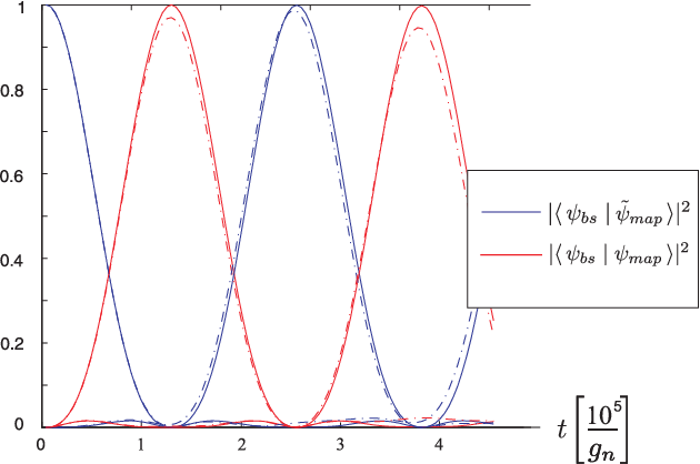
To illustrate that $H_{el}$, in the bosonic description, which we denote by $H_{bs}$, provides a good approximation to $H$ and allows to implement a good quantum interface, we consider a maximally entangled state $\sum_{k}\left|k\right>_{R}\left|k\right>_{c}$ of cavity and some reference system $R$ and then use the interface to map the state of the cavity to the nuclei. If a maximally entangled state of $R$ and nuclei is obtained, it shows that the interface is perfect for the whole subspace considered. The fidelity of the state $\mathbbm{1}_{R}\otimes U(t)\sum_{k=1}^{2}\left|k\right>_{R}\left|k\right>_{c}\left|0\right>_{n}$ with the maximally entangled state $\sum_{k}\left|k\right>_{R}\left|0\right>_{c}\left|k\right>_{n}$ fully quantifies the quality of the interface. In Fig. 5 we plot this fidelity for the evolutions $U(t)$ generated by the two Hamiltonians $H$ and $H_{el}$ of Eqs. (17) and (16) to show that a high-fidelity mapping is possible with the chosen parameters and that the simple Hamiltonian $H_{el}$ well describes the relevant dynamics. Since $U(\pi/g)aU(\pi/g)^{\dagger}=ib$ some care must be taken concerning the phases of the number state basis vectors in the nuclear spin mode ($\left|k\right>_{c}\mapsto(i)^{k}\left|k\right>_{n}$) and different phases at $t=3\pi/g$. For the numerical simulation, we chose the parameters as follows: the number of nuclei $N=10^{4}$, the hyperfine coupling constant $A=100\mu eV$, the laser and cavity Rabi frequency $\Omega_{c}=\Omega_{l}=6\mu eV$, the detuning of the trion $\omega_{X}-\omega_{l}=700\mu eV$, the microwave Rabi frequency $\Omega_{mw}=50\mu eV$ and the effective Zeeman splitting $\tilde{\omega}_{z}=50\mu eV$. This corresponds to $\sim 4$T using an electron g-factor of $0.48$ (external and Overhauser field are counter-aligned) and the corresponding hole Zeeman splitting $\omega_{mw}\sim 700\mu$eV. With these parameters, a value of $g\sim 5\cdot 10^{-5}\mu$eV is obtained, leading to times of $\sim 10$ microseconds for an interface operation.

Throughout the discussion we have neglected the internal nuclear dynamics and corrections to the bosonic description. Nuclear dynamics is caused by direct dipole-dipole interaction and electron-mediated interaction [7, 24, 25]. In [15] we consider these processes in detail and show that they are negligible: the coupling of the bosonic mode $b$ to bath modes $b_{k}$ is by a factor $10^{-2}$ smaller than the coupling $g$ in $H_{\mathrm{bs}}$ given by Eq. (18).
The bosonic description of the nuclear spin system can be introduced in a formally exact way [12]. However, to obtain the simple Jaynes-Cummings-like Hamiltonian Eq. (7) instead of Eq. (6) we have made several approximations. As discussed in more detail in Appendix B, these can lead to two types of errors, (i) an inhomogeneous broadening of $\omega_{2}$ and (ii) leakage from the mode $b$ due to inhomogeneity. High polarization reduces both effects. The broadening of $\omega_{2}$ can be further reduced by an accurate determination of the Overhauser shift $A^{z}$. Reduced Overhauser variance has already been seen experimentally [26, 27, 28]. Leakage is suppressed by the energy difference of excitations in the mode $b$ and the other modes not directly coupled to the electron [13] (cf. also the Appendix).

Finally, sufficiently small electron and cavity decoherence must be ensured. In particular, we assume the strong coupling limit of cavity-QED and neglect spontaneous emission for the whole duration of our protocol, which requires that $(\Omega_{l}/\Delta_{\pm})^{2}\gamma_{\mathrm{spont}}1/g\ll 1$, where $\gamma_{\mathrm{spont}}$ comprises spontaneous emission of the quantum dot into non-cavity modes. With the parameters chosen above this requires $\gamma_{\mathrm{spont}}\gg 1\mu$s^-1. Electron spin relaxation is sufficiently slow in QDs at large Zeeman splitting ($\gtrsim 1$ms) compared to our interaction. The effect of electron spin dephasing processes is suppressed by elimination of the electron: they lead to an inhomogeneous broadening of $g$ and $\omega_{i}$ which is small as long as the energy scale of the dephasing is small compared to the detuning $\tilde{\omega}_{z}$.

We have shown how to realize a quantum interface between the polarized nuclear spin ensemble in a singly charged quantum dot and a traveling optical field by engineering beam splitter and two-mode squeezer Hamiltonians coupling the collective nuclear spin excitation and the mode of the open cavity. This indicates how to optically measure and coherently manipulate the nuclear spin state and opens a path to include nuclear spin memories in quantum information and communication applications. Moreover, together with a photo detector for the output mode of the cavity, the quantum dot–cavity system provides a means to monitor nuclear spin dynamics on a microsecond time scale and would allow to precisely study the effect of internal nuclear spin dynamics and the corrections to the bosonic description used here.

References

- [1] H. J. Kimble, Nature 453, 1023 (2008).
- [2] A. Imamoğlu, D. D. Awschalom, G. Burkard, D. P. DiVincenzo, D. Loss, M. Sherwin, and A. Small, Phys. Rev. Lett. 83, 4204 (1999), eprint quant-ph/9904096, URL http://link.aps.org/abstract/PRL/v83/p4204.
- [3] W. Yao, R.-B. Liu, and L. J. Sham, Phys. Rev. Lett. 95, 030504 (2005), eprint cond-mat/0508441, URL http://link.aps.org/abstract/PRL/v95/e030504.
- [4] K. Hennessy, A. Badolato, M. Winger, D. Gerace, M. Atature, S. Gulde, S. Fält, E. L. Hu, and A. Imamoğlu, Nature 445, 896 (2007), eprint quant-ph/0610034, URL http://dx.doi.org/10.1038/nature05586.
- [5] R. Hanson and D. D. Awschalom, Nature 453, 1043 (2008).
- [6] J. M. Taylor, A. Imamoğlu, and M. D. Lukin, Phys. Rev. Lett. 91, 246802 (2003), eprint cond-mat/0308459.
- [7] J. Schliemann, A. Khaetskii, and D. Loss, J. Phys: Cond. Mat. 15, R1809 (2003), eprint cond-mat/0311159.
- [8] P. Maletinsky, Ph.D. thesis, ETH Zürich, http://e-collection.ethbib.ethz.ch/view/eth:30788 (2008).
- [9] A. S. Bracker, E. A. Stinaff, D. Gammon, M. E. Ware, J. G. Tischler, A. Shabaev, A. L. Efros, D. Park, D. Gershoni, V. L. Korenev, et al., Phys. Rev. Lett. 94, 047402 (2005), eprint cond-mat/0408466.
- [10] J. Skiba-Szymanska, A. V. Nikolaenko, M. N. Makhonin, I. Drouzas, M. S. Skolnick, A. B. Krysa, and A. I. Tartakovskii, Phys. Rev. B 77, 165338 (2008), eprint arXiv:0710.2837v1 [cond-mat.mes-hall], URL http://link.aps.org/abstract/PRB/v77/e165338.
- [11] A. Imamoğlu, E. Knill, L. Tian, and P. Zoller, Phys. Rev. Lett. 91, 017402 (2003), eprint cond-mat/0303575.
- [12] H. Christ, Ph.D. thesis, TU München (2008).
- [13] Z. Kurucz, M. W. Sørensen, J. M. Taylor, M. D. Lukin, and M. Fleischhauer, Phys. Rev. Lett. 103, 010502 (2009), eprint arXiv:0902.4566v1 [cond-mat.mes-hall], URL http://link.aps.org/doi/10.1103/PhysRevLett.103.010502.
- [14] E. Brion, L. Pedersen, and K. Mølmer (2006), eprint arXiv:quant-ph/0610056v1, URL http://arxiv.org/abs/quant-ph/0610056.
- [15] H. Schwager, J. I. Cirac, and G. Giedke, arXiv:0903.1727v1 (2009).
- [16] J. I. Cirac, P. Zoller, H. J. Kimble, and H. Mabuchi, Phys. Rev. Lett. 78, 3221 (1997).
- [17] M. Toishi, D. Englund, A. Faraon, and J. Vuckovic, Opt. Exp. 17, 14618 (2009).
- [18] S. L. Braunstein and H. J. Kimble, Phys. Rev. Lett. 80, 869 (1998).
- [19] C. W. Gardiner and P. Zoller, Quantum Noise (Springer Verlag, Berlin, 2000), 2nd ed.
- [20] G. Giedke, J. Eisert, J. I. Cirac, and M. B. Plenio, J. Quant. Inf. Comp. 3(3), 211 (2003), eprint quant-ph/0301038.
- [21] K. Hammerer, M. Wolf, E. Polzik, and J. Cirac, Phys. Rev. Lett. 94, 150503 (2005), eprint arXiv:quant-ph/0409109, URL http://link.aps.org/abstract/PRL/v94/e150503.
- [22] J. Fiurášek, Phys. Rev. A 66, 012304 (2002), eprint quant-ph/0202102.
- [23] K. Hammerer, E. Polzik, and J. Cirac, Phys. Rev. A 74, 064301 (2006), eprint quant-ph/0608133.
- [24] W. Yao, R.-B. Liu, and L. J. Sham, Phys. Rev. B 74, 195301 (2006), eprint cond-mat/0508441, URL http://link.aps.org/abstract/PRB/v74/e195301.
- [25] W. M. Witzel and S. Das Sarma, Phys. Rev. B 74, 035322 (2006), eprint cond-mat/0512323, URL http://link.aps.org/abstract/PRB/v74/e035322.
- [26] A. Greilich, A. Shabaev, D. R. Yakovlev, A. L. Efros, I. A. Yugova, D. Reuter, A. D. Wieck, and M. Bayer, Science 317, 1896 (2007), eprint http://www.sciencemag.org/cgi/reprint/317/5846/1896.pdf, URL http://www.sciencemag.org/cgi/content/abstract/317/5846/1896.
- [27] X. Xu, W. Yao, B. Sun, D. G. Steel, A. S. Bracker, D. Gammon, and L. J. Sham, Nature 459, 1105 (2009), URL http://www.nature.com/nature/journal/v459/n7250/full/nature08%120.html.
- [28] C. Latta, A. Högele, Y. Zhao, A. N. Vamivakas, P. Maletinsky, M. Kroner, J. Dreiser, I. Carusotto, A. Badolato, D. Schuh, et al., Nature Physics 5, 758 (2009), eprint arXiv:0904.4767, URL http://arxiv.org/abs/0904.4767.
- [29] T. Holstein and H. Primakoff, Phys. Rev. 58, 1098 (1940).
- [30] F. T. Arecchi, E. Courtens, R. Gilmore, and H. Thomas, Phys. Rev. A 6, 2211 (1972).
- [31] J. Fischer, M. Trif, W. A. Coish, and D. Loss (2009), eprint arXiv:0903.0527 [cond-mat].