The shape of disorder broadened Landau subbands in graphene
Abstract
Density of states (DOS) of graphene under a high uniform magnetic field and white-noise random potential is numerically calculated. The disorder broadened zero-energy Landau band has a Gaussian shape whose width is proportional to the random potential variance and the square root of magnetic field. Wegner-type calculation is used to justify the results.
pacs
81.05.Uw, 71.55.-i, 71.23.-kGraphene is a two-dimensional (2D) system that has attracted a lot of attentions in recent years[1, 2] because of the distinct and similar electron properties between graphene and conventional 2D electron gases such as the inversion layers of semiconductor heterostructures. Different from the usual 2D electrons in solids that obey Schrodinger equation, the governing equation of electrons in undoped graphene is the relativistic massless Dirac equation [3] due to the linear dispersion near the vicinity of the two nonequivalent corners and of the first Brillouin zone. Similar to the 2D Schrodinger electrons, 2D Dirac electron states in a perpendicular uniform magnetic field also form highly degenerated discrete Landau levels (LLs). Instead of equal spaced LLs for the Schrodinger electrons, the LLs of 2D Dirac electrons are unevenly distributed[4, 5] according to
| (1) |
where is the Fermi velocity, is electron charge and is the Planck constant. The existence of zero-energy Level for is a direct consequence of charge-hole symmetry. In the presence of disorders, LLs broaden into Landau subbands, gives raise to the quantum Hall effects[6]. The distribution of electron levels inside the Landau bands is a subject of fundamental interest because it is important to physics quantities sensitive to the density of states (DOS). For 2D Schrodinger electrons, the subject have been studied both theoretically and experimentally for a long time[7, 8, 9, 10, 11, 12, 13, 14, 15]. Based on self-consistent Born approximation (SCBA), the shape of DOS was argued to be the well-known semicircle form[7]. Later, Wegner predicted that the shape of the lowest LL in the strong-field limit and with white-noise random potential[8] is Gaussian-like. The supersymmetry method reaches the similar conclusions[10, 12]. However, the shape of disorder broadened Landau bands for the Dirac electrons is less well studied although it is important for the issues of diagonal and non-diagonal conductivity[16]. In this paper, we show that the shape of zero-energy Landau band is best described by Gaussian function. The broadening width of the band depends on both the magnetic field and disorder randomness. In the high magnetic field, it is proportional to the square-root of the field. At a fixed field, the broadening width is approximately linear in the square-root of disorder potential variance. Interestingly enough, these results are similar to the predictions of Wegner[8] on Schrodinger electrons. To demonstrate the importance of the shape of Landau subband in electron transport in high magnetic field, the magneto-conductivity is calculated.
The electrons of graphene in a perpendicular magnetic field can be modeled by a tight-binding Hamiltonian on a honeycomb lattice of two sites per unit cell,
| (2) |
where is the hopping energy between the nearest neighboring atoms. To mimic randomness on Dirac electrons, the on-site energy is assumed to be random with Gaussian white-noise distribution of zero mean and finite variance . measures randomness. The magnetic field is introduced by means of Perierls’ substitution in hopping parameter[17, 18] as , where .
In order to obtain numerically an accurate averaged DOS of the above Hamiltonian, the system size should be large enough so that the Lanczos recursive method[19] is used. The averaged DOS can be evaluated by , where is an infinitesimal positive number. The bar denotes the ensemble average. When disorder is present, the system does not have translational symmetry and all sites are no longer equivalent. Estimating the average by using the ”site-basis” is therefore inefficient. Inspired by the work of Triozon[20], we use the random phase state[21]. Thus we only need to consider several random phase states to get a good estimate of the average DOS. In this approach, a small artificial cut-off energy () is introduced to simulate the infinitesimal imaginary energy [22, 23]. This artificial parameter will lead to a small width of LLs in clean graphene.
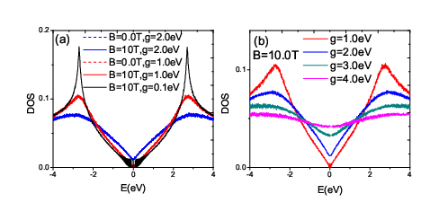
Both on-site energy randomness and the magnetic field can affect DOS. There are two important length scales. Disorder causes electron scattering, leading to an electron mean-free path . The magnetic field introduces a magnetic length . Electronic states in a Landau level (LL) can be viewed as cyclotron motions of an electron around orbits of radius centered at different location. Scattering can destroy and modify these cyclotron motions, leading to Landau subband broadening. Thus, one can expect different DOS at two limits, and . Fig. 1a is the DOS for . Indeed, our numerical results show that the DOSs at and strong disorder (in the sense of ) are almost the same as DOS at zero field and finite , showing no obvious magnetic field dependence of the Landau subbands in the limit. Fig. 1b shows DOS of different at a fixed field at which is still satisfied. The van Hove singularities is less singular as increases whereas the DOS near the Dirac point () increases with . These results agree with prior analytical results[24]. In the opposite limit (high magnetic field), the strength of random potential becomes relative weak such that Dirac electrons can complete their cyclotron motion before encountering scatters. For eV, we observed the oscillation of the DOS near the Dirac point as shown in Fig. 1(a), which reflects the appearance of LLs in high magnetic field. In what follows, we focus on the Landau subband broadening in high magnetic field.
In the limit of , DOS shows a very different behavior. Fig. 2a is the DOS of graphene without disorder () and in a uniform magnetic field (). like spectrum distributed according to Eq. (1) is observed. The seemingly non-zero width is due to the finite size effect and cut-off energy meV introduced in our numerical calculation. Furthermore, these finite-size broadened spectrum can be fitted well by Lorentizian distribution of 2meV width (from the cut-off energy). This artificial broadening may also be viewed to be a true broadening accounting the electron-phonon or electron-electron interactions in reality.
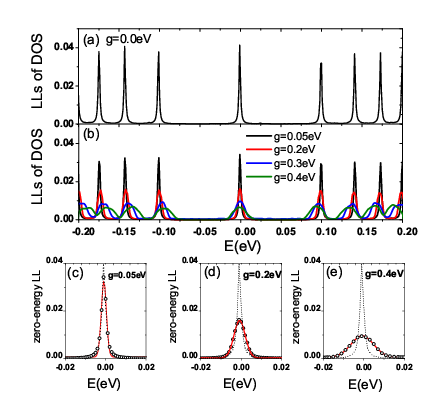
Fig. 2b is the DOS of Landau subbands at for various . The LLs degeneracy are lifted in the presence of disorder, LLs are broadened into Landau subbands. The broadening width () of zero-energy subband increases from meV to meV when changes from eV to eV. When the strength of the white-noise potential is very weak (eV), the broadening width of each Landau band increases a little. As shown in Fig. 2c (eV), the shape of the zero-energy Landau band is similar to the clean case and broadened by the disorder is as small as . In this case, the dominant factor on the subband shape is still the artificial cut-off energy. However, the broadening width of zero-energy Landau subband becomes large for eV when the disorder dominate the band broadening and the artificial cut-off energy is irrelevant. Numerical results show that the broadening shape of zero-energy Landau subband changes also from the Lorentizian shape to the Gaussian one. Figs. 2d-2e show that DOS can be fitted well by the Gaussian function, suggesting DOS of zero-energy Landau subband is Gaussian in the presence of a white noise potential[25, 26]. This finding is very similar to the Gaussian-like shape for the lowest LL for 2D Schrodinger electrons[8, 9, 10, 11, 12, 13, 14, 15].
As shown in Fig. 2b, Landau subbands are distorted and shifted toward zero energy direction in the presence of white-noise disorder[27] except the zero-energy subband because disorder does not destroy the electron-hole symmetry. This disorder effect can be seen clearly from the noticeable move of the DOS peak positions of bands. This shift of DOS peaks can be qualitatively explained within the Self-consistent non-crossing approximation (SCNCA)[28]. According to SCNCA, DOS peak positions should move toward zero energy in the presence of white-noise disorder due to the finite real part of the self energies, and the shift increases with . However, SCNCA fails to account for the shape of broadened bands.
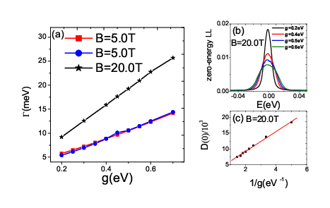
Fig. 3a shows the dependence of subband width for the zero-energy subband () for and . As expected, of zero-energy Landau subband increases with . The same dependence is obtained for the first () Landau subband (squares). The data shows approximately a linear dependence in . The slop depends on the magnetic field. However, the width does not depends on the band index as suggested by the complete overlap of for (circles) and for (squares) at . Fig. 3b shows the DOS of zero-energy subband at for various disorder . The peak decreases with , and is proportional to the inverse of as shown by the good linear fit in Fig. 3c. This is because the total number of states in each Landau subband is a constant which is the total number of flux quanta in the system. Since is proportional to , to keep the area defined by the DOS curve and E-axis to a constant, the peak must be roughly follow dependence. More interestingly, the shape of zero-energy subband remains symmetric due to electron-hole symmetry, and may follow a true Gaussian distribution.
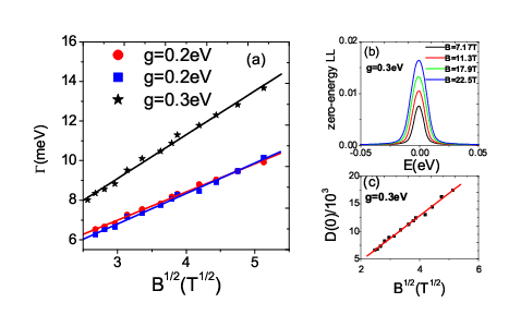
Fig. 4 is the magnetic field dependence of DOS at a fixed . Fig. 4a shows square-root field dependence of for both band and band. The good overlap of for the two subbands at eV suggests that, similar to the dependence, curves are universal (independent on band indices). Just like DOS- dependence, Fig. 4b shows how DOS of zero-energy band change with magnetic field. It is clear that is proportional to square-root of as shown in Fig. 4c. This is because the total number of states in one Landau subband is proportional to , thus the product of the band peak () and bandwidth should be proportional to .
In order to understand our numerical findings quantitatively, we generalize the approach of Wegner[8] for Schrodinger electrons to the Dirac electrons to obtain an analytic expression of DOS for the zero-energy band since it is only valid for small . In the high magnetic field regime, the Green’s function of unperturbed system for the zero-energy band is
| (3) |
with
where and are the complex variables. is the degeneracy per area in each LL for the clean graphene. If the intervalley scattering between and is ignored, the Green’s function of the zero-energy LL has only one non-zero term, which simplifies the problem a lot. In this case, the shape of zero-energy LL can be directly mapped to the problem of conventional 2DEG for the lowest LL[8]. Therefore, the shape of the zero-energy band has a Gaussian-like form:
| (7) |
This Gaussian-like form is little bit flater than the true Gaussian distribution. Although our numerical date can also fit this Gaussian-like form, but they fit the Gaussian function better. This may be due to the fact that intervalley scattering is neglected in our derivation of the Gaussian-like form while our numerical calculation include all effects from both disorders and magnetic field.
The shape of Landau bands is important to many physical quantities. As an example, we would like to evaluate the magneto-conductivity of a band whose DOS is a Gaussian function. In the Drude-Boltzemann approximation, the Kubo formula yields the diagonal magneto-conductivity for the Fermi energy at the Dirac point[30]:
| (8) |
where and is cyclotron frequency. Although Eq. (4) works well only in the high magnetic field (). Noted that is independent on as , thus magneto-conductivity does not depend on the magnetic field, and is only disorder dependent. This behavior reflects that should tend to saturate in high magnetic field, which is consistent with the experimental observations of Ref.[31].
In conclusion, the shape of disorder broadened zero-energy Landau band can be described well by a Gaussian function. For white-noise random potential, band width is proportional to both the square-root of magnetic field and variance of random potential. The perturbation theory is used to justify the conclusions. The importance of the shape of Landau bands is demonstrated by the magneto-conductivity. The results can shield some lights on the properties of graphene in magnetic field.
This work is partially supported by the National Natural Science Foundation of China (Grant nos. 10574119). The research is also supported by National Key Basic Research Program under Grant No. 2006CB922000. X. R. Wang is supported by UGC/RGC grants. Jie Chen would like to acknowledge the funding support from the National Institute of Nanotechnology and from the Discovery program of Natural Sciences and Engineering Research Council of Canada under Grant No. 245680.
References
- [1] K. S. Novoselov, et al., Science 306, 666 (2004).
- [2] K. S. Novoselov, et al., Nature 438, 197 (2005).
- [3] A. K. Geim and K. S. Novoselov, Nature Mater. 6, 183 (2007).
- [4] Zheng Y. and Ando T. , Phys. Rev. B 65, 245402(2002).
- [5] Guohong Li and Eva Y. Andrei, Nature Phys. 3, 623(2007).
- [6] The Quantum Hall Effect, edited by Richard E. Prange and Steven M. Grivin, Springer-Verlag(1987).
- [7] T. Ando, Rev. Mod. Phys. 54, 437(1983).
- [8] Franz Wegner, Z. Phys. B 51, 279(1983).
- [9] Ian Affleck, J. Phys. C 17, 2323(1984).
- [10] E. Br¨¦zin, David J. Gross and C. Itzykson, Nuclear Physics B 235, 24(1984).
- [11] Rolf R. Gerhardts, Z. Phys. B 21, 275(1975): Rolf R. Gerhardts, Z. Phys. B 21, 285(1975).
- [12] Supersymmetry in Disorder and Chaos, K.B. Efetov, Cambridge University Press(1997).
- [13] E. Gronik, et al., Phys. Rev. Lett. 54, 1820(1985).
- [14] T. P. Smith, et al., Phys. Rev. B. 32, 2696(1985).
- [15] E Stahl, et al., J. Phys. C. 18, L783(1985).
- [16] O Viehweger, et al., J. Phys. Condens. Matter. 3, 1675(1991).
- [17] X.R. Wang, Phys. Rev. B 51, 9310 (1995); 53, 12035 (1996).
- [18] A. L. C. Pereira and P. A. Schulz, Phys. Rev. B. 78, 125402(2008); A. L. C. Pereira and P. A. Schulz, Phys. Rev. B 77, 075416 (2008); R. Saito, G. Dresselhaus and M. S. Dresselhaus, Physical Properies of Carbon Nanotubes ,Imperial College Press, London(1998).
- [19] Periodic boundary condition are used. Typical supercell size contains millions of carbon atoms.
- [20] F. Triozon, et al.. Phys. Rev. B 69, 121410, (2004).
- [21] The random phase states are placed in the middle of the system and extend over a (possibly large) number of orbitals, Ni: , where is a random number in the interval .
- [22] The relationship between and the system size () has been shown in Ref.[23]. In the region , decreases very slowly when gets larger. If one wants to reduce to , a much large system size is needed.
- [23] Shangduan Wu, et al., Phys. Rev. B 77, 195411(2008).
- [24] Balazs Dora, et al., Phys. Rev. B 77, 115422(2008).
- [25] We also find other arbitrary uncorrelated short range impurity potential(such as Anderson disorder) can result in the Gaussian shape of broadening LLs, which is the same with the results in 2DEG as well[6].
- [26] B. Kramer, et al., Z. Phys. B 56, 297(1984).
- [27] N. M. R. Peres, et al., Phys. Rev. B 73, 125411(2006).
- [28] Balazs Dora, Fizika Nizkikh Temperatur, 34, 1020(2008).
- [29] Nguyen Hong Shon and T. Ando, JPSP 67, 2421(1998).
- [30] W. Zhu, et al., Chin. Phys. Soc. 57, 3775(2007).
- [31] Sungjae Cho and Michael S. Fuhrer, Phys. Rev. B 77, 081402(2008).