Binding bigraphs
as symmetric monoidal closed theories

We should start our overview with the definition of smc categories: these are symmetric monoidal categories, i.e., categories with a tensor product $\otimes$ on objects and morphisms, symmetric in the sense that $A\otimes B\cong B\otimes A$, such that $(-\otimes A)$ has a right adjoint $(A\multimap-)$, for each $A$. We do not give further details, since we are interested in describing the free such category, which happens to be easier. Knowing that there is a category $\mathsf{SMCCat}$ of smc categories and strictly structure-preserving functors should be enough to grasp the following.

As sketched in the introduction, a signature $\Sigma$ is given by a set $X$ of sorts, equipped with a graph whose vertices are imll formulae over $X$, as defined by the grammar:

We think of each edge $A\to B$ of the graph as specifying an operation of type $A\to B$. A morphism of signatures $(X,\Sigma)\to(Y,\Sigma^{\prime})$ is a function $X\rTo^{f}Y$, equipped with a morphism of graphs, whose vertex component is “$\mathcal{F}(f)$”, i.e., it sends any formula $A(x_{1},\ldots,x_{n})$ to $A(f(x_{1}),\ldots,f(x_{n}))$. This defines a category $\mathsf{SMCSig}$ of signatures.

There is then a forgetful functor $\mathsf{SMCCat}\rTo^{U}\mathsf{SMCSig}$ sending each smc category $\mathcal{C}$ to the graph with

vertices:

formulae in $\mathcal{F}(\ob(\mathcal{C}))$, and

edges $A\to B$:

morphisms $\llbracket A\rrbracket\to\llbracket B\rrbracket$ in $\mathcal{C}$, where $\llbracket A\rrbracket$ is defined inductively to send each syntactic connective to the corresponding function on $\ob(\mathcal{C})$.

Trimble [7] constructs an smc category $S(\Sigma)$ from any signature $\Sigma$, which extends to a functor $\mathsf{SMCSig}\rTo^{S}\mathsf{SMCCat}$, left adjoint to $U$: for any smc category $\mathcal{C}$ and natural transformation $\Sigma\rTo^{f}U(\mathcal{C})$, there is a unique smc functor $S(X)\rTo^{f^{*}}\mathcal{C}$ such that $f$ decomposes as {diagram}

How does $S(\Sigma)$ look like? Its objects are imll formulae in $\mathcal{F}(X)$ and morphisms are kind of proof-nets with some cells representing operations. A morphism from $A$ to $B$ in $S(\Sigma)$ thus consists of

• •

  a finite set $C=\{c,\ldots\}$ of cells labelled by operations $\alpha_{c}\to\beta_{c}$ in $\Sigma$,

• •

  and wires connecting the ports together.

For example in the $\pi$-calculus, the operations $\mathit{get}$ and $\mathit{send}$ correspond to cells:

We always use the flat edge (or base) of the polygon to denote the domain. The orientation of a port corresponds to its sign, see below.

A port is a leaf occurrence (atomic or $I$) in $A$, $B$, or in some $\alpha_{c}$, $\beta_{c}$. Equivalently, a port is a leaf occurrence in the formula

(or $A\multimap B$ when $C$ is empty). In a formula, a port is positive when it lies to the left of an even number of $\multimap$’s, and negative otherwise²² 2 The sign of a port in $A$ is directly apparent viewing $A$ is a classical LL formula, see the next paragraph.. The sign of a port in a morphism is its sign in the formula (2).

Wires are oriented, with sources the negative ports of the morphism, and targets in its positive ports. For each sort $x\in X$, the wires must induce a bijection between ports labelled $x$ (which we call $x$ ports). A negative $I$ port can be wired to any positive port.

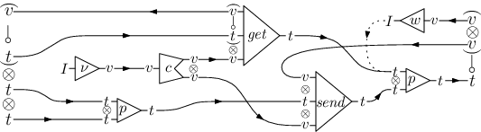
An example of morphism is presented in Fig. 1, where $\Sigma$ has sorts $\{t,v\}$ and operations $\mathit{get}$, $\mathit{send}$, $v\rTo^{c}v\otimes v$, $I\rTo^{\nu}v$ and $t\otimes t\rTo^{p}t$.

That gives the construction for signatures. We now extend it to smc theories: define a theory $\mathcal{T}$ to be given by a signature $\Sigma$, together with a set $E_{A,B}$ of equations between morphisms in $S(\Sigma)(A,B)$, for each imll formulae $A,B$. The free smc category $S(\mathcal{T})$ generated by such a theory is defined in our note [18] to be the quotient of $S(\Sigma)$ by the equations. Constructing $S(\mathcal{T})$ graphically is more direct than could have been feared: we first define the binary predicate $f_{1}\sim f_{2}$ relating two morphisms $C\pile{\rTo^{f_{1},f_{2}}\\ \rTo}D$ in $S(\Sigma)$ as soon as each $f_{i}$ decomposes as {diagram} with a common $f$, with $(g_{1},g_{2})\in E_{A,B}$, and where $\ulcorner g\urcorner$ is the currying of $g$. Then, we take the smallest generated equivalence relation, prove it stable under composition, and quotient $S(\Sigma)$ accordingly, which yields the free smc category $S(\mathcal{T})$ generated by the theory $\mathcal{T}=(\Sigma,E)$.

We fix such a bigraphical signature $\mathcal{K}$ for the rest of the paper. This signature can be translated into a smc signature $\Sigma_{\mathcal{K}}$ over two sorts $\{t,v\}$, standing for terms and variables (or names). It consists of the following structural operations, accounting for the built-in structure of bigraphs:

plus, for all controls $k$, a logical operation

where $x=I$ if $k$ is atomic and $x=t$ otherwise.

We call $\mathcal{T}_{\mathcal{K}}$ the theory consisting of the operations in $\Sigma_{\mathcal{K}}$, with the equations making

• •

  $(t,\mid,\mathbf{0})$ into a commutative monoid object,

• •

  $(v,c,w)$ into a cocommutative comonoid object ($c$ is coassociative, cocommutative, and $w$ is its unit), and

• •

  $\nu$ and $w$ annihilate each other, as in

  

  $\cdot$

We now proceed to describe the category $\mathbf{Bbg}(\mathcal{K})$ of abstract binding bigraphs over $\mathcal{K}$, which we relate in Section 4 to the free model $S(\mathcal{T}_{\mathcal{K}})$ of $\mathcal{T}_{\mathcal{K}}$.

We assume an infinite and totally ordered set $\mathcal{X}$ of names.

A name $x$ is said global if $\mathit{loc}(x)=\bot$ and local or located at $i$ when $\mathit{loc}(x)=i\in n$.

Bigraphical interfaces are the objects of the category $\mathbf{Bbg}(\mathcal{K})$. We define a function $\mathsf{T}$ from these objects to imll formulas, i.e., objects of $S(\mathcal{T}_{\mathcal{K}})$, by:

where $n_{g}=|\mathit{loc}^{-1}(\bot)|$ and for all $i\in n$, $n_{i}=|\mathit{loc}^{-1}(i)|$. The ordering on $\mathcal{X}$ induces a bijection between $X$ and $v$ leaves in the formula.

In [22], Milner presents a slight generalisation of binding bigraphs, where names have multiple locality. Some interfaces cannot be simply translated into imll formulas as before, e.g., if $x$ is located in $0$ and $1$ and $y$ in $1$ and $2$, this dependency cannot be expressed directly in an imll formula.

Let $n$ and $m$ be two finite ordinals.

The ordinals $n$ and $m$ index respectively the sites and roots. A node is said barren if it has no preimage under the parent map (atomic nodes are thus barren).

The relation $\prec$ over sites, roots and nodes defined by:

is a (strict) partial order. The maximal elements of $\prec$ are the roots; the minimal elements are the barren nodes (including atomic nodes) and the sites.

Let $X$ and $Y$ be two finite sets of names.

This binding rule is not mentionned in the original paper [1] about bigraphs whereas it is mandatory for the scoping discipline to be stable under composition (it is added in [22]). Alternatively, we can only require $\mathit{link}(p)$ to not be a global name of $Y$; the scope rule (defined below) handles the case of local names of $Y$.

We define the binders of our link graph to be the local names of $Y$ (located at a root) and the binding ports (located at a node) $P_{B}$. Two distinct points (i.e.,  two elements of $P+X$) $x$ and $y$ are peers when $\mathit{link}(x)=\mathit{link}(y)$. An edge is idle when it has no preimage under the link map.

Let $U=(n,X,\mathit{loc})$ and $W=(m,Y,\mathit{loc}^{\prime})$ be two bigraphical interfaces.

The binding rule ensures that no binding port $p$ is peer of a name in $Y$, hence $\mathit{link}(p)$ has to be an edge. Moreover, by acyclicity of $prnt$, no two binding ports may be peers, hence edges are linked to at most one binding port. The set of edges may thus be decomposed into a set of free edges $E_{F}$ (without binding port) and a set of bound edges $E_{B}$ in one-to-one correspondence with $P_{B}$ by the link map: $E=E_{F}\uplus E_{B}\cong E_{F}+P_{B}$.

Finally, two bigraphs are lean-support equivalent when after discarding their idle edges, there is an isomorphism between their sets of nodes and edges preserving the structure.

The composition of two bigraphs {diagram} is defined by taking the coproduct of their nodes, edges and control maps and the composition of parent and link maps (modulo some bijections on sets), forgetting the roots/sites from $U_{2}$. Acyclicity of the parent map, and the binding and scope rules are preserved by composition.

First, since $(t,|,\mathbf{0})$ has a commutative monoid object structure, the representation of Section 2.3 applies: we just have to define a function from negative $t$ ports to positive ones. Now, for any set $X$ labeled in formulae, denote by $X^{+}_{t}$ its set of positive $t$ ports, and similarly for $X^{+,-}_{t,v,I}$. Now, considering each cell $c$ to be labelled by the formula $\alpha_{c}\multimap\beta_{c}$, we have:

• •

  $C^{+}_{t}\cong V$, because each type of cell $K_{k}$ has one positive $t$ port,

• •

  $C^{-}_{t}\cong V_{\mathit{na}}\hookrightarrow V$, where $V_{\mathit{na}}$ is the set of non-atomic nodes, because there is one negative $t$ port for each non-atomic cell,

• •

  $\mathsf{T}(U)^{+}_{t}\cong n$, because for each $i\in n$ there is a positive $t$ port in $\mathsf{T}(U)$,

• •

  similarly, $\mathsf{T}(W)^{+}_{t}\cong m$, and finally

• •

  $\mathsf{T}(W)^{-}_{t}\cong\mathsf{T}(U)^{+}_{t}\cong\emptyset$.

Our morphism $\mathsf{T}(G)$ is thus defined on the sort $t$ by the function $f_{t}$: {diagram}

The function $f_{v}$ for $v$ requires more work, and involves defining the structural support $C^{\prime}$. Recall that the data is the function $\mathit{link}:P\uplus X\to E\uplus Y$.

We start with an informal description of $f_{v}$ based on Fig. 5, in which bold arrows come from binders. First, we deal with points sent to edges. There are two kinds of edges.

First, we understand each free edge $e$ as the creation of a fresh name, and each free point $p$ in $P_{F}\uplus X$ sent to $e$ as an occurrence of this free name. Accordingly, $e$ is replaced by its $\nu$ cell in $C$, and each $p$ becomes a $v$ port in $\mathsf{T}(U)^{-}+C^{-}$. We hence link the $v$ port of the $\nu$ cell to each corresponding $p$, through a tree of $c$ and $w$ cells, as depicted in the bottom row.

Second, we understand each bound edge $e$ as an indirection to its binding port $p_{0}\in P_{B}$, itself understood as a bound name. We further understand each free peer $p\in P_{F}\uplus X$ of $p_{0}$ as an occurrence of the bound name. Accordingly, we completely forget about $e$, $p_{0}$ becomes a $v$ port in $C^{+}$, and each $p$ becomes a $v$ port in $C^{-}+\mathsf{T}(U)^{-}$, hence we link $p_{0}$ to each corresponding $p$, again through a tree of $c$ and $w$ cells.

Finally, points $p$ not sent to an edge are sent to some name $y\in Y$. But each such $p$ becomes a $v$ port in $\mathsf{T}(U)^{-}+C^{-}$ and each such $y$ becomes a $v$ port in $\mathsf{T}(W)^{-}$, hence we link $y$ to each $p$, again using $c$ and $w$ cells. This determines the structural support $C^{\prime}$, as well as $f_{v}$. Finally, for the $I$ part $f_{I}$, each negative $I$ port arises from a structural $w$ cell. But in the above each cell is generated by one $v$ port (the fresh name or the binder). In the former case, we may safely link our $I$ port to any valid $t$ port. In the latter, the binder occurs to the left of a $\multimap$, whose right-hand side is a $t$ port, to which we safely link our $I$ port.

More formally, observe from our translation of signatures and interfaces, plus the logical support $C$ defined above, that:

• •

  each free edge in $E_{F}$ corresponds to one $\nu$ cell, hence to one port in $C^{+}_{v}$,

• •

  each binding port in $P_{B}$ corresponds to one negative occurrence of $v$ in the domain of some cell in $C$, hence to one port in $C^{+}_{v}$,

• •

  each local name in $Y$ corresponds one port in $\mathsf{T}(W)^{-}_{v}$.

Thus, we have an isomorphism $E_{F}+P_{B}+Y\cong C^{+}_{v}+\mathsf{T}(W)^{-}_{v}$. Similarly, free points in $P_{F}+X$ correspond to ports in $C^{-}_{v}+\mathsf{T}(U)^{-}_{v}$, i.e., $P_{F}+X\cong C^{-}_{v}+\mathsf{T}(U)^{-}_{v}$.

We may thus define a first function $\mathit{link}^{\prime}$ by:

We then encode this function by a forest of $c$ and $w$ cells $C^{\prime}$ (as pictured in Fig. 6), to obtain a function $C^{+}_{v}+C^{\prime+}_{v}+\mathsf{T}(W)^{-}_{v}\rTo^{f_{v}}C^{-}_{v}+C^{\prime-}_{v}+\mathsf{T}(U)^{-}_{v}$, which qualifies as the $v$ part of our morphism.

The rest follows similarly.

This defines a function from bigraphs to candidate morphisms (respecting domain and codomain). We now show that it extends to a functor.

First, we prove that the image of a bigraph is correct, i.e., is a proper morphism.

The following seems known [25]:

One sees at once that $\mathsf{T}$ is not full. For example, the morphism in Fig. 7 has no preimage – any such preimage would violate the scope rule for bigraphs.

This example reflects that it is not necessary to distinguish global and local variables in a bigraph with only one site. Nevertheless, the notion of scope is preserved by $\mathsf{T}$ because closed morphisms can actually be translated into bigraphs. In $\mathbf{Bbg}(\mathcal{K})$, define the interfaces $I=(0,\emptyset,\widehat{\emptyset})$ and $t=(1,\emptyset,\widehat{\emptyset})$.

All in all, we have

It is however not full and far from surjective on objects.

References

- [1] Jensen, O.H., Milner, R.: Bigraphs and mobile processes (revised). Technical Report TR580, University of Cambridge (2004)
- [2] Girard, J.Y.: Linear logic. Theoretical Computer Science 50 (1987) 1–102
- [3] Damgaard, T.C., Glenstrup, A.J., Birkedal, L., Milner, R.: An inductive characterization of matching in binding bigraphs. To appear (2008)
- [4] Rathke, J., Sobocinski, P.: Deconstructing behavioural theories of mobility. In: Fifth IFIP International Conference On Theoretical Computer Science - TCS ’08, Springer (2008)
- [5] Milner, R., Parrow, J., Walker, D.: A calculus of mobile processes. Information and Computation 100(1) (1992) 1–40
- [6] Cardelli, L., Gordon, A.: Mobile ambients. In Nivat, M., ed.: Foundations of Software Science and Computational Structures. Volume 1378 of Lecture Notes in Computer Science., Springer (1998) 140–155
- [7] Trimble, T.: Linear logic, bimodules, and full coherence for autonomous categories. PhD thesis, Rutgers University (1994)
- [8] Danos, V., Regnier, L.: The structure of multiplicatives. Archive for Mathematical Logic 28 (1989) 181–203
- [9] Debois, S.: Sortings & bigraphs. PhD thesis, IT University of Copenhagen (2008)
- [10] Pfenning, F., Elliott, C.: Higher-order abstract syntax. In: ACM SIGPLAN ’88 Symposium on Language Design and Implementation, ACM (1988) 199–208
- [11] Gabbay, M.J., Pitts, A.M.: A new approach to abstract syntax involving binders. In: 14th Annual Symposium on Logic in Computer Science, IEEE Computer Society Press, Washington (1999) 214–224
- [12] Hofmann, M.: Semantical analysis of higher-order abstract syntax. In: LICS ’99: Proc. 14th Annual IEEE Symposium on Logic in Computer Science, IEEE Computer Society (1999)
- [13] Sassone, V., Sobociński, P.: Deriving bisimulation congruences using 2-categories. Nordic Journal of Computing 10(2) (2003) 163–183
- [14] Bruni, R., Montanari, U.: Cartesian closed double categories, their lambda-notation, and the pi-calculus. In: LICS ’99: Proc. 14th Annual IEEE Symposium on Logic in Computer Science, IEEE Computer Society (1999) 246
- [15] Tan, A.: Full Completeness for Models of Linear Logic. PhD thesis, University of Cambridge (1997)
- [16] Hughes, D.J.D.: Simple free star-autonomous categories and full coherence. ArXiv Mathematics e-prints, math/0506521 (June 2005)
- [17] Lamarche, F., Strassburger, L.: From proof nets to the free *-autonomous category. Logical Methods in Computer Science 2(4) (2006)
- [18] Garner, R.H.G., Hirschowitz, T., Pardon, A.: Graphical presentations of symmetric monoidal closed theories. CoRR abs/0810.4420 (2008)
- [19] Barber, A., Gardner, P., Hasegawa, M., Plotkin, G.: From action calculi to linear logic. In: Annual Conference of the European Association for Computer Science Logic (CSL’97), Aarhus, August 1997, Selected Papers. Volume 1414 of Lecture Notes in Computer Science., Springer (1998) 78–97
- [20] Sassone, V., Sobociński, P.: Reactive systems over cospans. In: Logic in Computer Science, LiCS ’05, IEEE Press (2005) 311–320
- [21] Damgaard, T., Birkedal, L.: Axiomatizing binding bigraphs. Nordic Journal of Computing 13(1–2) (2006) 58–77
- [22] Milner, R.: Bigraphs whose names have multiple locality. Technical Report TR603, University of Cambridge (2004)
- [23] Grohmann, D., Miculan, M.: Directed bigraphs. Electr. Notes Theor. Comput. Sci. 173 (2007) 121–137
- [24] Hildebrandt, T.: Polarized and higher-order bigraphs from geometry of interaction. Talk at the Choco seminar, see http://choco.pps.jussieu.fr/events, Lyon (June 2008)
- [25] Soloviev, S.: Connectedness and acyclicity in IMLL proof nets (June 2008) Message to the TYPES forum.
Appendix 0.A Proof of Lemma 1
Consider a switching of .
Given a site or a node , we denote by the negative port corresponding to it in the switching. If is a root, then denotes the positive port of its image.
Free ports of a node (resp. local names of a site ) have their image (a positive port) connected to (resp. ) as shown in Fig. 8. Moreover, either one negative port (corresponding to a binding port) or the positive port of the cell is connected to by the switched formula.
We now prove by induction that all binding ports (located at a node or a root ) have their image connected to . Let be a binding port, and its image by (a negative port).
If has no peers (this is necessarily the case if is a barren node), then is connected to a cell whose port is connected to .
If has peers, then is connected, in the morphism, to their translations through a tree of cells. But this tree is heavily switched and only connects to one positive port (whose preimage is) located, thanks to the scope rule, to a site or a node .
By induction is connected to and is connected to through the (unswitched) parent map. Indeed, the parent map connects the ports of cells between and , and these cells have their ports connected thanks to the induction hypothesis. The port and are thus connected.
Finally, we remark that:
- •
roots are connected to each other in the codomain’s formula (by their or ports, see Fig. 8),
global variables of the domain are connected to a site (by the domain’s formula, see Fig. 8) and
remaining negative ports (global variable of the codomain and cells) are connected to the other positive ports by a switched tree of cells or a cell.
We conclude that all ports of our switching are connected.
Appendix 0.B Proof of Lemma 4
Consider any . We have and , which justifies our “induces” above. We now define such that .
Let the set of nodes be the set of logical cells in ; the control map sends each cell to .
The set of edges is the coproduct of binding ports in the support of and of cells (where a port is binding when it occurs to the left of a , e.g., a cell of type has two binding ports).
The parent map is exactly the restriction of to ports. The link map is obtained from the restriction of to ports as follows. From any port , following the tree of contractions towards its root leads to a maximal positive port in the support, which may be either a port from a cell, or a binding port of a logical cell. In each case, there is a corresponding edge . Our link map sends each port to . Since in each tree there is only one root, the binding rule is respected.
We then prove that is correct. Suppose that the parent map contains a cycle, then any switching where, for all cells of the cycle, the two ports are connected contains this cycle. Suppose that the scope rule is not satisfied for a binder and one of its peers . Then, in , is the root of a contraction tree with as a leaf: among the switchings connecting them, choose again one that connects both ports of each logical cell: every logical cell then has a path to the root (the port in the codomain), which forms a cycle involving , , and , hence contradicting correctness of . The binding rule is automatically satisfied because the codomain has no name. An atomic node has no antecedent in the parent map because the corresponding cell in has no positive port.