The hadronization of partons
Abstract
We review the description of inclusive single unpolarized light hadron production using fragmentation functions in the framework of the factorization theorem. We summarize the factorization of quantities into perturbatively calculable quantities and these universal fragmentation functions, and then discuss some improvements beyond the standard fixed order approach. We discuss the extraction of fragmentation functions for light charged (, and ) and neutral ( and ) hadrons using these theoretical tools through global fits to experimental data from reactions at various colliders, in particular from accurate reactions at LEP, and the subsequent successful predictions of other experimental data, such as data gathered at HERA, the Tevatron and RHIC from these fitted fragmentation functions as allowed by factorization universality. These global fits also impose competitive constraints on . Emphasis is placed on the need for accurate data from and reactions in which the hadron species is identified in order to constrain the separate fragmentation functions of each quark flavour and hadron species.
pacs
12.38.Cy,12.39.St,13.66.Bc,13.87.FhI Introduction
Fragmentation functions (FFs) constitute one of the most important free inputs required for a comprehensive description of most collider processes to which perturbative QCD is applicable, being a necessary ingredient in any sufficiently complete calculation of processes involving detected hadrons in the final state. They quantify the hadronization of quarks and gluons which must eventually occur in every process in which hadrons are produced. While parton distribution functions (PDFs), another of the important free inputs, are relevant for collisions involving at least one hadron, most importantly at present for collisions at the LHC, FFs are relevant in principle for all collisions, even those without any initial state hadrons such as electron-positron collisions at the future ILC. Furthermore, while knowledge and application of PDFs is limited to the types of hadrons that can be practically used in the initial state, being almost exclusively nucleons, FFs can be constrained by, and/or used for the predictions of, measurements of the inclusive productions of neutral and charged hadron species ranging from the almost massless to the very heavy. Such a large range of processes provides a large range of information on hadronization, and hence provides an important contribution to our understanding of non perturbative physics in general, and allows for a particularly incontrovertible phenomenological determination of the applicability and limitations of the various approximations used in the context of QCD factorization. Such data are also sufficiently accurate to allow for competitive extractions of , the strong coupling constant of QCD evolved for convenience to the -pole mass and the remaining of the most important free inputs, which improves the accuracy of perturbative QCD calculations in general and imposes constraints on new physics. We note here that while other inputs such as higher twist, multi-hadron FFs, fracture functions, and so on become important in certain kinematic limits, FFs are always necessary for a complete description of inclusive hadron production.
In this article, we review the progress in understanding the hadronization of partons, embodied in FFs, and their application to inclusive hadron production. The concept of fragmentation was first introduced by Feynman and Field in 1977 [1] to explain the limited transverse momenta and energy fraction scaling of hadrons in jets produced in collisions, as well as the presence of a few high transverse momentum () GeV hadrons in hadron-hadron collisions. In the latter case, the collision of a pointlike constituent particle of one hadron with that of another produces a pair of particles whose directions of motion are opposite to one another but at any angle to the parent particles, including large angles. These elementary particles must eventually hadronize to produce the high hadrons. Intuitively, any inclusive single hadron production processes may be predicted by first calculating the equivalent partonic process (i.e. replacing the produced hadron by a parton and the inclusive sum over hadron final states by partonic ones), then allowing the produced parton to hadronize. This parton model is made more precise by the factorization theorem.
Our discussion will be limited to inclusive single unpolarized hadron production, being better understood than its polarized counterpart. Final state partons will on average hadronize to hadrons of all species that are not kinematically forbidden by the particular reaction, but, of all the charged hadrons, partons will mostly hadronize to the 3 lightest ones, being , and , so their FFs are the most phenomenologically well constrained. (For a concise summary of the properties of some known mesons and baryons, see Ref. [2].) The species of neutral meson and neutral baryon most likely to be produced in the hadronization process are , and respectively, but their FFs are accurately approximated by the FFs for and due to SU(2) (nuclear) isospin symmetry between the and quark flavours. The next lightest species of meson and baryon is and respectively, whose FFs have therefore also been greatly studied. ( is not usually observed in experiment because it takes a long time to decay into charged particles.) Together with , , , , , , , and mesons, whose FFs are unfortunately either unknown or rather poorly known at present, the particles mentioned in this paragraph complete the list of known hadrons which have a mass less than or equal to the mass and which are the most copiously produced in hadron production, and thus measurements of their production lead to a rather comprehensive picture of the hadronic final state. In this review we shall focus on the productions of these particles only, with the exceptions of the productions of those mesons just listed.
Much of the techniques for global fitting of PDFs can be carried over to global fitting of FFs, for example the treatment of systematic errors on the experimental data and the propagation of experimental errors to the FFs, as well as the techniques used for the minimization of chi-squared. On the theoretical side, much of the formalism of both the fixed order (FO) calculations and its improvement via e.g. large resummation and incorporation of heavy quarks and their masses, is also very similar.
To date, the subject of fragmentation has been important in various areas of phenomenology [3], and we give an incomplete list of examples: Phenomenological constraints on the nucleon PDFs for polarized quarks and antiquarks separately, which are important for the determination of the source of nucleon spin, can be obtained from measurements of semi-inclusive DIS with polarized initial state particles for the inclusive production of single unpolarized light charged hadrons using knowledge of the FFs for these particles [4]. Valence quark PDFs can be similarly extracted, but from data for which the initial state particles are unpolarized [5]. In both cases, the differences between FFs for positively and negatively charged particles, are required, which are relatively poorly constrained by data from e.g. reactions, and not by accurate reaction data. Polarized reaction data from e.g. RHIC can also impose constraints on the nucleon PDF for the polarized gluon [6], and measurements of photoproduction in polarized reaction at e.g. the proposed eRHIC [7] or LHeC [8] colliders can impose constraints on the photon PDF for polarized partons [9]. FFs provide a consistency check on transverse momentum dependent FFs, which replace FFs when the transverse momentum of the produced hadron is measured in addition to the longitudinal, since formally the FFs are reproduced by integrating them over the transverse momentum. The suppression of production in heavy ion collisions (Au Au) relative to collisions [10] measured by the PHENIX collaboration at RHIC, and to be further investigated by the ALICE, ATLAS and CMS collaborations at the LHC, provides information on the much anticipated scenario of a quark-gluon plasma (QGP) that filled the universe the first ten millionths of a second after the big bang and created the primordial matter. Such studies may therefore contribute to our understanding of both cosmology and the physics of non perturbative QCD. Photons produced by partonic fragmentation [12, 11] contribute significantly to the photonic background of various direct photon signals in DIS, such as that of Higgs boson production from hadrons. Fragmentation of a quark to a lepton pair [13] or, equivalently, to a virtual photon [14], is perturbatively calculable if the invariant mass is much greater than , in contrast to FFs for hadrons and the photon, so measurement of the polarization of the virtual photon that decays to the lepton pair of the Drell-Yan cross section can be used to test models of the formation of particles, whose production from fragmentation is otherwise similar to that of the virtual photon. In Ref. [15] it has been proposed to identify exotic hadrons such as tetraquarks by identifying properties of FFs which are typical for quarks whose flavour is favoured, i.e. that are of the same flavour as any of the produced hadron’s valence quarks. Some studies of the fragmentation of squarks and gluinos into hadrons have been performed in Ref. [16] and much more recently into supersymmetric hadrons in Ref. [17], which may be relevant at the LHC. The supersymmetric extension of the DGLAP evolution of FFs for light charged hadrons has been studied in Ref. [18] in the context of ultra high energy cosmic rays. FFs for light charged hadrons are required for the calculation of hadronic signatures of black hole production at the LHC [19].
The rest of this review is structured as follows. The basic results of the QCD factorization theorem, which forms the starting point of all calculations of inclusive hadron production, are given in section II, in particular the separation from the overall cross section of the process dependent parts, which can be calculated using the FO approach to perturbation theory. (The derivation of these results is outlined in appendix A.) Then in section III we discuss the extraction of FFs from accurate data and from various well motivated non perturbative assumptions. The ability of calculations using these fitted FFs to reproduce measurements is studied in section IV. Then we turn to more recent progress: Improvements to the standard FO approach that have not been incorporated into nearly all global fits are given in section V, namely hadron mass effects and large resummation. The treatment of experimental errors and their propagation to fitted quantities, which has been rather comprehensively implemented in PDF fits but to a somewhat lesser degree in FF, is discussed in section VI. The 3 most recent global fits, in which the implementation of these improvements can be found, are discussed and compared in section VII. Finally, in section VIII we examine the improvement of the standard FO approach at small by resummation of soft gluon logarithms, which has so far been successfully tested at LO, and we consider what is needed for a full treatment of soft gluon logarithms to NLO. In section IX we predict the future experimental and theoretical progress of FF extraction, and give a summary of the current progress in section X. The LO splitting functions are given in appendix B for reference, the relevant Mellin space formulae in appendix C, and a summary of all data that can be reasonably reliably calculated and which can be used to provide constraints on FFs in appendix D. Some of these issues have also been discussed very recently in Ref. [20], with an aim towards the modification of fragmentation in QCD media.
II Results of the QCD factorization theorem
Intuitively, the detected hadron of inclusive single hadron production events is produced in the jet formed by a parton produced at a short distance , and carries away a fraction of the momentum of . This “probing scale” should be of order of the energy scale of the process, whose precise choice is somewhat conventional. The probability density in for this to take place is given by the FF . The hadronic cross section is then equal to the cross section with replaced by , hereafter referred to as the partonic cross section, weighted with the FF of and summed and integrated over all degrees of freedom such as and , i.e. eq. (1) below. According to the factorization theorem, which follows from QCD in a model independent way, the leading twist component of any inclusive single hadron production cross section takes this intuitive form, where the FFs are process independent or universal among different initial states. The factorization theorem also asserts that all processes in the partonic cross section that have energy scale below the factorization scale factor out of the partonic cross section and are accounted for by the FFs, and that the resulting factorization scale dependence of these FFs may be calculated perturbatively. In this section, we highlight the results of the factorization theorem. An outline of the formal derivation of the factorization theorem is given in appendix A for the interested reader.
II.1 Factorized cross sections
In general, as well as , an inclusive single hadron production process depends on the fraction of the available momentum or energy carried away by the detected hadron . For example, in , whose kinematics are specified in Fig. 1 (left), and . We will assume for now that it is reasonable to neglect the effect of the hadron mass , which is of when , where is the momentum of the detected hadron. When the effect of hadron mass, to be discussed in section V.1, is taken into account in the calculations, the scaling variable of the factorization theorem and the fractions and of the available momentum and energy respectively of the process taken away by the detected hadron must be distinguished from one another. Note that the cross section may depend on other variables in addition to and , but we will not indicate this explicitly unless necessary. The factorization theorem asserts that the cross section takes the form of a convolution
| (1) |
up to higher twist terms, which are suppressed relative to the overall cross section by a factor or more. The parton label for the gluon, while for (anti)quarks, where corresponds respectively to the flavours , , , , and . The fact that necessarily will be explained below. is a renormalization scheme-dependent mass associated with parton , which will be taken to be its pole mass, and is the expansion parameter in perturbative series. The are the equivalent partonic cross sections obtained by replacing the detected hadron with a real on-shell parton moving in the same direction but with momentum , and the sum over unobserved hadrons replaced with a sum over unobserved partons. In e.g. , is completely calculable in perturbation theory, while for processes involving initial state hadrons, such as at HERA and at the LHC (RHIC), will be convolutions of perturbatively calculable quantities with PDFs for each initial state hadron, a result which also follows from the factorization theorem. The are otherwise perturbatively calculable if all subprocesses with energy scale below some arbitrary factorization scale are factored out of them and into the FFs (and PDFs if applicable) according to the factorization theorem. While the differ from process to process, the FFs are universal and therefore, through them, measurements of one process impose constraints on others in which the same hadron is produced.


In more detail, the perturbative expansion of the unfactorized in the limit contains potential mass singularities, being logarithms of the form raised to powers of integers and, because the largest power in a given order in grows with the order, they may spoil the convergence of the series even when . These potential mass singularities, which arise from energy processes much below , may be factored out of the . There is clearly some freedom in choosing whether to place each process of energy scale around in or , and this choice defines the factorization scheme. (This is a physical definition — in practice the scheme is fixed by the choice of subtraction terms in the factorization.) Although the leading twist component of is formally independent of the choices of factorization scale and scheme, its perturbative approximation discussed above will depend on these choices, which must therefore reflect the physics of the overall process. The theoretical error in this approximation can also be estimated by varying these choices. The potential mass singularities from (anti)quarks with mass are dampened by factors of , i.e. they approximately decouple [21] and so must not be factorized to avoid introducing large uncanceled counterterms in . Therefore, the active partons, being those partons whose potential mass singularities are factored out of the and into the FFs, and to which the summation over in eq. (1) is restricted so that labels the number of species of active quarks, should be limited to include only those partons whose masses . This will always include the gluon and, since perturbative QCD is only valid in the region , also the light quarks, defined to be those quarks whose masses are of or less, i.e. the 3 lightest quarks , and or . The intrinsic light hadron PDF of a quark is expected to be of or less [22], but the same property may not necessarily hold for FFs. Therefore, it may also be necessary to always include some of the heavy quarks, defined to be those quark whose mass , i.e. , and or , in the list of active partons, in which case the cross section will not be perturbatively calculable if . For example, it could happen that intrinsic charm quark fragmentation is deemed important in a cross section, but it cannot be incorporated into the cross section’s calculation if the only appropriate scheme is the 3 flavour one. This problem would be avoided if a method was known for correctly incorporating the intrinsic FF of quark in a cross section when this quark is not active. This issue will be discussed further at the end of subsection II.3 in the light of matching conditions between quantities defined with different numbers of active partons.
Note that there is another type of potential mass singularity appearing in the cross section, which behaves like a power of for any heavy quark mass . These can be absorbed into the strong coupling constant by using a renormalization scheme for which quark is not active.
The th scheme is a renormalization and factorization scheme for which the number of active quark flavours is . Results are usually presented in the th Collins-Wilczek-Zee (CWZ) scheme [23], also known as the decoupling scheme, which reduces to the scheme for only massless quark flavours in the limit that the active quark masses vanish and the remaining quarks’ masses become infinite so that they completely decouple from the theory. The unsubtracted partonic cross sections with heavy quarks and their masses included and their subtraction terms in the CWZ schemes have been calculated for and reactions in Refs. [24, 25] and [26] respectively. The inclusion of heavy quarks and their masses in the partonic cross sections for reactions has been calculated in Ref. [27], and their subtraction terms in Ref. [28].
II.2 DGLAP evolution
Roughly speaking, factorization replaces each logarithm in the partonic cross section with . These artefacts of factorization may spoil the accuracy of the perturbation series in the same way that the potential mass singularities did unless we ensure , in which case the dependence of the must also be known. Fortunately, unlike for the dependence, this dependence is perturbatively calculable, provided : Writing the dependence of the FFs in the form of the Dokshitzer-Gribov-Lipatov-Altarelli-Parisi (DGLAP) equation [29, 30],
| (2) |
with , then the splitting functions are each perturbatively calculable as a series in . Specifically, denoting the square matrix with components by , their expansion in takes the form
| (3) |
where the are non-singular even in the limits for which any active parton mass vanishes. In the th CWZ scheme, the are independent of all parton masses, and thus can be obtained by taking the limit discussed at the end of subsection II.1 and performing factorization in the scheme. Equations (2) and (3) serve similar purposes to the evolution of ,
| (4) |
and the perturbative expansion of the function,
| (5) |
respectively, which are used to resum powers of the logarithm in perturbatively calculated quantities, where is the renormalization scale. In other words, the ultimate purpose of the DGLAP equation is to resum powers of the logarithm for all in the partonic cross section. The physical interpretation of eq. (2) is most easily made from its solution, which takes the form
| (6) |
Each quantity , which also obeys eq. (2) on taking , may be interpreted as the FF of parton at resolution scale into parton at resolution scale carrying a fraction of parton ’s momentum. It is subject to the boundary condition and depends only on the of eq. (3), although its analytic dependence on may not be calculated. We will see in subsection II.5 that an analytic form for the perturbative calculation of may be obtained in Mellin space.
II.3 Changing the number of active partons
So far, everything we have discussed applies for a given assignment of partons as active. Using always the same FFs at some initial input value of the factorization scale, we would like to be able to calculate cross sections at any energy (in this review, , and are much greater than unless otherwise stated). However, to ensure that the perturbative calculation of gives a reliable approximation, all partons of mass must be assigned as active, even if they are not active at . Consequently, this assignment must be allowed to vary and the relationship between quantities defined in a scheme in which the lightest quarks are active (and of course the gluon, which must always be active) must be related to similar quantities for which quarks are active. This is trivial for the factorized partonic cross sections , and the necessary matching conditions for are known [31]. The matching conditions between the FFs of the th scheme, with , and the FFs of the th scheme, with , take the form
| (7) |
where the matrix is perturbatively calculable for , where this matching should therefore be done. Otherwise, the precise choice of this matching threshold is arbitrary because it is non physical, and should be distinguished from non arbitrary physical thresholds such as that for the production of a charm quark. In the CWZ scheme, depends on but not the other and is now known to NLO [32]. The only non zero components at NLO are , which vanishes if the matching is done at , and . The latter quantity is not needed if the whole FF of the th flavour quark, both intrinsic and extrinsic, is treated as one single function to be fitted to data, which is usually the case. This is in contrast to the spacelike case: because intrinsic heavy quark PDFs for the proton can normally be neglected, the quantity is necessary for obtaining the PDF of the th flavour quark, being almost completely extrinsic.
According to eq. (7), a heavy quark FF with a negligible intrinsic component (i.e. its FF vanishes when it is not active) is fully determined from the other FFs. Therefore, if the intrinsic components of the heavy quarks’ FFs are negligible, their FFs are perturbatively completely determined by only the gluon and the light quarks in the scheme: Using eq. (7) to convert to scheme gives the charm quark FF in terms of the gluon and light quark FFs, i.e. charm quark fragmentation proceeds via perturbative fragmentation to a gluon or light quark, which then fragments non perturbatively to the detected hadron. Similarly the bottom quark FF for active quark flavours is fully determined from the gluon, light and charm quark FFs.
On the other hand, it may not be a good approximation to neglect the intrinsic heavy quark FFs even for light hadrons, and the intrinsic charm FF is certainly not negligible for charmed hadrons such as mesons. In many calculations for light hadron production, the charm quark FF is treated as an unknown function at the matching scale where , just as the gluon and light quark flavour FFs at the initial scale are, and the gluon and all 4 quark FFs are evolved from there according to the DGLAP equation of the scheme. A similar procedure is performed for the bottom quark FF. While this incorporation of intrinsic charm in the scheme is consistent with the factorization scheme, the conventional approach of setting the complete charm quark FF to zero in the cross section calculated in the scheme is not, because intrinsic charm quark fragmentation effects should not depend on the choice of scheme (although the precise definition of the intrinsic charm quark FF itself is scheme dependent). Consequently, this approach contains an inconsistency: When the energy, and therefore the factorization, scale is close to the charm quark mass so that both the 3 and 4 flavour number schemes should be valid, they will lead to very different cross sections in the case that the intrinsic charm quark FF is large. In practice, this inconsistency of the 3 flavour scheme, and 4 flavour scheme when one also considers a possibly important bottom quark FF, does not matter since most cross sections of interest are of a sufficiently high energy scale that the 5 flavour scheme should suffice for all calculations.
II.4 Various treatments of quarks with non negligible mass
In the above discussion, we have assumed that all quarks have non negligible but finite masses. In practice, the energy scale is usually not close to any quark mass, so all perturbative results are usually approximated by the zero mass variable flavour number “scheme” (ZM-VFNS), where the masses of all quarks above are set to infinity so that these quarks decouple from the theory, which introduces a relative error of to the cross section, while all quarks with masses below are treated as active and their masses are set to zero, which introduces a relative error of . Such an approach therefore fails when the energy scale is of the order of a quark mass, but is otherwise a reasonable approximation. However, the procedure we have been discussing in the previous subsections is more general and is called the general mass variable flavour number scheme (GM-VFNS), where both quarks and their masses are treated in a similar fashion to their treatment in the Aivazis-Collins-Olness-Tung (ACOT) scheme [34, 33] of spacelike factorization. Such a procedure has for example been explicitly implemented for heavy flavour hadrons in photo- [35] and hadroproduction [28] in reactions, and more recently for reactions [25]. The usual simplifications and improvements that have been made to the ACOT scheme since its inception may also be applied to fragmentation, at least in principle. For example, assuming that the intrinsic fragmentation of heavy quarks is negligible, the power suppressed terms in the NLO factorized cross section for the inclusive production of this heavy quark appearing in the overall hadronic cross section are in fact arbitrary, since the only purpose of the former cross section in this case is to complete the cancellation of all potential mass singularities in the overall hadronic cross section such that there are no singularities in the massless limit [33]. In the S-ACOT scheme [36], these power suppressed terms are set to zero for simplicity, while in the ACOT() scheme [37], the accuracy of the perturbative calculation relative to the original ACOT scheme is improved: The heavy quark production cross section is again chosen to be that for the production of a massless quark as in the S-ACOT scheme, but its LO part is also multiplied by a dependent step function which is equal to that multiplying the gluon production cross section’s potential mass singularity, to ensure it and its counterterm only ever appear at the same time.
II.5 Analytic Mellin space solution of the DGLAP equation
The integrations over on the right hand sides of eqs. (1), (2) and (6) are known as convolutions, and are a typical feature of results of the factorization theorem. The Mellin transform, discussed in appendix C, which does not destroy any information because this transform is invertible using the inverse Mellin transform of eq. (244), converts these convolutions into simple products, and therefore analytic work is usually performed in Mellin space. For example, eq. (2) becomes
| (8) |
where for further simplification we are now also omitting parton labels , and the more trivial hadron label , it being understood in eq. (8) that the matrix acts on the column vector according to the usual matrix product definition. The elements of for integer are equal to the anomalous dimensions of the twist two, spin gauge invariant operators in , which are needed in the operator product expansion. In the solution to eq. (8),
| (9) |
which is the Mellin transform of eq. (6), the elements of may be expressed analytically in terms of , and up to the same accuracy as [38, 39]: Define the series
| (10) |
such that
| (11) |
where
| (12) |
is the LO result for , being an exact solution to eq. (8) with . The purpose of in eq. (11) is to ensure the boundary condition . To all orders, eq. (8) can be converted via eq. (11) to an evolution equation for :
| (13) |
where . The exponentiation in eq. (12) and the commutator in eq. (13) are handled by choosing a specific basis for the FFs in a factorization scheme in which the symmetries of QCD are obeyed. Such a basis will be given in subsection II.6.
As a final remark, the Mellin space formalism makes clear the importance of the DGLAP equation in the application of perturbation theory to cross section calculations: Any set of functions of the variables and obeys the form of the DGLAP equation, eq. (2), by choosing , which follows from its Mellin transform, eq. (8). (Here, can be regarded as a matrix whose columns consist of the for a given hadron species which varies from column to column, i.e. there is some freedom in the definition of .) The importance of the formalism behind the DGLAP equation is that is constrained in QCD to depend on purely partonic graphs, and furthermore to be perturbatively calculable (these results follow from eq. (227)), and therefore the dependence of the FFs is completely and calculably constrained. In particular, when expanded in it takes the form in eq. (3) with non singular coefficients. However, eq. (2) is not the only way to evolve the FFs in . Alternatives to eq. (2) may be preferable for certain physical reasons, such as the double logarithmic approximation (DLA), to be discussed in subsection VIII.3, which is more apt for the small region, or the evolution proposed in Ref. [40], whose equivalent splitting functions may exhibit certain physical properties not seen in the usual DGLAP splitting functions beyond LO, such as the Gribov-Lipatov relations and the expected large behaviour beyond leading order due to purely multi-parton quantum fluctuations when the physical strong coupling constant is used as the expansion parameter. Such equations are similar to the DGLAP equation but with both occurrences of in eq. (2) multiplied by (different) powers of to ensure that the inverse of this modified scale truly represents the fluctuation lifetimes of successive virtual parton states pertinent to the kinematic region being studied. However, if required, it is always possible to recast such alternative evolution equations back into the form of eq. (2), and thereby use them to obtain an alternative expansion for in the kinematic region of interest to that in eq. (3). To put this in an alternative, but equivalent, way, eq. (3) is not the only possibility for approximating : In general, in certain limits of and may be better approximated in the form , where and are each in general a suitably chosen function of both and . We will see an example of such an alternative expansion in subsection VIII.2, namely eq. (150) (where ).
II.6 Symmetries
Although FFs are not physical, the factorization scheme should be chosen such that they respect the symmetries of QCD in order to keep results as simple as possible, and we will assume that this has been done. Indeed, the commonly used scheme is such a scheme. Consider first the charge conjugation symmetry of QCD. Writing the cross section or FF for the production of (or ) as , where or respectively, and then defining charge-sign unidentified and charge-sign asymmetry quantities as and respectively (or more generally as and which includes also neutral hadrons), this symmetry implies that each of these two combinations of cross sections only depends on FFs that have been combined in the same way (or they vanish). The calculation of such cross sections is therefore simpler than that of the production of hadrons of a given charge-sign, which depends on both charge-sign unidentified and charge-sign asymmetry FFs. Lorentz invariance implies a similar feature for the polarization of the hadron and of the partons, assuming that there are only 2 possibilities for the hadron’s polarization.
We now study the simplifications to the evolution of FFs when the charge conjugation symmetry is taken into account. Letting () denote the FF for the hadron of the (anti)quark of flavour , this symmetry is accounted for by the results that follow from charge conjugation symmetry,
| (14) |
Equation (14) implies that charge-sign unidentified FFs (the separate brackets “” and “” imply that the changes and respectively may be made, and may be made independently of one another) where, omitting the superscript “” for brevity from now on, the sums
| (15) |
Due to charge conjugation symmetry, these FFs and the gluon FF mix only with each other on evolution, but not with the valence quark FFs defined in eq. (21) below. Furthermore, in a scheme for which is explicitly independent of quark masses, such as the CWZ scheme, the SU symmetry for active quark flavours of equal mass that follows from QCD implies that the gluon FF will mix via eq. (2) with the quark FFs combined into one singlet quark FF
| (16) |
In other words, eq. (2) is obeyed with and
This SU symmetry also implies that every non singlet quark FF, being any linear combination of the that vanishes when they are all equal, will only mix with itself on evolution, i.e. it obeys eq. (2) but with reduced to the single quantity which is the same for all non singlets. The non singlets can be chosen such that they and the singlet form a linearly independent set of FFs, so that after evolution the FFs of quarks of each flavour, or any other alternative basis of FFs, can be extracted by taking appropriate linear sums. A common choice of the set of non singlet FFs is
| (20) |
Equation (14) also implies that charge-sign asymmetry FFs where, again omitting the superscript “”, the differences
| (21) |
which we refer to as the valence quark FFs. Although valence quark FFs are the same as charge-sign asymmetry FFs, we distinguish between them depending on the context — when working with the symmetries of quarks as we do in this subsection, we shall refer to them as valence quark FFs. Due to charge conjugation symmetry, valence quark FFs mix with each other on evolution but not with the summed FFs defined in eq. (15) above. As for charge-sign unidentified FFs, this mixing is further simplified by the SU symmetry introduced above: The singlet valence quark FF
| (22) |
and the non singlet valence quark FFs, which, similarly to the definition of non singlet quark FFs in eq. (20), we take as
| (23) |
will obey eq. (2) but with reduced to the single quantity and respectively. As for , is the same quantity for all non singlet valence quark FFs. At NLO, , which leads to the simpler evolution in which each valence quark FF only mixes with itself: obeys eq. (2) with (or ).
In the non singlet and valence quark sector, can be calculated in the form given in eq. (12) and the commutator in eq. (13) vanishes. In the singlet quark and gluon sector, eq. (12) and this commutator are both handled by the “diagonalization” [38, 39] of the matrix , where are the eigenvalues of and are projection operators, i.e. they obey where , and . Then eq. (12) reduces to the calculable form , and eq. (13) is equivalent to the result
| (24) |
where the are defined in eq. (10), and the immediately after eq. (13). Note that the right hand side of eq. (24) only depends on the for , so is constructed order by order. In general, the zeroes in the numerator of eq. (24) lead to singularities in for complex values of . In the calculation of the cross section via the inverse Mellin transform defined by eq. (244), it is not necessary that the contour should lie to the right of these singularities. Although this arbitrariness due to the dependence on the choice of is of higher order than the order of the calculation, for numerical purposes it is preferable to eliminate the singularities, by choice of the spurious higher order terms. For example, at NLO, is free of such singularities when eq. (11) is calculated in the form , which we note obeys the desired boundary condition . Alternatively, the singularities can be made to cancel simply by choosing in eq. (11) to be exactly equal to the inverse of [41], instead of expanding it in .
II.7 Sum rules
Intuitively, FFs as probability densities will be constrained by conservation laws. For example, from momentum conservation, the momentum of a parton must equal the total momentum of all hadrons to which it fragments, giving the momentum sum rule
| (25) |
for every parton . Similarly, charge conservation implies the charge sum rule
| (26) |
where is the electric charge of hadron (parton ). In fact, whether this probability density interpretation is correct, eqs. (25) and (26) hold in the scheme [42]: They are true for the bare FFs of appendix A, for which the probability density interpretation is valid, which is seen by applying the operation to the matrix element definition of the bare quark FFs in eq. (210) (and the similar definition for the bare gluon FF), and identifying the number operator for hadrons of species in an infinitesimal region of momentum space, . Then eqs. (25) and (26) follow for factorized FFs at all values of in schemes for which no subtraction is made on bare quantities that are free of divergences, such as the scheme. Such intuitive but theoretically solid results may be regarded as “physical”.
In practice, eqs. (25) and (26) are not directly used to impose a precise constraint between FFs. Firstly, the summation here is over all hadron species , so that they impose no constraint in global fits of FFs in the case of a specific hadron. Secondly, FFs at low are poorly constrained because soft gluon logarithms render the FO approximation of the splitting functions inaccurate at small . This is in contrast to the momentum sum rule for PDFs, which imposes a constraint between them for any given hadron because the summation is over parton species instead of over hadron species, and PDFs are better understood at small momentum fraction. Instead, eq. (25) may serve as an upper bound on FFs and therefore as a check on phenomenological extractions of them because, when the sum over is limited to just a few hadrons and the lower bound for the integral over is replaced by a value sufficiently greater than zero, it will be less than one if all FFs are positive. However, this positivity condition only follows from the probabilistic interpretation for FFs, which is not quite correct.
II.8 Properties of splitting functions
The LO coefficients of the splitting functions (the coefficients in eq. (3)) of the quark singlet and gluon sector are given in appendix B. Because of the Gribov-Lipatov relations [29], they are equal to the spacelike ones after the interchange is made. The LO coefficients of the splitting functions , , and are equal to one another. The NLO coefficients (the coefficients in eq. (3)) have been calculated in Ref. [43] (see also Refs. [11, 44] for the correction to a misprint therein). Although the simple Gribov-Lipatov relation does not hold beyond LO, the timelike and spacelike splitting functions are related by analytic continuation of the form factor from the spacelike to the timelike case [43, 45, 46]. Of the NNLO coefficients , the non singlet and singlet valence, the non singlet and the two diagonal singlet splitting functions have been calculated in Ref. [46] using this continuation. Only the off-diagonal splitting functions and need to be calculated before a full NNLO timelike evolution of all FFs will be possible. The resulting reduction in the theoretical error on all calculations when upgraded from NLO to NNLO should lead to a reduction on the total errors on FFs obtained in global fits, although this reduction will be generally somewhat smaller than the current experimental errors on FFs.
Using the momentum sum rule of eq. (25) in eq. (8) with and all hadron species summed over gives a constraint on the splitting functions in the singlet and gluon sector:
| (27) |
The factors of 2 account for the identical contributions of quarks and antiquarks. Similar momentum sum rule constraints exist for the spacelike splitting functions after the interchange is made. Similarly, the charge sum rule of eq. (26) and eq. (8) with implies that the valence quark splitting functions obey
| (28) |
which are similar to the valence sum rule constraints on the spacelike splitting functions.
II.9 The simplest case:
We are now in a position to highlight the main features of the perturbative calculation of the above process, which serves as a simple illustration of the calculation of factorized cross sections in general. In this subsection we assume for simplicity that there are only flavours of quarks, which are all massless. This process proceeds via . For clarity, we will neglect the boson for now and discuss the modifications due to its effects later. Furthermore, the (anti)quark () at the electroweak vertex, called the primary quark, of specific flavour is often tagged in experiment, and we will assume for generality that this is the case. The process is calculated by factorization of the modulus squared of the diagram in Fig. (1) (left), in which the resulting partonic kinematics are also shown (right).
We work to LO in electroweak theory. Taking and in eq. (1), where is the tagged quark, and then making the replacement to ensure only differentials in and not appear, the cross section can be written
| (29) |
up to higher twist terms of or less. Each partonic cross section may be written
| (30) |
The quantity is the leading order (LO) cross section for the process , and the coupling of the tagged quark at the photon vertex is accounted for by , where is the electric charge of the quark and that of the electron/positron. Note that becomes dependent on when the effects of the boson, which will be discussed later, are included. The are the coefficient functions whose NLO [47] and NNLO [48] terms are known. For the choice , the are given to NLO by
| (31) |
Note that the pure singlet contribution only enters at NNLO. The coefficient functions in the case where the masses of partonic heavy quark are not neglected and the remaining heavy quarks are not decoupled (i.e. their masses are not set to infinity) are presented in Ref. [24].
The non singlet partonic cross section contains only and all those contributions in which the “detected” (fragmenting) quark is part of the same quark line as that for the tagged connected to the electroweak vertex. The pure singlet partonic cross section contains all other contributions, i.e. those for which the tagged that goes through the electroweak vertex is not part of the same quark line as the quark which fragments. It is independent of the flavour of the “detected” quark and gives the same result when this quark is replaced by an antiquark. Finally, contains all contributions in which the “detected” parton is a gluon.
In terms of singlets and non singlets,
| (32) |
where the singlet and non singlets are defined in eqs. (16) and (20) respectively, and the singlet partonic cross sections
| (33) |
The full untagged cross section can always be obtained by summing the tagged quarks in eq. (29) over all flavours,
| (34) |
Conversely, eq. (29) may be obtained from eq. (34) simply by setting all except . Thus the tagged cross sections are physical at least in the sense that they are factorization scheme and scale independent.
Now including the effects of the boson, i.e. for all processes ,
| (35) |
where contains the contributions from all processes which couple to the virtual photon and which couple to the boson in the same way as to the virtual photon. It is therefore equal to the with virtual photon effects only but with the electroweak coupling modified to [49]
| (36) |
where the decay width of the boson GeV [49] and the vector and axial-vector couplings of a fermion to the boson are given respectively by
| (37) |
with the third component of weak isospin of the fermion’s left-handed component and the electroweak mixing angle. The cross sections account for all other processes, and contain contributions from boson exchange with purely axial coupling to the quarks at the boson vertex [50]. Its form after factorization is the same as the form of in eq. (29), i.e.
| (38) |
where
| (39) |
with the electroweak coupling
| (40) |
In the untagged cross section, the replacement must be made in eq. (40) in order to account for interference effects between diagrams with different quark flavours at the boson vertex. Since , where and is any up and down type quark respectively, it is the non zero mass differences within each generation that are responsible for these types of contributions. The coefficient functions , and are all proportional to , and so must vanish for photons due to Furry’s theorem [51]. The series for begins at , while the series for and begin at higher order, i.e. contributes at NNLO and so is neglected in NLO calculations.
In a single event in , the number of hadrons of species produced with energy or momentum fraction between and is
| (41) |
where, choosing , the total cross section
| (42) |
From this result we can obtain two important sum rules. Firstly, by energy or momentum conservation, the total energy of the final state, , must equal the energy of the initial state, . Using , this equality of energies is equivalent to
| (43) |
where is the total cross section when quark is tagged, given by eq. (42) with all set to zero except that for . In the scheme, the momentum sum rule of eq. (25) and the non singlet, singlet and gluon coefficient functions for also imply eq. (43). The total electric charge of the final state when quark is tagged is
| (44) |
which follows from eq. (26).
The cross section that we have been considering so far in this subsection can be decomposed into cross sections in which the vector boson is transversely and longitudinally polarized with respect to the direction of the detected hadron, denoted by the subscripts and respectively:
| (45) |
As usual, and are factorized in the same way as in eq. (29). The corresponding coefficient functions are defined as before via
| (46) |
To ,
| (47) |
Therefore, these coefficient functions up to and including the terms are required for a NLO calculation of . This means that the LO part of the longitudinal component of , being of , is required for consistency in a NLO calculation of . Note that the transverse coefficient functions .
The asymmetric cross section , which is due to parity-violating effects of the boson, appears in the differential cross section [52, 24, 48]
| (48) |
where is the scattering angle of the produced hadron. From a standard tensor analysis, eq. (48) is the most general form for inclusive single hadron production from a spin 1 vector boson. Note that eq. (45) is reproduced on integrating over . Unlike , and , the factorized depends only on the valence quark FFs:
| (49) |
Here, the partonic cross sections are given by
| (50) |
where the electroweak coupling
| (51) |
and, to NLO,
| (52) |
III Global fitting of fragmentation functions from reaction data
A comprehensive review of measurements of inclusive single hadron production in reactions, , up to the year 1995 is given in Ref. [53], and, to the best of the author’s knowledge, all data to the present day can be obtained in numerical form from Ref. [54]. Usually, the normalized cross section
| (53) |
is measured, where is the set of all tagged quarks. Equation (43) requires the normalization of this cross section to be such that
| (54) |
At LO, the results of subsection II.9 give
| (55) |
i.e. the measured cross section is essentially an FF or a charge-weighted sum of FFs. In practice, cross sections are measured in an bin of finite width. Writing the range of the bin as , such cross sections must be calculated as
| (56) |
Fortunately, by working in Mellin space this bin averaging can be calculated analytically: From eq. (244)
| (57) |
The large amount of accurate data for inclusive single light charged and neutral hadron production from these reactions, in particular from LEP, has been used to accurately constrain many of the degrees of freedom for unpolarized charge-sign unidentified FFs for light hadrons through global fits. The experimental data sets from reactions relevant for present global fits of FFs for , , , and particles are summarized in Tables 4 — 7. The normalization uncertainty common to all data points is also given and therefore, in order to be correctly implemented, should be treated separately from the statistical uncertainty which varies from data point to data point. The method to do this will be discussed in subsection VI.2. Measurements in which the quark at the electroweak boson vertex is identified, or “tagged”, as either a light, or flavour quark have been performed by the TPC [55], DELPHI [56] and SLD [57] collaborations, and as either a , , , or flavour quark by the OPAL collaboration [58], which allows FFs of quarks with the same electroweak couplings to be separately constrained, namely and quark FFs can be separated from one another, and , and quark FFs can be separated from one another [59]. The tagging probabilities
| (58) |
have been measured [58] by the OPAL collaboration for , , , and individually, which in particular are the only data that give phenomenological constraints on the separation between the light quark flavours. These are the only data from reactions which can separately constrain the and quark FFs. However, they are rather limited in number and/or accuracy, and in particular only exist for . In addition, the experimental definition of these measurements may not coincide with the theoretical definition in eq. (58) [60].
Global fits to data from reactions have been performed in Refs. [63, 64, 65, 66, 67, 61, 62, 68, 69, 70, 73, 71, 60, 72] via minimization of , which is typically achieved through the minimization program MINUIT [74]. Currently, all calculations are performed to NLO accuracy, and competitive phenomenological extractions of have simultaneously been performed in some of these fits. Other determinations of FFs [75, 77, 76] using theoretical constraints such as dimensional-counting rules for the large behaviour [78, 75] or Monte Carlo [76], have used such data to motivate the values of any degrees of freedom in these approaches. Data for which the energy scale is less than a few GeV are excluded to avoid higher twist effects, detected hadron mass effects, the unreliability of truncated perturbative series, and other effects beyond the standard FO approach that may be relevant at low . Usually, data for which , or even , are excluded from fits because small logarithms in the FO calculation may prevent this region from being described, or because of other small effects not accounted for in the calculations. Improvements to the theoretical description of this region will be discussed in section VIII. Measurements of production in reactions are rather inaccurate, and therefore the much more accurate measurements of production of unidentified hadrons, when used together with measurements of and production and/or FFs for these two particles, would make a significant improvement to the constraints on FFs for . However, the amount of contamination by charged particles other than the light charged hadrons in unidentified hadron data is unknown but may be significant: As noted in Ref. [61], hadron unidentified data from the ALEPH [79, 80] and OPAL [81] collaborations are inconsistent with similar data from DELPHI [56] and SLD [57]. Furthermore, including such data would require uniting the fits for each hadron species into a single fit, which is a greater computational challenge than performing these fits separately (although the fits for different hadron species may have to be united if is included in the list of parameters to be fitted).
Longitudinal and transverse cross section measurements for hadron production in reactions have provided accurate constraints on the summed FFs . The differences, namely the valence quark FFs , could be constrained by measurements of the asymmetry cross section , which has been performed at LEP [82]. Unfortunately, no identification of the produced charged particle’s species has been made in these asymmetry measurements, so that, as mentioned in section I, currently the only constraints on the valence quark FFs are provided by data from reactions at RHIC which are rather poor, and also by HERMES data for which low effects may be important.
In global fits, the FFs are extracted at some “initial” or “starting” scale . The FFs , which are usually taken to be and the charge-sign asymmetry (which in the case that is a quark are equal respectively to the summed and valence quark FFs), or and , are typically parameterized in the form
| (59) |
and the parameters , , , …are freed in the fit. The function , which was set to 1 in early fits, depends on further free parameters and is used to extend the function space available to the . The behaviour is motivated by dimensional counting rules [78], and is expected to set in at large enough due to the large behaviour of the splitting functions [83]. The behaviour is chosen because of the behaviour of the evolution at small (but not too small) , to be discussed in section VIII. However, these physical arguments do not precisely follow from QCD and, furthermore, the choice of parameterization used in a fit only needs to provide a sufficient region of function space to the FFs for the data to be as well described as the approximation for the high energy theory allows. Usually, is chosen to be below the lowest value of of the data, but such that in order for the perturbative calculation of the DGLAP evolution to still be valid. Typically GeV. In principle, any value may be chosen. Even the choice may be justified since the resulting large theoretical errors in the evolution around this scale would effectively be absorbed into the parameters on fitting, i.e. these low scale effects essentially just modify the choice of parameterization, although then the choice of parameterization in eq. (59) may not be suitable.
These choices of parameterization for each FF are usually the strongest non perturbative theoretical constraint, if the other non perturbative constraints are exact or at least good approximations in the framework of current experimental and theoretical information. An example of such a reliable constraint is eq. (14), which is exact in the Standard Model (in a physical scheme like ). On the other hand, as noted for the generation of the asymmetry between strange quark and antiquark PDFs of the proton in Ref. [84], because beyond NLO (see the discussion following eq. (23)), the condition for unfavoured FFs to obey for all is only possible in certain cases. For example, neglecting electroweak effects, suppose we impose the constraint at , which follows from SU(2) isospin symmetry between and . This symmetry is exact in the limit that the masses of these quarks are equal (and electroweak effects can be ignored), which is a reasonable assumption given that their masses are 1.5 – 4 MeV and 4 – 8 MeV respectively. Then, if the charge-sign symmetry constraint for is also chosen to hold at , it will hold for all , as will the isospin symmetry constraint above, because and , which do not mix with any other FFs on evolution, vanish at and therefore all . In other words, the violation of SU(2) isospin is responsible for the asymmetry between the fragmentation to from an unfavoured quark and that from its antiquark. Therefore, these unfavoured asymmetries to are expected to be larger than the unfavoured asymmetries to e.g. . Note that electroweak effects only predict non-zero unfavoured asymmetries for and , but does not which are the largest. As for eqs. (25) and (26), this independence of the isospin and charge-sign symmetry constraints implies that they may be regarded as “physical”, but only when taken together. Other than the constraints mentioned above, insufficient phenomenological constraints in global fits may require imposing yet further theoretical constraints between FFs which have no real physical justifications and which may not hold for all . We will consider some examples below.
If FFs for different hadron species are related by a simple symmetry, FFs for one of these hadron species can be used to make predictions for, or can be constrained by, processes in which another of these hadrons is produced. For example, SU(2) isospin symmetry implies
| (60) |
However, it should be noted here that some hadrons are not produced by direct partonic fragmentation, but rather by decay from another hadron, which itself may have been produced either by partonic fragmentation or hadronic decay. If the decay channels involved in the production of e.g. and do not respect SU(2) isospin symmetry, the relation between their FFs above will be violated even if it is true for direct fragmentation.
A valuable consequence of the second result in eq. (60) arises [85]: For any initial state, the difference between and depends only on the FF , which is a non singlet. Therefore, this FF is rather well constrained relative to the other FF components. This is similar to the consequence from charge conjugation symmetry that the difference between and depends only on the charge-sign asymmetry FFs, except for the absence of reaction data in that case. The assumption may be violated by those and arising from complicated decay channels involving other hadrons instead of from direct partonic fragmentation, which may differ between and . However, SU(2) isospin suggests that these hadronic decay processes for should be similar to those for . An indication of this is found in the AKK08 fit because the fitted masses of and differ from their true masses by the same amount, as will be discussed in subsection VII.3. Since the non singlet splitting functions and coefficient functions for reactions are known to NNLO, the non singlet can also be extracted, and through it , to NNLO. Such a procedure would be similar to the NNLO extraction of the non singlet PDF and using data from proton and deuteron targets [86], and would allow for a further test of perturbative stability in the timelike case.
Aside from the rather limited measurements of tagging probabilities from OPAL [58], defined in eq. (58), measurements at LEP, taken at center-of-mass (c.m.) energies at the pole mass, have not implemented tagging of individual flavours of light quarks. Consequently, global fits to LEP data will not significantly constrain the differences between the individual light quark flavour FFs. If the OPAL tagging probabilities are not included in the fit, these differences will be completely unconstrained, leading to significant discrepancies between each of the light quark FFs from different sets such as BKK and Kretzer, as illustrated in Fig. 2.


These discrepancies are constrained solely by theoretical constraints, which differ from one set to another. However, LEP data do constrain the sum of these FFs weighted with the respective electroweak couplings given by eq. (36) (neglecting effects beyond LO). In fact, because these electroweak couplings are approximately equal at the pole mass according eq. (36) this sum is approximately proportional to the 3 flavour singlet quark FF [59]. This may explain why, despite the very different theoretical constraints on the KKP [61] and Kretzer [67] sets, the values for this FF from these sets are very similar in the fit range of , except at large because the data at large are scarce (see Fig. 3).


Some lower energy data was also used in the extraction of these FF sets, although they are much lower in accuracy and number compared to the LEP data. Data over a range of c.m. energies will provide some constraints on the difference between the quark FF and the sum of the and quark FFs. This may explain why, in Fig. 2, the quark FFs from BKK and Kretzer are similar, at least relative to the quark FF, and also to the quark FF for . However, because the electroweak couplings of the and quarks are equal at all energies, no untagged reaction data can constrain the difference between their FFs. Therefore, since the OPAL tagging probabilities were not available at the time that these analyses were carried out, the difference between and quark FFs were constrained by fixing one of these two FFs in the fit. For example, in the KKP fit, the quark FF for is fixed to the quark one, which according to SU(2) isospin symmetry is a very good approximation. For , the quark FF is fixed to the quark FF, which would be a valid approximation if the and quark masses were similar. This is clearly not the case — the quark FF should be somewhat larger because the () quark must form a bound state with a heavier () quark from the vacuum [1]. This strangeness suppression, measured by the strangeness suppression factor , being the ratio of the production probability from the hadronization sea of quarks to that of and quarks, is indeed observed in the OPAL tagging probabilities [58]. For , the quark FF is fixed to half the quark FF merely to reflect the fact that there are more than quarks in the proton. This condition is chosen to hold at , but cannot hold for all , and is therefore not physical.
To illustrate the reliability of the theoretical approach used in global fits (including the choice of FF parameterization and SU(2) isospin symmetry), we show in Fig. 4 the description, over a large range of c.m. energies and using the KKP FF set, of data from reactions, which provide stronger constraints on FFs for than other data do on other FFs. The description of all data except the oldest data, from DASP, is very good in the range . Data below this range were excluded in the fit, which hence the deviation there from the data is no cause for concern. The fact that this deviation is so large may be due to neglected theoretical effects at small such as unresummed logarithms or mass effects of the detected hadron.

IV Predictions from globally fitted fragmentation functions
The universality of FFs between processes with different initial states as implied by the factorization theorem allows data from one process to be described using FFs sufficiently constrained by data from another process, giving a test of theoretical and/or experimental results. Essentially, such a universality test involving predictions that have been measured would really be a test of whether all relevant physics effects have been accounted for in the calculations used in the global fits and in the calculations for the predictions, assuming experimental errors on FFs, to be discussed in section VI, have been propagated to these predictions. In other words, such fits will give more of a handle on the importance of contributions of supposedly negligible effects such as higher twist. In this section we discuss such programs, focusing mainly on descriptions of data from and reactions.
IV.1 reactions from HERA
In this subsection we discuss inclusive single hadron production in neutral current DIS, or, omitting the purely leptonic subprocess and assuming the contribution from boson exchange is negligible, , whose relevant kinematics are given in Fig. 5 (left).


The hard scale of the process is provided by , where is the negative virtuality of the spacelike virtual photon . Unlike reactions, reactions are complicated by the initial state hadron, which at leading twist contributes partons with densities given by PDFs to the hard interaction with the virtual photon, and contributes hadronic remnants to the final state. Because of the hardness of the collision, the hadronic final state separates into two clusters which are kinematically fairly distinguishable: Those produced by fragmentation of a hard parton which must therefore be assigned to , and those which are proton remnants contained in . However, some hadrons cannot be unambiguously assigned to or the proton remnants, which at the theoretical level translates into the need for fracture functions [91, 92] in the cross section to absorb additional potential mass singularities. Fracture functions describe the process . The detected hadron in this process is a remnant of the initial proton, and the parton is required to connect this process with the hard interaction. In other words, fracture functions describe the partonic structure of the initial hadron after it has produced the detected hadron. In this sense, a fracture function is both an FF and a PDF and depends on two momentum fractions. Fracture functions are non perturbative and therefore, like FFs and PDFs, contribute unknown degrees of freedom to the cross section. Since on evolution they mix with both FFs and PDFs but not vice versa, one anticipates the existence of a scheme and scale independent cross section which does not depend on them. Indeed, fracture functions do not contribute to the cross section when the direction of the detected hadron’s momentum is within the current fragmentation region: In the Breit frame, which is the frame in which the virtual photon’s energy vanishes and its spatial momentum is antiparallel with the initial proton’s (see Fig. 6), this region is defined by , where is the angle between the spatial momentum of the detected hadron and that of the virtual photon.

Consequently, this region is essentially devoid of proton remnants, i.e. hadrons in this region are assigned to and not , which results in all non perturbative information in the calculation of the corresponding leading twist cross section being provided by the FFs and PDFs only. In terms of the Bjorken scaling variable and the scaled detected hadron momentum
| (61) |
the cross section after the change of integration variables and is
| (62) |
Its schematic form is shown in Fig. 5 (right). For simplicity we have used the same value for the factorization scale of the PDFs as that for the FFs. The PDF of parton in a hadron is written , and is the cross section for the equivalent purely partonic processes , which is known to NLO [47]. At LO it is given by
| (63) |
where is the cross section for the elastic process involving one photon exchange in the -channel.
The normalized cross section
| (64) |
is measured in practice, where is the DIS () cross section. Some cancellation of PDF uncertainties between the numerator and denominator of eq. (64) should occur. In any case, these uncertainties are expected to be lower than the FF ones. The normalization of may be obtained by following similar steps to those that lead to eq. (54): Similar to eq. (41), the number of hadrons of species produced with energy or momentum fraction between and is . The total momentum in the direction of the hadrons in the current fragmentation region is , where is the component of the detected hadron’s momentum. This must equal that of the struck quark, which according to Fig. 6 is in the Breit frame. Therefore, since eq. (61) implies that in this frame, has the normalization
| (65) |
From the momentum sum rule, eq. (25), this gives
| (66) |
where
| (67) |
which at LO is therefore
| (68) |
The region of the plane, written “cuts” in eq. (64), is usually specified by experimentalists as cuts on the squared c.m. energy of the virtual photon-proton system,
| (69) |
and the fraction of the energy of the initial electron/positron which is lost in the rest frame of the proton,
| (70) |
where is the c.m. energy of the initial system. Working in the laboratory frame, a lower bound on the scattered electron’s energy
| (71) |
where is the energy of the initial electron/positron, is sometimes imposed to prevent the scattered electron/positron being falsely identified with isolated low energy deposits in the calorimeter while the true scattered electron/positron passes undetected down the beam pipe. The H1 collaboration imposes additional cuts [94, 93] on the angle of deflection of the electron/positron and struck parton in the laboratory frame, respectively and , to maintain good detector acceptance. These are given in terms of and by
| (72) |
and
| (73) |
The regions in the plane used by the H1 collaboration in Ref. [94] and by the ZEUS collaboration in Ref. [95] are shown in Fig. 7.


As for in , is usually averaged over a finite bin width in .
Conservation of energy and momentum implies that, after being struck by the virtual photon, the quark’s spatial momentum changes in sign only, as illustrated by Fig. 6. Therefore, at LO, all hadrons produced in the current fragmentation region originate from fragmentation of the struck quark. (We note in passing that, at LO, hadrons produced in the remaining region , the target fragmentation region (see Fig. 6), can only be proton remnants, which theoretically means that fracture functions play a more important role than FFs (or PDFs) in this region, making this a perfect region for extracting fracture functions.) Therefore, measurements in the current fragmentation region can give good constraints on the FFs. The distribution of hadrons in this region is very similar to that in any one of the two event hemispheres in reactions with , where a hemisphere is defined to be the union of all directions that make an angle less than with the thrust axis of the hadron distribution of the event, which at LO is aligned with either the primary quark or antiquark in the case of reactions. In mathematical terms, if the range in is negligible, which is usually a good approximation since is approximately independent of up to corrections, the LO calculation
| (74) |
is similar to that for in eq. (55) with and tagged quarks summed over all flavours (and with because the contribution to the reaction cross section from boson exchange has not yet been calculated) except for the presence of the PDF dependent factors . Because of the variation among the , and assuming that SU(2) isospin symmetry and charge-sign symmetry of the initial proton’s sea are poor approximations, the separation of the different quark flavour FFs, and also the valence quark FFs if the charge-sign of the produced hadron in reactions is identified, can be constrained by suitable data from both and reaction data, or even by data alone by choosing different regions in the plane for “cuts”. Recall that untagged data from reactions can constrain neither the separation between FFs of quarks of the same electroweak couplings, nor, in the case of transverse and longitudinal cross sections, the valence quark FFs.
The ratios of the various tagged cross sections to the total cross section, for both and reactions, are shown in Fig. 8 using the AKK [69] FF set.


Calculations for reactions are also performed using the KKP and Kretzer FF sets. As for reactions, quark tagging for reactions is performed by setting to zero the electroweak coupling of all quark flavours except that of the tagged quark flavour, and is therefore “physical” in the sense of being scheme and scale independent. However, quark tagging in reactions may not be possible at least in the near future. In any case, these plots highlight the relative differences in importance of the contributions to the overall production from the fragmentations of the various quarks in both reactions. In particular, quark fragmentation proves to be far more important in reactions while quark fragmentation is far more important in reactions, as expected from the relative magnitudes of the proton PDFs for these quarks. According to Fig. 9, the relative yields of the various hadron species are similar. Thus the complementary information on fragmentation between and reactions should also apply at the level of hadron identification, which is of primary interest at present.


Data from reactions are no better than data from reactions at constraining the gluon FF, since it again only enters at NLO according to eq. (74). The most significant constraints on gluon fragmentation come at present from reactions, to be discussed in subsection IV.2.
Comparisons have been made in Ref. [96] with data from the H1 [94] and ZEUS [95, 97] experiments using the CYCLOPS program [98], the CTEQ6M PDF set [99] and the AKK, Kretzer and KKP FF sets. The comparison with the H1 data at low and high ranges is shown in Fig. 10.


The strong disagreement between the calculations from the different FF sets at large most likely arises from large experimental errors on the FFs due to poor constraints from reaction data at large momentum fraction. Otherwise, the calculations are fairly independent of the FF set used despite very different theoretical constraints on the FFs among the different sets. In other words, any dependence of the cross section on those FF components not well constrained by reaction data which may arise as a consequence of the differences among the factors in eq. (74) is in fact negligible, and/or the theoretical constraints on the FFs in the case of the KKP and Kretzer sets and the OPAL tagging probabilities in the case of the AKK set are sufficiently reliable. At high , the calculation for all 3 FF sets agrees well with the data. Therefore, the disagreements at small values and, perhaps, at large values found with the lower data may be due to neglected effects beyond the FO approach at leading twist. For example, resummation of soft gluon emission logarithms that become large at small and large may be necessary to improve the calculation here. This is illustrated in Fig. 11 by the effect of scale variation on the calculation, being largest at small and large and for the lower range.


These observations are found to some degree in the comparison with the ZEUS data of Ref. [95] in Fig. 12, although disagreement of the predictions with one another is largest around .


The description of the data in the range is generally good, but above this range it fails for GeV2, which again may be due to neglected effects at large in the calculation. However, the scale variation in this region is small, suggesting that the perturbative series is stable here.
Finally, we show the comparisons with the new data from the H1 [100] and ZEUS [101] collaborations in Fig. 13.


The H1 collaboration reports using a sample which is a factor of 10 larger than that for the H1 data discussed above to extract these data, as well as a better understanding of the experimental uncertainties, while the ZEUS collaboration reports an integrated luminosity of 0.5 fb-1 to be compared with 0.55 pb-1 in the older ZEUS data of Ref. [95] considered above. The description of these much more accurate data is much worse compared to that of the previous HERA data discussed above, and thus may require better constrained FFs and/or further improvements in the theory. One possible improvement for the description of the ZEUS data at large may be the inclusion of boson effects.
In general, various low effects that have been neglected in these calculations may be important, particularly higher twist, heavy quarks and the mass of the hadron. The effect of the latter will be considered in subsection V.1.
IV.2 Hadron-hadron reactions
Inclusive production of single hadrons in hadron-hadron reactions are important because they can verify and improve constraints on the charge-sign and flavour separation of quark FFs provided by and reactions. Perhaps most importantly, data from reactions at RHIC should constrain gluon FFs significantly better than data from and reactions can, owing to the occurrence of the gluon FF at LO in the calculation.
The (dimensionless) quantity describing the inclusive single hadron production in the collision of 2 hadrons and , , that is measured in experiment is
| (75) |
(exploiting azimuthal symmetry in the second equality), where is the c.m. energy, where and the energy and spatial momentum respectively of the detected hadron , where its transverse momentum relative to the spatial momenta of and , which are antiparallel, where the rapidity
| (76) |
with the longitudinal momentum (in the direction of the spatial momentum of ) of , and where is the scaling variable, i.e. in the c.m. frame it is given by
| (77) |
We may also write
| (78) |
where and are the variables typically used in perturbative calculations, related to the usual Mandelstam variables , and of through
| (79) |
As for all inclusive single hadron production processes, the cross section at leading twist factorizes according to
| (80) |
where is the equivalent partonic production cross section. This equation has the following physical interpretation: In any frame related to the c.m. frame via a boost (anti-)parallel to the beam direction (for massless hadrons the precise choice of frame is irrelevant in the study below — later when we treat the mass effects of the produced hadron we will need to specify a frame), the reaction of with results in the inclusive production of a parton , which subsequently fragments to a hadron moving in the same direction and carrying away a fraction of the parton’s momentum. Note that the partonic rapidity is the same as the hadronic rapidity, since for massless hadrons can be approximated by the pseudorapidity
| (81) |
where is the angle which both the produced hadron and the massless fragmenting parton make with the beam in the c.m. frame.
The quantity in eq. (80) depends on the non perturbative initial state hadrons , , through their PDFs according to
| (82) |
where , of which is formally independent, is the factorization scale associated with hadron . This result, which also follows from the factorization theorem, can be interpreted as the inclusive production of parton from the interaction of a parton from one initial state hadron , where , moving parallel to it and carrying away a momentum fraction , with a parton from the other. The perturbatively calculable cross section describes the purely partonic process , and has been calculated to NLO [102, 103]. It depends on the c.m. energy of the partonic system , given by the square root of . Since it is not evaluated in the c.m. frame of this partonic process, in order to make connection with the c.m. frame of the overall hadronic process it must therefore depend also on the ratio , which determines the Lorentz transformations between the hadronic and partonic c.m. frames (see eq. (107) and the discussion before it).
The components of with are of , while the rest are either of this order or higher. Therefore the gluon FF appears at LO in this cross section, in contrast to and reactions, and therefore reactions can provide NLO constraints on the gluon. However, large NLO corrections [103] suggest that perturbative instability is a large source of error. Indeed, the NLO cross section suffers a large scale variation, as can be seen for instance in Fig. 20. This theoretical error is much greater than that coming from the propagated PDF uncertainty.
As for reactions, the detected hadron in e.g. reactions will sometimes be a soft remnant from one of the initial state hadrons instead of being produced by the hard partonic processes followed by . As for reactions, these production channels are accounted for by fracture functions for each initial state hadron [91]. No further non perturbative input is required since it is clear from which initial hadron a remnant hadron was produced. Mathematically, all potential mass singularities which cannot be absorbed into PDFs and FFs can be absorbed into fracture functions. As a result of universality, they are process independent (apart from the initial state hadron(s)), so that the factorized fracture functions in reactions, including the potential mass singularities that they absorb, are identical to those in reactions when the same factorization scheme is used. As for reactions, one anticipates the existence of a scheme and scale independent cross section for which does not depend on fracture functions, since the evolution of FFs and PDFs does not depend on them, i.e. a “current fragmentation region” analogous to that in reactions which is free of initial hadron remnants. Certainly, contributions from target fragmentation to the cross section that we have been considering will decrease with increasing and decreasing [104], because the detected hadron gets further away from the beam. Removal of these target fragmentation effects altogether may be possible by placing kinematic restrictions on processes with alternative final states for inclusive single hadron production, such as the semi-inclusive Drell-Yan process [105].
As discussed in the beginning of subsection II.6, charge-sign unidentified cross sections (omitting the subscript appearing in e.g. eq. (75) for brevity) depend only on charge-sign unidentified FFs, and charge-sign asymmetry cross sections depend only on charge-sign asymmetry FFs. In both types of observable, the contributions to the production from the fragmentations of the various partons in the proton can be studied in a “physical” way, imposing tests on FFs through expectations for these contributions: Now restoring the subscript and omitting the superscript, we decompose the charge-sign unidentified cross section according to
| (83) |
Although , we have not made this replacement here in order to emphasize that the final states differ, by the interchange . The presence of e.g. “” means that the valence quark PDF is set to zero, the result in Mellin space being that the first (second) term is proportional to the square of the () valence quark PDF. Note that these asymmetry generating terms neither depend on the protons’ sea partons nor receive contributions from interactions between valence and quarks. The absence of the latter interactions follows if the cross sections for the processes and are identical, which holds at NLO. Because the first and second term are each scheme and scale independent, they give a physical quantification of the contribution to the overall production from the fragmentations of the initial proton’s and valence quarks respectively. These quarks are the source of the charge-sign asymmetry, to be discussed in more detail around eq. (85) below. Since there are more valence than quarks in the initial protons, the first term is expected to dominate over the second for production (see the first plot in Fig. 14), since the and quark fragmentations are equal, and even more so for production (the third plot in Fig. 14), because then is larger than quark fragmentation . For (the second plot in Fig. 14), quark fragmentation is unfavoured, and therefore the contribution from the protons’ valence quarks is expected to be much smaller than from their valence quarks.

The third term in eq. (83) corresponds to the charge-sign symmetric contribution, becoming equal to when the protons’ valence quarks vanish. It can be regarded as a physical quantification of the contribution to the production from the fragmentation of the collective sea of the initial protons. This term does not contribute to the charge-sign asymmetry cross section (to be discussed just now) because it is charge conjugation invariant. Therefore, the larger the third term is relative to the first two, the smaller the charge-sign asymmetry cross section is expected to be relative to the charge-sign unidentified cross section of eq. (83). For the production of hadrons which have non-zero strangeness, or which are superpositions of hadrons with non-zero strangeness, which in our set are and in the first case and in the second, the third term is expected to dominate: Here, the favoured quark and and/or quark fragmentation from the abundant sea occurs, while in the first two terms only the fragmentation from the protons’ valence and/or quark contributes which necessarily involves the production of a heavier quark. This behaviour is seen in the third plot of Fig. 14. For and production, for which and quark fragmentations are favoured, it is not clear whether the first two terms are more important due to the FFs there being an order of magnitude larger than the rest, or the third which accounts for fragmentation from the protons’ abundant partonic sea. In practice, it turns out that the fragmentation from the initial protons’ sea partons (the third term) always dominates, even if the charge-sign asymmetry is very significant. In fact the plots in Fig. 14 were produced using the unphysical decomposition
| (84) |
where in both eq. (84) and (85) we omit arguments, integration signs etc. for brevity, define and use the label to refer to sea quarks, since the results are qualitatively similar to those obtained with eq. (83), except that the third term in eq. (84) is much smaller than the third term in eq. (83) and therefore gives clearer plots.
The charge-sign asymmetry is determined from the FFs according to
| (85) |
Both terms are factorization scheme and scale independent. Note from the quark composition of that is expected to be negative and positive (this should at least be true for their first moments). In addition, the quark composition of the proton suggest that the production of over is greater than the production of over , i.e. . The first plot in Fig. 15 is consistent with these observations. This allows for the excess of over , but it should be noted that this excess is not guaranteed unless is sufficiently greater than , or the magnitude of is sufficiently smaller than . For , all 4 quantities in eq. (85) are expected to be positive so that a definite excess of over is predicted. Because of the expectations and, from the quark composition of , , the first term in eq. (85) is expected to dominate over the second. These expectations are observed in the second plot of Fig. 15.

Likewise, an excess of over is predicted, although in this case the second term in eq. (85) vanishes since . Note that there is no dependence on , so that this FF is not constrained by reaction measurements.
IV.3 Other processes
Further tests of universality have been performed in Ref. [106] by comparing calculations using the KKP FF set obtained by these authors with measurements of unidentified hadron production from reactions at the SPS by the UA1, UA2 collaborations and at the Tevatron by the CDF collaboration, and from photoproduction (requiring photon PDFs) in reactions from H1 and ZEUS at HERA and in reactions from OPAL at LEP2. The data overall were measured over a wide range of and . Good agreement with all data was found provided that the theoretical error was taken to be the variation produced in the cross section when is allowed to vary from 1/2 to 2. This cross section variation is rather large, and the experimental errors are unfortunately largest at large where additional non-perturbative information such as higher twist is expected to be least important. The photoproduction calculations also acquire large errors from the rather badly constrained parton distribution functions (PDFs) of the photon. Distributions in generally have even larger theoretical errors. More stringent tests of universality were performed in Refs. [107, 108, 109] through analysis of pseudorapidity and distributions from H1 for the process , and in Ref. [107] through analysis of distributions from ZEUS for the process , which did not require the use of photon PDFs (except in the low region [110]). The disagreement found with the ZEUS data was reduced in Ref. [111] through resummation of multiple parton radiation at low .
V Improvements to the standard approach
The standard FO calculation discussed so far describes much of the data well, but is incomplete. The FO approximation of the high energy parts of the factorized cross section is only applicable to the kinematic regions for which and is not too close to 0 or 1, and the boundaries of this acceptable region are unknown. Terms originating from the emission of soft gluons become large for large and small and low , and must be summed to all orders by a procedure known as resummation. We will discuss the well known procedure of large resummation in DGLAP evolution and in reactions in subsection V.2, and leave the resummation of soft gluon logarithms at small to section VIII. Only the ZM-VFNS has been implemented in global fits so far, whose error of whenever can be removed by using instead the GM-VFNS. Even with these improvements to the perturbative approximation, the definition of the cross section we have been considering so far itself requires various formal modifications, which usually become increasingly important with decreasing . The effects of the produced hadron’s mass, of , will be discussed in subsection V.1. Higher twist effects, of or less, remain unknown at present.
As for eqs. (8) and (9), we omit parton labels from now on. These labels may refer to individual parton species, or any other complete, linearly independent basis of FFs.
V.1 Hadron mass effects
The effect of hadron mass is one of the many important effects beyond the standard FO calculation in the region of low and small . In fact, as will be discussed in section VII, the fitted hadron masses for , and occurring in the calculation for the reactions in global fits are approximately equal to their true values [72], suggesting that it is the first effect to become relevant as and decrease.
In this section, we derive the necessary modifications to calculations when the mass of the produced hadron is incorporated in inclusive single hadron production in , and hadron-hadron reactions. The theoretical calculation of the cross section is explicitly independent of hadron mass provided that the hadronic scaling variable is identified with the light cone scaling variables as dictated by the factorization theorem. However, measured cross sections are usually differential in other scaling variables such as the fractions of available energy and momentum taken away by the detected hadron. Thus, the effects of hadron mass are a multiplicative modification to the cross section, and a transformation of the scaling variable of the experiment to the light cone scaling variable . Otherwise the perturbative calculations are not modified, although it should be noted that the modification factor just mentioned depends on the momenta of any initial state hadron’s partons that take part in the hard interaction. The fact that hadron mass effects are most important for low values of the scaling variable and of the energy scale of the process will be seen in the explicit results.
We begin with eq. (1), which is true regardless of whether the hadron mass is non zero, provided is identified with the light cone fraction and with the light cone scaling variable. The precise definition of , and where necessary, is given for the processes of interest below. We assume all quarks are massless, although the generalization to massive quarks is straightforward.
reactions [112] Using the light cone coordinates defined in the paragraph before eq. (204), we work in a frame for which the virtual boson’s momentum is given by
| (86) |
and the hadron’s momentum by
| (87) |
which also serves as a definition of . The momentum fraction is defined by the relation to of the component of each parton’s momentum which contribute at leading twist:
| (88) |
Note that for massless partons, . The condition is always true. The scaling variable defined before eq. (1) is given by the ratio of the spatial momentum of , , to , and so
| (89) |
This can be inverted to give
| (90) |
Consequently, the experimental cross section , for example, can be calculated according to
| (91) |
where, from eq. (1) with the transformation made for convenience,
| (92) |
is just the usual explicitly hadron mass independent calculation discussed in detail in subsection II.9, for example eq. (29). The formulae above with , defined before eq. (1), in place of are the same but with .
As Fig. 16 shows, the effect of hadron mass for is much less than that for the heavier , and hadron mass effects become more important with decreasing . In the case of the proton, the shift at small in the cross section created by hadron mass effects is significantly larger than the theoretical error calculated in the standard way. It is also found that these effects become less important with increasing as expected.

reactions [96] The hadron’s momentum is given by
| (93) |
so that
| (94) |
or
| (95) |
The momentum fraction is defined by the relation , where is the momentum of the fragmenting partons at leading twist. For massless partons, , and is always true. The cross section
| (96) |
where again is the usual explicitly hadron mass independent calculation, which is given in eq. (62). This modification to the normalization is equal to that of Refs. [114] up to terms of .
As Fig. 17 shows, hadron mass effects become important with decreasing (left) and increasing hadron mass (right).


Hadron mass effects are also found to become less important with increasing (right) as expected.
Note that the effect of the initial proton’s mass in HERA data is expected to approximately cancel between the numerator and denominator in eq. (64), and thus is not accounted for. Furthermore, it is only important at large , while according to Fig. 7 the HERA data are taken at relatively small values.
Hadron-hadron reactions [72] As for eq. (88) for reactions above, the parton’s component of momentum in the c.m. frame is given by
| (97) |
if the 3-axis is taken to be parallel with the parton’s and hadron’s spatial momenta, and
| (98) |
The measured cross section of eq. (75) is differential in the Lorentz invariant element , so we do not need to generalize the scaling variable in eq. (78) to the case where : Equation (80) is produced by dividing the left hand side of eq. (98) by this element, which must be related to the equivalent partonic element that we would like to appear explicitly on the right hand side. Assuming massless partons for simplicity, the relations and imply firstly that
| (99) |
where is the solid angle, and it has been noted that the detected hadron and fragmenting parton are spatially parallel, and secondly that, from eq. (97) and using and ,
| (100) |
From these last two results we obtain our desired relation
| (101) |
where
| (102) |
Explicitly writing the PDF dependence, eq. (98) then becomes
| (103) |
The dependence of in eq. (102) on and , through in the partonic c.m. frame, needs to be found now. Since in the c.m. frame is the same as that in the partonic c.m. frame, the definition of rapidity in eq. (76) gives
| (104) |
where
| (105) |
and where the rapidity in the partonic c.m. frame
| (106) |
The quantity appears in the boost factor which transforms the sum of the energy and longitudinal component of momentum between the partonic and hadronic c.m. frames. To obtain the and dependence of , we work in the hadronic c.m. frame and align the 3-axis with the beams. The () component of the parton from () is (), where is the component of momentum of , equal to the component of momentum of . All other components of these partons’ momenta vanish. The quantity is respectively the and component of the parton from and the parton from in the partonic c.m. frame, so that or, finally,
| (107) |
Through eq. (107) and the 3 equations preceding it above, the dependence of on and is obtained.
As can be seen in Fig. 18, hadron mass effects become more important as the mass of the detected hadron increases and as decrease, but remain smaller than the theoretical error calculated in the standard way.

Similar results are obtained at higher rapidities, i.e. the size of hadron mass effects is fairly independent of rapidity.
V.2 Large resummation
When is sufficiently large, the accuracy of the FO perturbative calculations for the equivalent hard partonic cross section and the DGLAP evolution is worsened by unresummed divergences occurring in the formal limit . Here, the “large ” region refers to the region where these logarithms are important, but is otherwise not more precisely defined, and could even include rather small values. The possible importance of large resummation effects for available experimental data was pointed out in Ref. [62], where uncertainties due to unresummed large logarithms were minimized by optimization of the scale. Resummation of these logarithms should reduce this theoretical error. The effects of these unresummed logarithms should become more significant with decreasing , where errors due to perturbative truncation are largest. Resummation of all large logarithms that occur up to NLO in reactions is now possible using results [118] which we now present. Resummation makes a significant improvement to current global fits [72], which will be discussed in section VII.
In general, in the series expansion of the hard part of some cross section, these large divergences take the form , where labels the class of divergence. In Mellin space, these divergences therefore take the form . They may be factored out, which results in the calculation of taking the form
| (108) |
where the FO series in parenthesis on the right hand side is free of these divergences since they are all contained in . at large is approximated by when the divergences in are resummed, which involves writing as an exponential and expanding the exponent in keeping fixed. The perturbative series for the NLO quark coefficient function for inclusive quark production in reactions contains a leading (class ) and next-to-leading (class ) divergence, which can be replaced in the manner of eq. (108) by all such divergences of these two classes. These divergences are all contained in the formula [118]
| (109) |
where
| (110) |
To determine them explicitly requires the results
| (111) |
Since eq. (109) is algebraically similar to the resummed quark coefficient function of DIS [119], we may obtain the divergences of classes directly from the result in Ref. [83],
| (112) |
where . According to the general form of eq. (108), the resulting resummed quark coefficient function that we seek is
| (113) |
where
| (114) |
is the coefficient of the term in the expansion of in , and ensures that the original NLO result is obtained when the whole of the right hand side of eq. (113) is expanded in , i.e. when the resummation is “undone”, because it prevents double counting of the divergences. Note that there are an infinite number of other schemes which are consistent with this criteria and give the large behaviour of eq. (112), a typical feature of perturbation theory. For example, the modification in eqs. (112) and (114) simultaneously, where is a finite, possibly complex, constant, is perfectly valid provided is not too large.
Equation (112) contains a Landau pole when , for which is real and . However, in the inverse Mellin transform it is not necessary for the contour in the complex plane to run to the right of this pole, as it should for the other poles, because it is unphysical, created by the ambiguity of the asymptotic series. In space it gives essentially a higher twist contribution and is therefore negligible. The best convergence of the series occurs when the contour is chosen to be to the left of this pole, which is known as the minimal prescription [120], which is also the most efficient choice for the numerical evaluation of the inverse Mellin transform.
According to Fig. 19, the effect of the resummation is to increase the cross section (at the standard choice ), and more so with increasing . This behaviour is also observed in Fig. 16. This is a typical feature of soft gluon resummation in both timelike and spacelike processes. Fig. 19 also shows that resummation lowers the scale variation if the resummed result is compared with the unresummed result at the same values for . From this we can infer that resummation lowers the theoretical error, assuming that the factorization scale in the resummed case can be given the same interpretation as the factorization scale in the unresummed case. However, caution is advised here because resummation is not a systematic improvement to a FO calculation in the same way that extending a FO calculation to higher orders is.

Explicit results for the resummation of large logarithms in reactions do not exist at present, but, in the current fragmentation region, are likely to be similar to the results for reactions above due to the physical similarities between these two processes.
Large resummation is particularly valuable for reactions where the scale variation is large, as can be seen in Fig. 20. Note again the reduction in theoretical error due to the resummation. Unfortunately, in this case formal results only exist for the case that rapidity is integrated over all values, the results for a given finite rapidity range having to be determined approximately [121].

For consistency, the large logarithms in the DGLAP evolution of the FFs must also be resummed. These logarithms occur in the diagonal parts of the splitting function (including the valence and non singlet). The FO result for is already resummed, because these divergences approach , or in Mellin space, at every order [122, 83]. This is because they originate from soft radiation which is classical in nature, and therefore can be arranged to appear at LO only by choosing a physical strong coupling [123]. In other words, there are no divergences, the divergence at LO, proportional to , is the only divergence, the divergence at NLO, proportional to , is the only divergence, and so on. Up to NLLs, the matrix appearing in eq. (11) behaves at large like [124]
| (115) |
where and , and
| (116) |
A method for resumming these logarithms in the analytic Mellin space solution to the DGLAP equation of Refs. [38, 39] discussed in subsection II.5 is given in Ref. [124]. As can be seen in Fig. 21, the effect of this resummation at is much smaller than that in the coefficient functions, although the modification to the theoretical error obtained by scale variation is substantial.

VI The treatment of experimental errors
One of the main purposes of fitting FFs to experimental data is to make predictions for other observables that depend on them through the universality of FFs implied by the factorization theorem. Assuming that the data of the fit were calculated correctly, a disagreement between the calculation of a prediction (or predictions) and its measurement suggests either a problem in the calculation of the prediction or that this prediction depends on components of the FFs which were not well constrained by the experimental data used in the fit. The latter scenario will be the case if the quality of the fit repeated with the inclusion of the prediction’s measurement is good, but the former scenario must be considered if the prediction’s measurement cannot be fitted well. More generally, constraints imposed on an as yet unmeasured prediction by a fit can be determined by using instead a fictitious measurement of the prediction in the fit and then repeating the fit multiple times for a range of values of this measurement, the acceptable values being those for which a good fit is obtained. This is precisely what is achieved by the Lagrange multiplier method, to be discussed at the end of subsection VI.3. A perhaps slightly less reliable but currently more practical alternative to constraining predictions is to fit only to experimental data for which all relevant physics can be reliably calculated, determine the errors on the FFs propagated from these data, and then propagate those FF errors to the prediction. This method is more practical because a fit does not need to be performed each time constraints on a prediction are to be determined. In addition, if a prediction which has been measured is believed to be dependent on new physics effects, such as higher twist or physics beyond the Standard Model, regions of the space of this new physics’s parameters can be easily ruled out by a measurement of this prediction by calculating the prediction’s propagated error ranges for different values of these parameters and seeing which ranges fail to overlap with the measurement within its error range. Otherwise, if the FF errors are not known, these regions can only be ruled out by repeating the fit with the prediction’s measurement included for many different values for the new physics’s parameters.
In the above discussion, we have assumed that the constraints provided by the experimental data used in a fit are complete, in the sense that all systematic effects in the experiment are available. In practice it can happen that some important systematic effects are unknown, resulting in a failure to fit or to describe a measurement as discussed above even though all relevant physics effects are accounted for in the calculation. In this case it must be decided whether this measurement is consistent with other similar measurements from other experiments.
Most recently, a method has been developed and applied by the NNPDF collaboration which uses neural networks as unbiased interpolants [125]. This method solves a number of statistical issues in global fits.
In the rest of this section we discuss these issues in more detail. We first discuss the meaning of and the interpretation of the parameter values at its minimum. The current method of presenting PDF errors such that they can be easily propagated to predictions is then discussed, because this procedure is applicable to FFs. Finally, we discuss the Lagrange multiplier method already applied in FF fits, since this is perhaps the most reliable method of propagating errors to predictions.
VI.1 Relation between and probability densities
In this subsection we define for a given set of measurements and explain why the location of its minimum in the space of parameters of the theory corresponds to the most likely values of these parameters according to these measurements. Our starting point is Bayes’ theorem [49, 126], which states that the probability, as a quantification of the present degree of confidence from experience, for the vector of experimental values to take values between and and for the vector of “true” values to take values between and is given by
| (117) |
The probability densities , , and appearing in eq. (117) will now be defined. is the probability that measurements give results between and given “true” values , and its dependence on is determined from experiment. The quantity is defined through
| (118) |
For example, in the case that the experimental uncertainties are purely statistical and are Gaussian distributed,
| (119) |
We defer to subsection VI.2 the form of when systematic errors are present. is the probability that the true results lie between and , which reflects the knowledge of these observables prior to the measurements. is the probability that measurements will give results between and prior to the experiment taking place, and may be determined from and by performing the integration in the first and second equalities in eq. (117) over , using and dividing out the factor :
| (120) |
Finally, quantifies the “degree of belief” for the true observables to take values between and as a result of the experimental results , and is the quantity through which the test theoretical calculations are constrained by the experimental data by identifying these calculations with the test true values . From eqs. (117) and (120),
| (121) |
If the experimental errors are sufficiently small, will be approximately constant in in the region of most statistical relevance, , and so approximately divides out of this expression. Then also using eq. (118), we have finally
| (122) |
Consequently, the values of in which we are most confident are those for which is a minimum, since then the likelihood is maximal. Since in general we are interested in experimental constraints of the vector of parameters of a theory, whose number should be much less than the number of data points or components of in order to justify such tests, we should be considering probability densities in instead of in . Any probability distribution in and the equivalent in are related via , i.e. , where is the Jacobian of in . Again, if the experimental errors are sufficiently small such that is approximately constant in in the region of most statistical relevance, and eq. (122) becomes
| (123) |
Thus the minimization of with respect to gives the most likely values of the parameters for these experimental data.
If the theoretical model and experimental data are reliable, the expected value of the minimized is [127, 128], where is the number of degrees of freedom, i.e. the difference between the number of data points and the number of parameters being fitted. Often the value of the reduced , , is quoted since this value is always expected to be around unity, give or take .
VI.2 Incorporation of systematic errors in
An experimental systematic effect is a physical effect arising from a single experiment-dependent source (so this does not include physical effects which are common to all experiments measuring similar observables), and therefore the modification to the central value of any data point due to this systematic effect is completely correlated with its modification to any other from the same experiment. Thus, the th source of systematic uncertainty will cause to be shifted to , where , which is statistically distributed, measures the importance of the systematic effect itself and so is independent of the measurements, and the measures the influence of this systematic effect on each measurement. While is fixed, the relative normalization between and the is not. It can be fixed by choosing the probability density in to be proportional to , assuming Gaussian systematic errors. Therefore, the for Gaussian statistical errors in eq. (119) is modified to
| (124) |
For the specific theory used to calculate the data, eq. (123) allows for an estimate of the th systematic effect on each data point, , knowing only the statistically acceptable maximum size of this systematic effect on each data point, , and its direction relative to the other data points (the sign of ), through minimization of with respect to . Doing such a minimization numerically would significantly delay termination of the minimization routine being used to perform the global fits. Therefore, this minimization should be done analytically [99, 72]: The most likely values of the occur where
| (125) |
Solving these equations for the gives
| (126) |
where the covariance matrix
| (127) |
Substituting the best fit results for the in eq. (126) into eq. (124) gives the more familiar expression for when systematic errors are accounted for:
| (128) |
In practice, not all information on the systematic effects in an experiment is available. For example, often the analysis provides only the “total” systematic error on a data point, equal to all the systematic errors of the data point from all sources added in quadrature. In this case, eq. (119) is typically used in global fits with the statistical error modified to be the statistical error and this total systematic error added in quadrature. This corresponds to setting the off-diagonal components of the covariance matrix in eq. (127) to zero, i.e. to neglecting correlation effects between data points. More serious is the presence of unknown systematic effects. Such effects have to be neglected even though they could be important, but as the number of data sets increases, the cancellation of these effects among different experiments will increase as far as the determination of the most likely value for the parameters is concerned. Unfortunately, these unknown systematic effects have to be accounted for in the determination of parameter errors. We will discuss common methods of doing this in subsection VI.3.
VI.3 Propagation of experimental errors to fitted fragmentation functions
For Gaussian statistical errors and no correlations between data points, eqs. (122) and (119) imply that the standard deviation error on is and is equal to the amount by which it has to increase or decrease with all other fixed in order for to increase by one from its minimum value of zero. A more realistic procedure based on this ideal one can be applied to propagate experimental errors to parameters of a given model from the experimental data to which they have been fitted. For simplicity, instead of we work with the parameters
| (129) |
where is the parameter space location of the minimum in for these data. All following expressions are to lowest order in the . The change in from its minimum value at the origin to any small values of the is approximately
| (130) |
where the Hessian is given by
| (131) |
The experimental error on a given is equal to the magnitude of that is required to make
| (132) |
when all other are fixed. Thus, in the absence of correlations between the , so that the off-diagonal elements of vanish, the experimental error on is . More generally, according to eq. (123), is the inverse of the covariance matrix for the parameters,
| (133) |
According to eq. (131), this covariance matrix can be determined numerically by calculating then inverting the matrix of second derivatives of , which corresponds to the parabolic approximation of eq. (130). If this approximation is not valid, the covariance matrix can be determined by the criterion of eq. (132) directly, as was done in Ref. [62].
However, the criterion of eq. (132) turns out to be far too idealistic for actual global fits. For example, in Ref. [129] the inconsistency between the resulting constraints on determined from this criterion from different data sets used in the CTEQ6 extraction of PDFs [99] is highlighted. This is attributed in Refs. [129] and [130] to various sources. Firstly, the published statistical information on the experimental data may not be sufficiently reliable — errors, including systematic ones, may be inaccurate or not known at all, or some errors may not be Gaussian distributed, let alone symmetric. Thus, for example, a fit to, and extraction of parameter errors from, data from one experiment in which the normalization error is underestimated may result in a good fit and apparently sensible results, but a similar analysis using data from two independent experiments suffering this problem will usually not. Secondly, the theory, including the parameterization used for the initial FFs/PDFs, may not be valid in all kinematic regions spanned by the data being fitted to. The simplest way to handle the reasons for the failure of the rule, whatever they may be, is to modify the criterion of eq. (132) to [131, 132]
| (134) |
where the tolerance parameter is a constant somewhat larger than 1. According to eq. (128), this is equivalent to multiplying all errors, statistical and systematic, by a factor . For example, the authors of Ref. [73] use . This is significantly less than the choice in the CTEQ6 analysis [99], although the number of data points in the latter analysis exceeds that of the former by a factor of almost 10.
An alternative approach to eq. (134) to handle unknown systematic effects is to somehow take into account the degree of incompatibility of the data with one another. This is done in the neural network approach of Ref. [125].
The statistical information on parameters of a theory from experimental data can be propagated to observables as follows. Consider a prediction which depends on the FF parameters . We wish to determine the uncertainty on , , resulting from the uncertainties on the experimental data which constrain the . Since ,
| (135) |
The quantity . The probability distribution in is chosen to be , where is given by eq. (130), which is the same as eq. (123) except that the divisor has been introduced to ensure that the range of acceptable locations in parameter space are those for which (recall eq. (134)). This modifies the eq. (133), the covariance matrix of the parameters, to .
A practical formula for calculating the error on a prediction is
| (136) |
where should be chosen less than or of the order of the error on each , but is otherwise arbitrary. In other words, constraints on a prediction are obtained simply by calculating it for each of the different sets of FFs for which , (and for which for the central value of the prediction). Knowledge of the fitted and their errors, or even the choice of parameterization, is not required.
Equation (136) can be simplified by diagonalization of the Hessian [131, 132], so that the parameters of the new basis are uncorrelated. The normalizations of these uncorrelated parameters are chosen such that
| (137) |
which is achieved through eq. (130) by taking
| (138) |
where is the k eigenvector of with eigenvalue ,
| (139) |
and the eigenvectors have been chosen orthonormal,
| (140) |
i.e. the matrix obeys the orthonormal condition . This change in the parameter correlations due to the change of parameter basis is illustrated in Fig. 22.
Equation (136) is simplified to
| (141) |
where the choice should be made. Thus, errors on predictions can be simply calculated from two sets for each of FFs at parameter values , as advocated in Refs. [127, 131, 132], and is the current way in which PDFs are presented.
The Lagrange multiplier method [131], implemented in the global fit of Ref. [60], is a more reliable approach to obtaining errors on predictions because it avoids the assumption that has a quadratic dependence on the parameters, as assumed in eq. (130). The price is that it is computationally slower. This method gives the range of values of a prediction such that the minimum in in which the fitted parameters are constrained such that is in this range is no greater than an amount above the unconstrained minimum . This is achieved by minimization of the function
| (142) |
for a range of different values of , because the corresponding in each case is the minimum given that the prediction takes the value . To see this, take and choose the such that is fixed, i.e. such that . Using this same reasoning, we see that eq. (142), which is the one used in practice, leads to the same results as the alternative form
| (143) |
with and varied, and therefore the Lagrange multiplier method is equivalent to the method of fictitious measurements that was discussed in the introduction to this section.
VII Current global fits
Recent global fits [73, 71, 60, 72] have made use of various experimental, computational, statistical and theoretical advances.
Data from reactions have provided accurate constraints on charged-sign unidentified quark FFs. reaction data from RHIC provides better and NLO constraints on the gluon and, along with HERMES data from HERA, is the only data which can constrain the charge-sign asymmetry FFs. However, due to the high accuracy and number of the reaction data relative to other data, charge-sign asymmetry FFs remain much less constrained than charged-sign unidentified FFs. Note that an FF for a particle of a given charge-sign will carry a large error coming from the charge-sign asymmetry FF . However, this problem can be avoided. As we saw in subsection II.6, the evolution of charge-sign asymmetry FFs is independent of the evolution of charge-sign unidentified FFs. Furthermore, observables in general can be combined such that they either depend on charge-sign asymmetry FFs or charge-sign unidentified FFs, but not both, and we saw this for the case of reactions in subsection II.9, and in the case of reactions in subsection IV.2. Consequently, fits of charge-sign unidentified FFs and charge-sign asymmetry FFs can be performed independently of one another.
Due to the large amount of data now available for constraining FFs, it is important that cross sections can be calculated quickly to ensure that the minimization of occurs in a reasonable time. Calculating via the inverse Mellin transform is faster than via the convolution in eq. (1) since the evolved FFs in Mellin space are obtained much more quickly than the evolved FFs in space which are obtained via eq. (6). Although the calculations of the in Mellin space can be very time consuming, especially if no analytic results exist so that the integration in eq. (246) must be performed numerically, they are usually fixed during the fit and therefore they need only be performed prior to fitting, at points in complex Mellin space which serve as the supports for the integration in the inverse Mellin transform [71, 133]. The same also applies for the evolution in eq. (9). Thus only the initial FFs, which vary during the fit, need to be calculated each time a cross section is calculated. This precalculation is also suitable for adaptive integrations such as that used in the function GAUSS [134] in the CERNLIB package, because, for any given number of points to be used for the integration, each and every possible positioning of these points is predictable, the number of positionings being finite in number, and the values of the (multiplied by ) at each point need to be calculated only once as and when they are needed during the fitting, and then stored. Most modern computers can manage the large amount of computer memory required for this precalculation for adaptive integrations. Although adaptive integration routines can take longer than integration routines which use the same points each time, they are more reliable. In the case that quantities such as and hadron mass are also fitted, the in Mellin space will not themselves be fixed during the fit. Some modification to the simple precalculation to handle such scenarios will usually be possible. Finally, we note here that it is not necessary to limit the contour of integration in Mellin space to be of finite length, because the infinite contour can be mapped to a finite range by a change of integration variable.
Fitting the , with some modification to account for logarithmic singularities, to polynomials whose Mellin transform can be obtained analytically avoids the use of large amounts of computer memory, but still allows cross sections to be calculated sufficiently quickly for global fits to terminate in a reasonable amount of time. The use of Chebyshev polynomials of the first kind [135] proves to be the best choice for speed and accuracy [72]. After performing the analytic Mellin transform of the Chebyshev expansions, eq. (80) may be evaluated in Mellin space (there are no delta functions in because these are integrated out in the convolution with PDFs in eq. (82)). This leads to an accuracy of a few parts per mil.
As well as these new experimental results and computational methods, the latest global fits of Refs. [73, 71, 60, 72], discussed in subsections VII.1—AKK08, have made use of the theoretical methods discussed in section V and the statistical methods discussed in section VI. We compare some of the results of these fits with one another in subsection VII.4.
VII.1 HKNS
In Ref. [73], a fit of FFs for , and to all available reaction data, excluding particle unidentified data because it may be contaminated with other particles beyond those just mentioned, and also excluding the OPAL tagging probabilities of Ref. [58], was performed and the Hessian matrix of FF parameter errors was calculated. We shall refer to these as the HKNS FF sets. The results with errors for the FFs for are shown in Fig. 23. The plots on the left show a reduction in experimental errors propagated to FFs on going from LO to NLO. This is particularly significant in the case of the gluon FF, probably because at LO the gluon only contributes through the evolution and therefore the cross section’s dependence on it is less than at NLO. Furthermore, as can be seen by comparing these plots with the plots on the right, FF errors are relatively higher at lower factorization scales, and therefore FF errors may be particularly important in reaction data. The plots on the right suggest that the AKK, KKP and Kretzer FF sets are generally consistent with the reaction data used in the HKNS analysis.


VII.2 DSS
Global fits of FFs for and were also performed in Ref. [71], including also reaction data from the HERMES collaboration [136] at HERA and data from the BRAHMS, PHENIX and STAR collaborations at RHIC. reaction data for and is summarized in Tables 9 and 9 respectively. We shall refer to these as the DSS FF sets. Systematic errors due to normalization uncertainties on the data were accounted for. Although the HERMES data are measured for GeV, where low effects may be important, a good fit is obtained as can be seen in Fig. 24 for the case of .

Since the charge-sign of the particles is measured, these data also provide much needed constraints on the valence quark FFs, or the charge-sign asymmetry FFs which are the same functions. The difference between the calculations for the BRAHMS data using the DSS and Kretzer FF sets seen in Fig. 25 indicates that reaction data provide constraints not provided by reaction data, which were the only type of data used in the Kretzer analysis. Note, however, that the calculation using the Kretzer FF set is within the theoretical error, which is large compared to the theoretical error on calculations for reactions illustrated in Fig. 26.

The method of Lagrange multipliers discussed in subsection VI.3 to determine errors on predictions was applied in this analysis using the FFs at GeV integrated from to 1 as example predictions (for quark FFs, these are equal to the LO calculations of the OPAL tagging probabilities). The result of this study in the case of is shown in Fig. 27. has the smallest error, equal to 3% if the tolerance parameter appearing in eq. (134) is chosen to be . This is because all observables in the fit have a strong dependence on this FF. The error on , 5%, is not much larger. This quantity is expected to be well constrained by and reaction data due to the large PDFs for at low and for at high . Presumably because of the use of reaction data, the error on relative to that on the other shows that the gluon FF is reasonably well constrained. Presumably because quark tagged observables can be measured more accurately than quark tagged ones, has a lower error than .


A global fit of FFs for (and, separately, for unidentified particles) was performed in Ref. [60] by the same collaboration, including data from STAR. reaction data for is summarized in Table 10. BRAHMS data was excluded due to possible contamination of the sample by the beam due to the large rapidity.
VII.3 AKK08
A global fit of FFs for , , , and was performed in Ref. [72], including reaction data from RHIC and reaction data from the CDF collaboration at the Tevatron [140]. We shall refer to these as the AKK08 FF sets. As illustrated in Fig. 18 for the case of STAR data, the description of the RHIC data was good except in the case of the production of . Normalization errors were accounted for as systematic errors in a covariance matrix according to the procedure discussed in subsection VI.2. The at the location of the minimum value of were determined according to eq. (126), and were typically found to be in the expected range . As for the DSS and HKNS fits, reaction data for values as low as 0.05 and for was included with the LEP data at , in contrast to the previous AKK fits [69, 70] where a lower cutoff was imposed and only LEP data at and TPC data at GeV was used. Because of this additional lower and smaller data, the effect of hadron mass discussed in subsection V.1 was incorporated into the calculations of both the and the reaction data. The hadron mass appearing in the calculation of the reaction data was fitted, and in this way absorbed (approximately) any other small , low effects such as higher twist. The results are shown in Table 1.
| Particle | Fitted mass (MeV) | True mass (MeV) |
|---|---|---|
| 154.6 | 139.6 | |
| 337.0 | 493.7 | |
| 948.8 | 938.3 | |
| 343.0 | 497.6 | |
| 1127.0 | 1115.7 |
The results for , and suggest that hadron mass effects are the most important small , low effects for the data considered. This is also consistent with the expectation that the contributions at higher twist fall off like [141], in the sense that if they fell less fast, e.g. like , they would be expected to dominate over hadron mass effects, which fall like . The slight excess in the fitted masses is expected because the overall production does not arise solely from direct partonic fragmentation but also includes contributions from decays of heavier particles. A full error analysis is required in order to determine whether the excess seen in the fitted masses is significant. The large undershoot in the fitted masses of and is very likely due to physics effects not present in the production of , and , the most likely effect being the complicated production mechanisms of kaons from decays of heavier hadrons. Note that the undershoots in the fitted masses of and , and MeV respectively, are similar, which may be explained by similar production mechanisms, however complicated, for these two particles, as expected from SU(2) isospin symmetry. As discussed in section III, this result suggests that the argument in Ref. [85] is unaffected by such production mechanisms. Again, a full error analysis is required here.
For the reasons given at the beginning of this section, charge-sign unidentified and charged-sign asymmetry FFs were parameterized and fitted separately. The strongest non perturbative assumptions used in the AKK08 analysis is the parameterization of eq. (59), taking for charge-sign unidentified FFs and for the less well constrained charge-sign asymmetry FFs. No further constraints among FFs were imposed other than eq. (14), which is exact in QCD, and the SU(2) isospin symmetry conditions which are also exact in QCD in the limit that the difference between and quark masses vanish. This is in contrast to the DSS and HKNS analyses, where well justified assumptions were also imposed, which provide additional non phenomenological constraints on FFs.
| Main fit | Unres. fit | |
|---|---|---|
| 518.7 | 519.0 | |
| 416.6 | 439.4 | |
| 525.2 | 538.0 | |
| 317.2 | 318.7 | |
| 273.1 | 325.7 | |
The large resummation discussed in subsection V.2 was incorporated into the calculations of the reaction data in the charge-sign unidentified fits, and makes a significant improvement in the case of , and as Table 2 shows, and does not worsen the fits for and . Further large data from e.g. BaBar [142] would further ascertain whether large resummation improves the description of reaction data. In this case it would be interesting to determine whether it is in fact necessary either to implement or to not implement large resummation.
VII.4 Comparisons of the different FF sets


As an example of how the different FF sets compare, we show the FFs for from the different sets in Fig. 28. These represent an “average” comparison, i.e. better agreement is found among the different FF sets for and worse for Ṡimilar results are obtained at intermediate and large for the quark (except for DSS, and for AKK at large ) which is favoured, and for the and quarks away from large which is well constrained by and quark tagged measurements. For the quark, which is unfavoured, the results are all very different. The large differences between the DSS and AKK08 gluon FFs suggests the constraints on gluon fragmentation provided by reaction data are not as significant as might be hoped.
In Figs. 29, 30 and 31, we show the charge-sign asymmetry FF sets for , and respectively. The HKNS and DSS results are generally rather similar. However, no phenomenological constraints on the charge-sign asymmetry FFs were applied in the HKNS analyses, so this similarity is most likely due to the similar non perturbative assumptions used in the HKNS and DSS analyses, indicating that most of the constraint on the charge-sign asymmetry FFs in these two analyses may come from these assumptions. These results show that the charge-sign asymmetry FFs, which help to extract important information on nucleon PDFs [5, 4, 6] as mentioned in the introduction, are poorly constrained, and highlight the need for hadron species and charge-sign identified data from e.g. HERA and further such data from RHIC, as well as measurements of the asymmetric cross section in reactions discussed in subsection II.9.
VIII Improving the calculation at small
Perhaps the most serious limitation of the standard FO approach is its inability to describe a wealth of small data from reactions, because unresummed soft gluon logarithms (SGLs) in both the evolution and the coefficient functions spoil the convergence of the perturbation series. This problem even renders some well measured observables singular, such as the multiplicity of hadrons of species , being the average total number of these hadrons produced in a single event. Using eq. (41), the multiplicity is obtained from the cross section according to
| (144) |
This can be interpreted in a physically meaningful sense as the number of hadrons produced by fragmentation of quark , because, at LO,
| (145) |
and because to all orders it is scheme and scale independent. The total multiplicity is of course given by .
Resummation of SGLs within this FO framework would make a major improvement to the extraction of FFs, because it would allow small data to constrain FFs at small for the first time. Furthermore, the admission of these new data at small imposes further constraints on FFs at large because of the convolution over in eq. (1). As we will see, this resummation also permits a calculation of the multiplicity.
In the DGLAP evolution, the largest of these SGLs, the double logarithms (DLs), can be calculated to all orders and then resummed by using the results of the double logarithmic approximation (DLA). Since the only SGLs that appear at LO are DLs, a LO evolution of FFs that includes small is now possible. However, at present the full DL contribution to the gluon coefficient function for reactions is unknown, and is necessary for the calculation of the complete DL resummed cross section. In a LO calculation, it may be a reasonable approximation to neglect this DL contribution because the gluon contribution vanishes at this order. A consistent NLO fit including small data is not possible at present because the next largest classes of SGLs after the DLs, which in order are the single logarithms (SLs), the sub-single logarithms (sSLs) and the sub-sub-single logarithms (ssSLs), none of which are known in full, are all present at this order.
In addition to these shortcomings, the study of inclusive single hadron production data at small is usually studied within a different framework to the standard FO approach, namely the framework of the modified leading logarithmic approximation (MLLA) [145, 143, 144, 146], in which both DLs and the most important contributions from the SGL-free part of evolution are accounted for, which leads to a good description of the data over the whole range currently measured. In addition, in practical applications the non perturbative components, the FFs, are usually fixed, up to an overall normalization, by the assumptions of local parton-hadron duality (LPHD) and the limiting spectrum [147], rather than being fitted to experimental data. Perhaps the reason for this is that, until recently, the way in which SGLs can be incorporated into the FO evolution was not known. A procedure for resumming SGLs in the evolution within the FO framework now exists: As for coefficient functions, for every class of SGLs in the FO splitting functions, the remaining SGLs to all orders are added. This approach reduces to the MLLA in certain approximations, but it provides more than a mere alternative to the MLLA because it is in principle complete: it contains the quark contribution to the evolution, and it can be systematically improved. However, the simplicity of the MLLA still makes the MLLA an attractive alternative for incorporating certain types of phenomenology such as medium effects or double hadron production at small .
In this section, we discuss the present state-of-the-art in the description of small data from reactions. We first define, in subsection VIII.1, the SGLs appearing in FO calculations, and then, in subsection VIII.2, derive the form taken by SGLs belonging to a specific class when they are summed to all orders within the FO framework. We discuss the DLA in subsection VIII.3, which is crucial for determining the DLs to all orders in the splitting functions in the FO framework. By direct application of the DGLAP equation, we then generalize the DLA and the FO approximations to a single approach in subsection VIII.4. This approach incorporates both approximations, and is the lowest order approximation the approach developed in subsection VIII.2. It can be systematically improved both in the FO part and in the SGL part. We show in subsection VIII.5 that this approach reduces to the MLLA in certain limits used in the MLLA framework. Some discussion is then given on LPHD and the limiting spectrum which are used to fix the remaining, non perturbative, degrees of freedom in the MLLA, Using the approach of SGL resummation within the FO framework, we are then able to give a perturbative argument for the results of the LPHD and limiting spectrum in subsection VIII.6 by studying the moments of the evolution.
VIII.1 The behaviour of the evolution at small
The approximation for in eq. (3) fails at small due to the presence of terms which, in the limit , behave like for . Such logarithms are called SGLs, and labels their class. The class of logarithms for which are the largest logarithms, known as DLs, while the next largest, for which , are called SLs, the next largest sSLs, the next largest ssSLs, and so on. As decreases, these unresummed SGLs will spoil the convergence of the FO series for once . Consequently, the evolution of the will not be valid at such small values of , since the whole range contributes in eq. (2). Therefore, according to eq. (1), the FO approach is only a good approximation for cross sections whose value, being the minimum value of , is sufficiently large, specifically it must obey .
Using the result
| (146) |
for and the integer , we find that in Mellin space these SGLs behave like where , i.e. they become singular as . Thus the standard FO approach in Mellin space will not be a valid approximation once . Sometimes, those Mellin space terms for which , i.e. which behave like at small , are often included in the definition of SGLs. For example, in the MLLA, the term in at LO is referred to as an SL. Since such terms behave like in space, i.e. do not affect the accuracy of the FO expansion at low and so do not need to be resummed, we will not include such terms in our definition of SGLs, which will always be restricted to .
By writing eq. (145) as
| (147) |
it is clear then that the multiplicity is undefined in the FO calculation because of the unresummed SGLs in the splitting functions. (More precisely, the multiplicity at any value of cannot be determined from the multiplicity at a given value of because its dependence in the FO approach is singular if the SGLs are unresummed.) Beyond LO, unresummed SGLs in the coefficient functions will also give singular contributions to eq. (147).
VIII.2 A unified formalism for small and large evolution
The correct way to approximate such that both the large and small regions (and hence the large and small regions) of the evolution can be described by the DGLAP equation is to put it in the form [112, 148]
| (148) |
where is equal to after all SGLs have been subtracted, so that it can be approximated in Mellin space for both large and small as the FO series
| (149) |
truncated at some finite value for , similar to eq. (3) (note that at large , as discussed in subsection V.2), and where contains only and all the SGLs in , and which therefore can be approximated in Mellin space by the series
| (150) |
truncated at some finite value for . For a given value of , in eq. (150) is obtained by resummation of all class SGLs in . Equation (150) is just the general result of expanding a function of and in keeping fixed (although it is not completely general because the series starts at ). Equation (150) should be a good asymptotic approximation in the region , at least for sufficiently small . In fact, from incomplete calculations up to the class [143], in particular the splitting function for the MLLA evolution of the gluon FF in eq. (186) below, approximated as in eq. (150) is believed to be valid for the whole region as well. In particular, at it is expected to be a series in with finite coefficients, beginning at . Note that eq. (148) falls to zero as , because in this limit (and therefore ) is well approximated by an expansion in keeping fixed, wherein the SGLs vanish. This condition is met by eq. (186).
From eq. (146), the inverse Mellin transform of eq. (150) gives the space result
| (151) |
which can also be obtained by summing the SGLs in space for each . Equation (151) shows that the approximation of eq. (150) is valid in the evolution of in the whole region , which includes the small, but not arbitrarily small, region . Note that the usual condition must still hold in order that the approximation in eq. (149) holds everywhere in this range of . If approximated as in eq. (150) really is finite at , then in eq. (151) must obey as .
VIII.3 The double logarithmic approximation
The DLA [149] states that, if the evolution is written in the form
| (152) |
where is the LO term in the expansion in of the full DL contribution to , , given by the term in eq. (151), then is free of DLs. will be given explicitly in the basis of singlet, non singlet and valence quark FFs just now, when we will see that is a projection operator, its normalization being chosen such that it obeys , and this property will make resummation calculations to appear later in this section easier. Equation (152) can be obtained from the generating functional technique [143] in the context of angular ordering [150] of successive emissions of gluons in the process , where refers to gluons in the final state. The quantity is completely constrained by the DGLAP equation. It can be obtained in terms of order by order in , by expanding the operator in eq. (152) in the form
| (153) |
and then repeatedly applying the evolution equations, Eqs. (2) and (4), to the operations in eq. (152). For example, to (NLO) one finds that
| (154) |
In the square brackets on the RHS of eq. (154), only the first term contributes to the (LO) part of , while the second and third term contribute to the part. To this accuracy, the third term is calculated with (see appendix B for the explicit functions). From eq. (154), we observe that to NLO is free of DLs, by taking the DLs in for the first term on the RHS of eq. (154) to NLO,
| (155) |
In eq. (152), is zero whenever is a non singlet FF or composed of valence quark FF. In this case, eq. (2) implies , i.e. the splitting functions for such FFs are free of DLs. For ,
Note in general that , as mentioned earlier.
For consistency, resummation of the DLs in the hard partonic cross sections (i.e. the coefficient functions) of the process under consideration is also necessary. In principle, this has been done for reactions in Ref. [151], the result being that and are free of DLs while
| (159) |
The expansion up to NNLO of this result,
| (160) |
may be compared with the small limit of the result in Ref. ([152]),
| (161) |
There is clearly agreement at NLO, but not at NNLO. The most likely reason is the difference in the choice of scheme, or rather, since the DLs should be scheme independent, an dependent difference in the choice of normalization of between the two approaches. Further studies of the factorization procedure used in Ref. [151] are needed here. In any case, the coefficient functions for reactions at LO are free of DLs and so it may be a reasonable approximation to neglect them altogether. This is done in the MLLA, to be discussed in subsection VIII.5.
The DLA implies a relation among quark and gluon FFs which simplifies calculations of cross sections. According to eq. (152) with neglected, which is a reasonable approximation at small since it is free of DLs, the ratio of to is , while the operation of on the non singlet and valence quark FFs gives zero in this approximation. Integrating these results over and neglecting the constants of integration relative to the FFs gives
| (162) |
reducing the number of FFs required for the cross section to just one, . Although we will not use eq. (162) in this subsection, we will consider an application of it in subsection VIII.4.
Equation (152) is very difficult to solve numerically. An alternative approach [112, 148] which is appropriate for numerical work is to use eq. (152) to obtain and then to solve eq. (2) with given by eq. (148). is obtained by substituting eq. (8) into the Mellin space transform of eq. (152):
| (163) |
where for brevity we have written , and . The result is
| (164) |
where again for brevity we have written . As discussed at the end of subsection II.5, eq. (8) with unspecified is completely general, so that at this point eq. (164) is simply an alternative way of writing eq. (163). In particular, in eq. (164) must not be seen as an expansion in . To obtain , we split into its DL and non DL () parts,
| (165) |
then expand eq. (164) as a series in keeping fixed (as in eq. (150), noting that and are of , that and that ) and finally extract the first, , term to find that the constraint on is exactly
| (166) |
Equation (166) gives two solutions for each component of . Since is never larger than a 22 matrix in the basis consisting of singlet, gluon, non-singlet and valence quark FFs, there are four solutions. The only solution which can be expanded in and which reproduces the DLs in at LO and NLO, given by
is
| (170) |
Equation (170) agrees with the results of Ref. [151], which are derived using the conventional renormalization group approach, and with the results from the generating functional technique of Ref. [143].
VIII.4 Incorporating the DLA into the DGLAP equation
To a first approximation, the evolution valid for all takes the form of eq. (2) with
| (171) |
Here, in space (the term in eq. (151)) is given by
| (172) |
where is the Bessel function of the first kind, which can be calculated from the result
| (173) |
In Fig. 32, we see that calculated as in eq. (171) interpolates well between its approximation in the FO approach, , at large and at small (the small difference here comes from at small ). DL resummation clearly makes a large difference to at small .

Higher order calculations in the FO approach should extend the validity of the FO calculation of the evolution to smaller values, but not by as much as the result in which all SGLs up to a given class are included because, for sufficiently small , the order required for the evolution in the FO approach to be accurate will become higher than the order available. We can use eq. (172) to illustrate this point. Using the expansion
| (174) |
the series for in reads
| (175) |
The series in eq. (175) may also be obtained by expanding eq. (170) to infinite order in . For , eq. (175) converges rapidly at sufficiently large , but the value of at which this convergence sets in increases with decreasing . For example, for , the accuracy of the series reaches the level of a few percent only at . In any case, higher order calculations in the FO approach should at least extend the validity of the FO calculation of the evolution to lower values.
By using eq. (170) for in the DGLAP equation, eq. (8), the dependence of the multiplicity in eq. (147) on is found to be
| (176) |
i.e. the calculation of the dependence of the multiplicity is finite once the DLs have been resummed. Of course, the DL contribution from the gluon coefficient function has been neglected, but this is probably negligible relative to the LO quark coefficient function.
We now discuss how eq. (171) was used in the phenomenological studies in Ref. [112]. From eqs. (29) (with tagged quarks summed over) and (31), the LO cross section for reactions reads
| (177) |
where is the average electroweak coupling of quarks. Using eq. (177), fits to reaction data have been performed in Ref. [112]. The initial FFs are parameterized as
| (178) |
because at large its behaviour is that in eq. (59) (with ), which has so far sufficed for global fits to large data, while at small eq. (178) reduces, for , to a Gaussian in ,
| (179) |
which is the empirical behaviour of the cross section at small . As will be shown at the end of subsection VIII.6, eq. (179) is also the large behaviour of the FFs predicted by the DLA / MLLA, with to ensure the center in is at . The value of and of is chosen to be independent of the FF, as dictated by the DLA result in eq. (162).
Data for unidentified hadron production at reactions over a large range of values of was used, being composed of the sets from TASSO at , 35, 44 GeV [153] and 22 GeV [154], MARK II [155] and TPC [156] at 29 GeV, TOPAZ at 58 GeV [157], ALEPH [158], DELPHI [159], L3 [160], OPAL [161] and SLC [162] at 91 GeV, ALEPH [163] and OPAL [138] at 133 GeV, DELPHI at 161 GeV [139] and OPAL at 172, 183, 189 GeV [164] and 202 GeV [165]. These data also span a wide range in , from large to small values, as is usually the case with inclusive single hadron production measurements. The level of accuracy of the calculations in Ref. [112] was such that the possible contamination of these hadron unidentified data as discussed in section III was not considered a problem. However, such data are probably not suited to a NLO fit. The unresummed fit, i.e. using in eq. (2) fails at the small values around and to the right of the maximum, as can be seen in Fig. 33 (left). On the other hand, the resummed fit, i.e. using eq. (171) for the splitting functions appearing in the evolution, of Fig. 33 (right) succeeds much better at these small values, while the large description remains intact. The choice was made, as well as the large value GeV to ensure that the form of eq. (179) predicted by the DLA at large was valid. The fitted value of in the unresummed fit was 388 MeV, which is fairly reasonable, but the resummed fit gave MeV, which is somewhat larger than expected. This may not be serious since carries a multiplicative error of : Multiplying by a factor is equivalent to dividing the choices above for and by this factor, which by factorization scale independence and perturbative convergence is allowed provided that this factor is of .


To further improve the small description, hadron mass effects were accounted for in the manner discussed in subsection V.1. In the case of the unresummed fit, the description of all fitted data was as good as the resummed fit of Fig. 33 (right), while the resummed fit did not improve substantially. However, the resummed fit gave the reasonable values MeV and MeV (assuming the hadron sample is composed mostly of ), while the unresummed fit gave the clearly unreasonable value MeV and perhaps slightly too large value MeV. Thus the conclusion from these analyses is that both DL resummation and treatment of hadron mass effects are needed in order to achieve a reasonable fitted value of and in order to describe the data down to small values.
The fact that eq. (150) is expected to be valid for all including as suggests that the failure to describe the very small data when both DLs and effects are treated is due to the neglect of the complete SL contribution to the evolution and/or the complete DL contribution in the gluon coefficient function. There may however also be a discrepancy between the theoretical and experimental definitions of the cross section which become more important with decreasing .
VIII.5 The modified leading logarithmic approximation
Equation (2) with given by eq. (171) reduces to the MLLA master equation [144], differentiated with respect to the factorization scale [166], if in eq. (171) is replaced, in Mellin space, by its value at , i.e.
| (180) |
In discussions of the MLLA,
is usually referred to as the SL term, as discussed after eq. (146). At small , the accuracy of eq. (180) is similar to the accuracy of eq. (171), while for all , eq. (180) is still a better approximation for than is. By coincidence [143], eq. (180) leads to a similar result at large as eq. (171) or (3) do. In any case, the approach of eq. (171), or more generally eq. (148), incorporates more information than the MLLA, in particular the large region, and is therefore more accurate.
In many applications of the MLLA, eq. (162) is used. Together with the gluon component of eq. (163) with , it implies that the gluon FF evolves according to
| (184) |
where, writing
| (185) |
the splitting function is given by [143]
| (186) |
As for , is finite as . Furthermore, eq. (162) reduces eq. (177) to
| (187) |
We have derived these MLLA results using the results of the DLA and the FO approximation, but they were first derived as a correction to the derivation of the DLA using the generating functional technique mentioned in subsection VIII.3.
It is often convenient and simpler to study the moments of the cross section. The th moment of a function is given by
| (188) |
According to eq. (184), the dependence of the th moment of is given by
| (189) |
where is the th moment of , given by
| (190) |
which from eq. (186) gives, for ,
| (191) |
The explicit results for the can be calculated from eq. (186), and are presented in Ref. [167] for the first few values of . For and odd, . Equation (191) also applies for , but with the presence of a term proportional to .
VIII.6 Local parton-hadron duality and the limiting spectrum
Perturbative QCD is incomplete in that it cannot describe the physics of hadrons entirely. An intuitive solution to this problem is provided by the LPHD, which states that the distribution of partons in inclusive processes with a sufficiently low energy scale is similar to the distribution of hadrons, up to the number of particles actually produced (the multiplicity). This implies that the hadronic FF is proportional to the partonic FF at a factorization scale of . In other words, assuming that eq. (162) is valid at such low scales, we must ensure that our initial gluon FF obeys
| (192) |
if we choose . Ordinarily, evolution at such low scales will not be possible in perturbation theory, because the convergence of the perturbation series is spoilt, and can even be singular. However, by using hypergeometric functions, it is possible to write the MLLA evolution of , and therefore the dependence of the cross section in eq. (187), such that the calculation is well defined at . This calculation is known as the limiting spectrum. In this subsection we show how the limiting spectrum and the result of the LPHD in eq. (192) arise as accidental consequences of truncated perturbation theory.
According to eq. (191) and the result as , for sufficiently large we may neglect relative to , except for because the cross section is very sensitive to . From eq. (188) with and for , we see that takes the form in eq. (192). In other words, at high energies, it appears as if the initial FF is a delta function, even though it could be a very different function.
The second, dependent, part of eq. (191) may also be neglected relative to the first, dependent, part for sufficiently large , because in this limit . Coincidentally, because as , the neglect of the second, dependent, part of eq. (191) is equivalent to choosing , provided that the series in is terminated at , because the next term will be finite and the terms following that will be singular. In other words, at high energies, it appears as if the choice is justified, even though it is in fact not.
We conclude that the LPHD and limiting spectrum in the context of hadron production can only be verified using low energy data, because their consequences at high energy are also implied by perturbation theory alone.
With the two approximations above, eq. (189) finally becomes
| (193) |
which are the moments of the limiting spectrum. Equation (193) implies an interesting large behaviour of the gluon FF, and hence, from eq. (162), of all quark FFs. The inverse Mellin transform of the gluon FF,
| (194) |
where , may, by making the replacement , where , be written
| (195) |
where (so that in eq. (192)), where with the average value of , where the real quantity is given by
| (196) |
and where
| (197) |
Equation (191) has been used for the second equality in eq. (197). Because of that property, we can expand the -dependent exponential in eq. (196) in powers of the up to the required accuracy and perform the integral for each term. Then, writing as an exponential of the form
| (198) |
we find that the series in the exponent will terminate at a finite value of when it is expanded in to some finite order, even if . In particular, if for , which is always a reasonable approximation because of eq. (197), then all so that . Therefore, from eq. (195), the gluon FF at large and therefore the cross section at large will be a (distorted) Gaussian over the range from large to small . This justifies the choice for the small behaviour of eq. (179) used for the FFs in the fits of Ref. [112].
IX Outlook
IX.1 Possible experimental results for the future
Very accurate measurements of light charged and neutral hadron production at HERA are now possible. As noted in Refs. [96, 168], such data in which the hadron species is identified, which does not yet exist, would make a significant improvement to the current knowledge of FFs. Furthermore, together with all the similar data from reactions already used in global fits, the flavour separation of the FFs for each hadron species could be significantly improved, and the validity of the quark tagging often performed in measurements of reactions can be studied. By identification of the charge-sign of the produced hadrons as well, perhaps the greatest improvement to the current constraints on FFs that HERA could provide are on the valence quark FFs, which at present are only constrained by similar but relatively much less accurate data from RHIC. Further accurate measurements of light charged hadron production in reaction data from BaBar at GeV [142], shown in its preliminary version in Fig. (34),

is expected to be published in the next year or so, which will provide much needed constraints on FFs at large that are not provided by any current data sets. Because these data are taken at a different to that of the currently most accurate data, which is at GeV, such data will also significantly improve the constraints on . In addition, new more accurate reaction data is being taken at RHIC which includes larger values than before, and hence will also improve the large constraints.
In the further future, accurate measurements in reactions may be taken at CLEO, Belle and LEP. Valence quark FFs could also be constrained by measurements of the asymmetric cross section in reactions, but to a much lesser degree than by measurements of charge-sign identified data from reactions. Further reaction data could be taken at the proposed eRHIC and LHeC colliders. Finally, measurements of reactions at the LHC would likely be of sufficiently high accuracy to significantly improve the FF constraints.
IX.2 Future theoretical input to global fits
A number of improvements which global fits may benefit from are possible, and we list those which are most likely to be available first:
- 1.
The inclusion of heavy quarks and heavy quark masses in the partonic cross sections.
- 2.
The application of large resummation to reaction calculations for a finite rapidity range, and also for reactions both with and without cuts in .
- 3.
The calculation of the NNLO off-diagonal splitting functions, as well as the NNLO partonic cross sections in and reactions.
- 4.
The calculation of the full DL contribution to the gluon coefficient function in reactions data, and possibly further SGLs here and in the splitting functions, with the incorporation of these improvements in global fits to reaction data including more of the data at small that have previously been excluded. The resummation of the same classes of SGLs in other types of processes may also be beneficial, if there exist measurements of those processes whose calculations would improve due to the resummation.
Of course, a simultaneous treatment of all the above improvements in a single global fit would be an additional goal, but one which is further into the future.
Global fits of FFs can be further improved by fitting other quantities not determinable in perturbation theory, such as hadron mass, higher twist contributions, intrinsic FFs, fracture functions and the modifications associated with hadronic decay channels, whose results in the case of the latter four quantities would contribute significantly to the current knowledge of QCD physics.
X Summary
We have given a comprehensive account of the most important methods and results in the phenomenological extraction of FFs from experimental data. Many FF components for many particles are now very well constrained. FFs have been useful in the study of other phenomena and in the extraction of other physical quantities, of which some examples are given in section I, and the number and intensity of such applications is expected to increase as the constraints on FFs improve. The best constraints on FFs at present come from reaction data However, these data do not constrain the valence quark FFs (or charge-sign asymmetry FFs), and to a large degree the gluon FF, which can be at least weakly constrained by current data from RHIC. Theoretically, calculations of inclusive single hadron production in all reactions that have been performed experimentally can be calculated to NLO, and the effects of large resummation in reactions and heavy quarks effects in all reactions can be included at this level of accuracy. The deviation of the fitted detected hadron mass from its true value gives a quantification of the importance of the production of this particle from decays of heavier hadrons instead of from direct partonic fragmentation. In global fits, systematic errors are now accounted for through a covariance matrix, and various sound approaches for propagating experimental errors from measurements to predictions have been applied.
However, there is alot of room for improvement in this program, perhaps the most important being the eventual incorporation in global fits of future accurate measurements of hadron production at HERA in which both the species and charge-sign of the hadrons is measured, in order to significantly improve the constraints on the differences between FFs of different quark flavours (the non singlet quark FFs) and of different quark charge-signs (the valence quark FFs) respectively. Such FF components are currently constrained by theoretically sound but experimentally untested non perturbative assumptions. A significant improvement in the extraction of would also result from such fits relative to previous fits. Because of the theoretical similarity between charge-sign unidentified data from and reactions, further tests on FF universality would also result from the inclusion of hadron species identified data from HERA in global fits together with data from reactions.
Note that FF universality tests are provided by the inclusion of reaction data, but, because of their much lower accuracy, to a much lesser degree than by the inclusion of reaction data. At present, reaction data are crucial for the extraction of the currently very badly constrained gluon and valence quark FFs, and therefore future accurate measurements from RHIC and the LHC will be most welcome. We note that the constraints on these FFs could also be significantly improved by measurements of, respectively, the longitudinal and asymmetric cross sections (with hadron species identification, of course) in reactions.
Acknowledgements.
I thank B. A. Kniehl and G. Kramer for a thorough reading of the manuscript, and J. C. Collins for valuable discussions and criticisms concerning appendix A.Appendix A Derivation of the QCD factorization theorem
In this appendix, we discuss the factorization theorem applied to inclusive single hadron production. We will restrict our discussion to the process of Fig. 1, although it can be applied to other inclusive single hadron production processes. This cross section can be decomposed as
| (199) |
where is the well known tensor describing the process (we work to LO in QED), while the tensor
| (200) |
where is the annihilation (creation) operator for a hadron with momentum (we do not assume a massless hadron in this appendix), describes the hadronic process and is the quantity in which we are interested. may be partially calculated using perturbation theory by decomposing it into the form (omitting the spacetime indices for brevity from now on)
| (201) |
where the remainder is power suppressed, i.e.
| (202) |
where is a vector of the equivalent, factorized, full partonic processes (where the parton species label includes (combinations of) the spin state(s) and charge(s) as discussed in subsection II.6) for the processes , and where is a vector of factorized FFs . Equation (201) is then the same as eq. (1). The “product” involves sums and integrations over all species of the “detected” final state parton of , which is a real particle moving spatially parallel to the detected hadron. Note that the momentum integration is precisely the convolution of eq. (1), i.e. over the momentum fraction , and not over all four components of momentum. In the language of the operator product expansion (OPE) [169], eq. (201) corresponds to a twist expansion, the term being referred to as the leading twist component. The variable in eq. (202), so at large enough energy the higher twist terms are smaller than the radiative corrections of .
In the remainder of this appendix, we briefly but comprehensively outline the formal derivation of the factorization theorem of Ref. [33], in which full details and more references may be found. In subsection A.1, we outline the steps given in Ref. [33] for separating the non leading twist part, whose order of magnitude can be reliably estimated, from the cross section such that it is suitable for factorization. In subsection A.2, we discuss the factorization approach of Ref. [33], which is essentially a generalization of former approaches. Then, in subsection A.3, we attempt to connect it with the older factorization approach of Refs. [170, 43, 38]. Because the manner in which a parton should be treated in factorization depends on whether its mass is much greater than the hard scale, different schemes are appropriate for different energies and therefore, in subsection A.5, we discuss matching conditions between quantities in these different schemes. However, we note there that the correct treatment of quarks with mass much greater than the hard scale has not been specified in the literature so far, and we indicate how this may be remedied. Finally, in subsection A.6, we summarize the open issues remaining in the factorization theorem.
A.1 Twist expansion
For now, let us assume that all partons have masses less than or of the order of the hard scale . We will return to the case that there are also quarks with masses much greater than in subsection A.4. In Ref. [33], the form of eq. (201) is derived for DIS, (in which case is a vector of PDFs), by starting from an expansion in graphs which are two-particle irreducible (2PI), i.e. cannot be disconnected by cutting through two internal lines, in the -channel, and then using the result that all graphs that contribute at leading twist are two-particle reducible [171]. There are many subtleties involved in getting to this result, and the reader is referred to subsection IV A of Ref. [33] for details and references. By repeating these arguments but with the negative virtuality of the exchanged boson replaced with positive virtuality and the incoming hadron replaced with an outgoing hadron, one obtains the factorized form of the cross section . The expansion is shown in Fig. 35 which, using the shorthand , may be represented as
| (203) |

As it stands, eq. (203) is no use for practical calculations. Firstly, and contain hadron legs for which no perturbative or other analytic representation exists. Secondly, perturbation theory cannot be applied even to calculate the equivalent purely partonic cross section : In general, each parton species contributes potential mass singularities, which are logarithms of each parton mass that becomes singular as that mass approaches zero. The potential mass singularities of any quark, then, will not be singular if all quarks are taken to be massive, but they will be large if this quark’s mass is much less than , i.e. in the limit that this mass be neglected, at the expense of a relative error of on the cross section as dictated by the decoupling theorem [21]. Because the magnitude of potential mass singularities increases with the order in , for sufficiently large they will cause the perturbative calculation of any part of to diverge. Thirdly, the products in eq. (203) are rather complicated, containing sums and integrations over all virtual partons connecting 2PI graphs, which we will call connecting partons. To tackle the second and third problem, we begin with the observation that, in a physical gauge such as the light-cone gauge, which we use from now on, the 2PI graphs are free of potential mass singularities [170], which therefore arise from those connecting partons which are in the vicinity of being real, i.e. on shell and with physical spin, and moving spatially parallel to the detected hadron. These 2PI graphs are also free of UV singularities after renormalization of the strong coupling and the quark masses. Thus we introduce a projection operator which projects onto the connecting partons in a manner which includes all those partons with momenta responsible for the potential mass singularities. The operator annihilates the potential mass singularity between any two 2PI graphs. Let us now give one explicit definition of such an operator. We use light cone coordinates , and work in a frame for which the detected hadron’s momentum is given by eq. (87) and the virtual boson’s momentum by eq. (86). Considering only massless partons for simple illustration, mass singularities arise from connecting partons with physical spins and physical momenta obeying
| (204) |
Then
| (205) |
and something similar for gluons. Note that eq. (205) is consistent with the projection operator property . The extension of eq. (205) to massive quarks (we assume all quarks’ and the detected hadron’s masses are non negligible) is quite straightforward, in particular the “” component of eq. (204) becomes and the mass singularities become potential mass singularities. Like , can be regarded as a graph with two partons at the top, each with momentum , and two with momentum at the bottom. As illustrated in Fig. 36, the insertion of between two graphs reduces the sums and integrations in the product between them to an integration over of the pair of connecting partons at the bottom of the top graph, which have momenta given by eq. (204), i.e. they are on-shell, and an integration over the momenta and of the pair of connecting partons at the top of the bottom graph, whose component of momentum is the same as that in eq. (204), i.e. .
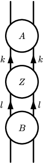
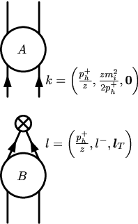
This is the case, for example, in the product between in eq. (201) — in practice it is usually not necessary to show explicitly the and integrations over the initial state partons in .
The operator is used to put eq. (203) into the form of eq. (201) in subsection V B of Ref. [33], where the remainder is shown to be power suppressed (i.e. to obey eq. (202)). A general graph, such as , containing a hard and a soft scale such as and respectively will in general contain a leading region, i.e. a part which is not power suppressed, coming from graphs which can be expressed as a graph coupled to the hard scale, the hard graph joined to a graph coupled to the soft scale, the soft graph, by 2 partons of mass much less than the hard scale [171]. Being 2PI, does not contain such graphs and therefore does not contain a leading region, i.e. it is power suppressed. This will not be the case in a general gauge, because additional gluon exchanges between the hard and soft graphs are allowed. However, it is assumed, without proof, that a suitable light-cone gauge exists such that such graphs are power suppressed. This is true for the gauge that we have been using, at least in the case that these gluons’ momenta are almost collinear with the detected hadron’s. In the leading region, lines in the hard graph will have much larger virtualities than lines in the soft graph, so lines in a 2PI graph must have similar virtualities. Therefore, because each insertion between two graphs gives a suppression of order (highest virtuality in graph below / lowest virtuality in graph above)p [33], successive insertions of in between all 2PI graphs in eq. (203) will give successive factors of this suppression leading an overall power suppression. Consequently,
| (206) |
obeys eq. (202), so may be taken to represent all higher twist terms in . All potential mass singularities in are annihilated by the insertions. All UV singularities in cancel: Acting on partons from the left with introduces a UV singularity, which is then canceled by the factors in essentially the same way as these factors remove the potential mass singularities.
The leading twist component of is therefore , which we will now factorize in order to express it in its familiar form in eq. (201).
A.2 The modern approach to factorization
The approach to factorization of Ref. [33] that we consider in this subsection is a generalization of previous approaches such as the OPE. Most importantly, it implicitly uses the cut vertices [172] and nonlocal operators [141] that were necessary in modifying the Wilson expansion in local operators on the light cone, which can be applied to e.g. the time ordered product of currents appearing in , to the time ordered product of currents appearing in , which is subtle due its nonlocal operator structure. The result that , i.e. that in eq. (201), found in Ref. [141] using an expansion in nonlocal operators, should be obtainable using the approach of Ref. [33]. Using the operator, eq. (203) may be rewritten in the form
| (207) |
In this expression, the vector
| (208) |
contains the equivalent “UV bare” (containing UV divergences) partonic processes. It is clearly free of potential mass singularities. Note that the “detected” parton is real due to the presence of on the right hand side. The UV bare FFs
| (209) |
appearing in eq. (207) describe the fragmentation of partons. Clearly, contains only and all processes contributing to the process ( is in fact a virtual parton, but its component of momentum is fixed to that of the real parton lines at the top of , while its remaining components are integrated out), and may therefore be written as a matrix element of unrenormalized operators. In a general gauge, it is given by [173, 42, 174]
| (210) |
for a quark of flavour , where is the spinor field for quarks of flavour , is the strong coupling, where are the Gell-Mann matrices, and is the field for gluons of colour charge . The operator () orders the field operators in the products in each term of the expansion of the exponential in such that an operator is always to the left (right) of any other operator with a lower (higher) value of . The superscript “” on e.g. implies that the object is unrenormalized. The expression for the gluon FF is similar, obtained essentially by replacing everywhere with the gluon field strength tensor. The Wilson lines are not present in eq. (210) in the gauge that we have been using, i.e. the exponentials are equal to unity. Their direct derivation involves going beyond the 2PI expansion in a non-trivial way. Since the UV divergences of the bare operators are subtracted by ordinary multiplicative renormalization, the renormalized FFs take the form
| (211) |
where renormalizes UV divergences in the operator in , in the standard way of operator renormalization (see e.g. [175]), and therefore introduces a dependence of on some operator renormalization scale . is non singular as parton masses vanish, as will be explicitly shown later (in the sentence containing eq. (223)). Dimensional regularization is necessary to implement the CWZ schemes, in which case will be singular as the number of dimensions approaches 4. As usual in operator renormalization, the dependence of on is governed by the renormalization group equation
| (212) |
where the components of the matrix are the relevant perturbatively calculable anomalous dimensions for the operators in , and are known as splitting functions. Therefore from eq. (211),
| (213) |
which is the DGLAP equation. In studies using the OPE, eq. (213) appears in Mellin space. where the Mellin space variable is an integer equal to the spin of the given operator in the OPE, which is equivalent to eq. (213) in space that we have just derived by applying the inverse Mellin transform of eq. (244).
We finally arrive at eq. (201) from eq. (207) by making the identity
| (214) |
where is defined such that . As for , the factorized partonic processes are also free of potential mass singularities. In practice, can be calculated as follows: We may write
| (215) |
where
| (216) |
is precisely the equivalent partonic process in which the “detected” parton is real, which is clearly free of UV divergences, but contains potential mass singularities, and
| (217) |
are the bare FFs for partons to fragment to partons. The renormalized equivalent of these FFs is
| (218) |
which is non singular as the regulator of UV singularities is removed, but is singular as any parton masses vanish. Note that and are written in Ref. [33] as and respectively. Then, instead of calculating via eq. (214), may be explicitly calculated from according to
| (219) |
where is defined such that . Equation (219), which is equivalent to eq. (65) of Ref. [33] (after expanding in ), makes it clear that the purpose of is to remove from the potential mass singularities. In other words, each potential mass singularities in is canceled by counterterms in . may be chosen, through the choice of and in eq. (218), to depend on parton masses only through mass logarithms, which will be the case for the CWZ schemes. The precise form of this (eq. (232)) will be derived later.
To summarize, and the dependence of are perturbatively calculable. The components of are the standard coefficient functions in the literature, up to electroweak couplings etc. Like the , the factorized FFs in eq. (224) are clearly universal, since all details of the initial state are contained in .
A.3 Connection with the older approach to factorization
Finally, we make some connections between the above approach and the earlier approach of Refs. [170, 43, 38]. The latter approach was formulated for the case of massless quarks only, so we will need to make some modifications to account for massive quarks as well. In addition, our definitions here of bare FFs will need to differ from the earlier approach in order to obtain reliable results. We begin with an alternative to eq. (207) which corresponds to the starting point of calculations in the literature (i.e. eq. (219)):
| (220) |
where the “bare” FF in this case is
| (221) |
which is free of UV singularities because the UV singularity introduced by acting from the left with is canceled by insertions occurring to the right, similar to the cancellation of UV singularities in discussed in the paragraph following its definition in eq. (206). We define a projection operator which projects in the same way as on parton lines above (so that ), and which projects in a similar way as on parton lines below except that, in contrast to , it becomes sufficiently suppressed for increasing momenta of these lines such that it does not introduce UV singularities. The scale at which this suppression sets in is called the factorization scale, which will be written since it will turn out to be identical to the operator renormalization scale defined above. Thus, for example, we may choose (in the case of massless quarks for simple illustration) to be given by eq. (205) multiplied by a function such that and . A more explicit definition of (or ) is not required since an implicit definition will be given later. Note that, like , is flavour diagonal. As a projection operator, , and insertion of between two 2PI graphs annihilates the potential mass singularity due to the connecting partons.
The momentum dependence of can lead to problems with gauge invariance and with rapidity divergences [176]. Such problems were not considered in Refs. [170, 43, 38], which was limited to the case of massless quarks. We will assume that some suitable choice for the remaining degrees of freedom in exists such that these problems do not arise in the case of massive quarks. Further work is needed here to prove that such a exists.
The dependence of , which was introduced in eq. (218), on is
| (222) |
which can be interpreted as the FFs for hard partons fragmenting to on-shell soft partons. Using eq. (218), we may write
| (223) |
i.e. is free of potential mass singularities because, in the operator, those potential mass singularities projected out by are identical to those projected out by . This behaviour was noted just after eq. (211). According to eqs. (201) and (219), the factorized FFs defined in eq. (211) may also be written
| (224) |
Using eq. (219), the hard partonic cross section in terms of reads
| (225) |
which is clearly free of both UV singularities and potential mass singularities. is a function only of the ratio of the component of light cone momenta of its initial and final partons, as well as of parton masses and indices. By giving this function explicitly, eq. (222) defines implicitly. The simplest possible choice for , which is the case for the CWZ schemes, is that for which the coefficients in the perturbative series for are themselves finite series in , where runs over all partons. Although the gluon mass must be zero for renormalizability, connecting gluons can be given a small mass after renormalization has been performed within the 2PI graphs. Although the perturbative approximation for fails in the numerical sense, its dependence does not, because
| (226) |
where the splitting functions
| (227) |
are clearly free of UV and potential mass singularities. This is obviously true since the perturbatively calculable must obey a similar equation to eq. (226) in order for eq. (201), in particular , to be independent of . Thus, when is chosen to depend on parton masses only through finite powers of potential mass singularities, as discussed in the paragraph preceding eq. (226), will be independent of all parton masses. The DGLAP equation, eq. (213), may be obtained from eqs. (224) and (226).
A.4 Treatment of non partonic quarks
Up to this point, all results are only valid when no parton mass is much greater than . Because the potential mass singularities of quarks that do not fall into this category are power suppressed by , where is the mass of any such quark, they must not be subtracted by a large counterterm, i.e. they must be treated differently. Thus partons must be distinguished according to how they are treated: the partons that are treated as discussed in the last 3 subsections are called active partons, while the rest, including in particular those for which , are called non partonic quarks. Note that a quark for which can be treated as either active or non partonic, since its potential mass singularities and their corresponding counterterms are not large. We define the 2PI graphs to be 2PI in non partonic quarks as well. The choice of on non partonic quarks must be such that remains both power suppressed and free of UV singularities, i.e. on non partonic quarks must be such that the arguments around eq. (206) still hold. Choosing when acting on non partonic quark lines as is done in Ref. [33] leads to UV singularities in , and therefore is not a valid possibility. One possibility which is valid is to choose when the magnitude of is large to behave in the same way on non partonic quark lines as on active quark lines, i.e. to choose eq. (205) to hold for non partonic quarks as well, thus guaranteeing the cancellation of UV divergences in , while the on non partonic quark lines vanishes as becomes small to both guaranteeing the power suppression of and ensuring no large counterterms are introduced for potential mass singularities due to non partonic quark, which are suppressed or not large. In other words, on non partonic quark lines may be chosen in a similar way to how acting on active quark lines was in the paragraph following eq. (221), except that now is replaced with another function, say, where is another arbitrary scale at which the suppression of acting on non partonic quark lines sets in, which obeys and . In this case, would no longer be a projection operator, and is now scheme and scale dependent, i.e. it depends on the number of flavours and on respectively. Neither of these two facts presents any problems. However, as noted in the paragraph preceding the paragraph containing eq. (222), introducing a momentum dependence into a projection operator can lead to problems with gauge invariance and with rapidity divergences, so further work is needed to prove that a exists for which these problems do not arise.
For now, for simplicity, to avoid possible problems with gauge invariance and with rapidity divergences, and to ensure that is free of UV singularities, we will choose on non partonic quark lines to be the same as on active quark lines (i.e. the massive quark equivalent of eq. (205)). However, in this case is no longer power suppressed. Then, in the presence of non partonic quarks, all results derived so far still hold, except that the sum over partons in all products such as that in eq. (201) includes non partonic quarks. In certain “physical” schemes, defined in subsection II.7 to be schemes such as the CWZ schemes in which no subtraction is made on quantities which are free of UV singularities, depends on non partonic quark masses only, and is singular as such masses vanish (recall from subsection A.2 that is non singular as active parton masses vanish), while is independent of non partonic quark masses. When acting on non partonic quark lines, must be chosen such that it does not introduce large counterterms to cancel power suppressed potential mass singularities, e.g. can be chosen to vanish on non partonic quark lines.
The other type of potential mass singularity that a non partonic quark contributes, namely logarithms of its mass that become singular as are absorbed into the strong coupling constant in e.g. a CWZ scheme. Note that, for active partons, for which , such logarithms are power suppressed by .
In calculations of light hadron production, it may or may not be possible to neglect the contribution of intrinsic fragmentation, namely the non partonic components in the product in eq. (201). In the case of PDFs, according to the decoupling theorem those graphs that contain a non partonic quark will be suppressed by a power of [22], which is therefore the relative error on the cross section due to the neglect of the intrinsic PDF of parton . If such a suppression occurs also for FFs then, as for PDFs, can be neglected, in which case eq. (228) implies that is determined entirely from the for . This component of describes the extrinsic fragmentation of parton . However, the results of Ref. [22] only apply to the case of local operators, such as those relevant to DIS, but not necessarily to FFs for which non local operators must be used, as was mentioned earlier. If the intrinsic fragmentation of a non partonic quark is deemed important (e.g. charm fragmentation in a 3 flavour scheme), calculations would need to be made in which acting on non partonic lines takes the required form. In the meantime, a quark whose intrinsic fragmentation is large must be treated as an active parton, with an intrinsic FF that can be fitted to experimental data as is the case for the light partons, and thus cannot be too small relative to its mass.
A.5 Matching conditions
Next we consider the relation, or matching conditions, between , and , in schemes that differ by the number of active partons. Taking all quantities above to be defined for active quark flavours and using primes to denote quantities defined with active quark flavours, eq. (211) implies that the matching conditions for FFs and coefficient functions is, respectively,
| (228) |
and
| (229) |
where is a function only of the ratio of the component of light cone momenta of its initial and final partons, as well as of parton masses and indices. Diagrammatically it is given by
| (230) |
Note that remains non singular as the regulator of UV singularities is removed, in contrast to , and, as for , contains no potential mass singularities due to active parton masses. can be chosen such that depends on non partonic quark masses only, and only through mass logarithms. This is the case in the CWZ schemes. Recall that some modification of our incomplete results in this subsection are needed to ensure that is properly power suppressed. Again, similar to above, if is chosen to have the simplest possible form as discussed in the paragraph preceding eq. (226), the only parton mass that can depend on is . Since the series for starts at , since projects out a potential mass singularity from the th quark, and since factors of contain pairs of connecting partons and therefore a product of potential mass singularities, in Mellin space and as a matrix in parton species takes the form
| (231) |
From this we obtain the simplest possible form for :
| (232) |
In practice, the are chosen such that in eq. (219) is finite in the limit that active parton masses vanish (although these limits do not of course need to be taken in the actual cross section calculations). The CWZ scheme is obtained by choosing the such that in eq. (219) reduces to the scheme for a theory with massless flavours only in the limits that active parton masses vanish and non partonic masses approach infinity (which again do not need to be taken in actual applications).
A.6 Open issues
We have given a brief summary of the current status of factorization which was developed in Ref. [33]. This approach both generalizes earlier approaches and solves a number of issues therein. However, some issues remain. In particular, the modification that we have proposed here to the behaviour of on non partonic quark lines given in Ref. [33], as well as our proposed relations between the results of Ref. [33] and those of the earlier approach of Refs. [170, 43, 38] in terms of , need more explicit study in order to ensure that there are no problems with gauge invariance or rapidity divergences, which are a general consequence of momentum dependent projection operators. Furthermore, while it has been proved that graphs in which there is an exchange between the hard and soft graphs of gluons collinear to the detected hadron are power suppressed, a proof is lacking for gluons which are not collinear.
Appendix B Leading order splitting functions
The LO coefficients of the splitting functions are given by
| (233) |
where and, for the color gauge group SU(3), and . The operation occurs often in perturbative calculations, and can be most usefully defined by its behaviour in a convolution (in which it will always appear):
| (234) |
for any functions and . Supposing that may contain a singularity as but nowhere else, eq. (234) is non singular provided is less singular than , because the quantity in square brackets in the first integral on the right hand side falls to zero as fast as in this limit. On the other hand, without the operation, eq. (234) is only non singular provided is less singular than . By choosing , removing the common factor and then replacing the lower limit of the integration on the left hand side with , we find the Mellin transform of to be
| (235) |
Transforming eq. (233) to Mellin space gives
| (236) |
where, for integer , the harmonic sum
| (237) |
Equation (237) can be analytically continued to complex [69] by making the replacement and then making the replacement in the second sum. The result is
| (238) |
This sum converges, but rather slowly. For numerical work, should be calculated using the result [69]
| (239) |
that follows from eq. (237), where should be chosen such that is large, and then calculating as an expansion in [177].
Appendix C Mellin space
Any succession of convolutions, which may be written as
| (240) |
is converted by the Mellin transform, defined by the integral transformation
| (241) |
into an analytically more manageable succession of products
| (242) |
which is most easily proved by applying the Mellin transform to an alternative form of eq. (240),
| (243) |
The Mellin transform is invertible via the inverse Mellin transform
| (244) |
where is a contour in complex space which starts from a point at , ends at a point at , and passes to the right of all poles in . According to Cauchy’s theorem, the contour may be deformed provided that it does not pass through any poles in the process. The numerical evaluation of the integration in eq. (244) converges fastest when a contour for which is used, because then falls exponentially to zero along it.
Often in a convolution of two functions,
| (245) |
the analytic Mellin transform of one of these functions, say, may not be calculable. (Note that eq. (245) includes the cases of multiple convolutions in eq. (240), since can be equated with a subset of the convolutions in eq. (240) and with the rest.) An example is the appearing in eq. (82). In this case the Mellin transform of may be performed numerically, but only after dealing with a subtlety: Equation (241) with implies that the second equality in eq. (245) has a divergent contribution proportional to whenever , if the contour is chosen as discussed at the end of the previous paragraph. However, inspection of the first equality in eq. (245) reveals that is independent of in this region. Thus in the second equality in eq. (245) must be replaced with the modified Mellin transform
| (246) |
It can sometimes happen that the analytic Mellin transform of the other function, , also cannot be obtained. Unfortunately, eq. (246) cannot be used to also calculate the Mellin transform of , because then the inverse Mellin transform does not converge: As well as eq. (246), assume a second result which is the same as eq. (246) but with and . Then eq. (245) has a divergent contribution proportional to from the region , which exists even though and . One solution is instead to approximate in space as e.g. an expansion in Chebyshev polynomials, and then analytically Mellin transform it.
Appendix D Summary of inclusive single hadron production measurements
Only , , , and data which can be reasonably reliably calculated, and which are therefore suitable for global fits, are listed here.
D.1 reactions
| Collaboration | Tagging | # | Norm. | |
| (GeV) | data | (%) | ||
| TASSO [178] | untagged | 12 | 5 | 20 |
| TASSO [113] | untagged | 14 | 10 | 8.5 |
| TASSO [113] | untagged | 22 | 1 | 6.3 |
| HRS [179] | untagged | 29 | 6 | |
| TPC [55] | l tagged | 29 | 9 | |
| TPC [55] | c tagged | 29 | 9 | |
| TPC [55] | b tagged | 29 | 9 | |
| TPC [89] | untagged | 29 | 27 | |
| TASSO [178] | untagged | 30 | 4 | 20 |
| TASSO [90] | untagged | 34 | 10 | 6 |
| TASSO [90] | untagged | 44 | 7 | 6 |
| TOPAZ [157] | untagged | 58 | 8 | |
| ALEPH [79] | untagged | 91.2 | 22 | 3 |
| DELPHI [56] | l tagged | 91.2 | 17 | |
| DELPHI [56] | b tagged | 91.2 | 17 | |
| DELPHI [56] | untagged | 91.2 | 17 | |
| OPAL [58] | u tagged | 91.2 | 5 | |
| OPAL [58] | d tagged | 91.2 | 5 | |
| OPAL [58] | s tagged | 91.2 | 5 | |
| OPAL [58] | c tagged | 91.2 | 5 | |
| OPAL [58] | b tagged | 91.2 | 5 | |
| OPAL [180] | untagged | 91.2 | 20 | |
| SLD [181] | l tagged | 91.2 | 28 | |
| SLD [181] | c tagged | 91.2 | 28 | |
| SLD [181] | b tagged | 91.2 | 28 | |
| SLD [181] | untagged | 91.2 | 28 | |
| DELPHI [182] | untagged | 189 | 3 | |
| Total | 338 |
| Collaboration | Tagging | # | Norm. | |
| (GeV) | data | (%) | ||
| TASSO [178] | untagged | 12 | 3 | 20 |
| TASSO [113] | untagged | 14 | 9 | 8.5 |
| TASSO [113] | untagged | 22 | 7 | 6.3 |
| HRS [179] | untagged | 29 | 7 | |
| MARKII [183] | untagged | 29 | 2 | 12 |
| TPC [89] | untagged | 29 | 26 | |
| TASSO [178] | untagged | 30 | 2 | 20 |
| TASSO [90] | untagged | 34 | 5 | 6 |
| TOPAZ [157] | untagged | 58 | 5 | |
| ALEPH [79, 158] | untagged | 91.2 | 18 | 3 |
| DELPHI [56] | l tagged | 91.2 | 17 | |
| DELPHI [56] | b tagged | 91.2 | 17 | |
| DELPHI [56] | untagged | 91.2 | 17 | |
| OPAL [58] | u tagged | 91.2 | 5 | |
| OPAL [58] | d tagged | 91.2 | 5 | |
| OPAL [58] | s tagged | 91.2 | 5 | |
| OPAL [58] | c tagged | 91.2 | 5 | |
| OPAL [58] | b tagged | 91.2 | 5 | |
| OPAL [180] | untagged | 91.2 | 10 | |
| SLD [181] | l tagged | 91.2 | 28 | |
| SLD [181] | c tagged | 91.2 | 28 | |
| SLD [181] | b tagged | 91.2 | 28 | |
| SLD [181] | untagged | 91.2 | 28 | |
| DELPHI [182] | untagged | 189 | 3 | |
| Total | 286 |
| Collaboration | Tagging | # | Norm. | |
| (GeV) | data | (%) | ||
| TASSO [178] | untagged | 12 | 3 | 20 |
| TASSO [113] | untagged | 14 | 9 | 8.5 |
| TASSO [113] | untagged | 22 | 9 | 6.3 |
| HRS [179] | untagged | 29 | 7 | |
| TPC [89] | untagged | 29 | 20 | |
| TASSO [178] | untagged | 30 | 3 | 20 |
| JADE [184] | untagged | 34 | 2 | 14 |
| TASSO [90] | untagged | 34 | 7 | 6 |
| TOPAZ [157] | untagged | 58 | 5 | |
| ALEPH [79, 158] | untagged | 91.2 | 18 | 3 |
| DELPHI [56] | l tagged | 91.2 | 17 | |
| DELPHI [56] | b tagged | 91.2 | 17 | |
| DELPHI [56] | untagged | 91.2 | 17 | |
| OPAL [58] | u tagged | 91.2 | 5 | |
| OPAL [58] | d tagged | 91.2 | 5 | |
| OPAL [58] | s tagged | 91.2 | 5 | |
| OPAL [58] | c tagged | 91.2 | 5 | |
| OPAL [58] | b tagged | 91.2 | 5 | |
| OPAL [180] | untagged | 91.2 | 10 | |
| SLD [181] | l tagged | 91.2 | 29 | |
| SLD [181] | c tagged | 91.2 | 29 | |
| SLD [181] | b tagged | 91.2 | 29 | |
| SLD [181] | untagged | 91.2 | 29 | |
| DELPHI [182] | untagged | 189 | 3 | |
| Total | 289 |
| Collaboration | Tagging | # | Norm. | |
| (GeV) | data | (%) | ||
| TASSO [185] | untagged | 14 | 8 | 15 |
| TASSO [186] | untagged | 14.8 | 8 | |
| TASSO [186] | untagged | 21.5 | 5 | |
| TASSO [185] | untagged | 22 | 5 | 15 |
| HRS [179] | untagged | 29 | 12 | |
| MARK II [183] | untagged | 29 | 17 | 12 |
| TPC [187] | untagged | 29 | 7 | |
| TASSO [188] | untagged | 33.3 | 7 | 15 |
| TASSO [185] | untagged | 34 | 13 | 15 |
| TASSO [186] | untagged | 34.5 | 13 | |
| CELLO [189] | untagged | 35 | 9 | |
| TASSO [186] | untagged | 35 | 13 | |
| TASSO [186] | untagged | 42.6 | 13 | |
| TOPAZ [157] | untagged | 58 | 4 | |
| ALEPH [158] | untagged | 91.2 | 16 | 2 |
| DELPHI [190] | untagged | 91.2 | 13 | |
| OPAL [58] | u tagged | 91.2 | 5 | |
| OPAL [58] | d tagged | 91.2 | 5 | |
| OPAL [58] | s tagged | 91.2 | 5 | |
| OPAL [58] | c tagged | 91.2 | 5 | |
| OPAL [58] | b tagged | 91.2 | 5 | |
| OPAL [191] | untagged | 91.2 | 16 | 6 |
| SLD [57] | l tagged | 91.2 | 9 | |
| SLD [57] | c tagged | 91.2 | 9 | |
| SLD [57] | b tagged | 91.2 | 9 | |
| SLD [57] | untagged | 91.2 | 9 | |
| DELPHI [182] | untagged | 183 | 2 | |
| DELPHI [182] | untagged | 189 | 3 | |
| Total | 252 |
| Collaboration | Tagging | # | Norm. | |
| (GeV) | data | (%) | ||
| TASSO [185] | untagged | 14 | 3 | 20 |
| TASSO [185] | untagged | 22 | 4 | 20 |
| HRS [192] | untagged | 29 | 12 | |
| MARK II [193] | untagged | 29 | 15 | |
| TASSO [188] | untagged | 33.3 | 6 | 15 |
| TASSO [185] | untagged | 34 | 6 | 20 |
| TASSO [194] | untagged | 34.8 | 9 | 9 |
| CELLO [189] | untagged | 35 | 7 | |
| TASSO [90] | untagged | 42.1 | 4 | 9 |
| ALEPH [158] | untagged | 91.2 | 16 | 4 |
| DELPHI [195] | untagged | 91.2 | 7 | |
| OPAL [58] | u tagged | 91.2 | 5 | |
| OPAL [58] | d tagged | 91.2 | 5 | |
| OPAL [58] | s tagged | 91.2 | 5 | |
| OPAL [58] | c tagged | 91.2 | 5 | |
| OPAL [58] | b tagged | 91.2 | 5 | |
| OPAL [196] | untagged | 91.2 | 12 | |
| SLD [57] | l tagged | 91.2 | 4 | |
| SLD [57] | c tagged | 91.2 | 4 | |
| SLD [57] | b tagged | 91.2 | 4 | |
| SLD [57] | untagged | 91.2 | 9 | |
| DELPHI [182] | untagged | 183 | 3 | |
| DELPHI [182] | untagged | 189 | 3 | |
| Total | 145 |
D.2 reactions
| Collaboration | Rapidity | # | Norm. | |
| (GeV) | data | (%) | ||
| BRAHMS [197] | 200 | 8 | 11,7,8(13), | |
| 7 | 2,1(3) | |||
| PHENIX [198] () | 200 | 13 | 9.7 | |
| STAR [199] () | 200 | 4 | 16 | |
| STAR [199] () | 200 | 2 | 16 | |
| STAR [116] | 200 | 10 | 11.7 | |
| Total | 44 |
| Collaboration | Rapidity | # | Norm. | |
| (GeV) | data | (%) | ||
| BRAHMS [197] | 200 | 7 | 11,7,8(13), | |
| 5 | 2,1(3) | |||
| STAR [116] | 200 | 8 | 11.7 | |
| Total | 20 |
References
- [1] R. D. Field and R. P. Feynman, Phys. Rev. D 15 (1977) 2590; Nucl. Phys. B 136 (1978) 1.
- [2]
http://en.wikipedia.org/wiki/List_of_mesonsandhttp://en.wikipedia.org/wiki/List_of_baryons. - [3] S. Albino et al., arXiv:0804.2021 [hep-ph].
- [4] D. de Florian, O. A. Sampayo and R. Sassot, Phys. Rev. D 57 (1998) 5803 [arXiv:hep-ph/9711440]; T. Hasegawa [Spin Muon Collaboration], Nucl. Phys. A 629 (1998) 273C; HERMES Collaboration, A. Airapetian et al., Phys. Rev. Lett. 92 (2004) 012005 [arXiv:hep-ex/0307064]; Phys. Rev. D 71 (2005) 012003 [arXiv:hep-ex/0407032]. D. de Florian, G. A. Navarro and R. Sassot, Phys. Rev. D 71 (2005) 094018 [arXiv:hep-ph/0504155].
- [5] M. Gronau, F. Ravndal and Y. Zarmi, Nucl. Phys. B 51 (1973) 611; European Muon Collaboration, M. Arneodo et al., Nucl. Phys. B 321 (1989) 541.
- [6] D. de Florian, Phys. Rev. D 67 (2003) 054004 [arXiv:hep-ph/0210442]; B. Jager, A. Schafer, M. Stratmann and W. Vogelsang, Phys. Rev. D 67 (2003) 054005 [arXiv:hep-ph/0211007].
- [7]
A. Deshpande, R. Milner, R. Venugopalan and W. Vogelsang,
Ann. Rev. Nucl. Part. Sci. 55 (2005) 165
[arXiv:hep-ph/0506148];
http://www.bnl.gov/eic. - [8] J. B. Dainton, M. Klein, P. Newman, E. Perez and F. Willeke, JINST 1 (2006) P10001 [arXiv:hep-ex/0603016].
- [9] B. Jager, M. Stratmann and W. Vogelsang, Phys. Rev. D 68 (2003) 114018 [arXiv:hep-ph/0309051]; Eur. Phys. J. C 44 (2005) 533 [arXiv:hep-ph/0505157].
- [10] PHENIX Collaboration, S. S. Adler et al., Phys. Rev. Lett. 91 (2003) 072301 [arXiv:nucl-ex/0304022]; PHENIX Collaboration, K. Adcox et al., Nucl. Phys. A 757 (2005) 184 [arXiv:nucl-ex/0410003].
- [11] M. Gluck, E. Reya and A. Vogt, Phys. Rev. D 48 (1993) 116 [Erratum-ibid. D 51 (1995) 1427].
- [12] K. Koller, T. F. Walsh and P. M. Zerwas, Z. Phys. C 2 (1979) 197.
- [13] E. Braaten and J. Lee, Phys. Rev. D 65 (2002) 034005 [arXiv:hep-ph/0102130].
- [14] J. w. Qiu and X. f. Zhang, Phys. Rev. D 64 (2001) 074007 [arXiv:hep-ph/0101004].
- [15] M. Hirai, S. Kumano, M. Oka and K. Sudoh, Phys. Rev. D 77 (2008) 017504 [arXiv:0708.1816 [hep-ph]].
- [16] S. D. P. Vlassopulos, Lett. Nuovo Cim. 42 (1985) 225; E. C. Katsoufis and S. D. P. Vlassopulos, Nuovo Cim. A 86 (1985) 87.
- [17] C. H. Chang, J. K. Chen, Z. Y. Fang, B. Q. Hu and X. G. Wu, Eur. Phys. J. C 50 (2007) 969 [arXiv:hep-ph/0602158].
- [18] Z. Fodor and S. D. Katz, Phys. Rev. Lett. 86 (2001) 3224 [arXiv:hep-ph/0008204]. C. Coriano and A. E. Faraggi, Phys. Rev. D 65 (2002) 075001 [arXiv:hep-ph/0106326]. R. Aloisio, V. Berezinsky and M. Kachelriess, Phys. Rev. D 69 (2004) 094023 [arXiv:hep-ph/0307279]; A. Cafarella, QCD at hadron colliders and in ultra high energy cosmic rays, Ph.D. Thesis [arXiv:hep-ph/0605241].
- [19] I. Mocioiu, Y. Nara and I. Sarcevic, Phys. Lett. B 557 (2003) 87 [arXiv:hep-ph/0301073].
- [20] F. Arleo, arXiv:0810.1193 [hep-ph].
- [21] T. Appelquist and J. Carazzone, Phys. Rev. D 11 (1975) 2856.
- [22] E. Witten, Nucl. Phys. B 104 (1976) 445.
- [23] J. C. Collins, F. Wilczek and A. Zee, Phys. Rev. D 18 (1978) 242.
- [24] P. Nason and B. R. Webber, Nucl. Phys. B 421 (1994) 473 [Erratum-ibid. B 480 (1996) 755].
- [25] T. Kneesch, B. A. Kniehl, G. Kramer and I. Schienbein, Nucl. Phys. B 799 (2008) 34 [arXiv:0712.0481 [hep-ph]].
- [26] S. Kretzer and I. Schienbein, Phys. Rev. D 59 (1999) 054004 [arXiv:hep-ph/9808375].
- [27] P. Nason, S. Dawson and R. K. Ellis, Nucl. Phys. B 327 (1989) 49 [Erratum-ibid. B 335 (1990) 260]; W. Beenakker, H. Kuijf, W. L. van Neerven and J. Smith, Phys. Rev. D 40 (1989) 54; W. Beenakker, W. L. van Neerven, R. Meng, G. A. Schuler and J. Smith, Nucl. Phys. B 351 (1991) 507.
- [28] B. A. Kniehl, G. Kramer, I. Schienbein and H. Spiesberger, Phys. Rev. D 71 (2005) 014018 [arXiv:hep-ph/0410289]; Eur. Phys. J. C 41 (2005) 199 [arXiv:hep-ph/0502194]. B. A. Kniehl, G. Kramer, I. Schienbein and H. Spiesberger, Phys. Rev. D 77 (2008) 014011 [arXiv:0705.4392 [hep-ph]];
- [29] V. N. Gribov and L. N. Lipatov, Sov. J. Nucl. Phys. 15 (1972) 438 [Erratum-ibid. 675].
- [30] L. N. Lipatov, Sov. J. Nucl. Phys. 20, 94 (1975) [Yad. Fiz. 20, 181 (1974)]; G. Altarelli and G. Parisi, Nucl. Phys. B 126, 298 (1977); Y. L. Dokshitzer, Sov. Phys. JETP 46, 641 (1977) [Zh. Eksp. Teor. Fiz. 73, 1216 (1977)]. In J. C. Collins and J. w. Qiu, Phys. Rev. D 39 (1989) 1398, the singularities at are derived diagrammatically rather than imposed by hand using the momentum sum rule.
- [31] W. J. Marciano, Phys. Rev. D 29 (1984) 580.
- [32] M. Cacciari, P. Nason and C. Oleari, JHEP 0510 (2005) 034 [arXiv:hep-ph/0504192].
- [33] J. C. Collins, Phys. Rev. D 58 (1998) 094002 [arXiv:hep-ph/9806259].
- [34] M. A. G. Aivazis, J. C. Collins, F. I. Olness and W. K. Tung, Phys. Rev. D 50 (1994) 3102 [arXiv:hep-ph/9312319].
- [35] G. Kramer and H. Spiesberger, Eur. Phys. J. C 22 (2001) 289 [arXiv:hep-ph/0109167]; 28 (2003) 495 [arXiv:hep-ph/0302081]; 38 (2004) 309 [arXiv:hep-ph/0311062].
- [36] M. Krämer, F. I. Olness and D. E. Soper, Phys. Rev. D 62 (2000) 096007 [arXiv:hep-ph/0003035].
- [37] W. K. Tung, S. Kretzer and C. Schmidt, J. Phys. G 28 (2002) 983 [arXiv:hep-ph/0110247].
- [38] W. Furmanski and R. Petronzio, Z. Phys. C 11 (1982) 293.
- [39] R. K. Ellis, Z. Kunszt and E. M. Levin, Nucl. Phys. B 420 (1994) 517 [Erratum-ibid. B 433 (1995) 498].
- [40] Yu. L. Dokshitzer, G. Marchesini and G. P. Salam, Phys. Lett. B 634 (2006) 504 [arXiv:hep-ph/0511302].
- [41] J. Blumlein and A. Vogt, Phys. Rev. D 58 (1998) 014020 [arXiv:hep-ph/9712546].
- [42] J. C. Collins and D. E. Soper, Nucl. Phys. B 194 (1982) 445.
- [43] G. Curci, W. Furmanski and R. Petronzio, Nucl. Phys. B 175 (1980) 27; W. Furmanski and R. Petronzio, Phys. Lett. B 97 (1980) 437.
- [44] R. K. Ellis, W. J. Stirling and B. R. Webber, QCD and collider physics, Camb. Monogr. Part. Phys. Nucl. Phys. Cosmol. 8 (1996) 1.
- [45] M. Stratmann and W. Vogelsang, Nucl. Phys. B 496 (1997) 41 [arXiv:hep-ph/9612250].
- [46] A. Mitov, S. Moch and A. Vogt, Phys. Lett. B 638 (2006) 61 [arXiv:hep-ph/0604053]; S. Moch and A. Vogt, Phys. Lett. B 659 (2008) 290 [arXiv:0709.3899 [hep-ph]].
- [47] G. Altarelli, R. K. Ellis, G. Martinelli and S. Y. Pi, Nucl. Phys. B 160 (1979) 301; R. Baier, K. Fey, Z. Phys. C 2 (1979) 339.
- [48] P. J. Rijken and W. L. van Neerven, Phys. Lett. B 386 (1996) 422 [arXiv:hep-ph/9604436]; P. J. Rijken and W. L. van Neerven, Phys. Lett. B 392 (1997) 207 [arXiv:hep-ph/9609379]; P. J. Rijken and W. L. van Neerven, Nucl. Phys. B 487 (1997) 233 [arXiv:hep-ph/9609377]; P. J. Rijken, PhD Thesi, Rijksuniversiteit te Leiden, March 1997; A. Mitov and S. O. Moch, Nucl. Phys. B 751 (2006) 18 [arXiv:hep-ph/0604160].
- [49]
Particle Data Group, C. Amsler et al.,
Phys. Lett. B 667 (2008) 1,
http://pdg.lbl.gov/ - [50] J. Binnewies, PhD Thesis, University of Hamburg, July 1997, DESY 97-128 [arXiv:hep-ph/9707269].
- [51] W. Furry, Phys. Rev. 51 (1937) 125.
- [52] B. Mele and P. Nason, Nucl. Phys. B 361 (1991) 626.
- [53] G. D. Lafferty, P. I. Reeves and M. R. Whalley, J. Phys. G 21 (1995) A1.
- [54]
http://durpdg.dur.ac.uk/HEPDATA/. - [55] X.-Q. Lu, PhD Thesis, Johns Hopkins University, 1986, Report No. UMI-87-07273; TPC/Two-Gamma Collaboration, H. Aihara et al., Phys. Lett. B 184 (1987) 299.
- [56] DELPHI Collaboration, P. Abreu et al., Eur. Phys. J. C 5 (1998) 585.
- [57] SLD Collaboration, K. Abe et al., Phys. Rev. D 59 (1999) 052001 [arXiv:hep-ex/9805029].
- [58] OPAL Collaboration, G. Abbiendi et al., Eur. Phys. J. C 16 (2000) 407 [arXiv:hep-ex/0001054].
- [59] S. Kretzer, E. Leader and E. Christova, Eur. Phys. J. C 22 (2001) 269 [arXiv:hep-ph/0108055].
- [60] D. de Florian, R. Sassot and M. Stratmann, Phys. Rev. D 76 (2007) 074033 [arXiv:0707.1506 [hep-ph]].
- [61] B. A. Kniehl, G. Kramer and B. Pötter, Nucl. Phys. B 582 (2000) 514 [arXiv:hep-ph/0010289].
- [62] L. Bourhis, M. Fontannaz, J. P. Guillet and M. Werlen, Eur. Phys. J. C 19 (2001) 89 [arXiv:hep-ph/0009101].
- [63] P. Chiappetta, M. Greco, J. P. Guillet, S. Rolli and M. Werlen, Nucl. Phys. B 412 (1994) 3 [arXiv:hep-ph/9301254].
- [64] ALEPH Collaboration, G. D. Cowan, SI-94-12 (1994), 27th International Conference on High Energy Physics (ICHEP), Glasgow, Scotland.
- [65] J. Binnewies, B. A. Kniehl and G. Kramer, Z. Phys. C 65 (1995) 471 [arXiv:hep-ph/9407347]; J. Binnewies, B. A. Kniehl and G. Kramer, Phys. Rev. D 52 (1995) 4947 [arXiv:hep-ph/9503464]; J. Binnewies, B. A. Kniehl and G. Kramer, Phys. Rev. D 53 (1996) 3573 [arXiv:hep-ph/9506437].
- [66] D. de Florian, M. Stratmann and W. Vogelsang, Phys. Rev. D 57 (1998) 5811 [arXiv:hep-ph/9711387].
- [67] S. Kretzer, Phys. Rev. D 62 (2000) 054001 [arXiv:hep-ph/0003177].
- [68] C. Bourrely and J. Soffer, Phys. Rev. D 68 (2003) 014003 [arXiv:hep-ph/0305070].
- [69] S. Albino, B. A. Kniehl and G. Kramer, Nucl. Phys. B 725 (2005) 181 [arXiv:hep-ph/0502188].
- [70] S. Albino, B. A. Kniehl and G. Kramer, Nucl. Phys. B 734 (2006) 50 [arXiv:hep-ph/0510173].
- [71] D. de Florian, R. Sassot and M. Stratmann, Phys. Rev. D 75 (2007) 114010 [arXiv:hep-ph/0703242].
- [72] S. Albino, B. A. Kniehl and G. Kramer, Nucl. Phys. B 803 (2008) 42 [arXiv:0803.2768 [hep-ph]].
- [73] M. Hirai, S. Kumano, T. H. Nagai and K. Sudoh, Phys. Rev. D 75 (2007) 094009 [arXiv:hep-ph/0702250].
- [74]
F. James, CERN Program Library Long Writeup D506,
http://wwwasdoc.web.cern.ch/wwwasdoc/minuit/minmain.html; F. James and M. Roos, Comput. Phys. Commun. 10 (1975) 343. - [75] R. Baier, J. Engels and B. Petersson, Z. Phys. C 2 (1979) 265.
- [76] M. Greco and S. Rolli, Z. Phys. C 60 (1993) 169 [arXiv:hep-ph/9304311]; M. Greco and S. Rolli, Phys. Rev. D 52 (1995) 3853 [arXiv:hep-ph/9409356]; M. Greco, S. Rolli and A. Vicini, Z. Phys. C 65 (1995) 277 [arXiv:hep-ph/9404228].
- [77] M. Anselmino, P. Kroll and E. Leader, Z. Phys. C 18 (1983) 307.
- [78] D. L. Jones and J. F. Gunion, Phys. Rev. D 19 (1979) 867.
- [79] ALEPH Collaboration, D. Buskulic et al., Z. Phys. C 66 (1995) 355.
- [80] ALEPH Collaboration, D. Buskulic et al., Phys. Lett. B 357 (1995) 487 [Erratum-ibid. B 364 (1995) 247]; C. Padilla Aranda, PhD Thesis, Universitat Autònoma de Barcelona, September 1995, CERN-THESIS-99-051.
- [81] OPAL Collaboration, K. Ackerstaff et al., Eur. Phys. J. C 7 (1999) 369 [arXiv:hep-ex/9807004].
- [82] OPAL Collaboration, R. Akers et al., Z. Phys. C 68 (1995) 203; DELPHI Collaboration, P. Abreu et al., Eur. Phys. J. C 6 (1999) 19.
- [83] S. Albino and R. D. Ball, Phys. Lett. B 513 (2001) 93 [arXiv:hep-ph/0011133].
- [84] S. Catani, D. de Florian, G. Rodrigo and W. Vogelsang, Phys. Rev. Lett. 93 (2004) 152003 [arXiv:hep-ph/0404240]; Nucl. Phys. Proc. Suppl. 135 (2004) 188 [arXiv:hep-ph/0406338].
- [85] E. Christova and E. Leader, arXiv:0809.0191 [hep-ph]; Eur. Phys. J. C 51 (2007) 825 [arXiv:hep-ph/0612049].
- [86] J. Blumlein, H. Bottcher and A. Guffanti, Nucl. Phys. Proc. Suppl. 135 (2004) 152 [arXiv:hep-ph/0407089]; J. Blumlein, H. Bottcher and A. Guffanti, Nucl. Phys. B 774 (2007) 182 [arXiv:hep-ph/0607200].
- [87] DASP Collaboration, R. Brandelik et al., Nucl. Phys. B 148 (1979) 189.
- [88] ARGUS Collaboration, H. Albrecht et al., Z. Phys. C 44 (1989) 547.
- [89] TPC/Two-Gamma Collaboration, H. Aihara et al., Report No. LBL-23737 and UC-34D, March 1988; TPC/Two-Gamma Collaboration, H. Aihara et al., Phys. Rev. Lett. 61 (1988) 1263.
- [90] TASSO Collaboration, W. Braunschweig et al., Z. Phys. C 42 (1989) 189.
- [91] L. Trentadue and G. Veneziano, Phys. Lett. B 323 (1994) 201.
- [92] J. C. Collins, Phys. Rev. D 57 (1998) 3051 [Erratum-ibid. D 61 (2000) 019902] [arXiv:hep-ph/9709499]; D. Graudenz, Nucl. Phys. B 432 (1994) 351 [arXiv:hep-ph/9406274]; D. Graudenz, Fortsch. Phys. 45 (1997) 629 [arXiv:hep-ph/9701334].
- [93] D. Kant, A study of the fragmentation of quarks in collisions at HERA using the H1 detector, PhD thesis, University of London (1995); P. Dixon, A study of the fragmentation of quarks in collisions at HERA, PhD thesis, University of Lancaster (1997).
- [94] H1 Collaboration, C. Adloff et al., Nucl. Phys. B 504 (1997) 3 [arXiv:hep-ex/9707005].
- [95] ZEUS Collaboration, M. Derrick et al., Z. Phys. C 70 (1996) 1 [arXiv:hep-ex/9511010].
- [96] S. Albino, B. A. Kniehl, G. Kramer and C. Sandoval, Phys. Rev. D 75 (2007) 034018 [arXiv:hep-ph/0611029].
- [97] ZEUS Collaboration, J. Breitweg et al., Phys. Lett. B 414 (1997) 428 [arXiv:hep-ex/9710011].
- [98] D. Graudenz, Fortsch. Phys. 45 (1997) 629 [arXiv:hep-ph/9701334].
- [99] J. Pumplin, D. R. Stump, J. Huston, H. L. Lai, P. Nadolsky, and W. K. Tung, JHEP 0207 (2002) 012 [arXiv:hep-ph/0201195].
- [100] H1 Collaboration, F. D. Aaron et al. , Phys. Lett. B 654, 148 (2007);
- [101] B. Brzozowska [ZEUS Collaboration], prepared for the 15th International Workshop on Deep-Inelastic Scattering and Related Subjects (DIS2007), Munich, Germany, April 2007.
- [102] R. K. Ellis and J. C. Sexton, Nucl. Phys. B 269 (1986) 445. F. Aversa, P. Chiappetta, M. Greco and J.Ph. Guillet, Phys. Lett. B 210 (1988) 225; F. Aversa, P. Chiappetta, M. Greco and J.Ph. Guillet, Phys. Lett. B 211 (1988) 465; F. Aversa, P. Chiappetta, M. Greco and J.Ph. Guillet, Nucl. Phys. B 327 (1989) 105.
- [103] R. K. Ellis, M. A. Furman, H. E. Haber and I. Hinchliffe, Nucl. Phys. B 173 (1980) 397.
- [104] Amsterdam-CERN-Nijmegen Collaboration, R. Blokzijl et al., Nucl. Phys. B 98 (1975) 401.
- [105] F. A. Ceccopieri and L. Trentadue, arXiv:0805.3467 [hep-ph].
- [106] B. A. Kniehl, G. Kramer and B. Pötter, Nucl. Phys. B 597 (2001) 337 [arXiv:hep-ph/0011155].
- [107] B. A. Kniehl, G. Kramer, and M. Maniatis, Nucl. Phys. B 711 (2005) 345 [Erratum-ibid. B 720 (2005) 231] [arXiv:hep-ph/0411300].
- [108] A. Daleo, D. de Florian, and R. Sassot, Phys. Rev. D 71 (2005) 034013 [arXiv:hep-ph/0411212].
- [109] P. Aurenche, R. Basu, M. Fontannaz, and R. M. Godbole, Eur. Phys. J. C 34 (2004) 277 [arXiv:hep-ph/0312359].
- [110] M. Fontannaz, Eur. Phys. J. C 38 (2004) 297 [arXiv:hep-ph/0410021].
- [111] P. M. Nadolsky, D. R. Stump, and C. P. Yuan, Phys. Rev. D 64 (2001) 114011 [arXiv:hep-ph/0012261].
- [112] S. Albino, B. A. Kniehl, G. Kramer and W. Ochs, Phys. Rev. D 73 (2006) 054020 [arXiv:hep-ph/0510319].
- [113] TASSO Collaboration, M. Althoff et al., Z. Phys. C 17 (1983) 5.
- [114] Yu. Dokshitzer and B. R. Webber, discussion at Third UK Phenomenology Workshop on HERA Physics, Durham, UK, 20-25 September 1998. P. Dixon, D. Kant, and G. Thompson, J. Phys. G 25 (1999) 1453; ZEUS Collaboration, J. Breitweg et al., Eur. Phys. J. C 11 (1999) 251 [arXiv:hep-ex/9903056].
- [115] A. D. Martin, R. G. Roberts, W. J. Stirling, and R. S. Thorne, Eur. Phys. J. C 23 (2002) 73 [arXiv:hep-ph/0110215].
- [116] STAR Collaboration, J. Adams et al., Phys. Lett. B 637 (2006) 161.
- [117] STAR Collaboration, B. I. Abelev et al., Phys. Rev. C 75 (2007) 064901.
- [118] M. Cacciari and S. Catani, Nucl. Phys. B 617 (2001) 253 [arXiv:hep-ph/0107138].
- [119] S. Catani and L. Trentadue, Nucl. Phys. B 327 (1989) 323.
- [120] S. Catani, M. L. Mangano, P. Nason and L. Trentadue, Nucl. Phys. B 478 (1996) 273 [arXiv:hep-ph/9604351].
- [121] D. de Florian and W. Vogelsang, Phys. Rev. D 71 (2005) 114004 [arXiv:hep-ph/0501258].
- [122] G. P. Korchemsky, Mod. Phys. Lett. A 4 (1989) 1257.
- [123] J. Kalinowski, K. Konishi, P. N. Scharbach and T. R. Taylor, Nucl. Phys. B 181 (1981) 253.
- [124] S. Albino, B. A. Kniehl and G. Kramer, Phys. Rev. Lett. 100 (2008) 192002 [arXiv:0711.1086 [hep-ph]].
- [125] R. D. Ball et al., arXiv:0808.1231 [hep-ph]; M. Ubiali, arXiv:0809.3716 [hep-ph]; J. Carnahan et al., arXiv:0810.2598 [hep-ph].
- [126] W. T. Giele and S. Keller, Phys. Rev. D 58 (1998) 094023 [arXiv:hep-ph/9803393].
- [127] D. E. Soper and J. C. Collins, arXiv:hep-ph/9411214.
- [128] J. C. Collins and J. Pumplin, arXiv:hep-ph/0105207.
- [129] R. S. Thorne et al., J. Phys. G 28 (2002) 2717 [arXiv:hep-ph/0205233].
- [130] M. Botje, J. Phys. G 28 (2002) 779 [arXiv:hep-ph/0110123].
- [131] J. Pumplin, D. R. Stump and W. K. Tung, Phys. Rev. D 65 (2002) 014011 [arXiv:hep-ph/0008191]; D. Stump et al., Phys. Rev. D 65 (2002) 014012 [arXiv:hep-ph/0101051].
- [132] J. Pumplin et al., Phys. Rev. D 65 (2002) 014013 [arXiv:hep-ph/0101032].
- [133] A. Vogt, Comput. Phys. Commun. 170 (2005) 65 [arXiv:hep-ph/0408244].
- [134]
http://wwwasdoc.web.cern.ch/wwwasdoc/shortwrupsdir/d103/top.html - [135] Numerical Recipes, Second Edition, section 5.8, William H. Press et al., Cambridge University Press (2001).
- [136] A. Hillenbrand, Measurement and simulation of the fragmentation process at HERMES, Ph.D. Thesis, DESY-THESIS-2005-035.
- [137] DELPHI Collaboration, P. Abreu et al., Phys. Lett. B 459 (1999) 397.
- [138] OPAL Collaboration, G. Alexander et al., Z. Phys. C 72 (1996) 191;
- [139] OPAL Collaboration, K. Ackerstaff et al., Z. Phys. C 75 (1997) 193; OPAL Collaboration, G. Abbiendi et al., Eur. Phys. J. C 16 (2000) 185 [arXiv:hep-ex/0002012].
- [140] CDF Collaboration, D. E. Acosta et al., Phys. Rev. D 72 (2005) 052001 [arXiv:hep-ex/0504048].
- [141] I. I. Balitsky and V. M. Braun, Phys. Lett. B 222 (1989) 123; I. I. Balitsky and V. M. Braun, Nucl. Phys. B 361 (1991) 93.
- [142] F. Anulli, arXiv:hep-ex/0406017.
- [143] Y. L. Dokshitzer, V. A. Khoze, A. H. Mueller and S. I. Troian, Basics of Perturbative QCD (Editions Frontières, Gif-sur-Yvette, 1991).
- [144] Y. L. Dokshitzer and M. Olsson, Nucl. Phys. B 396 (1993) 137.
- [145] Y. L. Dokshitzer and S. I. Troian, Proc. 19th Winter School of the LNPI, Vol. 1, p. 144 (Leningrad, 1984); Y. L. Dokshitzer and S. I. Troian, LNPI-922 preprint (1984).
- [146] V. A. Khoze and W. Ochs, Int. J. Mod. Phys. A 12 (1997) 2949 [arXiv:hep-ph/9701421].
- [147] Y. I. Azimov, Y. L. Dokshitzer, V. A. Khoze and S. I. Troian, Z. Phys. C 27 (1985) 65.
- [148] S. Albino, B. A. Kniehl, G. Kramer and W. Ochs, Phys. Rev. Lett. 95 (2005) 232002 [arXiv:hep-ph/0503170].
- [149] A. Bassetto, M. Ciafaloni, G. Marchesini and A. H. Mueller, Nucl. Phys. B 207 (1982) 189;
- [150] V. S. Fadin, Yad. Fiz. 37 (1983) 408 [Sov. J. Nucl. Phys. 37 (1983) 245].
- [151] A. H. Mueller, Nucl. Phys. B 213 (1983) 85; Nucl. Phys. B 228 (1983) 351.
- [152] J. Blumlein and V. Ravindran, Nucl. Phys. B 749 (2006) 1 [arXiv:hep-ph/0604019].
- [153] TASSO Collaboration, W. Braunschweig et al., Z. Phys. C 47 (1990) 187.
- [154] TASSO Collaboration, M. Althoff et al., Z. Phys. C 22 (1984) 307.
- [155] MARK II Collaboration, A. Petersen et al., Phys. Rev. D 37, (1988) 1.
- [156] TPC/Two Gamma Collaboration, H. Aihara et al., Phys. Rev. Lett. 61 (1988) 1263.
- [157] TOPAZ Collaboration, R. Itoh et al., Phys. Lett. B 345 (1995) 335 [arXiv:hep-ex/9412015].
- [158] ALEPH Collaboration, R. Barate et al., Phys. Rept. 294 (1998) 1.
- [159] DELPHI Collaboration, P. Abreu et al., Z. Phys. C 73 (1996) 11.
- [160] L3 Collaboration, B. Adeva et al., Phys. Lett. B 259 (1991) 199.
- [161] OPAL Collaboration, M. Z. Akrawy et al., Phys. Lett. B 247 (1990) 617.
- [162] SLC Collaboration, G. S. Abrams et al., Phys. Rev. Lett. 64 (1990) 1334.
- [163] ALEPH Collaboration, D. Buskulic et al., Z. Phys. C 73 (1997) 409.
- [164] OPAL Collaboration, G. Abbiendi et al., Eur. Phys. J. C 16 (2000) 185.
- [165] OPAL Collaboration, G. Abbiendi et al., Eur. Phys. J. C 27 (2003) 467.
- [166] S. Lupia and W. Ochs, Eur. Phys. J. C 2 (1998) 307 [arXiv:hep-ph/9704319].
- [167] C. P. Fong and B. R. Webber, Phys. Lett. B 229 (1989) 289.
- [168] H. Jung et al., arXiv:0809.0549 [hep-ph].
- [169] H. Georgi and H. D. Politzer, Phys. Rev. D 9 (1974) 416; D. J. Gross and F. Wilczek, Phys. Rev. D 9 (1974) 980; E. G. Floratos, D. A. Ross and C. T. Sachrajda, Nucl. Phys. B 129 (1977) 66 [Erratum-ibid. B 139 (1978) 545]; A. J. Buras, Rev. Mod. Phys. 52 (1980) 199; E. Reya, Phys. Rept. 69 (1981) 195; CTEQ Collaboration, R. Brock et al., Rev. Mod. Phys. 67 (1995) 157; S. Weinberg, The quantum theory of fields. Vol. 2: Modern applications, chapter 20, Cambridge University Press (1996); S. Moch and J. A. M. Vermaseren, Nucl. Phys. B 573 (2000) 853 [arXiv:hep-ph/9912355].
- [170] R. K. Ellis, H. Georgi, M. Machacek, H. D. Politzer and G. G. Ross, Phys. Lett. B 78 (1978) 281; Nucl. Phys. B 152 (1979) 285.
- [171] S. B. Libby and G. Sterman, Phys. Rev. D 18 (1978) 3252; 18 (1978) 4737.
- [172] A. H. Mueller, Phys. Rev. D 18 (1978) 3705; A. H. Mueller, Phys. Rept. 73 (1981) 237.
- [173] J. C. Collins and D. E. Soper, Nucl. Phys. B 193 (1981) 381 [Erratum-ibid. B 213 (1983) 545];
- [174] J. C. Collins, Nucl. Phys. B 396 (1993) 161 [arXiv:hep-ph/9208213].
- [175] M. E. Peskin and D. V. Schroeder, An Introduction To Quantum Field Theory, section 12.4, Addison-Wesley (1995).
- [176] J. C. Collins, Acta Phys. Polon. B 34 (2003) 3103 [arXiv:hep-ph/0304122]; J. Collins, arXiv:0808.2665 [hep-ph].
- [177] M. Abramowitz, I.A. Stegun, Handbook of Mathematical Functions with Formulas, Graphs, and Mathematical Tables, Dover Publications, New York (1965).
- [178] TASSO Collaboration, R. Brandelik et al., Phys. Lett. B 94 (1980) 444.
- [179] HRS Collaboration, M. Derrick et al., Phys. Rev. D 35 (1987) 2639.
- [180] OPAL Collaboration, R. Akers et al., Z. Phys. C 63 (1994) 181.
- [181] SLD Collaboration, K. Abe et al., Phys. Rev. D 69 (2004) 072003 [arXiv:hep-ex/0310017].
- [182] DELPHI Collaboration, P. Abreu et al., Eur. Phys. J. C 18 (2000) 203 [Erratum-ibid. C 25 (2002) 493] [arXiv:hep-ex/0103031].
- [183] MARK II Collaboration, H. Schellman et al., Phys. Rev. D 31 (1985) 3013.
- [184] JADE Collaboration, W. Bartel et al., Phys. Lett. B 104 (1981) 325.
- [185] TASSO Collaboration, M. Althoff et al., Z. Phys. C 27 (1985) 27.
- [186] TASSO Collaboration, W. Braunschweig et al., Z. Phys. C 47 (1990) 167.
- [187] TPC/Two Gamma Collaboration, H. Aihara et al., Phys. Rev. Lett. 53 (1984) 2378.
- [188] TASSO Collaboration, R. Brandelik et al., Phys. Lett. B 105 (1981) 75.
- [189] CELLO Collaboration, H. J. Behrend et al., Z. Phys. C 46 (1990) 397.
- [190] DELPHI Collaboration, P. Abreu et al., Z. Phys. C 65 (1995) 587.
- [191] OPAL Collaboration, G. Abbiendi et al., Eur. Phys. J. C 17 (2000) 373 [arXiv:hep-ex/0007017].
- [192] HRS Collaboration, P. Baringer et al., Phys. Rev. Lett. 56 (1986) 1346.
- [193] MARK II Collaboration, C. de la Vaissiere et al., Phys. Rev. Lett. 54 (1985) 2071 [Erratum-ibid. 55 (1985) 263].
- [194] TASSO Collaboration, W. Braunschweig et al., Z. Phys. C 45 (1989) 209.
- [195] DELPHI Collaboration, P. Abreu et al., Phys. Lett. B 318 (1993) 249.
- [196] OPAL Collaboration, G. Alexander et al., Z. Phys. C 73 (1997) 569.
- [197] BRAHMS Collaboration, I. Arsene et al., Phys. Rev. Lett. 98 (2007) 252001 [arXiv:hep-ex/0701041].
- [198] PHENIX Collaboration, S. S. Adler et al., Phys. Rev. Lett. 91 (2003) 241803 [arXiv:hep-ex/0304038].
- [199] STAR Collaboration, J. Adams et al., Phys. Rev. Lett. 97 (2006) 152302 [arXiv:nucl-ex/0602011].