IFT–08–11
Volume modulus inflection point inflation
and the gravitino mass problem
Marcin Badziak11 1 mbadziak@fuw.edu.pl and Marek Olechowski22 2 Marek.Olechowski@fuw.edu.pl
Institute of Theoretical Physics, University of Warsaw
ul. Hoża 69, PL–00–681 Warsaw, Poland
Abstract
Several models of inflection point inflation with the volume modulus as the inflaton are investigated. Non-perturbative superpotentials containing two gaugino condensation terms or one such term with threshold corrections are considered. It is shown that the gravitino mass may be much smaller than the Hubble scale during inflation if at least one of the non-perturbative terms has a positive exponent. Higher order corrections to the Kähler potential have to be taken into account in such models. Those corrections are used to stabilize the potential in the axion direction in the vicinity of the inflection point. Models with only negative exponents require uplifting and in consequence have the supersymmetry breaking scale higher than the inflation scale. Fine-tuning of parameters and initial conditions is analyzed in some detail for both types of models. It is found that fine-tuning of parameters in models with heavy gravitino is much stronger than in models with light gravitino. It is shown that recently proposed time dependent potentials can provide a solution to the problem of the initial conditions only in models with heavy gravitino. Such potentials can not be used to relax fine tuning of parameters in any model because this would lead to values of the spectral index well outside the experimental bounds.
1 Introduction
Mechanism of inflation has many phenomenologically desired properties. In the last couple of years a lot of attention was focused on inflationary model building motivated by the string theory. This is mainly due to a significant progress in moduli stabilization. Fluxes were used in [1] to stabilize the dilaton and the complex structure moduli. In order to stabilize the remaining volume modulus, such fluxes were supplemented by non-perturbative contributions to the superpotential and uplifting of the potential in the KKLT scenario [2]. Since the moduli fields are necessary ingredients of 4D supergravity (obtained as the low energy limit of the compactified string theory) it is very natural to ask whether they can play the role of the inflaton. With the advent of racetrack inflation [3] and its generalizations [4]-[6] it turned out that the volume modulus may be a good candidate for the inflaton. Other models of inflation driven by moduli fields were investigated e.g. in [7, 8]. In this paper we concentrate on the class of models in which effectively only one modulus - the volume Kähler modulus - plays an important role in inflation.
One of the generic properties of inflationary models based on the KKLT mechanism is the incompatibility between a high scale of inflation and a low scale of supersymmetry (SUSY) breaking. It was pointed out in [9] that the gravitino mass is typically bigger than the Hubble scale during inflation. The authors of [9] noticed that this problem could be avoided if inflation ends in a SUSY (near) Minkowski minimum11 1 In [10] it was shown that any SUSY Minkowski stationary point is stable up to possible flat directions. . However, even if such minimum exists it is still very hard to construct a model of inflation ending in that minimum. One of the main problems is that the slow-roll parameter is necessarily smaller than in models with the tree level Kähler potential and arbitrary superpotentials [11]. The situation can be improved if subleading corrections to the Kähler potential are taken into account. A model using those corrections was proposed in [11]. However, that model is quite complicated: it involves three non-perturbative gaugino condensation terms in the superpotential and requires more fine-tuning of parameters as compared to typical inflationary models.
It was found recently [12] that the Hubble scale during inflation is related to the gravitino mass also in the large volume compactification scenario . In this class of models typically which makes low-energy SUSY breaking even more problematic. A possible solution to this problem was proposed by constructing a model in which a Minkowski minimum occurs at exponentially large volume with exponentially suppressed gravitino mass [12]. However, this model suffers from the overshooting problem and requires significant amount of fine-tuning. Therefore, the problem with large gravitino mass is generic in string inflationary models and not easy to overcome.
The relation between the inflationary Hubble scale and the gravitino mass does not have to be considered problematic if we do not insist on a high scale of inflation. However, it is quite difficult to construct models with a low scale of inflation. Such models have been proposed [13, 14] but usually they require extremely small value of the slow-roll parameter which is obtained by severe fine-tuning of parameters [15]. In the present paper we concentrate on more typical models with a high scale of inflation.
The gravitino should not be very heavy if supersymmetry is to solve the hierarchy problem. On the other hand, it is well known that small gravitino mass is typically incompatible with the primordial nucleosynthesis or leads to the overclosure of the Universe (if it is stable). This is the famous gravitino problem [16, 17]. Investigation of that problem is beyond the scope of this paper. We assume that it can be solved by another sector of the theory.
In this paper we investigate models in which inflation takes place when the inflaton is close to an inflection point of the potential. Recently, models of this type gained a lot of attention in the context of brane inflation [18]-[21] as well as in the context of MSSM inflation [14, 22]. Here, we focus on inflection point inflation driven by the volume modulus. This is motivated also by the fact that a mechanism to solve the problem of the initial conditions for the inflaton in this type of models was proposed [23]. We present a few examples in which inflation starts near an inflection point and ends in a SUSY (near) Minkowski minimum. The fine-tuning of the parameters in those models is substantially weaker than in our previous model with three gaugino condensation terms [11]. We analyze also models with uplifting which do not accommodate a TeV-scale gravitino mass and compare their features to the models with a SUSY (near) Minkowski minimum.
Very important ingredients of our models are positive exponents in non-perturbative terms in the superpotential. Such terms may occur if the gauge kinetic function is a linear combination of closed string moduli [24]-[26]:
| (1) |
If gaugino condensation occurs, this results in the following non-perturbative contribution to the superpotential:
| (2) |
where is the rank of the hidden sector gauge group SU(). In the leading order approximation, the prefactor is just a constant. In general, it becomes a function of the moduli when the threshold corrections are taken into account [27, 28]. We will consider both situations: models with constant prefactors and models with moduli-dependent ones. Assuming that the dilaton is stabilized by fluxes22 2 See [29]-[32] for analysis on validity of this assumption. with the mass much bigger than the mass of we obtain the effective superpotential for the volume modulus
| (3) |
where and . In some models it may happen that is negative, and the exponent is positive. We will use such non-perturbative terms with positive exponents in models 2.1, 2.2 and 3.1 (to name the models presented in this paper we use numbers of subsections in which they are described i.e. model 2.1 is investigated in subsection 2.1 etc.). Of course, the real part of the gauge kinetic function has to be positive since it determines the physical coupling constant. Therefore, a theory with the effective superpotential (3) is reliable only in the region where . Throughout this paper we will assume that this condition is satisfied. Observe that, for a large vacuum expectation value of the dilaton, it is quite natural that the effective prefactor can be much smaller than the initial prefactor .
We should stress that gauge kinetic functions that involve more than one modulus are quite common in string theory, as was pointed out in [24]-[26]. Furthermore, in some string theories can be negative leading to positive exponents in the superpotential. This is the case for example in heterotic M-theory [33]. In the context of type IIB string theory such gauge kinetic functions can occur on magnetized D9-branes [34, 35].
Models with positive exponents were explored in a series of papers [24]-[26], where it was noticed that such forms of the superpotential may have many interesting cosmological applications. An example of such application was presented in [26] where a racetrack-type inflation model [3] was considered. It was demonstrated that adding to the superpotential a term with a positive exponent may solve the overshooting problem by increasing the height of the barrier separating the vacuum from the run-away region. Superpotentials with positive exponents were investigated also in the context of moduli stabilization [36, 37].
The rest of this paper is organized as follows. In section 2 we investigate models with two gaugino condensates in the superpotential for all possible combinations of the signs of the exponents. In some cases inflation ending in a SUSY Minkowski vacuum is possible. In other cases we have to add appropriate uplifting terms to the potential obtaining inflationary models with a heavy gravitino. In section 3 we study single gaugino condensation models with a modulus-dependent prefactor of the exponential term in the superpotential (resulting from threshold corrections to gauge kinetic functions). For simplicity we focus on a case in which such prefactor depends linearly on the volume modulus. We investigate separately the case of positive and negative exponent. Phenomenological implications of all our models are shortly discussed in section 4. In section 5 we investigate time dependent potentials proposed in [23] and discuss their impact on the fine-tuning of our models. We show that such potentials can provide solution to the problem of initial conditions in models with uplifting. We consider a simple toy-model to show that such potentials can not reduce fine-tuning of the parameters because they lead to the spectral index incompatible with the present data. In section 6 we summarize and compare the main features of our models.
2 Models with double gaugino condensation
The F-term potential in supergravity is given, in terms of the superpotential and the Kähler potential , by the following formula:
| (4) |
where .
In this section we consider models with two gaugino condensation terms in the superpotential:
| (5) |
We assume, for simplicity, that all parameters are real. The parameters and may be effective in a sense that they may depend on the vev of the dilaton as explained in the introduction (we drop the superscript “eff” for further convenience). We are interested in SUSY Minkowski minima which occur if two conditions: , , are fulfilled simultaneously. This may happen only when the parameters in the superpotential (5) fulfill the following condition:
| (6) |
Then, the SUSY Minkowski minimum is located at
| (7) |
The gravitino in such a minimum (unbroken SUSY) is exactly massless. In order to have a non-zero (but small) gravitino mass we should relax (slightly) the fine-tuning condition (6) for the superpotential parameters. Then, the minimum of the potential moves a little bit away from the position given by eq. (7). It is still supersymmetric but becomes anti de Sitter (AdS). Some mechanism is necessary to uplift it again to (almost) vanishing energy (this is the usual cosmological constant problem which we are not going to discuss). However, this uplifting is much smaller than in typical KKLT-type models. So, we will neglect it and consider models in which the superpotential parameters are (approximately) fine-tuned as in eq. (6) and with inflation ending in SUSY (near) Minkowski minima located (approximately) at given by (7).
In the present work we concentrate on models in which the real part of plays the role of the inflaton. Such inflation can be realized when the (near) Minkowski minimum and the inflection (or saddle) point, at which inflation starts, are both located at . The real part of the volume modulus at the Minkowski minimum, , must be positive. It follows from eq. (7) that is real and positive if
| (8) |
Note that the first of the above conditions is also sufficient to fulfill the condition (6) with all parameters real, as we have assumed.
The leading order Kähler potential has the following form:
| (9) |
It is easy to check that for an arbitrary superpotential with real parameters the F-term potential has some vanishing derivatives for : , . Therefore, matrix is diagonal at all stationary points satisfying . However, the sign of may change with in a way depending on details of a given model. Successful inflation in direction requires , which in our case is proportional to , to be positive for any between the inflationary inflection (or saddle) point and the Minkowski minimum, where inflation is supposed to end. In addition, one of the slow roll conditions requires that during inflation . It was shown in [11] (see also [38, 39]) that for the tree-level Kähler potential, the trace of the matrix equals at any non-supersymmetric stationary point. At any such point , and the slow roll condition is strongly violated33 3 The same problem from another point of view: at (close to) any non-supersymmetric stationary point with we find , and the potential is strongly unstable in the direction. . Successful inflation can not start near any non-supersymmetric stationary point in models with the minimal Kähler potential (9). The same arguments apply also to models in which one tries to start inflation near an inflection point. The reason is that a flat inflection point is typically either close to a flat saddle point or may be transformed to a flat saddle point by a very small change in the model parameters.
The above problem of too big negative can be solved by including some corrections to the Kähler potential. That is why we use the Kähler potential with the leading and string loop corrections [40]-[42]:
| (10) |
It is important to stress that the inclusion of the corrections to the Kähler potential implies that the potential, at this approximation, is singular at some value of at which the inverse of the Kähler metric which enters the potential,
| (11) |
is singular. As was shown in [11], the coefficients and should be positive to make the trace of the matrix positive. On the other hand, the Kähler metric has to be positive definite, so the corrections should not be too large. Therefore, the region of the potential crucial for inflation should be far away from the singularity in order to have the corrections under control.
The potential for the modulus is of the following form:
| (12) | |||||
where we set and the ellipsis stands for the terms involving and coming from the corrections to the Kähler potential. Those corrections are necessary to ensure the stability of the trajectory in the direction. We do not present explicitly the potential with the corrections since it is very complicated. Moreover, the corrections does not change qualitatively the potential in the direction except the fact that the singularity appears, as discussed before.
The potential in models with two gaugino condensates has an interesting feature: for some regions of the parameter space, there are two minima in the direction for . One of them may be a SUSY (near) Minkowski minimum. When both exponents and are negative, like in the Kallosh-Linde (KL) model [9], the second minimum is also supersymmetric and has negative energy. In models with (at least) one positive exponent, the second minimum is non-supersymmetric and may have positive energy. We will see that it is crucial for inflation whether this additional minimum is supersymmetric or not.
In the following we consider in turn models with all possible sign assignments for the exponents and .
2.1 One positive and one negative exponent
In this section we analyze a model with one positive and one negative exponent in the superpotential (5) and with the Kähler potential with the corrections (10). Let us choose , . The conditions (8) for the superpotential parameters read:
| (13) |
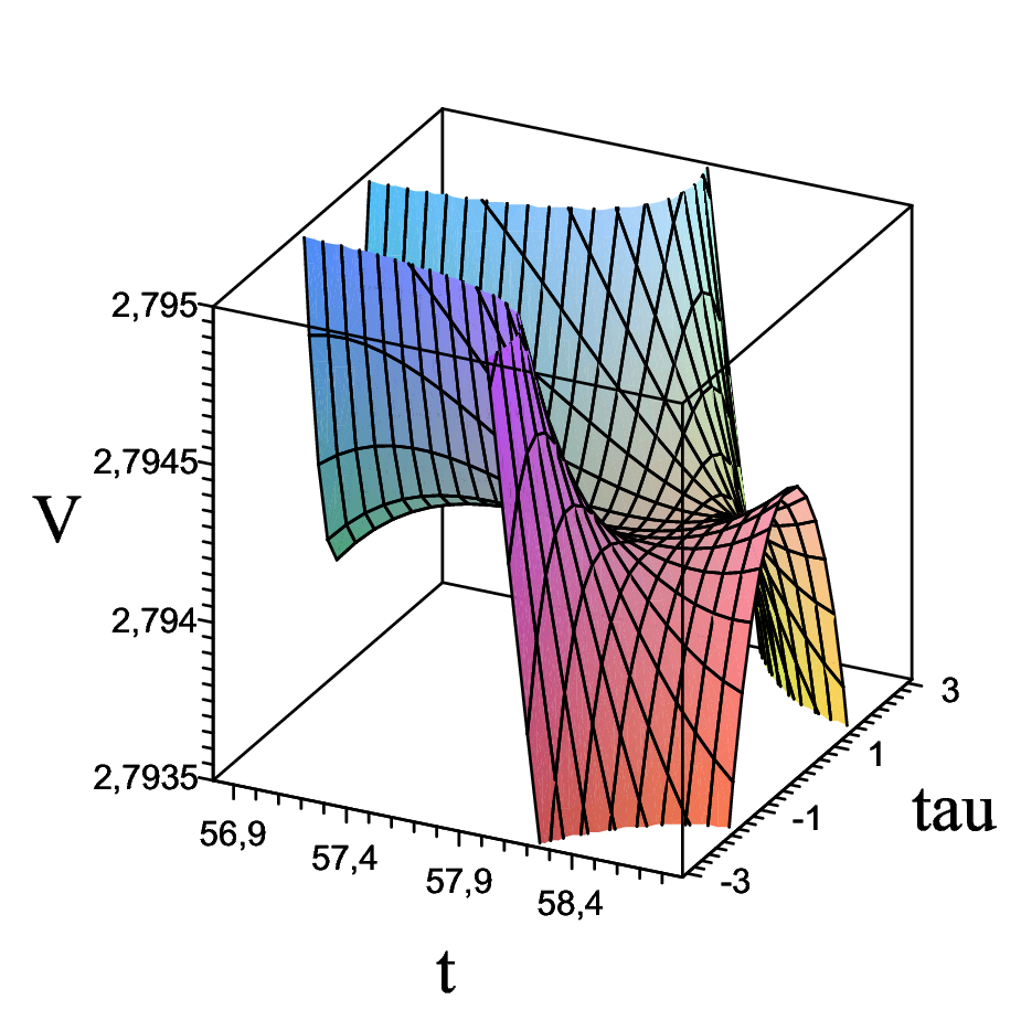
The potential for this model may have a SUSY Minkowski minimum at given by (7) and a second non-SUSY minimum at . When we decrease the ratio (keeping other parameters fixed except which is always adjusted to keep in the Minkowski minimum) this minimum becomes more and more shallow and finally disappears. Close to that transition the potential becomes very flat and allows for inflation. This is shown in figure 2. Such inflation ends at a SUSY (near) Minkowski minimum. As a result, the gravitino mass may be much smaller than the inflationary Hubble constant.
For the numerical example we choose the following set of parameters:
| (14) |
Let us first explain why is much bigger than : In order to trust the perturbative expansion of the Kähler potential, the ratios and have to be small. The amount of the corrections required to make the trace of the matrix positive at the beginning of inflation is determined by the position of the inflection point . In the model considered in this subsection , and the corrections at the Minkowski minimum are larger than at the inflection point. One can check that the distance between the Minkowski minimum and the inflection point decreases for increasing value of the ratio44 4 Changing the ratio one has also to adjust the parameter to ensure flatness of the inflection point and the parameter to keep at the Minkowski minimum. . Thus, corrections to the Kähler potential at the Minkowski minimum are smaller for larger (increasing we move away from the singularity , where the potential is not reliable).

Another feature of our numerical example is a very small value of as compared to . The reason is quite simple. In typical racetrack inflationary models both exponents and have small (negative) and similar values, because that way it is easier to obtain big enough value of at the minimum of the potential. In our model, as argued above, and should not be similar, so as can be seen from eq. (7), the only way to get is to have a large value of the ratio . Usually, very large ratios of parameters are unnatural. However, in our model the prefactor involves the exponential suppression which comes from the dilaton (which is assumed to be stabilized by fluxes), so one should expect to be much smaller than .
For the set of parameters (14), the potential in the -direction is shown in figure 2 (line (b)). Inflation takes place in the vicinity of the inflection point located at . The potential in the vicinity of that point is extremely flat, the slow roll parameter is very small: . The only non zero entry of the matrix at the inflection point is . The component of the matrix is positive for all between and , so the field may be fixed at during the whole period of inflation. Starting from the inflection point, inflaton slowly rolls down towards the SUSY (near) Minkowski minimum at . The potential has a singularity at . The ratios and have the following values: for the inflationary inflection point around and , respectively, while for the Minkowski minimum around and . Therefore, the inflationary inflection point, as well as the SUSY Minkowski minimum are still in the region of the potential where the perturbative corrections to the Kähler potential are reasonably small.
In order to find the predictions of our model we have to solve numerically equations of motion for the fields:
| (15) | |||||
| (16) |
where , . We use the number of e-folds instead of the cosmic time as the independent variable. In the above equations ′ denotes derivatives with respect to . We solve numerically these equations with the initial conditions: , and at or close to the inflection point . We find the constant value of during the whole period of inflation, as was anticipated earlier. For , after e-folds of inflation, starts to oscillate in the vicinity of the SUSY (near) Minkowski minimum, where inflation ends.
We can now ask: how much fine-tuned should be the initial conditions for the inflaton? In table 1 we show how the duration of inflation depends on the initial value of the inflaton. About 380 e-folds are obtained for a relatively wide range of between and . The fine-tuning of the initial conditions (defined as ) necessary to obtain more than e-folds of inflation is at the level of one percent for positive and about one permille for negative .
Taking into account only the flatness of the potential in the -direction one could expect that even less fine-tuning is necessary. By solving equation of motion for the inflaton (15) with one can check that e-folds of inflation is obtained for . This corresponds to . However, solving (15) independently of (16) is justified only in the region where is positive. We find that for the field becomes tachyonic (as seen in figure 2), the trajectory becomes unstable and the fields do not evolve towards the Minkowski minimum. The value of , for which the mass of the field is positive, can be enlarged by increasing the corrections to the Kähler potential. However, it is not desirable since we want to keep these corrections as small as possible. Nevertheless, the fine-tuning of the initial conditions in the inflection point inflation is much smaller than in the case of the saddle point inflation.
Finally, we comment on the fine-tuning of the parameters. We need two fine-tunings: one to obtain a light gravitino (the SUSY minimum must be near Minkowski) and second to have, for some region of , a very flat potential suitable for inflation. In both cases one has to tune appropriate combinations of all parameters. For simplicity, we tune two parameters, and , keeping other parameters fixed at some “round” values. The fine-tuning of must be at the level of in order to have a TeV-range gravitino mass (this fine-tuning can be relaxed if one wants the gravitino to be heavier). The parameter must be tuned at the level of in order to construct flat enough inflection point to obtain at least e-folds of inflation. Notice that the fine-tuning in this model is much weaker than in the triple gaugino condensation model [11], which was the first model of moduli inflation with a TeV-range gravitino mass. We recall that in the triple gaugino condensation model, flatness of the potential was obtained by fine-tuning of two parameters at the level of and . In that model two fine-tunings were needed because the diagonal and off-diagonal entries of the matrix had to be tuned separately. The reason is that in models with a SUSY Minkowski minimum the trace of the matrix cannot be large, because it is made positive only due to subleading corrections which are supposed to be small. Therefore, it is not possible to tune the smallest eigenvalue of the matrix using only one parameter, unless off-diagonal entry is suppressed by some mechanism. In all models presented in this paper, inflation takes place in the region where so the off-diagonal entry of the matrix vanishes automatically (when the parameters of the superpotential are real). Therefore, that additional fine-tuning found in [11] is not required.
2.2 Two positive exponents
Now we consider models with the superpotential (5) with both exponents positive. Without loosing generality, we consider . In such case the conditions (8) for the superpotential parameters read:
| (17) |
Inflation, that ends in a SUSY (near) Minkowski minimum, can be realized in this model if the Kähler potential (10) with the leading string corrections is used. The mechanism of inflation is very similar to the one presented in the previous subsection. For some region of the parameter space, a non-SUSY minimum with a positive cosmological constant may exist. By changing the parameter one can obtain a very flat inflection point. However, there is one important difference between this model and the previous one. Namely, in this model , so the corrections to the Kähler potential at the SUSY (near) Minkowski minimum are always smaller than at the inflationary inflection point. Therefore, one can keep the SUSY (near) Minkowski, as well as the inflationary inflection point, far away from the singularity of the potential. This also implies that the inflationary model can be constructed for arbitrary values of parameters and , which is the main advantage of this model as compared to the one with only one positive exponent. For the numerical example we choose the following set of parameters:
| (18) |

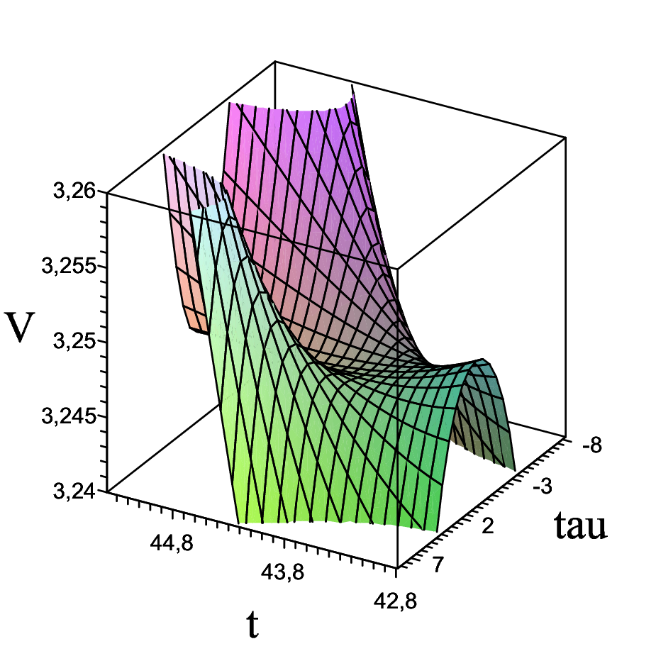
The potential in the -direction is shown in figure 4. Inflationary inflection point occurs at , where the matrix has the following entries: , . The parameter is small enough to allow for a long period of inflation. The SUSY Minkowski minimum is situated at .
Since in this model , the corrections in the region important for inflation are smaller than in a model 2.1 with one positive and one negative exponent. We find the ratios and at the inflationary inflection point equal to and , respectively, while at the Minkowski minimum and . The singularity of the potential is situated at . Therefore, inflation takes place in the region of the potential, where the perturbative expansion of the Kähler potential is justified.
In contrast to the model 2.1 with one positive and one negative exponent, in the present model with both exponents positive there is no hierarchy between the parameters and . However, both of them are very small. Similarly to the previous model, the smallness of these parameters can be explained by the exponential suppression coming from a large vev of the dilaton.
Using equations of motion (15)-(16) we evolved the fields starting from the inflection point. The evolution of the inflaton ends in the Minkowski minimum after e-folds of inflation. Similarly as in the previous model, it turns out that the inflation can be longer if it starts at some region above the inflection point. This is demonstrated in table 2. Inflation can be as long as about e-folds. The fine-tuning of the initial conditions is at the level of a few percent: . The upper bound on is not due to the potential shape in the direction55 5 By solving the equation of motion (15) for the inflaton with fixed at zero, one would obtain e-folds of inflation even for , corresponding to . but from the requirement of stability in the direction as can be seen from figure 4.
The fine-tuning of the parameters is comparable to the one in model 2.1 with one positive and one negative exponent. The parameter has to be fine-tuned at the level of to obtain gravitino mass of the order of TeV. The flatness of the potential is achieved due to the fine-tuning of the parameter at the level of .
2.3 Two negative exponents
A model with the superpotential (5) with two negative exponents is nothing else as the KL model [9]. It was shown in [11] that in such model it is not possible to realize inflation to a (near) Minkowski minimum from a saddle point. It is also not possible to have such inflation starting close to an inflection point. The reason is very simple: The second minimum in the -direction (existing in addition to the SUSY Minkowski one) is supersymmetric and has negative value of the potential. It can not be deformed to an inflection point with positive energy by any changes of the parameters if both exponents and remain negative. Thus, to realize inflation in the KL model one has to add some uplifting potential. One uplifts the SUSY AdS minimum to a (near) Minkowski one and the second minimum to an inflection (or saddle) point. Such models were investigated for example in [43]. Unfortunately, in models with uplifting the gravitino mass is bigger than the Hubble constant during inflation and the clash between light gravitino and high scale inflation appears. Nevertheless, we investigate in some detail also such model in order to compare its features, for example fine-tuning of the parameters and initial conditions, with other models with two gaugino condensates.
Following [43], we add to the potential (12) the following uplifting term:
| (19) |
The uplifting gives positive contribution to the trace of the matrix and it is not necessary to add any corrections to the Kähler potential. Moreover, corrections of the form (10), when taken into account, change the results only slightly, so in our numerical calculations we use the leading order Kähler potential (9).
The uplifting term (19) does not significantly change the positions of the stationary points of the potential. Therefore, the position of the inflationary inflection point can be well approximated by that of the SUSY Minkowski minimum (7):
| (20) |
Without loosing generality, we consider . Therefore, the parameters in this model should satisfy the conditions (8):
| (21) |
Two tunings of the parameters are necessary: one to get (almost) vanishing vacuum energy and another to obtain a sufficiently flat inflection point. Technically we choose to tune and with other parameters fixed. However, it turns out that those other parameters also play an important role. They influence the height of the barrier separating the Minkowski minimum from the run-away region at large values of the volume . There are regions in the parameter space for which inflation lasts long enough but at the end the inflaton runs away to infinity instead of oscillating around the vacuum at finite . We found that the barrier height grows with increasing and/or decreasing when the value of the potential at the inflection point is kept fixed (in order to stay in agreement with COBE normalization).

For the numerical example we choose the following set of parameters:
|
|
(22) |
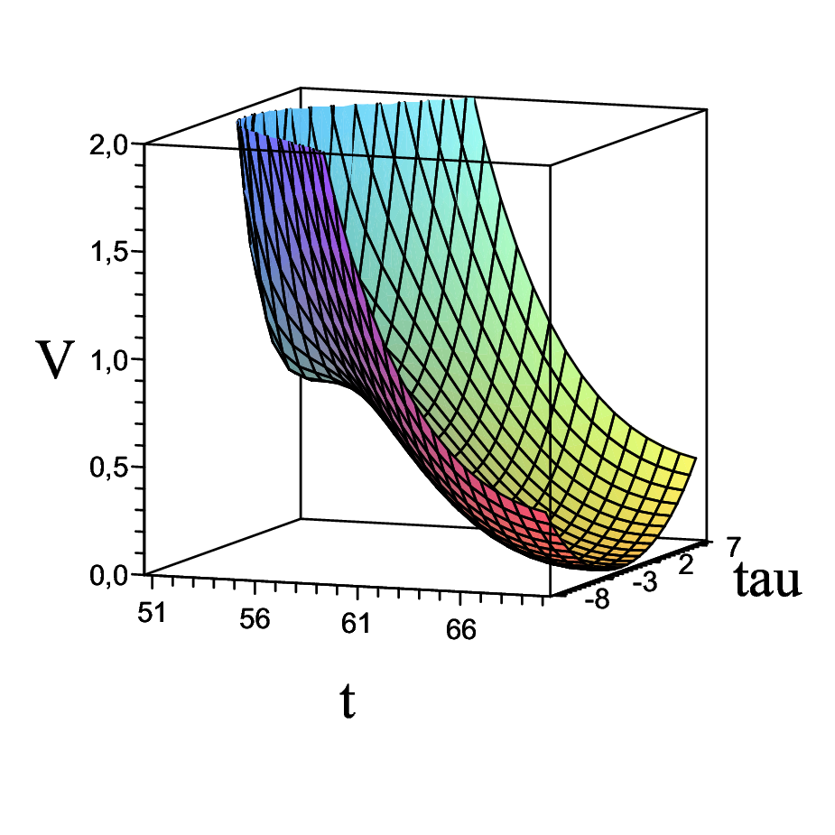
The potential in the -direction before and after uplifting is shown in figure 6. The inflationary inflection point is generated by uplifting of the minimum at smaller volume and is situated at . At this point, the only non-vanishing entry of the matrix is . Notice that the trace of the matrix is much larger than in models 2.1 and 2.2 with the SUSY (near) Minkowski minima. The reason is that a large positive contribution to the trace of the matrix is generated by a large uplifting term. At the same time, such large uplifting generates a large gravitino mass. In our example the gravitino mass at the vacuum is about GeV which is several orders of magnitude more than in typical models with low scale SUSY breaking. The Minkowski vacuum occurs at . We find a very small value of at the inflection point. In this model is a minimum in the -direction for an arbitrary value of , as can be seen in figure 6.

Solving numerically the equations of motions (15)-(16) with the initial conditions exactly at the inflection point , we obtain about e-folds of inflation. Starting from some region above the inflection point one can obtain longer period of inflation, in some cases exceeding e-folds (see table 3). It can be seen from figure 6 that the value of the potential in the vicinity of the inflection point is bigger than the height of the barrier separating the vacuum from the run-away region. Nevertheless, inflation ends with the inflaton oscillating around the vacuum (see figure 7). The overshooting does not occur due to the Hubble friction. Our numerical example was chosen in such a way that the height of the barrier is close to the minimal one necessary for protecting the inflaton from running away to infinity. The reason is that with such choice we minimize the necessary fine-tuning of parameters. We explain this point below.
In the presented example the parameter has to be fine-tuned at the level of to provide more than e-folds of inflation. Moreover, in contrast to models with the SUSY (near) Minkowski minimum, how much fine-tuning of the parameter is required depends quite strongly on other parameters of the model. We found that the fine-tuning of becomes stronger when one decreases the ratio and/or increases the ratio . As we mentioned before, these two ratios control also the height of the barrier that protects the Minkowski vacuum from overshooting. Therefore, the fine-tuning of the parameter (responsible for the flatness of the potential) is related to the height of this barrier. More fine-tuning is required when the barrier is higher. The fine-tuning at the level of is the minimal one which allows the inflaton to finish its evolution in the vacuum at finite . The height of the barrier influences in a similar way also the fine-tuning of the initial conditions: the fine-tuning becomes stronger for higher barrier. Unfortunately, even for the lowest possible barrier the fine-tuning is much stronger than in models with SUSY (near) Minkowski minima. For our numerical example in order to obtain at least 60 e-folds of inflation the initial conditions must satisfy .
The relation between the fine-tuning (of parameters and initial conditions) and the height of the barrier separating the vacuum from the run-away region can be explained by the following reasoning. The size of the region from which inflation can start and last more than e-folds, depends on the distance (before uplifting) between the minimum and the maximum that generate inflection point after uplifting of the potential. If we insist on the existence of a high barrier, the value of the potential before uplifting at the maximum should be much smaller than zero. This follows from the fact that the uplifting term (19) lifts much more strongly this maximum than the region of the potential from which the barrier arises. On the other hand, lowering the maximum (before uplifting) implies that it becomes closer to the minimum from which inflection point is generated after uplifting. Therefore, the size of the region from which inflation can start becomes smaller. Notice that for smaller region of the flat potential the slow-roll parameter (which measures the flatness of the potential) has to be smaller than in the case of larger in order to obtain the same number of e-folds. This is because the inflaton has to move slower if the region where slow-roll conditions are satisfied is smaller. Thus, for smaller values of the parameter (which is responsible for small value of ) has to be more fine-tuned. In the case when the value of the potential at the maximum (before uplifting) is positive, the distance to the minimum is larger and less fine-tuning of the parameter is needed. However, the price of this smaller fine-tuning is a very low barrier that protects the inflaton from runaway to infinity. Finally, we point out that the above reasoning does not depend on a specific form of the potential. Therefore, it applies to all other models where uplifting generates simultaneously inflationary inflection point and the Minkowski minimum (e.g. to the model discussed later in subsection 3.2).
3 Models with single gaugino condensation and threshold corrections
In this section we discuss models with only one gaugino condensate. It is known that superpotential (5) with set to zero is not suitable for describing inflation even with nonstandard Kähler potential. Therefore, we assume that the threshold corrections introduce some field dependence of the prefactor of the gaugino condensation term. The simplest such superpotential reads
| (23) |
This kind of superpotential with was considered for example in [44] but in that case inflation does not work as will be explained later. For the superpotential (23) depends only on 4 parameters. This is one parameter less than in models with two gaugino condensates considered in section 2. Nevertheless, also in this case a SUSY Minkowski minimum exists due to a -dependent prefactor if the superpotential parameters satisfy the following condition
| (24) |
The position of that minimum is given by
| (25) |
and is real for real parameters in (23). Similarly to the case considered in the previous section, potential with the corrections to the Kähler potential is very complicated. Therefore, we present only the leading part of the potential for the modulus :
| (26) |
where we set because the axion may be fixed to zero during and after inflation. The ellipsis stands for subleading terms involving and , which do not change qualitatively the features of the potential in the direction. In the following subsections we will investigate models with two possible signs of the exponent.
3.1 Positive exponent
Let us start with the model with positive exponent, , in the superpotential (23). In order to ensure that the volume at the SUSY Minkowski minimum (25) is positive, , the parameters have to satisfy (so, for positive , different signs of and are required). The parameter is fixed by the condition (24) to ensure existence of a SUSY Minkowski minimum. One can show that the slow-roll parameters depend on , and only through the combination . So, this combination is effectively the only free parameter in the class of models considered in this subsection. However, even though there is so little freedom in the parameter space, slow-roll inflation can be realized. Again, the key property of the potential, that allows for inflection point inflation ending in a SUSY (near) Minkowski minimum, is the existence of a non-SUSY minimum for some region of the parameter space. Such a minimum exists for sufficiently large values of the ratio . Choosing slightly smaller than the critical value for which such minimum disappears, one obtains a very flat inflection point, where inflation can take place. To ensure that at this inflection point the mass squared of the field is positive, one has to turn on the corrections to the Kähler potential (10). For the numerical example we choose the following set of parameters:
|
|
(27) |
The shape of the potential in the -direction is similar to that for the model 2.2, shown in figure 4. In the present case the inflationary inflection point occurs at where the only non-vanishing entry of the matrix is and the parameter is very small: . The position of the SUSY (near) Minkowski minimum, where inflation ends, is found to be , while the singularity of the potential is situated at . This singularity is not very close to the region crucial for inflation, so one may expect that the corrections to the Kähler potential are not very large. To check this we compute the ratios and . For the inflationary inflection point they are, respectively, around and . Since in this model , the corrections at the Minkowski minimum are smaller. For our numerical example they are around and . Similarly to other models with SUSY (near) Minkowski minima, we can conclude that the inflation takes place in the region of the potential where the subleading corrections are still reasonably small.
Integrating numerically the equations of motion (15)-(16) with the initial conditions , , we obtain inflation which after about e-folds ends in the SUSY Minkowski minimum. Table 4 shows how much longer inflation can be if it starts at some region above the inflection point. The maximal duration of inflation is of about e-folds. The fine-tuning of the initial conditions is at the level of a few percent (). For the potential is unstable in the direction66 6 Ignoring such instability in the direction, and taking into account only the -dependence of the potential, one would find long enough inflation even for corresponding to the fine-tuning of the initial conditions at the level of ten percent: . (its 3D shape close to the inflection point is very similar to that shown in figure 4). This kind of behavior is generic for models where the positivity of the matrix trace is obtained due to the subleading corrections to the Kähler potential.
The fine-tuning of the parameters is similar to those in other models with SUSY Minkowski minima (models 2.1 and 2.2 discussed in the previous section). The parameter has to be fine-tuned at the level of to obtain gravitino mass of the order of TeV. The flatness of the potential, which is enough to provide e-folds of inflation, is achieved due to the fine-tuning of the combination at the level of .
3.2 Negative exponent
We now discuss a model with the superpotential (23) but for negative exponent: . In this case one cannot realize inflection point inflation that ends in the SUSY Minkowski minimum. The reason is the same as for the KL model of subsection 2.3. The second minimum in the -direction (existing in addition to the SUSY Minkowski one) is supersymmetric, has negative value of the potential and can not be deformed to an inflection point with positive energy by any changes of the parameters , and . Inflation can be realized if we add to the potential (26) the uplifting term (19) . Similarly as in the KL model considered in subsection 2.3, we use the Kähler potential in the leading approximation (9). The model is constructed in a similar fashion as the one proposed in [43]. For some region of the parameter space the potential (26) without uplifting (for ) has two AdS local minima. The minimum at larger volume is deeper than the one at smaller volume. The uplifting term (19) is used to lift both minima to dS space. The value of is chosen in such a way that the minimum at larger volume has positive but almost vanishing cosmological constant. The minimum at smaller volume is more strongly lifted and acquires a large cosmological constant. It is also more strongly lifted than the local maximum separating both minima. So, for strong enough lifting, this local maximum and the minimum at smaller volume may disappear. With appropriate tuning of the parameters one can obtain a very flat inflection (or saddle) point. The position of such inflationary inflection point can be well approximated by the formula for the position of the SUSY Minkowski minimum (25):
| (28) |
Parameters and should have different signs in order to avoid too small, or even negative, .
For the numerical example we choose the following set of parameters:
| (29) |
The shape of the potential (26) before and after uplifting is quite similar to that shown in figure 6 for the KL model. The inflationary inflection point, generated by the uplifting of the minimum at smaller volume, is situated at . At that point the only non-vanishing entry of the matrix is . The second slow roll parameter at the inflection point is very small: . The (near) Minkowski vacuum is situated at . The corresponding gravitino mass is large, about GeV. The barrier, that separates the vacuum from the run-away region, occurs at . In this model is a minimum in the -direction for any value of (the 3D shape of the potential in the region important for inflation is very similar to that for the KL model shown in figure 6).

Solving numerically the equations of motion (15)-(16) with the initial conditions , , we obtain about 134 e-folds of inflation after which the inflaton oscillates around the vacuum (see figure 8). Notice that due to Hubble damping the inflaton does not overshoot the vacuum, even though the potential barrier is lower than the height of the inflationary inflection point. Table 5 shows that, starting the evolution of the inflaton from some region above the inflection point, one can obtain up to about e-folds of inflation
Let us now discuss fine-tuning of this model. In the presented example the parameter has to be fine-tuned at the level of to obtain at least e-folds of inflation. However, it turns out that the degree of fine-tuning depends on the ratio . Stronger fine-tuning is needed for larger values of . We recall that this ratio regulates also the height of the barrier that separates the vacuum from the decompactification region. Therefore, the fine-tuning required to obtain long lasting inflation is strictly related to the height of this barrier. For example, for the fine-tuning of at the level of would be enough to obtain more than e-folds of inflation. However, as we mentioned before, for the barrier is too small and the inflaton runs away to infinity. Numerical calculations show that for the minimal height of the barrier necessary to protect the inflaton from overshooting the vacuum, the fine-tuning of the parameter is at the level of .
In the presented example the fine-tuning of the initial conditions required to obtain more than e-folds of inflation equals , as seen from table 5. This fine-tuning could be relaxed even by a few orders of magnitude for smaller values of : for example, for . However, smaller values of are not allowed because of the overshooting problem. The above relations between the height of the barrier and the strength of fine-tuning can be explained by the reasoning presented at the end of subsection 2.3.
4 Experimental constraints and signatures
We now compare predictions of our models to cosmological measurements. First of all, we calculate the amplitude of density perturbations [45]:
| (30) |
where is the COBE normalization scale which leaves the horizon approximately e-folds before the end of inflation and is the amplitude of the scalar perturbations given, in the slow-roll approximation, by the following formula:
| (31) |
In all models presented in this paper the parameters were chosen in such a way as to generate the density perturbations with the amplitude consistent with COBE measurements.
Secondly, we analyze the spectral index:
| (32) |
where the last approximation comes from the fact that this quantity is evaluated at horizon crossing which implies . Approximate analytical formula for the spectral index in models of inflation starting from an inflection point was derived in [43] (see also [20, 22, 23]):
| (33) |
where is the total number of e-folds during inflation starting exactly at the inflection point while is the number of e-folds between the time when a given scale crosses the horizon and the end of inflation. We are interested in the value of at the COBE normalization scale corresponding to (the exact value of at the COBE normalization scale depends on the reheating temperature which is model dependent). In figure 9 we show that the numerically found values of the spectral index in all models presented in this paper are in a good agreement with the approximate formula (33). The 5-year WMAP result [46], , slightly favours models with smaller values of (with an exception of quite unnatural situation when is very close to ). Models with very small slope of the potential at the inflection point have large and the spectral index which can be more than below the central WMAP value. We checked numerically that the spectral index does not depend significantly on the initial conditions. This is rather intuitive because, when the inflaton starts at some very flat region above the inflection point, it approaches that inflection point with a very small velocity. Therefore, the time dependence of the inflaton field below the inflection point is almost the same as in the case when it starts at rest exactly at the inflection point, and the COBE normalization scale corresponds to almost the same value of the inflaton.

For each model considered in this paper there is a region of the corresponding parameter space for which the period of inflation starting exactly at the inflection point is shorter than e-folds while it is longer than e-folds when the inflaton starts above the inflection point. However, such parameters give the spectral index at the COBE scale bigger than unity. This follows from the fact that in such cases the COBE scale crosses the horizon when the inflaton is above the inflection point where the parameter (which determines the value of the spectral index) is positive. Therefore, in order to be consistent with the data, at least e-folds have to be generated when the inflaton is below the inflection point.
The tensor to scalar ratio depends mainly on the value of the slow-roll parameter at the inflationary inflection point, . So, in models with the SUSY (near) Minkowski minimum is bigger than in more fine-tuned models with uplifting. Nevertheless, in all models discussed in this paper, as is typical for string-inspired inflation77 7 See, however, [47] and [48] for recent proposals for generating observable gravity waves within string theory. , the value of is many orders of magnitude below the sensitivity of near future experiments. We found also that the running of the spectral index in inflection point inflation is typically of the order of so it is also negligible from the observational point of view.
5 Fine tuning and time dependent potentials
The authors of [23] postulate the existence of a time-dependent part of the potential, that is an increasing function of the volume modulus , as a possible solution to the problem of initial conditions for the inflaton in models of inflection point inflation. They argue that this kind of potential can be generated in higher dimensional models by (0+p)-branes which are point-like objects from the 4D point of view and wrap p-cycles in the internal manifold88 8 This scenario is even more attractive because, as it was argued in [49], it leads to formation of giant spherically symmetric overdense regions in the observed part of the Universe which in principle could be detected. . Using the number of e-folds instead of the cosmic time we can write such correction to the potential in the following form:
| (34) |
where is a constant of order one and is the initial density of (0+p)-branes. For this is indeed an increasing function of the volume modulus . The time-dependence of this potential is due to the expansion of the Universe which decreases the matter density. If the initial density of (0+p)-branes is large enough, the minimum of the full potential is located at some value of smaller than . We want to solve the initial conditions problem, so we do not assume that the initial value of the inflaton is very close to that minimum. Thus, for early times the inflaton oscillates around a time-dependent minimum of the full potential. Two things happen for increasing time. First: the minimum of the full potential moves towards larger values of . Second: the amplitude of the inflaton oscillations decreases due to the Hubble friction. If the initial value of the inflaton field is not too far away from the initial position of the minimum of the full potential, those oscillations may be damped very strongly before the minimum of the full potential moves to larger than the position of the inflection point of the time-independent part of the potential, . In such a case the volume modulus moves together with the minimum of the full potential towards larger values until it reaches a position very close to the inflection point where it stops tracking the time-dependent minimum. Then the usual period of slow-roll inflation begins.
This mechanism does not solve the problem of the initial conditions in models with SUSY (near) Minkowski minima because typically the potential becomes unstable in the -direction if we move too far above the inflection point. On the other hand, it works very well in models with uplifting. It is shown in tables 7 and 7 that in both models with uplifting presented in this paper even small amount of the initial density of (0+p)-branes is sufficient to solve the initial conditions problem.
In [23] it was argued that the potential (34) can also significantly reduce the fine-tuning of the parameters that are responsible for the flatness of the potential. The argument used by the authors of [23] was that one can obtain more than e-folds of inflation even if the inflection point is not flat at all. However, in what follows we show that such case is ruled out by the present experimental constraints on the spectral index.
When the inflection point is not fine-tuned to be flat, inflation may take place only when the inflaton moves together with the minimum of the full potential. In order to obtain more than e-folds of this inflationary phase the inflection point and the Minkowski vacuum have to be situated at very large values of . Moreover, the Hubble parameter decreases significantly during the evolution of the inflaton, so this is not a standard quasi-exponential inflation but rather a power law one:
| (35) |
It can be easily shown that the power exponent is related to the Hubble parameter:
| (36) |
where prime denotes derivative with respect to number of e-folds . In power law inflation the spectral index is given by [50]:
| (37) |
In order to be compatible with the data should be rather large. For example requires . In order to estimate , we consider a toy-model with the following potential:
| (38) |
The first term simulates a time-independent part of the potential. The second term is the time-dependent potential (34) with and . The position of a time-dependent minimum reads:
| (39) |
Therefore, the value of the potential (38) at a time-dependent minimum is given by:
| (40) |
In order to find the power exponent one needs (see eq. (36)). Assuming that the Hubble parameter changes mainly due to the change of the potential energy of the inflaton and not due to the change of its kinetic energy, the following relation holds:
| (41) |
Hence, using (36) and (40), we obtain the following exponent of power law inflation
| (42) |
We have calculated numerically exponent for several values of parameters and . The results are in a very good agreement with the above approximate formula. The tree-level potentials as well as the uplifting terms in models 2.3 and 3.2 behave like for small . Therefore, in those models exponent equals approximately , or for , or , respectively. We confirmed these results by our numerical analysis. Such values of the exponent are too small to give a realistic model of power law inflation (for there is no inflation at all because in this case .) There are two reasons: First, inflation with so small exponents should be very long in order to produce at least 60 e-folds. This could be achieved only for a very unnatural choice of the parameters. Second, such small values of lead to values of the spectral index well outside experimental bounds.
Using eqs. (37) and (42) we find that the spectral index for inflation driven by potential (38) reads
| (43) |
It can be in the range only if . In the mechanism proposed in [23] the biggest possible value of equals 3 (for ). The period of inflation with the inflaton tracking the time-dependent minimum of the potential gives much too small values of the spectral index. Thus, the COBE normalization scale must correspond to that part of inflation when the inflaton is close to a very flat inflection point. We conclude that the mechanism proposed in [23] can not solve the problem of fine-tuning of the parameters of the potential. It can solve only the problem of the fine-tuning of the initial condition.
6 Discussion and conclusions
We considered five models in which the volume modulus plays the role of the inflaton. In each of them inflation takes place in the vicinity of an appropriately flat inflection point of the potential. Those models may be divided into two classes. In the first class (models 2.1, 2.2 and 3.1) inflation ends in a SUSY (near) Minkowski minimum. In this class of models the corrections to the Kähler potential are necessary to realize inflation. If a SUSY (near) Minkowski minimum occurs at smaller volume than an inflationary inflection point (as in model 2.1), larger amount of corrections are required than in the opposite case (models 2.2 and 3.1). Nevertheless, in all models the corrections are small enough to trust the perturbative expansion of the Kähler potential. In the second class (models 2.3 and 3.2) inflation ends in a vacuum obtained by uplifting of some deep AdS SUSY minimum. The main phenomenological difference between those classes is the relation between the gravitino mass and the Hubble constant during inflation. In the first class the gravitino mass may be orders of magnitude smaller while in the second class it is bigger than the Hubble constant. So, only in models of the first class a light gravitino (e.g. with mass in the TeV range) is compatible with high scale (e.g. GUT scale) inflation.
The structure of the superpotential decides to which class a given model belongs. The first class contains models in which at least one gaugino condensation term has a positive exponent. Models with only negative exponents, like e.g. the KL-type models, are in the second class and can not accommodate the gravitino mass much smaller than the inflationary Hubble constant.
From a technical point of view, the crucial difference between the models from different classes is the structure of the potential. In each case the parameters may be chosen in such a way that the potential has a SUSY Minkowski minimum. The potential has (at least for some range of parameters) also the second minimum. This second minimum is supersymmetric in models with only negative exponents in the nonperturbative terms in the superpotential. It is non-supersymmetric when at least one of the gaugino condensation term has a positive exponent. Only those non-supersymmetric minima may be deformed into inflection points with a positive value of the potential, keeping the SUSY Minkowski minimum intact.
There is another interesting difference between the two classes of models. All models require some amount of fine-tuning of the parameters and the initial conditions to produce long enough inflation99 9 The fine-tuning of the parameters in the context of inflection point brane-antibrane inflation [19] was analyzed in [51]. The problem of initial conditions in that context was investigated in [52] . However, models with only negative exponents (and uplifting) need much stronger fine-tuning than models with at least one positive exponent (and no uplifting). In the latter models, the fine-tuning of the parameters is typically at the level of . The fine-tuning of the initial conditions for the inflaton field is at the level of a few percent. Models with only negative exponents require much stronger fine-tuning: about for the parameters and for the initial conditions. Such substantial differences in fine-tuning are related to the overshooting problem. In models with only negative exponents, the barrier which protects from overshooting the vacuum is generated by the uplifting. Typically the uplifting in the region of the barrier is smaller than in the region of the vacuum or the inflection point. As a result the height of the barrier is much smaller than the height of the inflection point at which inflation starts. Additional fine-tuning of the parameters (additional factor of order ) is necessary to get a high enough barrier. On the other hand, in models of the first class, a term in the superpotential with a positive exponent automatically produces a high barrier.
The difference in the fine-tuning of the initial conditions is not as large as the difference in the fine-tuning of the superpotential parameters. The initial conditions in models with only negative exponents must be fine-tuned (only) about 10 times stronger than in models with at least one positive exponent. Moreover, only in models with all negative exponents the initial conditions problem can be solved by the mechanism proposed in [23].
Finally, we should also mention that technically it is possible to construct inflationary models ending in the SUSY (near) Minkowski minimum with single gaugino condensate and a negative exponent if we allow for much more complicated function of which stands in front of the exponential term in the superpotential (e.g. containing 4-th or higher powers of ). However, we do not discuss this kind of models in detail since they seem to be quite unnatural.
To summarize let us recall briefly advantages and disadvantages of both classes of models of inflection point inflation. Models with only negative exponents in the nonperturbative terms in the superpotential require strong uplifting and so have the gravitino mass larger than the Hubble constant during inflation. The fine-tuning of parameters in those models is about 3 orders of magnitude stronger than in other models. The fine-tuning of the initial conditions is also stronger but this problem can be solved by appropriate time dependent contributions to the potential. Models with at least one positive exponent in gaugino condensation terms do not require strong uplifting and as a result may accommodate the gravitino several orders of magnitude lighter than the inflationary Hubble scale. The fine-tuning of the parameters is typical for inflation (and much weaker than in models with only negative exponents). The necessary fine-tuning of the initial conditions is at the level of a few percent but can not be made weaker by the mechanism of [23]. Corrections to the lowest order Kähler potential are necessary in those models in order to have an inflection point stable in the axion direction. The size of such corrections must be bigger than some minimal value but one can argue that they are still reasonably small.
Acknowledgments
Work partially supported by the UE 6th Framework Programs MRTN-CT-2004-503369 “Quest for Unification” and MTKD-CT-2005-029466 “Particle Physics and Cosmology: the Interface”.
References
- [1] S. B. Giddings, S. Kachru and J. Polchinski, Hierarchies from fluxes in string compactifications, Phys. Rev. D 66 (2002) 106006 [arXiv:hep-th/0105097].
- [2] S. Kachru, R. Kallosh, A. Linde and S. P. Trivedi, De Sitter vacua in string theory, Phys. Rev. D 68 (2003) 046005 [arXiv:hep-th/0301240].
- [3] J. J. Blanco-Pillado, C. P. Burgess, J. M. Cline, C. Escoda, M. Gomez-Reino, R. Kallosh, A. Linde, F. Quevedo, Racetrack inflation, JHEP 0411 (2004) 063 [arXiv:hep-th/0406230].
- [4] A. Westphal, Eternal inflation with alpha’ corrections, JCAP 0511, 003 (2005) [arXiv:hep-th/0507079].
- [5] P. Brax, A. C. Davis, S. C. Davis, R. Jeannerot and M. Postma, D-term Uplifted Racetrack Inflation, JCAP 0801 (2008) 008 [arXiv:0710.4876 [hep-th]].
- [6] J. J. Blanco-Pillado, C. P. Burgess, J. M. Cline, C. Escoda, M. Gomez-Reino, R. Kallosh, A. Linde, F. Quevedo, Inflating in a better racetrack, JHEP 0609 (2006) 002 [arXiv:hep-th/0603129].
- [7] Z. Lalak, G. G. Ross and S. Sarkar, Racetrack inflation and assisted moduli stabilisation, Nucl. Phys. B 766 (2007) 1 [arXiv:hep-th/0503178].
- [8] J. P. Conlon and F. Quevedo, Kaehler moduli inflation, JHEP 0601 (2006) 146 [arXiv:hep-th/0509012].
- [9] R. Kallosh and A. Linde, Landscape, the scale of SUSY breaking, and inflation, JHEP 0412 (2004) 004 [arXiv:hep-th/0411011].
- [10] J. J. Blanco-Pillado, R. Kallosh and A. Linde, Supersymmetry and stability of flux vacua, JHEP 0605 (2006) 053 [arXiv:hep-th/0511042].
- [11] M. Badziak and M. Olechowski, Volume modulus inflation and a low scale of SUSY breaking, JCAP 0807 (2008) 021 [arXiv:0802.1014 [hep-th]].
- [12] J. P. Conlon, R. Kallosh, A. Linde and F. Quevedo, Volume Modulus Inflation and the Gravitino Mass Problem, JCAP 0809 (2008) 011 [arXiv:0806.0809 [hep-th]].
- [13] G. German, G. G. Ross and S. Sarkar, Low-scale inflation, Nucl. Phys. B 608 (2001) 423 [arXiv:hep-ph/0103243].
- [14] R. Allahverdi, K. Enqvist, J. Garcia-Bellido and A. Mazumdar, Gauge invariant MSSM inflaton, Phys. Rev. Lett. 97 (2006) 191304 [arXiv:hep-ph/0605035]; R. Allahverdi, K. Enqvist, J. Garcia-Bellido, A. Jokinen and A. Mazumdar, MSSM flat direction inflation: slow roll, stability, fine tunning and reheating, JCAP 0706 (2007) 019 [arXiv:hep-ph/0610134].
- [15] Z. Lalak and K. Turzynski, Back-door fine-tuning in supersymmetric low scale inflation, Phys. Lett. B 659, 669 (2008) [arXiv:0710.0613 [hep-th]].
- [16] S. Weinberg, Cosmological Constraints On The Scale Of Supersymmetry Breaking, Phys. Rev. Lett. 48 (1982) 1303.
- [17] M. Y. Khlopov and A. D. Linde, Is It Easy To Save The Gravitino?, Phys. Lett. B 138 (1984) 265.
- [18] A. Krause and E. Pajer, Chasing Brane Inflation in String-Theory, JCAP 0807 (2008) 023 [arXiv:0705.4682 [hep-th]].
- [19] D. Baumann, A. Dymarsky, I. R. Klebanov, L. McAllister and P. J. Steinhardt, A Delicate Universe, Phys. Rev. Lett. 99 (2007) 141601 [arXiv:0705.3837 [hep-th]].
- [20] D. Baumann, A. Dymarsky, I. R. Klebanov and L. McAllister, Towards an Explicit Model of D-brane Inflation, JCAP 0801 (2008) 024 [arXiv:0706.0360 [hep-th]]; D. Baumann, A. Dymarsky, S. Kachru, I. R. Klebanov and L. McAllister, Holographic Systematics of D-brane Inflation, arXiv:0808.2811 [hep-th].
- [21] S. Panda, M. Sami and S. Tsujikawa, Prospects of inflation in delicate D-brane cosmology, Phys. Rev. D 76 (2007) 103512 [arXiv:0707.2848 [hep-th]].
- [22] J. C. Bueno Sanchez, K. Dimopoulos and D. H. Lyth, A-term inflation and the MSSM, JCAP 0701 (2007) 015 [arXiv:hep-ph/0608299].
- [23] N. Itzhaki and E. D. Kovetz, Inflection Point Inflation and Time Dependent Potentials in String Theory, JHEP 0710 (2007) 054 [arXiv:0708.2798 [hep-th]].
- [24] H. Abe, T. Higaki and T. Kobayashi, KKLT type models with moduli-mixing superpotential, Phys. Rev. D 73 (2006) 046005 [arXiv:hep-th/0511160].
- [25] H. Abe, T. Higaki and T. Kobayashi, Moduli-mixing racetrack model, Nucl. Phys. B 742 (2006) 187 [arXiv:hep-th/0512232].
- [26] H. Abe, T. Higaki, T. Kobayashi and O. Seto, Non-perturbative moduli superpotential with positive exponents, Phys. Rev. D 78 (2008) 025007 [arXiv:0804.3229 [hep-th]].
- [27] R. Blumenhagen, M. Cvetic, P. Langacker and G. Shiu, Toward realistic intersecting D-brane models, Ann. Rev. Nucl. Part. Sci. 55, 71 (2005) [arXiv:hep-th/0502005].
- [28] J. P. Derendinger, C. Kounnas and P. M. Petropoulos, Gaugino condensates and fluxes in N = 1 effective superpotentials, Nucl. Phys. B 747, 190 (2006) [arXiv:hep-th/0601005].
- [29] K. Choi, A. Falkowski, H. P. Nilles, M. Olechowski and S. Pokorski, Stability of flux compactifications and the pattern of supersymmetry breaking, JHEP 0411 (2004) 076 [arXiv:hep-th/0411066].
- [30] S. P. de Alwis, Effective potentials for light moduli, Phys. Lett. B 626 (2005) 223 [arXiv:hep-th/0506266].
- [31] H. Abe, T. Higaki and T. Kobayashi, Remark on integrating out heavy moduli in flux compactification, Phys. Rev. D 74 (2006) 045012 [arXiv:hep-th/0606095].
- [32] A. Achucarro, S. Hardeman and K. Sousa, Consistent Decoupling of Heavy Scalars and Moduli in N=1 Supergravity, arXiv:0806.4364 [hep-th].
- [33] A. Lukas, B. A. Ovrut and D. Waldram, On the four-dimensional effective action of strongly coupled heterotic string theory, Nucl. Phys. B 532 (1998) 43 [arXiv:hep-th/9710208]; A. Lukas, B. A. Ovrut and D. Waldram, Gaugino condensation in M-theory on S**1/Z(2), Phys. Rev. D 57 (1998) 7529 [arXiv:hep-th/9711197].
- [34] J. F. G. Cascales and A. M. Uranga, Chiral 4d N = 1 string vacua with D-branes and NSNS and RR fluxes, JHEP 0305 (2003) 011 [arXiv:hep-th/0303024].
- [35] F. Marchesano and G. Shiu, Building MSSM flux vacua, JHEP 0411 (2004) 041 [arXiv:hep-th/0409132].
- [36] E. Dudas and Y. Mambrini, Moduli stabilization with positive vacuum energy, JHEP 0610 (2006) 044 [arXiv:hep-th/0607077].
- [37] G. Curio and A. Krause, S-Track stabilization of heterotic de Sitter vacua, Phys. Rev. D 75 (2007) 126003 [arXiv:hep-th/0606243].
- [38] I. Ben-Dayan, R. Brustein and S. P. de Alwis, Models of Modular Inflation and Their Phenomenological Consequences, JCAP 0807, 011 (2008) [arXiv:0802.3160 [hep-th]].
- [39] L. Covi, M. Gomez-Reino, C. Gross, J. Louis, G. A. Palma and C. A. Scrucca, Constraints on modular inflation in supergravity and string theory, JHEP 0808 (2008) 055 [arXiv:0805.3290 [hep-th]].
- [40] K. Choi and H. P. Nilles, The gaugino code, JHEP 0704 (2007) 006 [arXiv:hep-ph/0702146].
- [41] K. Becker, M. Becker, M. Haack and J. Louis, Supersymmetry breaking and alpha’-corrections to flux induced potentials, JHEP 0206 (2002) 060 [arXiv:hep-th/0204254].
- [42] G. von Gersdorff and A. Hebecker, Kaehler corrections for the volume modulus of flux compactifications, Phys. Lett. B 624 (2005) 270 [arXiv:hep-th/0507131].
- [43] A. Linde and A. Westphal, Accidental Inflation in String Theory, JCAP 0803 (2008) 005 [arXiv:0712.1610 [hep-th]].
- [44] D. Krefl and D. Lust, On supersymmetric Minkowski vacua in IIB orientifolds, JHEP 0606 (2006) 023 [arXiv:hep-th/0603166].
- [45] D. H. Lyth and A. Riotto, Particle physics models of inflation and the cosmological density perturbation, Phys. Rept. 314 (1999) 1 [arXiv:hep-ph/9807278].
- [46] G. Hinshaw et al. [WMAP Collaboration], Five-Year Wilkinson Microwave Anisotropy Probe (WMAP) Observations:Data Processing, Sky Maps, & Basic Results, arXiv:0803.0732 [astro-ph].
- [47] E. Silverstein and A. Westphal, Monodromy in the CMB: Gravity Waves and String Inflation, arXiv:0803.3085 [hep-th]; L. McAllister, E. Silverstein and A. Westphal, Gravity Waves and Linear Inflation from Axion Monodromy, arXiv:0808.0706 [hep-th].
- [48] M. Cicoli, C. P. Burgess and F. Quevedo, Fibre Inflation: Observable Gravity Waves from IIB String Compactifications, arXiv:0808.0691 [hep-th].
- [49] N. Itzhaki, The Overshoot Problem and Giant Structures, JHEP 0810 (2008) 061 [arXiv:0807.3216 [hep-th]].
- [50] D. H. Lyth and E. D. Stewart, The Curvature perturbation in power law (e.g. extended) inflation, Phys. Lett. B 274, 168 (1992).
- [51] L. Hoi and J. M. Cline, How Delicate is Brane-Antibrane Inflation?, arXiv:0810.1303 [hep-th].
- [52] B. Underwood, Brane Inflation is Attractive, arXiv:0802.2117 [hep-th].