A Window on the CP-violating Phases of MSSM from Lepton Flavor Violating Processes
Abstract
It has recently been shown that by measuring the transverse polarization of the final particles in the LFV processes , and , one can derive information on the CP-violating phases of the underlying theory. We derive formulas for the transverse polarization of the final particles in terms of the couplings of the effective potential leading to these processes. We then study the dependence of the polarizations of and in the and on the parameters of the Minimal Supersymmetric Standard Model (MSSM). We show that combining the information on various observables in the and search experiments with the information on the electric dipole moment of the electron can help us to solve the degeneracies in parameter space and to determine the values of certain phases.
Keywords:
Lepton Flavor Violating Rare Decay, CP-violation, Linear Polarizationpacs
11.30.Hv, 13.35.BvI Introduction
In the framework of the Standard Model (SM), Lepton Flavor Violating (LFV) processes such as , and conversion on nuclei (i.e., ) are forbidden. Within the SM augmented with neutrino mass and mixing, such processes are in principle allowed but the rates are suppressed by factors of [1] and are too small to be probed in the foreseeable future.
Various models beyond the SM can give rise to LFV rare decay with branching ratios exceeding the present bounds [2]:
For low scale MSSM (), these experimental bounds imply stringent bounds on the LFV sources in the Lagrangian. The MEG experiment at PSI [3], which is expected to release data in summer 2009, will eventually be able to probe Br down to . In our opinion, it is likely that the first evidence for physics beyond the SM comes from the MEG experiment. If the branching ratio is close to its present bound, the MEG experiment will detect statistically significant number of such events. As a result, making precision measurement will become a possibility within a few years. Muons in the MEG experiment are produced by decay of the stopped pions (at rest) so they are almost 100% polarized. This opens up the possibility of learning about the chiral nature of the underlying theory by studying the angular distribution of the final particles relative to the spin of the parent particle [4]. In Ref. [5], it has been shown that by measuring the polarization of the final states in the decay modes and , one can derive information on the CP-violating sources of the underlying theory. Notice that even for the state-of-the-art LHC experiment, it will be quite challenging (if possible at all) to determine the CP-violating phases in the lepton sector [6]. Suppose the LHC establishes a particular theory beyond the SM such as supersymmetry. In order to learn more about the CP-violating phases, the well-accepted strategy is to build yet a more advanced accelerator such as ILC. Considering the expenses and challenges before constructing such an accelerator, it is worth to give any alternative method such as the one suggested in Ref. [5] a thorough consideration. In this paper we elaborate more on this method within the framework of R-parity conserving MSSM.
LFV sources in the Lagrangian can also give rise to sizeable conversion rate. There are strong bounds on the rates of such processes [7, 4, 8]:
| (1) |
The upper bound on restricts the LFV sources however, for the time being, the bound from is more stringent. The PRISM/PRIME experiment is going to perform a new search for the conversion [9]. In case that the values of LFV parameters are close to the present upper bound, a significantly large number of the conversion events can be recorded by PRISM/PRIME. Recently it is shown in [10] that if the initial muon is polarized (at least partially), studying the transverse polarization of the electron yields information on the CP-violating phase. In this paper, we elaborate more on this possibility taking into account all the relevant effects in the context of R-parity conserving MSSM.
In the end of the paper, we study the possibility of eliminating the degeneracies of the parameter space by combining information from and conversion experiments. We then demonstrate that the forthcoming results from search can help us to eliminate the degeneracies further (cf. Figs. (8-a,8-b)).
The paper is organized as follows: In sec. II, using the results of Ref. [5], we calculate the polarization of the final particles in decay in terms of the couplings of the low energy effective Lagrangian (after integrating out the supersymmetric states). We also briefly discuss and the challenges of deriving the CP-violating phases by its study. In sec. III, we calculate the transverse polarization of the muon in the conversion experiment in terms of the couplings in the effective Lagrangian which give the dominant contribution to within the MSSM. In sec. IV, we study the overall pattern of the variation of and with phases and discuss the regions of the parameter space where the sensitivity to the phases are sizeable. In sec. V, we discuss how by combining information from the and experiments, we can solve the degeneracies in the parameter space. The conclusions are summarized in sec. VI.
II Polarization of the final particles
The low energy effective Lagrangian that gives rise to can be written as
| (2) |
where and is the photon field strength: . and receive contributions from the LFV parameters of MSSM at one loop level [11, 12, 4]. In this section we derive the polarizations of the final particles in the LFV rare decays in terms of and . Let us define the longitudinal and transverse directions as follows: , and . As shown in [5], the partial decay rate of an anti-muon at rest into a positron and a photon with definite spins of and is
| (3) |
where is the polarization of the anti-muon, is the angle between the directions of the spin of the anti-muon and the momentum of the positron, and is the angle between the spin of the positron and its momentum. In the above formula, is the azimuthal angle that the spin of the final positron makes with the plane of spin of the muon and the momentum of the positron. Finally, and give the polarization of the final photon:
where . Notice that for a given polarization of the positron, the photon has a definite polarization: i.e., setting and , we find . Consider the case that and the positron is emitted in the direction of the spin of the muon; i.e., . From (3), we find that for and , is maximal. In other words, in this case, the spins of the positron and the photon are respectively aligned in the direction anti-parallel and parallel to the spin of the muon. This is expected because when there is a cylindrical symmetry around the axis parallel to the spin of the muon and therefore the total angular momentum in the direction of the spin does not receive any contribution from the relative angular momentum. This means the sum of spins in the direction has to be conserved which in turn implies that the decay rate is maximal at and . Similar consideration also applies to the case that the positron is emitted antiparallel to the spin of the muon: For , the emission is maximal at and .
Summing over the polarization of the final particles in Eq. (3), we obtain
Thus, is given by . It is convenient to define
| (4) |
By measuring the total decay rate and the angular distribution of the final particles, one can derive absolute values and . To measure the relative phase of these couplings, the polarization of the final particles also have to be measured.
Let us define the polarizations of the electron and photon in an arbitrary direction respectively as
| (5) |
and
| (6) |
where is the polarization vector of the photon.
From Eq. (3), we find that the polarization of positron (once we average over the polarizations of the photon) is
That is while the linear polarization of the photon (once we sum over the polarization of the positron) is
Unfortunately, neither the polarization of the positron nor the polarization of the photon carries any information on the relative phase of and . However, the double correlation of the polarization carries such information. Let us define double correlation as follows
| (7) |
where and are arbitrary directions. From Eq. (3), we find
| (8) |
and
| (9) |
Thus, as pointed out in [5], to extract the CP-violating phases both polarization and their correlation have to be measured. Eq. (8) gives the correlation of the polarizations for particles emitted along the direction described by . Averaging over , we find
| (10) |
and
| (11) |
Notice that to take average over angles, one should weigh the polarization of positron emitted within a given interval with the number of emission in this interval and then integrate over angles. That is why we have integrated over in both the numerator and denominator of the right-hand side of the ratios in Eqs. (8,9) instead of calculating .
From Eqs. (8,9), we find that if the polarimeter is located at , the polarization and therefore sensitivity is maximal. Notice that
Measurement of requires setting polarimeters all around the region where the decay takes place. In sec. IV, we perform an analysis of . Up to a factor of , our results applies to the case that measurement of the polarization is performed only at .
The ratios of the polarizations yield the relative phase of the effective couplings
Techniques for the measurement of the transverse polarization of the positron have already been developed and employed for deriving the Michel parameters [13]. Measuring the linear polarization of the photon is going to be more challenging but is in principle possible [14].
In the following, we discuss the LFV process . The effective Lagrangian shown in Eq. 2 can also give rise to LFV rare decay through penguin diagrams. Moreover, the process can also receive contributions from the LFV four-fermion terms of the form
where , , and are numbers of order one and or 1. In the framework of R-parity conserving MSSM which is the focus of the present study, the couplings of the four-fermion interaction are suppressed; i.e., . Moreover, the contributions of the and terms for the case that the momentum of one of the positrons is close to is dramatically enhanced because in this limit the virtual photon in the corresponding diagram goes on-shell. In [5], it is shown that by studying the transverse polarization of the positron whose energy is close to , one can extract information on the phases of the underlying theory. The maximum energy of the positrons emitted in the decay is . Consider the case that one of the positrons, , has an energy close to ; i.e., where . Following [5], let us define
| (12) |
where is the angle between the spin of the muon and the momentum of (the positron whose energy is close to ) and is the azimuthal angle that the momentum of makes with the plane made by the momentum of and the spin of the muon. Let us suppose that a cut is employed that picks up only events with within where . Because of the enhancement of the amplitude at , the number of events passing the cut is still significant: i.e., As shown in [5],
| (13) |
where is the polarization of the initial muon and and are the elements of the spinor of : where and the -direction is taken to be along the momentum of . Using the above formula it is straightforward to show that the transverse polarization of is
and
where and .
Notice that the averages of and over vanish, so to extract information on , one has to measure the azimuthal angle that the momentum of the second positron makes with the plane made by and . However, measuring will be challenging because when , the angle between the momenta of the two emitted positrons converges to . For general configuration with , the transverse polarization of the electron also carries information on the CP-violating phases of the underlying theory. In the framework we are studying (R-parity conserved MSSM), the rate of is small compared to the rate of : Thus, even if the present bound on is saturated, the statistics of will be too low to perform such measurements in the foreseeable future. For this reason, in this paper we will not elaborate on any further.
III conversion
In the range of parameter space that we are interested in, the dominant contribution to the conversion comes from the and boson exchange penguin diagrams and the effects of four-Fermi LFV terms can be neglected. The effective LFV vertex in the penguin diagrams can be parameterized as follows
| (14) | |||||
| (15) |
where is the four-momentum transferred by the photon or -boson and is the electric charge of the quark. is the coupling of left(right)-handed quark to the -boson. and are the effective couplings of the boson to lepton. and are the same couplings that appear in Eq. (2). and vanish for so they do not contribute to . Let us evaluate and compare the contributions of the various couplings appearing in Eq. (14). Since and flip the chirality, they are suppressed by a factor of . Ward identity implies that and are suppressed by . There is not such a suppression in and , thus .
| (16) |
where is a numerical factor that includes the nuclear form factor [11] and
| (17) |
in which and are respectively the numbers of protons and neutrons inside the nucleus.
Let us define
| (18) |
and
| (19) |
From Eq. (16), we observe that the total conversion rate, provides us with information on the sum of and . That is while by studying the angular distribution of the final electron, we can also extract
| (20) |
Let us now study what extra information can be extracted by measuring the spin of the final electron.
Similarly to the case of , let us define the directions and as follows: Let us also define
It is straightforward to verify that the transverse polarization of the emitted electron in the directions of and are
| (21) |
| (22) |
Averaging over the angular distribution, we find
| (23) |
and
| (24) |
The advantage of the study of the conversion over the study of is that in the former case there is no need for performing the challenging photon polarization measurement. The drawback is the polarization of the initial muon. While the polarization of muon in the experiments is close to 100%, the muons orbiting the nuclei (the muons in the conversion experiments) suffer from low polarization of 16% or lower [15]. However, there are proposals to “re-”polarize the muon in the muonic atoms by using polarized nuclear targets [16].
In this paper, we take . For any given value of , our results can be simply re-scaled.
IV Effects of the CP-violating phases of MSSM
In this section, we study the polarizations introduced in the previous section in the framework of R-parity conserving Minimal Supersymmetric Standard Model (MSSM). The part of the superpotential that is relevant to this study can be written as
| (25) |
where , and are doublets of chiral superfields associated respectively with the left-handed lepton doublets and the two Higgs doublets of the MSSM. is the chiral superfield associated with the right-handed charged lepton field, . The index “” is the flavor index. At the electroweak scale, the soft supersymmetry breaking part of Lagrangian in general has the following form
| (26) | |||||
| (27) | |||||
| (28) |
where the “” and “” indices determine the flavor and consists of . Notice that we have divided the trilinear coupling to a diagonal flavor part () and a LFV part ( with ). Terms involving the squarks as well as the gluino mass term have to be added to Eqs. (25,26) but these terms are not relevant to this study. The Hermiticity of the Lagrangian implies that , , and the diagonal elements of and are all real. Moreover, without loss of generality, we can rephase the fields to make the parameters , as well as real. In such a basis, the rest of the above parameters can in general be complex and can be considered as sources of CP-violation. After electroweak symmetry breaking, gives rise to LFV masses:
Notice that in general and therefore .

(a) (b)

(c) (d)


(a) (b)

(c) (d)


(a) (b)


(c) (d)
(a) (b)

(c) (d)
(a) (b)

(c) (d)


(a) (b)


(c) (d)
The CP-violating phases that can in principle show up in the polarizations studied in the previous sections are the phases of , the -term, (the Bino mass) and phases of LFV elements of mass matrices in soft supersymmetry breaking Lagrangian. The strong bound on the electric dipole moment of the electron implies strong bounds on the phases of , and (see, however [17]). For this reason, in this paper, we set the phases of these parameters equal to zero and focus on the effects of the phases of and the LFV elements of mass matrices. In the present analysis, we focus on the effects of the elements. Effects of and elements will be explored elsewhere.
Once we turn on the LFV terms, the phase of as well as the phases of the LFV elements can contribute to at one loop level [18, 19]. We therefore have to make sure that the bounds on are satisfied. For the parameters that we have considered in this analysis, the contributions of the phases of elements to are of order of and well below the present bound [2]. The contribution of the phase of is even lower by one order of magnitude. In the next section, we shall discuss the role of the forthcoming results of searches in reducing the degeneracies.
As the reference point, we have chosen the mass spectra corresponding to the benchmark which has been proposed in [20]. We have however let and deviate from the corresponding values at the benchmark . The values of and are chosen such that they satisfy the constraints from Color and Charge Breaking (CCB) as well as Unbounded From Below (UFB) considerations [21]. The rest of the bounds and restrictions on the parameters of supersymmetry are undisturbed by varying .
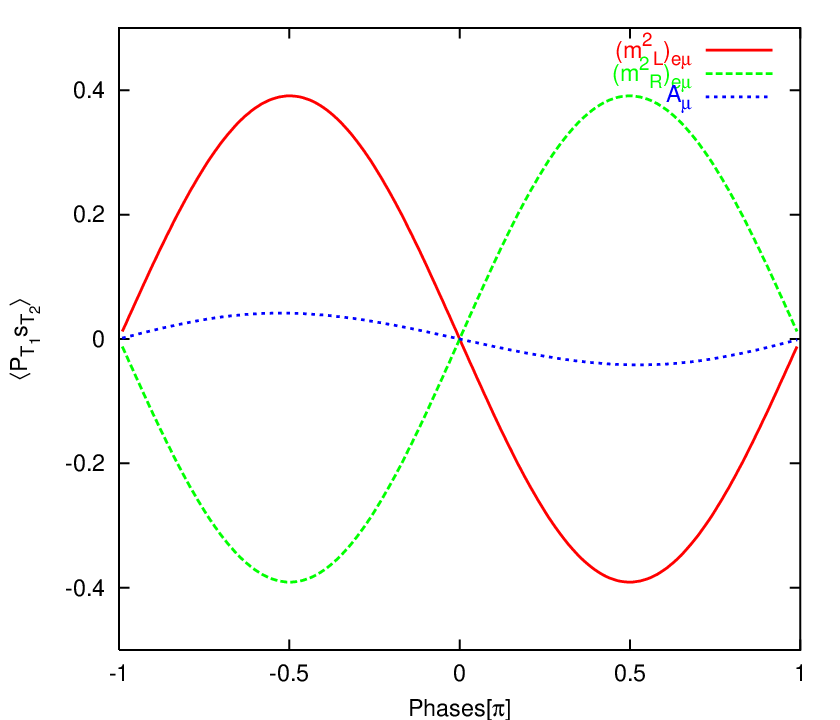
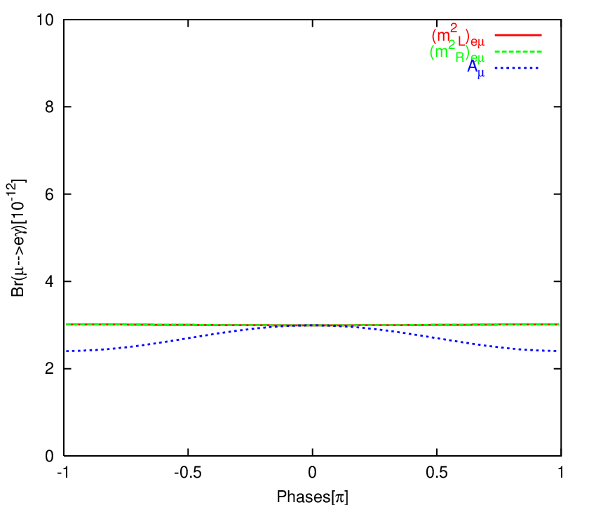
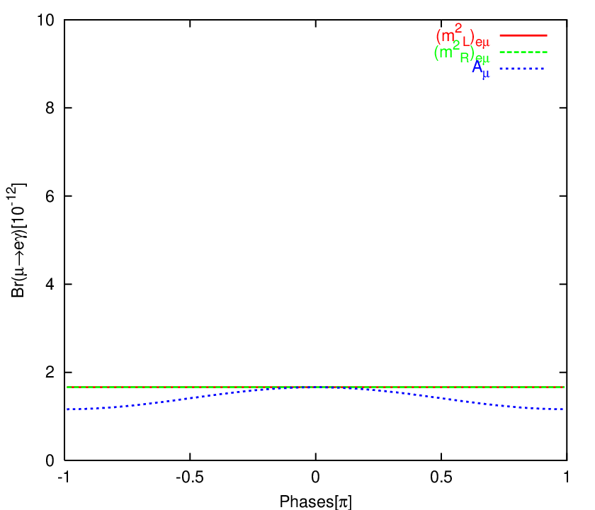
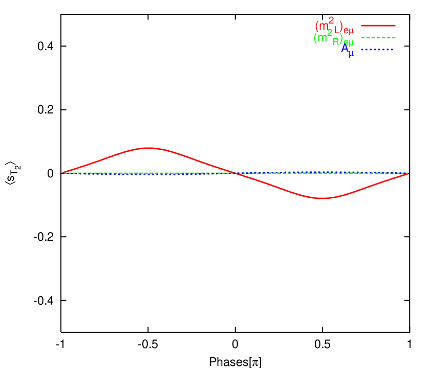
Figs. (1-3) shows , Br, and (see, Eqs. (4,10,11) for definitions) versus the phases of and the LFV elements. We have set however the results are robust against varying the values of as expected. In Fig. (1), we have taken and all the LFV elements of the slepton mass matrix other than and equal to zero. Notice that and have been chosen such that lies close to its present experimental upper bound. As seen from Fig. (1-c), for such choice of and , is close to zero which means . As a result, we expect the transverse polarization to be sizable. Figs. (1-a,1-b) demonstrate that this expectation is fulfilled. From Figs. (1-a,1-b), we also observe that the sensitivity of the transverse polarization to the phases of and is significant so by measuring these polarizations with a moderate accuracy one can extract information on these phases. However at this benchmark, the sensitivity to the phase of is quite low.
The input of Fig. (2) is similar to that of Fig. (1) except that a hierarchy is assumed between the left and right LFV elements: . As expected in this case, and the transverse polarizations are small. To draw Fig. (3), we have set the LFV elements of and equal to zero and instead we have set . As seen in Fig. (3) in this case, the transverse polarizations can be sizeable.
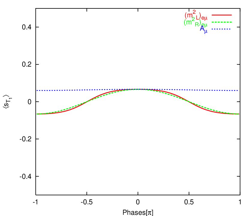
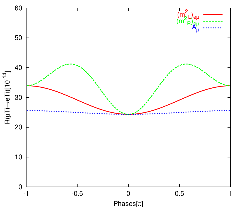
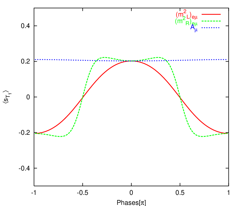
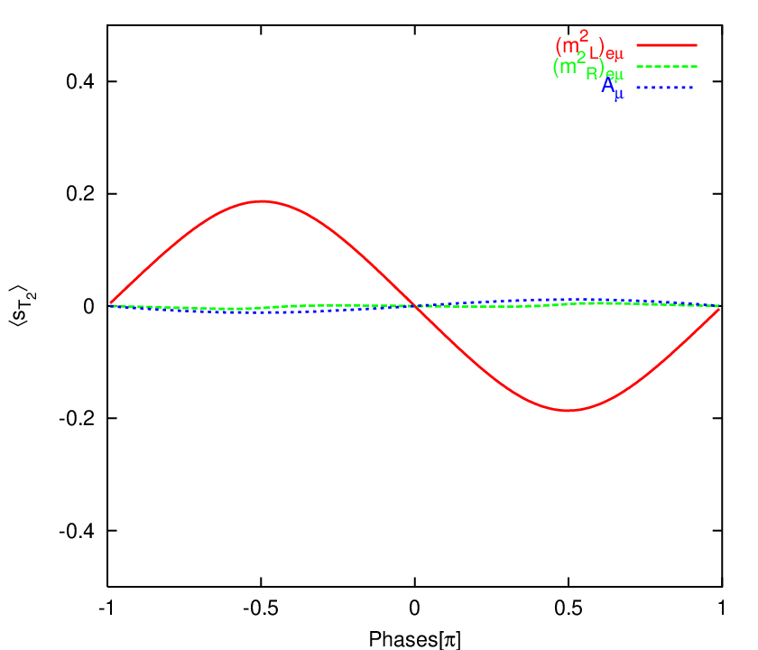
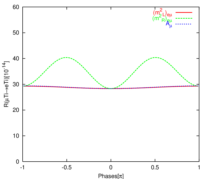
Figs. (4-6) show , , and (see, Eqs. (20,23,24) for definitions) versus the phases of and the LFV elements. To draw the figures corresponding to the conversion, we have taken . If the technical difficulties of polarizing the muon in the conversion experiment is overcome and higher values of is achieved, and can become larger. Obviously, for a given value of , and have to be re-scaled by . Apart from the polarization, the input parameters in Figs. (4,5,6) are respectively the same as the input parameters in Figs. (1,2,3). Notice that in this case, too, the sensitivity to the phase of is low. From Fig. (2), we observe that increases more rapidly with than with . For cases, at first sight, higher sensitivity to may sound counterintuitive. However, notice that as increases, rapidly converges to one which means and therefore
It is remarkable that in the case of Fig. (4) for which , is close to one and the transverse polarizations is relatively small but in the case of Fig. (5) for which , and the transverse polarizations become sizeable. We have explored higher hierarchy between the left and right LFV elements and have found that for , and diminish. Contrasting Figs. (4,5) with Figs. (1,2), we find that the polarization studies at the and conversion experiments can be complementary. That is if , transverse polarization in the will become small making the derivation of the CP-violating phases more challenging. However there is still the hope to derive the phases by polarization studies at the conversion experiments. We shall discuss this point in more detail in the description of Fig. 7.
Notice that in Figs. (1-6), which all correspond to the benchmark , sensitivity to the phase of is low. This is expected because the effect of is suppressed by . We have checked for the robustness of this result and found that for most of the parameter space with large , sensitivity to the phase of is low but there are points at which sensitivity to is considerable; e.g., at benchmark which has been proposed in [22].
The following remarks are in order:
- •
In all of these sets of diagrams, maximal corresponds to and vice versa. This is expected from Eqs. (23) and (24) because and are respectively given by the real and imaginary parts of the same combinations. For general values of the phases, is solely given by the absolute values of and , and is independent of their relative phase. Remember that and can be extracted by studying the angular distribution of the electron without measuring its spin. Thus, the simultaneous measurement of , and provides a cross-check. A similar consideration holds for , and , too.
- •
- •
When , in the case of , there is a symmetry under [see Figs. (1,2)] but in the case of the conversion, there is not such a symmetry [see Figs. (4,5)]. Moreover, while the dependence of on the phases is very mild, can dramatically change with varying some of the phases (see, e.g., Fig. (5-c)). This can be better understood in the limit of the LFV mass insertion approximation. Remember that observables in the decay are given by and for . To leading approximation, and are respectively proportional to and . As a result, when we vary the phase of , only the phase of changes. Similarly varying only changes . Since depends only on the absolute values of and , it should not change with varying the phases. Remember that and are given by and which to leading order are proportional to and . Thus, there should be a symmetry under for . Observables in the conversion case depend on and . Unlike and , each of and can receive contributions from both and . Thus, the above argument does not apply here. Similar consideration holds for the case that and are nonzero but (see, Figs. 3 and 6). As expected, when , , and are all nonzero, the symmetries under and disappear.
- •
In this analysis, we have considered the conversion only on Titanium. It is possible to perform the experiment on other nuclei such as Au and Al, too. From Eqs. (16,17), we find that the effects change with changing the nuclei (with change of and ). In principle, by studying the conversion rate on different nuclei, one can derive information on different combinations of the phases. However, in practice since the ratio for different nuclei in question are more or less the same (the difference between of Au and Al is about ), , and for different nuclei turn out to be close to each other. Only if can be measured with accuracy better than 5% (i.e., ), using different nuclei will help us to solve degeneracies.


(a) (b)


(c) (d)
Scatter plots shown in Fig. 7 demonstrate the configurations of the LFV elements where or can be sizeable. That is where maximal values of and are respectively larger than and . In Fig. (a) and (c) where only a pair of LFV are nonzero, only within a band and can be large. This is expected because when there is a hierarchy between the nonzero elements, we expect a hierarchy between and as well as between and thus and are suppressed. In Figs. (b) and (d), , , and are all nonzero. Notice that depending on the configuration of the LFV elements, the regions over which and are large can have partial (like Figs. a and d) or complete (like Figs. b and c). This confirms our observation regarding the previous figures. In the case of overlap, one can employ both experiments to derive information on the CP-violating phases. In the next section, we discuss how by combining the information from these two experiments, one can derive extra information and resolve degeneracies.
V Resolving Degeneracies
As discussed in the previous sections, all the observables in the experiment are determined by a pair of effective couplings () which in turn receive contributions from various parameters in the underlying theory. By measuring Br(), and either of and (see, Eqs. (10,11)), one can reconstruct both and (up to a common phase). However, because of the degeneracies, it is not possible to unambiguously derive the values of the LFV elements and the CP-violating phases of the underlying theory from and .
Similarly to the experiment, the observable quantities in the experiment are given by a pair of parameters () which depend on the LFV masses and CP-violating phases of the underlying theory. By measuring , and either of and (see, Eqs. (23,24)), it is possible to reconstruct , and their relative phase; however, deriving the LFV and CP-violating parameters of the underlying theory from would suffer from degeneracies.
(a) (b)
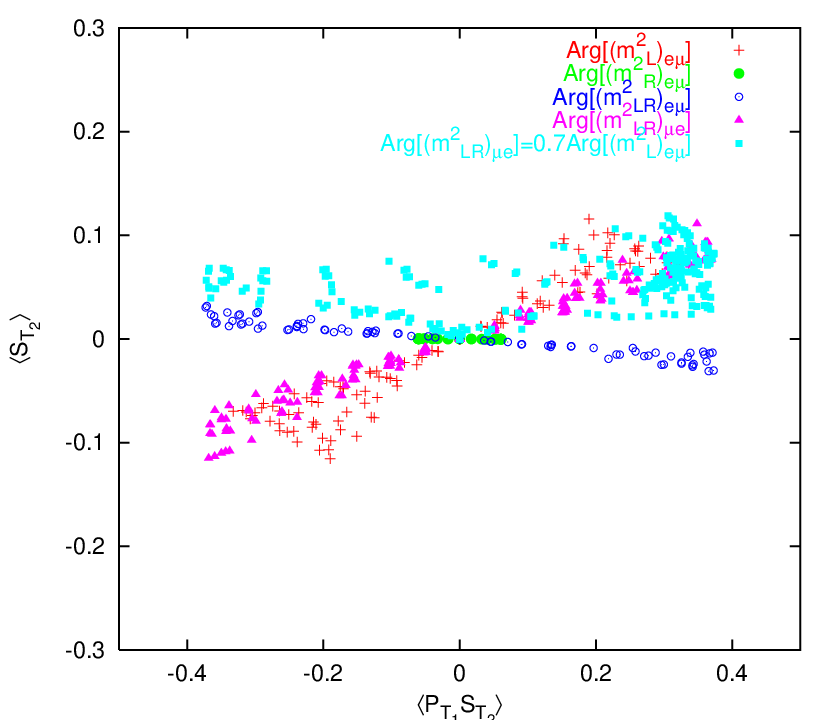
Fortunately, the pairs of () and depend on different combinations of the LFV elements. Thus, there is a hope to solve a part of degeneracies by combining information from the and experiments. Fig. 8 demonstrates such a possibility. In the case of the points depicted by red plus (+), green filled circle, dark blue circle and purple triangle, all the phases are set to zero except one of the phases which is specified in the legend and varies between 0 and . In the case of points depicted by cyan squares, the phase of is set equal to 0.7 of the phase of which varies between zero and (thus, varies between zero and ). The rest of the phases are set equal to zero. As we saw in the previous section, the sensitivity to the phase of is low (especially at the P3 benchmark) so in this analysis we have not considered this phase and focused on the effects of the phases of the LFV elements.
Hopefully, LHC will discover supersymmetry and provide us with information on the values of LF conserving parameters such as values of and the masses of neutralinos, charginos (hence the values of and ) and sfermions and etc. In the literature, it is discussed that under certain circumstances, LHC can also measure the LFV parameters [23]. However, in this analysis, we solely rely on the LFV rare processes and to derive the LFV parameters. Having this prospect in mind, we have chosen the values at the P3 benchmark for the lepton flavor conserving parameters. We have then searched for the values of the LFV elements at which the observable quantities Br, , and are in a given range. We have fixed and to 700 GeV. Notice that measuring and at LHC is going to be challenging if possible at all. In principle, we should have set and as free parameters to be determined from the and conversion experiments along with the LFV parameters. Notice however that, for , sensitivity to these parameters is low (i.e., varying from 0 to 700 GeV, the changes in the values of the observables are less than 5%). If turns out to be lower or a precision better than 5% is achieved, and should be treated as free parameters (rather than input).
The idea behind the plot is as follows. Suppose and are detected and their rates are measured with some reasonable accuracy. Moreover suppose and are measured and found to be in the range indicated in the caption of Fig. 8. The question is what configurations of LFV elements and the CP-violating phases can give rise to these values of the observables. To answer this question, we have looked for the solutions by varying , , and respectively in the range (, , ( and for given values of the CP-violating phases. We have then inserted the values of the LFV elements at the solutions in the formulas of and and depicted it in Fig. 8-a by a point.
From Fig. 8-a, we observe that all sets of the solutions depicted with various symbols reach to each other at the point . This is expected because setting the phases equal to zero renders , , and real so both and vanish (see, Eqs. (11,24)). Apart from this point, the set of points depicted by plus and triangles are separate from points depicted by empty circles which means by combining information from the and conversion searches, one can solve the degeneracy between these solutions. For example, if and , we can make sure that neither of the solutions with zero that we have considered in this analysis can be the case. However, the degeneracy is not completely solved. For example from Fig. 8-a, we observe that the regions over which points depicted by plus and square are scattered, overlap. At the intersection of the two regions, both () and () can be a solution.
We have repeated the same analysis for other ranges of , , Br() and . As long as and deviate from , the above results are maintained. However, when and approach , regardless of the values of the phases, the corresponding transverse polarizations become so small that in practice cannot be measured.
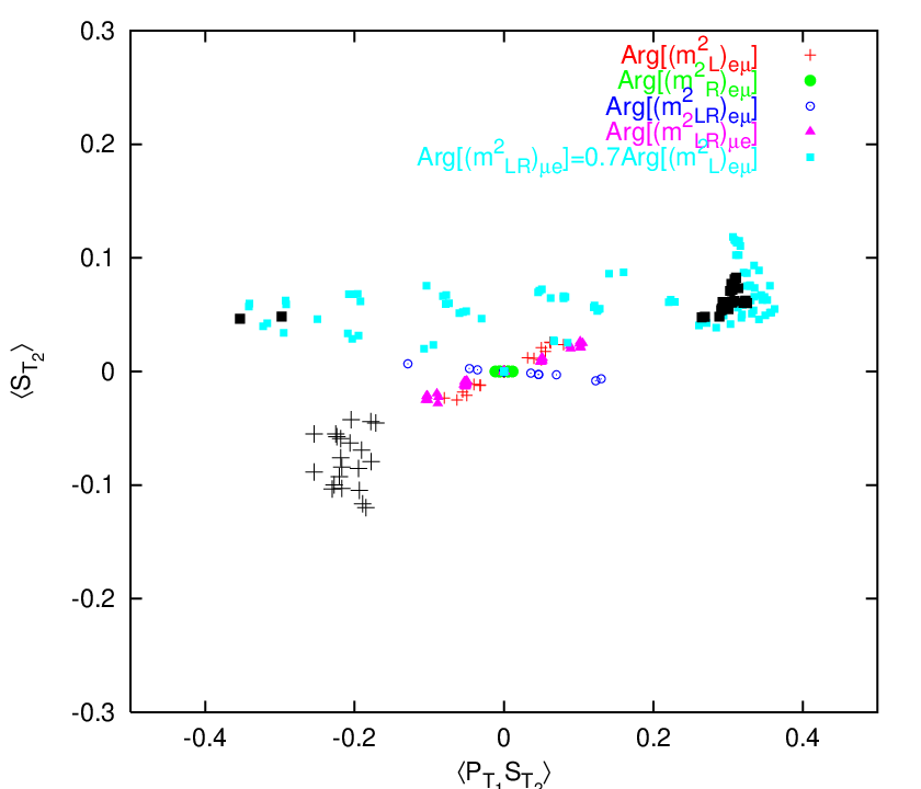
In summary, combining the information from and searches considerably lifts the degeneracies however, does not completely resolve them. By employing other observables, it may be possible to completely solve the degeneracies. For example, it is in principle possible to derive extra information on the elements by studying other LFV processes such as which within our scenario takes place with a rate suppressed by a factor of relative to the rate of . A more promising approach is to employ the information from the searches. As we discussed in the previous section, the phases of the elements can lead to cm which is within the reach of the currently running experiments [24]. To examine how much forthcoming results on can help us to resolve the degeneracies, we have presented Fig. (8-b). This figure is similar to Fig. (8-a) with the difference that at each point in addition to observables in the and conversion experiments, we have also calculated . We have removed the points for which cm from the set of points depicted by colored symbols. In the case of and , we have also depicted points satisfying the condition with slightly larger black symbols.
Notice that unlike in Fig. (a), in Fig. (b) the regions over which the squares and pluses are scattered have no overlap. This means can help us to resolve the degeneracies. For example according to Figs. (8-a,8-b), if and are measured and found to be respectively equal to 0.05 and 0.3, both and can be a solution. But if turns out to be in the range , the solution with will be excluded.
VI Conclusions
In this paper, we have first derived the formulas for the transverse polarization of the final particles in , and conversion in terms of the couplings of the effective LFV Lagrangian describing these processes. We have shown that by measuring these polarizations, one can derive information on the CP-violating phases of the underlying theory. We have then focused on the polarizations of the final particles in the and conversion processes. We have found that for the configurations of LFV elements that asymmetries and (see Eqs. (4,20) for definitions) are not close to , the transverse polarization can be sizeable and sensitive to certain combinations of the CP-violating phases. We therefore suggest the following steps as the strategy to extract the CP-violating phases. If in the future and/or conversion is detected with high statistics, it will be possible to measure and/or by studying the angular distribution of the final particles relative to the spin of the decaying muon. If and/or turn out to considerably deviate from , it is then recommendable to equip the experiment with polarimeters to measure the transverse polarizations of the final particles and derive information on the phases of the effective couplings.
The above results apply to a general beyond SM scenario that provides large enough sources of LFV to allow detectable rates for and . Within a given scenario, the couplings of the effective Lagrangian can depend on various parameters in the underlying theory. This leads to degeneracies in deriving these parameters. In this paper, we have addressed this problem in the context of -parity conserving MSSM. We have implicitly assumed that supersymmetry would be discovered at the LHC and the lepton flavor conserving parameters relevant for this study (e.g., chargino and neutralino masses, slepton and sfermion masses and etc.) would be measured. We have then studied what can be learnt about the LFV and CP-violating parameters of MSSM at and conversion experiments.
We have found that the dependence of the polarizations in the cases of and conversion on the parameters of the underlying theory is different. As a result, depending on the configuration of the LFV elements, the effect can be sizeable in none, only one or both of the and conversion processes. Thus, the polarization studies in these processes are complementary.
We have focused on the effect of the elements and studied the dependence of the various observables on the phases of and the LFV elements. Since there are already strong bounds on the phases of , (Bino mass) and from electric dipole moment searches, we have taken these parameters real. We have found that for most parts of the parameter space with large (i.e., ) the sensitivity to is low but the sensitivity of transverse polarizations both in and conversion to is high. However, there are regions in the parameter space that the sensitivity to is sizeable (e.g., the benchmark [22]). The sensitivity to in the case of is also high but in the case of the conversion, the sensitivity to is low.
In the context of the present scenario, various CP-violating parameters can affect the observables in the and experiments. These polarizations also strongly depend on the ratios of the absolute values of the various LFV elements. We have shown that for configurations of LFV elements for which , combining information on , , Br and with information on the transverse polarization of the final particles can help us to considerably decrease degeneracies and derive information on these phases. However, information from these measurements is not enough to fully resolve degeneracies. For example, we have shown degeneracies between solutions and cannot be removed even when we use all the information accessible at the and search experiments. To fully resolve the degeneracies, extra information from other experiments has to be employed. We have also demonstrated that the forthcoming results of the search can help us to remove the degeneracies further.
Notice that by [simultaneously] turning on the and elements, more degeneracies will emerge. To resolve these degeneracies, one can employ other observables such as Br() and Br(). Studying the general case is beyond the scope of the present paper and will be presented elsewhere.
We have also briefly discussed the possibility to derive further information by using different nuclei in the conversion experiment and found that since the ratio of proton number to the neutron number for different nuclei is close to each other, the polarizations are similar for different nuclei. Unless a precision better than 5% is achieved, changing the nuclei will not help us to extract information on an extra combination of the parameters but can be considered as a cross-check of the results.
Acknowledgement
We would like to thank M. M. Sheikh-Jabbari for careful reading of the manuscript and the useful remarks.
References
- [1] S. T. Petcov, Sov. J. Nucl. Phys. 25 (1977) 340 [Yad. Fiz. 25 (1977 ERRAT,25,698.1977 ERRAT,25,1336.1977) 641]; S. M. Bilenky, S. T. Petcov and B. Pontecorvo, Phys. Lett. B 67 (1977) 309; G. Altarelli, L. Baulieu, N. Cabibbo, L. Maiani and R. Petronzio, Nucl. Phys. B 125 (1977) 285 [Erratum-ibid. B 130 (1977) 516].
- [2] W. M. Yao et al. [Particle Data Group], J. Phys. G 33 (2006) 1.
- [3] http://meg.web.psi.ch/index.html; see also M. Grassi [MEG Collaboration], Nucl. Phys. Proc. Suppl. 149 (2005) 369.
- [4] Y. Kuno and Y. Okada, Rev. Mod. Phys. 73, 151 (2001) [arXiv:hep-ph/9909265]; J. L. Feng, arXiv:hep-ph/0101122.
- [5] Y. Farzan, JHEP 0707 (2007) 054 [arXiv:hep-ph/0701106].
- [6] R. M. Godbole, Czech. J. Phys. 55 (2005) B221 [arXiv:hep-ph/0503088]; O. Kittel, arXiv:hep-ph/0504183; S. Heinemeyer and M. Velasco, In the Proceedings of 2005 International Linear Collider Workshop (LCWS 2005), Stanford, California, 18-22 Mar 2005, pp 0508 [arXiv:hep-ph/0506267].
- [7] A. van der Schaaf, J. Phys. G 29 (2003) 1503; W. Bertl et al. [SINDRUM II Collaboration], Eur. Phys. J. C 47 (2006) 337;
- [8] P. Wintz, in Proceedings of the First International Symposium on Lepton and Baryon number Violation, edited by H. V. Kalpdor-Kleingrothaus and I. V. Krivosheina (Institute of Physics Publishing, Bristol and Philadelphia), p. 534.
- [9] M. Aoki, Prepared for Joint U.S. / Japan Workshop on New Initiatives in Muon Lepton Flavor Violation and Neutrino Oscillation with High Intense Muon and Neutrino Sources, Honolulu, Hawaii, 2-6 Oct 2000; Y. Mori, Prepared for 7th European Particle Accelerator Conference (EPAC 2000), Vienna, Austria, 26-30 Jun 2000;Y. Kuno, Nucl. Phys. Proc. Suppl. 149 (2005) 376; see also, E. J. Prebys et al., “Expression Of Interest: A Muon To Electron Conversion Experiment At Fermilab.”
- [10] S. Davidson, arXiv:0809.0263 [hep-ph].
- [11] J. Hisano, T. Moroi, K. Tobe and M. Yamaguchi, Phys. Rev. D 53 (1996) 2442 [arXiv:hep-ph/9510309].
- [12] Y. Okada, K. i. Okumura and Y. Shimizu, Phys. Rev. D 61 (2000) 094001 [arXiv:hep-ph/9906446].
- [13] H. Burkard et al., Phys. Lett. B 160 (1985) 343.
- [14] P. F. Bloser, S. D. Hunter, G. O. Depaola and F. Longo, arXiv:astro-ph/0308331; F. Adamyan et. al, Nucl. Ins. and Meth. in Phys. Research A 546 (2005) 376.
- [15] V. S. Evseev, in Muon Physics Vol. III Chemistry and Solids, 1975, edited by V. W. Hughes and C. S. Wu (Academic Press), p. 236.
- [16] K. Nagamine and T. Yamazaki, Nucl. Phys. A 219 (1974) 104; Y. Kuno, K. Nagamine and T. Yamazaki, Nucl. Phys. A 475 (1987) 615.
- [17] S. Yaser Ayazi and Y. Farzan, Phys. Rev. D 74 (2006) 055008 [arXiv:hep-ph/0605272] and references therein.
- [18] S. Y. Ayazi and Y. Farzan, JHEP 0706, 013 (2007) [arXiv:hep-ph/0702149].
- [19] A. Bartl, W. Majerotto, W. Porod and D. Wyler, Phys. Rev. D 68 (2003) 053005 [arXiv:hep-ph/0306050]; W. Porod, Prepared for International Workshop on Astroparticle and High-Energy Physics (AHEP-2003), Valencia, Spain, 14-18 Oct 2003.
- [20] J. Ellis, T. Hahn, S. Heinemeyer, K. A. Olive and G. Weiglein, JHEP 0710, 092 (2007) [arXiv:0709.0098 [hep-ph]]; S. Heinemeyer, arXiv:0710.3014 [hep-ph].
- [21] J. A. Casas and S. Dimopoulos, Phys. Lett. B 387, 107 (1996) [arXiv:hep-ph/9606237].
- [22] A. De Roeck, J. R. Ellis, F. Gianotti, F. Moortgat, K. A. Olive and L. Pape, Eur. Phys. J. C 49 (2007) 1041 [arXiv:hep-ph/0508198].
- [23] J. L. Diaz-Cruz, D. K. Ghosh and S. Moretti, arXiv:0809.5158 [hep-ph].
- [24] D. DeMille, S. Bickman, P. Hamilton, Y. Jiang, V. Prasad, D. Kawall and R. Paolino, AIP Conf. Proc. 842 (2006) 759.