Introduction

AMS 57M25

ISSN 0239-8885

UNIWERSYTET WARSZAWSKI

INSTYTUT MATEMATYKI

Józef H. Przytycki

Survey on recent invariants on classical knot theory

I. Conway Algebras

Preprint 6/86

“na prawach rȩkopisu”

Warszawa 1986

Introduction

The purpose of this survey is to present a new combinatorial method of constructing invariants of isotopy classes of tame links. The period of time between the spring of 1984 and the summer of 1985 was full of discoveries which revolutionized the knot theory and will have a deep impact on some other branches of mathematics. It started by the discovery of Jones of the new polynomial invariant of links (in May 1984; [Jo–1], [Jo–2]) and the last big step (which will be described in this survey) has been made by Kauffman [K–5] in August 1985 when Kauffman applied his method which allowed him to unify almost all previous work. This survey is far from being complete, even if we limit ourselves to the purely combinatorial methods and to the period May, 1984 – September, 1985. (Since then, new important results have been obtained.) In particular, we don’t include the very interesting results of Lickorish and Millett [Li–M–2], results which link some substitutions in the Jones-Conway polynomial with old invariants of links.

The survey consists of five parts:

(1)

Diagrams of links and Reidemeister moves.

This chapter makes the survey almost self-contained and makes it accessible to non-specialists.
(2)

Conway algebras and their invariants of links.

We consider in this chapter invariants of oriented links which have the following striking common feature: If $L_{+}$ , $L_{-}$ , and $L_{\circ}$ are diagrams of oriented links which are identical, except near one crossing point where they are as in Figure 0.1, then the value of the invariant for $L_{+}$ is uniquely determined by the values of the invariant for $L_{-}$ and $L_{\circ}$ , and the value of the invariant for $L_{-}$ is uniquely determined by the values of the invariant for $L_{+}$ and $L_{\circ}$ .

Figure 0.1.

We construct an abstract algebra (called the Conway algebra) which formalizes the above approach.
(3)

Skein equivalence and properties of the invariants of Conway type.

We consider the properties of the invariants under reflection, mutation, connected and disjoint sums of links. We analyze closer the Jones-Conway (HOMFLY) polynomial.
(4)

Partial Conway algebras.

The generalization of Conway algebras, described in this chapter, allows for the construction of new invariants of links; in particular, a polynomial of infinitely many variables and a supersignature.
(5)

Kauffman approach.

The additional diagram $L_{\infty}$ (Figure 0.2) allows the construction of a new link invariant ([B–L–M] and [Ho]).

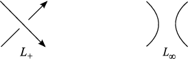
Figure 0.2.

Kauffman uses regular isotopy of diagrams of links (instead of isotopy) to build a polynomial invariant of links which generalizes the previously known one. We construct an algebraic structure (Kauffman algebra) which allows us to describe invariants obtained via the Kauffman method in a unified way.

This survey is a detailed presentation of the eight lectures given by the author at the University of Zaragoza in February of 1986. The author would like to thank José Montesinos for his exceptional hospitality.

1. Link diagrams and Reidemeister moves

The classical knot theory studies the position of a circle (knots) or of several circles (links) in $S^{3}$ (or $\mathbb{R}^{3}$ ). We say that two links $L_{1}$ and $L_{2}$ in $S^{3}$ are isotopic, written $L_{1}\approx L_{2}$ , if there exists an isotopy $F:S^{3}\times I\longrightarrow S^{3}\times I$ such that $F_{0}=\mathrm{Id}$ and $F_{1}(L_{1})=L_{2}$ . If the links $L_{1}$ and $L_{2}$ are oriented, we assume additionally that $F_{1}$ preserves orientations of the links.

We work all the time in the PL category; smooth category could be considered equally well. $S^{3}=\mathbb{R}^{3}\cup\infty$ and we can always assume that the link omits $\infty$ . It is not difficult to show that two links are isotopic in $\mathbb{R}^{3}$ if and only if they are isotopic in $S^{3}$ . Links (up to isotopy) can be represented by their diagrams on the plane. Namely, let $p:\mathbb{R}^{3}\longrightarrow\mathbb{R}^{2}$ be a projection and $L\subset\mathbb{R}^{3}$ a link. A point $P\in p(L)\subset\mathbb{R}^{2}$ whose preimage, $p^{-1}(P)$ , contains more than one point is called a multiple point. A projection $p$ is called regular if

(1)

There are only finitely many multiple points, and all multiple points are double points (called crossings), and
(2)

$P/L:L\to\mathbb{R}^{2}$ is the general position projection (in some triangulation of $(\mathbb{R}^{3},L)$ and $\mathbb{R}^{2}$ , in which $P/L$ is simplicial, no double points of $L$ are vertices).

If, for a given regular projection of a link, all over-crossings (bridges) at every crossing are marked, then the link can be reconstructed from the projection. The projection of the link with just described additional information is called the diagram of the link.

We call two diagrams equivalent (in oriented or unoriented category) if they describe isotopic links. The following theorem of Reidemeister allows us to work entirely with diagrams.

Theorem 1.0.1.

Two link diagrams are equivalent if and only if they are connected by a finite sequence of Reidemeister moves, $\Omega^{\pm 1}_{i}$ $(i=1,2,3)$ see Figure 1.1.

2. Conway algebras and their invariants of links

2.1. Conway algebras

¹¹ 1 The equation numbers in this subsection are off by one from the original.

Conway [Co], considering the quick methods of computing the Alexander polynomial of links, suggested a special normed form of it (which we call the Conway polynomial) and he showed that the Conway polynomial, $\nabla_{L}(z)$ , satisfies

(1)

$\nabla_{T_{1}}(z)=1$ , where $T_{1}$ is the trivial knot
(2)

$\nabla_{L_{+}}(z)-\nabla_{L_{-}}(z)=z\nabla_{L_{\circ}}(z)$ , where $L_{+}$ , $L_{-}$ , and $L_{\circ}$ are diagrams of oriented links which are identical, except near one crossing point, where they look like in Figure 2.1.1²² 2 The remaining figures in this section have their number shifted by one from the original, where there were two Figures 2.1.1..

Furthermore, conditions (1) and (2) define uniquely $\nabla_{L}(z)$ ; [Co], [K–2], [Gi], [B–M].

At spring of 1984, V. Jones [Jo–1], [Jo–2]has shown that there exists an invariant of oriented links which is a Laurent polynomial of $\sqrt{t}$ and which satisfies:

(1)

$V_{T_{1}}(t)=1$ , and
(2)

$-tV_{L_{+}}+\frac{1}{t}V_{L_{-}}=\left(\sqrt{t}-\frac{1}{\sqrt{t}}\right)V_{L_{\circ}}(t).$

It was an immediate idea, after these two examples, that there exists an invariant of isotopy of oriented links which is a Laurent polynomial of 2-variables $(P_{L}(x,y))$ which satisfies:

(1)

$P_{T_{1}}(x,y)=1$ , and
(2)

$xP_{L_{+}}(x,y)+yP_{L_{-}}(x,y)=P_{L_{\circ}}(x,y)$ .

In fact, such an invariant exists and it was discovered four months after the Jones polynomial (in September of 1984) by four groups of researchers: R. Lickorish and K. Millett, J. Hoste, A. Ocneanu, P. Freyd, and D. Yetter [F–Y–H–L–M–O] (and independently in early December of 1984 by J. Przytycki and P. Traczyk [P–T–1]). We will call this polynomial the Jones-Conway polynomial or HOMFLY polynomial (after initials of the inventors of it).

Instead of looking for polynomial invariants of links related to Figure 2.1.1, we can consider a more general point of view. Namely, we can look for general invariants of links which have the following common feature: $w_{L_{+}}$ is uniquely determined by $w_{L_{-}}$ and $w_{L_{\circ}}$ , and also $w_{L_{-}}$ is uniquely determined by $w_{L_{+}}$ and $w_{L_{\circ}}$ . Invariants with this property we call Conway type invariants. Now we will develop this idea based mainly on the paper [P–T–1].

Consider the following general situation. Assume we are given a set $A$ (called universum) with a sequence of fixed elements, $a_{1},a_{2},\ldots$ (i.e. a function $f:\mathbb{N}\to A$ ) and two $2$ -argument operations, $|$ and $\ast$ , each mapping $A\times A$ into $A$ . (That is, we have an algebra $\mathcal{A}=(A;a_{1},a_{2},\ldots,|,\ast)$ .) We would like to construct invariants of oriented links satisfying the conditions:

\begin{array}[]{l}w_{L_{+}}=w_{L_{-}}|w_{L_{\circ}}\textrm{,}\\ w_{L_{-}}=w_{L_{+}}\ast w_{L_{\circ}}\textrm{, and}\\ w_{T_{n}}=a_{n}\textrm{, where }T_{n}\textrm{ is the trivial link with }n\textrm{ components.}\end{array}

Definition 2.1.1.

We say that $\mathcal{A}=(A;a_{1},a_{2},\ldots,|,\ast)$ is a Conway algebra if the following conditions are satisfied:

C1.

$a_{n}|a_{n+1}=a_{n}$
C2.

$a_{n}\ast a_{n+1}=a_{n}$
C3.

$(a|b)|(c|d)=(a|c)|(b|d)$
C4.

$(a|b)\ast(c|d)=(a\ast c)|(b\ast d)$
C5.

$(a\ast b)\ast(c\ast d)=(a\ast c)\ast(b\ast d)$
C6.

$(a|b)\ast b=a$
C7.

$(a\ast b)|b=a$

Note that C3 through C5 are transposition properties.

The following is the main theorem of [P–T–1].

Theorem 2.1.2.

³³ 3 In the original, this Theorem was mistakenly numbered 2.1.1, but referenced as 2.1.2 throughout.

For a given Conway algebra $\mathcal{A}$ , there exists a uniquely determined invariant, $w$ , which attaches an element $w_{L}$ from $A$ to every isotopy class of oriented links and satisfies the conditions

(1)

$\begin{array}[]{l}w_{T_{n}}=a_{n}\end{array}\textrm{(initial conditions)}$
(2)

$\begin{array}[]{l}w_{L_{+}}=w_{L_{-}}|w_{L_{\circ}}\\ w_{L_{-}}=w_{L_{+}}\ast w_{L_{\circ}}\end{array}\textrm{(Conway relations)}$

Before we give the proof, let us write here a few words about the geometrical meaning of the axioms C1–C7 of Conway algebra. Relations C1 and C2 are introduced to reflect the following geometrical relations between the diagrams of trivial links of $n$ and $n+1$ components:

Relations C3–C5 arise when considering rearranging a link at two crossings of the diagram, but in different order. It will be explained in the proof of Theorem 2.1.2. Relations C6 and C7 reflect the fact that we need the operations $|$ and $\ast$ to be in some respects opposite to one another.

Before giving examples (models) of Conway algebra and sketching the proof of Theorem 2.1.2, we will show some elementary properties of Conway algebra. We have introduced in the definition seven conditions mainly because of esthetic and practical reasons (the roles of operations $|$ and $\ast$ are equivalent). These conditions, however, often depend on one another:

Lemma 2.1.3.

We have the following dependencies among axioms C1–C7:

(a)

C1 and C6 $\Rightarrow$ C2
(b)

C2 and C7 $\Rightarrow$ C1
(c)

C6 and C4 $\Rightarrow$ C7
(d)

C7 and C4 $\Rightarrow$ C6
(e)

C6 and C4 $\Rightarrow$ C5
(f)

C7 and C4 $\Rightarrow$ C3
(g)

C5, C6 and C7 $\Rightarrow$ C4
(h)

C3, C6, and C7 $\Rightarrow$ C4

Proof.

We will prove, as examples, (a), (c), (e), and (g).

(a)

$\textrm{C1}\iff a_{n}|a_{n+1}=a_{n}\implies(a_{n}|a_{n+1})\ast a_{n+1}=a_{n}\ast a_{n+1}\overset{\textrm{C6}}{\implies}\newline \overset{\textrm{C6}}{\implies}a_{n}=a_{n}\ast a_{n+1}\iff\textrm{C2}$ .
(c)

$\textrm{C6}\implies(a|(b|a))\ast(b|a)=a\overset{\textrm{C4}}{\iff}(a\ast b)|((b|a)\ast a)=a\overset{\textrm{1.6}}{\implies}\newline \overset{\textrm{1.6}}{\implies}(a\ast b)|b=a\iff\textrm{C7}$ .

(e), (g)

\begin{array}[]{lcccc}\textrm{C5}&\iff&(a\ast b)\ast(c\ast d)&=&(a\ast c)\ast(b\ast d)\\ &&\Downarrow\textrm{C7}&&\textrm{C6}\Uparrow\\ &&(a\ast b)&=&((a\ast c)\ast(b\ast d))|(c\ast d)\\ &&&\Updownarrow\textrm{C7}&\textrm{(or C6 and C4 by (c))}\\ \textrm{C4}&\implies&((a\ast c)|c)\ast((b\ast d)|d)&=&((a\ast c)\ast(b\ast d))|(c\ast d)\\ &&\textrm{substitute }a=x|c\textrm{ and }b=y|d&\Downarrow\textrm{C6}&\\ &&(x|c)\ast(y|d)&=&(x\ast y)|(c\ast d)\\ &&&\Updownarrow\\ &&&\textrm{C4}\end{array}

∎

Lemma 2.1.4.

Let us define in each Conway algebra $\mathcal{A}$ and for each $b\in A$ and action $|_{b}$ (respectively, $\ast_{b}$ ) $:A\to A$ defined by $|_{b}(a)=a|b$ (respectively, $\ast_{b}(a)=a\ast b$ ). Then $|_{b}$ and $\ast_{b}$ are bijections on $A$ . Furthermore, $|_{b}$ and $\ast_{b}$ are inverses one to another, i.e. $|_{b}\ast_{b}=\ast_{b}|_{b}=\mathrm{Id}$ .

Lemma 2.1.4 follows from conditions C6 and C7. Now we will describe some examples of Conway algebras.

Example 2.1.5 (Number of components).

Set $A=\mathbb{N}$ (the set of natural numbers), $a_{i}=i$ , and $i|j=i\ast j=i$ . Verification of conditions C1–C7 is immediate (the first letter of each side of every relation is the same). This algebra yields the number of components of the link.

Example 2.1.6.

Set $A=\{0,1,2\}$ , $a_{i}\equiv i\mod 3$ , the operation $\ast$ is equal to $|$ , and $|$ is given by the following table:

$\|$	0	1	2
0	1	0	2
1	0	2	1
2	2	1	0

The invariant defined by this algebra distinguishes, for example, the trefoil knot from the trivial knot (Figure 2.1.3).

Example 2.1.7.

Set $A=\{1,2,3,4\}$ , $a_{1}=1$ , $a_{2}=2$ , $a_{3}=4$ , $a_{4}=1$ , $a_{5}=2$ , $a_{6}=4$ , $\ldots$ . Operations $|$ and $\ast$ are given by the following tables:

\begin{array}[]{lll}\begin{tabular}[]{c|cccc}$|$&1&2&3&4\\ \hline\cr 1&2&1&4&3\\ 2&3&4&1&2\\ 3&1&2&3&4\\ 4&4&3&2&1\end{tabular}&&\begin{tabular}[]{c|cccc}$\ast$&1&2&3&4\\ \hline\cr 1&3&1&2&4\\ 2&1&3&4&2\\ 3&2&4&3&1\\ 4&4&2&1&3\end{tabular}\end{array}

	$\begin{array}[]{lll}\begin{tabular}[]{c\|cccc}$\|$&1&2&3&4\\ \hline\cr 1&2&1&4&3\\ 2&3&4&1&2\\ 3&1&2&3&4\\ 4&4&3&2&1\end{tabular}&&\begin{tabular}[]{c\|cccc}$\ast$&1&2&3&4\\ \hline\cr 1&3&1&2&4\\ 2&1&3&4&2\\ 3&2&4&3&1\\ 4&4&2&1&3\end{tabular}\end{array}$	$\|$	1	2	3	4	$\ast$	1	2	3	4

The invariant defined by this algebra distinguishes the right-handed trefoil knot from the left-handed trefoil (Figure 2.1.4).

T. Przytycka has found (using a computer) all Conway algebras with no more than five elements. If we limit fixed elements to $a_{1}$ and $a_{2}$ and assume $a_{1}=1$ , $a_{2}=2$ then we get (up to isomorphism):

Number of elements	Number of algebras
2	2
3	9
4	51
5	204

Example 2.1.8 (Jones-Conway polynomial).

$A=\mathbb{Z}[x^{\mp},y^{\mp}]$ , $a_{1}=1,a_{2}=x+y,\ldots,a_{i}=(x+y)^{i-1},\ldots$ .

We define $|$ and $\ast$ as follows: $w_{2}|w_{0}=w_{1}$ and $w_{1}\ast w_{0}=w_{2}$ , where polynomials $w_{1}$ , $w_{2}$ , and $w_{0}$ satisfy the following equation:

(2.1.1)

xw_{1}+yw_{2}=w_{0}

The invariant of knots given by this algebra is the Jones-Conway polynomial mentioned at the beginning of this part. In particular, if we substitute $x=\frac{1}{z}$ and $y=-\frac{1}{z}$ we get the Conway polynomial, and after the substitution $x=\frac{-t}{\sqrt{t}-\frac{1}{\sqrt{t}}}$ , $y=\frac{1}{t}\frac{1}{\sqrt{t}-\frac{1}{\sqrt{t}}}$ , we get the Jones polynomial.

Now we will show that the algebra from Example 2.1.8 is in fact a Conway algebra.

The conditions C1 and C2 follow from the equality

x(x+y)^{n-1}+y(x+y)^{n-1}=(x+y)^{n}.

The conditions C6 and C7 follow from the fact that the actions were defined using one linear equation. It remains to show C3 (C4 and C5 will follow then by Lemma 2.1.3). We have from the definition

(a|b)|(c|d)=\frac{1}{x}((c|d)-y(a|b))=\frac{1}{x}\left(\frac{1}{x}(d-yc)-y\frac{1}{x}(b-ya)\right)=\frac{1}{x^{2}}d-\frac{y}{x^{2}}c-\frac{y}{x^{2}}b+\frac{y^{2}}{x^{2}}a.

Because coefficients of $b$ and $c$ are the same, if we change the places of $b$ and $c$ , the value of the expression is not changed, which proves condition C3.

It is possible to generalize the algebra of Example 2.1.8 by introducing the new variable $z$ and considering instead of 2.1.1, the equation

xw_{1}+yw_{2}=w_{0}-z.

However, one does not get any stronger invariant than the Jones-Conway polynomial (see Proposition 3.38).

Example 2.1.10 (Global linking number).

Set $A=\mathbb{N}\times\mathbb{Z}$ , $a_{i}=(i,0)$ , and

\begin{array}[]{l}(a,b)|(c,d)=\left\{\begin{array}[]{ll}(a,b+1)&\textrm{if }a>c\\ (a,b)&\textrm{if }a\leq c\end{array}\right.\\ (a,b)\ast(c,d)=\left\{\begin{array}[]{ll}(a,b-1)&\textrm{if }a>c\\ (a,b)&\textrm{if }a\leq c\end{array}\right.\end{array}

The invariant associated to a link is a pair: (number of components, global linking number).

It is an easy exercise to read the global linking number from the diagram. Namely, call a crossing of type positive and a crossing of type negative. We will write $\mathrm{sgn~}p=+$ or $-$ depending on whether the crossing $p$ is positive or negative. Then for a given diagram $D$ , $\mathrm{lk}(D)=\frac{1}{2}\sum\mathrm{sgn~}p_{i}$ , where summation is taken over all crossings between different components of $D$ , is equal to the global index number of $D$ .

Now we will show that the algebra from Example 2.1.10 is in fact a Conway algebra. The proof of conditions C1, C2, C6, and C7 is very easy and we omit it. We consider condition C3 in more detail. From the definition of the operation $|$ we have

((a_{1},a_{2})|(b_{1},b_{2}))|((c_{1},c_{2})|(d_{1},d_{2}))=\left\{\begin{array}[]{ll}(a_{1},a_{2}+2)&\textrm{if }a_{1}>b_{1}\textrm{ and }a_{1}>c_{1}\\ (a_{1},a_{2}+1)&\textrm{if }(a_{1}>b_{1}\textrm{ and }a_{1}\leq c_{1})\\ &\textrm{ or }(a_{1}\leq b_{1}\textrm{ and }a_{1}>c_{1})\\ (a_{1},a_{2})&\textrm{if }a_{1}\leq b_{1},a_{1}\leq c_{1}\end{array}\right.

If we exchange the places of $b_{i}$ and $c_{i}$ then we get the same result, so C3 is satisfied.

We will write $L^{p}_{+}$ , $L^{p}_{-}$ , and $L^{p}_{\circ}$ if we need the crossing point $p$ to be explicitly specified.

Definition 2.1.11.

Let $T$ be a binary tree each of whose vertices represents a link (trivial links at leaves) in such a way that the situation at each vertex (except at leaves) looks like:

Figure 2.1.5.

In a natural way it yields a binary tree with $a_{i}$ ’s at leaves and $+$ ’s or $-$ ’s at other vertices. We will call it a resolving tree of the root link.

Example 2.1.12.

Let $L$ be the figure-eight knot represented by the diagram in Figure 2.1.6.

To determine $w_{L}$ , let us consider the binary tree in Figure 2.1.7.

As is easily seen, the leaves of the tree are trivial links and every branching reflects a certain operation on the diagram at the marked crossing point. To compute $w_{L}$ , it is enough to have the resolving tree shown in Figure 2.1.8.

Here the sign indicates the sign of the crossing point at which the operation was performed, and the leaf entries are the values of $w$ for the resulting trivial links. Now we may conclude that $w_{L}=a_{1}|(a_{2}\ast a_{1})$ .

Figure 2.1.8.

There exists a standard procedure to obtain a resolving tree of a given diagram. It will be described in the next paragraph and it will play an essential role in the proof of Theorem 2.1.2.

2.2. Proof of Theorem 2.1.2

Definition 2.2.1.

Let $L$ be an oriented diagram of $n$ components and let $b=(b_{1},\ldots,b_{n})$ be base points of $L$ , one point from each component of $L$ , but not the crossing points. Then we say that $L$ is descending with respect to $b$ if the following holds: If one travels along $L$ (according to the orientation of $L$ ) starting from $b_{1}$ , then after having returned to $b_{1}$ – from $b_{2},\ldots,$ finally from $b_{n}$ , then each crossing which is met for the first time is crossed by an over-crossing (bridge).

It is easily seen that for every diagram $L$ of an oriented link there exists a resolving tree such that the leaf diagrams are descending (with respect to appropriately chosen base points). This is obvious for diagrams with no crossings at all, and once it is known for diagrams with less than $n$ crossings we can use the following procedure for any diagram with $n$ crossings: Choose base points arbitrarily and start walking along the diagram until the first “bad” crossing $p$ is met, i.e. the first crossing which is crossed by an under-crossing (tunnel) when first met. Then begin to construct the tree changing the diagram in this point. If for example $\mathrm{sgn~}p=+$ , we get

Then we can apply the inductive hypothesis to $L^{p}_{\circ}$ and we can continue the procedure with $L^{p}_{-}$ (walking further along the diagram and looking for the next bad point).

To prove Theorem 2.1.2, we will construct the function $w$ as defined on diagrams. In order to show that $w$ is an invariant of isotopy classes of oriented links we will verify that $w$ is preserved by the Reidemeister moves.

We use induction on the number $\mathrm{cr}(L)$ of crossing points in the diagram. For each $k\geq 0$ we define a function $w_{k}$ assigning an element of $A$ to each diagram of an oriented link with no more than $k$ crossings. Then $w$ will be defined for every diagram by $w_{L}=w_{k}(L)$ where $k\geq\mathrm{cr}(L)$ . Of course the function $w_{k}$ must satisfy certain coherence conditions for this to work. Finally, we will obtain the required properties of $w$ from the properties of the $w_{k}$ ’s.

We begin from the definition of $w_{0}$ . For a diagram $L$ of $n$ components with $\mathrm{cr}(L)=0$ , we put

(2.2.2)

w_{0}(L)=a_{n}.

To define $w_{k+1}$ and prove its properties we will use the induction several times. To avoid misunderstandings, the following will be called the Main Inductive Hypothesis (M.I.H.): We assume that we have already defined a function $w_{k}$ attaching an element of $A$ to each diagram $L$ for which $\mathrm{cr}(L)\leq k$ . We assume that $w_{k}$ has the following properties:

(2.2.3)

w_{k}(U_{n})=a_{n}

for $U_{n}$ being a descending diagram of $n$ components (with respect to some choice of base points).

(2.2.4)		$\displaystyle w_{k}(L_{+})=w_{k}(L_{-})\|w_{k}(L_{\circ})$
(2.2.5)		$\displaystyle w_{k}(L_{-})=w_{k}(L_{+})\ast w_{k}(L_{\circ}),$

for $L_{+}$ , $L_{-}$ , and $L_{\circ}$ related as usually, and

(2.2.6)

w_{k}(L)=w_{k}(R(L)),

where $R$ is a Reidemeister move on $L$ such that $\mathrm{cr}(R(L))$ is still at most $k$ .

Then, as any reader may expect, we want to make the Main Inductive Step (M.I.S.) to obtain the existence of a function $w_{k+1}$ with analogous properties defined on diagrams with at most $k+1$ crossings.

Before dealing with the task of making the M.I.S. let us explain that it will really end the proof of the theorem. It is clear that the function $w_{k}$ satisfying the M.I.H. is uniquely determined by properties 2.2.3, 2.2.4, 2.2.5, and the fact that for every diagram there exists a resolving tree with descending leaf diagrams. Thus the compatibility of the functions $w_{k}$ is obvious and they define a function $w$ on the diagram.

The function $w$ satisfies the conditions in (2) of Theorem 2.1.2 because the functions $w_{k}$ satisfy such conditions.

If $R$ is a Reidemeister move on a diagram $L$ , then $\mathrm{cr}(R(L))$ equals at most $k=\mathrm{cr}(L)+2$ . Whence $w_{R(L)}=w_{k}(R(L))$ , $w_{L}=w_{k}(L)$ , and by properties of $w_{k}$ , $w_{k}(L)=w_{k}(R(L))$ , which implies $w_{R(L)}=w_{L}$ . It follows that $w$ is an invariant of the isotopy class of oriented links.

Now it is clear that $w$ has the required property (1) too, since there is a descending diagram $U_{n}$ in the same isotopy class as $T_{n}$ and we have $w_{k}(U_{n})=a_{n}$ .

The rest of this section will be occupied by the M.I.S. For a given diagram $D$ with $\mathrm{cr}(D)\leq k+1$ we will denote by $\mathcal{D}$ the set of diagrams which are obtained from $D$ by operations of the kind ^→ or ^→ .

Of course, once base points $b=(b_{1},\ldots,b_{n})$ are chosen for $D$ , then the same points can be chosen as base points for any $L\in\mathcal{D}$ , provided $L$ is obtained from $D$ by the operations of the first type only.

Let us define $w_{b}$ for a given $D$ and $b$ , assigning an element $A$ to each $L\in\mathcal{D}$ .

If $\mathrm{cr}(L)<k+1$ we put

(2.2.7)

w_{b}(L)=w_{k}(L).

If $U_{n}$ is a descending diagram with respect to $b$ we put

(2.2.8)

w_{b}(U_{n})=a_{n},

( $n$ denotes the number of components).

Now we proceed by induction on the number $b(L)$ of bad crossings in $L$ (in the symbol $b(L)$ , $b$ works simultaneously for “bad” and for $b=(b_{1},\ldots,b_{n})$ . For a different choice of base points $b^{\prime}=(b^{\prime}_{1},\ldots,b^{\prime}_{n})$ we will write $b^{\prime}(L)$ .) Assume that $w_{b}$ is defined for all $L\in\mathcal{D}$ such that $b(L)<t$ . Then for $L$ , $b(L)=t$ , let $p$ be the first bad crossing of $L$ (starting from $b_{1}$ and walking along the diagram). Depending on $p$ being positive or negative, we have $L=L_{+}^{p}$ or $L=L_{-}^{p}$ .

We put

(2.2.9)

w_{b}(L)=\left\{\begin{array}[]{ll}w_{b}(L^{p}_{-})|w_{b}(L^{p}_{\circ})&\textrm{if }\mathrm{sgn~}p=+\\ &\\ w_{b}(L^{p}_{+})\ast w_{b}(L^{p}_{\circ})&\textrm{if }\mathrm{sgn~}p=-\end{array}\right.

We will show that $w_{b}$ is in fact independent of the choice of $b$ and that it has the properties required from $w_{k+1}$ .

Conway relations for $w_{b}$

Let us begin with the proof that $w_{b}$ has properties 2.2.4 and 2.2.5. We will denote by $p$ the considered crossing point. We restrict our attention to the case when $b(L_{+}^{p})>b(L_{-}^{p})$ . The opposite situation is quite analogous.

Now, we use induction on $b(L_{-}^{p})$ . If $b(L_{-}^{p})=0$ , then $b(L_{+}^{p})=1$ , $p$ is the only bad point of $L_{+}^{p}$ , and by the defining Equalities 2.2.9, we have

w_{b}(L_{+}^{p})=w_{b}(L_{-}^{p})|w_{b}(L_{\circ}^{p}),

and using C6 we obtain

w_{b}(L_{-}^{p})=w_{b}(L_{+}^{p})\ast w_{b}(L_{\circ}^{p}).

Assume now that the formulae 2.2.4 and 2.2.5 for $w_{b}$ are satisfied for every diagram $L$ such that $b(L_{-}^{p})<t$ , $t\geq 1$ . Let us consider the case $b(L_{-}^{p})=t$ .

By the assumption $b(L_{+}^{p})\geq 2$ . Let $q$ be the first bad point on $L_{+}^{p}$ . Assume that $q=p$ . Then by 2.2.9 we have

w_{b}(L_{+}^{p})=w_{b}(L_{-}^{p})|w_{b}(L_{\circ}^{p}).

Assume $q\neq p$ . Let $\mathrm{sgn~}q=+$ , for example. Then by 2.2.9 we have

w_{b}(L^{p}_{+})=w_{b}(L^{pq}_{++})=w_{b}(L^{pq}_{+-})|w_{b}(L^{pq}_{+\circ}).

But $b(L^{pq}_{--})<t$ and $\mathrm{cr}(L^{pq}_{+\circ})\leq k$ , whence by the inductive hypothesis and M.I.H. we have

w_{b}(L^{pq}_{+-})=w_{b}(L^{pq}_{--})|w_{b}(L^{pq}_{\circ-}),\textrm{ and}

w_{b}(L^{pq}_{+\circ})=w_{b}(L^{pq}_{-\circ})|w_{b}(L^{pq}_{\circ\circ}),

whence

w_{b}(L^{p}_{+})=\left(w_{b}(L^{pq}_{--})|w_{b}(L^{pq}_{\circ-})\right)|\left(w_{b}(L^{pq}_{-\circ})|w_{b}(L^{pq}_{\circ\circ})\right),

and by the transposition property C3

(2.2.10)

w_{b}(L^{p}_{+})=\left(w_{b}(L^{pq}_{--})|w_{b}(L^{pq}_{-\circ})\right)|\left(w_{b}(L^{pq}_{\circ-})|w_{b}(L^{pq}_{\circ\circ})\right).

On the other hand, $b(L^{pq}_{--})<t$ and $\mathrm{cr}(L_{\circ}^{p})\leq k$ , so using once more the inductive hypothesis and M.I.H. we obtain

(2.2.11)

\begin{array}[]{l}w_{b}(L^{p}_{-})=w_{b}(L^{pq}_{-+})=w_{b}(L^{pq}_{--})|w_{b}(L^{pq}_{-\circ})\\ \\ w_{b}(L^{p}_{\circ})=w_{b}(L^{pq}_{\circ+})=w_{b}(L^{pq}_{\circ-})|w_{b}(L^{pq}_{\circ\circ}).\end{array}

Putting 2.2.10 and 2.2.11 together, we obtain

w_{b}(L^{p}_{+})=w_{b}(L^{p}_{-})|w_{b}(L^{p}_{\circ})

as required. If $\mathrm{sgn~}q=-$ , we use C4 instead of C3. This completes the proof of Conway relations for $w_{b}$ .

Changing base points

We will show now that $w_{b}$ does not depend on the choice of $b$ , provided the order of components is not changed. It amounts to the verification that we may replace $b_{i}$ by $b^{\prime}_{i}$ taken from the same component in such a way that $b^{\prime}_{i}$ lies after $b_{i}$ and there is exactly one crossing point, say $p$ , between $b_{i}$ and $b^{\prime}_{i}$ . Let $b^{\prime}=(b_{1},\ldots,b^{\prime}_{i},\ldots,b_{n})$ . We want to show that $w_{b}(L)=w_{b^{\prime}}(L)$ for every diagram with $k+1$ crossings belonging to $\mathcal{D}$ . We will only consider the case $\mathrm{sgn~}p=+$ ; the case $\mathrm{sgn~}p=-$ is quite analogous.

We use induction on $B(L)=\max(b(L),b^{\prime}(L))$ . We consider three cases.

CBP 1. Assume $B(L)=0$ . Then $L$ is descending with respect to both choices of base points and by 2.2.8,

w_{b}(L)=a_{n}=w_{b^{\prime}}(L).

CBP 2. Assume that $B(L)=1$ and $b(L)\neq b^{\prime}(L)$ . This is possible only when $p$ is a self-crossing point of the $i$ th component of $L$ . There are two subcases to be considered.

CBP 2(a): $b(L)=1$ and $b^{\prime}(L)=0$ . Then $L$ is descending with respect to $b^{\prime}$ and by 2.2.8,

w_{b^{\prime}}(L)=a_{n},\textrm{ and}

w_{b}(L)=w_{b}(L^{p}_{+})=w_{b}(L^{p}_{-})|w_{b}(L^{p}_{\circ}).

Again, we have restricted our attention to the case $\mathrm{sgn~}p=+$ . Now, $w_{b}(L_{-}^{p})=a_{n}$ since $b(L_{-}^{p})=0$ , and $L^{p}_{\circ}$ is descending with respect to a proper choice of base points. Of course, $L^{p}_{\circ}$ has $n+1$ components, so $w_{b}(L_{\circ}^{p})=a_{n+1}$ by 2.2.8.

It follows that $w_{b}(L)=a_{n}|a_{n+1}$ and $a_{n}|a_{n+1}=a_{n}$ by C1.

CBP 2(b): $b(L)=0$ and $b^{\prime}(L)=1$ . This case can be dealt with like CBP 2(a).

CBP 3. $B(L)=t>1$ or $B(L)=1=b(L)=b^{\prime}(L)$ .

We assume by induction $w_{b}(K)=w_{b^{\prime}}(K)$ for $B(K)<B(L)$ . Let $q$ be a crossing point which is bad with respect to $b$ and $b^{\prime}$ as well. We will consider this time the case $\mathrm{sgn~}q=-$ . The case $\mathrm{sgn~}q=+$ is analogous.

Using the already proven Conway relations for $w_{b}$ and $w_{b^{\prime}}$ we obtain

w_{b}(L)=w_{b}(L^{q}_{-})=w_{b}(L^{q}_{+})\ast w_{b}(L^{q}_{\circ}),\textrm{ and }

w_{b^{\prime}}=w_{b^{\prime}}(L^{q}_{-})=w_{b^{\prime}}(L^{q}_{+})\ast w_{b^{\prime}}(L^{q}_{\circ}).

But $B(L_{+}^{q})<B(L)$ and $\mathrm{cr}(L_{\circ}^{q})\leq k$ , whence by the inductive hypothesis and M.I.H. hold

w_{b}(L^{q}_{+})=w_{b^{\prime}}(L_{+}^{q}),\textrm{ and }

w_{b}(L^{q}_{\circ})=w_{b^{\prime}}(L_{\circ}^{q}),

which imply $w_{b}(L)=w_{b^{\prime}}(L)$ . This completes the proof of this step (C.B.P.).

Since $w_{b}$ turned out to be independent of base point changes which preserve the order of components, we can now consider defined a function $w^{\circ}$ which attaches an element of $A$ to every diagram $L$ , $\mathrm{cr}(L)\leq k+1$ with a fixed ordering of components.

2.2.1. Independence of $w^{\circ}$ of Reidemeister moves (I.R.M.)

When $L$ is a diagram with a fixed order of components and $R$ is a Reidemeister move on $L$ , then we have a natural ordering of components on $R(L)$ . We will show now that $w^{\circ}(L)=w^{\circ}(R(L))$ .

Of course we assume that $\mathrm{cr}(L),\mathrm{cr}(R(L))\leq k+1$ .

We use the induction on $b(L)$ with respect to properly chosen base points $b=(b_{1},\ldots,b_{n})$ . Of course the choice must be compatible with the given ordering of components. We choose the base points to lie outside the part of the diagram involved in the considered Reidemeister move $R$ , so that the same points may work for the diagram $R(L)$ as well. We have to consider the three standard types of Reidemeister moves (Figure 2.2.1).

Assume that $b(L)=0$ . Then it is easily seen that also $b(R(L))=0$ , and the number of components is not changed. Thus, by 2.2.8,

w^{\circ}(L)=w^{\circ}(R(L)).

We assume now by induction that $w^{\circ}(L)=w^{\circ}(R(L))$ for $b(L)<t$ . Let us consider the case $b(L)=t$ . Assume that there is a bad crossing $p$ in $L$ which is different from all the crossings involved in the considered Reidemeister move. Assume, for example, that $\mathrm{sgn~}p=+$ . Then, by the inductive hypothesis, we have

(2.2.12)

w^{\circ}(L^{p}_{-})=w^{\circ}(R(L^{p}_{-})),

and by M.I.H.,

(2.2.13)

w^{\circ}(L^{p}_{\circ})=w^{\circ}(R(L^{p}_{\circ})).

Now, by the Conway relation 2.2.4, which was already verified for $w_{0}$ , we have

w^{\circ}(L)=w^{\circ}(L^{p}_{+})=w^{\circ}(L^{p}_{-})|w^{\circ}(L^{p}_{\circ})

w^{\circ}(R(L))=w^{\circ}(R(L)^{p}_{+})=w^{\circ}(R(L)^{p}_{-})|w^{\circ}(R(L)^{p}_{\circ})

whence by 2.2.12 and 2.2.13 we have

w^{\circ}(L)=w^{\circ}(R(L)).

Obviously $R(L^{p}_{-})=R(L)^{p}_{-}$ and $R(L^{p}_{\circ})=R(L)^{p}_{\circ}$ .

It remains to consider the case when $L$ has no bad points, except those involved in the considered Reidemeister move. We will consider the three types of moves separately. The most complicated is the case of a Reidemeister move of the third type. To deal with it, let us formulate the following observation:

Whatever the choice of base points is, the crossing point of the top arc and the bottom arc cannot be the only bad point of the diagram.

The proof of the above observation amounts to an easy case by case checking and we omit it. The observation makes possible the following induction: we can assume that we have a bad point at the crossing between the middle arc and the lower or the upper arc. Let us consider for example the situation described by Figure 2.2.2.

We consider two subcases, according to $\mathrm{sgn~}p$ being $+$ or $-$ .

Assume $\mathrm{sgn~}p=-$ . Then by Conway relations

w^{\circ}(L)=w^{\circ}(L^{p}_{-})=w^{\circ}(L^{p}_{+})\ast w^{\circ}(L^{p}_{\circ})

w^{\circ}(R(L))=w^{\circ}(R(L)^{p}_{-})=w^{\circ}(R(L)^{p}_{+})\ast w^{\circ}(R(L)^{p}_{\circ}).

But $R(L)^{p}_{+}=R(L^{p}_{+})$ and by the inductive hypothesis

w^{\circ}(L^{p}_{+})=w^{\circ}(R(L^{p}_{+})).

Also $R(L)^{p}_{\circ}$ is obtained from $L^{p}_{\circ}$ by two subsequent Reidemeister moves of type two (see Figure 2.2.3), whence by M.I.H.

w^{\circ}(R(L)^{p}_{\circ})=w^{\circ}(L^{p}_{\circ})

and the equality $w^{\circ}(L)=w^{\circ}(R(L))$ follows.

Assume now that $\mathrm{sgn~}p=+$ . Then by Conway relations

w^{\circ}(L)=w^{\circ}(L^{p}_{+})=w^{\circ}(L^{p}_{-})|w^{\circ}(L^{p}_{\circ}),\textrm{ and}

w^{\circ}(R(L))=w^{\circ}(R(L)^{p}_{+})=w^{\circ}(R(L)^{p}_{-})|w^{\circ}(R(L)^{p}_{\circ}).

But $R(L)^{p}_{-}=R(L^{p}_{-})$ and by the inductive hypothesis

w^{\circ}(L^{p}_{-})=w^{\circ}(R(L^{p}_{-})).

Now, $L^{p}_{\circ}$ and $R(L)^{p}_{\circ}$ are essentially the same diagrams (see Figure 2.2.4), whence $w^{\circ}(L^{p}_{\circ})=w^{\circ}(R(L)^{p}_{\circ})$ and the equality $w^{\circ}(L)=w^{\circ}(R(L))$ follows.

Reidemeister moves of the first type.

The base points should always be chosen so that the crossing point involved in the move is good.

Reidemeister moves of the second type.

There is only one case when we cannot chose base points to guarantee the points involved in the move to be good. It happens when the involved arcs are parts of different components and the lower arc is a part of the earlier component. In this case the both crossing points involved are of different signs, of course. Let use consider the situation shown in Figure 2.2.5.

We want to show that $w^{\circ}(R(L))=w^{\circ}(L)$ . But by the inductive hypothesis we have

w^{\circ}(L^{\prime})=w^{\circ}(R^{\prime}(L^{\prime}))=w^{\circ}(R(L)).

Using the already proven Conway relations, formulae C6 and C7 and M.I.H. if necessary, it can be proved that $w^{\circ}(L)=w^{\circ}(L^{\prime})$ . Let us discuss in detail the case involving M.I.H. It occurs when $\mathrm{sgn~}p=+$ . Then we have

w^{\circ}(L)=w^{\circ}(L^{q}_{-})=w^{\circ}(L^{q}_{+})\ast w^{\circ}(L_{\circ}^{q})=(w^{\circ}(L^{qp}_{+-})|w^{\circ}(L^{qp}_{+\circ}))\ast w^{\circ}(L^{q}_{\circ}).

But $L^{qp}_{+-}=L^{\prime}$ and by M.I.H. $w^{\circ}(L^{qp}_{+\circ})=w^{\circ}(L^{q}_{\circ})$ (see Figure 2.2.6, here $L^{qp}_{+\circ}$ and $L^{q}_{\circ}$ are obtained from $K$ by a Reidemeister move of the first type).

w^{\circ}(L)=w^{\circ}(L^{\prime})

w^{\circ}(L)=w^{\circ}(R(L)).

The case: $\mathrm{sgn~}p=-$ is even simpler and we omit it. This completes the proof of the independence of $w^{\circ}$ of Reidemeister moves.

To complete the Main Inductive Step it is enough to prove the independence of $w^{\circ}$ of the order of components. Then we set $w_{k+1}=w^{\circ}$ . The required properties have been already checked.

Independence of the order of components (I.O.C.)

It is enough to verify that for a given diagram $L$ ( $c(L)\leq k+1$ ) and fixed base points $b=(b_{1},\ldots,b_{i},b_{i+1},\ldots,b_{n})$ we have

w_{b}(L)=w_{b^{\prime}}(L)

where $b^{\prime}=(b_{1},\ldots,b_{i+1},b_{i},\ldots,b_{n})$ . This is easily reduced by the usual induction on $b(L)$ to the case of a descending diagram. To deal with this case we will choose $b$ in an appropriate way.

Before we do it, let us formulate the following observation: If $L_{i}$ is a trivial component of $L$ , i.e. $L_{i}$ has no crossing points, neither with itself, nor with other components, then the specific position of $L_{i}$ in the plane has no effect on $w^{\circ}(L)$ ; in particular, we may assume that $L_{i}$ lies separately from the rest of the diagram:

This can be easily achieved by induction on $b(L)$ , or better by saying that it is obvious.

For a descending diagram we will be done if we show that it can be transformed into another one with less crossings by a series of Reidemeister moves which do not increase the crossing number. We can then use I.R.M. and M.I.H. This is guaranteed by the following lemma.

Lemma 2.2.14.

Let $L$ be a diagram with $k$ crossings and a given ordering of components $L_{1},L_{2},\ldots,L_{n}$ . Then either $L$ has a trivial circle as a component or there is a choice of base points $b=(b_{1},\ldots,b_{n});~b_{i}\in L_{i}$ such that a descending diagram $L^{d}$ associated with $L$ and $b$ (that is, all the bad crossings of $L$ are changed to good ones) can be changed into a diagram with less than $k$ crossings by a sequence of Reidemeister moves not increasing the number of crossings.

Proof.

A closed part cut out of the plane by arcs of $L$ is called an $i$ -gon if it has $i$ vertices (see Figure 2.2.8). Every $i$ -gon with $i\leq 2$ will be called an $f$ -gon ( $f$ works for few). Now let $X$ be an innermost $f$ -gon, that is, and $f$ -gon which does not contain any other $f$ -gon inside.

If $X$ is a $0$ -gon we are done because $\partial X$ is a trivial circle. If $X$ is a $1$ -gon then we are done because $\mathrm{int}X\cap L=\emptyset$ so we can perform on $L^{d}$ a Reidemeister move which decreases the number of crossings of $L^{d}$ (Figure 2.2.9).

Therefore, we assume that $X$ is a $2$ -gon. Each arc which cuts $\mathrm{int}X$ goes from one edge to another. Furthermore, no component of $L$ lies fully in $X$ so we can choose base points $b=(b_{1},\ldots,b_{n})$ lying outside $X$ . This has important consequences: If $L^{d}$ is an untangled diagram associated with $L$ and $b$ then each $3$ -gon in $X$ supports a Reidemeister move of the third type (i.e. the situation of the Figure 2.2.10 is impossible).

Now we will prove Lemma 2.2.14 by induction on the number of crossings of $L$ contained in the 2-gon $X$ (we denote this number by $c$ ).

If $c=2$ then $\mathrm{int}X\cap L=\emptyset$ and we are done by the previous remark (2-gon $X$ can be used to make the Reidemeister move of the second type on $L^{d}$ and to reduce the number of crossings in $L^{d}$ ).

Assume that $L$ has $c>2$ crossings in $X$ and that Lemma 2.2.14 is proved for less than $c$ crossings in $X$ . In order to make the inductive step we need the following fact.

Proposition 2.2.15.

If $X$ is an innermost 2-gon with $\mathrm{int}X\cap L\neq\emptyset$ then there is a 3-gon, $\triangle\subset X$ such that $\triangle\cap\partial X\neq\emptyset$ , $\mathrm{int}\triangle\cap L\neq\emptyset$ .

Before we prove Proposition 2.2.15, we will show how Lemma 2.2.14 follows from it.

We can perform the Reidemeister move of the third type using the 3-gon $\triangle$ and reduce the number of crossings of $L^{d}$ in $X$ (compare Figure 2.2.11).

Now either $X$ is an innermost $f$ -gon with less than $c$ crossings in $X$ or it contains an innermost $f$ -gon with less than $c$ crossings in it. In both cases we can use the inductive hypothesis.

Instead of proving Proposition 2.2.15, we will show a more general fact, which has Proposition 2.2.15 as a special case.

Proposition 2.2.16.

Consider a 3-gon $Y=(a,b,c)$ such that each arc which cuts it goes from the edge $\overline{ab}$ to the edge $\overline{ac}$ without self-intersections (we allow $Y$ to be a 2-gon considered as a degenerate 3-gon with $\overline{bc}$ collapsed to a point. Furthermore, let $\mathrm{int}Y$ be cut by some arc. Then there is a 3-gon $\triangle\subset Y$ such that $\triangle\cap\overline{ab}\neq\emptyset$ and $\mathrm{int}\triangle$ is not cut by any arc.

Proof of Proposition 2.2.16.

We proceed by induction on the number of arcs in $\mathrm{int}Y\cap L$ (each such arc cuts $\overline{ab}$ and $\overline{ac}$ ). For one arc it is obvious (Figure 2.2.12). Assume it is true for $k$ arcs ( $k\geq 1$ ) and consider the $(k+1)$ st arc $\gamma$ . Let $\triangle_{\circ}=(a_{1},b_{1},c_{1})$ be a 3-gon from the inductive hypothesis with and edge $\overline{a_{1}b_{1}}\subset\overline{ab}$ (Figure 2.2.13).

If $\gamma$ does not cut $\triangle_{\circ}$ or it cuts $\overline{a_{1}b_{1}}$ we are done (Figure 2.2.13). Therefore let us assume that $\gamma$ cuts $\overline{a_{1}c_{1}}$ (in $u_{1}$ ) and $\overline{b_{1}c_{1}}$ (in $w_{1}$ ). Let $\gamma$ cut $\overline{ab}$ in $u$ and $\overline{ac}$ in $w$ (Figure 2.2.14).

We have to consider two cases:

(a)

$\overline{uu}_{1}\cap\mathrm{int}\triangle_{\circ}=\emptyset$ (so $\overline{ww}_{1}\cap\mathrm{int}\triangle_{\circ}=\emptyset$ ); Figure 2.2.14.

Consider the 3-gon $ua_{1}u_{1}$ . No arc can cut the edge $\overline{a_{1}u_{1}}$ so each arc which cuts the 3-gon $ua_{1}u_{1}$ cuts the edges $\overline{ua}_{1}$ and $\overline{uu}_{1}$ .

Furthermore, this 3-gon is cut by less than $k+1$ arcs so by the inductive hypothesis there is a 3-gon $\triangle$ in $ua_{1}u_{1}$ with an edge on $\overline{ua_{1}}$ the interior of which is not cut by any arc. The $\triangle$ satisfies the thesis of Proposition 2.2.16.
(b)

$\overline{uw_{1}}\cap\mathrm{int}\triangle_{\circ}=\emptyset$ (so $\overline{wu_{1}}\cap\mathrm{int}\triangle_{\circ}=\emptyset$ ). In this case we proceed like in case (a).

This completes the proof of Proposition 2.2.16 and hence the proof of Lemma 2.2.14.

∎

AMS 57M25

ISSN 0239-8885

UNIWERSYTET WARSZAWSKI

INSTYTUT MATEMATYKI

Józef H. Przytycki

Survey on recent invariants on classical knot theory

II. Skein equivalence and properties of invariants
of Conway type. Partial Conway algebras

Preprint 8/86

“na prawach rȩkopisu”

Warszawa 1986

3. Skein equivalence and properties of invariants of Conway type

Let us start this chapter by introducing the equivalence relation on oriented links which identifies links which cannot be distinguished by an invariant of Conway type. This relation is called the skein equivalence and is denoted by $\sim_{S}$ ([Co], [Li–M–1], [P–T–1]).

Definition 3.1.

$\sim_{S}$ is the smallest equivalence relation on isotopy classes of oriented links which satisfies the following condition:

Let $L_{1}$ (respectively, $L_{2}$ ) be a diagram of a link $L_{1}$ (respectively $L_{2}$ ) such that $p_{1}$ and $p_{2}$ are crossings of the same sign and

(L^{\prime}_{1})^{p_{1}}_{-\mathrm{sgn~}p_{1}}\sim_{S}(L^{\prime}_{2})^{p_{2}}_{-\mathrm{sgn~}p_{2}},\textrm{ and }(L^{\prime}_{1})^{p_{1}}_{\circ}\sim_{S}(L^{\prime}_{2})^{P_{2}}_{\circ}

then $L_{1}\sim_{S}L_{2}$ .

From the definition we get on the spot:

Lemma 3.2.

Two oriented links are not skein equivalent iff there exists an invariant of Conway type which distinguishes them. In particular, assigning to an oriented link its skein equivalence class ins an invariant of Conway type.

Skein equivalence can also be described as a “limit” of the sequence of relations. Namely,

$\sim_{0}$

$L_{1}\sim_{0}L_{2}\textrm{ iff }L_{1}\textrm{ is isotopic to }L_{2},$ and
$\sim_{i}$

is the smallest equivalence relation on oriented links which satisfies the condition: Let $L^{\prime}_{1}$ (respectively $L^{\prime}_{2}$ be a diagram of a link $L_{1}$ (respectively $L_{2}$ with a given crossing $p_{1}$ (respectively $p_{2}$ ), $\mathrm{sgn~}p_{1}=\mathrm{sgn~}p_{2}$ and $(L^{\prime}_{1})^{p_{1}}_{-\mathrm{sgn~}p_{1}}\sim_{i-1}(L^{\prime}_{2})^{p_{2}}_{-\mathrm{sgn~}p_{2}}$ and $(L^{\prime}_{1})^{p_{1}}_{\circ}\sim_{i-1}(L^{\prime}_{2})^{p_{2}}_{\circ}$ then $L_{1}\sim_{i}L_{2}$ .

Now it is easy to show that the smallest relation which contains all $\sim_{i}$ relations is the skein equivalence relation. We can weaken the relations $\sim_{i}$ not assuming that they are equivalence relations. Namely, we introduce $\approx_{0},\approx_{1},\ldots,\approx_{i},\ldots,\approx_{\infty}$ as follows:

$\approx_{0}$

$=\sim_{0}$ , and
$\approx_{i}$

$L_{1}\approx_{i}L_{2}$ iff there exist diagrams $L^{\prime}_{1}$ for $L_{1}$ and $L^{\prime}_{2}$ for $L_{2}$ with crossings $p_{1}$ and $p_{2}$ respectively such that $\mathrm{sgn~}p_{1}=\mathrm{sgn~}p_{2}$ and $(L^{\prime}_{1})^{p_{1}}_{-\mathrm{sgn~}p_{1}}\approx_{i-1}(L^{\prime}_{2})^{p_{2}}_{-\mathrm{sgn~}p_{2}}$ and $(L^{\prime}_{1})^{p_{1}}_{\circ}\approx_{i-1}(L^{\prime}_{2})^{p_{2}}_{\circ}$ , and
$\approx_{\infty}$

is the smallest equivalence relation on oriented links which contains all relations $\approx_{i}$ .

Problem 3.3.

(a)

Are there links which are skein ( $\sim_{S}$ ) equivalent but not $\approx_{\infty}$ equivalent?
(b)

Are there links which are $\approx_{\infty}$ equivalent but are not $\approx_{i}$ equivalent for any finite $i$ ?
(c)

For which $i>0$ do there exist links which are $\sim_{i}$ equivalent but are not $\approx_{i}$ equivalent?

Let us come back now to invariants of Conway type and to the skein equivalence. We start from examples of links which are not isotopic but which are skein equivalent.

Lemma 3.4.

If $-L$ denotes the link we get from the link $L$ by changing orientation of each component of $L$ then $-L\sim_{S}$ . In particular, for the Jones-Conway polynomial $P(x,y)$ , $P_{-L}(x,y)=P_{L}(x,y)$ .

Proof.

The proof is immediate if one notices that the sign of a crossing is not changed when we change $L$ to $-L$ . So we can build the resolving tree (the same for $L$ and $-L$ ) proving that $L\approx_{\mathrm{cr}{L}-1}-L$ where $\mathrm{cr}(L)$ is the minimal number of crossings of diagrams of $L$ . ∎

Example 3.5.

The links $L_{1}$ and $L_{2}$ from Figure 3.1 are skein equivalent (if we build a resolving tree starting from the marked crossings then we even show that $L_{1}\approx_{1}L_{2}$ ). $L_{1}$ can be distinguished from $L_{2}$ by considering global linking numbers of its sublinks.

For further examples we need the definition of a tangle and a mutation.

Definition 3.6 ([Li–M–1]).

(a)

A tangle is a part of a diagram of a link with two inputs and two outputs (Figure 3.2(a)). It depends on an orientation of the diagram which arcs are inputs and which are outputs. We distinguish tangles with neighboring inputs (Figure 3.2(b)) and alternated tangles (Figure 3.2(c)).

Figure 3.2.
(b)
Let $L_{1}$ and $L_{2}$ be oriented diagrams of links. Then $L_{2}$ is a mutation of $L_{1}$ if $L_{2}$ can be obtained from $L_{1}$ by the following process:
1. (i)
  
  Remove from $L_{1}$ an inhabitant $T$ of a tangle $B$ .
2. (ii)
  
  Rotate $T$ through angle $\pi$ about the ventral axis (perpendicular to the plane of the diagram) or about the horizontal or vertical axis of the tangle and iff necessary change the orientation of $T$ (so that inputs and outputs are preserved).
3. (iii)
  
  place the new inhabitant into the tangle $B$ to get $L_{2}$ .

Lemma 3.7 ([Li–M–1], [Hos-1], [Gi]).

If $L_{1}$ and $L_{2}$ are links whose some diagrams differs by a mutation then $L_{1}\sim_{S}L_{2}$ . In fact we have $L_{1}\approx_{\mathrm{cr}-1}L_{2}$ where $\mathrm{cr}$ is the number of crossings in the mutated tangle of the diagram (here $\approx_{-1}=\approx_{0}$ ).

Proof.

For $\mathrm{cr}\leq 1$ we rotate one of the tangles from Figure 3.3 (up to trivial circles in the tangle) and such a mutation does not change the isotopy class of a link. Then we use in the proof the standard induction on $\mathrm{cr}$ and the minimal number of bad crossings in the tangle (similarly as in the proof of Theorem 2.1.2).

∎

Example 3.8.

The Conway knot (Figure 4(a)) and the Kinoshita-Terasaka knot (Figure 4(b)) are mutants of one another (the rotated tangle is shown on Figures 4(a) and 4(b)). Therefore, these knots are skein equivalent (even $\approx_{1}$ equivalent; just start to build the resolving tree from the marked crossings). D. Gabai [Ga] has shown that these knots have different genera so they are not isotopic (R. Riley [Ri] was the first to distinguish these knots).

Example 3.9 ([Li–M–1], [Hos-1]).

In Figure 3.6 is shown a pretzel link that will be denoted $L(p_{1}^{\varepsilon(1)},p_{2}^{\varepsilon(2)},\ldots,p_{n}^{\varepsilon(n)})$ .

The $i$ th vertical strip has $p_{i}$ half twists. the superscript $\varepsilon(i)$ is 1 if all the crossings on the $i$ th strip are positive and $-1$ if they are negative. Note that $\varepsilon(i)$ depends on the choice of orientation of the various components; for a given $(p_{1},p_{2},\ldots,p_{n})$ an arbitrary choice of $\varepsilon$ may not be possible. To have a pretzel link oriented assume that the upper arc is oriented from the right into the left (compare Figure 3.7). It follows from Lemma 3.7 that for any permutation $\partial\in S_{n}$ ,

L(p_{1}^{\varepsilon(1)},p_{2}^{\varepsilon(2)},\ldots,p_{n}^{\varepsilon(n)})

is skein equivalent to

L(p_{\partial(1)}^{\varepsilon({\partial(1)})},p_{\partial(2)}^{\varepsilon({\partial(2)})},\ldots,p_{\partial(n)}^{\varepsilon({\partial(n)})}),

because we achieve the second link from the first by a finite sequence of mutations. In particular, we can travel from the pretzel link of two components, $L(3,5,3,-5^{-1},-3^{-1},-3^{-1})$ , (see Figure 3.7), to its mirror image, $L(-3^{-1},-5^{-1},-3^{-1},5,3,3)$ , using a finite number of mutations, however, these links are not isotopic (see [B–Z]).

Example 3.10.

Consider a diagram, $D$ , of a link with two alternating tangles. We assume the following convention:

, with $n$ half-twists in the second box, and

Let $D(n,m)$ denote the diagram obtained from $D$ by putting $m$ in the first tangle and $n$ into the second. Assume that $D(\infty,n)$ is skein equivalent to $D(m,\infty)$ for every $m$ and $n$ . Then for $m+n=m^{\prime}+n^{\prime}$ and $m\equiv m^{\prime}(\mod 2)$ , $D(m,n)\sim_{S}D(m^{\prime},n^{\prime})$ .

Examples of diagrams which satisfy the above conditions were found by T. Kanenobu [Ka–1, Ka–2, Ka–3] (Figure 3.8).

In this example, $D(\infty,m)$ and $D(n,\infty)$ are trivial links of 2 components. Kanenobu [Ka–1] has shown (using Jones-Conway polynomial and the structure of the Alexander module) that $D(2m,2n)$ is isotopic to $D(2m^{\prime},2n^{\prime})$ iff $(m,n)=(m^{\prime},n^{\prime})$ or $(m,n)=(n^{\prime},m^{\prime})$ .

To show the statement from Example 3.10 one should use the standard induction on $|m-m^{\prime}|$ .

The next example and its story are taken from the Lickorish and Millett paper [Li–M–1].

Using a computer, M.B. Thistlethwaite has shown that amongst the 12966 knots with at most 13 crossings, there are thirty with the Conway polynomial $\nabla_{L}(z)=1+2z^{2}+2z^{4}$ . Examination of these failed to find a pair of knots distinguished by the Jones-Conway polynomial, but not by the Jones polynomial. However, an outcome of that search produced the following example.

Example 3.11.

[Li–M–1] Consider the knots in Figure 3.9.

Now changing the encircled crossing of $13_{6714}$ produces $10_{129}$ , and nullifying (smoothing) that crossing produces $T_{2}$ , the trivial link of 2 components. Similarly, changing the encircled crossing in $10_{129}$ give $8_{8}$ and smoothing it gives $T_{2}$ . Hence, we have triples $(13_{6714},10_{129},T_{2})$ and $(8_{8},10_{129},T_{2})$ , both of the form $(L_{+},L_{-},L_{\circ})$ . Therefore $8_{8}$ and $13_{6714}$ are skein equivalent. The knots of Figure 3.9 are slice knots and so have zero signature. Furthermore, $8_{8}$ is the only knot with $L(25,11)$ as its double branched cover ( $8_{8}$ is the 2-bridge knot of type $K_{11/25}$ ); see [Hod]. Because $8_{8}$ is not isotopic to $13_{6714}$ (first shown by Thistlethwaite); (also Kauffman polynomial, Chapter 5, distinguishes these knots) therefore $8_{8}$ and $13_{6714}$ have different double branched covers. From this it can be gained that $8_{8}$ cannot be obtained from $13_{6714}$ by a finite sequence of mutations (because a mutation does not change the double cover of a knot). the same observation can be gained using the Kauffman polynomial (Lemma 5.9(e)).

Lickorish and Millett found in [Li–M–1] that $8_{8}$ and $\overline{10}_{129}$ (the mirror image of $10_{129}$ ) have the same Jones-Conway polynomial and they asked whether they are skein equivalent. Kanenobu has given the positive answer to this question showing that the knots $8_{8}$ , $10_{129}$ , and $13_{6714}$ are special cases of his $D(m,n)$ knots [Ka–2].

Proposition 3.12.

$8_{8}\approx D(0,-1)$ , $10_{129}\approx D(2,-1)$ , and $13_{6714}\approx D(2,-3)$ , where $\approx$ denotes isotopy.

Proof.

Just by checking the needed equalities. ∎

This allows us to answer the first part of Question 10 [Li–M–1]:

Corollary 3.13 ([Ka–3]).

The knots $8_{4}$ and $\overline{10}_{129}$ are skein equivalent but they have different unknotting numbers.

Proof.

It can be easily shown that $10_{129}$ has unknotting number 1. For the proof that $8_{8}$ has unknotting number 2 we refer to [Li–M–1] (see also [Ka–M]).∎

Examples which we have described so far have shown limitations of invariants of Conway type. However, the fact is that, for example, the Jones-Conway polynomial is better than the Jones polynomial and the Conway polynomial. In fact, the Jones-Conway polynomial is the stronger invariant. This is confirmed by the following example which comes from the Thistlethwaite tabulations (see [Li–M–1]).

Example 3.14.

Consider the knot shown in Figure 3.10 ( $11_{388}$ in [Pe]). We have $P_{11_{388}}(x,y)\neq P_{\overline{11}_{388}}(x,y)$ , but $V_{11_{388}}(t)=V_{\overline{11}_{388}}(t)$ and $\nabla_{11_{388}}(z)=\nabla_{\overline{11}_{388}}(z)$ .

Proof.

Check the values of the invariants for $11_{388}$ in the table and use the following Lemma:

Lemma 3.15.

If the link $\overline{L}$ is the mirror image of the link $L$ , then the Jones-Conway polynomial satisfies

P_{\overline{L}}(x,y)=P_{L}(y,x).

In particular, for the Jones polynomial we have $V_{\overline{L}(t)}=V_{L}(\frac{1}{t})$ , and for the Conway polynomial we have $\nabla_{\overline{L}}(z)=\nabla_{L}(-z)$ .

The proof of the lemma is an easy consequence of the observation that the sign of each crossing is changed if we move from $L$ to $\overline{L}$ .

∎

The idea of Lemma 3.15 can be partially generalized to other invariants yielded by a Conway algebra.

Lemma 3.16.

Let $\mathcal{A}=\{A;a_{1},a_{2},\ldots,|,\ast\}$ be a Conway algebra such that there exists an involution $\tau:A\to A$ which satisfies

(1)

$\tau(a_{i})=a_{i}$ , and
(2)

$\tau(a|b)=\tau(a)\ast\tau(b)$ .

Then the invariant, $A_{L}$ , yielded by the algebra satisfies

A_{\overline{L}}=\tau(A_{L}).

In Examples 2.1.5 and 2.1.6, $\tau$ is the identity. In Example 2.1.8, which defines the Jones-Conway polynomial, $\tau(P(x,y))=P(y,x)$ , and in Example 2.1.10, $\tau(n,z)=(n,-z)$ . On the other hand, the algebra from Example 2.1.7 does not have such an involution.

Remark 3.17.

We can build a Conway algebra using terms (words over the alphabet
$a_{1},a_{2},\ldots,|,\ast,(,)$ which are sensible).

In this algebra $\tau$ exists and is uniquely determined by the conditions in Lemma 3.16. To prove this, it is enough to observe that $\tau$ maps axioms of a Conway algebra into axioms. On the other hand, this algebra, $\mathcal{A}_{u}$ , is the universal Conway algebra, that is, for any other Conway algebra $\mathcal{A}$ there is a unique homomorphism $\mathcal{A}_{u}\to\mathcal{A}$ .

Remark 3.18.

It may happen that for each pair $u,v\in A$ there exists exactly one $w\in A$ such that $v|w=u$ and $u\ast w=v$ . Then we can introduce a new operation $\circ:A\times A\to A$ putting $u\circ v=w$ (we have such a situation in Examples 2.1.6, 2.1.7, and 2.1.8, but not in Examples 2.1.5 and 2.1.10). Then $a_{n}=a_{n-1}\circ a_{n-1}$ . We can interpret $\circ$ as follows: If $w_{1}$ is the invariant of $L_{+}$ and $w_{2}$ of $L_{-}$ , then $w_{1}\circ w_{2}$ is the invariant of $L_{\circ}$ . If the operation $\circ$ is well-defined we can find an easy formula for invariants of connected and disjoint sums of links.

Theorem 3.19.

If $L=L_{1}\sqcup L_{2}$ (a disjoint sum) then $P_{L_{1}\sqcup L_{2}}(x,y)=(x+y)P_{L_{1}}(x,y)\cdot P_{L_{2}}(x,y)$ , where $P_{L}(x,y)$ denotes the Jones-Conway polynomial of $L$ .

Proof.

There is a diagram of $L$ in which $L_{1}$ is disjoint from $L_{2}$ . It is a splittable diagram. We will show Theorem 3.19 for splittable diagrams. We use the induction on pairs $(\mathrm{cr}(L),b(L))$ ordered lexicographically; $\mathrm{cr}{L}$ denotes the number of crossings and $b(L)$ the minimal number of bad crossings over all choices of base points.

For $b(L)=0$ , the theorem holds because $L$ is a trivial link of $n(L)$ components and $L_{1}$ and $L_{2}$ are trivial links of $n(L_{1})$ and $n(L_{2})$ components respectively, and by the definition

P_{L}(x,y)=(x+y)^{n(L)-1}=(x+y)(x+y)^{n(L_{1})-1}(x+y)^{n(L_{2})-1}=(x+y)P_{L_{1}}(x,y)\cdot P_{L_{2}}(x,y).

Assume that we have shown the theorem for splittable diagrams which satisfy $(\mathrm{cr}(L),b(L))<(c,b)$ , $b\neq 0$ , and consider a diagram $L$ with $(\mathrm{cr}(L),b(L))=(c,b)$ .

Let $p$ be a bad crossing of $L$ . Consider first the case $p\in L_{1}$ , $\mathrm{sgn~}p=+$ . For $L^{p}_{-}$ and $L^{p}_{\circ}$ , the theorem is true by an inductive hypothesis. Therefore:

	$\displaystyle P_{L}(x,y)=P_{L^{p}_{+}}(x,y)=\frac{1}{x}\left(P_{L_{\circ}^{p}}(x,y)-yP_{L^{p}_{-}}(x,y)\right)=$
	$\displaystyle\frac{1}{x}\left((x+y)P_{(L_{1})^{p}_{\circ}}(x,y)\cdot P_{L_{2}}(x,y)-y(x+y)P_{(L_{1})^{p}_{-}}(x,y)\cdot P_{L_{2}}(x,y)\right)=$
	$\displaystyle(x+y)P_{L_{2}}(x,y)\cdot\left(\frac{1}{x}(P_{(L_{1})^{p}_{\circ}}(x,y)-yP_{(L_{1})^{p}_{-}}(x,y))\right)=(x+y)P_{L_{2}}(x,y)\cdot P_{L_{1}}(x,y),$

which completes the proof of the theorem in the considered case. In other cases, we proceed similarly. ∎

Corollary 3.20.

If $L=L_{1}{~\sharp~}L_{2}$ (connected sum), then

P_{L}(x,y)=P_{L_{1}}(x,y)\cdot P_{L_{2}}(x,y).

Proof.

There is a diagram of $L$ as in Figure 3.11. Rotate $L_{2}$ to get diagrams $L_{+}$ and $L_{-}$ as in Figure 3.12. Of course $L_{+}$ and $L_{-}$ are isotopic to $L$ , and $L_{\circ}$ (Figure 3.12 is the disjoint sum of $L_{1}$ and $L_{2}$ .

Therefore

xP_{L}(x,y)+yP_{L}(x,y)=P_{L_{1}\sqcup L_{2}}(x,y)

and from this we have

(x+y)P_{L_{1}{~\sharp~}L_{2}}(x,y)=P_{L_{1}\sqcup L_{2}}(x,y).

This formula and Theorem 3.19 give us Corollary 3.20. ∎

Theorem 3.19 and Corollary 3.20 can be partially generalized to the case of invariants yielded by an Conway algebra with the operation $\circ$ . First, observe that if we add the trivial knot to the given link $L$ then we get instead $A_{L}$ the value $A_{L}\circ A_{L}$ (or $A_{L}^{2}$ ); Figure 3.13. In particular, we get known equality $a_{i}^{2}=a_{i+1}$ . More generally, considering Figure 3.12, we get

(3.21)

A_{L_{1}\sqcup L_{2}}=A^{2}_{L_{1}{~\sharp~}L_{2}}.

Using a similar method to that of Theorem 3.19 and Corollary 3.20, one can prove the following lemma.

Lemma 3.22.

Let the Conway algebra $\mathcal{A}$ have the action $\circ$ and let for each $w\in A$ exist a homomorphism (operations $|$ and $\ast$ are preserved) $\varphi_{w}:A\to A$ such that $\varphi_{w}(a_{1})=w$ , $\varphi_{w}(a_{2})=w^{2}$ , $\varphi_{w}(a_{3})=w^{4},\ldots$ . Then

\begin{array}[]{l}A_{L_{1}{~\sharp~}L_{2}}=\varphi_{A_{L_{1}}})(A_{L_{2}})=\varphi_{A_{L_{2}}}(A_{L_{1}})\\ A_{L_{1}\sqcup L_{2}}=(A_{L_{1}{~\sharp~}L_{2}})^{2}.\end{array}

Conway algebras from Examples 2.1.6, 2.1.7, and 2.1.8 satisfy the assumptions of Lemma 3.22.

Problem 3.23.

(a)

Consider the equation $a|x=b$ in the universal Conway algebra. Can is possess more than one solution? (The equation $a_{1}|x=a_{2}$ has no solutions.)
(b)

Assume that for some diagrams of links $L$ and $L^{\prime}$ and for some crossings hold $L_{+}\sim_{S}L^{\prime}_{+}$ and $L_{-}\sim_{S}L^{\prime}_{-}$ . Does the equality $L_{\circ}\sim_{S}L^{\prime}_{\circ}$ hold?

The following theorem of S. Bleiler and M. Scharlemann [B–S] can be thought of as the first step to solve Problem 3.23(b).

Theorem 3.24.

Let $L_{+}$ , $L_{-}$ , and $L_{\circ}$ be diagrams of links in standard notation (Figure 0.1). Then

(a)

If $L_{+}$ and $L_{-}$ represent trivial links then $L_{\circ}$ also represents a trivial link.
(b)

If $L_{-}$ and $L_{\circ}$ represent trivial links and we consider a self-crossing of some component of $L_{-}$ , then $L_{+}$ is a trivial link.
(c)

If $L_{-}$ and $L_{\circ}$ represent trivial links and we consider a crossing of different components of $L_{-}$ then $L_{+}$ is isotopic to the link which consists of Hopf link and a trivial link (Figure 3.14).

For the proof, we refer to [B–S].

Lickorish and Millett [Li–M–1] have generalized Corollary 3.20 into the case of the sum of (alternating) tangles (see [Li–1]). This is the two-variable analogue of the numerator-denominator formula of Conway [Co] for the Conway polynomial.

Proposition 3.25.

Let $A$ and $B$ be two alternating tangles. Let $A+B$ denote the tangle of Figure 3.15.

The numerator of $A$ , $N(A)$ , is the link shown in Figure 3.16(a), and the denominator of $A$ , $D(A)$ , is shown in Figure 3.16(b).

Finally, $A^{N}$ and $A^{D}$ denote the values of the Jones-Conway polynomial for $N(A)$ and $D(A)$ respectively.

Then

(a)

$(1-(x+y)^{2})(A+B)^{N}=(A^{N}B^{D}+A^{D}B^{N})-(x+y)(A^{N}B^{N}+A^{D}B^{D})$
(b)

$(A+B)^{D}=A^{D}B^{D}$ .

Proof.

Part (b) is exactly Corollary 3.20. To prove part (a) of Proposition 3.25 we use the induction on $(\mathrm{cr}(B),b(B))$ , (number of crossings in $B$ , minimal number of bad crossings in $B$ ) similarly as in Theorem 3.19. We can find, for the tangle $B$ , a resolving tree the leaves of which are the tangles shown on Figure 3.18 possibly with some trivial circles. The same trivial circles appear in $A+B$ so they can be omitted in further considerations.

$N(B_{1})$ and $D(B_{2})$ are trivial knots and $D(B_{1})$ and $N(B_{2})$ are trivial links of two components. Furthermore $N(A+B_{1})=D(A)$ and $N(A+B_{2})=N(A)$ . Therefore $B^{N}_{1}=B^{D}_{2}=1$ , $B^{D}_{1}=B^{N}_{2}=(x+y)$ , $(A+B_{1})^{N}=A^{D}$ , and $(A+B_{2})^{N}=A^{N}$ .

From these it follows that

(1-(x+y)^{2})(A+B_{1})^{N}=(1-(x+y)^{2}A^{D}=(A^{N}(x+y)+A^{D})-(x+y)(A^{N}+A^{D}(x+y)).

Similarly,

(1-(x+y)^{2})(A+B_{2})^{N}=(1-(x+y)^{2}A^{N}=(A^{N}+(x+y)A^{D})-(x+y)((x+y)A^{N}+A^{D}).

Thus we have proved Proposition 3.25(1) in the case of $B=B_{1}$ or $B_{2}$ . Now immediate verification shows that if the formula holds for $B_{-}$ and $B_{\circ}$ then it holds for $B_{+}$ and similarly, if it holds for $B_{+}$ and $B_{\circ}$ then it holds for $B_{-}$ . This allows us to perform the inductive step and complete the proof of Proposition 3.25.∎

Corollary 3.26 ([Co]).

Let us define the ration $F(A)$ of the tangle $A$ as follows:

F(A)=\frac{\nabla_{N(A)}(z)}{\nabla_{D(A)}(z)},

where $\nabla(z)$ is the Conway polynomial and the common factor of the numerator and the denominator is not reduced. Then $F(A+B)=F(A)+F(B)$ .

Example 3.27.

Let $A$ be the tangle from Figure 3.19. The $F(A)=\frac{z}{1}$ .

Problem 3.28.

Let $\mathcal{A}$ be a Conway algebra for which there are the operation $\circ$ and the homeomorphism $\varphi_{w}$ . Find the value of the invariant yielded by the algebra for the numerator of a sum of two tangles.

J. Birman [Bi–2] (and independently M. Lozano and H. Morton) found examples of knots which are not isotopic but which have the same Jones-Conway polynomial. Lickorish and Millett [Li–M–1] observed that these knots are not skein equivalent because they have different signature.

Signature and its generalizations will be considered in the next chapter, there we will show that the examples mentioned above are algebraically equivalent (i.e. cannot be distinguished by any invariant yielded by a Conway algebra). We follow the paper [P–T–2].

We will consider oriented links in the form of closed braids. We will use notation and terminology of Murasugi [Mu–1] (see also [Bi–1]). In particular for 3-braids $\Delta=\sigma_{1}\sigma_{2}\sigma_{1}$ ( $\sigma_{1}$ and $\sigma_{2}$ are shown on Figure 3.20; the notations reflect the actual fashion that positive braids have all crossings positive).

We start from the first family of Birman examples.

Theorem 3.29.

Let $\gamma$ be a 3-string braid $\sigma^{a_{1}}_{1}\sigma^{a_{2}}_{2}\ldots\sigma^{a_{2k-1}}_{1}\sigma_{2}^{a_{2k}}$ such that the sum of the exponents of $\gamma$ , $\displaystyle e(\gamma)=\sum^{2k}_{i=1}a_{i}$ , is equal to 0. Then the closed braid $\hat{\gamma}$ cannot be distinguished from its mirror image $\hat{\overline{\gamma}}$ by the invariant yielded by any Conway algebra.

Proof.

Consider a Conway algebra $\mathcal{A}=(A,a_{1},a_{2},\ldots,|,\ast)$ . First we will formulate a lemma which is crucial to our proof of the theorem, then we will show how the theorem follows from the lemma, and then we will prove the lemma.

We will use the following notation: if $\gamma=\gamma_{1}\sigma^{a}_{i}\gamma_{2}\sigma^{b}_{j}\gamma_{3}$ is a 3-braid, then $A_{a+p,b+q}$ denotes the value of the invariant of the closed braid $\hat{\gamma}_{a+p,b+q}$ , where $\gamma_{a+p,b+q}=\gamma_{1}\sigma^{a+p}_{i}\gamma_{2}\sigma^{b+q}_{j}\gamma_{3}$ . Strictly speaking, $\gamma_{1}$ , $\gamma_{2}$ , $\gamma_{3}$ , $i$ , and $j$ should be explicitly given in the notation, but we adopt a rather informal convention of treating $a$ and $b$ as recognizing signs for them. We will also use a natural convention of writing $\gamma_{-b,-a}$ for the mirror image of $\gamma_{a,b}$ .

We have the following obvious equalities:

A_{a,b}=A_{a-2,b}|A_{a-1,b}=(A_{a-2,b+2}\ast A_{a-2,b+1})|A_{a-1,b}

A_{c,d}=A_{c,d+2}\ast A_{c,d+1}=(A_{c-2,d+2}|A_{c-1,d+2})\ast A_{c,d+1}.

Let us formulate our lemma.

Lemma 3.30.

(a)

If $A_{a-2,b+2}=A_{c-2,d+2}$ then we have the following equivalence:

(w_{2}\ast A_{a-2,b+1})|h_{2}=(w_{1}|A_{c-1,d+2})\ast h_{1}\iff(w_{2}\ast A_{c-3,d+2})|h_{2}=(w_{1}|A_{a-2,b+3})\ast h_{1},

where $w_{1},w_{2},h_{1},h_{2}\in A$ .

(b)

If $A_{a-2,b+2}=A_{c-2,d+2}$ and $A_{a-3,b+3}=A_{c-3,d+3}$ then we have the following equivalence:

(w_{2}\ast A_{a-2,b+1})|h_{2}=(w_{1}|A_{c-1,d+2})\ast h_{1}\iff(w_{2}\ast A_{a-4,b+3})|h_{2}=(w_{1}|A_{c-3,d+4})\ast h_{1}.

First, we show how to prove Theorem 3.29 using Lemma 3.30. Let $\gamma$ be a cyclically reduced word, $\gamma=\sigma^{a_{1}}_{1}\sigma^{a_{2}}_{2}\ldots\sigma^{a_{2k-1}}_{1}\sigma_{2}^{a_{2k}}$ with $|a_{i}|>0$ and $e(\gamma)=0$ (the sum of the exponents). We define the complexity of $\gamma$ to be the pair $(\mathrm{cr}(\gamma),p(\gamma))$ , where $\mathrm{cr}(\gamma)$ is the sum of absolute values of exponents of $\gamma$ (i.e. the number of crossing points of the closed braid $\hat{\gamma}$ ) and $p(\gamma)$ is the number of pairs of exponents $a_{i},a_{i+1}$ in $\gamma$ having the same sign (in the cyclic word, we consider also the pair $a_{2k},a_{1}$ ). We will prove the theorem by induction first on $\mathrm{cr}(\gamma)$ , then on $p(\gamma)$ . The theorem is obviously true for $\mathrm{cr}(\gamma)=0$ . Also for $\mathrm{cr}(\gamma)=2k$ and $p(\gamma)=0$ , we have $\gamma$ isotopic to its mirror image (we have a cyclic word of the form $1,-1,1,-1,\ldots$ in this case).

It is easy to see that if $\mathrm{cr}(\gamma)-2k+p(\gamma)>0$ , then we can choose $a$ and $b$ ( $a>0$ , $b<0$ ), two of the exponents of $\gamma$ , in such a way that either

(a)

$\mathrm{cr}(\gamma_{a-2,b+2})<\mathrm{cr}(\gamma)$

or
(b)

$\mathrm{cr}(\gamma_{a-2,b+2})=\mathrm{cr}(\gamma)\textrm{ and }p(\gamma_{a-2,b+2})<p(\gamma).$

In both cases we have by inductive assumption that $A_{a-2,b+2}=A_{-b-2,-a+2}$ (according to the adopted notation, $A_{-b-2,-a+2}$ is the value of the invariant for the mirror of $\hat{\gamma}_{a-2,b+2})$ . We have also

A_{a,b}=(A_{a-2,b+2}\ast A_{a-2,b+1})|A_{a-1,b}

A_{-b,-a}=(A_{-b-2,-a+2}\ast A_{-b-1,-a+2})|A_{-b,-a+1},

and we want to prove $A_{a,b}=A_{-b,-a}$ .

Let us consider the cyclic word $\gamma_{a-2,b+1}$ . We have either that (a) it consists of one letter, and then $A_{a-2,b+1}=A_{-b-1,-a+2}=a_{2}\in A$ , and we need to prove the equality

(3.31)

(w\ast a_{2})|A_{a-1,b}=(w|a_{2})\ast A_{-b,-a+1},

where $w=A_{a-2,b+2}=A_{-b-2,-a+2}$ , or

(b) it has exponents $p$ and $q$ such that $|p|\geq 2$ , $p-q<0$ . We will consider the case $p\geq 2$ , $q\leq-1$ .

We will now use symbols like $A_{p+x,q+y}$ for values of the invariant for closed braids obtained from $\gamma_{a-2,b+1}$ (not from $\gamma$ !) by changing the exponents $p$ and $q$ , we also use $\gamma_{p+x,q+y}$ for the related braids. Using this notation we obtain

A_{a-2,b+1}=A_{p,q},

and by the inductive assumption

A_{p,q+1}=A_{-q-1,-p},

A_{p-1,q+2}=A_{-q-2,-p+1},

because $\mathrm{cr}(\gamma_{p,q+1})$ , $\mathrm{cr}(\gamma_{p-1,q+2})$ < $\mathrm{cr}(\gamma)$ and $e(\gamma_{p,q+1})=e(\gamma_{p-1,q+2})=0$ .

We are now in a position to apply Lemma 3.30(2) taking $a=p+2$ , $b=q-1$ , $c=-q+1$ , $d=-p-2$ , $w_{1}=w_{2}=A_{a-1,b+2}=A_{-b-2,-a+2}$ , $h_{2}=A_{a-1,b}$ , and $h_{1}=A_{-b,-a+1}$ . We obtain the following equivalence:

(w_{2}\times A_{p,q})|h_{2}=(w_{1}|A_{-q,-p}\ast h_{1}\iff(w_{2}\times A_{p-2,q+2})|h_{2}=(w_{1}|A_{-q-2,-p+2})\ast h_{1}.

We can repeat the procedure until we are reduced to proving the equality 3.31. The same argument works for $p\geq 1$ , $q\leq-2$ , the only change is that we are able in this case to diminish $|q|$ , not $|p|$ . In order to prove 3.31 let us consider equalities $(w\times A_{a-1,b})|A_{a-1,b}=w=(w|A_{-b,-a+1})\ast A_{-b,-a+1}$ , which are true by C6 and C7. Applying Lemma 3.30 in a manner similar to the above used we obtain a sequence of equivalent equalities ending with 3.31, thus 3.31 is true, which completes the proof of Theorem 3.29.

It remains only to prove Lemma 3.30.

Consider the equality

(3.32)

(w_{2}\ast A_{a-2,b+1}|h_{2}=(w_{1}|A_{c-1,d+2})\ast h_{1}.

Multiplying both sides of 3.32 by $|h_{2})\ast A_{c-1,d+2}$ , we get an equality equivalent to 3.32:

(3.33)

(((w_{2}\ast A_{a-2,b+1})|h_{2})|h_{1})\ast A_{c-1,d+2}=w_{1}

(we applied C7 and C6 to the right side).

We will now consider a series of equalities obtained by transforming the formula for the left side of 3.33. This will be done by applying transposition properties, C6 and C7. For the reader’s convenience the axiom applied will always be marked. In case of transpositions, we will also mark the elements to be transposed by setting them in boldface.

The left side of 3.33 is equal to (we begin by replacing $A_{c-1,d+2}$ with $A_{c-3,d+2}|A_{c-2,d+2}$ ). Then we have

		$\displaystyle[((w_{2}*(A_{a-2,b+3}\ast A_{a-2,b+2}))\|h_{2})\|\mathbf{h_{1}}]\ast[\mathbf{A_{c-3,d+2}}\|A_{c-2,d+2}]$
	$\displaystyle\overset{C3}{=}$	$\displaystyle(((w_{2}\ast(A_{a-2,b+3}\ast A_{a-2,b+2}))\|h_{2})\ast A_{c-3,d+2})\|(h_{1}\ast A_{c-2,d+2})$
	$\displaystyle\overset{C7}{=}$	$\displaystyle([(w_{2}\ast(A_{a-2,b+3}\ast A_{a-2,b+2}))\|\mathbf{h_{2}}]\ast[\mathbf{(A_{c-3,d+2}\ast A_{c-2,d+2})}\|A_{c-2,d+2}])\|(h_{1}\ast A_{c-2,d+2})$
	$\displaystyle\overset{C4}{=}$	$\displaystyle(([w_{2}\ast\mathbf{(A_{a-2,b+3}\ast A_{a-2,b+2})}]\ast[\mathbf{A_{c-3,d+2}}\ast A_{c-2,d+2}])\|(h_{2}\ast A_{c-2,d+2}))\|(h_{1}\ast A_{c-2,d+2})$
	$\displaystyle\overset{C5}{=}$	$\displaystyle([(w_{2}\ast A_{c-3,d+2})\ast\mathbf{((A_{a-2,b+3}\ast A_{a-2,b+2})\ast A_{c-2,d+2})}]\|(\mathbf{h_{2}}\ast A_{c-2,d+2}))\|(h_{1}\ast A_{c-2,d+2})$
	$\displaystyle\overset{C4}{=}$	$\displaystyle([(w_{2}\ast A_{c-3,d+2})\|h_{2}]\ast(((A_{a-2,b+3}\ast A_{a-2,b+2})\ast A_{c-2,d+2})\|A_{c-2,d+2}))\|(h_{1}\ast A_{c-2,d+2})$
	$\displaystyle\overset{C7}{=}$	$\displaystyle[((w_{2}\ast A_{c-3,d+2})\|h_{2})\ast\mathbf{(A_{a-2,b+3}\ast A_{a-2,b+2})}]\|[\mathbf{h_{1}}\ast A_{c-2,d+2}]$
	$\displaystyle\overset{C4}{=}$	$\displaystyle(((w_{2}\ast A_{c-3,d+2})\|h_{2})\|h_{1})\ast((A_{a-2,b+3}\ast A_{a-2,b+2})\|A_{c-2,d+2})$

But we have assumed $A_{a-2,b+2}=A_{c-2,d+2}$ , so applying C7 we obtain $(((w_{2}\ast A_{c-3,d+2})|h_{2})|h_{1})\ast A_{a-2,b+3}$ equal to the left side of 3.33.

Thus 3.32 is equivalent to

(w_{2}\ast A_{c-3,d+2})|h_{2}=(w_{1}|A_{a-2,b+3})\ast h_{1}

which completes the proof of Lemma 3.30(1). If we repeat the above argument once more we will get Lemma 3.30(2).

∎

If $\gamma$ from Theorem 3.29 has normal form $\Delta^{2n}\gamma_{\circ}$ , $n\neq 0$ . and $\gamma\in\Omega_{6}$ (i.e. $\gamma=\Delta^{2n}\sigma^{-p_{1}}_{1}\sigma^{q_{1}}_{2}\ldots\sigma^{p_{k}}_{1}\sigma_{2}^{q_{k}}$ , $p_{i},q_{i},k>0$ [Mu–1]), then $\hat{\gamma}$ has non-zero signature (see [Mu–1, Bi–2]; it can be shown that $\epsilon$ from Proposition 11.1 of [Mu–1] is equal to 0).

Furthermore, the determinants of links from $\Omega_{6}$ are not zero [Mu–1], so the signature of these links is a skein invariant (see part 4). Theorem 3.29 gives a class of pairs of links which are not skein equivalent but have the same invariant in every Conway algebra.

We can work similarly with links from Proposition 2 and Lemma 4 of [Bi–2].

Theorem 3.34.

Let $\gamma$ be a 3-string braid $\sigma^{a_{1}}_{1}\sigma^{a_{2}}_{2}\ldots\sigma^{a_{2k-1}}_{1}\sigma^{a_{2k}}_{2}$ such that $e(\gamma)=6r$ . Let $\mathcal{B}=\Delta^{4r}\gamma^{-1}$ . Then the closed 3-braid $\hat{\gamma}$ cannot be distinguished from $\hat{\mathcal{B}}$ by the invariant yielded by any Conway algebra.

Proof.

For $e(\gamma)=0$ it is Theorem 3.29. Assume $e(\gamma)>0$ (the case $e(\gamma)<0$ is quite analogous). Theorem 3.34 holds for the link of three components $\gamma=\Delta^{2r}$ and for the knot $\Delta^{2(r-1)}\sigma^{2}_{1}\sigma^{2}_{2}\sigma_{1}\sigma_{2}$ ( $\hat{\gamma}$ is isotopic to $\hat{\mathcal{B}}$ in both cases). Now we will proceed by induction on some “complication” which measures the distance between given $\gamma$ and $\Delta^{2r}$ or $\Delta^{2(r-1)}\sigma^{2}_{1}\sigma^{2}_{2}\sigma_{1}\sigma_{2}$ . Namely, our complication associated to a word $\gamma$ is the triplet $(\mathrm{cr}(\gamma),s(\gamma),d(\gamma))$ where $s(\gamma)$ is equal to $e(\gamma)-p$ ( $p$ denotes the number of monomials in the cyclically reduced word $\gamma$ ), and $d(\gamma)$ is the number of exponents $a_{i}$ equal to 2.

The rest of the proof reminds that of Theorem 3.29 but differs in details. We will give a sketch of the proof.

If $\mathrm{cr}(\overline{\gamma})=e(\gamma)$ and $s(\gamma)\leq 2$ . We have done (the theorem holds for $\Delta^{2r}$ , $\Delta^{2}(r-1)\sigma^{3}_{1}\sigma_{2}\sigma_{1}\sigma_{2}$ and its conjugates in $B_{3}$ , $\Delta^{2}(r-1)\sigma^{2}_{1}\sigma^{2}_{2}\sigma_{1}\sigma_{2}$ ). Consider $\gamma$ with $\mathrm{cr}(\gamma)>e(\gamma)$ or $\mathrm{cr}(\gamma)=e(\gamma)$ with $s(\gamma)>2$ , and assume Theorem 3.34 holds for $\gamma$ ’s with a smaller complication. Now either $\gamma$ is conjugate in $B_{3}$ to a word with a smaller complication or we can write $\gamma=\gamma_{1}\sigma^{a}_{i}\gamma_{2}\sigma^{b}_{j}\gamma_{3}$ in such a way that $\gamma^{a-2,b+2}$ has a smaller complication that $\gamma$ . Namely, let the cyclically reduced $\gamma=\sigma^{a_{1}}_{\epsilon(1)}\sigma^{a_{2}}_{\epsilon(2)}\ldots\sigma^{a_{p}}_{\epsilon(p)}$ . Then either:

(i)

$\mathrm{cr}(\gamma)>e(\gamma)$ . Then there exist $i$ and $j$ such that $a_{i}\geq 2$ , $a_{j}<-1$ and we put $a=a_{i}$ , $b=a_{j}$ . Then $\mathrm{cr}(\gamma_{a-2,b+2}\leq\mathrm{cr}(\gamma)-2$ .
(ii)

All $a_{t}>0$ and there exists $i$ with $a_{i}\geq 4$ . Then we write $\gamma$ in the form
$\gamma=\sigma^{a_{1}}_{\epsilon(1)}\ldots\sigma^{2}_{\epsilon(i)}\sigma_{\epsilon(i)}\sigma_{\epsilon^{\prime}(i)}^{0}\sigma_{\epsilon(i)}^{a_{i}-3}\ldots\sigma_{\epsilon(p)}^{a_{p}}$ where

$\epsilon^{\prime}(i)=\left\{\begin{array}[]{ll}1&\textrm{iff }\epsilon(i)=2\\ 2&\textrm{iff }\epsilon(i)=1\end{array}\right.,$

and we put $a=2$ , $b=0$ . Then $\mathrm{cr}(\gamma_{a-2,b+2})=\mathrm{cr}(\gamma)$ and $s(\gamma_{a-2,b+2})=s(\gamma)-2$ .
(iii)

All $a_{t}>0$ and there exist $i,j$ , $i\neq j$ , such that $a_{i}\geq 3$ , $a_{j}\geq 2$ . Then we write $\gamma$ in the form $\gamma=\sigma^{a_{1}}_{\epsilon(1)}\ldots\sigma^{a_{i}}_{\epsilon(i)}\ldots\sigma_{\epsilon(j)}\sigma_{\epsilon^{\prime}(j)}^{0}\sigma_{\epsilon(j)}^{a_{i}-1}\ldots\sigma_{\epsilon(p)}^{a_{p}},$ and we put $a=a_{i}$ , $b=0$ . Then $\mathrm{cr}(\gamma_{a-2,b+2})=\mathrm{cr}(\gamma)$ and $s(\gamma_{a-2,b+2})=s(\gamma)-2$ .

(iv)

All $a_{t}$ are equal to 2 or 1, $p>2$ and in the cyclically reduced word $\gamma$ there exist $i$ and $j$ , $i,i+1\neq j$ , such that $a_{i}=a_{i+1}=a_{j}=2$ . Then

\gamma=\sigma^{a_{1}}_{\epsilon(1)}\ldots\sigma^{a_{i}}_{\epsilon(i)}\sigma^{a_{i+1}}_{\epsilon(i+1)}\sigma^{a_{i+2}}_{\epsilon(i+2)}\ldots\sigma_{\epsilon(j)}\sigma^{\circ}_{\epsilon(j)}\sigma_{\epsilon(j)}\ldots\sigma^{a_{p}}_{\epsilon(p)}

and we put $a=a_{i+1}=2$ , $b=0$ . Then $\mathrm{cr}(\gamma_{a-2,b+2})=\mathrm{cr}(\gamma)$ , $s(\gamma_{a-2,b+2})=s(\gamma)$ and $d(\gamma_{a-2,b+2})=d(\gamma)-2$ .

(v)

All $a_{t}$ are equal to 1 or 2 and in the cyclically reduced word $\gamma$ there is no $i$ such that $a_{i}=a_{i}+1=2$ . Then $\gamma$ is conjugated in $B_{3}$ to a word with a smaller complication or to a word with the same complication but which satisfies (3) above. (We use the following equalities in $B_{3}$ :

\sigma^{2}_{1}\sigma_{2}\sigma^{2}_{1}=\sigma_{1}\sigma_{2}\sigma_{1}\sigma_{2}\sigma_{1},~\sigma^{2}_{1}\sigma_{2}\sigma_{1}=\sigma_{1}\sigma_{2}\sigma_{1}^{2}.)

It excludes all possibilities of $\gamma$ with $\mathrm{cr}(\gamma)>e(\gamma)$ or $\mathrm{cr}(\gamma)=e(\gamma)$ and $s(\gamma)>2$ .

Now we can use Lemma 3.30 exactly in the same way as in the proof of Theorem 3.29.

∎

There is a reasonable hope that Lemma 3.30 can be used to show that many pairs of links (not necessarily closed 3-braids) cannot be distinguished by the invariant yielded by any Conway algebra (for example the closures of four string braids $K_{a}=\sigma^{-a}_{2}\overline{\sigma}_{3}\sigma_{1}\overline{\sigma}_{2}\sigma^{a-1}_{3}\sigma_{1}\overline{\sigma}_{2}\sigma_{3}$ and their mirror images; $K_{3}=\overline{9}_{42}$ (in the Rolfsen notation [Ro]), $K_{4}=\overline{11}_{449}$ (in the Thistlethwaite notation [Thist–2])).

Problem 3.35.

(a)

Do there exist two links $L_{1}$ and $L_{2}$ which have the same values of the Jones-Conway polynomial but are not algebraically equivalent (i.e. can be distinguished by some invariant yielded by a Conway algebra).
(b)

Do there exist two links which are not algebraically equivalent but which have the same value of the invariant yielded by any finite Conway algebra.
(c)

Let $\gamma=\sigma^{-p_{1}}_{1}\sigma^{q_{2}}_{2}\ldots\sigma^{-p_{k}}_{1}\sigma^{q_{k}}_{2}$ ( $p_{i},q_{i},k>0$ ) be an alternating 3-braid with $e(\gamma)=0$ . Whether $\hat{\gamma}$ is skein equivalent to its mirror image?

There is known many algebraic properties of the Jones-Conway polynomial. They relate, mainly, special substitutions in polynomial with old invariants of links ([Li–M–1], [Li–M–2], [Mur–1], [Mo–2], [F–W]). Here we will state two elementary properties of the Jones-Conway polynomial which will be useful later.

Lemma 3.36.

(a)

If $L$ is a link of odd number of components then all monomials in the Jones-Conway polynomial $P_{L}(x,y)$ are of even degree. If $L$ has an even number of components then these monomials are of odd degree.
(b)

For every link $L$ , $x+y-1$ divides $P_{L}(x,y)-1$ . In particular, $P_{L}(x,y)$ cannot be always equal to 0.

Proof.

The conditions (a) and (b) hold easily for trivial links. Then it is enough to verify that if they hold for $L_{-}$ and $L_{\circ}$ (respectively, $L_{+}$ and $L_{\circ}$ ) then they hold for $L_{+}$ (respectively, $L_{-}$ ).

∎

It is reasonable to try to generalize the Jones-Conway polynomial by considering the following equation instead of the equation 2.1.1,

(3.37)

xw_{1}+yw_{2}=w_{0}-z.

In fact it leads to 3-variable polynomial invariant of links but this polynomial does not distinguish anything more than the original Jones-Conway polynomial (it was observed by the referee of [P–T–1] and later but independently by O.Ya. Viro [Vi]). Namely:

Proposition 3.38.

(a)

The following $\mathcal{A}=\{A,a_{1},a_{2},\ldots,|,\ast\}$ is a Conway algebra. $A=\mathbb{Z}[x^{\mp},y^{\mp},z]$ , $a_{1}=1$ , $a_{2}=x+y+z$ , $\ldots$ , $a_{i}=(x+y)^{i-1}+z(z+y)^{i-2}+\ldots+z(x+y)+z$ , $\ldots$ .

We define $|$ and $\ast$ as follows: $w_{2}|w_{0}=w_{1}$ , and $w_{1}\ast w_{0}=w_{2}$ where $xw_{1}+yw_{2}=w_{0}-z$ , $w_{1},w_{2},w_{3}\in A$ .
(b)

The invariant of links $w_{L}(x,y,z)$ yielded by the Conway algebra $\mathcal{A}$ satisfies

$w_{L}(x,y,z)=w_{L}(x,y,0)+z\left(\frac{w_{L}(x,y,0)-1}{x+y-1}\right),\textrm{ and}$

$w_{L}(x,y,0)=P_{L}(x,y).$

Proof.

(a)

We check conditions C1-C7 of Conway algebra (compare Examples 2.1.8 and 4.5).
(b)

$a_{i}=(x+y)^{i-1}+z\left(\frac{(x+y)^{i-1}-1}{x+y-1}\right)$ , so for trivial links the equalities (from (b)) hold. Then, as usual, we can easily verify that if they hold for $L_{-}$ and $L_{\circ}$ (respectively $L_{+}$ and $L_{\circ}$ ) then they hold for $L_{+}$ (respectively $L_{-}$ ).

∎

Remark 3.39.

Each invariant of links can be used to build a better invariant which will be called weighted simplex of the invariant. Namely, if $w$ is an invariant and $L$ is a link of $n$ components $L_{1},\ldots,L_{n}$ , then we consider an $n-1$ dimensional simplex $\Delta^{n-1}=(q_{1},\ldots,q_{n})$ . We associate with each face $(q_{i_{1}},\ldots,q_{i_{k}})$ of $\Delta^{n-1}$ the value $w_{L^{\prime}}$ , where $L^{\prime}=L_{i_{1}}\cup\ldots\cup L_{i_{k}}$ . We say that two weighted simplicies are equivalent if there exists a bijection of their vertices which preserves weights of faces. Of course, the weighted simplex of an invariant of isotopy classes of oriented links is also an invariant of isotopy classes of oriented links.

Example 3.40.

(a)

Two links shown in Figure 3.1 are skein equivalent but they can be distinguished by weighted simplices of the global linking numbers (see Example 3.5).
(b)

The link (closed 3-braid) $\hat{\gamma}$ (see Figure 3.21) where

$\gamma=\sigma^{-2}_{1}\sigma^{3}_{2}\sigma^{-2}_{1}\sigma_{2}$

( $8^{3}_{2}$ in Rolfsen [Ro] notation) is algebraically equivalent to its mirror image $\hat{\overline{\gamma}}$ (see Theorem 3.29) and has the same signature as $\hat{\overline{\gamma}}$ . However, $\hat{\gamma}$ and $\hat{\overline{\gamma}}$ can be distinguished by weighted simplices of the global linking numbers.

Figure 3.21.
(c)

J. Birman [Bi–2] has found three-braids

$\gamma_{1}=\sigma^{-2}_{1}\sigma^{3}_{2}\sigma^{-1}_{1}\sigma^{4}_{2}\sigma^{-2}_{1}\sigma^{4}_{2}\sigma^{-1}_{1}\sigma_{2}$

$\gamma_{2}=\sigma^{-2}_{1}\sigma^{3}_{2}\sigma^{-1}_{1}\sigma^{4}_{2}\sigma^{-1}_{1}\sigma_{2}\sigma^{-2}_{1}\sigma^{4}_{2}$

which closures are algebraically equivalent and have the same signature but which can be distinguished by weighted simplices of the global linking numbers.

Another method of distinguishing knots was analyzed by Morton and Short [Mo–S]. They considered the Jones-Conway polynomial of $(2,k)$ -cables along knots (2 was chosen because of limited possibility of computers). They made many calculations and got very interesting experimental material. In particular, they found that using their method they were able to distinguish some Birman and Lozano-Morton examples (all which they tried) and the $9_{42}$ knot from its mirror image. On the other hand, they were unable to distinguish the Conway knot and the Kinoshita-Teresaka knot. Other pairs of mutants were tried with similar result. The above finding of Morton and Short was the motivation for the author of the survey to prove the following theorem.

Theorem 3.41.

Consider the tangles (a) , and (b) . Let the diagram $L^{\prime}$ of a knot be any mutation along the tangle (a) or by a mutation along the tangle (b) such that it consists of a rotation of angle $180^{\circ}$ about the central axis (perpendicular to the plane of the diagram). Then the $(2,k)$ -cable along $L$ is skein equivalent to the $(2,k)$ -cable along $L^{\prime}$ for any $k$ .

For the proof, we refer to [P–2].

Despite the above theorem we still feel confident to propose the following conjecture.

Conjecture 3.42.

For any two non-isotopic prime⁴⁴ 4 Added for e-print: it should be “simple”. Already in the final version of [P–2] we proved that cables of $K_{1}\#K_{2}$ , and $K_{1}\#-K_{2}$ , which can be different prime knots, have the same Jones-Conway polynomial. With the substitution of simple in place of prime, Conjecture 3.42 remains open. knots there exist numbers $p$ and $q$ such that the $(p,q)$ -cables along these knots can be distinguished by the Jones-Conway polynomial.

4. Partial Conway algebras

It can be observed that in order to get a link invariant it is not necessary to have the operations $|$ and $\ast$ defined on the whole product $A\times A$ and relations C3–C5 need not be satisfied by all elements of $A\times A\times A\times A$ . We refer here results from [P–T–1] and [P–T–2].

Let us begin with the following definition:

Definition 4.1.

A partial Conway algebra $\mathcal{A}$ is a quadruple $(A,B_{|},B_{\ast},D)$ , $B_{|}$ and $B_{\ast}$ being subsets of $A\times A$ , and $D$ of $A\times A\times A\times A$ together with $0$ -argument operations $a_{1},a_{2},\ldots$ , and two 2-argument operations $|$ and $\ast$ defined on $B_{|}$ and $B_{\ast}$ respectively, satisfying conditions C1–C7 whenever both sides of equations are defined and $(a,b,c,d)\in D$ in case of relations C3–C5.

We would like to construct invariants of links using such partial algebras.

Definition 4.2.

We say that a partial Conway algebra $\mathcal{A}=(A,B_{|},B_{\ast},D;a_{1},a_{2},\ldots,|,\ast)$ is geometrically sufficient iff the following two conditions are satisfied:

(i)

for every resolving tree of a link all the operations that are necessary to compute the root value are defined,

(ii)

let $p_{1}$ and $p_{2}$ be two crossings of a diagram $L$ ; consider the diagrams

L^{p_{1},p_{2}}_{\varepsilon_{1},\varepsilon_{2}},L^{p_{1},p_{2}}_{\varepsilon_{1},0},L^{p_{1},p_{2}}_{0,\varepsilon_{2}},\textrm{ and }L^{p_{1},p_{2}}_{0,0},

where $\varepsilon_{i}=-\mathrm{sgn~}(p_{i})$ ( $\mathrm{sgn~}(p_{i})$ denotes the sign of the crossing $p_{i}$ in the original diagram $L$ ), and choose for them resolving trees $T_{p_{1},p_{2}}$ , $T_{p_{1},0}$ , $T_{0,p_{2}}$ , and $T_{0,0}$ , respectively. Denote the root values of these trees by $w_{p_{1},p_{2}}$ , $w_{p_{1},0}$ , $w_{0,p_{2}}$ , and $w_{0,0}$ , respectively. Then $(w_{p_{1},p_{2}},w_{p_{1},0},w_{0,p_{2}},w_{0,0})\in D$ . (The condition (ii) means that the resolving trees of $L$ from Figure 4.1 give the same value at the root of the tree.)

Figure 4.1.

The proof of Theorem 2.1.2 can be used, without changes, in the case of a geometrically sufficient partial Conway algebra.

Theorem 4.3.

Let $\mathcal{A}$ be a geometrically sufficient partial Conway algebra. There exists a unique invariant $w$ attaching to each skein equivalence class of links an element of $A$ and satisfying the following conditions:

(1)

$w_{T_{n}}=a_{n}$
(2)

$w_{L_{+}}=w_{L_{-}}|w_{L_{\circ}}$
(3)

$w_{L_{-}}=w_{L_{+}}\ast w_{L_{\circ}}$

The conditions C1–C7 in a partial Conway algebra are not totally independent of one another. We can prove, similarly as Lemma 2.1.3 the following fact.

Lemma 4.4.

Let $(A,B_{|},B_{\ast},a_{1},a_{2},\ldots,|,\ast)$ be a partial algebra, such that:

(i)

The property (i) of Definition 4.2 is satisfied.
(ii)

The property (ii) of Definition 4.2 is satisfied for each pair of crossings of positive sign; i.e. the resolving trees of the diagram $L$ (Figure 4.1) gives the same value $w$ at the roots if $\mathrm{sgn~}p_{1}=\mathrm{sgn~}p_{2}=+$ .
(iii)

The conditions C1, C6, and C7 are satisfied if both sides of the equations are defined.

Define $D$ to be the subset of $A\times A\times A\times A$ for which the conditions C3–C5 are satisfied. Then $\mathcal{A}=(A,B_{|},B_{\ast},D,a_{1},a_{2},\ldots,|,\ast)$ is a geometrically sufficient partial Conway algebra.

Now we will describe three examples of geometrically sufficient partial Conway algebras and we will discuss the knot invariant s yielded by them.

Let us start with the example which gives a strict generalization of the Jones-Conway polynomial. The idea is to use instead of the equations 2.1.1 or 3.37 the family of equations (it depends on the number of components of $L_{+}$ , $L_{-}$ , $L_{\circ}$ which an equation is used).

Example 4.5.

The following partial algebra $\mathcal{A}$ is a geometrically sufficient partial Conway algebra.

A=\mathbb{N}\times\mathbb{Z}[x^{\mp 1}_{1},z_{1},x^{\mp 1}_{2},z_{2},x^{\mp 1}_{3},z_{3},\ldots,y^{\mp 1}_{1},x^{\prime\mp 1}_{2},z^{\prime}_{2}],

B_{|}=B_{\ast}=\left\{((n_{1},w_{1}),(n_{2},w_{2}))\in A\times A~:~|n_{1}-n_{2}|=1\right\},

D=A\times A\times A\times A;~~a_{1}=(1,1),a_{2}=(2,x_{1}+y_{1}+z_{1}),\ldots,

a_{n}=\left(n,\prod^{n-1}_{i=1}(x_{i}+y_{i})+z_{1}\prod^{n-1}_{i=2}(x_{i}+y_{i})+\ldots+z_{n-2}(x_{n-1}+y_{n-1})+z_{n-1}\right)

where $y_{i}=x_{i}\frac{y_{1}}{x_{1}}$ . To define the operations $|$ and $\ast$ consider the following system of equations:

( $1$ )

$x_{1}w_{1}+y_{1}w_{2}=w_{0}-z_{1}$
( $2$ )

$x_{2}w_{1}+y_{2}w_{2}=w_{0}-z_{2}$
( $2^{\prime}$ )

$x^{\prime}_{2}w_{1}+y^{\prime}_{2}w_{2}=w_{0}-z^{\prime}_{2}$
( $3$ )

$x_{3}w_{1}+y_{3}w_{2}=w_{0}-z_{3}$
( $3^{\prime}$ )

$x^{\prime}_{3}w_{1}+y^{\prime}_{3}w_{2}=w_{0}-z^{\prime}_{3}$

$\ldots\ldots\ldots\ldots$

( $i$ )

$x_{i}w_{1}+y_{i}w_{2}=w_{0}-z_{i}$
( $i^{\prime}$ )

$x^{\prime}_{i}w_{1}+y^{\prime}_{i}w_{2}=w_{0}-z^{\prime}_{i}$

$\ldots\ldots\ldots\ldots$

where $y^{\prime}_{i}=\frac{x^{\prime}_{i}y_{1}}{x_{1}}$ , $x^{\prime}_{i}=\frac{x^{\prime}_{2}x_{1}}{x_{i-1}}$ , and $z^{\prime}_{i}$ are defined inductively to satisfy

\frac{z^{\prime}_{i+1}-z_{i-1}}{x_{1}x^{\prime}_{2}}=\left(1+\frac{y_{1}}{x_{1}}\right)\left(\frac{z^{\prime}_{i}}{x^{\prime}_{i}}-\frac{z_{i}}{x_{i}}\right).

we define $(n,w)=(n_{1},w_{1})|(n_{2},w_{2})$ (respectively, $(n,w)=(n_{1},w_{1})\ast(n_{2},w_{2})$ ) as follows: $n=n_{1}$ and if $n_{1}=n_{2}-1$ then we use equation ( $n$ ) to get $w$ ; namely $x_{n}w+y_{n}w_{1}=w_{2}-z_{n}$ (respectively, $x_{n}w_{1}+y_{n}w=w_{2}-z_{n}$ ). If $n_{1}=n_{2}+1$ then we use the equation ( $n^{\prime}$ ) to get $w$ , namely $x^{\prime}_{n}w+y^{\prime}_{n}w_{1}=w_{2}-z^{\prime}_{n}$ (respectively, $x^{\prime}_{n}w_{1}+y^{\prime}_{n}w=w_{2}-z^{\prime}_{n}$ ).

Now we will show that $\mathcal{A}$ is a geometrically sufficient partial Conway algebra.

It is an easy task to check that the first coordinate of elements from $A$ satisfies C1–C7 (compare Example 2.1.5) and to check the relations C1, C2, C6, and C7 so we will concentrate our attention on the relations C3, C4, and C5.

It is convenient to use the following notation: if $w\in A$ then $w=(|w|,F_{w})$ and for

w_{1}|w_{2}=(|w_{1}|,F_{w_{1}})|(|w_{2}|,F_{w_{2}})=(|w|,F_{w})=w

to use the notation

F=\left\{\begin{array}[]{ll}F_{w_{1}}|_{n}~F_{w_{2}}&\textrm{ if }n=|w_{1}|=|w_{2}|-1\\ F_{w_{1}}|_{n^{\prime}}~F_{w_{2}}&\textrm{ if }n=|w_{1}|=|w_{2}|+1.\end{array}\right.

Similar notation we use for the operation $\ast$ .

In order to verify relations C3–C5 we have to consider three main cases:

(1)

$|a|=|c|-1=|b|+1=n$ .

Relations C3–C5 make sense iff $|d|=n$ . The relation C3 has the form:

(F_{a}|_{n^{\prime}}F_{b})|_{n}(F_{x}|_{(n+1)^{\prime}}F-d)=(F_{a}|_{n}F_{c})|_{n^{\prime}}(F_{b}|_{n-1}F_{d}).

From this we get

	$\displaystyle\frac{1}{x_{n}x^{\prime}_{n+1}}F_{d}-\frac{y^{\prime}_{n+1}}{x_{n}x^{\prime}_{n+1}}F_{c}-\frac{y_{n}}{x_{n}x^{\prime}_{n}}F_{b}+\frac{y_{n}y^{\prime}_{n}}{x_{n}x^{\prime}_{n}}F_{a}-\frac{z^{\prime}_{n+1}}{x_{n}x^{\prime}_{x+1}}-\frac{z_{n}}{x_{n}}+\frac{y_{n}z^{\prime}_{n}}{x_{n}x^{\prime}_{n}}$
	$\displaystyle=\frac{1}{x^{\prime}_{n}x_{n-1}}F_{d}-\frac{y_{n-1}}{x^{\prime}_{n}x_{n-1}}F_{b}-\frac{y^{\prime}_{n}}{x_{n}x^{\prime}_{n}}F_{c}+\frac{y_{n}y^{\prime}_{n}}{x_{n}x^{\prime}_{n}}F_{a}-\frac{z_{n-1}}{x^{\prime}_{n}x_{n-1}}-\frac{z^{\prime}_{n}}{x^{\prime}_{n}}+\frac{y^{\prime}_{n}z_{n}}{x_{n}x^{\prime}_{n}}$

Therefore,

(i)

$x_{n-1}x^{\prime}_{n}=x_{n}x^{\prime}_{n+1}$ ,
(ii)

$\displaystyle\frac{y^{\prime}_{n+1}}{x^{\prime}_{n+1}}=\frac{y^{\prime}_{n}}{x^{\prime}_{n}}$ ,
(iii)

$\displaystyle\frac{y_{n}}{x_{n}}=\frac{y_{n-1}}{x_{n-1}}$ , and
(iv)

$\displaystyle\frac{z^{\prime}_{n+1}}{x_{n}x^{\prime}_{n+1}}+\frac{z_{n}}{x_{n}}-\frac{y_{n}z^{\prime}_{n}}{x_{n}x^{\prime}_{n}}=\frac{z_{n-1}}{x^{\prime}_{n}x_{n-1}}+\frac{z^{\prime}_{n}}{x^{\prime}_{n}}-\frac{y^{\prime}_{n}z_{n}}{x_{n}x^{\prime}_{n}}.$

When checking conditions C4 and C5 we get exactly the same conditions (i)–(iv).

(2)

$|a|=|b|-1=|c|-1=n$ .
1. (I)
  
  $|d|=n.$
The relation C3 has the following form:

$(F_{a}|_{n}F_{b})|_{n}(F_{c}|_{(n+1)^{\prime}}F_{d})=(F_{a}|_{n}F_{c})|_{n}(F_{b}|_{(n+1)^{\prime}}F_{d}).$

We get after some calculations that it is equivalent to
(v)

$\displaystyle\frac{y_{n}}{x_{n}}=\frac{y^{\prime}_{n+1}}{x^{\prime}_{n+1}}.$
The relations C4 and C5 reduce to the same condition, (v).
1. (II)
  
  $|d|=n+2$ .
Then the relations C3-C5 reduce to the condition (iii).
(3)
$|a|=|b|+1=|c|+1=n$
1. (I)
  
  $|d|=n-2$
2. (II)
  
  $|d|=n$ .

We get, after some computations, that the relations 3(I) and 3(II) follow from the conditions (iii) and (v).

Conditions (i) – (v) are equivalent to the conditions on $x^{\prime}_{i},y_{i},y^{\prime}_{i},$ and $z^{\prime}_{i}$ described in Example 4.5. Therefore the partial algebra $\mathcal{A}$ from Example 4.5 satisfies the relations C1–C7. Furthermore, if $L$ is a diagram and $p$ — its crossing, then the number of components of $L^{p}_{\circ}$ is always equal to the number of components of $L$ plus or minus one, so the sets $B_{|}$ , $B_{\ast}\subset A\times A$ are sufficient to define the link invariant associated with $\mathcal{A}$ .

Therefore $\mathcal{A}$ is a geometrically sufficient partial Conway algebra. It yields the invariant of links second coordinate of which is a polynomial in an infinite number of variables.

Problem 4.6.

(a)

Do there exist two oriented links which have the same Jones-Conway polynomial but which can be distinguished by the polynomial of infinitely many variables?⁵⁵ 5 Added for e-print: Adam Sikora proved in his Warsaw master degree thesis written under direction of P.Traczyk, that the answer to Problem 4.6 is negative.
(b)

Do there exist two oriented links which are algebraically equivalent (i.e. the value of the invariant yielded by any Conway algebra is the same for both links) but which can be distinguished by the polynomial of infinitely many variables?

We were unable to solve the above problem, partially due to the lack of many candidates to be tested. In particular, the examples of Birman, which are algebraically equivalent but not skein equivalent, are not helpful.

Proposition 4.7.

Consider a geometrically sufficient partial Conway algebra $\mathcal{A}$ such that $D=A\times A\times A\times A$ and $B_{|}$ and $B_{\ast}$ includes all pairs $(u,v)$ such that the first letter of $u$ is $a_{i}$ and the first letter of $v$ is $a_{i\mp 1}$ (in particular the partial algebra of Example 4.5 satisfies these conditions) then Lemma 3.30 and Theorem 3.29 and 3.34 are valid for $\mathcal{A}$ .

Still the knots $9_{42}$ , $10_{71}$ (in the Rolfsen notation), $11_{394}$ and $11_{449}$ in the Thistlethwaite notation) and their mirror images should be tested.

The next example of a geometrically sufficient partial Conway algebra is related to the classical (Murasugi) signature of links.

It was (more or less) shown by Conway [Co] (also Giller [Gi]) that the signature of knots is a skein equivalence invariant. We will show it in a more general context. Our approach is based on an observation that the Tristram-Levine signature is related to Conway polynomial in just the same way as classical signature to determinant invariant. One can hope for an analogous invariant (supersignature) related to the Jones-Conway polynomial.

Definition 4.8.

The following partial algebra $\mathcal{A}_{u,v}$ will be called the supersignature algebra ( $u$ , $v$ real numbers, $u\cdot v>0$ ):

\begin{array}[]{rl}A=&(R\cup iR)\times(\mathbb{Z}\cup\infty)\\ B_{|}=B_{\ast}=&\left\{((r_{1},z_{1}),(r_{2},z_{2}))\in A\times A~:~\textrm{if }0\neq r_{1}\in R\textrm{, then }r_{2}\in iR;\right.\\ &\textrm{ and if }0\neq r_{1}\in iR\textrm{, then }r_{2}\in R;\textrm{if }z_{1},z_{2}\neq\infty\textrm{, then }|z_{1}-z_{2}|=1;\\ &\left.r_{i}=0\textrm{ if and only if }z_{i}=\infty\right\}.\end{array}

$|$ and $\ast$ are defined as follows:

The first coordinates $r_{1}$ , $r_{2}$ , $r_{0}$ of elements $w_{1}$ , $w_{2}$ , $w_{0}$ such that $w_{1}=w_{2}|w_{0}$ , $w_{2}=w_{1}\ast w_{0}$ are related as in the case of the Jones-Conway polynomial by the equation

(4.9)

-ur_{1}+vr_{2}=ir_{0}.

In particular, the first coordinate of the result depends only on the first coordinates, so we write simply $r_{1}=r_{2}|r_{0}$ and $r_{2}=r_{1}\ast r_{0}$ . The second coordinate of the result is defined by the equalities

(1)

$i^{z}=\frac{r}{|r|}$ if $r\neq 0$ ,
(2)

$|z_{i}-z_{\circ}|=1$ if $r_{i}\neq 0$ , $r_{0}\neq 0$ , $i=1,2$ ,
(3)

$z_{1}=z_{2}$ if $r_{0}=0$ ,
(4)

$z=\infty$ if $r=0$ .

The 0-argument operations are defined as follows: $a_{1}=(1,0),\ldots,$

a_{k}=\left(\left(\frac{v-u}{i}\right)^{k-1},\left\{\begin{array}[]{ll}-(k-1)&\textrm{if }u<v\\ &\textrm{if }u=v\\ k-1&\textrm{if }u>v\end{array}\right.\right),\ldots~.

$D$ is defined to be the subset of $A\times A\times A\times A$ consisting of these elements for which the relations C3 – C5 are satisfied.

We conjecture that $\mathcal{A}_{u,v}$ is a geometrically sufficient partial Conway algebra. If it is so it defines an invariant second coordinate of which will be called the supersignature $(\sigma_{u,v})$ . In fact the conjecture is true for $u=v\in\left(\infty,-\frac{1}{2}\right]\cup\left[\frac{1}{2},\infty\right)$ giving the Tristram-Levine signature.

Theorem 4.10.

For $u=v\in\left(\infty,-\frac{1}{2}\right]\cup\left[\frac{1}{2},\infty\right)$ , $\mathcal{A}_{u,v}$ is a geometrically sufficient partial Conway algebra.

Proof.

Relations C1, C2, C6, and C7 follow immediately from definition. Concerning C3–C5, we will show that for links with non-zero value $r_{L}(u,u)$ the second coefficient $z_{L}$ – the supersignature – coincides with the Tristram-Levine signature (it is the classical signature for $u=v=\frac{1}{2}$ , $r_{L}\left(\frac{1}{2},\frac{1}{2}\right)\neq 0$ ). It will follow that the relations C3–C5 are satisfied in geometrically realizable situations.

To prove this let us recall the definition of Tristram-Levine signature [Tr], [Le], [Go].

Let $A$ be a Seifert matrix of a link $L$ . For each complex number $\zeta$ ( $\zeta\neq-1$ ) consider the Hermitian matrix $A(\zeta)=(1-\overline{\zeta})A+(1-\zeta)A^{T}.$

The signature of this matrix, $\sigma_{L}(\zeta)$ , is called the Tristram-Levine signature of the link $L$ .

Assume that $i(1-\overline{\zeta})=-\frac{1}{i(1-\zeta)}$ (which means that $1-\zeta$ lies on the unit circle). Then $\det iA(\zeta)$ is equal to the Conway potential $\Omega(-i(1-\zeta))$ (using Kauffman notation [K–1]) and therefore we have an equality

(4.11)

\det iA_{L_{+}}(\zeta)+\det iA_{L_{-}}(\zeta)=(2-\zeta-\overline{\zeta})i\det iA_{L_{\circ}}(\zeta)

where $A_{L_{+}}$ , $A_{L_{-}}$ , and $A_{L_{\circ}}$ are Seifert matrices of $L_{+}$ , $L_{-}$ , and $L_{\circ}$ respectively and $|1-\zeta|=1$ .

To complete the proof of Theorem 4.10 we need the following lemma.

Lemma 4.12.

For $|i-\zeta|=1$ we have

(a)

$\displaystyle i^{\sigma(A(\zeta))}=\frac{\det iA(\zeta)}{|\det iA(\zeta)|}$ if $\det A(\zeta)\neq 0$ ,
(b)

$|\sigma_{L_{+}}(\zeta)-\sigma_{L_{\circ}}(\zeta)|=1$ (respectively, $|\sigma_{L_{-}}(\zeta)-\sigma_{L_{\circ}}(\zeta)|=1$ ) if $\det A_{L_{\circ}}(\zeta)\neq 0$ and $\det A_{L_{+}}(\zeta)\neq 0$ (respectively $\det A_{L_{-}}(\zeta)\neq 0$ ),
(c)

$\sigma_{L_{+}}(\zeta)=\sigma_{L_{-}}(\zeta)$ if $\det A_{L_{\circ}}(\zeta)\neq 0$ and $\det A_{L_{+}}(\zeta),\det A_{L_{-}}(\zeta)\neq 0$ .

Proof.

To prove Lemma 4.12(a) let us diagonalize $A(\zeta)$ to get $A^{\prime}(\zeta)$ . The matrix $iA^{\prime}(\zeta)$ has $\pm 1$ on the diagonal. Now, $\sigma(A(\zeta))=\sigma(A^{\prime}(\zeta))$ is the number of $i$ ’s in $iA^{\prime}(\zeta)$ minus the number of $-i$ ’s, while $\frac{\det iA(\zeta)}{|\det iA(\zeta)|}=\frac{\det iA^{\prime}(\zeta)}{|\det iA^{\prime}(\zeta)|}$ is equal to the product of $i$ ’s and $-i$ ’s, which implies (a). To prove (b) and (c) let us recall the Seifert matrices of $L_{+}$ , $L_{-}$ , and $L_{\circ}$ may be chosen to be

A_{L_{+}}=\left[\begin{array}[]{cc}A_{L_{\circ}}&\alpha\\ \beta&\mu\\ \end{array}\right],~A_{L_{-}}=\left[\begin{array}[]{cc}A_{L_{\circ}}&\alpha\\ \beta&\mu+1\\ \end{array}\right],

and $A_{L_{\circ}}$ respectively, where $\alpha$ is a column, and $\mathcal{B}$ is a row [K–1]. Then we get

A_{L_{+}}(\zeta)=\left[\begin{array}[]{cc}A_{L_{\circ}}(\zeta)&a\\ \overline{a}^{T}&m\\ \end{array}\right],~A_{L_{-}}(\zeta)=\left[\begin{array}[]{cc}A_{L_{\circ}}(\zeta)&a\\ \overline{a}^{T}&m+2-\zeta-\overline{\zeta}\\ \end{array}\right],

where $a=(1-\overline{\zeta})\alpha+(1-\zeta)\beta^{T}$ and $m=((1-\overline{\zeta})+(1+\zeta))\mu$ . Now the properties (a) and (b) follow immediately: just diagonalize $A_{L_{\circ}}(\zeta)$ first. Finally we have $z(u,u)=\sigma(\zeta)$ for $u=(2-\zeta-\overline{\zeta})^{-1}$ and $r(u,u)=\det iA(\zeta)\neq 0$ . ∎

∎

We were unable to extend Theorem 4.10 for another $u$ and $v$ (however we are convinced that it is possible). The main obstacle is that the conditions C3–C5 are not always satisfied (but probably they are satisfied where needed). It is not difficult to find an example when C3–C5 are not satisfied even for the signature ( $u=v=1/2$ ) (see Example 4.10 of [P–1]).

On the other hand the existence of this example follows from Proposition 4.7 because if the supersignature algebra satisfies always the conditions C3–C5 then it satisfies the assumptions of Proposition 4.7 but it contradicts the fact that the signature distinguishes the Birman links.

Lemma 4.13.

The supersignature $\sigma_{u,v}$ (if exists for a given $u,v$ ) satisfies the following conditions:

(a)

$\sigma_{u,v}(L)=-\sigma_{v,u}(\overline{L})$
(b)

$\sigma_{u,v}(L_{1}\sharp~L_{2})=\sigma_{u,v}(L_{1})+\sigma_{u,v}(L_{2})$
(c)

$\sigma_{u,v}(L_{1}\sqcup L_{2})=\sigma_{u,v}(L_{1})+\sigma_{u,v}(L_{2})+\epsilon(u,v)$ , where

$\epsilon(u,v)=\left\{\begin{array}[]{ll}1&\textrm{if }u>v\\ \infty&\textrm{if }u=v\\ -1&\textrm{if }u<v\end{array}\right.$
(d)

$\sigma_{u,v}(L_{+})\leq\sigma_{u,v}(L_{-})$ if $\sigma_{u,v}(L_{+})\neq\infty$ and $u,v>0$ .

Proof.

In (a), (b), and (d) we use the standard induction on the number of crossings in a diagram of a link and on the number of bad crossings (for some choice of base points). In the proof of (a) we use additionally Lemma 3.15 which gives us the formula

(4.14)

r_{L}(u,v)=r_{\overline{L}}(-v,-u)=\left\{\begin{array}[]{ll}r_{\overline{L}}(v,u)&\textrm{if }L\textrm{ has an odd number of components}\\ -r_{\overline{L}}(v,u)&\textrm{if }L\textrm{ has an even number of components.}\end{array}\right.

To prove (b) we use Corollary 3.20 which gives us the formula

r_{L_{1}\sharp~L_{2}}(u,v)=r_{L_{1}}(u,v)\cdot r_{L_{2}}(u,v).

(c) follows from (b) if one observes that $L_{1}\sqcup L_{2}$ can be obtained as a connected sum of $L_{1}\sharp~T_{2}$ and $L_{2}$ , where $T_{2}$ is a trivial link of two components (Figure 4.2) and that $\epsilon(u,v)=\sigma_{u,v}(T_{2})$ .

∎

The supersignature, if it exists, is a stronger link invariant than the signature or the Tristram-Levine signature.

Example 4.15.

The slice knots $8_{8}$ and $\overline{8}_{8}$ (Figure 3.9) can be distinguished using the supersignature $\sigma_{u,v}$ for some $u$ and $v$ however for $u=v$ the supersignature of both knots is always equal to 0.

To see this, we find first that

r_{8_{8}}=-uv^{-1}+2+v^{-2}+u^{-1}v-2u^{-1}v^{-1}-u^{-2}v^{2}-2u^{-2}+u^{-2}v^{-2}+u^{-3}v+u^{-3}v^{-1}.

It follows from the above formula that

r_{8_{8}}(u,u)>0\textrm{, so }\sigma_{8_{8}}(u,u)\equiv 0(\mod 4)

r_{8_{8}}(u,2u)<0\textrm{ for }u>>0\textrm{, so }\sigma_{u,2u}(8_{8})\equiv 2(\mod 4)\textrm{, for }u>>0

r_{8_{8}}(2u,u)>0\textrm{ for }u>>0\textrm{, so }\sigma_{2u,u}(8_{8})\equiv 0(\mod 4)\textrm{, for }u>>0.

Therefore, by Lemma 4.13(a), $\sigma_{u,2u}(8_{8})\neq\sigma_{u,2u}(\overline{8}_{8})$ for $u>>0$ . The equality $\sigma_{u,u}(8_{8})=0$ follows for $u\in\left(-\infty,-\frac{1}{2}\right]\cup\left[\frac{1}{2},\infty\right)$ from the fact that $\sigma_{u,u}$ is the Tristram-Levine signature and $8_{8}$ is a slice knot. Generally the equality $\sigma_{u,u}(8_{8})=0$ follows by considering properly chosen $L_{\circ}$ (for $L=8_{8}$ ); compare Example 3.11.

We refer to [P–1] for detailed analysis of $\sigma_{u,v}(8_{8})$ .

Corollary 4.16.

Assume that for a given pair $u,v$ the supersignature $\sigma_{u,v}$ exists and that for a given $L$ , $\sigma_{u,v}(L)\neq\infty$ . Then the minimal height of a resolving tree of $L$ is not less than $\displaystyle\frac{|\sigma_{u,v}(L)|}{2}-\epsilon{L}$ where

\epsilon(L)=\left\{\begin{array}[]{ll}0&\textrm{if }u=v\\ n(L)-1&\textrm{if }u\neq v\end{array}\right.

where $n(L)$ denotes the number of components of $L$ .

Proof.

It follows from the definition of the supersignature (by using induction on the minimal height of a resolving tree of a link). ∎

Remark 4.17.

The signature (and the Tristram-Levine signature) is a good tool for studying the unknotting number $(u(L))$ of knots and links. Namely $u(L)\geq\frac{|\sigma_{3}(L)}{2}$ . We hope for similar formula for any supersignature because $|\sigma_{u,v}(L_{+})0\sigma_{u,v}(L_{-})|\leq 2$ . Unfortunately the last inequality holds only if $r_{L_{+}}(u,v)$ , $r_{L_{-}}(u,v)\neq 0$ (i.e. $\sigma_{u,v}(L_{+}),\sigma_{u,v}(L_{-})\neq\infty$ ). So the problem is to put for $\sigma_{u},v(L)$ different value than $\infty$ (in the case $r_{L}(u,v)=0$ ). One possible solution uses the fact that the Jones-Conway polynomial (and also $r_{L}(u,v)$ ) is not identically equal to 0 (Lemma 3.36(b)). Namely if $r_{L}(u_{0},v_{0})=0$ then for each neighborhood of $u_{0},v_{0}$ , $r_{(}u,v)$ is different than 0 almost everywhere. Now we put for $\sigma_{L}(u_{0},v_{0})$ the “average” value of $\sigma_{L}(u,v)$ from the neighborhood. Of course this idea is far from being complete. In particular the meaning of the “average” should be made more precise.

Conjecture 4.18.

Assume that for a given $u,v,L:\sigma_{u,v}(L)\neq\infty$ . Then

u(L)\geq\left\{\begin{array}[]{ll}\frac{|\sigma_{u,v}(L)-\sigma_{u,v}(T_{n})|}{2}&\textrm{if }u\neq v\\ &\\ \frac{|\sigma_{u,v}(L)|}{2}&\textrm{if }u=v\end{array}\right.

$T_{n}$ denotes the trivial link of $n$ components.

Consider the equation which defines the Jones polynomial

-tV_{L_{+}}(t)+\frac{1}{t}V_{L_{-}}(t)=\left(\sqrt{(}t)-\frac{1}{\sqrt{t}}\right)V_{L_{\circ}}(t).

If we substitute $\sqrt{t}=-iw$ then we get the equation

(4.19)

-w^{2}V_{L_{+}}(w)+\frac{1}{w^{2}}V_{L_{-}}(w)=i\left(w+\frac{1}{w}\right)V_{L_{\circ}}(w).

This equation can be used, for $w\in\mathbb{R}-\{0\}$ , to define the supersignature associated with the Jones polynomial:

\sigma_{w}(L)=\sigma_{u,v}(L)\textrm{, where }u=\frac{w^{2}}{w+\frac{1}{w}}~v=\frac{1}{w^{2}}\frac{1}{w+\frac{1}{w}}.

In particular we get the classical signature for $w=1$ ( $V_{L}(w)\neq 0$ ).⁶⁶ 6 T. Przytycka has recently shown that the supersignature does not always exist. In particular it does not exist if $u=2v>2$ . However the existence of the supersignature associated with the Jones polynomial is the open problem.

Now we can generalize into $\sigma_{w}(L)$ the classical result of Murasugi [Mu–4].

Theorem 4.20.

Assume that for a given $w$ , $\sigma_{w}$ exists. Then $\sigma_{w}(L)+lk(L)$ does not depend on the orientation of $L$ .

Proof.

To prove the theorem, the following lemma is needed.

Lemma 4.21 (Reversing result).

Suppose that a component $L_{i}$ of an oriented link $L$ has a linking number $\lambda$ with the union of the other components. Let $L^{\prime}$ be $L$ with the direction of $L_{i}$ reversed. Then $\sigma_{w}(L^{\prime})=\sigma_{w}(L)+2\lambda$ .

The theorem follows from the lemma because the equality

\sigma_{w}(L)+lk(L)=\sigma_{w}(L^{\prime})+lk(L^{\prime})

is equivalent to

\sigma_{w}(L^{\prime})=\sigma_{w}(L)+lk(L)-lk(L^{\prime})\textrm{ and }lk(L)-lk(L^{\prime})=2\lambda.

To prove Lemma 4.21, we need the Jones reversing result ( $V_{L^{\prime}}(w)=(-1)^{\lambda}wV_{L}(w)$ ) or rather the Lickorish-Millett method of its proof (see Lemma 5.15).

We refer to [P–1] for details. ∎

One can try to construct a more general supersignature modeled on the polynomial in an infinitely many variables (with $z_{i}=z^{\prime}_{i}=0$ ). We didn’t try to pursue this concept any further.

The next example describes a universal geometrically sufficient partial Conway algebra.

Example 4.22.

Skein equivalence classes of oriented links form a geometrically sufficient partial Conway algebra $\mathcal{A}_{u}$ . $a_{n}$ is a skein equivalence class of a trivial link of $n$ components. The operation $|$ (respectively, $\ast$ ) is defined on a pair of classes of links if they have representatives of the form $L_{-}$ and $L_{\circ}$ (respectively $L_{+}$ and $L_{\circ}$ ). The result is the class of $L_{+}$ (respectively $L_{-}$ ). The definition of the skein equivalence is chosen in such a way that the conditions C1–C7 are satisfied when needed. Notice that $\mathcal{A}_{u}$ is the universal geometrically sufficient partial Conway algebra, that is, for any geometrically sufficient partial Conway algebra $\mathcal{A}$ , there is a unique homomorphism $\mathcal{A}_{u}\to\mathcal{A}$ .

AMS 57M25

ISSN 0239-8885

UNIWERSYTET WARSZAWSKI

INSTYTUT MATEMATYKI

Józef H. Przytycki

Survey on recent invariants on classical knot theory

III. Kauffman approach

Preprint 9/86

“na prawach rȩkopisu”

Warszawa 1986

5. Kauffman approach

It is the natural question whether the three diagrams $L_{+}$ , $L_{-}$ , and $L_{\circ}$ which have been used to build Conway type invariants could be replaced by another diagram. On the edge of December 1984 and January 1985, K. Nowinski has suggested consideration of the fourth diagram obtained by smoothing $L_{+}$ in the way which does not agree with the orientation of $L_{+}$ (Figure 5.1) but we didn’t make any effort to get an invariant of links.

At the early spring of 1985, R. Brandt, W.B.R. Lickorish and K.C. Millett [B–L–M] and independently C.F. Ho [Ho] have proven that if one considers non-oriented links then four non-oriented diagrams from Figure 5.2 (of course we do not distinguish $L_{+}$ from $L_{-}$ and $L_{\circ}$ from $L_{\infty}$ ) can lead to the construction of a new invariant of isotopy of non-orientable links.

Theorem 5.1.

There exists a uniquely determined invariant $Q$ which attaches an element of $\mathbb{Z}[x^{\mp 1}]$ to every isotopy class of unoriented links and satisfies the following conditions:

(1)

$Q_{T_{1}}(x)=1$ where $T_{1}$ is a trivial knot,
(2)

$Q_{L_{+}}(x)+Q_{L_{-}}(x)=x(Q_{L_{\circ}}(x)+Q_{L_{\infty}}(x))$ where $L_{+}$ , $L_{-}$ , $L_{\circ}$ , and $L_{\infty}$ are diagrams of links which are identical, except near one crossing point, where they look like on Figure 5.2.

The proof of Theorem 5.1⁷⁷ 7 In the original, the Theorem was referenced as Theorem 5.2 is very similar to that of Theorem 2.1.2 (compare [B–L–M]). We will show it later in more general context.

The polynomial $Q_{L}(x)$ shares many properties analogous to that of Jones-Conway ( $P_{L}(x,y)$ ). In particular we have:

Proposition 5.2.

(a)

$Q_{L_{1}\sharp~L_{2}}(x)=Q_{L_{1}}(x)\cdot Q_{L_{2}}(x)$
(b)

$Q_{L_{1}\sqcup L_{2}}(x)=\mu Q_{L_{1}}(x)\cdot Q_{L_{2}}(x)$ where $\mu=2x^{-1}-1$ is the value of the invariant for a trivial link of 2 components.
(c)

$Q_{L}(x)=Q_{\overline{L}}(x)$ where $\overline{L}$ is the mirror image of $L$
(d)

$Q_{L}(x)=Q_{m(L)}(x)$ where $m(L)$ is a mutant of $L$ .

Proof is easy and we omit it.

The polynomial $Q_{L}(x)$ can sometimes distinguish knots which are skein equivalent.

Proposition 5.3.

The knots $8_{8}$ , $\overline{10}_{129}$ , and $13_{6714}$ have different $Q_{L}(x)$ polynomials however they are skein equivalent.

Proof.

Just perform the calculations and use Example 3.11.∎

Now we will describe the Kauffman approach which allows in particular to generalize the $Q_{L}{(x)}$ polynomial to polynomial which often distinguishes a link from its mirror image. The Kauffman approach to invariants of links bases on the idea of considering diagrams up to the relation which does not use the first Reidemeister move. In this way we will not get an invariant of a link but often after some correction an invariant of links can be achieved.

Definition 5.4.

Two diagrams are regularly isotopic iff one can be obtained from the other by a sequence of Reidemeister moves of type $\Omega^{\mp 1}_{2}$ or $\Omega^{\mp 1}_{3}$ . This definition makes sense for orientable and non-orientable diagrams as well.

Working with regular isotopy we are able to take into account some properties of a diagram which are eliminated by the Reidemeister of the first type.

Lemma 5.5.

Let $\mathrm{tw}(L)=\sum_{i}p_{i}$ where the sum is taken over all the crossings of $L$ (we call it twist or writhe number). Then $\mathrm{tw}(L)$ is an invariant of the regular isotopy of diagrams, and $\mathrm{tw}(-L)=\mathrm{tw}(L)$ .

Proof.

The Reidemeister move of the second type creates or kills two crossings of the opposite signs, and the move of the third type does not change the signs of crossings. Furthermore, the change of $L$ to $-L$ does not change the signs of crossings.∎

Now the idea of Kauffman uses the fact that the trivial knot (up to isotopy) has many representants in the regular isotopy category. Therefore each of these representants can have different value of an invariant. Kauffman associates with a diagram $T_{1}$ representing a trivial knot the monomial $a^{\mathrm{tw}(T_{1})}$ . Then the Kauffman definition of invariants reminds that of Conway, Jones, $P_{L}(x,y)$ , or $Q(x)$ . When one wants to go from invariants of regular isotopy to invariants of isotopy, the following lemma is useful.

Lemma 5.6.

Consider the following elementary move on a diagram of a link (denoted $\Omega_{0.5}^{\mp 1}$ and called the weakened first Reidemeister move); i.e. the move which allows us to create or to kill the pair of curls of the opposite signs (Figure 5.3). Observe that the sign of the crossing in the curl does not depend on the orientation of a diagram.

Then we can obtain the diagram $L_{1}$ from $L_{2}$ by regular isotopy and $\Omega^{\mp 1}_{0.5}$ moves iff $\mathrm{tw}(L_{1})=\mathrm{tw}(L_{2})$ and $L_{1}$ is isotopic to $L_{2}$ .

Proof.

It becomes clear if one observes that the move $\Omega^{\mp 1}_{0.5}$ allows us to carry a curl to any place in the diagram.∎

Now we will show how, using the Kauffman approach, the Conway polynomial can be generalized into Jones-Conway polynomial and $Q_{L}(x)$ into polynomial which we will call the Kauffman polynomial.

Theorem 5.7 ([K–4]).

(a)
There exists a uniquely determined invariant of regular isotopy of oriented diagrams ( $R_{L}(a,z)\in\mathbb{Z}[a^{\mp 1},z^{\mp 1}]$ ) which satisfies the following conditions:
1. (1)
  
  $R_{T_{1}}(a,z)=a^{\mathrm{tw}(T_{1})}$ , where $T_{1}$ is isotopic to the trivial knot,
2. (2)
  
  $R_{L_{+}}(a,z)-R_{L_{-}}(a,z)=zR_{L_{\circ}}(a,z)$
(b)

Let us define for a given diagram $L$ : $G_{L}(a,z)=a^{-\mathrm{tw}(L)}R_{L}(a,z)$ then $G_{L}(a,z)$ is an invariant of isotopy of oriented links, equivalent to the Jones-Conway polynomial; i.e. $G_{L}(a,z)=P_{L}(x,y)$ for $x=\frac{a}{z}$ and $y=-\frac{1}{az}$ .

Proof.

The method of proof of Theorem 2.1.2 can be used, but because we have already proven the existence of the Jones-Conway polynomial so we use it instead. If we substitute in $P_{L}(x,y)$ , $x=\frac{a}{z}$ , $y=-\frac{1}{az}$ we will get the polynomial invariant of isotopy classes of oriented links, $\widetilde{G}_{L}(a,z)$ which satisfies:

(1)

$\widetilde{G}_{T_{1}}(a,z)=1$
(2)

$a\widetilde{G}_{L_{+}}(a,z)-\frac{1}{a}\widetilde{G}_{L_{-}}(a,z)=a\widetilde{G}_{L_{\circ}}(a,z)$ .

Now let us define $\widetilde{R}_{L}(a,z)=a^{\mathrm{tw}(L)}\widetilde{G}_{L}(a,z)$ for an oriented diagram $L$ .

It is easy to see that the first Reidemeister move changes the value of $\widetilde{R}_{L}(a,z)$ depending on the sign of the curl as follows:

\begin{array}[]{l}\widetilde{R}_{[\includegraphics[]{Curl1.eps}]}(a,z)=a\widetilde{R}_{[\includegraphics[]{Bump.eps}]}(a,z)\\ \widetilde{R}_{[\includegraphics[]{Curl2.eps}]}(a,z)=a^{-1}\widetilde{R}_{[\includegraphics[]{Bump.eps}]}(a,z).\end{array}

The second and the third type of Reidemeister moves do not change $\widetilde{R}_{L}(a,z)$ . Therefore $\widetilde{R}_{L}(a,z)$ is an invariant of regular isotopy and it satisfies $\widetilde{R}_{T_{1}}(a,z)=a^{\mathrm{tw}(T_{1})}$ . Now we should only check that $\widetilde{R}_{L}(a,z)$ satisfies the equality (2) from Theorem 5.7.

But from the equality (2) of the proof we get

a\widetilde{R}_{L_{+}}(a,z)a^{-\mathrm{tw}(L_{+})}-\frac{1}{a}\widetilde{R}_{L_{-}}(a,z)a^{-\mathrm{tw}(L_{-})}=z\widetilde{R}_{L_{\circ}}(a,z)a^{-\mathrm{tw}(L_{\circ})}

and it reduces to

\widetilde{R}_{L_{+}}(a,z)-\widetilde{R}_{L_{-}}(a,z)=z\widetilde{R}_{L_{\circ}}(a,z).

Because every diagram possesses a resolving tree so polynomial $R_{L}(a,z)$ if exists, is unique, therefore we can put $R_{L}(a,z)=\widetilde{R}_{L}(a,z)$ and $G_{L}(a,z)=\widetilde{G}_{L}(a,z)$ which completes the proof of Theorem 5.7. ∎

Theorem 5.8.

[K–5]

(a)

There exists a uniquely determined invariant $L$ , which attaches an element of $\mathbb{Z}[a^{\mp 1},z^{\mp 1}]$ to every regular isotopy class of oriented diagrams and satisfies the following conditions:
1. (1)
  
  $L_{T_{1}}(a,z)=a^{\mathrm{tw}(T_{1})}$
2. (2)
  
  $L_{L_{+}}(a,z)+L_{L_{-}}(a,z)=z(L_{L_{\circ}}(a,z)+L_{L_{\infty}}(a,z)).$
(b)

Let us define for a given diagram $D$ , $F_{D}(a,z)=a{-\mathrm{tw}(D)}L_{D}(a,z)$ . Then $F_{D}(a,z)$ is an invariant of isotopy classes of oriented links and it generalizes the polynomial $Q$ ( $Q_{L}(x)=F_{L}(1,x)$ ).

Proof.

Part (a) will be proved later in more general context. Part (b) follows from (a) if we notice that the first Reidemeister move changes $F_{L}(a,z)$ as follows:

\begin{array}[]{l}L_{[\includegraphics[]{Curl1.eps}]}(a,z)=aL_{[\includegraphics[]{Bump.eps}]}(a,z)\textrm{and}\\ \\ L_{[\includegraphics[]{Curl2.eps}]}(a,z)=a^{-1}L_{[\includegraphics[]{Bump.eps}]}(a,z).\end{array}

∎

The polynomial $F_{L}(a,z)$ is called the Kauffman polynomial. Now we will state some elementary properties of the Kauffman polynomial.

Lemma 5.9.

(a)

$F_{L_{1}{~\sharp~}L_{2}}(a,z)=F_{L_{1}}(a,z)\cdot F_{L_{2}}(a,z)$
(b)

$F_{L_{1}\sqcup L_{2}}(a,z)=\mu F_{L_{1}}(a,z)\cdot F_{L_{2}}(a,z)$ where $\mu=\frac{a+a^{-1}}{z}-1$ is the value of the invariant of a trivial link of 2 components,
(c)

$F_{L}(a,z)=F_{-L}(a,z)$ ,
(d)

$F_{\overline{L}}(a,z)=F_{L}(a^{-1},z)$ ,
(e)

$F_{L}(a,z)=F_{m(L)}(a,z)$ where $m(L)$ is a mutant of $L$ .

The proof is very similar to that for the Jones-Conway polynomial.

The polynomial $L(a,z)$ does not depend on an orientation of components of a diagram $D$ . Therefore the Kauffman polynomial $F(a,z)$ depends on an orientation of components of $D$ in a simple manner (because $F_{D}(a,z)$ differs from $L_{D}(a,z)$ only by a power of $a$ ).

Lemma 5.10.

Let $D=\{D_{1},D_{2},\ldots,D_{i},\ldots,D_{n}\}$ be a diagram of an oriented link of $n$ components and let $D^{\prime}=\{D_{1},D_{2},\ldots,-D_{i},\dots,D_{n}\}$ . Let $\lambda=lk(D_{i},D-D_{i})=\frac{1}{2}\sum\mathrm{sgn~}p_{j}$ where the sum is taken over all crossings between $D_{i}$ and $D-D_{i}$ . Then $F_{D^{\prime}}(a,z)=a^{4\lambda}F_{D}(a,z)$ .

Proof.

$L_{D^{\prime}}(a,z)=L_{D}(a,z)$ so $a^{\mathrm{tw}(D^{\prime})}F_{D^{\prime}}(a,z)=a^{\mathrm{tw}(D)}F_{D}(a,z)$ therefore,
$F_{D^{\prime}}(a,z)=a^{\mathrm{tw}(D)-\mathrm{tw}(D^{\prime})}F_{D}(a,z)=a^{4\lambda}F_{D}(a,z)$ .∎

We can comment on the lemma as follows: the Kauffman polynomial says about different orientations of $D$ as much as linking numbers of its components. The Kauffman polynomial is much more useful for testing amphicheirality of links. We have however an example of a link of two components which is a mutant of its mirror image but is not isotopic (Figure 3.7) but Kauffman has conjectured that for knots such a case is impossible.

Conjecture 5.11 ([K–5]).

If the knot $K$ is not isotopic to its mirror image ( $\overline{K}$ or $-\overline{K}$ ) then $F_{K}(a,z)\neq F_{\overline{K}}(a,z)$ .

The knots $9_{42}$ and $10_{71}$ (in the Rolfsen [Ro] notation, see Figure 5.4) contradict the conjecture, however weak version of the conjecture can still be true (see Problem 5.29(d) and Conjecture 5.30).

Problem 5.12.

(a)

Is it possible to distinguish $9_{42}$ from $\overline{9}_{42}$ using any invariant yield by a Conway algebra ( $9_{42}$ and $\overline{9}_{42}$ are not skein equivalent because they have different signatures)? (Figure 5.4.)
(b)

Is the knot $10_{71}$ skein equivalent to its mirror image? (Figure 5.4.)

The Kauffman polynomial is also the generalization of the Jones polynomial.

Theorem 5.13 ([Li–2]).

$V_{L}(t)=F_{L}\left(t^{3/4},-\left(t^{-1/4}+t^{1/4}\right)\right)$ .

Proof.

First we will describe the Kauffman polynomial not using regular isotopy.

Lemma 5.14.

The Kauffman polynomial is uniquely determined by the following conditions:

(1)

$F_{T_{1}}(a,z)=1$
(2)
1. (i)
  
  for $c(L_{+})<c_{(}L_{\circ})$ , where $c(L)$ denotes the number of components:
  
  $aF_{L_{+}}(a,z)+\frac{1}{a}F_{L_{-}}(a,z)=z(F_{L_{\circ}}(a,z)+a^{-4\lambda}F_{L_{\infty}}(a,z))$
  
  where we give $L_{\infty}$ one of the two possible orientations and $\lambda=\mathrm{lk}(L_{i},L_{\circ},-L_{i})$ where $L_{i}$ is the component of $L_{\circ}$ which orientation does not agree with the orientation of the corresponding component of $L_{\infty}$ .
2. (ii)
  
  for $c(L_{+})>c(L_{\circ})$
  
  $aF_{L_{+}}(a,z)+\frac{1}{a}F_{L_{-}}(a,z)=z(F_{L_{\circ}}(a,z)+a^{-4\lambda+2}F_{L_{\infty}}(a,z))$
  
  where we give $L_{\infty}$ one of the two possible orientations and $\lambda=\mathrm{lk}(L_{i},L_{+},-L_{i})$ where $L_{i}$ is the component of $L_{+}$ which orientation does not agree with orientation of the corresponding component of $L_{\infty}$ .

Proof.

It follows from the definitions of $F_{L}(a,z)$ and from Lemma 5.10. We will show as an example how to get the formula (2)(ii).

By definition we have

L_{L_{+}}(a,z)+L_{L_{-}}(a,z)=z(L_{L_{\circ}}(a,z)+L_{L_{\infty}}(a,z)

therefore:

a^{\mathrm{tw}(L_{+})}F_{L_{+}}(a,z)+a^{\mathrm{tw}(L_{-})}F_{L_{-}}(a,z)=z(a^{\mathrm{tw}(L_{\circ})}F_{L_{\circ}}(a,z)+a^{\mathrm{tw}(L_{\infty})}F_{L_{\infty}}(a,z))

aF_{L_{+}}(a,z)+\frac{1}{a}F_{L_{-}}(a,z)=z(F_{L_{\circ}}(a,z)+a^{\mathrm{tw}(L_{\infty})-\mathrm{tw}(L_{\circ})}F_{L_{\infty}}(a,z))

what reduces to the formula (2)(ii).∎

In the next part of the proof of Theorem 5.13 we need an additional characterization of the Jones polynomial. Remind that the Jones polynomial was uniquely defined by the following conditions:

(1)

$V_{T_{1}}(t)=1$
(2)

$\displaystyle-tV_{L_{+}}(t)+\frac{1}{t}V_{L_{-}}(t)=\left(\sqrt{t}-\frac{1}{\sqrt{t}}\right)V_{L_{\circ}}(t)$ .

Lemma 5.15 (Jones).

Suppose that a component $L_{i}$ of an oriented link $L$ has linking number $\lambda$ with the union of the other components.

Let $L^{\prime}$ be $L$ with the direction of $L_{i}$ reversed. Then $V_{L^{\prime}}(t)=t^{3\lambda}V_{L}(t)$ .

Proof.

We present the proof of Lickorish and Millett [Li–M–3], another elementary proofs have been found by Morton and Kauffman.

The proof is in five sections.

(1)

Lemma 5.15 is true for the two links of Figure 5.5. This is an easy computation.

Figure 5.5.
(2)

If the orientation of every component of $L$ is reversed then $V_{L}(t)$ is unchanged. Further, $V_{K{~\sharp~}L}(t)=V_{K}(t)V_{L}(t)$ where $K{~\sharp~}L$ is any connected sum of oriented links $K$ and $L$ , and also $V_{\overline{L}}(t)=V_{L}(1/t)$ , where $\overline{L}$ is the mirror image of $L$ . Thus if Lemma 5.15 is true for $K$ and $L$ it is true for $\overline{K}$ and for $K{~\sharp~}L$ .
(3)

Consider the self-crossings of the component $L_{i}$ in some presentation of $L$ . Induction (as repeatedly used in section three of [Li–M–1] or in 2.1.2) on the number of these crossings and on the number of them that have to be switched to unknot $L_{i}$ shows that $L_{i}$ may be assumed to be unknotted.

(4)

Let the unknotted component $L_{i}$ bound a disc that meets the remained of $L$ in $n$ points. Proceed by induction on $n$ . The start of the induction will be given in (5); for the moment assume that $n\geq 4$ . Figure 5.6 depicts a skein triple in which $L_{i}$ is $L_{\circ}$ . The disc bounded by $L_{i}$ is shown meeting the remained of $L$ in $n$ points shown as crosses. In $L_{-}$ , $L_{i}$ has become two unlinked curves $\gamma^{-}_{1}$ and $\gamma^{-}_{2}$ that bound discs that meet the remainder of $L_{-}$ with linking numbers $\lambda_{1}$ and $\lambda_{2}$ respectively. The situation of $L_{+}$ is exactly similar except that $\gamma^{+}_{1}$ and $\gamma^{+}_{2}$ are linked as shown.

Thus $n_{1}+n_{2}=n$ and $\lambda_{1}+\lambda_{2}=\lambda$ . Choose $n_{1}$ and $n_{2}$ so that each is at most $n-2$ , (recall $n\geq 4$ ). Let $L^{\prime}_{+}$ , $L^{\prime}_{-}$ , and $L^{\prime}_{\circ}$ be the same links but with the $\gamma^{\mp}_{1}$ , $\gamma^{\mp}_{2}$ and $L_{i}$ all reversed. Then

\begin{array}[]{l}tV_{L_{+}}(t)-t^{-1}V_{L_{-}}(t)+(t^{1/2}-t^{1/2})V_{L_{\circ}}(t)=0\\ tV_{L^{\prime}_{+}}(t)-t^{-1}V_{L^{\prime}_{-}}(t)+(t^{1/2}-t^{1/2})V_{L^{\prime}_{\circ}}(t)=0.\end{array}

But, by the induction on $n$ , reversing $\gamma^{-}_{1}$ and then $\gamma^{-}_{2}$ gives

t^{3\lambda_{2}}t^{3\lambda_{1}}V_{L_{-}}(t)=V_{L^{\prime}_{-}}(t)

and reversing $\gamma^{+}_{1}$ and then $\gamma^{+}_{2}$ gives

t^{3(\lambda_{2}-1)}t^{3(\lambda_{1}+1)}V_{L_{+}}(t)=V_{L_{+}}(t).

It follows immediately that $t^{3}V_{L}(t)=V_{L^{\prime}}(t)$ .

This argument extends a little further when $n=3$ . If $\lambda$ is also 3, choose $n_{1}=1$ and $n_{2}=2$ , then the above argument holds if the theorem is known for $n=3$ and $\lambda=1$ and for $n\leq 2$ . Similarly when $n=3$ , $\lambda=-3$ .

(5)

Suppose that $n=3$ and $\lambda=\pm 1$ . It is required to show that whatever tangle is inserted into the room (the rectangle) of Figure 5.5.7 to give $L$ , Lemma 5.15 holds true and $t^{3}V_{L}(t)=V_{L^{\prime}}(t)$ .

However, the standard induction on the number of crossings in the room and on the number of bad crossings in the room for some choice of base points allows us to consider the room filled on Figure 5.5.7.

Figure 5.7.

Thus all that is required is to check that whichever of these pictures is inserted into the room to give $L$ the theorem holds. This follows at once from (1) and (2).

A simplified version of this proof works when $n=2$ .

The case $n=1$ is immediate from (1) and (2) and $n=0$ is trivial.

This completes the proof of Lemma 5.15. ∎

We have remarked in Theorem 4.20 that Lemma 5.15 can be used to extend the result of Murasugi [Mu–4] of signature into supersignature related to the Jones polynomial. The next step to prove Theorem 5.13 is so called $V_{\infty}$ -formula [Bi–3], [Bi–4].

Lemma 5.16 (Birman).

(i)

$c(L_{+})<c(L_{\circ})$ where $c(L)$ is the number of components of $L$ . Let us give $L_{\infty}$ me orientation (which agrees with that of $L_{+}$ if possible), and let $\lambda=\mathrm{lk}(L_{i},L_{\circ}-L_{i})$ where $L_{i}$ is the component of $L_{\circ}$ which orientation does not agree with the orientation of the corresponding component of $L_{\infty}$ . Then

$\sqrt{t}V_{L_{+}}(t)-\frac{1}{\sqrt{t}}V_{L_{-}}(t)=\left(\sqrt{t}-\frac{1}{\sqrt{t}}\right)t^{-3\lambda}V_{L_{\infty}}(t)$

(ii)

$c(L_{+})<c(L_{\circ})$

Let us give $L_{\infty}$ one of the two possible orientations and let $\lambda=\mathrm{lk}(L_{i},L_{+}-L_{i})$ , where $L_{i}$ is the component of $L_{+}$ which orientation does not agree with the orientation of the corresponding component of $L_{\infty}$ . Then

\sqrt{t}V_{L_{+}}(t)-\frac{1}{\sqrt{t}}V_{L_{-}}(t)=\left(\sqrt{t}-\frac{1}{\sqrt{t}}\right)t^{-3(\lambda-1/2)}V_{L_{\infty}}(t).

Proof.

We will follow Lickorish and Millett [Li–M–3].

(i)

$c(L_{+})<c(L_{\circ})$

Consider the diagram $X$ with 2 crossings $p$ and $q$ as on Figure 5.9 such that

$L_{\circ}=X^{pq}_{-+},~L_{+}=X^{pq}_{+\circ},~L_{-}=X^{pq}_{-\circ}.$
If we consider the crossing $q$ we get:
1. (a)
  
  $-tV_{L_{\circ}}(t)+\frac{1}{t}V_{X}(t)=\left(t-\frac{1}{\sqrt{t}}\right)V_{L_{-}}(t)$ .
  
  Figure 5.9.
  
  Now let us change the orientation of the component of $L_{\circ}$ which contains the upper right corner of the diagram (Figure 5.10). We get the link $L^{\prime}_{\circ}$ . We change similarly $X$ into $X^{\prime}$ . Now let us choose the orientation of $L_{\infty}$ so it agrees with the orientation of $L^{\prime}_{\circ}$ (Figure 5.10; $L_{\infty}=X^{pq}_{-\infty}=X^{pq}_{\infty-}=X^{\prime pq}_{+\circ}$ ). From the diagrams of Figure 5.10 (considering the crossing $q$ ) one gets:
  
  Figure 5.10.
  
  $-tV_{X^{\prime}}(t)+\frac{1}{t}V_{L^{\prime}_{\circ}}(t)=\left(t-\frac{1}{\sqrt{t}}\right)V_{L_{\infty}}(t)$
  
  and because of Lemma 5.15 $V_{L^{\prime}_{\circ}}(t)=t^{3\lambda}V_{L_{\circ}}(t)$ and $V_{X^{\prime}}(t)=t^{3(\lambda-1)}V_{X}(t)$ , therefore we get:
2. (b)
  
  $-\frac{1}{t^{2}}V_{X}(t)+\frac{1}{t}V_{L_{\circ}}(t)=\left(\sqrt{t}-\frac{1}{\sqrt{t}}\right)t^{-3\lambda}V_{L_{\infty}}(t).$ The triple $L_{+}$ , $L_{-}$ , and $L_{\circ}$ gives us the equation
3. (c)
  
  $-tV_{L_{+}}(t)+\frac{1}{t}V_{L_{-}}(t)=\left(t-\frac{1}{t}\right)V_{L_{\circ}}(t)$ .
The equation (b) $+\frac{1}{t}$ (a) $-\frac{1}{t}$ (c) gives us the $V_{\infty}$ -formula
(ii)

$c(L_{+})>c(L_{\circ})$ .

Let $L^{\prime}_{+}$ be the link obtained from $L_{+}$ , by changing the orientation of $L_{i}$ . Similarly $L^{\prime}_{-}$ is get from $L_{-}$ . Now the smoothing of $L^{\prime}_{+}$ is exactly $L^{\prime}_{\circ}=L_{\infty}$ . Let us use the defining equation for the Jones polynomial into the triple $L^{\prime}_{-}$ , $L^{\prime}_{+}$ , $L^{\prime}_{\circ}$ we get: $-tV_{L^{\prime}_{-}}(t)+\frac{1}{t}V_{L^{\prime}_{+}}(t)=\left(\sqrt{t}-\frac{1}{\sqrt{t}}\right)V_{L^{\prime}_{\circ}}$ , now from Lemma 5.15 we get: $-tV_{L^{\prime}_{+}}(t)=t^{3\lambda}V_{L_{+}}(t),~V_{L_{-}}(t)=t^{3(\lambda-1)}V_{L_{-}}(t)$ . Therefore
1. (d)
  
  $-\frac{1}{t^{2}}V_{L_{-}}(t)+\frac{1}{t}V_{L_{+}}(t)=\left(\sqrt{t}-\frac{1}{\sqrt{t}}\right)t^{-3\lambda}V_{L_{\infty}}(t)$
what ends the proof of (ii) and of Lemma 5.16.

∎

Now we are ready to finish the proof of Theorem 5.13. We follow in this the paper of Lickorish [Li–2].

As usual we consider two cases:

(i)

$c(L_{+})<c(L_{\circ})$

Consider the formula which defines the Jones polynomial and $V_{\infty}$ -formula. We get

\begin{array}[]{l}-tV_{L_{+}}(t)+\frac{1}{t}V_{L_{-}}(t)=\left(\sqrt{t}-\frac{1}{\sqrt{t}}\right)V_{L_{\circ}}(t)\\ \sqrt{t}V_{L_{+}}(t)-\frac{1}{\sqrt{t}}V_{L_{-}}(t)=\left(\sqrt{t}-\frac{1}{\sqrt{t}}\right)t^{-3\lambda}V_{L_{\infty}}(t).\end{array}

If we add this two formulas we get the formula (i) from Lemma 5.14(2) for $a=t^{3/4}$ , $z=-(t^{-1/4}+t^{1/4})$ .

(ii)

$c(L_{+})>c(L_{\circ})$

We proceed in the same manner as in the case (i) to get the formula (ii) from Lemma 5.14(2).

It completes the proof of Theorem 5.13.

∎

Kauffman [K–6] has found a nice characterization of the Jones polynomial which is of a great importance for alternating links [Mu–2], [K–6], [K–7], [Mu–3].

This characterization follows easily from the $V_{\infty}$ -formula.

Corollary 5.17.

Consider the polynomial invariant of the regular isotopy $\widetilde{V}_{L}(t)=t^{\frac{3}{4}\mathrm{tw}(L)}V_{L}(t)$ . Then $\widetilde{V}_{L}(t)$ is uniquely determined by the following conditions:

(1)

$\widetilde{V}_{T_{1}}(t)=t^{\frac{3}{4}\mathrm{tw}(T_{1})}$ where $T_{1}$ is isotopic to the trivial knot,
(2)

$\widetilde{V}_{L_{+}}=-t^{\frac{1}{4}}\widetilde{V}_{L_{\circ}}(t)-t^{-\frac{1}{4}}\widetilde{V}_{L_{\infty}}(t)$ ,
(3)

$\widetilde{V}_{L_{-}}=-t^{-\frac{1}{4}}\widetilde{V}_{L_{\circ}}(t)-t^{\frac{1}{4}}\widetilde{V}_{L_{\infty}}(t)$ .

Proof.

$\widetilde{V}_{L}(t)$ is by the definition of the invariant of unoriented diagrams ( $V_{L}$ is a special case of the Kauffman polynomial). To prove the corollary it is enough to show the properties (2) and (3).

From the formula which defines the Jones polynomial and from $V_{\infty}$ -formula one gets:

\begin{array}[]{l}-t^{\frac{1}{4}}\widetilde{V}_{L_{+}}(t)+t^{-\frac{1}{4}}\widetilde{V}_{L_{-}}(t)=\left(\sqrt{t}-\frac{1}{\sqrt{t}}\right)\widetilde{V}_{L_{\circ}}(t)\textrm{, and}\\ t^{-\frac{1}{4}}\widetilde{V}_{L_{+}}(t)-t^{\frac{1}{4}}\widetilde{V}_{L_{-}}(t)=\left(\sqrt{t}-\frac{1}{\sqrt{t}}\right)\widetilde{V}_{L_{\infty}}(t).\end{array}

Now one gets, eliminating $\widetilde{V}_{L_{-}}(t)$ :

\begin{array}[]{l}-t^{\frac{3}{4}}\widetilde{V}_{L_{+}}(t)+t^{-\frac{1}{4}}\widetilde{V}_{L_{+}}(t)=\left(\sqrt{t}-\frac{1}{\sqrt{t}}\right)(\sqrt{t}\widetilde{V}_{L_{\circ}}(t)+\widetilde{V}_{L_{\infty}}(t))\textrm{, so}\\ \widetilde{V}_{L_{+}}(t)\left(-\sqrt{t}+\frac{1}{\sqrt{t}}\right)=\left(\sqrt{t}-\frac{1}{\sqrt{t}}\right)(t^{\frac{1}{4}}\widetilde{V}_{L_{\circ}}(t)+t^{-\frac{1}{4}}\widetilde{V}_{L_{\infty}}(t))\end{array}

what is equivalent into the formula (2).

Similarly, we get formula (3).

∎

Kauffman reformulated the condition (2) and (3) into the form

( $2^{\prime}$ )

$\widetilde{V}_{\includegraphics[]{poscrossing.eps}}(t)=-t^{\frac{1}{4}}\widetilde{V}_{\hskip 0.28436pt\lx@xy@svg{\hbox{\raise 1.99306pt\hbox{\kern 0.0pt\hbox{{}{}{}{}\ignorespaces\hbox{\hbox{\kern 0.0pt\raise 0.0pt\hbox{{}{{}{}}{{}{}{}\lx@xy@spline@}{}}}}\ignorespaces\hbox{\hbox{\kern 0.0pt\raise 0.0pt\hbox{{}{{}{}}{{}{}{}\lx@xy@spline@}{}}}}}}}}\hskip 5.69046pt}(t)-t^{-\frac{1}{4}}\widetilde{V}_{\hskip 0.28436pt\lx@xy@svg{\hbox{\raise 1.99306pt\hbox{\kern 0.0pt\hbox{{}{}{}{}\ignorespaces\hbox{\hbox{\kern 0.0pt\raise 0.0pt\hbox{{}{{}{}}{{}{}{}\lx@xy@spline@}{}}}}\ignorespaces\hbox{\hbox{\kern 0.0pt\raise 0.0pt\hbox{{}{{}{}}{{}{}{}\lx@xy@spline@}{}}}}}}}}\hskip 5.69046pt}(t)$ and
( $3^{\prime}$ )

$\widetilde{V}_{\includegraphics[]{negcrossing.eps}}(t)=-t^{-\frac{1}{4}}\widetilde{V}_{\hskip 0.28436pt\lx@xy@svg{\hbox{\raise 1.99306pt\hbox{\kern 0.0pt\hbox{{}{}{}{}\ignorespaces\hbox{\hbox{\kern 0.0pt\raise 0.0pt\hbox{{}{{}{}}{{}{}{}\lx@xy@spline@}{}}}}\ignorespaces\hbox{\hbox{\kern 0.0pt\raise 0.0pt\hbox{{}{{}{}}{{}{}{}\lx@xy@spline@}{}}}}}}}}\hskip 5.69046pt}(t)-t^{\frac{1}{4}}\widetilde{V}_{\hskip 0.28436pt\lx@xy@svg{\hbox{\raise 1.99306pt\hbox{\kern 0.0pt\hbox{{}{}{}{}\ignorespaces\hbox{\hbox{\kern 0.0pt\raise 0.0pt\hbox{{}{{}{}}{{}{}{}\lx@xy@spline@}{}}}}\ignorespaces\hbox{\hbox{\kern 0.0pt\raise 0.0pt\hbox{{}{{}{}}{{}{}{}\lx@xy@spline@}{}}}}}}}}\hskip 5.69046pt}(t)$ .

This approach allowed Kauffman to give different proof of the Jones reversing result and the Birman $V_{\infty}$ -formula [K–6].

K. Murasuqi [Mu–2], [Mu–3] (see also [K–6] and [K–7]) has used the above Corollary to prove the classical Tait [Ta] conjecture about alternating links. Namely: A link projection $\widetilde{L}$ is called proper if $\widetilde{L}$ does not contain “removable” double points like . The reduced degree $r$ -deg of the polynomial $\displaystyle w=\sum_{m}^{n}a_{i}t^{i}$ (where $a_{m},a_{n}\neq 0$ ) is defined to be $r$ -deg $w=n=m$ .

Theorem 5.18.

(a)

If $\widetilde{L}$ is a connected and proper alternating projection of an alternating link $L$ , then $r$ -deg $V_{L}(t)=\mathrm{cr}(\widetilde{L})$ where $\mathrm{cr}(\widetilde{L})$ denotes the number of crossings of $L$ .
(b)

If $L$ is a prime link, then for any non-alternating projection $\widetilde{L}$ of $L$ , $r$ -deg $V_{L}(t)<\mathrm{cr}(\widetilde{L})$ …
(c)

Two (connected and proper alternating projections of an alternating link have the same number of crossings.

For the proof we refer to [Mu–3].

We can introduce a relation on diagrams of links which naturally limits the possible use of the Kauffman method (similarly as skein equivalence is the limit for Conway type invariants).

Definition 5.19.

Consider the space $\mathcal{S}$ of partially oriented diagrams (i.e. some components of a diagram are oriented) up to regular isotopy. The Kauffman equivalence relation ( $\sim_{K}$ ) is the smallest equivalence relation on $\mathcal{S}$ which satisfies the following condition:

Let $L^{\prime}_{1}$ (respectively $L^{\prime}_{2}$ ) be a diagram of a link $L_{1}$ (respectively $L_{2}$ ) with a given crossing $p_{1}$ (respectively $p_{2}$ ) and

(i)

$(L^{\prime}_{1})^{p_{1}}_{-\mathrm{sgn~}p_{1}}\sim_{K}(L^{\prime}_{2})^{p_{2}}_{-\mathrm{sgn~}p_{2}}$ where $L^{p}_{-\mathrm{sgn~}p}$ denotes the link obtained from $L$ by interchanging the bridge and the tunnel at $p$ (it does not depend an orientation or lack of orientation of $L$ ).
(ii)

$(L^{\prime}_{1})^{p_{1}}_{\circ}\sim_{K}(L^{\prime}_{2})^{p_{2}}_{\circ}$ and $(L^{\prime}_{1})^{p_{1}}\sim_{K}(L^{\prime}_{2})^{p_{2}}$ where $p_{1}$ is a crossing of oriented components of $L^{\prime}_{1}$ or $p_{1}$ is a self-crossing or some component of $L^{\prime}_{1}$ ( in the case of a self-crossing no orientation is needed to distinguish $(L^{\prime}_{1})^{p_{1}}_{\circ}$ from $(L^{\prime}_{1})^{p_{1}}_{\infty}$ ).
(iii)

$\left\{(L^{\prime}_{1})^{p_{1}}_{\circ},(L^{\prime}_{1})^{p_{1}}_{\infty}\right\}=\left\{(L^{\prime}_{2})^{p_{2}}_{\circ},(L^{\prime}_{2})^{p_{2}}_{\infty}\right\}$ (equality of the pairs of Kauffman equivalence classes) if $p_{1}$ is a crossing of components of $L^{\prime}_{1}$ one of which is not oriented.

Then $L_{1}\sim_{K}L_{2}$ .

Corollary 5.20.

(a)

If the oriented diagram $L_{1}$ is a mutant of the oriented diagram $L_{2}$ then $L_{1}\sim_{K}L_{2}$ .
(b)

If $L_{1}\sim_{K}L_{2}$ ( $L_{1}$ , $L2$ oriented) then $\mathrm{tw}(L_{1})=\mathrm{tw}(L_{2})$ , $P_{L_{1}}(x,y)=P_{L_{2}}(x,y)$ and $F_{L_{1}}(a,z)=F_{L_{2}}(a,z)$ .

Proof.

(a) We can build the same resolving tree for $L_{1}$ and $L_{2}$ (compare Lemma 3.7).

(b) It follows from the definition of $\sim_{K}$ and from the fact that $\mathrm{tw}L_{+}=\mathrm{tw}L_{\circ}+1=\mathrm{tw}L_{-}+2$ . ∎

Now we will show how invariants of links got by the Kauffman method can be described by an algebraic structure (similarly as Conway algebra yielded invariants of Conway type). We will also construct a polynomial invariant of oriented links which generalizes at once Jones-Conway and Kauffman polynomials (however it does not give more information than these two polynomials). We proceed similarly as in the case of the Conway algebra but we consider diagrams up to regular isotopy. There is no need to distinguish positive crossing from negative one so we work (in principle) with one 3-argument operation $\ast$ which allows us to recover the value of invariant for $L_{+}$ (respectively $L_{-}$ ) from its values for $L_{-}$ , $L_{\circ}$ and $L_{\infty}$ (respectively $L_{+},L_{\circ},L_{\infty}$ ).

However we have to solve one important problem: if we change $L_{+}$ into $L_{\infty}$ then new component of $L_{\infty}$ does not have any natural orientation. One possibility is to consider partially oriented link $L_{\infty}$ . We will not follow this way from practical reasons. Namely, we would like to use the same scheme of the proof as in Theorem 2.1.2 and to make it we need the equality $L^{pq}_{\epsilon_{1}\epsilon_{2}}=L^{qp}_{\epsilon_{2}\epsilon_{1}}$ , $\epsilon_{1},\epsilon_{2}\in\{+,-,\circ,\infty\}$ i.e. if we perform some surgeries on two crossings $p$ and $q$ the result should not depend on the order of performing these operations. If we consider partially oriented links it is not always the case (see Figure 5.11).

Therefore we will limit ourself to the case of oriented and non-oriented links (i.e. all the components are oriented or no component is oriented). In the last case we do not distinguish $L_{\circ}$ from $L_{\infty}$ .

Consider the following general situation. Assume we are given an abstract algebra $\mathcal{A}$ with two universal (sets) $A$ and $A^{\prime}$ , a countable number of $0$ -argument operations in $A$ and $A^{\prime}:\{a_{ij}\}_{i\in\mathbb{N},j\in\mathbb{Z}},~\{a^{\prime}_{ij}\}_{i\in\mathbb{N},j\in\mathbb{Z}}$ , two 3-argument operations $\ast:A\times A\times A^{\prime}\to A$ and $\ast^{\prime}:A^{\prime}\times A^{\prime}\times A^{\prime}\to A^{\prime}$ and 1-argument operation $\varphi:A\to A^{\prime}$ . We would like to construct invariants of classes of regular isotopy of oriented and non-oriented diagrams which satisfy the following conditions:

(a)

If $L$ is an oriented link then the value of the invariant $w_{L}\in A$ , and if $L^{\prime}$ is non-oriented then $w_{L^{\prime}}\in A^{\prime}$ .
(b)

If $L^{\prime}$ is the non-oriented diagram obtained from an oriented diagram $L$ by ignoring the orientation the $w_{L^{\prime}}=\varphi(w_{L})$ .
(c)

$w_{T_{i,j}}=a_{i,j}$ where $T_{i,j}$ is an oriented diagram of the trivial link of $i$ components and $\mathrm{tw}(T_{i,j})=j$ .
(d)

$w_{T^{\prime}_{i,j}}=a^{\prime}_{i,j}$ .
(e)

$w_{L^{p}}=w_{L^{p}_{-\mathrm{sgn~}p}}\ast(w_{L^{p}_{\circ}},w_{L^{p}_{\infty}})$ where $L^{p}_{-\mathrm{sgn~}p}$ denotes the diagram obtained from $L$ by interchanging the bridge and tunnel at $p$ .

Definition 5.20.

We say that $\mathcal{A}=\{A,A^{\prime},\{a_{ij}\},\{a^{\prime}_{ij}\},\ast,\ast^{\prime},\varphi\}$ is a Kauffman algebra if the following conditions are satisfied:

K1

$\varphi(a_{i,j})=a^{\prime}_{i,j}$
K2

$\varphi(a\ast(b,c))=\varphi(a)\ast^{\prime}(\varphi(b),c)$ where the operation $\ast$ on $(a,b,c)$ is denoted by $a\ast(b,c)$ ; similarly for the operation $\ast^{\prime}$ .
K3

$a_{i,j-1}\ast(a_{i+1,j},a^{\prime}_{i,j})=a_{i,j+1}$ .
K4

$(a\ast(b,c))\ast(d\ast(e,f),g\ast^{\prime}(h,i))=(a\ast(d,g))\ast(b\ast(e,h),c\ast^{\prime}(f,i))$ where $a,b,d,e\in A$ and $c,f,g,h,i\in A^{\prime}$
K5

$(a\ast(b,c))\ast(b,c)=a$
K6

$a\ast^{\prime}(b,c)=a\ast^{\prime}(c,b)$ .

Theorem 5.21.

For a given Kauffman algebra $\mathcal{A}$ there exists a uniquely determined invariant of regular isotopy $w$ , which attaches an element $w_{L}$ from $A$ to every oriented diagram $L$ and an element $w_{L^{\prime}}$ of $A^{\prime}$ to every non-oriented diagram $L^{\prime}$ and satisfies the following conditions:

(1)

$w_{T_{i,j}}=a_{i,j}$
(2)

$w_{L^{\prime}}=\varphi(w_{L})$ where $L^{\prime}$ is obtained from oriented diagram $L$ by ignoring orientation.
(3)

$w_{L^{p}}=w_{L^{p}_{-\mathrm{sgn~}p}}\ast(w_{L^{p}_{\circ}},w_{L^{p}_{\infty}})$ .

Proof.

The proof of Theorem 5.21 is very similar to that of Theorem 2.1.2. Therefore we will give details only in parts in which bigger differences occur.

We can build a resolving tree for each diagram (oriented or not) in such a way that each vertex represents a diagram and

(i)

Descending diagrams lie in leaves (descending for some choice of base points and orientation in the case of a non-orientable diagram)
(ii)

The situation at each vertex (except leaves) looks like on Figure 5.12

Figure 5.12.

Such a tree can be used to compute the invariant of the root diagram.

We start the proof of Theorem 5.21 by constructing the function $w$ on diagrams and then show that it is not changed by the Reidemeister moves $\Omega^{\mp 1}_{0.5}$ , $\Omega^{\mp 1}_{2}$ , and $\Omega^{\mp 1}_{3}$ . We use induction on the number $\mathrm{cr}(L)$ of crossings points in the diagram. For each $k\geq 0$ we define a function $w_{k}$ assigning an element of $A$ (respectively $A^{\prime}$ ) to each oriented (respectively non-oriented) diagram with no more than $k$ crossings. Then $w$ will be defined for every diagram by $w_{L}=w_{k}(L)$ where $k\geq\mathrm{cr}(L)$ . Similarly as in the proof of Theorem 2.1.2 we define $w_{0}(L)=a_{n,0}$ if $L$ is a trivial oriented diagram of $n$ components, and $w_{0}(L^{\prime})=a^{\prime}_{n,0}$ if $L^{\prime}$ is obtained from $L$ by ignoring the orientation. Then we formulate the Main Inductive Hypothesis (M.I.H.): We assume that we have already defined $w_{k}$ attaching an element of $A$ (respectively $A^{\prime}$ ) to each diagram $L$ for which $\mathrm{cr}(L)\leq k$ and that $w_{k}$ has the following properties:

5.22

$w_{k}(U_{n,j})=a_{n,j}$ , where $U_{n,j}$ is an oriented descending (for some choice of base points) diagram of $n$ components and $\mathrm{cr}(U_{n,j})\leq k$ , $\mathrm{tw}(U_{n,j})=j$

$w_{k}(U^{\prime}_{n,j})=a^{\prime}_{n,j}$ where $U^{\prime}_{n,j}$ is obtained from $U_{n,j}$ by ignoring the orientation.
5.23

$w_{k}(L)=w_{k}(L^{p}_{-\mathrm{sgn~}p})\ast(w_{k}(L^{p}_{\circ}),w_{k}(L^{p}_{\infty}))$ if $L$ is an orientable diagram, and

$w_{k}(L)=w_{k}(L^{p}_{-\mathrm{sgn~}p})\ast^{\prime}(w_{k}(L^{p}_{\circ}),w_{k}(L^{p}_{\infty}))$ if $L$ is a non-orientable diagram.
5.24

$w_{k}(L)=w_{k}(R(L))$ where $R$ is a Reidemeister move of type $\Omega^{\mp 1}_{0.5}$ , $\Omega^{\mp 1}_{2}$ , or $\Omega^{\mp 1}_{3}$ and $\mathrm{cr}(L),\mathrm{cr}(R(L))\leq k$ .

Then we want to make the Main Inductive Step (M.I.S.) in order to obtain the existence of a function $w_{k+1}$ with analogous properties defined on diagrams with at most $k+1$ crossings. It will complete the proof of Theorem 5.21 analogously as in the case of Theorem 2.1.2

The proof of M.I.S. begins, as in Theorem 2.1.2, by defining a function $w_{b}$ which, for diagrams with $\mathrm{cr}(L)=k+1$ , depends on the choice of base points $b=(b_{1},\ldots,b_{n})$ and on the choice of the orientation of $L$ in the case $L$ was non-oriented. $w_{b}(L)=w_{k}(L)$ if $\mathrm{cr}(L)\leq k$ . For $\mathrm{cr}(L)=k+1$ , we define $w_{b}$ by induction on the number of bad crossings ( $b(L)$ ) of the diagram $L$ using condition 5.1 or the formula 5.2 to the first bad crossing. The we show that formula 5.2 holds for every crossing. The proof in this point does not differ from the analogous point in the proof of Theorem 2.1.2 (K4 is used instead of the conditions C3–C5).

The next step of the proof is to show, that $w_{b}$ does not depend on the choice of $b$ (for a given orientation and order of components). We proceed as in 2.1.2 choosing base points $b$ and $b^{\prime}=(b_{1},b_{2},\ldots,b^{\prime}_{i},\ldots,b_{n})$ in such a way that $b^{\prime}_{i}$ lies after $b_{i}$ in the $i$ th component $L_{i}$ of $L$ and there is exactly one crossing point between $b_{i}$ ad $b^{\prime}_{i}$ .

We use induction on $B(L)=\max(b(L),b^{\prime}(L))$ . If $B(L)=0$ then $L$ is descending with respect to both choices of base points, therefore $w_{b}(L)=w_{b^{\prime}}(L)=a_{n,\mathrm{tw}(L)}$ . If $B(L)>1$ or $B(L)=b(L)=b^{\prime}(L)=1$ then $L$ has a bad crossing with respect to $b$ and $b^{\prime}$ . We use then the inductive hypothesis resolving the diagram along this crossing (i.e. using condition 5.2). It remains to consider the case $B(L)=1$ , $b(L)\neq b(L^{\prime})$ . The proof in this case is little more involved than in analogous place of 2.1.2. Namely:

Let $p$ be the only bad crossing of $L$ with respect to $b$ or $b^{\prime}$ . $p$ is a self-crossing of a component $L_{i}\subset L$ .

Assume, for simplicity, that $L$ is oriented and $b(L)=1$ , $b^{\prime}(L)=0$ , $\mathrm{sgn~}p=+$ . Therefore $L$ is a descending diagram with respect to $b^{\prime}$ and

w_{b^{\prime}}(L)=a_{n,\mathrm{tw}(L)}.

From the property 5.2,

w_{b}(L)=w_{b}(L^{p}_{-})\ast(w_{b}(L^{p}_{\circ}),w_{b}(L^{p}_{\infty})).

$b(L_{-}^{p})=0$ , so $w_{b}(L_{-}^{p})=a_{n,\mathrm{tw}(L)-2}$ .

$L^{p}_{\circ}$ is a descending diagram with respect to a proper choice of base points therefore $w_{b}(L^{p}_{\circ})=a_{n+1,\mathrm{tw}(L)-1}$ . We need the equality $w_{b}(L^{p}_{\infty})=a^{\prime}_{n,\mathrm{tw}(L)-1}$ in order to use K3 and to get $w_{b}(L)=a_{n,\mathrm{tw}(L)}$ . We cannot get it immediately. In fact $L^{p}_{\infty}$ does not need to be a descending diagram with respect to any choice of base points. We can use however the fact that $L^{p}_{\infty}$ has only $k$ crossings. Furthermore $L^{p}_{\infty}$ consists of two parts one is descending and the second ascending (with respect to proper choice of base points and orientation) and these parts may be put on different levels (Figure 5.13). In order to show that $w_{b}(L^{p}_{\infty})=a^{\prime}_{n,\mathrm{tw}(L)-1}$ we will use the following trick:

Rotate the ascending part of the diagram $L^{p}_{\infty}$ $180^{\circ}$ with respect to the vertical (N-S) axis and then change the orientation of this part of $L^{p}$ (we make some kind of mutation). We get the descending diagram $\widetilde{L}$ . Therefore $w_{b}(\widetilde{L})=w_{k}(\widetilde{L})=a^{\prime}_{n,\mathrm{tw}(L)-1}$ . On the other hand, we can build for $L^{p}_{\infty}$ and $\widetilde{L}$ the same resolving tree, each vertex of which corresponds to a diagram with no more than $k$ crossings (analogy with mutation is complete). Now we conclude that $w_{b}(L^{p}_{\infty})=w_{k}(L^{p}_{\infty})=w_{k}(\widetilde{L})=a^{\prime}_{n,\mathrm{tw}(L)-1}$ . This completes the proof of this part (compare [B–L–M]).

The rest of the proof of Theorem 5.21 is almost the repetition of the analogous part of the proof of Theorem 2.1.2. We change Reidemeister move $\Omega^{\mp 1}_{1}$ by $\Omega^{\mp 1}_{0.5}$ . Then the Lemma 2.2.14 remains valid and it can be additionally used to show that $w_{b}(L)$ does not depend on the orientation of $L$ (if $L$ is not oriented). Thus we can complete the proof of Theorem 5.21.

∎

Example 5.25 (Jones-Conway-Kauffman polynomial).

The following $\mathcal{A}$ is a Kauffman algebra.

A=\mathbb{Z}[a^{\mp 1},t^{\mp 1},a],~A^{\prime}=\mathbb{Z}[a^{\mp 1},t^{\mp 1}],

a_{i,j}=\left({\frac{a+a^{-1}}{t}}\right)^{i-1}\left(1-\frac{z}{t}\right)a^{j}+\frac{z}{t}\left(\frac{a+a^{-1}}{t}-1\right)^{i-1}a^{j},

a^{\prime}_{i,j}=\left(\frac{a+a^{-1}}{t}-1\right)^{i-1}a^{j},

$b\ast(c,d)$ is defined by the equation $b\ast(c,d)+b=tc+zd$ , $b\ast^{\prime}(c,d)$ is defined by the equation $b\ast^{\prime}(c,d)+b=tc+td$ and finally $\varphi$ is defined on generators by $\varphi(a)=a$ , $\varphi(t)=t$ , $\varphi(z)=t$ .

We will check now that $\mathcal{A}$ is a Kauffman algebra. The conditions K1, K2, K5, and K6 follow immediately from the definition of $\mathcal{A}$ .

The condition K3 follows from the equality

\begin{array}[]{l}\left({\frac{a+a^{-1}}{t}}\right)^{i-1}\left(1-\frac{z}{t}\right)a^{j+1}+\frac{z}{t}\left(\frac{a+a^{-1}}{t}-1\right)^{i-1}a^{j+1}+\\ +\left({\frac{a+a^{-1}}{t}}\right)^{i-1}\left(1-\frac{z}{t}\right)a^{j-1}+\frac{z}{t}\left(\frac{a+a^{-1}}{t}-1\right)^{i-1}a^{j-1}=\\ =t\left(\left({\frac{a+a^{-1}}{t}}\right)^{i}\left(1-\frac{z}{t}\right)a^{j}+\frac{z}{t}\left(\frac{a+a^{-1}}{t}-1\right)^{i}a^{j}\right)+z\left(\frac{a+a^{-1}}{t}-1\right)^{i-1}a^{j}\end{array}

It remains to show the condition K4:

\begin{array}[]{l}(a\ast(b,c))\ast(d\ast(e,f),g\ast^{\prime}(h,i))=-(a\ast(b,c))+t(d\ast(e,f))+z(g\ast(h,i))=\\ =-(-a+tb+zc)+t(-d+te+zf)+z(-g+th+ti)=\\ =a-tb-zc-td+t^{2}e+tzf-zg+zth+zti=\\ =(a\ast(d,g))\ast(b\ast(e,h),c\ast^{\prime}(f,i)).\end{array}

The invariant of regular isotopy of oriented diagrams, $J_{L}(a,t,z)$ , yielded by the algebra $\mathcal{A}$ is called the Jones-Conway-Kauffman (or JCK) polynomial. It can be modified into invariant of oriented links:

\widetilde{J}_{L}(a,t,z)=J_{L}(a,t,z)a^{-\mathrm{tw}(L)}.

Example 5.26.

We will compute the value of the Jones-Conway-Kauffman polynomial for the diagram of the right handed trefoil knot (Figure 5.14). We get, using the resolving tree from Figure 5.14, that in any Kauffman algebra $w_{L}=a_{1,1}\ast(a_{11},a^{\prime}_{1,-1})a^{\prime}_{1,-2})$ .

Therefore we get

\begin{array}[]{l}J_{L}(a,t,z,)=-a+t\left(-\frac{a+a^{-1}-z}{t}+ta+za^{-1}\right)+za^{-2}=\\ =-a^{-1}-2a+t^{2}a+z(1+a^{-2}+ta^{-1})\textrm{, and}\end{array}

\widetilde{J}_{L}(a,t,z)=-a^{-4}-2a^{-2}+t^{2}a^{-2}+z(a^{-3}+a^{-5}+ta^{-4}).

Lemma 5.27.

(a)

$J_{L}(a,t,z)=J_{L}(a,t,0)+z\left(\frac{J_{L}(a,t,t)-J_{L}(a,t,0)}{t}\right)$
(b)

$\widetilde{J}_{L}(a,t,0)=P(\frac{a}{t},\frac{1}{at})$ , it is some variant of the Jones-Conway polynomial.
(c)

$J_{L}(a,t,t)=G_{L}(a,t)$ , it is Kauffman polynomial for regular isotopy.

Proof.

(a) It is true for diagrams representing trivial links. Then we proceed by induction on the height of the resolving tree of the diagram.

(b) and (c). It is enough to check the initial conditions and compare the 2- or 3-argument operations used in the definitions.

Lemma 5.27 shows that the Jones-Conway-Kauffman polynomial is equivalent to Jones-Conway and Kauffman polynomials. There is a remarkable similarity in it with Proposition 3.38. It follows immediately that any invariant yielded by a Kauffman algebra (e.g. Jones-Conway-Kauffman polynomial) is an invariant of $\sim_{K}$ equivalence of oriented or non-oriented diagrams. ∎

Remark 5.28.

The theory of invariants yielded by Kauffman algebras can be developed similarly as the theory of invariants yielded by Conway algebras. In particular:

(a)

One can look for involutions $\tau$ on $A$ and $\tau^{\prime}$ on $A^{\prime}$ such that $\tau(a_{i,j})=a_{i,-j}$ , $\varphi(\tau(w))=\tau^{\prime}(\varphi(w))$ where $w\in A$ , $\tau(a\ast(b,c))=\tau(a)\ast(\tau(b),\tau^{\prime}(c))$ . Then $A_{\overline{L}}=\tau(A_{L})$ where $A_{L}$ is the value of the invariant for an oriented diagram $L$ and $\overline{L}$ denotes the mirror image of $L$ (compare Lemma 3.16). For the Kauffman algebra which yields the Jones-Conway-Kauffman polynomial $\tau:\mathbb{Z}[a,t,z]\to\mathbb{Z}[a,t,z]$ exists and is given on the generators by $\tau(a)=a^{-1}$ , $\tau(t)=t$ , $\tau(z)=z$ .
(b)

It is possible to build the universal Kauffman algebra (using terms) and to show that for such the universal Kauffman algebra the involutions $\tau$ and $\tau^{\prime}$ exist.
(c)

It is sensible to look for an operation $o:A\times A\times A^{\prime}\to A$ which for orientable diagrams will recover the value of the invariant for $L_{\circ}$ from its values for $L_{+}$ , $L_{-}$ , and $L_{\infty}$ . The operation $o$ exists for the Kauffman algebra which yields the [J-C-K] polynomial.
(d)

One can look for conditions which a Kauffman algebra should satisfy if we want simple formulas for the value of invariants of connected and disjoint sums of diagrams.
(e)

One can look for conditions which a Kauffman algebra should satisfy if we want to modify the invariant of regular isotopy of diagrams yielded by the algebra into invariant of isotopy of links (e.g. if there exist two bijections $\beta:A\to A$ and $\beta^{\prime}:A^{\prime}\to A^{\prime}$ such that $\beta(a_{i,j})=a_{i,j-1}$ , $\varphi(\beta(a))=\beta^{\prime}(\varphi(a))$ and $\beta(a\ast(b,c))=\beta(a)\ast(\beta(b),\beta(c))$ then $\beta(\beta(\ldots\beta(A_{L})\ldots))$ (where $\beta$ is applied $\mathrm{tw}(L)$ -times) is an invariant of isotopy of $L$ ).
(f)

We can consider geometrically sufficient partial Kauffman algebras (we modify Kauffman algebras in the same way as Conway algebras – Definition 4.2) which will yield regular isotopy invariants of oriented or nonoriented diagrams.
(g)

We can build a polynomial of infinitely many variables which will generalize the J-C-K polynomial (similarly as in the case of Jones-Conway polynomial; Example 4.5).
(h)

One can show that the invariant yielded by a geometrically sufficient partial Kauffman algebra is invariant under mutation of oriented or non-oriented diagrams (see Corollary 5.20).

Many of which we formulated before for invariants of Conway type may be considered also for invariants got by the Kauffman method.

Problem 5.29.

(a)

Do there exist two oriented diagrams, which have the same Jones-Conway-Kauffman polynomial but which can be distinguished by some invariant yielded by a Kauffman algebra?
(b)

Do there exist two oriented diagrams which have the same value of invariant yielded by any Kauffman algebra but which can be distinguished by some invariant yielded by a geometrically sufficient partial Kauffman algebra?
(c)

Do there exist two oriented diagrams which are not $\sim_{K}$ equivalent but which cannot be distinguished by the invariant yielded by any geometrically sufficient partial Kauffman algebra?
(d)

Assume that an oriented diagram of a knot $L$ satisfies $L\sim_{K}\overline{L}$ . Does it follow that $L$ is isotopic to $\overline{L}$ or $-\overline{L}$ ?
(e)

Assume that oriented knots $L_{1}$ and $L_{2}$ have the same value of the Kauffman polynomial. Can it happen that these knots have different Jones-Conway polynomials? (In particular is it possible if $L_{2}=\overline{L_{1}}$ ?)

The knot $9_{42}$ (in the Rolfsen [Ro] notation) ha the same value of the JCK polynomial $\widetilde{J}(a,t,z)$ as its mirror image but different signature. The signature of knots is a skein invariant and it can be yielded (together with the determinant) by some geometrically sufficient partial Kauffman algebra.

The problem (d) is a weak version of the Kauffman conjecture (5.11). It is true for knots up to 9 crossings and the only knots up to 11 crossings for which it still should be verified are $10_{71}$ (in the Rolfsen notation) and $11_{449}$ (in the Thistlethwaite [Thist–2] notation). The second part of the problem (e) is true for knots up to 11 crossings.

The Kauffman polynomial seems to be powerful in distinguishing closed 3-braids.

Conjecture 5.30.

Let $\gamma$ be a closed 3-braid which closure is not isotopic to the mirror image. The

\widetilde{J}_{\hat{\gamma}}(a,t,z)\neq\widetilde{J}_{\hat{\overline{\gamma}}}(a,t,z).

Problem 5.31.

When we have defined invariants of diagrams using Kauffman algebras or we have defined the relation $\sim_{K}$ we have had the problem with orientation of $L^{p}_{\infty}$ . New component of $L^{p}_{\infty}$ inherits from $L$ two different orientations on its pieces (Figure 5.15)

It seems to be the reasonable idea to consider diagrams each component of which can have different orientations (i.e. each components is divided into arcs and every arc is oriented). The author tried a polynomial invariant and his computations show that the problem is difficult but hopefully not impossible to solve (we suggest to consider the simple diagram from Figure 5.16 and to build a resolving tree starting at first from $p$ and then starting from $q$ .

Table (made by T. Przytycka)

The following table gives a braid expression, the value of the Jones-Conway-Kauffman polynomial ( $\widetilde{J}_{K}(a,t,z)$ ) and the value of the supersignatures $\sigma_{0.5,0.5}$ , $\sigma_{2,2}$ , $\sigma_{1.6,0.1}$ , and $\sigma_{0.1,1.6}$ for some knots which were considered in the survey. For knots up to 10 crossings the Rolfsen [Ro] notation is used, for knots with 11 or more crossings we use the notation of Thistlethwaite [Thist–2] or Perko [Pe] (for the meaning of $K_{a}$ see the remark before Problem 3.35). $\sigma_{0.5,0.5}$ is the classical (Murasugi) signature, $\sigma_{2,2}$ is a Tristram-Levine signature and $\sigma_{1.6,0.1}$ and $\sigma_{0.1,1.6}$ are supersignatures associated with the Jones polynomial.

\begin{array}[]{ll}8_{8}&\scriptstyle\sigma^{2}_{1}\sigma^{2}_{2}\sigma^{-2}_{3}\sigma^{-1}_{1}\sigma_{2}\sigma^{-1}_{3}\ \ \ \ \ \ \ -a^{-4}-a^{-2}+2+a^{2}+t^{2}(a^{-4}+2a^{-2}-2-a^{2})+t^{4}(-a^{-2}+1)+\\ &\scriptstyle+z(2a^{-5}+3a^{-3}+a^{-1}-a-a^{3}+t(3a^{-4}+3a^{-2}+1-a^{2})+t^{2}(-3a^{-5}-5a^{-3}-3a^{-1}+a^{3})+\\ &\scriptstyle+t^{3}(-6a^{-4}-8a^{-2}-2+2a^{2})+t^{4}(a^{-5}a^{-1}+2a^{1})+t^{5}(2a^{-4}+4a^{-2}+2)+t^{6}(a^{-3}+a^{-1})),\\ &\scriptstyle 0,0,0,0.\end{array}

\begin{array}[]{ll}\overline{10}_{129}&\scriptstyle\sigma_{1}\sigma^{2}_{2}\sigma_{1}\sigma^{-2}_{3}\sigma^{-1}_{2}\sigma_{3}\sigma_{1}\sigma^{-2}_{2}\ \ \ \ \ \ \ -a^{-4}-a^{-2}+2+a^{2}+t^{2}(a^{-4}+2a^{-2}-2-a^{2})+\\ &\scriptstyle+t^{4}(-a^{-2}+1)+z(a^{-5}-a^{-3}-5a^{-1}-5a-2a^{3}+t(2a^{-4}-2-2a^{-2})+t^{2}(-3a^{-5}+\\ &\scriptstyle+4a^{-2}+15a^{-1}+9a+a^{3})+t^{3}(-6a^{-4}+a^{-2}+7+2a^{2})+t^{4}(a^{-5}-6a^{-3}-11a^{-1}-4a)+\\ &\scriptstyle+t^{5}(2a^{-4}-a^{-2}-4)+t^{6}(2a^{-3}3a^{-1}+a)+t^{7}(a^{-2}+1));\\ &\scriptstyle 0,0,0,0.\end{array}

\begin{array}[]{ll}{13}_{6714}&\scriptstyle\sigma^{-2}_{2}\sigma^{-1}_{3}\sigma^{-1}_{1}\sigma_{2}\sigma_{3}\sigma_{1}\sigma^{-2}_{2}\sigma_{1}\sigma_{3}\sigma^{-1}_{2}\sigma^{-1}_{3}\sigma_{2}\sigma^{-1}_{3}\ \ \ \ \ \ \ -a^{-4}-a^{-2}+2+a^{2}+\\ &\scriptstyle t^{2}(a^{-4}+2a^{-2}-2-a^{2})+t^{4}(-a^{-2}+1)+z(3a^{-5}+7a^{-3}+7a^{-1}+3a+\\ &\scriptstyle+t(4a^{-4}+6a^{-2}+4)+t^{2}(-4a^{-5}-18a^{-3}-27a^{-1}-13a)+t^{3}(-7a^{-4}-20a^{-2}-\\ &\scriptstyle-14+a^{2})+t^{4}(a^{-5}+15a^{-3}+31a^{-1}17a)+t^{5}(2a^{-4}+19a^{-2}+17)+t^{6}(-6a^{-3}-\\ &\scriptstyle-13a^{-1}-7a)+t^{7}(-7a^{-2}-7)+t^{8}(a^{-3}+2a^{-1}+a)+t^{9}(a^{-2}+1)),\\ &\scriptstyle 0,0,0,0.\end{array}

\begin{array}[]{ll}\overline{11}_{388}&\scriptstyle\sigma^{5}_{1}\sigma_{3}\sigma^{-1}_{2}\sigma^{-2}_{1}\sigma^{-2}_{3}\sigma^{2}_{2},\,a^{-6}+4a^{-4}+5a^{-2}+3+t^{2}(-5a^{-4}-10a^{-2}-4)+\\ &\scriptstyle+t^{4}(a^{-4}+6a^{-2}+1)-t^{6}a^{-2}+z(a^{-5}+3a^{-3}+2a^{-1}+t(-a^{-6}-8a^{-4}-13a^{-2}-7)+\\ &\scriptstyle+t^{2}(-a^{-5}-12a^{-3}-11a^{-1})+t^{3}(14a^{-4}24a^{-2}+14)t^{4}(15a^{-3}+15a^{-1})+\\ &\scriptstyle+t^{5}(-7a^{-4}-13a^{-2}-7)+t^{6}(-7a^{-3}-7a^{-1})+t^{7}(a^{-4}+2a^{-2}+1)+t^{8}(a^{-3}+a^{-1})),\\ &\scriptstyle-4,0,-4,-4.\end{array}

\begin{array}[]{ll}\overline{9}_{42}=K_{3}=K_{-2}&\scriptstyle\sigma^{-3}_{2}\sigma^{-1}_{3}\sigma_{1}\sigma^{-1}_{2}\sigma^{2}_{3}\sigma_{1}\sigma^{-1}_{2}\sigma_{3},\,-2a^{-2}-3-2a^{2}+t^{2}(a^{-2}+4+a^{2})-t^{4}+\\ &\scriptstyle+z(-2a^{-1}-2a+t(5a^{-2}+8+5a^{2})+t^{2}(6a^{-1}+6a)+t^{3}(-5a^{-2}-9-5a^{2})+\\ &\scriptstyle t^{4}(-5a^{-1}-5a)+t^{5}(a^{-2}+2+a^{2})+t^{6}(a^{-1}+a),\\ &\scriptstyle 2,0,2,2.\end{array}

\begin{array}[]{ll}10_{71}&\scriptstyle\sigma^{-2}_{3}\sigma^{-1}_{1}\sigma^{-1}_{4}\sigma_{2}\sigma^{-1}_{3}\sigma^{-1}_{4}\sigma_{2}\sigma^{-1}_{1}\sigma_{2}\sigma_{3}\sigma^{2}_{2}\sigma_{4},\,-a^{-4}-3a^{-2}-3-3a^{2}-a^{4}+\\ &\scriptstyle+t^{2}(a^{-4}+4a^{-2}+5+4a^{2}+a^{4})+t^{4}(-2a^{-2}-3-2a^{2})+t^{6}+z(a^{-5}+a^{-3}-a^{-1}-a+\\ &\scriptstyle+a^{3}+a^{5}t(3a^{-4}+6a^{-2}+7+6a^{2}+3a^{4})+t^{2}(-2a^{-5}+7a^{-1}+7a-2a^{5})+\\ &\scriptstyle+t^{3}(-6a^{-4}-10a^{2}-9-10a^{2}-6a^{4})+t^{4}(a^{-5}-5a^{-3}-15a^{-1}-15a-5a^{3}+a^{5})+\\ &\scriptstyle t^{5}(3a^{-4}+2a^{-2}-3+2a^{2}+3a^{4})+t^{6}(4a^{-3}+8a^{-1}+8a4a^{3})+t^{7}(3a^{-2}+6+\\ &\scriptstyle+3a^{2})+t^{8}(a^{-1}+a)),\\ &\scriptstyle 0,0,0,0.\end{array}

\begin{array}[]{ll}\overline{11}_{394}&\scriptstyle\sigma^{-2}_{1}\sigma^{-2}_{3}\sigma_{2}\sigma_{3}\sigma^{-1}_{1}\sigma^{-1}_{2}\sigma_{3}\sigma^{2}_{2},\,2a^{-2}+5+2a^{2}+t^{2}(-3a^{-2}-8-3a^{2})+t^{4}(a^{-2}+\\ &\scriptstyle+5+a^{2})-t^{6}+z(-3a^{-3}-7a^{-1}-7a-3a^{3}+t(-5a^{-2}-8-5a^{2})+t^{2}(7a^{-3}+16a^{-1}+\\ &\scriptstyle+16a+7a^{3})+t^{3}(13a^{-2}+23+13a^{2})+t^{4}(-5a^{-3}-8a^{-1}-8a-5a^{3})+t^{5}(-10a^{-2}-\\ &\scriptstyle-19-10a^{2})+t^{6}(a^{-3}-2a^{-1}-2a+a^{3})+t^{7}(2a^{-2}+4+2a2)+t^{8}(a^{-1}+a)),\\ &\scriptstyle 2,0,2,2.\end{array}

\begin{array}[]{ll}\overline{11}_{449}=K_{4}=K_{-3}&\scriptstyle\sigma^{-4}_{2}\sigma^{-1}_{3}\sigma_{1}\sigma^{-1}_{2}\sigma^{3}_{3}\sigma_{1}\sigma^{-1}_{2}\sigma_{3},\,a^{-2}+3+a^{2}+t^{2}(-3a^{-2}-7-3a^{2})+\\ &\scriptstyle+t^{4}(a^{-2}+5+a^{2})-t^{6}+z(a^{-5}+2a^{-3}+a^{-1}-a-a^{3}+t(a^{-4}-3a^{-2}-8-5a^{2})+\\ &\scriptstyle+t^{2}(-3a^{-3}-7a^{-1}+2a+6a^{3})+t^{3}(7a^{-2}+20+16a^{2})+t^{4}(a^{-3}+8a^{-1}+2a-5a^{3})+\\ &\scriptstyle+t^{5}(-5a^{-2}-15-11a^{2})+t^{6}(-5a^{-1}-4a+a^{3})+t^{7}(a^{-2}+3+2a^{2})+t^{8}(a^{-1}+a)),\\ &\scriptstyle 2,0,2,2.\end{array}

\begin{array}[]{ll}10_{48}&\scriptstyle\sigma^{4}_{1}\sigma^{-3}_{2}\sigma_{1}\sigma^{-2}_{2},\,4a^{-2}+9+4a^{2}+t^{2}(-8a^{-2}-20-8a^{2})+t^{4}(5a^{-2}+18a+5a^{2})+\\ &\scriptstyle+t^{6}(-a^{-2}-7-a^{2})+t^{8}+z(2a^{-5}-7a^{-1}-9a-3a^{3}+a^{5}+t(2a^{-4}-3a^{-2}-7-\\ &\scriptstyle-5a^{2}+a^{4})+t^{2}(-3a^{-5}-a^{-3}+12a^{-1}+21a+8a^{3}-3a^{5})+t^{3}(-5a^{-4}+4a^{-2}+19+\\ &\scriptstyle+13a^{2}-5a^{4})+t^{4}(a^{-5}-3a^{-3}-5a^{-1}-11a-9a^{3}+a^{5})+t^{5}(2a^{-4}-4a^{-2}-13-\\ &\scriptstyle-10a^{2}+2a^{4})+t^{6}(2a^{-3}+a+3a^{3})+t^{7}(2a^{-2}+4+3a^{2})+t^{8}(a_{-1}+a)),\\ &\scriptstyle 0,0,0,0.\end{array}

\begin{array}[]{ll}10_{104}&\scriptstyle\sigma^{2}_{1}\sigma^{-3}_{2}\sigma^{2}_{1}\sigma^{-1}_{2}\sigma_{1}\sigma^{-1}_{2},\,a^{-2}+3+a^{2}+t^{2}(-5a^{-2}-11-5a^{2})+t^{4}(4a^{-2}+13+4a^{2})+\\ &\scriptstyle t^{6}(-a^{-2}-6-a^{2})+t^{8}+z(-2a^{-3}-4a^{-1}-2a+a^{3}+a^{5}+t(2a^{-4}-a^{-2}-4+a^{2}+3a^{4})+\\ &\scriptstyle+t^{2}(-2a^{-5}+8a^{-3}+13a^{-1}+4a-a^{3}-2a^{5})+t^{3}(-6a^{-4}+8a^{-2}+14-a^{2}-6a^{4})+\\ &\scriptstyle+t^{4}(a^{-5}-11a^{-3}-12a^{-1}-6a-5a^{3}+a^{5})+t^{5}(3a^{-4}-10a^{-2}-16-4a^{2}+3a^{4})+\\ &\scriptstyle+t^{6}(5a^{-3}3a^{-1}+2a+4a^{3})+t^{7}(5a^{-2}+8+4a^{2})+t^{8}(2a^{-1}+2a)),\\ &\scriptstyle 0,0,0,0.\end{array}

\begin{array}[]{ll}10_{125}&\scriptstyle\sigma^{-3}_{1}\sigma^{-1}_{2}\sigma^{5}_{1}\sigma^{-1}_{2}=\Delta^{-2}\sigma^{7}_{1}\sigma^{-1}_{2},\,3a^{-2}+7+3a^{2}+t^{2}(-4a^{-2}-11-4a^{2})+\\ &\scriptstyle+t^{4}(a^{-2}+6+a^{2})-t^{6}+z(a^{-5}-a^{-3}-6a^{-1}-8a-4a^{3}+t(a^{-4}-2a^{-2}-4-4a^{2})+\\ &\scriptstyle+t^{2}(a^{-2}+8a^{-1}_{1}7a+10a^{3})+t^{3}(a^{-2}+7+10a^{2})+t^{4}(-5a^{-1}-11a-6a^{3})+\\ &\scriptstyle+t^{5}(-5-6a^{2})+t^{6}(a^{-1}+2a+a^{3})+t^{7}(1+a^{2})),\\ &\scriptstyle-2,0,-2,-2.\end{array}

References

[B–M] R. Ball, M.L. Metha, Sequence of invariants for knots and links, J. Physique 42(1981), 1193–1199.
[B–S] S. Bleiler, M. Scharlemann, Tangles, property $P$ and a problem of Martin, Preprint 1985.
[Bi–1] J.S. Birman, Braids, links and mapping class groups, Ann. Math. Studies 82, Princeton Univ. Press, 1974.
[Bi–2] J.S. Birman, On the Jones Polynomial of closed 3-braids, Invent. Math. 81(2), 1985, 287–294.
[Bi–3] J.S. Birman, Jones plat-braid formulae, Abstracts of AMS 6(5), 1985, p.335.
[Bi–4] J.S. Birman, Jones braid-plat formulae, and a new surgery triples, preprint 1985.
[B–L–M] R.D. Brandt, W.B. Lickorish, K.C. Millett, A polynomial invariant for unoriented knots and links, preprint 1985.
[B–Z] G. Burde, H. Zieschang, Knots, De Gruyter studies in Math. 5, Berlin, New York 1985.
[Co] J.H. Conway, An enumeration of knots and links, and some of their algebraic properties, Computation problems in abstract algebra (J. Leech, ed.), Pergamon Press, Oxford and New York (1969), 329–359.
[F–W] J. Franks, R.F. Williams, Braids and the Jones polynomial, preprint, 1985.
[F–Y–H–L–M–O] P. Freyd, D. Yetter, J. Hoste, W.B.R. Lickorish, K. Millett, A. Ocneanu, A new polynomial invariant of knots and links, Bull. Amer. Math. Soc. 12(2) 1985, 239–249.
[Ga] D. Gabai, Foliations and genera of links, Topology, 23(1), 1984, 381-394 (this reference was missing in the original “Survey" and it is added for e-print).
[Gi] C. Giller, A family of links and the Conway calculus, Trans. Amer. Math. Soc. 270(1982), 75–109.
[Go] C.McA. Gordon, Some aspects of classical knot theory. In: Knot theory, L.N.M. 685, 1978, 1–160.
[Ho] C.F. Ho, A new polynomial invariant for knots and links – preliminary report, abstracts of AMS 6(1985), p.300.
[Hod] C.O. Hodgson, Involutions and isotopies of lens spaces, MS thesis, Univ. of Melbourne (1981)
[Hos-1] J. Hoste, A polynomial invariant of knots and links, preprint 1985.
[Jo–1] V.F.R. Jones, Letter to J. Birman (May 31, 1984).
[Jo–2] V.F.R. Jones, A polynomial invariant for knots via von Neumann algebras, Bull. Amer. Math. Soc. 12(1) 1985, 103-111.
[Ka–1] T. Kanenobu, Infinitely many knots with the same polynomial invariant, Proc. Amer. Math. Soc. (to appear).
[Ka–2] T. Kanenobu, Letter to P. Traczyk (Nov. 13 1985).
[Ka–3] T. Kanenobu, Examples of polynomial invariants of knots and links, preprint 1985.
[Ka–M] T. Kanenobu, H. Murakami, Two-bridge knots with unknotting number one, prepring 1985.
[K–1] L.H. Kauffman, The Conway polynomial, Topology 20 1980, 101–108.
[K–2] L.H. Kauffman, Combinatorics and knot theory, Contemporary Mathematics, Vol. 20, 1983, 181–200.
[K–3] L.H. Kauffman, Knots, Lecture notes, Zaragoza, Spring 1984.
[K–4] L.H. Kauffman, A geometric interpretation of the generalized polynomial, preprint, 1985.
[K–5] L.H. Kauffman, An invariant of regular isotopy, preprint 1985.
[K–6] L.H. Kauffman, State models for knot polynomials, preprint, 1985.
[K–7] L.H. Kauffman, Chromatic polynomial (Potts model), Jones polynomial, preprint 1985.
[K–T] S. Kinoshita, H. Terasaka, On unions of knots, Osaka Math. J. 9(1957), 131–153.
[Le] J. Levine, Knot cobordism groups in codimension two. Comment. Math. Helv. 44(1969) 229–244.
[Li–1] W.B.R. Lickorish, Prime knots and tangles, Trans. Amer. Math. Soc. 271(1), 1981, 321–332.
[Li–2] W.B.R. Lickorish, A relationship between link polynomials, preprint 1985.
[Li–M–1] W.B.R. Lickorish, K.C. Millett, A polynomial invariant of oriented links, preprint 1985.
[Li–M–2] W.B.R. Lickorish, K.C. Millett, The reversing result for the Jones polynomial, Pacific J. Math. (to appear).
[Li–M–3] W.B.R. Lickorish, K.C. Millett, Some evaluations of link polynomials, preprint 1985.
[Mo–1] H.R. Morton, Closed braid representatives for a link, and its 2-variable polynomial, preprint 1985.
[Mo–2] H.R. Morton, Seifert circles and knot polynomials, preprint 1985.
[Mo–3] H.R. Morton, The Jones polynomial for unoriented links, preprint 1985.
[Mo–S] H.R. Morton, H.B. Short, The 2-variable polynomial of cable knots, preprint 1986.
[Mur–1] H. Murakami, A recursive calculation of the Arf invariant of a link, preprint 1984.
[Mur–2] H. Murakami, A note on the first derivative of the Jones polynomial, preprint 1984.
[Mur–3] H. Murakami, A note on the second derivative of the Jones polynomial, preprint 1985.
[Mur–4] H. Murakami, Unknotting number and polynomial invariants of a link, preprint 1985.
[Mu–1] K. Murasugi, On closed 3-braids, Memoirs AMS 151, 1974, Amer. Math. Soc. Providence, RI.
[Mu–2] K. Murasugi, Jones polynomial of alternating links, Trans. Amer. Math. Soc. 295(1) 1986.
[Mu–3] K. Murasugi, Jones polynomial and classical conjectures in knot theory, preprint 1985.
[Mu–4] K. Murasugi, On the signature of links, Topology 9(1970) 283–298.
[Mu–5] K. Murasugi, On the certain numerical invariant of link types, Trans. Amer. Math. Soc. 117(1965), 387–422.
[Oc] A. Ocneanu, A polynomial invariant for knots: a combinatorial and algebraic approach, preprint 1985.
[Pe] K.A. Perko, Invariants of 11-crossing knots, Publications Math. d’Orsay, 1980.
[P–1] J.H. Przytycki, Knot theory, Warsaw University Press (in preparation); in Polish.
[P–2] J.H. Przytycki, Skein equivalence of (2,k)-cables of mutants of knots, preprint 1986 (Added for e-print: It was published as Equivalence of cables of mutants of knots, Canad. J. Math., 26 (2) 1989, 250-478).
[P–T–1] J.H. Przytycki, P. Traczyk, Invariants of links of Conway type, Kobe J. Math. (to appear).
[P–T–2] J.H. Przytycki, P. Traczyk, Conway algebras and skein equivalence of links, preprint 1985.
[Re] K. Reidemeister, Knotentheorie, Ergebn. Math. Grenzgeb. Bd.1; Berlin: Springer-Verlag, 1932.
[Ri] R. Riley, Homomorphisms of knot groups on finite groups, Math. Comp. 25(1971), 603–619.
[Ro] D. Rolfsen, Knots and links, Publish or Perish, Inc. Berkeley 1976; Math. Lect. Series 7.
[Ta] P.G. Tait, On knots, Scientific paper I, Cambridge University Press, 1898, London, 273–347.
[Thist–1] M.B. Thistlethwaite, Knot tabulations and related topics, Aspects of Topology, Ed. I.M. James and E.H. Kronheimer, LMS Lects. Notes 93(1985), 1-76.
[Thist–2] M.B. Thistlethwaite, Knots to 13-crossings, Math. Comp. (to appear).
[Tra] B. Trace, On the Reidemeister moves of a classical knot, Proc. Amer. Math. Soc. 89(1983), 722–724.
[Tr] A.G. Tristram, Some corbordism invariants for links, Proc. Cambridge Phil. Soc. 66(1969), 251–264.
[Vi] O.Ya. Viro, Letter to J. Przytycki (September 1985).

Z-d Małej Poligr. U.W. zam. 981/86; 100 egz.

		$\displaystyle[((w_{2}*(A_{a-2,b+3}\ast A_{a-2,b+2}))\|h_{2})\|\mathbf{h_{1}}]\ast[\mathbf{A_{c-3,d+2}}\|A_{c-2,d+2}]$
	$\displaystyle\overset{C3}{=}$	$\displaystyle(((w_{2}\ast(A_{a-2,b+3}\ast A_{a-2,b+2}))\|h_{2})\ast A_{c-3,d+2})\|(h_{1}\ast A_{c-2,d+2})$
	$\displaystyle\overset{C7}{=}$	$\displaystyle([(w_{2}\ast(A_{a-2,b+3}\ast A_{a-2,b+2}))\|\mathbf{h_{2}}]\ast[\mathbf{(A_{c-3,d+2}\ast A_{c-2,d+2})}\|A_{c-2,d+2}])\|(h_{1}\ast A_{c-2,d+2})$
	$\displaystyle\overset{C4}{=}$	$\displaystyle(([w_{2}\ast\mathbf{(A_{a-2,b+3}\ast A_{a-2,b+2})}]\ast[\mathbf{A_{c-3,d+2}}\ast A_{c-2,d+2}])\|(h_{2}\ast A_{c-2,d+2}))\|(h_{1}\ast A_{c-2,d+2})$
	$\displaystyle\overset{C5}{=}$	$\displaystyle([(w_{2}\ast A_{c-3,d+2})\ast\mathbf{((A_{a-2,b+3}\ast A_{a-2,b+2})\ast A_{c-2,d+2})}]\|(\mathbf{h_{2}}\ast A_{c-2,d+2}))\|(h_{1}\ast A_{c-2,d+2})$
	$\displaystyle\overset{C4}{=}$	$\displaystyle([(w_{2}\ast A_{c-3,d+2})\|h_{2}]\ast(((A_{a-2,b+3}\ast A_{a-2,b+2})\ast A_{c-2,d+2})\|A_{c-2,d+2}))\|(h_{1}\ast A_{c-2,d+2})$
	$\displaystyle\overset{C7}{=}$	$\displaystyle[((w_{2}\ast A_{c-3,d+2})\|h_{2})\ast\mathbf{(A_{a-2,b+3}\ast A_{a-2,b+2})}]\|[\mathbf{h_{1}}\ast A_{c-2,d+2}]$
	$\displaystyle\overset{C4}{=}$	$\displaystyle(((w_{2}\ast A_{c-3,d+2})\|h_{2})\|h_{1})\ast((A_{a-2,b+3}\ast A_{a-2,b+2})\|A_{c-2,d+2})$

Introduction

1. Link diagrams and Reidemeister moves

Theorem 1.0.1.

2. Conway algebras and their invariants of links

2.1. Conway algebras

Definition 2.1.1.

Theorem 2.1.2.

Lemma 2.1.3.

Proof.

Lemma 2.1.4.

Example 2.1.5 (Number of components).

Example 2.1.6.

Example 2.1.7.

Example 2.1.8 (Jones-Conway polynomial).

Example 2.1.10 (Global linking number).

Definition 2.1.11.

Example 2.1.12.

2.2. Proof of Theorem 2.1.2

Definition 2.2.1.

Conway relations for wbw_{b}

Changing base points

2.2.1. Independence of w∘w^{\circ} of Reidemeister moves (I.R.M.)

Independence of the order of components (I.O.C.)

Lemma 2.2.14.

Proof.

Proposition 2.2.15.

Proposition 2.2.16.

Proof of Proposition 2.2.16.

3. Skein equivalence and properties of invariants of Conway type

Definition 3.1.

Lemma 3.2.

Problem 3.3.

Lemma 3.4.

Proof.

Example 3.5.

Definition 3.6 ([Li–M–1]).

Lemma 3.7 ([Li–M–1], [Hos-1], [Gi]).

Proof.

Example 3.8.

Example 3.9 ([Li–M–1], [Hos-1]).

Example 3.10.

Example 3.11.

Proposition 3.12.

Proof.

Corollary 3.13 ([Ka–3]).

Proof.

Example 3.14.

Proof.

Lemma 3.15.

Lemma 3.16.

Remark 3.17.

Remark 3.18.

Theorem 3.19.

Proof.

Corollary 3.20.

Proof.

Lemma 3.22.

Problem 3.23.

Theorem 3.24.

Proposition 3.25.

Proof.

Corollary 3.26 ([Co]).

Example 3.27.

Problem 3.28.

Theorem 3.29.

Proof.

Lemma 3.30.

Theorem 3.34.

Proof.

Problem 3.35.

Lemma 3.36.

Proof.

Proposition 3.38.

Proof.

Remark 3.39.

Example 3.40.

Theorem 3.41.

Conjecture 3.42.

4. Partial Conway algebras

Definition 4.1.

Conway relations for $w_{b}$

2.2.1. Independence of $w^{\circ}$ of Reidemeister moves (I.R.M.)