From Knothe’s transport to Brenier’s map and a continuation method for optimal transport
Abstract
A simple procedure to map two probability measures in is the so-called Knothe-Rosenblatt rearrangement, which consists in rearranging monotonically the marginal distributions of the last coordinate, and then the conditional distributions, iteratively. We show that this mapping is the limit of solutions to a class of Monge-Kantorovich mass transportation problems with quadratic costs, with the weights of the coordinates asymptotically dominating one another. This enables us to design a continuation method for numerically solving the optimal transport problem.
Keywords: optimal transport, rearrangement of vector-valued maps, Knothe-Rosenblatt transport, continuation methods.
1 Introduction
Given two Borel probability measures and on , a Borel map : is said to be a transport map between and if where denotes the push-forward (or image measure) of through (i.e. for every Borel ). In the present article, we will focus on two particular transport maps: the Knothe-Rosenblatt transport and the Brenier’s map.
The Knothe-Rosenblatt transport. The Knothe-Rosenblatt rearrangement was independently proposed by Rosenblatt [6] for statistical purposes and by Knothe [4] in order to extend the Brunn-Minkowski inequalities. The principle is the following, as explained in Villani [8]. Let and be two Borel probability measures on and assume for simplicity for the moment that is absolutely continuous with respect to the Lebesgue measure. Let us denote by (respectively ) the -th marginal of (respectively ) and , ,…, (respectively , ,…, ) the successive disintegrations (or conditional measures) of (respectively ) given , ,…, (respectively given , , …, ). Now let be the monotone nondecreasing map transporting to , such a map is well-defined and unique as soon as has no atoms and in this case, it is explicitly given by (with and ). Then let be such that is monotone and maps to . One repeats the construction (well-known by statisticians under the name of conditional quantile transforms) iteratively until we define , which is monotone in and transports onto . Finally, the Knothe-Rosenblatt rearrangement is defined by . Obviously, is a transport map from to , i.e. . By construction, the Knothe transport has a triangular Jacobian matrix with nonnegative entries on its diagonal. Note also that the computation of the Knothe transport only involves one-dimensional monotone rearrangements and that it is well defined as soon the measures one transports have no atoms. The precise assumption is the following.
Assumption (H-source): the measure , as well as almost all the measures , and the measures for a.e. and a.e. …up to almost all the measures , which are all measures on the real line, must have no atoms.
Notice that (H-source) is satisfied as soon as is absolutely continuous with respect to the Lebesgue measure.
The Monge-Kantorovich problem and the Brenier’s map. Optimal transportation theory provides an alternative way to transport to . We recall that in the case of the quadratic cost, the Monge-Kantorovich problem reads as
| (1.1) |
where denotes the set of transport plans between and i.e. the set of probability measure on with marginals and . We refer to the books of Villani [7], [8] for a modern account of optimal transportation theory. The linear problem (1.1) is a relaxation of the Monge problem
| (1.2) |
When is absolutely continuous with respect to the Lebesgue measure, Brenier [2] proved that (1.2) has a unique solution which is characterized by the fact that it is the gradient of some convex function. More precisely, there exists a unique (up to constants and -a.e. equivalence) convex function such that . Also is the only solution of (1.1) and is called the Brenier’s map between and .
The Knothe-Rosenblatt as a limit of optimal transportation plans. Let us slightly modify the quadratic cost in (1.1) and replace it with the weighted quadratic cost
where the ’s are positive scalars depending on a parameter . If is absolutely continuous with respect to the Lebesgue measure, the corresponding optimal transportation problem admits a unique solution . When in addition, for all , as , it is natural to expect the convergence of to the Knothe transport . We will show that this convergence holds provided satisfies some additional condition, and namely
Assumption (H-target): the measure , as well as almost all the measures , and the measures for a.e. and a.e. …up to almost all the measures , which are all measures on the real line, must have no atoms.
Notice that (H-target) is not natural as (H-source) is. Yet, we will show a counter-example to the convergence result when it is not satisfied. (H-target) as well is satisfied should be absolutely continuous (actually, this assumption is slightly weaker then (H-source), since the last disintegration measures are not concerned).
This convergence result was conjectured by Y. Brenier as a very natural one, and actually its proof is not hard. Yet, it was not known before that extra assumptions on were needed. This makes one of the point of interest of this paper.
The other point is what we investigate later in the paper, i.e. the other direction: from Knothe to Brenier. We will study the dependence by means of the evolution with respect to of the dual variables. This will enable us, to design a numericaly strategy to approximate all the optimal transports taking as initial condition the (cheap to compute) Knothe transport .
An example. To illustrate the problem in a particular case where explicit solutions are available, take , and and two Gaussian measures where and . Take and . Then it can be verified that is linear, and that its matrix in the canonical basis of is
which converges as to , which is precisely the matrix of the Knothe transport from to .
Organization of the paper. In section 2, we show, under suitable assumptions, that the optimal transportation maps for the cost converge to Knothe’s transport map as the parameter goes to , we will also emphasize that some conditions are to be imposed on for the convergence to hold. In section 3, we show that the evolution of the dual variables in the optimal transportation problem for cost the is given by a well-posed ordinary differential equation. Finally in section 4, we discretize this equation and give several numerical results.
2 Knothe transport as a limit of quadratic optimal transports
We directly state our first result, whose proof, in the spirit of convergence developments (see [1]), will require several steps.
Theorem 2.1.
Let and be two probability measures on satisfying (H-source) and (H-target), respectively, with finite second moments, and be an optimal transport plan for the costs , for some weights . Suppose that for all , as . Let be the Knothe-Rosenblatt map between and and the associated transport plan (i.e. ). Then as .
Moreover, should the plans be induced by transport maps , then these maps would converge to in as .
Proof.
Take the plans that are optimal for the Brenier-like cost given by
(we suppose for simplicity and ). Suppose (which is possible, up to subsequences) . We want to prove .
By comparing to and using optimality we first get
| (2.1) |
and, passing to the limit as , since converges locally uniformly to , we get
Yet, the function only depends on the variables and and this shows that the measure gets a better result than with respect to the quadratic cost ( being the projection onto the last coordinates, i.e. ). Yet, the measure has been chosen on purpose to get optimality from to with respect to this cost, and the two measures share the same marginals. Moreover, thanks to the assumptions on , this optimal transport plan (which is actually induced by a transport map) is unique. This implies . Let us call this common measure.
We go back to (2.1) and go on by noticing that all the measures have the same marginals as and hence their (separate) projection onto and are and , respectively. This implies that must realize a result which is worse than as far as the quadratic cost is concerned and consequently we have
which implies, by simplifying the common term in , dividing by and passing to the limit,
(we use the general notation ). We can notice that both integrals depend on the variables and only. Anyway, we can project onto the variables and (obtaining measures and ) so that we disintegrate with respect to the measure . We have
| (2.2) |
It is is sufficient to prove that the measures share the same marginals on and as the corresponding to get that their quadratic performance should be worse than the corresponding performance of (this is because the Knothe measure has been chosen exactly with the intention of being quadratically optimal on once and are fixed). Yet, (2.2) shows that, on average, the result given by the those measures is not worse than the results of the optimal ones. Thus, the two results coincide for almost any pair and, by uniqueness of the optimal transports (this relies on the assumptions on the measures ), we get . To let this proof work it is sufficient to prove that the projections of the two measures coincide for a.e. pair . For fixed we would like to prove, for any
(and to prove an analogous equality for functions of ). Since we accept to prove it for a.e. pair , it is sufficient to prove this equality:
for any and any . This means proving
which is not trivial since we only know that the two measures and have the same marginals with respect to the pairs , (since they have the same projections onto and onto ) and (since we just proved it). But here there is a function of the three variables . Yet, we know that the measure is concentrated on the set for a certain map , and this allows to replace the expression of , thus getting rid of one variable. This proves that the function is actually a function of only, and that equality holds when passing from to .The same can be performed on functions but we have in this case to ensure that we can replace with a function of , i.e. that we can invert . This is possible thanks to the assumption on , since is the optimal transport from to , but an optimal transport exists in the other direction as well and it gives the same optimal plan (thanks to uniqueness). These facts prove that the measures and have the same marginals and hence, since they are both optimal, they coincide for a.e. pair . This implies .
Now, it is possible to go on by steps: once we have proven that , let us take (2.1) and estimate all the terms with and thanks to the optimality of , thus getting
and consequently, by dividing by and passing to the limit,
We disintegrate with respect to and we act exacly as before: proving that the marginals of the disintegrations coincide is sufficient to prove equality of the measures. Here we will use test-functions fo the form
and
The same trick as before, i.e. replacing the variables with functions of the variables is again possible. To invert the trick and replace with one needs to invert part of Knothe’s transport. This is possible since our assumptions imply that all the monotone transports we get are invertible. In the end we get, as before, . This procedure may go on up to , thus arriving at .
We have now proven . Yet, if all these transport plans come from transport maps, it is well known that implies in , for any , as far as is bounded in . Actually, weak convergence is a simple consequence of boundedness: to go on, we can look at Young’s measures. The assumption (the limit is a transport map as well) exactly means that all the Young measures are dirac masses, which implies strong convergence. In particular we get convergence and -a.e. convergence on a subsequence. ∎
Let us remark here that if instead of considering the quadratic cost , one considers the more general separable cost
where each is a smooth strictly convex function (with suitable growth), then the previous convergence proof carries over.
A counterexample when the measures have atoms We now show that interestingly, and perhaps counterintuitively, the hypothesis of absence of atoms in theorem 2.1 is necessary not only for , but also for . We propose a very simple example in where is absolutely continuous with respect to the Lebesgue measure but does not satisfy (H-target), and we show that the conclusion of theorem 2.1 fails to hold. On the square , define such that so that the measure is uniformly spread on the upper left and the lower right quadrants, and , being the segment .
The Knothe-Rosenblatt map is easily computed as . The solution of any symmetric transportation problem with is (no transport may do better than this one, which projects on the support of ). Therefore, in this example the optimal transportation maps fail to tend to the Knothe-Rosenblatt map. The reason is the atom in the measure .
Convergence even with atoms The convergence result of theorem 2.1 requires the absence of atoms in the projections of . This is obviously not the case if itself is purely atomic! Yet, this will precisely be the case we will consider in the algorithm we propose in the sequel. The same proof may be extended to this case under the following assumption. Keep the same assumptions on but suppose that is concentrated on a set with the property
This means that, if we restrict ourselves to , then all the variables for are actually a function of the last variable . This is particularly useful when is purely atomic, concentrated on a finite (or countable) set of points with different components.
Just come back to the proof. The equality
only relied on being a function of , which is still true. The other equality, namely
gives some extra troubles. It is not any more true that is a function of . Yet, it is true that is a function of and this allows us to reduce the expression to functions of only, which is sufficient to get equality. The same procedure may be performed at subsequent steps as well.
3 An ODE for the dual variables
In this section, we consider for simplicity the case (although our method extends to higher dimensions), uniform on some convex polyhedron (for the sake of simplicity we will assume ) and where all the points have a different second coordinate . For every , let be the diagonal matrix with diagonal entries and let be the quadratic cost defined by . We are interested in solving the family of optimal transportation problems
| (3.1) |
for all values of the parameter . It is well-known, that (3.1) can be conveniently solved by the dual problem formulated in terms of prices:
| (3.2) |
where and we impose as a normalization . For each , there is a unique maximizer . For each we define . It is easy to check that is concave differentiable and that the gradient of is given by
By concavity of , the solution of (3.2) is characterized by the equation . The optimal transportation between and for the cost is then the piecewise map taking value in the cell . Our aim is to charcacterize the evolution of as varies. Formally, differentiating the optimality condition , we obtain a differential equation for the evolution of :
| (3.3) |
Our aim now is to show that the equation (3.3) is well-posed starting with the initial condition (corresponding to horizontal cells of area ); this will involve computing the second derivatives of in (3.3), proving their Lipschitz behavior as well as obtaining a negative bound on the larger eigenvalue of the negative semidefinite matrix .
The price vector , along the evolution, will always be such that all the areas are equal (and are equal to ). Yet, we need to prove that the differential equation is well posed and we will set it in an open set,
| (3.4) |
The initial datum of the equation will be such that and we will look at the solution only up to the first moment where it exits . Yet inside the set it will be well-posed and it will imply conservation of the areas. Hence we will never exit .
All the quantities we are interested in depend on the position of the vertices of the cells , which are all polygons. Let us call the two extremal points of the common boundary between and , that we call (if such a common boundary exists; should it be a single point we consider the two points as coinciding). Each one of this points is obtained as the intersection of at least this common boundary with another one, or with the boundary of (which is supposed to be a polygon as well, so that in the neighbourhood of almost any point locally the boundary is a line). We want to investigate the dependence of these points with respect to and prove that this dependence is Lipschitz. Notice that each point is not defined for any value of but only on a certain (closed) subset of the space .
Lemma 3.1.
The positions of the vertices depend in a Lipschitz way on and .
Proof.
Locally it is true that the same point is defined either by a system of equations
| (3.5) |
in the case of a point on the intersection of two common boundaries, or by a system
| (3.6) |
in the case of intersection with the boundary (locally being given by the equation ) . The first system, after simplifying, reads as
| (3.7) |
and the second as well may be simplified the same way. This means that they are of the form
for a matrix which reads, in usual coordinates,
The vector is obtained regarding the right hand sides of the system, as in (3.7). Both and depend Lipschitzly on , with uniformly bounded Lipschitz constants. Hence, to check that the dependence of on is Lipschitz, we only need to bound (away from zero) . The determinant of a matrix is given by the product of the modulus of the two vector composing its lines, times the sinus of the angle between them. In the first case the vectors are and , while in the second they are and . In both cases they are the normal vectors to the sides of the cell we are considering. This implies, thanks to the lower bound on the areas of the cells, that the angles between these vectors may not be too small. Actually, since is bounded and the cells are convex, the area of each cell is smaller than being any angle between two neighbour sides. This implies a lower bound on . The lower bound on the moduli comes from the fact that the vectors are chosen with modulus one and the modulus of is always greater than its vertical component, which is , which is supposed different from zero for any pair . Notice that in the first case the matrix has in the determinant, even if we proved a lower bound on such a determinant, independent on : this agrees with the fact that actually, this kind of crossing (between two common boundaries of two cells) will only happen for (for we only have almost horizontal strips crossing non-horizontal sides of ).∎
Lemma 3.2.
The function admits pure second derivatives with respect to and mixed second derivatives with respect to and , and these second derivatives are Lipschitz continuous.
Proof.
We have proven that the positions of the points depend Lipschitzly, with uniformly bounded Lipschitz constants, on and . Since the volumes of the cells are Lipschitz functions of these points, this implies that is . Hence it admits derivatives almost everywhere and we can compute them in the following way.
The derivative of a volume of a polygonal cell is given, side by side, by the length of the side times the average of the components which are normal to such a side of the two derivatives and (the other terms - which are mainly the terms at the corners - are of higher order). The equation of the side is, as we know,
| (3.8) |
and the normal unit vector to the side is
Let us start from the derivatives of the cell with respect to a variable with . We differentiate (3.8) with respect to and we get
This formula only works for and . Obviously it ony works where they are differentiable, i.e. almost everywhere. Hence the derivative, by summing up and rescaling the normal vector, is given by
| (3.9) |
where is the length of .
As far as the derivative with respect to is concerned, it is not difficult to check that we have (by summing up the results on every side)
| (3.10) |
where the sum is performed on all the indices such that the cell is in contact with the cell .
Automatically, since these derivatives only depend on the values of , which depend in a Lipschitz manner on the positions of , they are Lipschitz as well. This proves that is actually and that these derivatives are well defined and admit the previous expressions (3.9)-(3.10) everywhere.
The computation of the derivatives with respect to is a bit trickier. We derive again (3.8), but with respect to . Since , we get
Then we renormalize the normal vector, sum up the results for and , multiply by the lengths and sum up the results for all the sides, and get
| (3.11) |
In this case as well the result is Lipschitz in and hence is differentiable everywhere with respect to , with Lipschitz derivative.
∎
We can come now back to the evolution of and consider again the differential equation (3.3). To solve this equation we need to prove that the matrix is actually invertible (for numerical purpose, we will also need to bound its eigenvalues away from zero). It is important to recall that we look at the evolution of the vector , since we may assume for all . Hence, we will not look at the entries in the vectors or the matrices. The matrix we consider is has the following properties:
- —
on each line, outside the diagonal we have negative terms ;
- —
each element on the diagonal is the sum of minus all the others on the same line (hence it is positive), and possibly of the term which should be in the same line at the first column;
- —
an entry of the matrix is non-zero if and only if the cells and share a common boundary with positive length;
- —
in particular, for any pair , even if the entry at place is zero, it is possible to find a path so that the matrix has non-zero values at all the positions ;
- —
the total of the entries of the first column (the one which is not present in the matrix) is strictly positive.
The invertibility of is ensured by the following:
Lemma 3.3.
Let the matrix satisfy the following properties
then is invertible.
Proof.
Let and let be an index such that is maximal. We may suppose for simplicity that is positive. Then we have
This implies that all inequalities are equalities and in particular whenever . Hence, the entries of on all the indices which are “neighbours” of equal (and they are maximal as well). This allows to repeat the argument replacing with another maximizing index and so on… since any index is connected by a chain of neighbours to , we get that all the entries are equal. But this implies that the vector in the kernel we selected must be a multiple of the vector . Yet, this vector is not in the kernel since the sum of the elements on each line is not zero for all lines, by assumption . This proves that is invertible. ∎
Finding a lower bound for the modulus of the eigenvalues of , i.e. quantifying its inversibility is not straightforward. Indeed, the properties , , are not sufficient to get this bound, even if we fix the norm of the remainding column as the following counter-example shows. The determinant of the matrices
is , which implies that some eigenvalue as well goes to .
We will obtain a positive lower bound by a compactness argument, but we will use something stronger than simply assumptions , , . The idea is that assumption is not closed, but it stays closed when we replace it with the stronger condition of the matrix being associated to a partition (as is the case for ). In this case if one connection degenerates (i.e. a common boundary reduces to a point), some other connections will play the role.
Lemma 3.4.
There is a positive uniform lower bound on the least eigenvalue of any matrix associated to the cell partition corresponding to a pair .
Proof.
The proof will be obtained by contradiction. To this aim, take a sequence of partitions of into sets . We assume these sets to be convex polygons with a bounded number of sides. This is the case for the cells associated to pairs . We also know that their areas are always bounded between and ). These partitions give rise to a certain topology of connections between the cells. Up to subsequences, we may suppose that this topology is always the same on all the partitions of the sequence (since the number of possible topologies is finite). Up to subsequences, we also have convergence in the Hausdorff distance. This means that for any we have , and this convergence, which is the same as the convergence of all the vertices, preserves the areas, the convexity, the upper bound on the number of sides, the fact of being a partition… The matrices associated to these partitions depend continuously on these sets (with respect to this convergence, since they actually depend on the positions of the vertices). Notice that it is possible that a side reduces its length along the sequence up to becoming a single point in the limit. Yet, two cells which share a boundary along the sequence will do it along the whole sequence (thanks to our choice of not changing the topology) and at the limit, either they share a side as well, or they share a point only, but in this case the terms converged to zero. Hence we can associate to all the partitions their matrices and this correspondence is continuous. We have a sequence of matrices and let us suppose that some eigenvalue goes to zero. This would imply that the matrix is associated to a partition but has a zero eigenvalue. This is not possible, thanks to the proof of lemma 3.3 above. is associated to a partition and hence satisfies assumptions and . To check we observe that the column that we remove, the first one, is associated to the first cell and, up to some rescaling but bounded factor , its entries are the lengths of its sides. Yet, this cell conserves the area bounds we had on the sequence and its entry cannot be all zero. ∎
From the previous results on the form and the regularity of the derivatives of , we deduce from the Cauchy-Lipschitz Theorem that the ODE (3.3) governing the evolution of the dual variables is well posed and actually characterizes the optimal prices:
Theorem 3.5.
Let be the solution of the dual problem (3.2) (recall the normalization ), then it is the only solution of the ODE:
| (3.12) |
with initial condition such that all the horizontal strips have area .
4 Numerical results
4.1 Algorithm
The algorithm we propose consists simply in discretizing (3.12) (together with the initial condition determined as in Theorem 3.5) by an explicit Euler scheme. Let be some positive integer and be the step size. Let us set and define prices inductively as follows.
- —
- —
Solve the linear system ; by taking advantage of being positive definite, we use the conjugate gradient algorithm for minimizing to solve this system exactly in steps. We denote by the solution.
- —
Update the prices by setting
Thanks to the Lipschitz properties established in section 3, it is easy to check that for small enough, always remain in and then is well-defined for every up to . For such an and since (3.12) is generated by a Lipschitz function on , it is well-known that the convergence of the Euler scheme is linear (see for instance [3]). Denoting by the piecewise constant function having values on intervals , we thus get the following convergence:
Theorem 4.1.
For small enough, the algorithm above is well-defined and the uniform error between and the optimal price is .
4.2 Numerical experiments
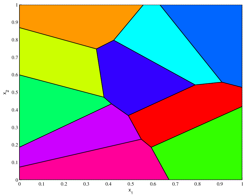
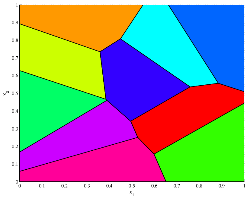
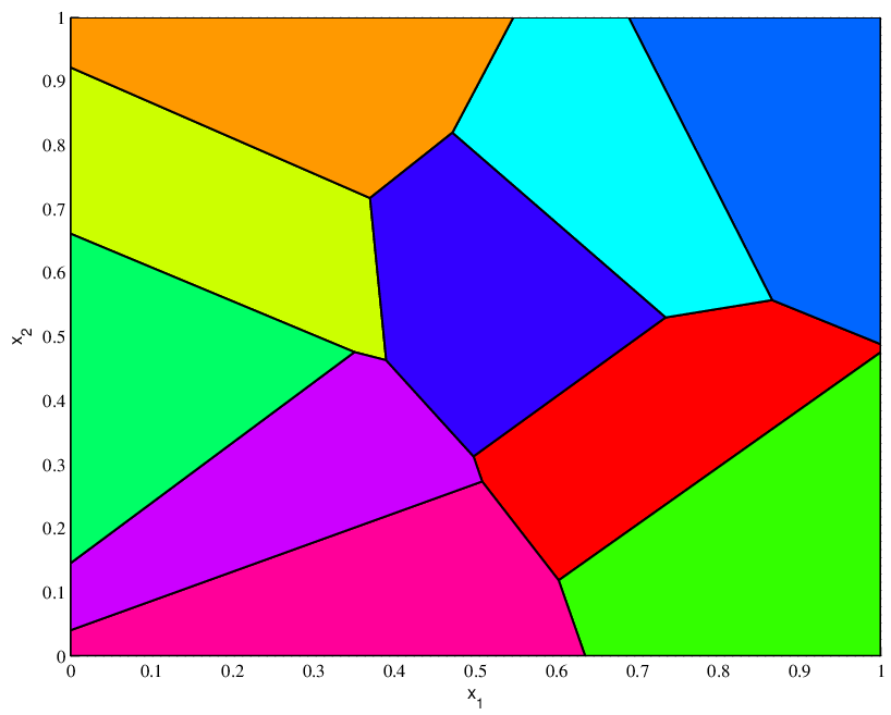
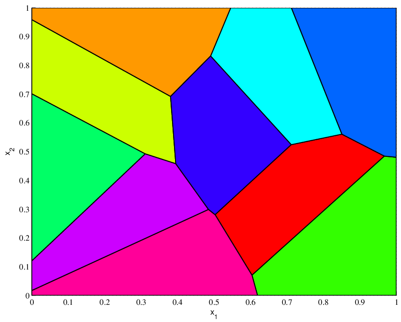
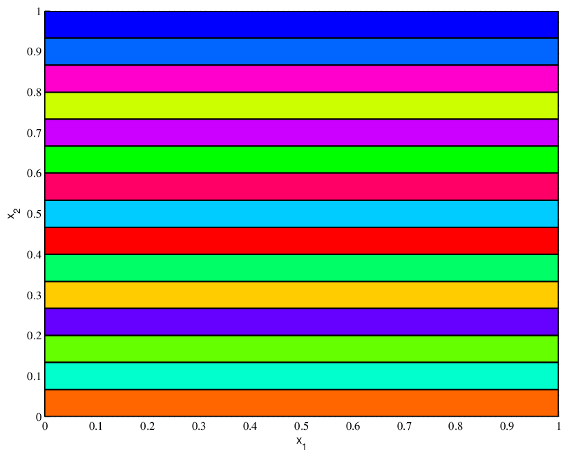
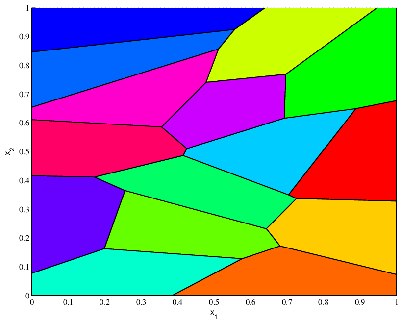
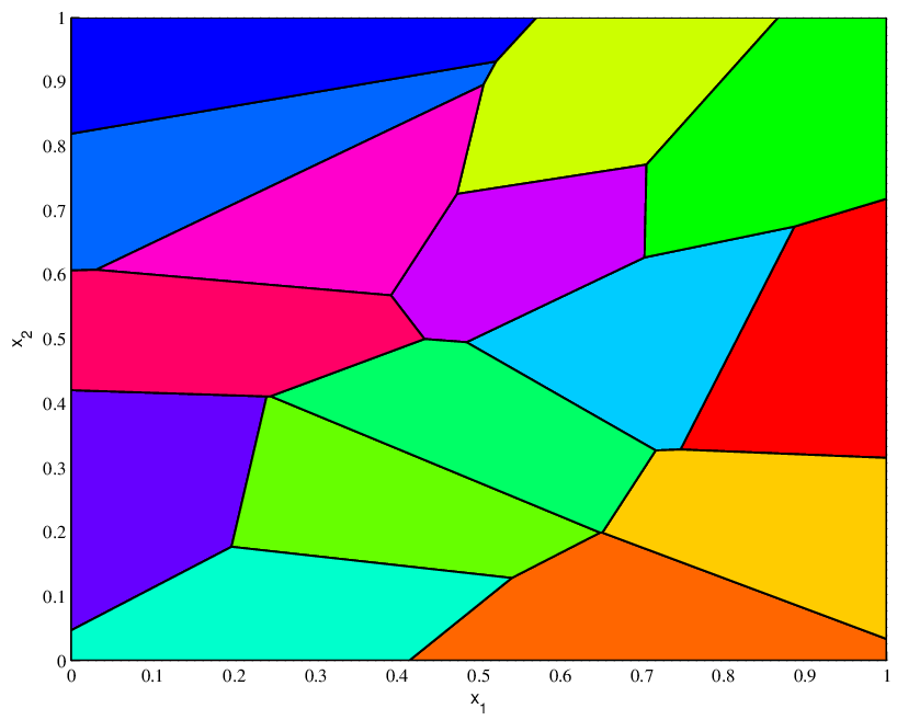
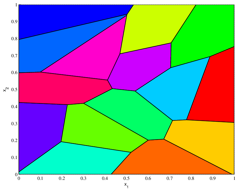
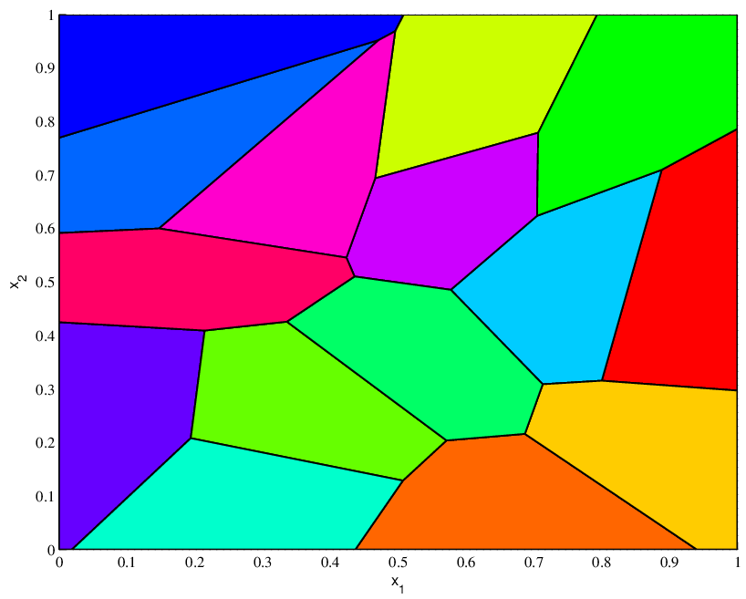
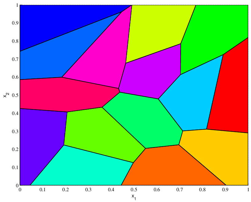
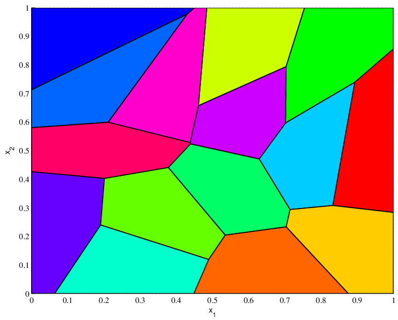
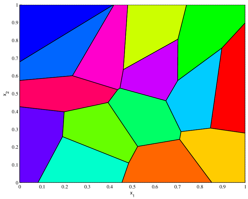
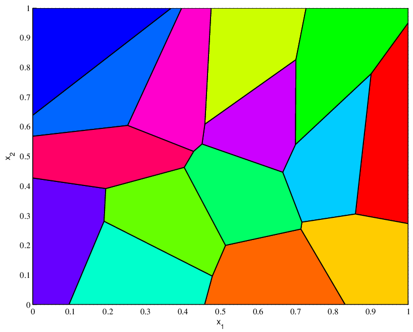
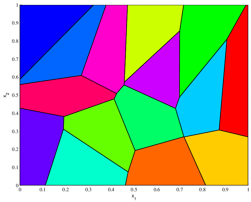
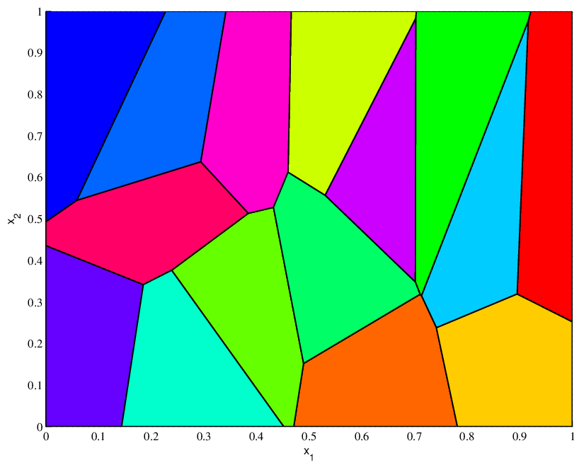
The construction of the cells at each step is achieved efficiently by an implementation in Matlab. In the setting described above where , , is the uniform distribution on , , our algorithm computes the cells as well as the prices of the cell for to . For which is the case where the transportation plan is the Knothe one, the computational task amounts to sorting the second component of the ’s. Appropriate discretization steps are then chosen for the transition to . At each step, the tesselation of into the polyhedral cells is computed based on the prices . Adjacency information on these cells is computed, as well as the length of the facet between two cells and the coordinates of its extreme points. This information allows one to formulate a discretized version of ODE (3.12) using an Euler discretization scheme.
For geometric computations we use the Multi-Parametric Toolbox library, available online at http://control.ee.ethz.ch/ mpt. In particular, polytope computes the tesselation of into the polyhedral cells . (A slighlty modified version of) mpt_buildAdjacency extracts adjacency information on this tesselation, from which the vertices and the lengths of the sides between two cells can be deduced. The library also incorporates convenient graphical routines.
Error analysis Some numerical examples are presented below, for which relative errors in cell areas (i.e. deviation from the optimality conditions) are given as well as a comparison between the tesselations obtained with our method and the true solution. Another way to test our method is as follows. Let us consider the set
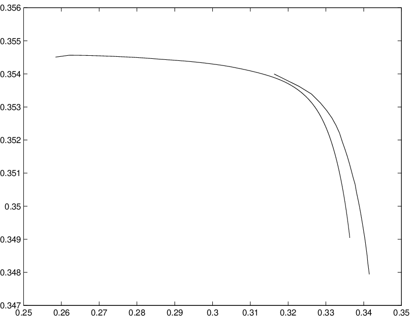
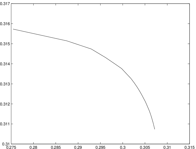
is a closed convex subset of and it is strictly convex in the sense that its boundary contains no line segment. Denoting by the solution of (3.1), it is easy to check that is an extreme point of and that is the equation of a supporting line of at and this supporting line intersects only at . If we consider the correlation curve it can be represented as the graph of a concave decreasing function whose slope (when it exists) at point is . In our numerical test, we will also present graphs comparing the true concave correlation curve to the one computed by our method.
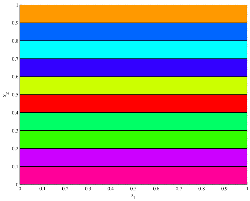
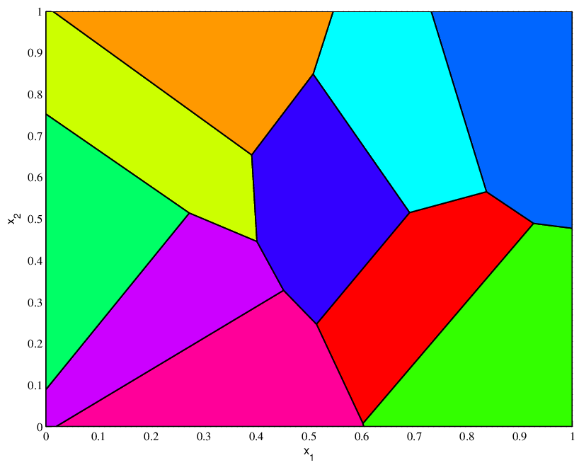
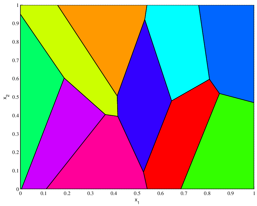
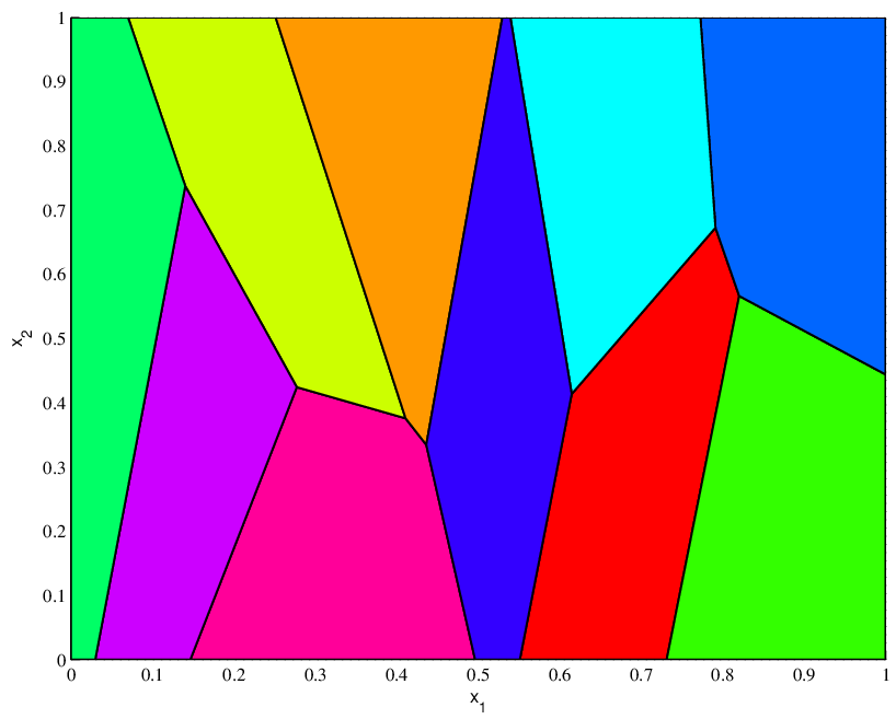
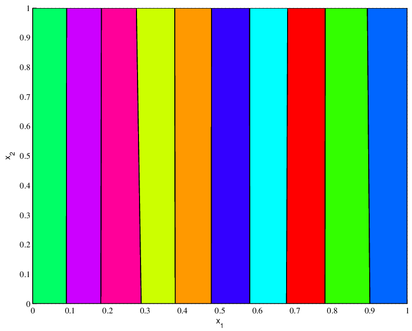
We give three instances of executions of our algorithm, with samples of respectively 5, 10, and 15 points. Taking weights with (rather than with ) we get the full evolution of the optimal transports from one Knothe’s transport (horizontal strips) to the other (vertical strips). Further examples as well as videos can be found at http://alfred.galichon.googlepages.com/anisotropic. It should also be pointed that our method does not approximate the solution of a single optimal transportation problem but a whole family of such problems (which actually explains relatively high running times).
Five sample points. We take as our sample set a sample of five points. We get the following errors:
|
|||||||||||||||||||||||
for which we draw in Figure 1 the partition obtained for using an exact method, as well as the true evolutions of the componentwise correlations of the ’s and the ’s from until .
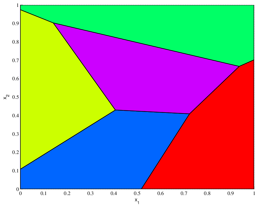
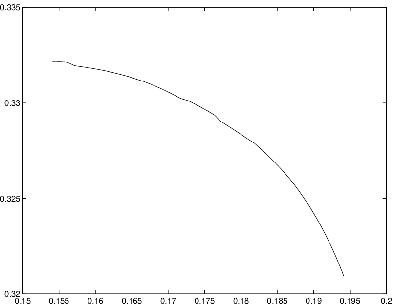
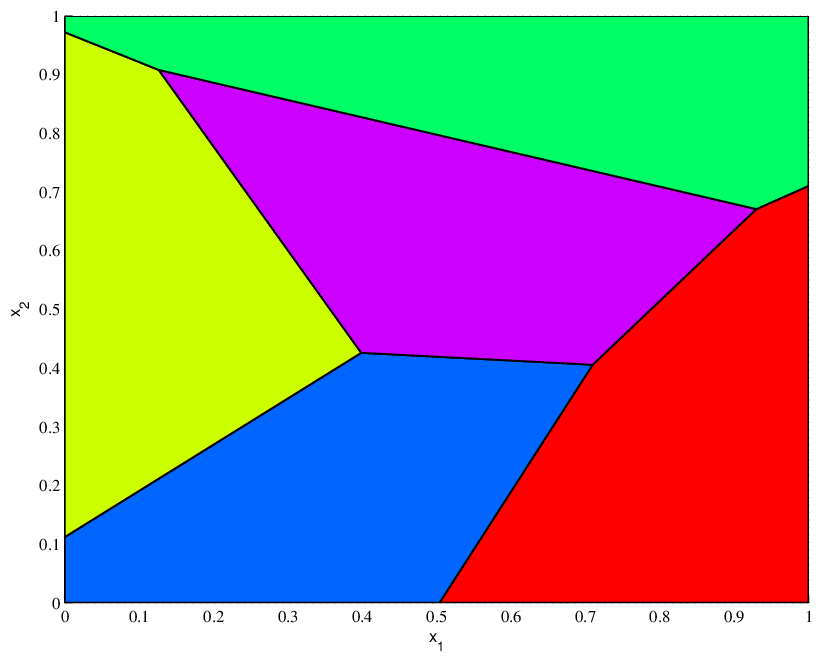
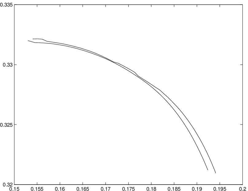
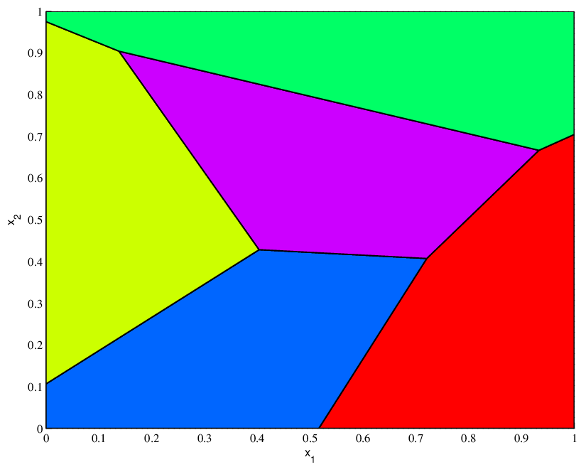
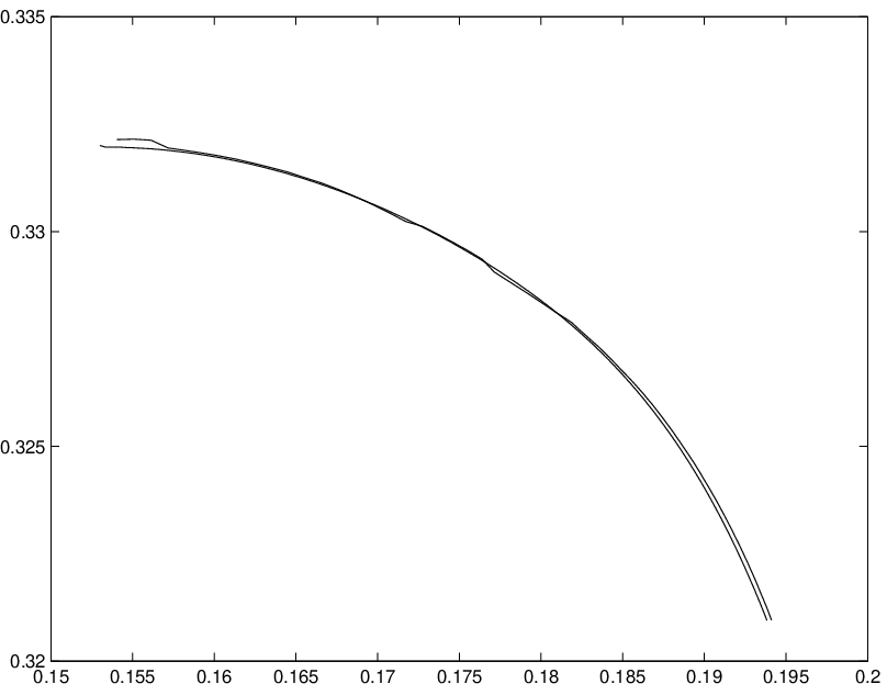
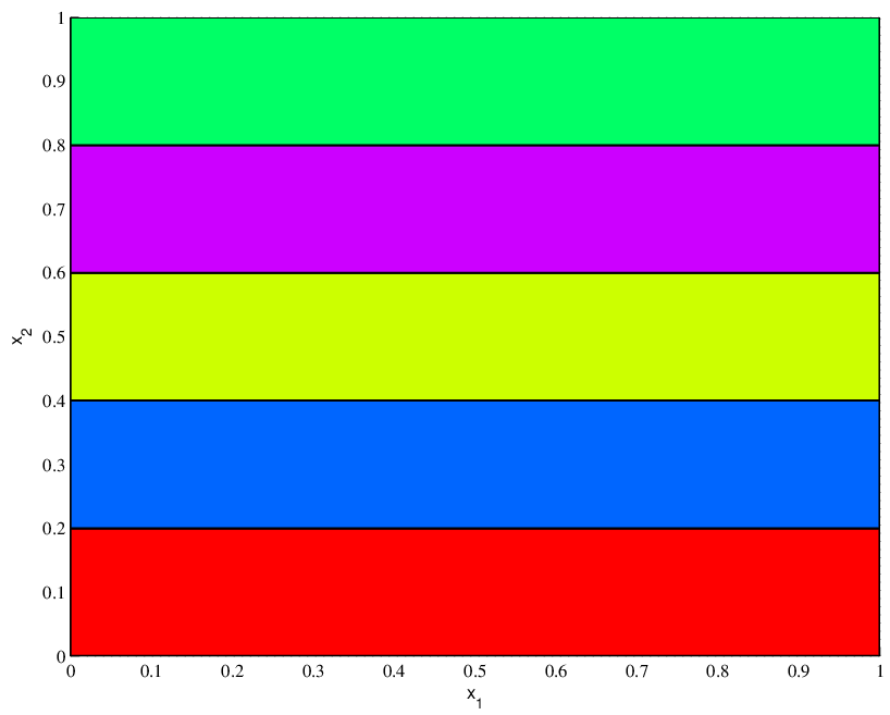
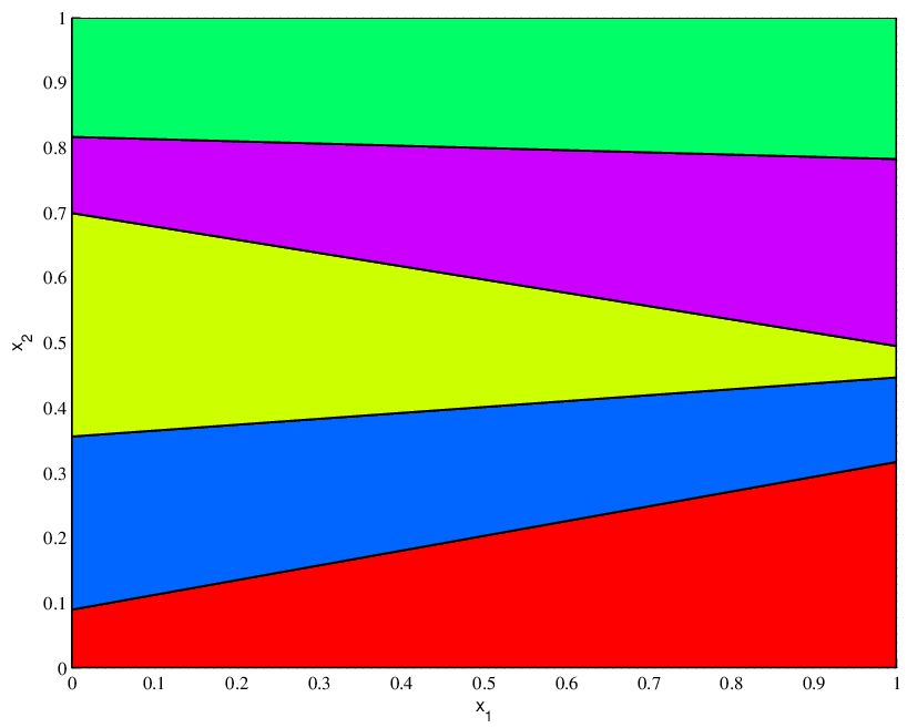
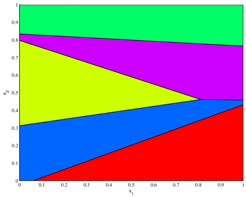
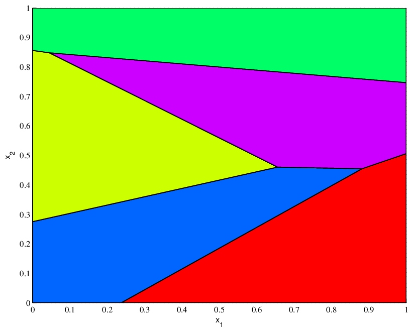
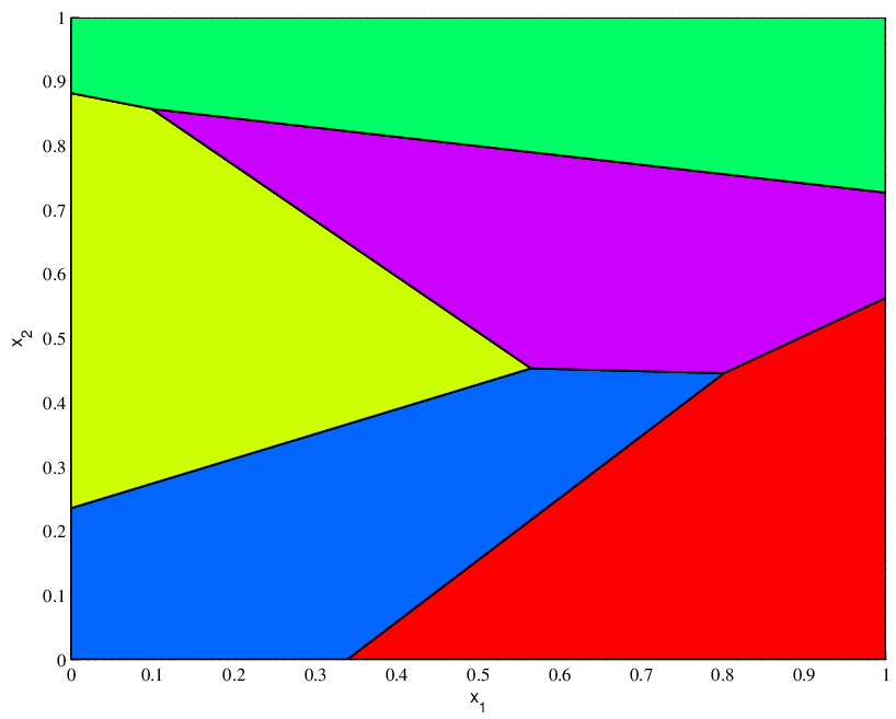
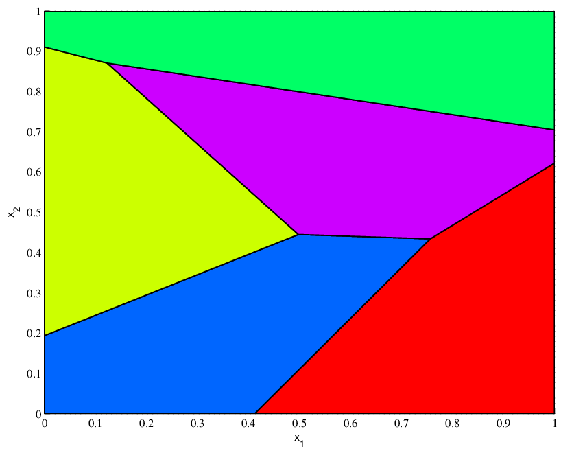
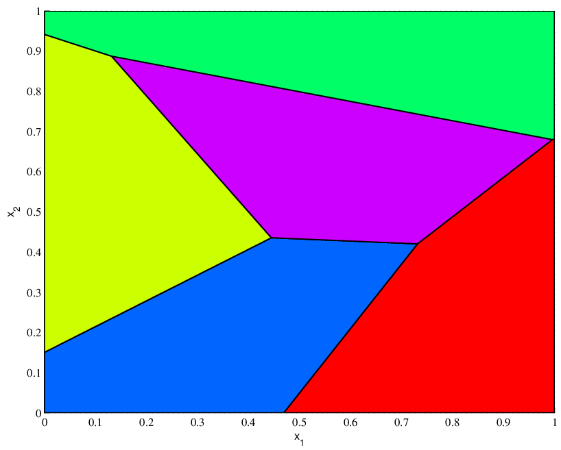
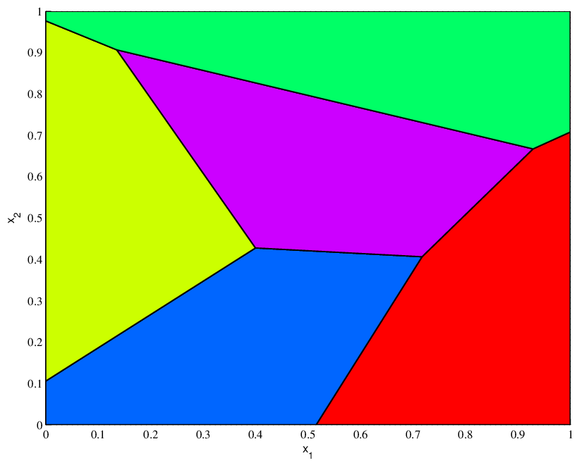
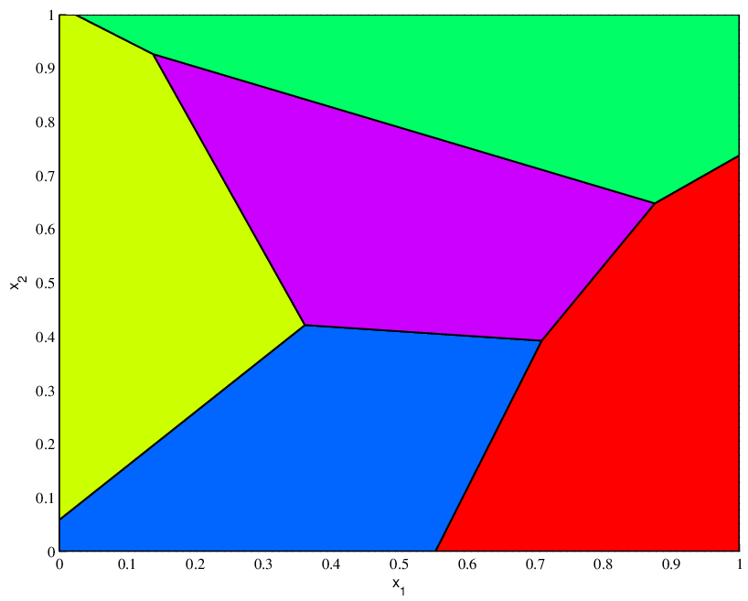
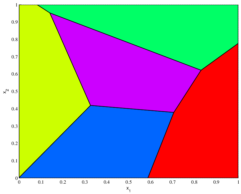
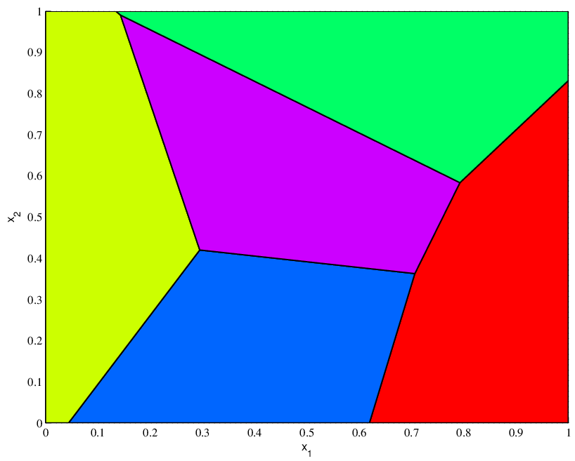
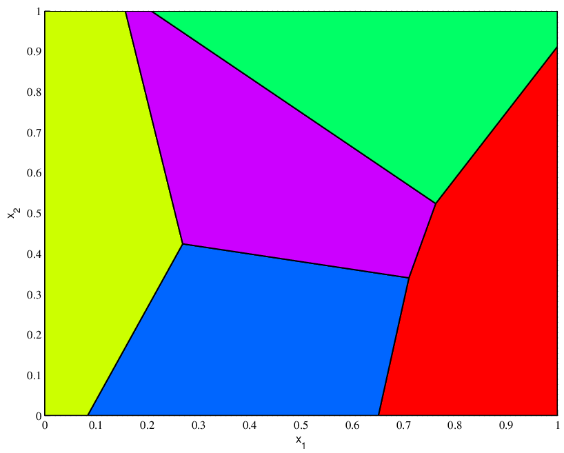
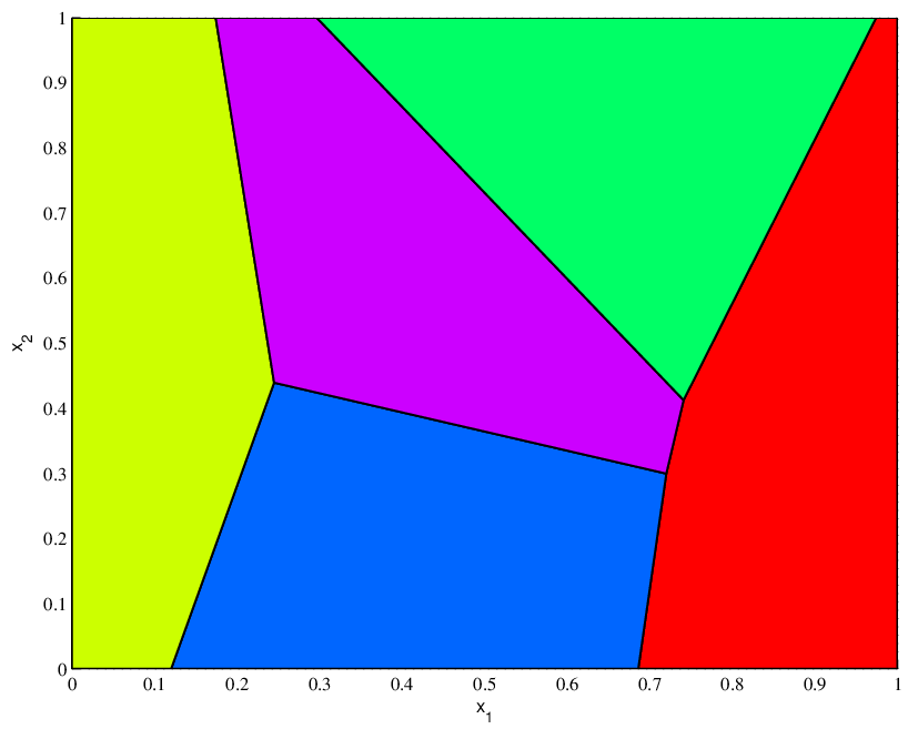
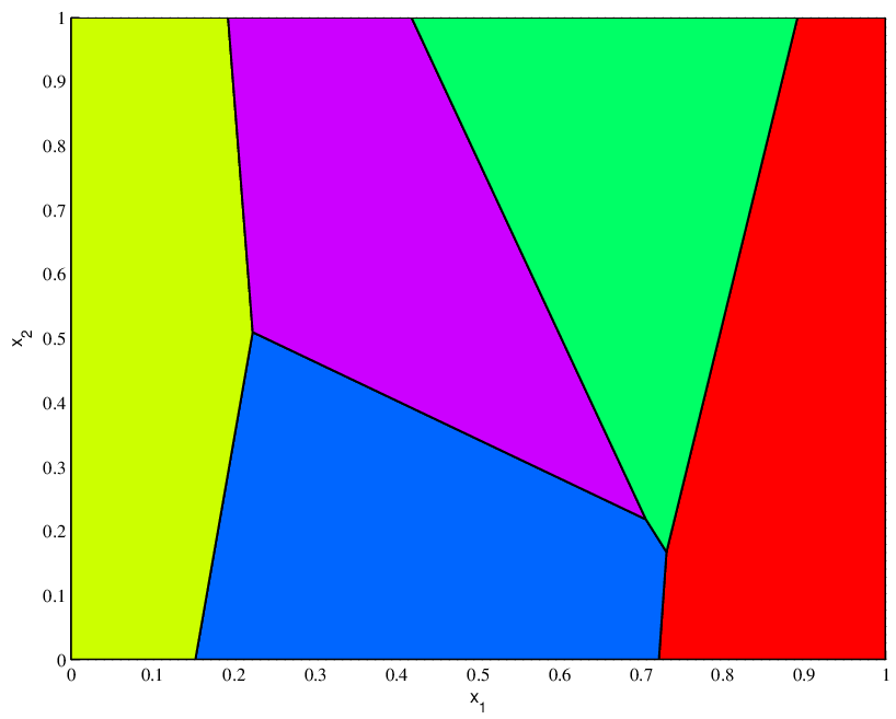
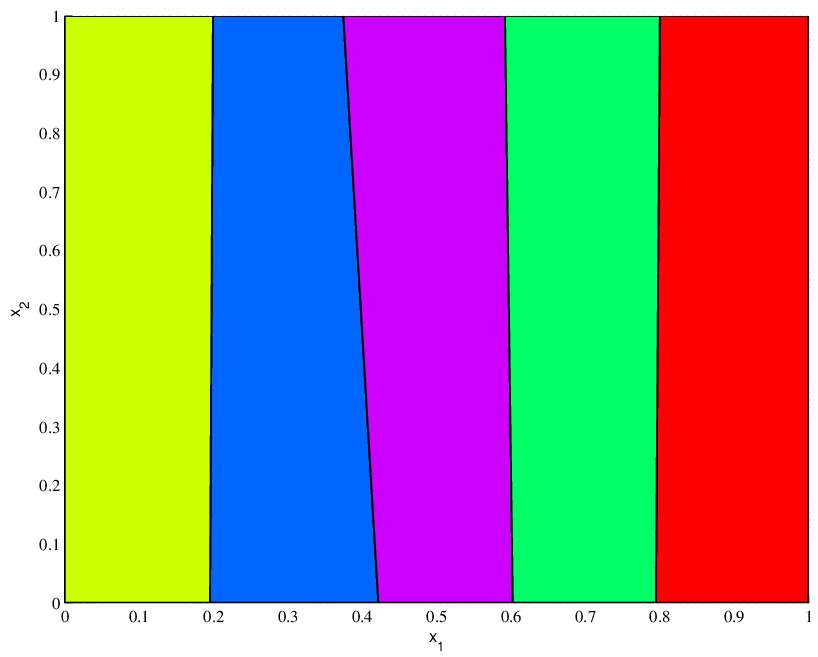
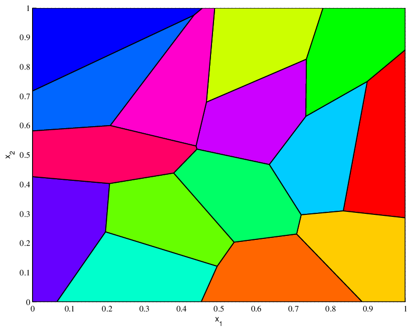
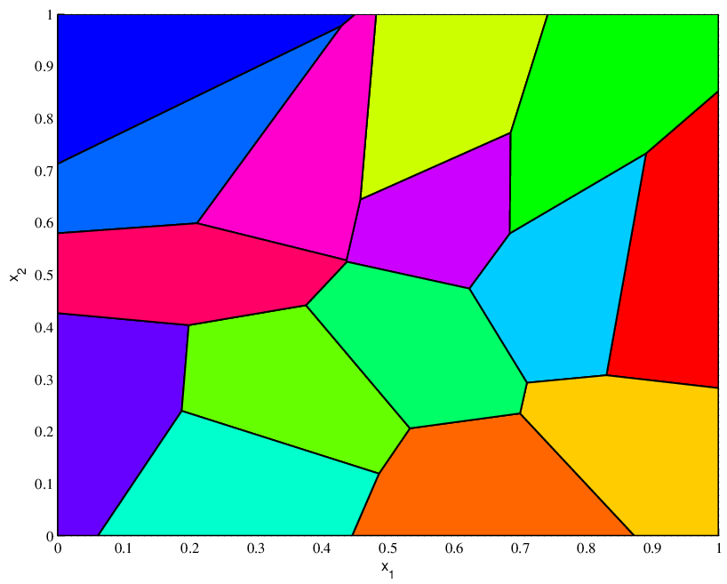
Running the continuation algorithm with 100 and 500 discretization steps we obtained partition sketched below, where the relative error on the cells area is inferior to 5%. The evolution of the componentwise correlations from until are also sketched and compared with their exact conterparts (the above curve). Running the algorithm with 500 discretization steps on a standard laptop took 349 seconds, and yields to the results below, where the maximal relative error on the cells area is 1%. The evolution of the componentwise correlations from until are also sketched and compared with their exact counterparts.
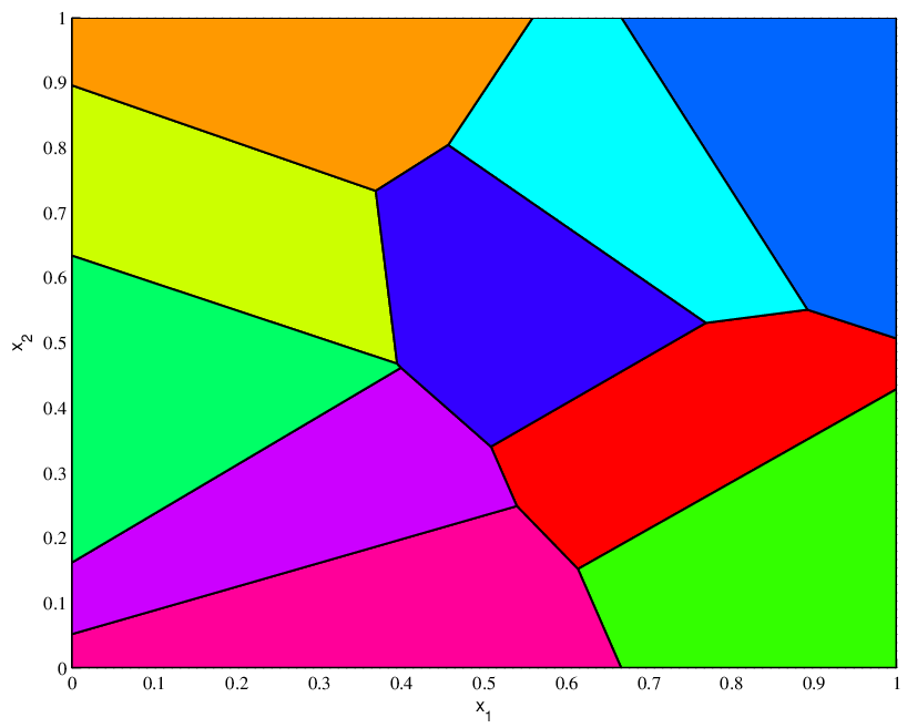
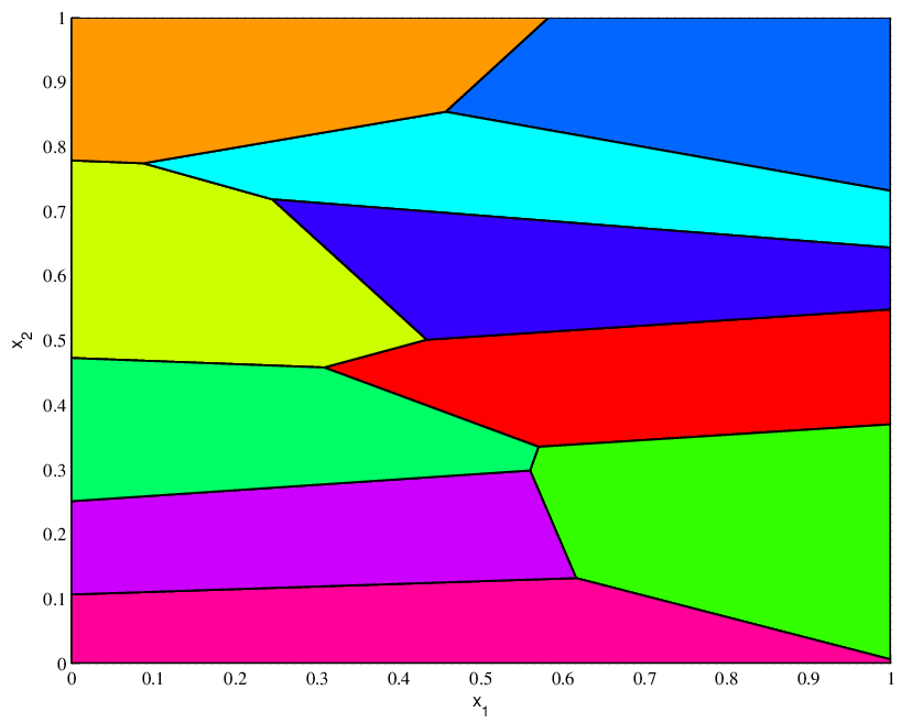
Ten sample points. Taking a sample of ten points, we obtain the following errors:
|
||||||||||||||||||||||||||||||||||||||||||||
We draw in Figure 3 the partition obtained for using an exact method, as well as the true evolutions of the componentwise correlations of the ’s and the ’s from until .
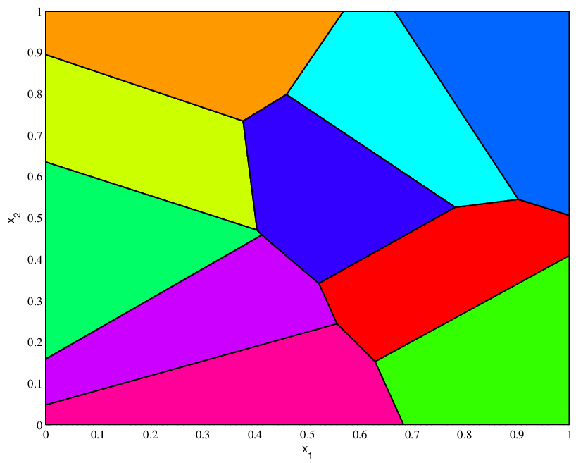
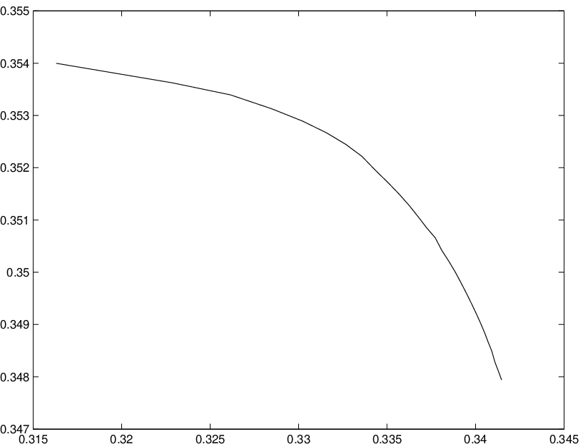
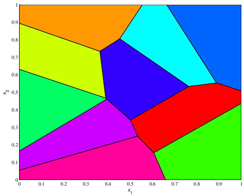

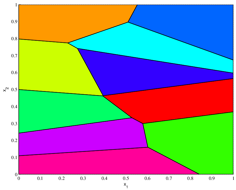
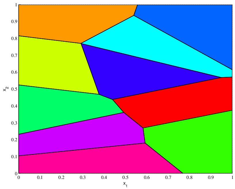
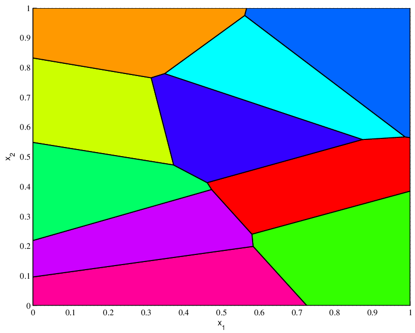
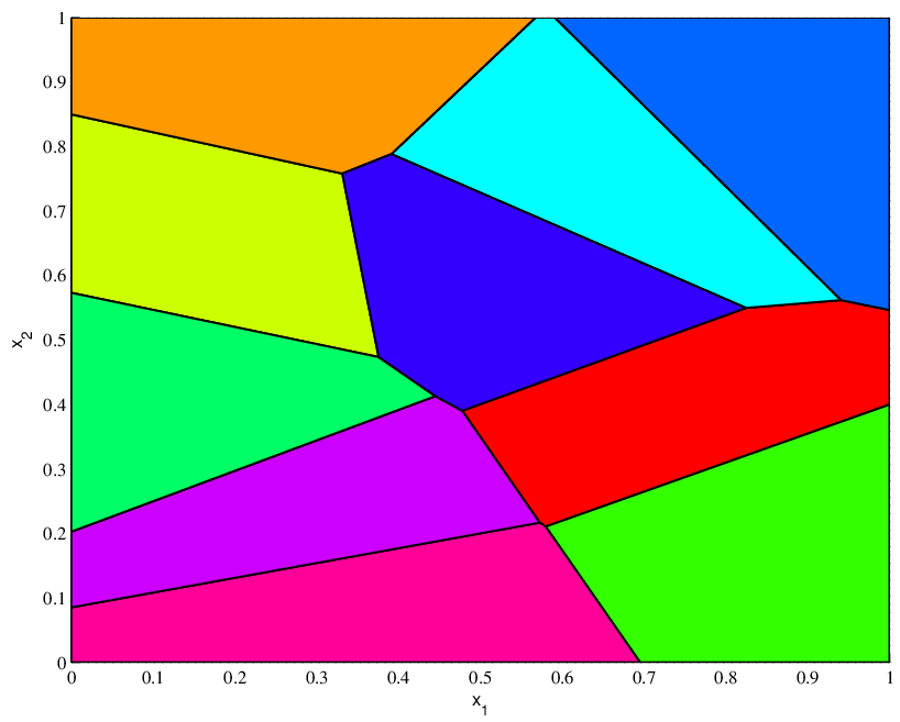

Fifteen sample points. With a sample of 15 points, we get the following errors:
|
|||||||||||||||||||||||||||||||||||||||||||||||||||||||||||||||||






Acknowledgements G.C. and F.S. gratefully acknowledge the support of the Agence Nationale de la Recherche via the research project OTARIE. A.G. gratefully acknowledge the support of Chaire EDF-Calyon “Finance et Développement Durable,” of Chaire AXA “Assurance et risques majeurs,” and of Chaire Société Générale “Risques Financiers”. The authors wish to warmly thank Yann Brenier and Alessio Figalli for stimulating discussions.
References
- [1] A. Braides, -convergence for beginners, Oxford University Press, Oxford, 2002.
- [2] Brenier, Y., Polar factorization and monotone rearrangement of vector-valued functions, Communications on Pure and Applied Mathematics 44, 375-417, 1991.
- [3] Crouzeix M., Mignot A.L, Analyse numérique des équations différentielles, Masson, Paris, 1984.
- [4] Knothe, H., Contributions to the theory of convex bodies, Michigan Mathematical Journal 4, pp. 39–52, 1957.
- [5] Rachev S.T., Rüschendorf L., Mass Transportation Problems. Vol. I: Theory; Vol. II : Applications, Springer-Verlag 1998.
- [6] Rosenblatt, M., Remarks on a multivariate transformation, Annals of Mathematical Statistics 23, pp. 470–472, 1952.
- [7] Villani, C., Topics in Optimal Transportation, Providence: American Mathematical Society, 2003.
- [8] Villani, C., Optimal transport: Old and New, lecture notes, Ecole d’été de probabilités de Saint-Flour, to appear, New York: Springer, 2008.