Localization of maximal entropy random walk

Since the seminal papers by Einstein [1] and Smoluchowski [2] which formulated the theory of Brownian motion and diffusive processes, a discrete-time realization of these processes, random walk (RW), has continuously attracted attention. Random walk has been discussed in thousands of scientific papers and textbooks in statistical physics, economics, biophysics, engineering, particle physics, etc., and is still an active research area (see e.g. [3]). Mathematically speaking, random walk is a Markov chain which describes the trajectory of a particle (random walker) taking successive random steps. In the simplest variant, random walk on a lattice, at each time step the particle chooses at random one of the adjacent nodes and jumps to it. In the continuum limit, the probability density of finding the particle at a given position obeys the diffusion equation. When the lattice is regular, it is easy to show that all trajectories (sequences of nodes visited by the particle) of a given length between two given points of the lattice are equiprobable, and thus have maximal entropy. Therefore, drawing an analogy with the path-integral formalism [4], trajectories are weighted only by their length, which plays the role of the action in the absence of potential energy.

In this Letter we ask what changes if one takes the above statement as a definition of RW. In other words, we define random walk not by local hopping rules but by the requirement that RW trajectories maximize entropy. We shall see that, if the lattice is not regular, this new definition leads to a dramatic change in the behavior of RW. Let us summarize our main results. First, we define the maximal entropy random walk (MERW) and show that it indeed maximizes the entropy of trajectories, in contrast to generic random walk (GRW), which has smaller entropy. Second, we discuss a surprising effect of localization of MERW trajectories in the presence of weak disorder. This is a purely classical example of the Lifshitz phenomenon [5]. Some kind of localization has been observed before in RW on networks with a broad distribution of nodes degrees [6], but for MERW the effect is completely different in nature, since it can be triggered by any small amount of inhomogeneity.

To begin, let us consider quite generally a particle hopping randomly from node to node on a given finite, connected graph. The graph is defined by a symmetric adjacency matrix $A$, with elements $A_{ij}=1$ if $i$ and $j$ are neighboring nodes and $A_{ij}=0$ otherwise. The hopping is a local Markov process: the particle which arrives at some moment to node $i$ will hop to a neighboring node $j$ with probability $P_{ij}$, independently of the past history. The elements of the transition matrix are $P_{ij}=0$ if $A_{ij}=0$, that is if nodes $i,j$ are not linked, and for each $i$ one has $\sum_{j}P_{ij}=1$.

The main quantity of interest is the probability, $\pi_{i}(t)$, of finding the particle at node $i$ at time $t$. One can calculate it recursively, applying the Markov property:

$$\pi_{i}(t+1)=\sum_{j}\pi_{j}(t)P_{ji}.$$

(1)

Using spectral properties of the matrix $P_{ij}$, one can show that $\pi_{i}(t)$ reaches for $t\rightarrow\infty$ a unique stationary state $\pi_{i}^{*}$ obeying the following eigenequation:

$$\pi_{i}^{*}=\sum_{j}\pi_{j}^{*}P_{ji}.$$

(2)

For GRW, $P_{ij}=A_{ij}/k_{i}$, where $k_{i}=\sum_{j}A_{ij}$ is the number of neighbors of node $i$ (node degree). This means that the particle hops to an adjacent node with the same probability for all neighbors. The stationary distribution of GRW reads

$$\pi_{i}^{*}=\frac{k_{i}}{\sum_{j}k_{j}}.$$

(3)

Another quantity of interest, especially important from the point of view of RW entropy, is the probability $P(\gamma^{(t)}_{i_{0}i_{t}})$ of generating a trajectory $\gamma_{i_{0}i_{t}}^{(t)}$ of length $t$, passing through nodes $(i_{0},i_{1},\ldots,i_{t-1},i_{t})$:

$$P(\gamma^{(t)}_{i_{0}i_{t}})=P_{i_{0}i_{1}}P_{i_{1}i_{2}}\ldots P_{i_{t-1}i_{t}}.$$

(4)

In general $P(\gamma^{(t)}_{i_{0}i_{t}})$ depends on all nodes on the trajectory. For GRW we have

$$P(\gamma^{(t)}_{i_{0}i_{t}})=\frac{1}{k_{i_{0}}k_{i_{1}}\ldots k_{i_{t-1}}},$$

(5)

and we see that the trajectories are not equiprobable. An exception is GRW on a $k$-regular graph, whose nodes have identical degrees, as for instance on a regular lattice. In general, however, trajectories produced by GRW are not maximally random. As we will see below, there exists, though, a choice of $P_{ij}$ such that all trajectories of given length $t$ and given endpoints are equiprobable. This choice corresponds to MERW.

Let us now present the explicit construction of MERW. Let $\psi_{i}$ be the normalized eigenvector, $\sum_{i}\psi_{i}^{2}=1$, corresponding to the maximal eigenvalue $\lambda$ of the adjacency matrix $A_{ij}$:

$$\sum_{j}A_{ij}\psi_{j}=\lambda\psi_{i}.$$

(6)

The eigenvalue $\lambda$ is clearly in the range $k_{\rm min}\leq\lambda\leq k_{\rm max}$, where $k_{\rm min}$ and $k_{\rm max}$ are the maximal and minimal node degrees of the graph, respectively. The Frobenius-Perron theorem tells us that the eigenvector has all elements of the same sign, so that one can choose $\psi_{i}>0$. Let us use this eigenvector to define the following transition matrix:

$$P_{ij}=\frac{A_{ij}}{\lambda}\frac{\psi_{j}}{\psi_{i}}.$$

(7)

By construction, the entries $P_{ij}$ are positive if $i$ and $j$ are neighboring nodes. They are also properly normalized: $\sum_{j}P_{ij}=1$. A similar construction has been recently proposed in the context of optimal information coding [7]. The weight (4) is now independent of intermediate nodes:

$$P(\gamma^{(t)}_{i_{0}i_{t}})=\frac{1}{\lambda^{t}}\frac{\psi_{i_{t}}}{\psi_{i_{0}}},$$

(8)

and thus all trajectories having length $t$ and given endpoints $i_{0}$ and $i_{t}$ are equiprobable. For a closed trajectory, the probability (8) depends only on its length $t$. The stationary distribution of MERW is

$$\pi_{i}^{*}=\psi_{i}^{2},$$

(9)

which is easy to check by combining Eqs. (7) and (2). It is a normalized probability: $\sum_{i}\pi_{i}^{*}=1$, and the detailed balance condition is fulfilled: $\pi_{i}^{*}P_{ij}=\pi_{j}^{*}P_{ji}$.

We intuitively see that random trajectories generated by the transition probabilities $(\ref{merw})$ are more random than those generated by GRW since now the probability of a given random path (8) is independent of intermediate nodes. This statement can be quantified by comparing the entropy rates of the corresponding Markov processes. Let $P(i_{0},i_{1},\ldots,i_{t})$ be the probability of a sequence $(i_{0},i_{1},\ldots,i_{t})$ in the set of all sequences of length $t$ generated by the Markov chain. The Shannon entropy in this set of sequences is:

$$S_{t}=-\sum_{i_{0},i_{1}\dots i_{t}}P(i_{0},\ldots,i_{t})\ln P(i_{0},\ldots,i_{t}).$$

(10)

One can show [8], using the Markov property of the chain: $P(i_{0},i_{1},\ldots,i_{t})=\pi_{i_{0}}P_{i_{0}i_{1}}\ldots P_{i_{t-1}i_{t}}$, that for large $t$ the entropy $S_{t}$ increases at a fixed rate

$$s\equiv\lim_{t\rightarrow\infty}\frac{S_{t}}{t}=-\sum_{i}\pi^{*}_{i}\sum_{j}P_{ij}\ln P_{ij},$$

(11)

which is independent of the initial distribution $\pi_{i}$. For GRW, with $P_{ij}=A_{ij}/k_{i}$ and $\pi^{*}_{i}$ from Eq. (3), we obtain the entropy production rate

$$s_{\rm GRW}=\frac{\sum_{i}k_{i}\ln k_{i}}{\sum_{i}k_{i}},$$

(12)

while MERW, with transition rates (7) and the stationary distribution (9), yields $s_{\rm MERW}=\ln\lambda.$ We now show that $s_{\rm MERW}$ is indeed the maximal entropy rate which can be obtained for any stochastic process generating trajectories on the graph. The number of trajectories of length $t$ on the graph is $N_{t}=\sum_{i,j}(A^{t})_{ij}$, where $A^{t}$ is the $t$-th power of the adjacency matrix. In the $t\rightarrow\infty$ limit we obtain the following asymptotic value:

$$s_{\rm MAX}=\lim_{t\rightarrow\infty}\frac{\ln N_{t}}{t}=\ln\lambda,$$

(13)

which sets the upper limit for the entropy rate of such processes. We see that $s_{\rm MERW}=s_{\rm MAX}$, so that MERW indeed maximizes the entropy and the corresponding trajectories are maximally random. As a byproduct we obtain a lower bound for the largest eigenvalue of the adjacency matrix:

$$\ln\lambda\geq\frac{\sum_{i}k_{i}\ln k_{i}}{\sum_{i}k_{i}},$$

(14)

which we have not found in the literature. For a $k$-regular graph, $s_{\rm GRW}=s_{\rm MERW}=\ln k$. Similarly, for a bipartite graph which has nodes of degree $k$ in one partition and of degree $k^{\prime}$ in the other one, $s_{\rm GRW}=s_{\rm MERW}=\frac{1}{2}\ln(kk^{\prime})$.

As already mentioned, GRW and MERW are identical on a $k$-regular graph. For example, GRW on a square lattice is maximally random. The question arises how much the two types of random walk differ on a graph or lattice with some irregularities. For definiteness, imagine that we remove at random a small fraction $q\ll 1$ of non-adjacent links from an $L\times L$ square lattice with periodic boundary conditions. In this way we obtain a lattice with a weak disorder (dilution), where most of the nodes are of degree $k=4$ and some of degree $k=3$. The stationary distribution $\pi_{i}^{*}$ for GRW is given by Eq. (3), so that the probability of finding the particle after long time at a defective node is equal to 3/4 of the probability at an intact one. The situation looks completely different for MERW, as shown in Fig. 1, presenting density plots of $\pi_{i}^{*}$ for different densities of defects, obtained by diagonalizing $A$ numerically and using Eq. (9). For a very low density $q$ of defects, the probability $\pi_{i}^{*}$ is smaller in the neighborhood of defects, like in the GRW case. However, if the number of defects increases, the stationary distribution $\pi_{i}^{*}$ becomes localized in a nearly circular region. We will indeed argue, using the Lifshitz argument [5], that this localization phenomenon is observed for any finite fraction of defects provided the linear size $L$ of the system is large enough, and that the radius of the localization region grows as $(\ln L)^{1/2}$.

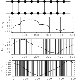
Let us start with a 1d example, in order to build up some intuition. One cannot of course use a one-dimensional chain, since removing a single link would disconnect it. Instead, we shall consider, as a model example, a ladder graph with periodic boundary conditions, with a fraction $q$ of randomly removed rungs, as shown in Fig. 2. In order to define the transition probabilities (7) we have to solve the eigenproblem of the adjacency matrix $A$. Let $L$ be length of the ladder. Taking into account the symmetry between both legs, we have:

$$\psi_{i+1}+\psi_{i-1}+r_{i}\psi_{i}=\lambda\psi_{i},$$

(15)

where the index $i$ runs over the $L$ nodes in the lower leg of the ladder, say, and $r_{i}=1$ if there is a rung at the position $i$, and $r_{i}=0$ otherwise. Introducing the discrete Laplacian $\Delta_{ij}=\delta_{i,j+1}+\delta_{i,j-1}-2\delta_{ij}$, Eq. (15) can be recast as

$$-(\Delta\psi)_{i}+v_{i}\psi_{i}=E\psi_{i},$$

(16)

where $E=3-\lambda$, whereas $v_{i}=1-r_{i}$ form a random binary sequence with a frequency of unities or defects ($v_{i}=1$) equal to $q$ and a frequency of zeros ($v_{i}=0$) equal to $p=1-q$. Each sequence of sites without defects ($v_{i}=0$) is said to form a well. Eq. (16) is formally identical to the eigenvalue equation of the following trapping problem. A particle performs a random walk in continuous time on the 1d lattice. Defects act as static traps: whenever the particle sits at site $i$, it is annihilated at rate $v_{i}$ per unit time. Trapping problems of this kind have been studied extensively [9]. The asymptotic long-time fall-off of the survival probability is known to be related to the so-called Lifshitz tail in the density of states of Eq. (16) as $E\to 0$. In the present context, the Lifshitz argument [5] predicts that the ground state of Eq. (16) is well approximated by that of the longest well, i.e., $-(\Delta\psi)_{i}=E_{0}\psi_{i}$ ($i=1,\dots,w$), with Dirichlet boundary conditions $\psi_{0}=\psi_{w+1}=0$, where $w$ is the length of that well. We obtain $\psi_{i}\sim\sin(i\pi/(w+1))$ and $E_{0}=2(1-\cos\pi/(w+1))\approx\pi^{2}/w^{2}$. In the 1d situation [10], this argument is known to essentially give an exact description of the ground-state.

In the case of MERW, we therefore predict that the whole stationary probability is asymptotically localized on the longest well, i.e., the longest sequence without defects. The Lifshitz picture is indeed a good approximation, as one can see in Fig. 2, showing the density $\pi_{i}^{*}$, obtained by numerical diagonalization of $A$. The length $w$ of the longest well can be estimated as follows. The mean number of unities in the sequence grows as $Lq$. The mean number of those followed by one zero is $Lqp$, by two zeros is $Lqp^{2}$, and so on, so that there are $Lqp^{n}$ wells of length $n$, i.e., consisting of $n$ zeros. The length of the longest well is then given by $Lqp^{w}\sim 1$. Hence it grows logarithmically with the system size, $w\approx\ln L/|\ln p|$, so that $E_{0}\approx(\pi|\ln p|/\ln L)^{2}$. In Fig. 3 we show that the ground-state energy $E_{0}$ obtained by numerically solving Eq. (16), averaged over binary disorder for $q=0.1$, agrees with the above estimate for $L$ large enough.

The Lifshitz argument can be generalized to higher-dimensional lattices [11]. The ground state of the discretized Schrödinger equation (16) is localized in the largest Lifshitz sphere, defined as the largest nearly spherical region of the lattice which is free of defects. Taking again for definiteness the example of the square lattice, the radius $R_{\rm max}$ of the largest Lifshitz disk and the corresponding ground-state energy $E_{0}$ can be evaluated as follows. The number of circular regions of radius $R$ with no defects is of order $L^{2}p^{2\pi R^{2}}$, as there are two links per node, so that $R_{\rm max}\approx(\ln L/(\pi|\ln p|))^{1/2}$. In the continuum limit, the ground state in the disk of radius $R$ is given by $\psi(r)\sim J_{0}(jr/R)$, where $r$ is the distance from the center and $j\approx 2.405$ is the first zero of the Bessel function $J_{0}$. We thus obtain $E_{0}\approx(j/R_{\rm max})^{2}\approx\pi j^{2}|\ln p|/\ln L$. In higher dimension, skipping constants, the above estimates read $R_{\rm max}\sim(\ln L/|\ln p|)^{1/d}$ and $E_{0}\sim(|\ln p|/\ln L)^{2/d}$. Hence the stationary probability of MERW on a $d$-dimensional lattice in the presence of any amount of disorder is localized in the largest Lifshitz sphere, whose volume grows asymptotically as $\ln L$.

The above picture allows one to address dynamical issues. Imagine a random walker starting at a random site. In the course of evolution it will find a moderately large region free of defects, a sort of local Lifshitz sphere, and spend some time there before it will make an excursion to another, larger local Lifshitz sphere, etc. The process will look very much like going through consecutive metastable states before finally reaching the true ground state. Metastable states are formed not because of energy barriers, but because of entropy barriers [12], as MERW favors regions where it can maximize entropy. It is therefore tempting to consider MERW as a model of evolution in a flat fitness landscape.

Let us close up with a comment on the connection with the path-integral formalism [4]. In the simplest case of a free particle propagating in curved space-time from $a$ to $b$, the quantum amplitude is

$$K_{ab}=\sum_{t}\sum_{\gamma^{(t)}_{ab}}{\rm e}^{-S_{\rm E}},$$

(17)

where the Euclidean action $S_{\rm E}$ is proportional to time $t$. One would naively expect that all the trajectories $\gamma_{ab}^{(t)}$ should be equiprobable. We know, however, that the propagator $K_{ab}$ of a massless scalar field is equal to the inverse of the graph Laplacian $\Delta_{ab}=\sqrt{k_{a}k_{b}}\delta_{ab}-A_{ab}$ which can be expressed as a sum over GRW and not MERW trajectories. It would be interesting to check to what extent the continuum theory would differ if one constructed quantum amplitudes using MERW instead of GRW trajectories.

In conclusion, we have shown that GRW maximizes local entropy and MERW maximizes global entropy of random trajectories. This little change in the definition of random walk leads to a dramatic change in the statistical properties of the system in the presence of a weak disorder.

We would like to thank P. Bialas and F. David for discussions. This work was supported in part by the Marie Curie Actions Transfer of Knowledge project “COCOS” – grant No. MTKD-CT-2004-517186, the EC-RTN Network “ENRAGE” – grant No. MRTN-CT-2004-005616 and the Polish Ministry of Sciences and Information Technologies – grant 1P03B-04029 (2005-2008).

References

- [1] A. Einstein, Ann. Physik 17, 547 (1905); 19, 371 (1906).
- [2] M. Smoluchowski, Ann. Physik 21, 756 (1906).
- [3] C. Anteneodo and W.A.M. Morgado, Phys. Rev. Lett. 99, 180602 (2007); S.N. Majumdar and R. M. Ziff, Phys. Rev. Lett. 101, 050601 (2008).
- [4] R.P. Feynman and A.R. Hibbs, Quantum Mechanics and Path Integrals, Mc Graw-Hill, New York (1965).
- [5] I.M. Lifshitz, Adv. Phys. 13, 483 (1964); Sov. Phys. – Uspekhi 7, 549 (1965).
- [6] J. D. Noh and H. Rieger, Phys. Rev. Lett. 92, 118701 (2004).
- [7] J. Duda, arXiv:0710.3861.
- [8] B. McMillan, Ann. Math. Statist. 24, 196 (1953); C. Shannon, Bell System Tech. J. 27, 379 (1974); 27, 623 (1974).
- [9] B.Y. Balagurov and V.G. Vaks, Sov. Phys. – J.E.T.P. 38, 968 (1974); M.D. Donsker and S.R.S. Varadhan, Commun. Pure Appl. Math. 28, 525 (1975); 32, 721 (1979); P. Grassberger and I. Procaccia, J. Chem. Phys. 77, 6281 (1982); J.W. Haus and K.W. Kehr, Phys. Rep. 150, 263 (1987).
- [10] Th.M. Nieuwenhuizen, Physica A 167, 43 (1990); J.M. Luck, Systèmes Désordonnés Unidimensionnels, Collection Aléa-Saclay (1992), and the references therein.
- [11] L. Pastur, Russ. Math. Surv. 28, 1 (1973); R. Friedberg and J.M. Luttinger, Phys. Rev. B 12, 4460 (1975); S. Nakao, Jpn. J. Math. 3, 111 (1977); W. Kirsch and F. Martinelli, Commun. Math. Phys. 89, 27 (1983).
- [12] F. Ritort, Phys. Rev. Lett. 75, 1190 (1995); F. Ritort and P. Sollich, Advances in Physics 52, 219 (2003).